Missile Autopilot Design ViaFunctional Inversion andTime-Scaled Transformation

JAE-HYUK OH

IN-JOONG HASeoul National University

This paper presents a new approach to acceleration control of

STT (Skid-To-Turn) missiles. In the design and stability analysis

of our autopilot, we assume perfect roll-stabilization but consider

fully all other nonlinearities of the missile dynamics including the

coupling effect due to bank angle. Our autopilot controller consists

of a partial-linearizing controller and a dynamic compensator.

The partial-linearizing controller along with a time-scaled

transformation can convert the nonlinear missile dynamics to

the so-called normalized system which is completely independent

of Mach number and almost independent of air density. The

dynamic compensator is designed based on this normalized

system. This normalized system greatly simplifies the design

process of an autopilot controller regardless of flight conditions.

Our autopilot controller can provide fast and exact set-point

tracking performance but without the slow-varying conditions

on angle of attack and side-slip angle required often in the prior

works.

Manuscript received July 14, 1994; revised July 14, 1995.

IEEE Log No. T-AES/33/1/01075.

Authors’ address: Dept. of Control and Instrumentation Engineering,Automatic Control Research Center, Seoul National University, San56-1 Shinrim-Dong, Kwanak-Ku, Seoul 151-742, Korea.

0018-9251/97/$10.00 c° 1997 IEEE

I. NOMENCLATURE

(X,Y,Z) Missile body coordinate systemi,j,k Unit vectors along the X-, Y-, Z-axes,

respectivelyU,V,W X-, Y-, Z-components, respectively, of

the linear velocity vector of themissile

p,q,r X-, Y-, Z-components, respectively, ofthe angular velocity vector of themissile

Iy,Iz Moments of inertia about Y-, Z-axes,respectively

Ixy,Iyz ,Izx Products of inertiaVS Velocity of soundVM Total velocity of the missile

(¢=pjUj2 + jVj2 + jWj2 )

M Mach number (¢=VM=VS)

° Total angle

(¢=tan¡1(

pjVj2 + jWj2=VM))

®,¯,Á Angle of attack, side-slip angle, bank

angle (®¢=tan¡1(W=U),

¯¢=tan¡1(V=U), Á

¢=tan¡1(W=V))

m Missile mass½ Air densityQ Dynamic pressure (

¢= ½jVM j2=2)

S Aerodynamic reference areaD Aerodynamic reference length±r(±q) Deflection of yaw (pitch) control fin±cr (±

cq) Yaw (pitch) control fin command

Ay(Az) Yaw (pitch) acceleration of themissile

Acy(Acz) Yaw (pitch) acceleration command

Fy(Fz) Y- (Z-) component of the totalaerodynamic force vector

My(Mz) Y- (Z-) component of the totalaerodynamic moment vector

Hy(Hz) Lateral (normal) force coefficientHm(Hn) Pitching (yawing) moment coefficient

jxj Euclidean norm of a vector x 2 <nDif(x1, : : : ,xn) Partial derivative at the point

(x1, : : : ,xn) 2 <n of f : <n!< withrespect to the ith argument

L[f(t)] Laplace transform of a functionf : [0,1)!<

IVM Range of total velocity VM(¢=[VMmin,VMmax])

I½ Range of air density ½ (¢=[½min,½max])

I± Range of control fin deflections ±r,±qSVW Range of V=VM and W=VM such that

° · °max (¢=f(x,y) 2 <2 : jxj2 + jyj2 ·

sin2°maxg).

64 IEEE TRANSACTIONS ON AEROSPACE AND ELECTRONIC SYSTEMS VOL. 33, NO. 1 JANUARY 1997

II. INTRODUCTION

We consider the autopilot design for short-rangesurface-to-air STT (Skid-to-Turn) missiles. Althoughthe BTT (Bank-to-Turn) technique for highmaneuverability is best matched to ramjet enginesfor high fuel efficiency, the STT technique is stilldominantly employed in both surface-to-air andair-to-air missile applications [1]. This is mainlybecause the STT technique can make inertial crosscoupling between roll, pitch, and yaw dynamicsnegligible. However, the bank angle still causescoupling between the pitch and yaw dynamics andcan vary largely even in a short period in case ofhigh maneuvering. Also, both aerodynamics andrigid-body-dynamics of STT missiles are still highlynonlinear. Moreover, the aerodynamics cannot bedescribed in closed form but is available only inlook-up table form. All of these facts make it stilldifficult to design a high performance autopilot forSTT missiles.The autopilot designed via the well-known

linear perturbation technique usually can give thedesired performance only in case of small missileacceleration or small angle of attack. Moreover, theautopilot performance depends on the equilibriumpoints or flight conditions. Recently, a lot of efforthas been made in finding more effective designmethods for missile autopilot. In [2], a kind of“partial” pseudolinearization technique is proposedto reduce the effect of flight conditions on theautopilot performance since direct application ofthe usual pseudolinearization technique [3] leadsto unstable pole-zero cancellation. In [4, 5], theso-called gain-scheduling approach is taken to thedesign of missile autopilot in order to make the desiredperformance specifications satisfied regardless ofequilibrium points. In [4], the well-known H1 controlmethod is incorporated into the gain-schedulingapproach in order to simplify the gain-schedulingprocedure. This gain-scheduling approach can bejustified rigorously under some slow-varying conditionson Mach number, angle of attack, and side-slipangle used as scheduling variables [6]. In [5], a newgain-scheduling approach is proposed in order to relaxthe slow-varying condition on angle of attack. It isbased on a family of linear systems with angle of attackas an exogenous time-varying parameter, which areobtained via a state transformation but not from theusual linear perturbation technique.On the other hand, the well-known I/O

(input/output) feedback linearization technique [7] isto linearize I/O dynamic characteristics of nonlinearsystems via feedback and takes system nonlinearitiesdirectly and fully into account. In fact, it has beensuccessfully applied not only to derivation of an exactCLOS (command to the line-of-sight) guidance law forsurface-to-air missiles [8] but also to autopilot design

for helicopters [9], aircrafts [10], and BTT missiles[11]. Unfortunately, direct applications of I/O feedbacklinearization technique to flight vehicles often involvedifferentiation of uncertain aerodynamic functions.In reality, this may degrade autopilot performancesignificantly. In [11], a robust feedback linearizationapproach is proposed to overcome this drawback.However, such successful applications of feedbacklinearization technique were possible because theoutputs to be controlled are not acceleration butother variables such as angular position or angle ofattack. In fact, the direct application of I/O feedbacklinearization technique to acceleration control ofmissiles cannot guarantee internal stability since it canleave the hidden or zero dynamics unstable. See [12]for the details of other prior works on missile autopilotdesign.We propose a new approach to acceleration

control of STT missiles, which can handle effectivelythe nonlinearities of missile dynamics. First, wetransform the nonlinear missile dynamics into an“almost-linear” system via a kind of functionalinversion technique utilizing the fact that onecomponent of the aerodynamic force is invertible withrespect to control fins. By an almost-linear system, wemean a system which has a linear system in feedfowardpath and a memoryless nonlinearity in feedback path.Using a time-scaled transformation and a dynamiccompensator, we then convert the almost-linearsystem to a normalized system which is completelyindependent of Mach number and almost independentof air density.The partial linearization technique introduced in

[13, 14] is to transform a nonlinear system via statefeedback into a system consisting of a linear mainsystem and a nonlinear subsystem. In this context,it is conceptually similar to our functional inversiontechnique and the I/O feedback linearization techniquementioned above also may be viewed as a kind ofpartial linearization technique. However, the partiallinearization technique concerns a class of nonlinearsystems without the output, which does not include thenonlinear dynamics of STT missiles.Our approach can remove some drawbacks of the

previously known design methods effectively. First, wecan completely remove the slow-varying conditionson angle of attack and side-slip angle required forstability in the prior works. Only Mach numberand air density which vary slowly compared withthe autopilot bandwidth are used as the schedulingvariables for our autopilot controller. As the result, ourapproach to acceleration control of STT missiles canprovide very fast transient responses to accelerationcommands. Second, our normalized system canfacilitate greatly the scheduling procedure with respectto Mach number and air density. Note that, in theprior works, air density is assumed to be constant.Third, our autopilot design method does not involvedifferentiation of uncertain aerodynamic functions and

OH & HA: MISSILE AUTOPILOT DESIGN VIA FUNCTIONAL INVERSION AND TIME-SCALED TRANSFORMATION 65

produces no unstable hidden dynamics. Fourth, wepresent a rigorous stability analysis of our autopilotcontroller, which considers all other nonlinearitiesof missile dynamics including the coupling effect dueto bank angle, although perfect roll-stabilization isassumed. Finally, we emphasize that the missile modelconsidered here is quite more general than thoseconsidered in the prior literature.

III. PRELIMINARIES

We make the following assumptions in derivinga dynamic model for short-range surface-to-air STTMissiles.

A1. m, Iy, and Iz are constant.A2. VS , ½, and VM are constant.A3. Missile is of Y and Z symmetry.A4. Missile is roll-stabilized.A5. U = VM .

The assumptions A1—A4 are commonly acceptedfor a short-range STT missile in flight with its thrustburn out. It can be easily shown that 0:9VM ·U · VM if° · 25±. On the other hand, the total angle of a STTmissile hardly can exceed 25± even in case of veryhigh maneuvering. Hence, A5 is also a reasonableassumption. By A1, A3, and A4, we let

Iy = Iz = IM , Ixy = Iyz = Izx = 0, p= 0

(1)where IM > 0 is a constant.Under these assumptions, we can describe

the 3-dimensional motion of a STT missile by thefollowing set of nonlinear ordinary differentialequations:

yaw

channel

8>>>>>><>>>>>>:

_V =¡VMr+QS

mHy(V,W,±r,VM)

_r =QSD

IMHn(V,W,±r,VM)

Ay =QS

mHy(V,W,±r,VM)

(2a)

pitch

channel

8>>>>>><>>>>>>:

_W = VMq+QS

mHz(V,W,±q,VM)

_q=QSD

IMHm(V,W,±q,VM)

Az =QS

mHz(V,W,±q,VM)

:

(2b)

In most cases, the aerodynamic coefficients Hy, Hn,Hz, and Hm in (2) are obtained in look-up table formthrough wind-tunnel experiments and are representedin terms of ®, ¯, Á, M, and deflections of control fins.Nonetheless, we prefer to write the dynamic equationsof missile motion in terms of V, W, and VM ratherthan ®, ¯, Á, and M. As seen sooner or later, the

choice of V and W as state variables facilitates greatlyour autopilot design method presented in the nextsection. In modeling, we have neglected the couplingeffect of ±q and ±r since it is expected to be negligiblein the ideal case when the force acting on a flyingplate is normal to that plate. The damping effect alsohas been eliminated from the moment equations in (2)since it is insignificant.Note from (2) that the pitch and yaw channels are

still aerodynamically coupled, although they are notsubject to inertial cross coupling. In most prior workson control of STT missiles, it is assumed that Á issufficiently small or slowly varying and, hence, thatthe pitch and yaw channels are decoupled. Here, weemphasize that the aerodynamic coupling between thetwo channels as well as the nonlinearities of missiledynamics is taken into full account in our autopilotdesign.The missile model in (2) is not yet useful for

autopilot design since it does not specify the detailedstructure of the functions Hy, Hn, Hz , and Hm. Forthis reason, we now attempt to characterize theproperties of these functions, which are useful forour autopilot design. To do so, we need to make threeother assumptions on the aerodynamic characteristicsof STT missiles. Let FM

¢=Fxi+Fyj+Fzk be the

total aerodynamic force acting on the missile. Let

FB¢=FBxi+FByj+FBzk be the force which is generated

by the cylindrical body of the missile. Let FC¢=FCxi+

FCyj+FCzk be the force which is generated by thecontrol fins of the missile. We denote the normalcomponents of FB and FC by FBN

¢=FByj+FBzk and

FCN¢=FCyj+FCzk, respectively. Finally, let lg, lb, and

lf denote the distances from the nose of the missileto the center-of-gravity, the center-of-pressure ofcylindrical body, and the center-of-pressure of controlfins, respectively.Then, the following assumption is quite reasonable

[1].

A6. Fy, Fz , My, and Mz are decomposed as follows:

Fy = FBy +FCy , Fz = FBz +FCz (3a)

My = (lb ¡ lg)FBz +(lf ¡ lg)FCz,(3b)

Mz =¡(lb ¡ lg)FBy ¡ (lf ¡ lg)FCy:In other words, we assume that Fy and Fz can bedecomposed of one component which depends oncontrol fins and the other component which does not.We also assume that My and Mz can be determinedcompletely by the normal components of FB and FC.Unfortunately, we cannot express FCN in a closed formbecause it depends in a highly complicated fashion ondeflections of control fins. Nonetheless, most missilesare supposed to satisfy the next assumption.

A7. FCy and FCz are strictly increasing in ±r and±q, respectively.

66 IEEE TRANSACTIONS ON AEROSPACE AND ELECTRONIC SYSTEMS VOL. 33, NO. 1 JANUARY 1997

In fact, existing nonlinear missile models [4, 5, 11, 12]consider FCN to be nearly linear about deflectionsof control fins. The final assumption we make is asfollows.

A8. FBN depends only on Q and ° such that

jFBN j=QfN(°) (4)

where the function fN : [0±,°max]!< is continuously

differentiable and is strictly increasing in °.

Strictly speaking, fN depends on Á and VM aswell as °. Nonetheless, the effect of Á and VM areknown to be relatively negligible when ° · 25± andVM ¸ VS . In fact, Morton [15] has shown on the basisof experimental data that fN can be simply representedby fN(°) = k sin(°), k > 0, which obviously satisfies theassumption A8 with °max< 45

±.Now, we are ready to characterize some properties

of Hy, Hz, Hm, and Hn which appear in our missilemodel in (2). Define the functions Ha and Hb asfollows:

Ha(V,W)¢=

8><>:0, if V = W = 0μlf ¡ lbIM

¶Vq

jVj2 + jWj2fN

μsin¡1(

qjVj2 + jWj2)

¶, otherwise (5a)

Hb(V,W)¢=

8><>:0, if V = W = 0μlf ¡ lbIM

¶Wq

jVj2 + jWj2fN

μsin¡1(

qjVj2 + jWj2)

¶, otherwise (5b)

By the definitions of FBy, FBz, Ha, and Hb along withA8, we then have the following relationships:

FBy =¡jFBN jcosÁ=QIMlb ¡ lf

Ha

μV

VM,W

VM

¶(6a)

FBz =¡jFBN jsinÁ=QIMlb¡ lf

Hb

μV

VM,W

VM

¶: (6b)

Thus, the functions Ha and Hb describe how the forcesFBy and FBz depend on V, W, and VM . In particular,(6) shows that FBy and FBz depend on the normalizedvariables V=VM and W=VM rather than individually oneach of V, W, and VM .Let (V¤,W¤) 2 SVW. And define V

¢= V¡ V¤,

W¢= W¡ W¤, and

Ha(V,W,V¤,W¤)

¢=Ha(V+ V

¤,W+ W¤)¡Ha(V¤,W¤)

(7a)

Hb(V,W,V¤,W¤)

¢=Hb(V+ V

¤,W+ W¤)¡Hb(V¤,W¤):

(7b)

That is, Ha, Hb are the perturbed functions of Ha, Hb,respectively, around an equilibrium point (V¤,W¤).Then, the following lemma shows that the nonlinearfunctions Ha and Hb satisfy a sector condition forvector nonlinearities [16] if A8 holds.

LEMMA 1 If A8 holds, there exist positive constants k1,k2, k3 such that©

Ha¡ (k1 + k3)Vª ©Ha¡ (k2¡ k3)V

ª+©Hb¡ (k1 + k3)W

ª ©Hb ¡ (k2¡ k3)W

ª · 0,for all (V,W), (V¤,W¤) in SVW: (8)

PROOF By A8 and (5), it is obvious that the functionsHa and Hb are continuously differentiable at eachpoint in the set SVW. Moreover, SVW is a compactsubset of <2. Therefore, there exist the minimaand maxima of the partial derivatives D1Ha, D2Ha,D1Hb, and D2Hb on SVW. On the other hand, directcalculations with the aid of A8 show that D1Ha andD2Hb are always positive on SVW. Consequently,there exist positive constants k1, k2, k3 such that,

8(V,W) 2 SVW,k2 ·D1Ha(V,W)· k1, (9a)jD2Ha(V,W)j · k3

k2 ·D2Hb(V,W)· k1, (9b)jD1Hb(V,W)j · k3:

By these inequalities and Mean-Value Theoremfor derivatives [17], we then have the followinginequalities:

fL· Ha · fU,gL· Hb · gU,

8 (V,W), (V¤,W¤) 2 SVW(10)

where

fL¢= k2V¡ k3jWj, fU

¢= k1V+ k3jWj

gL¢= k2W¡ k3jVj, gU

¢= k1W+ k3jVj:

(11)

Also, note that 2jVWj · jVj2 + jWj2 and (k1¡ k2)k3¸ 0. By this with (10) and (11), we finally have

OH & HA: MISSILE AUTOPILOT DESIGN VIA FUNCTIONAL INVERSION AND TIME-SCALED TRANSFORMATION 67

0¸ (Ha¡fL)(Ha¡fU) + (Hb ¡ gL)(Hb¡ gU)¸ jHaj2 + jHbj2¡ (k1 + k2)VHa¡ (k1 + k2)WHb+(k1k2¡jk3j2)(jVj2 + jWj2)¡ 2(k1¡ k2)k3jVWj

¸ jHaj2 + jHbj2¡ (k1 + k2)(VHa+ WHb)+ (k2¡ k3)(k1 + k3)(jVj2 + jWj2)8 (V,W), (V¤,W¤) 2 SVW: (12)

Now, the inequality in (8) is the immediateconsequence of the above one.

The above lemma is used in showing the stabilityof our autopilot proposed in the next section by usingthe well-known Multivariable Circle Criterion Theorem[16]. In the proof of the above lemma, we have shownthat the inequalities in (9) imply that in (8). It shouldbe noted that the former can be verified, in practice,much more easily than the latter. Therefore, we hadbetter calculate the partial derivatives of Ha and Hbnumerically by using aerodata given in a look-up tableform and then choose the constants k1, k2, k3 so as tosatisfy the inequalities in (9).Finally, note that

Fy =QSHy(V,W,±r,VM),(13a)

Fz =QSHz(V,W,±q,VM)

My =QSDHm(V,W,±q,VM),(13b)

Mz =QSDHn(V,W,±r,VM):

From (6) and (13) along with A6, we then can find thatthe following relationships hold between the functionsHm, Hn, Hy, Hz, Ha, and Hb:

Hm(V,W,±q,VM) =IMSDHb

μV

VM,W

VM

¶+lf ¡ lgD

Hz(V,W,±q,VM)

(14a)

Hn(V,W,±r,VM) =¡IMSDHa

μV

VM,W

VM

¶¡ lf ¡ lg

DHy(V,W,±r,VM):

(14b)

As can be seen in the next section, our functionalinversion technique transforms the nonlinear missilemodel into an almost-linear system by utilizing theabove facts.

V. MAIN RESULTS

In this section, we describe our approach to theautopilot design for STT missiles. In design process,we neglect actuator dynamics. That is, we assume that±r = ±

cr and ±q = ±

cq. Nonetheless, we show through

simulation that the effect of actuator dynamics on theperformance of our autopilot is not significant.It is clear from A7 that Hy and Hz are invertible.

Hence, there exist the mappings Ky and Kz satisfying

Hy(V,W,Ky(V,W,uy ,VM),VM)= uy (15a)

Hz(V,W,Kz(V,W,uz ,VM),VM)= uz: (15b)

Now, choose the control fin commands ±cr and ±cq by

±cr¢=Ky

μV,W,

m(vy +VMr)

QS,VM

¶(16a)

±cq¢=Kz

μV,W,

m(vz ¡VMq)QS

,VM

¶(16b)

where vy and vz are the new inputs. By (14) and(15), we then see that the control fin commands ±cr ,±cq given by (16) take the missile model in (2) to thealmost-linear system as follows:

yaw

channel

8>>><>>>:_V = vy

_r =¡QHaμV

VM,W

VM

¶¡ hvvy ¡ hvVMr

Ay = vy +VMr(17a)

pitch

channel

8>>><>>>:_W = vz

_q=QHb

μV

VM,W

VM

¶+ hvvz ¡ hvVMq

Az = vz ¡VMq(17b)

where

hv¢=(lf ¡ lg)m

IM: (17c)

Note that the functions Ha and Hb can be viewedas the mathematical representations of somememoryless nonlinear elements. From (17), wesee that the controller in (16) partial-linearizes thenonlinear system in (2). In this sense, we call ita partial-linearizing controller from now on. Thispartial linearization facilitates autopilot design sincethe resulting system in (17) is almost linear and itsnonlinearities can be characterized quantitatively wellby Lemma 1 in the previous section.Note, however, that the partial-linearized system in

(17) has VM and ½ as system parameters. Accordingly,we have to consider simultaneously a family ofnonlinear systems indexed by VM and ½. However,this makes it difficult to design an autopilot which cansatisfy, regardless of VM and ½, various performancespecifications including stability. To overcome thisdifficulty, we now introduce what we call time-scaledtransformation.Define the new inputs vy, vz , the new outputs Ay,

Az , and the new state variables V, W, r, q by

68 IEEE TRANSACTIONS ON AEROSPACE AND ELECTRONIC SYSTEMS VOL. 33, NO. 1 JANUARY 1997

vy(t)¢=vy

μtpQ

¶Q

, vz(t)¢=vz

μtpQ

¶Q

(18a)

Ay(t)¢=Ay

μtpQ

¶Q

, Az(t)¢=Az

μtpQ

¶Q

(18b)

V(t)¢=V

μtpQ

¶VM

, r(t)¢=r

μtpQ

¶VM

,

(18c)

W(t)¢=W

μtpQ

¶VM

, q(t)¢=q

μtpQ

¶VM

respectively. Through simple calculation using thedefinitions of Q, Ha, and Hb, we then can show thatthe time-scaled transformation in (18) transforms thealmost-linear system in (17) to

yaw

channel

8>>>>>>><>>>>>>>:

_V =r½

2vy

_r =¡r½

2Ha(V,W)¡

r½

2hvvy ¡

r2½hvr

Ay = vy +2½r

(19a)

pitch

channel

8>>>>>>><>>>>>>>:

_W =r½

2vz

_q=r½

2Hb(V,W) +

r½

2hvvz ¡

r2½hvq

Az = vz ¡2½q

:

(19b)

The above new system depends not any more onVM but still on ½. Fortunately, it is possible to makethe I/O dynamic characteristics of the new system in(19) almost independent of air density. To this aim, wepropose the following class of dynamic compensators:

L[vy(t)] =Go(s)fGf(s)(L[Ay(t)]¡L[Acy(t)]) +L[V(t)]g (20a)

L[vz(t)] =Go(s)fGf(s)(L[Az(t)]¡L[Acz(t)])+L[W(t)]g (20b)

where Go(s) and Gf(s) are the real rational functionsof s given by

Go(s)¢=

r2½s2G(s)

kf +(kfs+1)sG(s),

(21)

Gf(s)¢=kf

μr½

2s+ hv

¶s

, kf¢=¡ lim

s!0sG(s):

Since the pitch and yaw channels are symmetric, wechoose the dynamic compensators for both channels tobe identical. And, G(s) is a real rational function of s,which will be specified soon.Before specifying the real rational function G(s)

which appears in (21), we show that the closed-loopsystem consisting of the new system in (19) andthe dynamic compensator in (20) and (21) can berepresented in the form shown in Fig. 1. To do this,we first define ua and ub as follows:

ua(t)¢= Ha(V(t),W(t)),

ub(t)¢= Hb(V(t),W(t)):

(22)

Simple calculation using (19) and (22) then yields

L[Ay(t)]=s2L[V(t)]¡L[ua(t)]r

½

2s+ hv

(23a)

L[Az(t)]=s2L[W(t)]¡L[ub(t)]r

½

2s+ hv

: (23b)

Next, we solve (20) for L[V(t)] and L[W(t)] by usingthe first equations of (19a) and (19b), respectively.Substituting (21) into the resulting equations, we thenhave

L[V(t)]=G(s)

μr½

2s+ hv

¶1+ s2G(s)

L[Ay(t)¡ Acy(t)](24a)

L[W(t)]=G(s)

μr½

2s+ hv

¶1+ s2G(s)

L[Az(t)¡ Acz(t)]:(24b)

By this with (23), we also have

L[V(t)]=¡G(s)½μr

½

2s+ hv

¶L[Acy(t)] +L[ua(t)]

¾(25a)

L[W(t)]=¡G(s)½μr

½

2s+ hv

¶L[Acz(t)]+L[ub(t)]

¾:

(25b)

Finally, define the new variables Acyn, Aczn, Ayn, and Azn

by

Acyn¢=1hv

r½

2_Acy + A

cy , Ayn

¢=1hv

r½

2_Ay + Ay

(26a)

Aczn¢=1hv

r½

2_Acz + A

cz , Azn

¢=1hv

r½

2_Az + Az:

(26b)

OH & HA: MISSILE AUTOPILOT DESIGN VIA FUNCTIONAL INVERSION AND TIME-SCALED TRANSFORMATION 69

Fig. 1. Equivalent representation of normalized system.

Now, it is easy to see from (22), (23), (25), and(26) that the system in Fig. 1 is equivalent to theclosed-loop system given by (19)—(21).Note from Fig. 1 that the I/O dynamic

characteristics from Acn¢=(Acyn, A

czn) to An

¢=(Ayn, Azn) are

independent of air density. On the other hand, Fi(s)and Fo(s) depend on air density but are reciprocal toeach other. From this context, we can expect naturallythat the I/O dynamic characteristics of the system inFig. 1 tend to be insensitive with respect to variationin air density. The practical example discussed inSection V supports this expectation well. It also shouldbe clear that when Ha and Hb are linear functions of Vand W, the I/O map of the system in Fig. 1 becomescompletely independent of air density. From nowon, the closed-loop system given by (19)—(21) will becalled “normalized system for STT missiles”. Ournormalized system can greatly simplify the autopilotdesign procedure. In order to design an autopilotsatisfying all given specifications, we do not have toconsider simultaneously the family of nonlinear systemsindexed by VM and ½ but only our normalized systemthat is completely independent of VM and almostindependent of ½. Later, we discuss this point further.Now, we are in the order to specify the real

rational function G(s) which Go(s) in (21) contains asa free parameter. To do so, we need to define the setSr of proper transfer functions as follows.

DEFINITION 1 G(s) 2 Sr if and only ifa) G(s) has only one pole at the origin,

b) Gk(s)¢=(1+ (k1 + k3)G(s))=(1+ (k2¡ k3)G(s)) is

strictly positive real, where k1,k2,k3 are the constantssatisfying (8).

The condition a) in Definition 1 is required to assurethat there exists no steady-state error for constantacceleration commands even in the presence ofmodeling errors and that kf in (21) is well defined. Onthe other hand, the condition b) in Definition 1 alongwith the sector condition in (8) allows for the directapplication of the well-known Multivariable Circle

Criterion [16] to our normalized system, that is, theclosed-loop system given by (19)—(21).The following theorem shows that any G(s) 2

Sr can provide successful set-point tracking forour normalized system. The set S´ defined belowspecifies the range of admissible constant accelerationcommands for which the equilibrium of the normalizedsystem is well defined

S´¢=f(ˆy, ˆz) 2 <2 : 9(V¤,W¤) 2 SVW such that

Ha(V¤,W¤) =¡hv ˆy, Hb(V¤,W¤) =¡hv ˆzg:

THEOREM 1 Let the acceleration commands Acy, Acz

to the normalized system, that is, the closed-loop systemgiven by (19)—(21) be constant such that

Acy(t) = ˆy, Acz(t) = ˆz, t¸ 0, (27a)

(ˆy , ˆz) 2 S´: (27b)

Then, G(s) 2 Sr guarantees that

Ay(t)! ˆy, Az(t)! ˆz as t!1: (28)

PROOF Suppose that our normalized system is insteady state. Let V¤, W¤, v¤y , v

¤z , A

¤y , and A

¤z be the

equilibria of V, W, vy, vz , Ay, and Az, respectively.Then, it is clear from (21) and b) of Definition 1 thatGo(s)Gf(s) has one pole at the origin while Go(s) hasno pole at the origin. This with (20) implies that

A¤y = ˆy, A¤z = ˆz: (29)

By (19), we also have

v¤y = v¤z = 0: (30)

As the consequence of (29) and (30), we must have

Ha(V¤,W¤) =¡hv ˆy, Hb(V

¤,W¤) =¡hv ˆz:(31)

Note that (27b) assures the existence of V¤ andW¤ satisfying (31). Hence, we have shown thatthe closed-loop system given by (19)—(21) has theequilibrium point satisfying (29)—(31).In order to prove absolute stability of the

equilibrium point, we shift the equilibrium point to theorigin. To do so, we define some new state variables asfollows:

V¢= V¡ V¤, Ay

¢= Ay ¡ A¤y ,

ua¢= Ha(V,W,V

¤,W¤)

W¢= W¡ W¤, Az

¢= Az ¡ A¤z

ub¢= Hb(V,W,V

¤,W¤)

(32)

where Ha and Hb have been defined in (7). Throughdirect calculation using (29)—(32) along with (23) and

70 IEEE TRANSACTIONS ON AEROSPACE AND ELECTRONIC SYSTEMS VOL. 33, NO. 1 JANUARY 1997

Fig. 2. Equivalent representation of normalized system in case ofconstant acceleration commands.

(25), we then can convert the closed-loop system givenby (19)—(21) to the following system with no input andwith the equilibrium point at the origin:· L[V(t)]

L[W(t)]

¸=·G(s) 0

0 G(s)

¸·L[ua(t)]L[ub(t)]

¸(33a)

·ua(t)

ub(t)

¸=¡

"Ha(V(t),W(t),V

¤,W¤)

Hb(V(t),W(t),V¤,W¤)

#(33b)

"L[Ay(t)]L[Az(t)]

#=

1r½

2s+ hv

·s2L[V(t)]¡L[ua(t)]s2L[W(t)]¡L[ub(t)]

¸:

(33c)

The block diagram representation of the aboveshifted system is given in Fig. 2, and alternatively,can be obtained by applying an appropriate looptransformation to the equivalent representation of thenormalized system in Fig. 1.Note the feedback system given by (33a) and (33b)

or the one in the dashed box of Fig. 2 contains alinear time-invariant system in feedfoward path anda memoryless nonlinearity in feedback path. On theother hand, Lemma 1 implies that there exist two 2£ 2diagonal matrices Kmax(= (k1 + k3)I), Kmin(= (k2¡ k3)I)such that Kmax¡Kmin > 0 and½·

Ha

Hb

¸¡Kmax

·V

W

¸¾T½· HaHb

¸¡Kmin

·V

W

¸¾· 0

(34)

for all (V,W) 2 <2 satisfying (V+ V¤,W+ W¤) 2SVW. By this and Definition 1, we now see that thefeedback system in the dashed box of Fig. 2 satisfiesall hypotheses of the well-known Multivariable CircleCriterion Theorem [16] and hence is absolutely stable.In other words,

ua, ub,V,W! 0, as t!1: (35)

By (29), (32), and (33c), this then implies (28).

Fig. 3. System configuration of proposed autopilot.

Now, we return to our original problem, thatis, design of a high performance autopilot for STTmissiles. Note that there are still infinitely many G(s)satisfying the conditions of Definition 1 or stabilizingour normalized system with zero steady-state error.As will be seen soon, a specific choice of G(s) fromthe set Sr depends on other specifications of autopilotperformance such as settling time and overshoot.Suppose for the time being that G(s) is chosenappropriately from the set Sr. Then, we choose the newinputs vy, vz of the almost-linear system in (17) by

L[vy(t)] =Q

VMGo

μspQ

¶£½VMQGf

μspQ

¶(L[Ay(t)]¡L[Acy(t)]) +L[V(t)]

¾(36a)

L[vz(t)] =Q

VMGo

μspQ

¶£½VMQGf

μspQ

¶¡L[Az(t)]¡L[Acz(t)]¢+L[W(t)]¾(36b)

respectively, where Go(s) and Gf(s) are given in(21). In turn, our autopilot controller consists of thepartial-linearizing controller in (16) and the dynamiccompensator in (21), (36) with G(s) 2 Sr. The systemconfiguration of our autopilot is described in Fig. 3.Now, it is easy to show using a well-known

property of Laplace transformation that thetime-scaled transformation of the input and theoutput like (18a) and (18b) converts the dynamiccompensator in (36) to that in (20). On the otherhand, we have seen that the time-scaled transformationin (18) takes the almost-linear system in (17) to theform in (19), while the partial-linearizing controllerin (16) takes the original missile model in (2) tothe almost-linear system in (17). In conclusion, theclosed-loop system given by (2), (16), (21), and (36)is converted through the time-scaled transformationin (18) to the normalized system mentioned earlier.Hence, the following result on the performance of

OH & HA: MISSILE AUTOPILOT DESIGN VIA FUNCTIONAL INVERSION AND TIME-SCALED TRANSFORMATION 71

our autopilot controller naturally follows from this factalong with Theorem 1.

THEOREM 2 The dynamic behavior of the closed-loopsystem consisting of the missile model in (2) and theautopilot controller given by (16) and (36) is related inthe following manner to that of the normalized system.Suppose that (18c) holds for t= 0 and

Acy(t) =Acy

μtpQ

¶Q

, Acz(t) =Acz

μtpQ

¶Q

,

t¸ 0: (37)

Then, (18b) holds for all t¸ 0.According to Theorem 1 and Theorem 2, our

autopilot given by (16), (21), and (36) with G(s) 2 Srcan provide successful set-point tracking for STTmissiles. That is, it guarantees that

Ay(t)! ´y, Az(t)! ´z, as t!1 (38)

when the acceleration commands are constant suchthat

Acy(t) = ´y, Acz(t) = ´z , t¸ 0 (39a)

(´y=Q,´z=Q) 2 S´: (39b)

Based on this fact, we now describe at some lengthour autopilot design method. For an instance, supposethat we want to choose G(s) 2 Sr such that, in anyflight condition over IVM £ I½, the acceleration responseof our autopilot to any step command carries nosteady-state error and has a settling time less than Ts.Then, we first choose a positive constant Ts such

that

Ts · Ts minVM2IVM ,½2I½

pQ = Ts

s½minjVMminj2

2: (40)

Next, we choose an appropriate G(s) 2 Sr such thatthe acceleration response of the normalized systemwith ½= ½min to any step command has a settling timeless than Ts. In fact, we can fix ½ at any other value inI½ than ½min since the I/O dynamic characteristics ofthe normalized system are almost independent of ½, asexplained earlier. This is particularly true when TsÀhvp2=½ since Fi(s) and Fo(s) are very fast compared

with the desired bandwidth of the normalized system.Then, determine Go(s) and Gf(s) by (21). Finally,Theorem 1 and 2 assure that our autopilot controllergiven by (16) and (36) is the desired one.Notice from Definition 1 that G(s) can be chosen

regardless of its relative degree. However, the relativedegree of G(s) need be chosen at least three forgood transient response. Otherwise, the effect of thetime-derivatives of Acy and A

cz may appear directly

and can cause excessive undershoot and overshootin time responses of Ay and Az. This can be seen

easily from Fig. 1. Unfortunately, a systematic way ofdetermining a desired G(s) is not known presently.Nonetheless, Theorem 1 and 2 help to simplify greatlythe gain-scheduling process which is required to obtainrobust performance with respect to variations in flightconditions such as VM and ½.Note that our autopilot controller given by (16),

(21), and (36) with G(s) 2 Sr requires the informationof Q, q, r, U, V, W, Ay, and Az. This informationcan be acquired from Pitot/static tube, rate gyros,ground tracker, accelerometers, or on-board IMU(inertial measurement unit). Otherwise, we mayhave to design some estimators. On the other hand,the aerodata are available only with some modelingerrors. Accordingly, the partial-linearizing controllersKy, Kz determined by using the aerodynamic forcedata with some uncertainties cannot be exactly theinverses of Hy, Hz , respectively. As the result, (30)may not hold. Even in the presence of the modelingerrors which may yield v¤y 6= 0 and v¤z 6= 0, however,our choice of Go(s) and Gf(s) like (21) assures (29).This is implied by the arguments used in the Proof forTheorem 1. Unfortunately, it seems quite difficult toanalyze in a mathematically rigorous way the effect oferrors in modeling and sensing on the performanceof our autopilot controller. Instead, we show throughsimulation in the next section that the performance ofour autopilot controller is quite robust with respect toerrors in modeling and sensing.

V. PRACTICAL EXAMPLE

In this section, we consider a practical examplein order to illuminate further the practical use of ourautopilot design method presented in the previoussections. We assume that the ranges of total velocity,air density, and control fin deflection are given asfollows:

IVM¢=[1:5VS ,3:0VS],

I½¢=[0:4 kg/m3,1:2 kg/m3]

I±¢=[¡25±,25±]

(41)

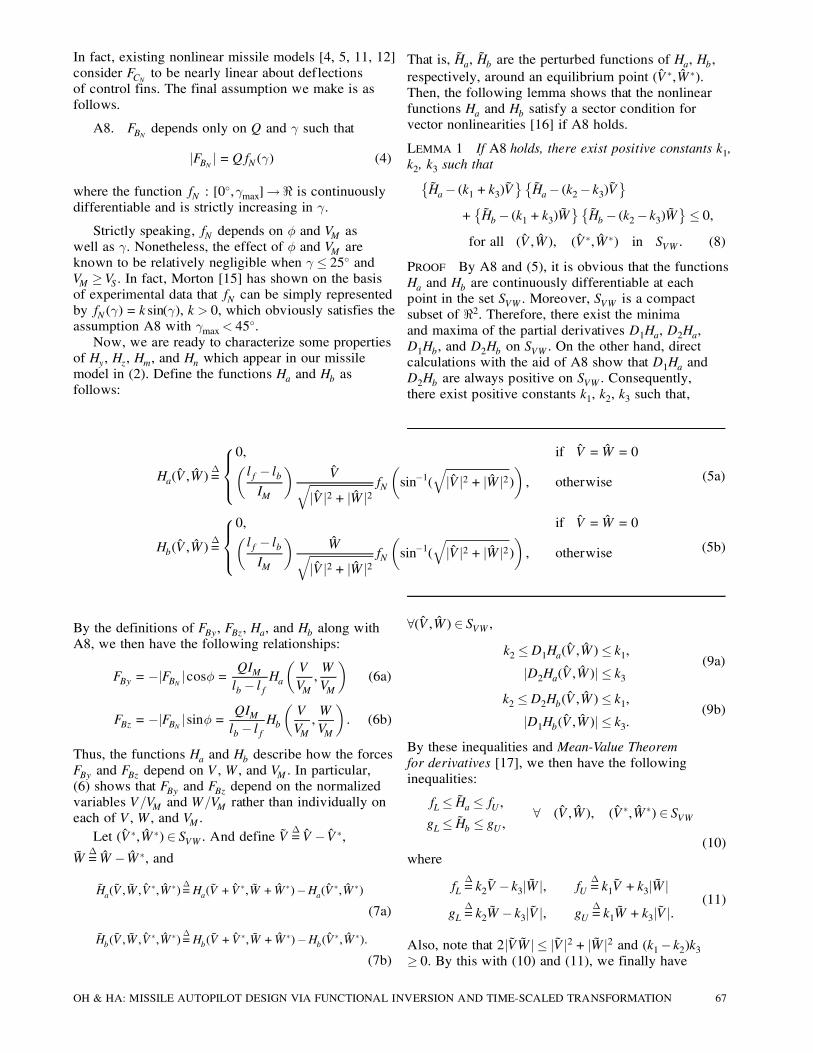
where I½ corresponds to the range of altitude from thesea level up to about 10 km.Some typical aerodata of the short-range

surface-to-air STT missile for which we attempt todesign an autopilot are plotted graphically in Fig. 4.For readability, we have described Hm and Hz in termsof ®, ¯, Á, and M. Fig. 4(a) shows that Hm is highlynonlinear about ®. In particular, the derivative ofHm with respect to ® changes its sign at about §5±and §10±. On the other hand, we see from Fig. 4(b)that Hz is invertible for ±q and hence that A7 issatisfied. Therefore, we can find the functions Kyand Kz in look-up table form, which satisfy (15). By

72 IEEE TRANSACTIONS ON AEROSPACE AND ELECTRONIC SYSTEMS VOL. 33, NO. 1 JANUARY 1997

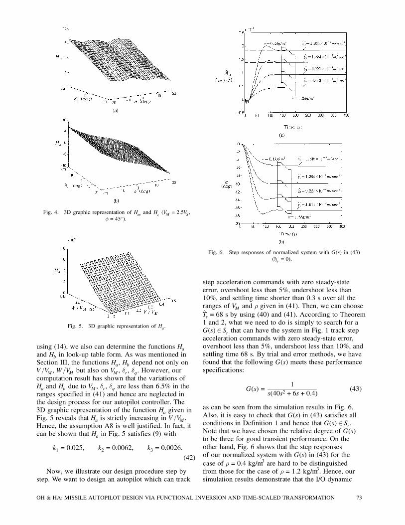
Fig. 4. 3D graphic representation of Hm and Hz (VM = 2:5VS ,Á= 45±).

Fig. 5. 3D graphic representation of Ha.

using (14), we also can determine the functions Haand Hb in look-up table form. As was mentioned inSection III, the functions Ha, Hb depend not only onV=VM , W=VM but also on VM , ±r, ±q. However, ourcomputation result has shown that the variations ofHa and Hb due to VM , ±r, ±q are less than 6.5% in theranges specified in (41) and hence are neglected inthe design process for our autopilot controller. The3D graphic representation of the function Ha given inFig. 5 reveals that Ha is strictly increasing in V=VM .Hence, the assumption A8 is well justified. In fact, itcan be shown that Ha in Fig. 5 satisfies (9) with

k1 = 0:025, k2 = 0:0062, k3 = 0:0026:

(42)

Now, we illustrate our design procedure step bystep. We want to design an autopilot which can track

Fig. 6. Step responses of normalized system with G(s) in (43)(ˆ y = 0).

step acceleration commands with zero steady-stateerror, overshoot less than 5%, undershoot less than10%, and settling time shorter than 0.3 s over all theranges of VM and ½ given in (41). Then, we can chooseTs = 68 s by using (40) and (41). According to Theorem1 and 2, what we need to do is simply to search for aG(s) 2 Sr that can have the system in Fig. 1 track stepacceleration commands with zero steady-state error,overshoot less than 5%, undershoot less than 10%, andsettling time 68 s. By trial and error methods, we havefound that the following G(s) meets these performancespecifications:

G(s) =1

s(40s2 +6s+0:4)(43)

as can be seen from the simulation results in Fig. 6.Also, it is easy to check that G(s) in (43) satisfies allconditions in Definition 1 and hence that G(s) 2 Sr.Note that we have chosen the relative degree of G(s)to be three for good transient performance. On theother hand, Fig. 6 shows that the step responsesof our normalized system with G(s) in (43) for thecase of ½= 0:4 kg/m3 are hard to be distinguishedfrom those for the case of ½= 1:2 kg/m3. Hence, oursimulation results demonstrate that the I/O dynamic

OH & HA: MISSILE AUTOPILOT DESIGN VIA FUNCTIONAL INVERSION AND TIME-SCALED TRANSFORMATION 73

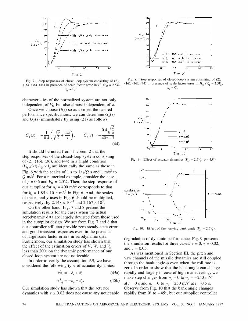
Fig. 7. Step responses of closed-loop system consisting of (2),(16), (36), (44) in presence of scale factor error in Hz (VM = 2:5VS ,

´y = 0).

characteristics of the normalized system are not onlyindependent of VM but also almost independent of ½.Once we choose G(s) so as to meet the desired

performance specifications, we can determine Go(s)and Gf(s) immediately by using (21) as follows:

Gf(s) =¡10:4

μr½

2+1:5s

¶, Go(s) =¡

0:4r2½

40s+7:

(44)

It should be noted from Theorem 2 that thestep responses of the closed-loop system consistingof (2), (16), (36), and (44) in a flight condition(VM ,½) 2 IVM £ I½ are identically the same as those inFig. 6 with the scales of 1 s to 1=

pQ s and 1 m/s2 to

Q m/s2. For a numerical example, consider the caseof ½= 0:6 and VM = 2:5VS . Then, the step response ofour autopilot for ´y = 400 m/s

2 corresponds to thatfor ˆy = 1:85£10¡3 m/s2 in Fig. 6. And, the scalesof the x- and y-axes in Fig. 6 should be multiplied,respectively, by 2:148£ 10¡3 and 2:167£ 105.On the other hand, Fig. 7 and 8 present the

simulation results for the cases when the actualaerodynamic data are largely deviated from those usedin the autopilot design. We see from Fig. 7 and 8 thatour controller still can provide zero steady-state errorand good transient responses even in the presenceof large scale factor errors in aerodynamic data.Furthermore, our simulation study has shown thatthe effect of the estimation errors of V, W, and VMless than 20% on the dynamic performance of ourclosed-loop system are not noticeable.In order to verify the assumption A9, we have

considered the following type of actuator dynamics:

¿ _±r =¡±r+ ±cr (45a)

¿ _±q =¡±q+ ±cq: (45b)

Our simulation study has shown that the actuatordynamics with ¿ · 0:02 does not cause any noticeable

Fig. 8. Step responses of closed-loop system consisting of (2),(16), (36), (44) in presence of scale factor error in Hm (VM = 2:5VS ,

´y = 0).

Fig. 9. Effect of actuator dynamics (VM = 2:5VS , Á= 45±).

Fig. 10. Effect of fast-varying bank angle (VM = 2:5VS).

degradation of dynamic performance. Fig. 9 presentsthe simulation results for three cases: ¿ = 0, ¿ = 0:02,and ¿ = 0:05.As was mentioned in Section III, the pitch and

yaw channels of the missile dynamics are still coupledthrough the bank angle Á even when the roll rate iszero. In order to show that the bank angle can changerapidly and largely in case of high maneuvering, wemake step changes from ´y = 0 to ´y =¡250 m/s2at t= 0 s and ´z = 0 to ´y = 250 m/s

2 at t = 0:5 s.Observe from Fig. 10 that the bank angle changesrapidly from 0± to ¡45±, but our autopilot controller

74 IEEE TRANSACTIONS ON AEROSPACE AND ELECTRONIC SYSTEMS VOL. 33, NO. 1 JANUARY 1997

still provides good set-point tracking performance,although some coupling occurs between pitch and yawchannels. This is because our approach to autopilotdesign takes the effect of the bank angle into account.Until now, we have assumed that VM and ½ are

constant. See A2. However, the recent stability analysison gain-scheduled system [6] or the well-knowntheoretical results on slow-varying systems [16] suggestthat our autopilot controller still will provide goodperformance if VM and ½ vary slowly comparedwith the autopilot dynamics. Finally, we verify thisthrough simulation. To this aim, we make a scenarioof flight path as is shown in Fig. 11(a), where VM and ½decrease at constant rate, respectively, from Mach 3 toMach 1.5 and from 1:2 kg/m3 to 0:4 kg/m3 in 4 s. Notethat along the flight path, Q decreases 1

12 times in 4 s.In this situation, a series of large step accelerationcommands as is shown in Fig. 11(b) is given to ourautopilot controller. As the result, the step commandsswing the angle of attack through a wide range as canbe seen from Fig. 11(c). In Fig. 11(b), we see that allperformance specifications are met even in such anill-conditioned flight situation. Hence, the simulationresults in Fig. 11 convince us that our approach toautopilot design provides not only a very simple butalso quite effective gain-scheduling procedure forrobust performance. It also suggests that our autopilotcontroller still can give good performance even inflight with the thrust burn in.

VI. CONCLUSIONS

In this paper, we have proposed a new approach toacceleration control of STT missiles and demonstratedits generality and practical use through stability analysisand simulation. Our autopilot controller may requirelarge memory to store the exact inversions of Hyand Hz in look-up table form. Please see (15). Thisproblem can be resolved easily due to the recentsemiconductor production technology. Moreover, oursimulation results shows that the effect of imperfectfunctional inversion on stability and performance isnot significant. The highlights in our approach are1) the very simple gain-scheduling procedure basedon the normalized system, and 2) the rigorous stabilityanalysis of our autopilot controller based on the fullnonlinear model for STT missiles.Nonetheless, some important issues still remain

untouched. For instance, we have assumed thatroll-stabilization is perfect. However, some rollrate is unavoidable in practice and can cause somefluctuation in missile acceleration. In order to reducefurther the effect of roll rate on the pitch and yawchannels, we may have to consider other types ofdynamic compensators. This issue is directly relatedto extension of our work to BTT missiles and needbe explored more extensively in future. On the otherhand, the sampling rate should be chosen carefully

Fig. 11. Step responses of closed-loop system consisting of (2),(16), (36), (44) for sequence of step commands (Acy(t) = 0 m/s

2).(a) Scenario of flight path (Mach number M, air density ½,dynamic pressure Q). (b) Acceleration. (c) Angle of attack.

in case of digital implementation of our autopilotcontroller. In fact, our simulation study for the caseof the practical example shows that a sampling rateslower than 1 kHz can cause some oscillation inacceleration responses. However, this can be expectedsince our autopilot is designed to have the settling timeless than 0.3 s in any flight condition.

REFERENCES

[1] Blakelock, J. H. (1991)Automatic Control of Aircraft and Missile.New York: Wiley, 1991.

OH & HA: MISSILE AUTOPILOT DESIGN VIA FUNCTIONAL INVERSION AND TIME-SCALED TRANSFORMATION 75

[2] Tahk, M., Briggs, M., and Menon, P. K. A. (1988)Application of a plant inversion via state feedback tomissile autopilot design.In Proceedings of IEEE Conference on Decision andControl, Austin, TX, Dec. 1988, 730—735.

[3] Reboulet, C., and Champetier, C. (1984)A new method for linearizing nonlinear systems: Thepseudolinearization.International Journal of Control, 40, 4 (Apr. 1984),631—638.

[4] Nichols, R. A., Reichert, R. T., and Rugh, W. J. (1993)Gain-scheduling for H-infinity controllers: A flight controlexample.IEEE Transactions on Control Systems Technology, 1, 2(June 1993), 69—79.

[5] Shamma, J. S., and Cloutier, J. R. (1993)Gain-scheduled missile autopilot design using linearparameter varying transformation.Journal of Guidance, Control, and Dynamics, 16, 2 (1993),256—263.

[6] Shamma, J. S., and Athans, M. (1990)Analysis of nonlinear gain-scheduled control systems.IEEE Transactions on Automatic Control (Aug. 1990),898—907.

[7] Isidori, A. (1989)Nonlinear Control System.Berlin: Springer-Verlag, 1989.

[8] Ha, I. J., and Chong, S. (1992)Design of a CLOS guidance law via feedback linearization.IEEE Transactions on Aerospace and Electronic Systems, 28(Jan. 1992), 51—62.

[9] Meyer, G., Su, R., and Hunt, L. R. (1984)Application of nonlinear transformations to automaticflight control.Automatica, 20 (1984), 103—107.

Jae-Hyuk Oh was born in Seoul, Korea, on September 9, 1966. He received theB.S., M.S., and Ph.D. degrees in control and instrumentation engineering fromSeoul National University, Seoul, Korea, in 1989, 1991, and 1996, respectively.He is presently a senior researcher at Automatic Control Research Center,

Seoul National University. His current field of interest is nonlinear control theoryand its applications to missile guidance and control.

In-Joong Ha received the Ph.D. degree in computer, information, and controlengineering (CICE) from the University of Michigan, Ann Arbor, in 1985.He is presently a Professor in the Department of Control and Instrumentation

Engineering, Seoul National University, Seoul, Korea. From 1973 to 1981, heworked in the area of missile guidance and control at the Agency of DefenseDevelopment in Korea. From 1982 to 1985, he was a Research Assistant atthe Center for Research on Integrated Manufacturing, University of Michigan,AnnArbor. From 1985 to 1986, he was with General Motors ResearchLaboratories, Troy, MI. His current research interest includes nonlinear controltheory and its applications to missiles, electric machines, and high precision servosystems for factory automation and multimedia.Dr. Ha was the recipient of the 1985 Outstanding Achievement Award in the

CICE program.

[10] Romano, J. J., and Singh, S. N. (1990)I-O map inversion, zero dynamics and flight control.IEEE Transactions on Aerospace and Electronic Systems, 26(Nov. 1990), 1022—1028.

[11] Huang, J., Lin, C. F., Cloutier, J.R., Evers, J. H., andD’Souza, C. (1992)Robust feedback linearization approach to autopilotdesign.IEEE Conference on Control Application, 1 (1992),220—225.

[12] Lin, C. F. (1994)Advanced Control Systems Design.Englewood Cliffs, NJ: PTR Prentice Hall, 1994.

[13] Marino, R. (1986)On the largest feedback linearizable subsystems.Systems and Control Letters, 6 (1986), 345—351.

[14] Respondek, W. (1986)Partial linearization, decomposition and fibre linearsystems.In Theory and Application of Nonlinear Control Systems.North-Holand, Elsevier, 1986, 137—154.

[15] Morton, B. (1992)A dynamic inversion control approach for high-machtrajectory tracking.In Proceedings of the American Control Conference,Chicago, IL, June 1992, 1332—1336.

[16] Khalil, H. K. (1992)Nonlinear Systems.New York: Macmillan, 1992.

[17] Apostol, T. M. (1974)Mathematical Analysis.Reading, MA: Addison-Wesley, 1974.

76 IEEE TRANSACTIONS ON AEROSPACE AND ELECTRONIC SYSTEMS VOL. 33, NO. 1 JANUARY 1997