Atmos. Meas. Tech., 7, 3387–3398, 2014www.atmos-meas-tech.net/7/3387/2014/doi:10.5194/amt-7-3387-2014© Author(s) 2014. CC Attribution 3.0 License.

Mirror contamination in space I: mirror modelling

J. M. Krijger 1, R. Snel1, G. van Harten2, J. H. H. Rietjens1, and I. Aben1

1SRON Netherlands Institute for Space Research, Sorbonnelaan 2, 3584CA Utrecht, the Netherlands2Leiden Observatory, Leiden University, Niels Bohrweg 2, 2333CA Leiden, the Netherlands

Correspondence to:J. M. Krijger (krijger@sron.nl)

Received: 16 December 2013 – Published in Atmos. Meas. Tech. Discuss.: 7 February 2014Revised: 27 June 2014 – Accepted: 9 July 2014 – Published: 7 October 2014

Abstract. We present a comprehensive model that can beemployed to describe and correct for degradation of (scan)mirrors and diffusers in satellite instruments that suffer fromchanging optical Ultraviolet to visible (UV–VIS) propertiesduring their operational lifetime. As trend studies becomemore important, so does the importance of understanding andcorrecting for this degradation. This is the case not only withrespect to the transmission of the optical components, butalso with respect to wavelength, polarisation, or scan-angleeffects. Our hypothesis is that mirrors in flight suffer from thedeposition of a thin absorbing layer of contaminant, whichslowly builds up over time. We describe this with the Muellermatrix formalism and Fresnel equations for thin multi-layercontamination films. Special care is taken to avoid the con-fusion often present in earlier publications concerning theMueller matrix calculus with out-of-plane reflections. Themethod can be applied to any UV–VIS satellite instrument.We illustrate and verify our approach to the optical behaviourof the multiple scan mirrors of SCIAMACHY (onboard EN-VISAT).

1 Introduction

Almost all optical instruments in space suffer from transmis-sion loss due to in-flight degradation of optical componentsand/or detectors. This transmission loss, especially at shorterUltraviolet (UV) wavelengths, can, in the worst case, causea nearly complete loss of detectable photons, and in lessercases a strong decrease in the signal-to-noise ratio. Often thistransmission loss is corrected by solar calibration, e.g. byusing a diffuser to observe the (assumed stable) sun. How-ever, instruments employing scan mirrors often observe theirscientific targets under different angles than their (in-flight)

calibration sources. As more satellites spent longer times inorbit, it became clear that the transmission loss or degra-dation is dependent on the scan angle (of the scan mirror)(Krijger et al., 2005b; Tilstra et al., 2012). This has been re-ferred to as the scan-angle-dependent degradation. This prob-lem is becoming more pressing with the increasing numberof long-term (climate) trend studies.

Our hypothesis is that both scan mirrors and surface dif-fusers suffer from a thin absorbing layer of contaminant,which slowly builds up over time. Many previous studies ofsuch contaminant layers that form on mirrors and/or diffusersin space have been performed. However, despite their goodquality, many authors decided not to publish in peer-reviewedscientific journals. Studies like e.g. the one byStiegman et al.(1993) on diffusers, show some organic effluent present, butdid not allow for the identification of the contaminant. Also,Chommeloux et al.(1998) showed the on-ground degrada-tion as a result of UV or photon radiation, as didGeorgievand Butler(2007) or Fuqua et al.(2004). In-flight studies ofcontaminant are of course more difficult. Some studies arecollected in an extensive database, which has recently beenmade available to the general public (Green, 2001). In sum-mary, most of the early satellites suffered from degradationcaused by outgassing. However, the exact identity of the con-taminant causing the Ultraviolet to visible (UV–VIS) degra-dation remained unclear.McMullin et al. (2002) studied thedegradation of SOHO/SEM, and found that they could ex-plain the degradation with a thin layer of carbon forming onthe forward aluminium filter. The exact source of the con-taminant is unknown, but is suspected to be outgassing of thesatellite itself.Schläppi et al.(2010) attempted in situ massspectrometry with ROSETTA to measure the constituents oftheir contamination, and found the main contaminants to bewater. In addition, organics from the spacecraft structure,

Published by Copernicus Publications on behalf of the European Geosciences Union.

3388 J. M. Krijger et al.: Mirror contamination I

electronics and insulations were identified. Water was alsofound in SCIAMACHY, where it was deposited onto the colddetectors (Lichtenberg et al., 2006). In fact, Earth-observingsatellites suffer from degradation, both in throughput andin the polarisation and/or scan-angle dependence, such asGOME (Krijger et al., 2005a; Slijkhuis et al., 2006), MODIS(Xiong et al., 2003; Xiong and Barnes, 2006; Meister andFranz, 2011), SeaWiFs (Eplee et al., 2007), VIIRS (Lei et al.,2012), MERIS (Delwart, 2010), SCIAMACHY (Bramstedtet al., 2009)1, and the two GOME-2 (Lang, 2012) instru-ments currently in orbit. Most provide an empirical degra-dation correction for the data users.

Thin layer deposits on mirrors and diffusers have beenmodelled before (e.g. most recently byLei et al., 2012); how-ever, these earlier attempts focus only on transmission loss,and often do not take scan-angle dependence into account,and none consider polarisation. These, however, need to beconsidered for a proper description of in-flight behaviour.This can be done by employing the Mueller matrix formalismand Fresnel equations. The application of Mueller matrix cal-culation in combination with the Fresnel equations requiresspecial care due to their different mathematical descriptionsof polarised light, especially in the case of out-of-plane re-flections. However, there are many ambiguities in often notwell-defined absolute polarisation frames, in the direction orhandedness in the often ignored circular polarisation, in nam-ing conventions, or in the application of signs with respect toframe changes, which often lead to much confusion. There-fore, in this paper, we go for the first time2 into full detail, andpresent a consistent, well-defined approach to Mueller ma-trix calculation in combination with Fresnel equations, usingdetailed illustrations and descriptions to describe the mathe-matics and frames. We will show that this approach is in fullagreement with verification measurements, and is generallyapplicable.

As the first paper in a planned series on in-flight mirrorcontamination, this initial paper focuses on the mathematicalmodelling of the mirror with possible contaminants. Furtherapplication to in-flight measurements and how to derive op-tical properties of in-flight contaminations will be presentedin a follow-up paper.

This study was initiated to investigate the wavelengthand scan-angle-dependent degradation as observed by SCIA-MACHY, onboard ENVISAT (Gottwald and Bovensmann,2011), which affects long-term data records. The optical be-haviour of the scan mirror of SCIAMACHY has been simu-lated based on this model, and was compared with measure-ments during on-ground calibration and dedicated laboratorymeasurements, which show that the model performs very sat-isfactorily under those early on-ground conditions. Analysesof in-flight SCIAMACHY contaminations and its behaviourover time will also be presented in a follow-up paper.

1Data athttp://www.iup.uni-bremen.de/sciamachy/mfactors/.2To the authors’ knowledge.

The great value of this model is that it is generally ap-plicable and can easily be applied to all satellites, employing(scan) mirrors or other reflecting optics suffering from degra-dation due to contamination. The model, once applied, canprovide detailed scan-angle and wavelength behaviour as afunction of time, allowing for accurate correction, which isneeded for precise (trend) analyses.

In Sect.2, we describe a model for a scan mirror and a sur-face diffuser. In Sect.3, we shortly describe SCIAMACHY,important for our verification. This verification using on-ground measurements is described in Sect.4. A general dis-cussion follows. Finally, we will draw conclusions on themodel with an outlook to its application.

2 Model

2.1 Mueller calculus

In order to model the scan-angle-dependent throughput ofmirrors, we employ the well-known Stokes and Mueller cal-culus (Azzam and Bashara, 1987; Hecht, 1987). The incom-ing (partly) polarised light is characterised by a Stokes vectorI

I =

I

Q

U

V

, (1)

Here, I is the intensity, Q and U describe the two-dimensional state of linear polarisation, andV represents cir-cular polarisation.

Any description of polarisation requires an exact refer-ence frame definition. In this paper, we use the same refer-ence frame and conventions asHecht(1987). This means thatwhen looking along the direction in which the light is travel-ling, positiveU is found by rotating 45◦ anticlockwise fromQ, while positiveV is defined when theE vector is rotatingclockwise, as shown in Fig.1. Note that the rotation and di-rection of theE vector is defined in a fixed reference frameor plane. Many other frame definitions are in use; however,these will require different Mueller matrices than those usedin this text.

The Stokes vectorI is often split into a total signal partand a polarisation vector,

I = I0 ·

1q

u

v

, (2)

with q, u, andv the fractional polarisationQ, U , andV withrespect to the total signal,I0.

Any detected signalS depends on the received polarisedlight I and the polarisation sensitivity of the instrumentµ,

S = µ · I , (3)

Atmos. Meas. Tech., 7, 3387–3398, 2014 www.atmos-meas-tech.net/7/3387/2014/

J. M. Krijger et al.: Mirror contamination I 3389

Figure 1. Stokes vector frame definition used in the paper. Pointingvector is perpendicular and into the paper (following the light).

with

µ = M1 · (1,µ2,µ3,µ4), (4)

with M1 the absolute radiance sensitivity of the instrumentandµx the normalised polarisation sensitivity ofq, u, andv

of the instrument, respectively.Any optical element that modifies the polarised light, such

as retarders, polarisers, and mirrors, can be described as a 4×

4 transformation matrixM (known as the Mueller matrix):

S = µ · M · I . (5)

For polarisation-insensitive detectors, the first row ofMis often considered equivalent toµ, thus removing the needfor µ. However, here we consider a possible polarisation-sensitive instrument, and choose to employµ explicitly.

Multiple elements encountered by the light can be de-scribed by multiplying consecutive Mueller matrices:

S = µ · Mn. . .M3M2M1 · I . (6)

Note that, for Mueller matrix calculations, the first encoun-tered element by the light is the one farthest right in the for-mula. Matrix multiplication is not commutative, so order isimportant.

It is always important to define the reference frame both atthe detector and at the source, and to keep track of the frameat different positions between source and detector, since aframe rotation might be needed between two optical com-ponents when out-of-plane reflections happen. In reflections,thep ands directions are often used. Thep polarisation (pfrom “parallel”) is the polarisation in the plane of reflectionor incidence, whiles polarisation (s from “senkrecht”, Ger-man for perpendicular) is perpendicular to this plane (see

Figure 2. s andp polarisation direction definitions for a reflection.

Fig. 2). The p and s frame can be, and often is, coupledto a Stokes frame in the case of a single reflection, withS ≡ Q = 1 andP ≡ Q = −1. However, this is a choice andcan be different, as long as the Stokes frame is rotated be-fore and after a reflection to thep ands frame (see Sect.2.5for more details on frame rotations). For example, the mirrorin Fig. 2 would have to be rotated 90◦ in order to match theframe from Fig.1 with S ≡ Q = 1.

2.2 Mirror model

The generic Mueller matrix for a mirror, defined in the refer-ence frame of Fig.1, with the angle of incidence of the lightgiven byimir and the plane of reflection perpendicular to theQ = 1 direction, is given byAzzam and Bashara(1987):

Mmir(φmir) =12 (r2

s + r2p) 1

2 (r2s − r2

p) 0 012 (r2

s − r2p) 1

2 (r2s + r2

p) 0 00 0 |rp ||rs |cos(1) |rp ||rs |sin(1)0 0 −|rp ||rs |sin(1) |rp ||rs |cos(1)

,(7)

where the complex reflection coefficientsrp andrs for s- andp-polarised light are given by the Fresnel equations

rp =

n2cos(φmir) − n1

√1−

(n1n2

sin(φmir))2

n2cos(φmir) + n1

√1−

(n1n2

sin(φmir))2

, (8)

rs =

n1cos(φmir) − n2

√1−

(n1n2

sin(φmir))2

n1cos(φmir) + n2

√1−

(n1n2

sin(φmir))2

. (9)

The complex indices of refraction of the mirror materialand ambient medium are denoted byn2 andn1. Note thatn = nr − ik, with k ≥ 0, with nr the real part andk the imag-inary part. This makesk a damping factor, which describesthe absorption of light by metals (seevan Harten et al., 2009).Note that thes andp directions are given here according tothe conventional definition, withp in the plane of reflection

www.atmos-meas-tech.net/7/3387/2014/ Atmos. Meas. Tech., 7, 3387–3398, 2014

3390 J. M. Krijger et al.: Mirror contamination I

ands perpendicular to this plane. The phase jump1 in thiscoordinate frame is defined as

1 = arg(rp) − arg(rs). (10)

On a side note: a perfect reflection is described by

Mperfect reflection=

1 0 0 00 1 0 00 0 −1 00 0 0 −1

. (11)

The reflection Mueller matrix correctly describes that thesigns ofU andV flip. This is a direct consequence of thefact that the Stokes frame is defined for an observer look-ing along the beam, so upon reflection, the definitions of leftand right are swapped. This sign change ofU andV can beachieved mathematically by changing the signs in the lower-right quadrant of the mirror Mueller matrix (see e.g.Keller,2002), or as was done here, by the definition of1 with rpandrs , which cause a 180◦ phase difference for a perfect re-flection.

2.3 Diffuser model

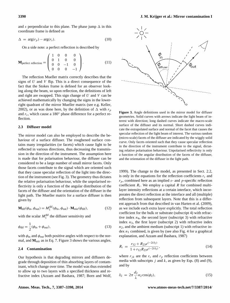
The mirror model can also be employed to describe the be-haviour of a surface diffuser. The roughened surface con-tains many irregularities (or facets) which cause light to bereflected in various directions, thus decreasing the transmis-sion in the direction of the instrument. The assumption hereis made that for polarisation behaviour, the diffuser can beconsidered to be a large number of small mirror facets. Onlythose facets contribute to the signal which are oriented suchthat they cause specular reflection of the light into the direc-tion of the instrument (see Fig.3). The geometry thus dictatesthe relative polarisation behaviour, while the unpolarised re-flectivity is only a function of the angular distribution of thefacets of the diffuser and the orientation of the diffuser in thelight path. The Mueller matrix for a surface diffuser is thengiven by

Mdif(φin,φout) = Mdif1 (φin,φout) · Mmir(φdif), (12)

with the scalarMdif1 the diffuser sensitivity and

φdif =1

2(φin + φout), (13)

with φin andφout both positive angles with respect to the nor-mal, andMmir as in Eq.7. Figure3 shows the various angles.

2.4 Contamination

Our hypothesis is that degrading mirrors and diffusers de-grade through deposition of thin absorbing layers of contam-inant, which change over time. The model was thus extendedto allow up to two layers with a specified thickness and re-fractive index (Azzam and Bashara, 1987; Born and Wolf,

Figure 3. Angle definitions used in the mirror model for diffusergeometries. Solid curves with arrows indicate the light beam of in-terest with direction; long dashed curves indicate the macro-scalesurface of the diffuser and its normal. Short dashed curves indi-cate the extrapolated surface and normal of the facet that causes thespecular reflection of the light beam of interest. The various random(micro-scale) facets of the diffuser are indicated by the wiggly solidcurve. Only facets oriented such that they cause specular reflectionin the direction of the instrument contribute to the signal, dictat-ing relative polarisation behaviour. Unpolarised reflectivity is onlya function of the angular distribution of the facets of the diffuser,and the orientation of the diffuser in the light path.

1999). The change to the model, as presented in Sect.2.2,is only in the equations for the reflection coefficientsrs andrp, combined here as an implieds- andp-specific reflectioncoefficientRt . We employ a capitalR for combined multi-layer intensity reflections at a certain interface, which incor-porates the direct reflection at the interface and all (multiple)reflection from subsequent layers. Note that this is a differ-ent approach from that described invan Harten et al.(2009),as we include each extra layer explicitly. The total reflectioncoefficient for the bulk or substrate (subscript 4) with refrac-tive indexn4, the second layer (subscript 3) with refractiveindex n3, the first layer (subscript 2) with refractive indexn2, and the ambient medium (subscript 1) with refractive in-dexn1 combined, is given by (see also Fig.4 for a graphicalexplanation, and Azzam and Bashara, 1987)

Rt =r12+ R23e

(−2iδ2)

1+ r12R23e(−2iδ2), (14)

whererjk are thers and rp reflection coefficients betweenmedia with subscriptsj andk, as given by Eqs. (8) and (9),and by

δ2 = 2πd2

λn2cos(φ2), (15)

Atmos. Meas. Tech., 7, 3387–3398, 2014 www.atmos-meas-tech.net/7/3387/2014/

J. M. Krijger et al.: Mirror contamination I 3391

Figure 4. Layers and angle definitions used in the mirror modelwith thickness (di ) and complex refractive index (ni ). Left: annota-tion for the general case; right: materials for SCIAMACHY appli-cation.

cos(φ2) =

√1−

(n1

n2sin(φ1)

)2

, (16)

R23 =r23+ r34e

(−2iδ3)

1+ r23r34e(−2iδ3). (17)

δ3 = 2πd3

λn3cos(φ3), (18)

cos(φ3) =

√1−

(n2

n3sin(φ2)

)2

=

√1−

(n1

n3sin(φ1)

)2

, (19)

with φx the angle of incidence in mediumx (only φ1 isneeded; the others can be derived as shown),λ the wave-length of the light, andd2 and d3 the layer thicknesses ofthe layers closest to the ambient medium and the substrate,respectively.

To expand the model to any desired number of layers, thetotal reflectanceRt at the top interface of a multi-layer systemcan be calculated by determining the combined (multi-layer)reflectance at the interface between the ambient medium(subscript 1) and the first layer (index 2),R12, as done inEq. (14). However, Eq. (17) must be expanded to the gen-eral case, where the combined (multi-layer) reflectance atthe interface between layer or mediumi and layerj (withj = i + 1), namelyRi,j , is given by

Ri,j =ri,j + Rj,j+1e

(−2iδj )

1+ ri,jRj,j+1e(−2iδj )

, (20)

with

δj = 2πdj

λnj cos(φj ), (21)

cos(φj ) =

√1−

(ni

nj

sin(φi)

)2

. (22)

R12 can thus be calculated by successively employingEq. (20)–(22) for incrementing layersi and j until an ef-fectively infinite layern + 1 (whereRn,n+1 = rn,n+1, as inEq.17) or the desired accuracy is reached.

2.5 Multiple mirrors

Some instruments, such as SCIAMACHY, employ multiplescan mirrors. As a result, both polarisation and throughputchange as a function of the viewing angle of each mirror.The modelling of the reflection from multiple mirrors mayrequire the use of rotation matrices. Especially in cases wherethe planes of two successive reflections are not parallel, arotation of the reference frame is needed in order to align theQ = 1 direction of the reference frame with thes directioncorresponding to the plane of reflection. The rotation matrixover an arbitrary angleγ is given by

R(γ ) =

1 0 0 00 cos(2γ ) −sin(2γ ) 00 sin(2γ ) cos(2γ ) 00 0 0 1

. (23)

Using this Mueller matrix withγ = 45◦ changesQ = 1into U = 1. In order to add an optical element with Muellermatrix M placed at an angleγ , one has to rotate the elementmathematically in line as follows, to get it to align with ourframe:

M rot = R(γ ) · M · R(−γ ). (24)

For a mirror, where the reflection flips the coordinates, theback transformation should hence also be mirrored (Keller,2002), resulting in

M rot = R(−γ ) · M · R(−γ ). (25)

For clarity, note that all rotation signs can be swapped aslong as they are then also changed in the rotation matrix.Sometimes both definitions are used in the same book, e.g.in Azzam and Bashara(1987). Note that for polarisation, twopositive rotations do not equal two negative rotations, due tothe handedness of polarisation.

Combining the two mirrors can then be written as

Mmir(φmir1,φmir2) =

R(−γmir2) · M(φmir2) · R(−γmir2)

· R(−γmir1) · M(φmir1) · R(−γmir1). (26)

www.atmos-meas-tech.net/7/3387/2014/ Atmos. Meas. Tech., 7, 3387–3398, 2014

3392 J. M. Krijger et al.: Mirror contamination I

Each rotation is with respect to the Stokes frame of thelight incident on the optical element. This allows changingfrom e.g. an external frame to an instrument frame and viceversa by adding the appropriate rotation matrix. When em-ploying two mirrors, the angle of incidence on the secondmirror depends on the angles at which the mirrors are rotatedwith respect to each other. An example of modelling two mir-rors applied to the case of SCIAMACHY will be shown inthe next section.

3 SCIAMACHY

The SCIAMACHY (Gottwald et al., 2006) calibration con-cept (Noël et al., 2003) builds on a combination of on-groundand in-flight calibration measurements. The on-ground cali-bration measurements were split up into ambient measure-ments comprising the scanner unit only, and thermal vac-uum (TV) measurements using the entire instrument. View-ing angle dependence for the on-ground calibration data isderived from the ambient measurements, while the remain-der of the calibration information is derived from the TVmeasurements. For in-flight conditions, the combination ofambient and TV data is essential.

Unforeseen instrumental polarisation behaviour, mostlikely caused by thermally induced stress birefringence ofone of the optical components in the instrument (Snel, 2000),required the initial calibration approach to be extended, withadditional on-ground polarisation characterisation of the in-strument.

Shortly after launch, discrepancies between the observedand expected signals were observed, and subsequently signif-icantly reduced by means of ad hoc sign changes of selectedpolarisation calibration parameters. This solution was con-sidered acceptable for the time being, and worked well fornadir viewing geometry, but needed additional workaroundsfor limb geometry. Here however we will now employ amore fundamental approach. Our method is consistent inboth nadir and limb, as we now describe the various mirrorsin the same frame.

3.1 SCIAMACHY mirrors

Aluminium mirrors are known to induce instrumental polari-sation when used at non-normal incidence (e.g.Thiessen andBroglia, 1959). Such mirrors however are often used in tele-scope mirrors, as onboard SCIAMACHY. This phenomenonis caused by differential reflection between polarisation inthe plane of incidence and polarisation perpendicular to it, asdescribed by the Fresnel equations. The amount of polarisa-tion depends on the mirror material, angle of incidence, andwavelength. For instance, reflection off an aluminium mirrorat 45◦ turns unpolarised visible light into 3 to 4 % polari-sation perpendicular to the plane of incidence (van Hartenet al., 2009).

It has been shown that these polarisation properties can notbe described using the Fresnel equations for bare aluminium(Burge and Bennett, 1964). Attempts to fit measured instru-mental polarisation to an aluminium model lead to unrealis-tic pseudo-indices of refraction (Sankarasubramanian et al.,1999; Joos et al., 2008).

Indeed, this bare aluminium model is incomplete, since theinstant an aluminium mirror is exposed to air, an aluminiumoxide layer a few nanometers thick starts growing on its sur-face. This phenomenon, as explained theoretically byMott(1939), was measured using microscopy and spectroscopyby Jeurgens et al.(2002). Mueller matrix ellipsometry byvanHarten et al.(2009) showed that the mirror polarisation canbe described by a∼ 4.12±0.08 nm aluminium oxide layer ontop of bulk aluminium, where the layer grows asymptoticallyto the final thickness within the first∼ 10 days. This is alsoneeded to describe the aluminium mirrors in SCIAMACHYadequately.

3.2 SCIAMACHY geometry

The SCIAMACHY scanner (Fig.5) consists of two mecha-nisms, each containing a mirror with a diffuser on the back.The elevation scan mirror (ESM) is needed for all measure-ment modes and contains the main diffuser. The azimuthscan mirror (ASM) is only used in limb measurement mode,including the Sun over ESM diffuser mode. The ESM andASM can be set at any angle.

SCIAMACHY has a geometry where detector and bothmirrors are in the same plane, but with a perpendicular ro-tation axis (see Fig.5). Let αx be the rotation of mirrorxaround its axis, with 45◦ mirror rotation resulting in the lightbeing reflected at 90◦. For the ESM (employed for both thenadir and limb scans), the angle of incidence towards the de-tector is equal to the rotation of the ESM on its axis:

φESM = αESM. (27)

When choosing the Stokes reference frames optimally(namelyS ≡ Q = 1 for the ESM), the nadir case is very sim-ple:

Moptnadir = M(φESM). (28)

For limb observations, the situation is a bit more compli-cated, because one has to account for the different orientationof the planes of reflection of the ESM and ASM with respectto the Stokes reference frames of the incoming and outgoinglight. The rotation angle between the plane of reflection ofthe ESM and the ASM is given by

γASM→ESM = π/2+ arcsin(cot(φmir1) · tan(2φmir2)). (29)

Also, the ASM must be placed at a very specific angle inorder to reflect the light onto the ESM and then the detec-tor/instrument slit. The required angle of incidence on the

Atmos. Meas. Tech., 7, 3387–3398, 2014 www.atmos-meas-tech.net/7/3387/2014/

J. M. Krijger et al.: Mirror contamination I 3393

Figure 5. Schematic view of SCIAMACHY multiple mirror setupin limb observation mode. On the left side, the Optical Bench Mod-ule (OBM) and entrance slit. On the right side, the ESM, which ifrotated to a 45◦ angle will reflect light (curve with arrow head) com-ing from below (nadir) directly into the slit. In the middle, the ASM,which reflects the (limb) light coming from the front and slightlybelow onto the ESM. Both mirrors have a bead-blasted aluminiumsurface diffuser on their back side (not shown here).

ASM can be calculated using

φASM = arccos(cos(αASM) · cos(2αESM)). (30)

The total Mueller matrix for limb observations is thengiven by

Moptlimb = M(φESM) · R(−γASM→ESM)

· M(φASM) · R(−γASM→ESM). (31)

However, for historical reasons, theQ = 1 direction waschosen perpendicular to the entrance slit of SCIAMACHY(see Fig.5), i.e. parallel to the scattering plane of the ESM,or 90◦ compared to the simple case. This requires several ro-tations, resulting in a Mueller matrix for nadir observations:

Mhistnadir = R(−γESM) · M(φESM) · R(−γESM), (32)

with γESM = 90◦.The total Mueller matrix for limb observations derived by

frame rotating for each mirror element is then given by

Mhistlimb = R(−γESM) · M(φESM) · R(−γESM)

· R(−γESM) · R(−γASM→ESM) · M(φASM)

· R(−γASM→ESM) · R(−γESM). (33)

As rotations are commutative, and two 90◦ rotations equala full rotation for polarisation, this equation can be simplifiedhere to

Mhistlimb = R(−γESM) · M(φESM) · R(−γESM)

· R(−γASM) · M(φASM) · R(−γASM), (34)

with

γASM = arcsin(cot(φmir1) · tan(2φmir2)). (35)

Finally, we emphasise that these formulas will change ifdifferent Stokes reference frames are used, but the approachremains the same.

4 Verification

Combining Mueller matrix formalism with the Fresnel equa-tions requires, especially in the case of out-of-plane reflec-tions, a precise definition and bookkeeping of mathematicalsigns and conventions. In particular, this applies to the ab-solute polarisation frame, to the rotations between framesbefore and after reflection, to the handedness of circularlypolarised light, and to the implementation in the form of analgorithm.

Hence, it is of the utmost importance to verify Muellermatrix calculations. In this section, we apply our model toSCIAMACHY on-ground measurements of the diffuser andscan mirrors. We show that all data can be explained well byusing Mueller matrix calculations in combination with theFresnel equations, confirming the correct use of these tools.

4.1 Refractive index

In the section below, we compare model calculations witholder on-ground measurements performed on aluminiummirrors during SCIAMACHY calibration. As mentioned,these aluminium mirrors were not vacuum protected, andwill thus have a thin layer of aluminium oxide on them.In order to describe these mirrors, the refractive index ofaluminium and aluminium oxide is needed for the wave-length range of interest (here 300–2400 nm). However, thereare several conflicting aluminium refractive indices availablein the literature, namely the direct measurements found inHaynes(2013) and Palik (1985) and the Kramers–Kronig-derived values ofRakic(1995). While the differences in therefractive index can be several percent, the difference in spe-cific applications is much harder to quantify. Our verificationresults improved very slightly when employing the indicesof Rakic (1995), and hence the choice was made to employthese indices.

To the best of our knowledge, in the literature there is nocomplete information on the refractive index of amorphousaluminium oxide in the 0.2–2.4 µm wavelength range.

However, the work ofEdlou et al.(1993) can be extrap-olated to the desired wavelength range by using the Cauchydispersion equation

n(λ) = A + Bλ−2+ Cλ−4. (36)

We employ the values found byEdlou et al.(1993) of 1.63,2.25×103 nm2, and 20.16×107 nm4 for A, B andC, respec-tively. The two different methods produce the same refractiveindices for aluminium oxide within uncertainties. The latteroption was employed for its ability to interpolate accuratelyto desired wavelengths.

4.2 Mirror model verification

First we compared the mirror model with the measurementsof van Harten et al.(2009). Shown in Fig.6 is the compar-ison at 600 nm, using a refractive index for the aluminium

www.atmos-meas-tech.net/7/3387/2014/ Atmos. Meas. Tech., 7, 3387–3398, 2014

3394 J. M. Krijger et al.: Mirror contamination I

Figure 6. Normalised Mueller matrix of reflection off a real aluminium mirror with an aluminium oxide layer of measured 4.1 nm on top ofit at 600 nm. Measurements by van Harten et al. (2009) (diamonds) and our model (lines).

of 1.262− i7.186 and a refractive index for the aluminiumoxide, calculated by Eq. (36), of 1.637− i0.000 at the mea-sured wavelength of 600 nm, for the different Mueller matrixcomponents. The normalised, to the top-left element, mea-surements are assumed to be accurate within 0.02. The first-column components, the instrumental polarisation sensitivityhere, has residuals smaller than 0.003, and are thus in al-most perfect agreement. The diagonal components, indicat-ing the transmission of polarisation, have residuals smallerthan 0.01. Other (polarisation cross-talk) residuals remainbelow 0.02, but here the measurements might have sufferedfrom limited calibration accuracy (for more discussion onthe measurements, seevan Harten et al., 2009). In summary,the residuals between measurement and model are withinthe measurement accuracy, hence the measurement data andmodel are in excellent agreement.

For another verification, we turned to SCIAMACHY. Dur-ing on-ground calibration of the SCIAMACHY aluminiumscan mirrors, reflectivity was measured with different polar-isation orientations of the incoming light, with both singleand multiple mirrors.

We show the most complicated situation first, with multi-ple mirrors where multiple orientations of linear polarisation(Q = 1, Q = −1, U = 1, andU = −1 with respect to theSCIAMACHY reference frame) were reflected on the wholescanner unit. The reflected light was then analysed by em-ploying linear polarisation filters (eitherQ = 1 or Q = −1).Shown in Fig.7 are both measurement and model simu-lations under the SCIAMACHY reference viewing angles(φESM = 12.7◦ and φASM = 45◦) for the various combina-tions of offered and measured polarisation directions. Theoriginal estimated errors bars are shown; however, alreadyduring the measurements, it was clear these were too opti-mistic (Dobber, 1999). As can be seen, the measurementsoriginally differed several standard deviations from a sim-ple clean mirror model employing the literature value for the

refractive index of aluminium. Including a 4.12 nm layer ofaluminium oxide (van Harten et al., 2009) improves the com-parison significantly; however, for the shortest wavelength,an additional contamination was needed. A correction by in-creasing the thickness of the aluminium oxide to 9 nm (notshown) showed improvement, but did not show the correctwavelength behaviour, and was rejected. Further investiga-tion showed that employing 0.4 nm of light oil contaminationon the surface of the mirrors would be consistent in order tomodel the measurements correctly.

The light oil optical properties were taken fromBarbaroet al. (1991). Such a small contamination of 0.4 nm on themirror was within the molecular cleanliness control require-ments (van Roermund, 1996) during on-ground measure-ments. Of course, the exact kind of oil or even the kind ofcontaminant is unknown; however, the assumption of lightoil contamination is not unreasonable. As both mirrors werekept under similar conditions, we assume a similar contami-nation of oil on both.

The good agreement between measurements and modelclearly shows that the mirror model works very well, andthat the inclusion of aluminium oxide and oil contaminationis necessary for explaining the measurement results. Sincean error or sign change in one of the rotation angles used inthe calculation will result in completely different polarisationsensitivities (not shown here), Fig.7 confirms that the correctsigns and rotation angles are employed. The use of the opticalproperties of light oil, while the true contaminant source andits polarisation properties are as yet unknown, could be thereason for the differences at the shortest wavelengths. How-ever, more likely the measurements have larger uncertaintiesthan originally stated.

The single mirror measurements are less sensitive to con-taminations, and are thus less useful for verification, but weshow them here for completeness in Fig.8. Again, a 4.1 nmaluminium oxide and 0.4 nm light oil contamination were

Atmos. Meas. Tech., 7, 3387–3398, 2014 www.atmos-meas-tech.net/7/3387/2014/

J. M. Krijger et al.: Mirror contamination I 3395

Figure 7. SCIAMACHY scan mirror reflectance for different po-larisation states of the incident light (Q = 1, Q = −1, U = 1, andU = −1 with respect to the SCIAMACHY reference frame) anddifferent orientation of the analysers (Q = 1 andQ = −1), as in-dicated in the subplots. The measurement results with error barsobtained during on-ground calibration are shown in red, while themodel calculations are represented by the black solid curve. Themodel calculation includes an aluminium mirror with 4.1 nm alu-minium oxide and 0.4 nm light oil contamination, and angles of in-cidenceφESM = 12.7◦ and φASM = 45◦. Dash–dotted curves in-dicate clean aluminium, and dotted curves aluminium with only4.1 nm aluminium oxide, as a comparison.

employed in order to employ identical mirrors, as for themultiple mirror case. Measurement and model are in goodagreement.

In order to verify the coordinate frames, to verify the em-ployed Mueller matrices, and to avoid previous on-groundconfusion, the authors have rebuilt the SCIAMACHY scan-ner setup in an optics lab. No new results where found, but allthe measurements confirmed all rotations and Mueller matrixsigns.

4.3 Diffuser model verification

The assumption that the diffuser acts as a surface diffuserwith mirror facets can be checked by changing the angle ofthe mirror with respect to a fixed light source and a fixed de-tector. In this case,φdif is fixed as the sum of the incident an-gle and the outgoing angle, which is the fixed angle betweenthe light source and the instrument. SinceMmir depends onlyon the fixedφdif , only the scalarMdif

1 (φin,φout) will vary dueto the change in the angle of incidence and the outgoing an-gle (see Eq.12). This will cause a change in the intensity ofthe signal, but not in the polarisation properties. Hence, therelative polarisation should remain the same in this situation,irrespective of the angle with respect to the fixed light sourceand the fixed detector.

A measurement to test this hypothesis has been performedon-ground for SCIAMACHY. A scan over 40◦ rotation of the

Figure 8. SCIAMACHY scan mirror reflectance for different po-larisations (S andP ; i.e. Q = 1 andQ = −1) of the incident lightand for different incident angles. Measurements during on-groundcalibration are shown as diamonds. The curves represent the re-flectance according to the mirror model, using an aluminium mirrorwith 4.1 nm aluminium oxide and 0.4 nm light oil contamination,under an angle of incidence of either 29◦ (dashed) or 61◦ (solid).Dotted and dash–dotted curves indicate the reflectance of clean alu-minium instead as a comparison.

mirror was made, while keeping the light source and detec-tor at a fixed position, over which a negligible change in po-larisation was observed during the measurements. In Fig.9,this is shown for a smaller range of rotation angles, near theoperational rotation angle of 165◦. In the figure, the mea-sured signal of the main science detectors for boths (Q = 1)andp polarisation (Q = −1) are plotted at 324 nm as a func-tion of the diffuser rotation angle. Both signals are scaled tothe maximum ofs polarisation for comparison, as the levelof the signals is a scanner-independent instrument character-istic, depending on the instrument polarisation sensitivities.The signals show exactly the same response (within the er-ror bars), as shown by their plotted ratio, indicating that thepolarisation did not change, only the total reflectance, as ex-pected.

5 Discussion

We present here a method capable of describing the degrada-tion as a function of wavelength, polarisation and scan anglefor all Earth-observing instruments employing a (scan) mir-ror in both low and geostationary orbits. In addition, employ-ing a time-dependent contaminant layer thickness also allowsus to describe the degradation as a function of time. Ini-tially this work was started to solve the scan-angle-dependentdegradation of SCIAMACHY, but in this paper we have at-tempted to describe the method in the most generic way, foreasy application to other instruments. Not all possible caseshave been described, but expansion of the model to for exam-ple more mirrors or layers can easily be derived from the pre-sented cases. The model is of interest to all instruments em-ploying (scan) mirrors or other optics suffering from degra-dation due to contamination. In its current version, the modelcan be applied to provide detailed scan-angle and wavelength

www.atmos-meas-tech.net/7/3387/2014/ Atmos. Meas. Tech., 7, 3387–3398, 2014

3396 J. M. Krijger et al.: Mirror contamination I

Figure 9. Diffuser model verification: scaled measured SCIA-MACHY signal of the main science detectors as a function of thecommanded diffuser angle for boths (Q = 1) andp polarisation(Q = −1) at 324 nm. Estimated uncertainties or noise (1σ ) are in-dicated by the filled yellow areas. As expected, the ratio betweens

andp polarisation (green curve) does not change as a function ofthe diffuser angle.

behaviour as a function of time, allowing for accurate cor-rection, which is needed for precise (trend) analyses. We willfurther expand on this and illustrate it by the application toSCIAMACHY in-flight measurements in the next paper inthis series.

For application to in-flight satellites, several propertiesmust be known: the instrument response to polarisation, themirror’s optical properties (along with its initial contamina-tions), and the in-flight contaminant optical properties. Themodel is not wavelength limited, as long as the optical prop-erties of the mirror are known for the wavelength of interest.Issues like a low signal or other instrument limitations willbe the limiting factor for the application of the model. Thein-flight contaminant optical properties especially are oftenunknown, and assumptions will have to be made. In the nextpaper in the series, we will present how this can be done forSCIAMACHY.

We have verified all assumptions and models, and thus re-moved any remaining sign or frame inconsistencies. All for-mulae and verification results are fully consistent with eachother. In previous measurements for, e.g., SCIAMACHY(Gottwald and Bovensmann, 2011), different mirror config-urations were taken as completely different measurementsin sometimes conflicting or partially defined polarisationframes. The current model always employs a well-definedframe with a consistent mathematical Mueller approach. Allof these frame definitions and approaches have been usedconsistently for all verification measurements. With this ap-proach, we were able to describe all the measurements avail-able to us. More proof of the correctness of the assumptionsor approach employed will follow in a future paper in the se-ries, where we will show the model as also describing time-dependent in-flight measurement behaviour.

6 Conclusions

We have presented a model for accurately describing reflec-tion and polarisation properties of multiple scan mirrors anddiffusers in space. This model includes the impact of contam-ination, both spectrally and scan angle dependent. The modelcan easily be applied to any satellite, both in low and geo-stationary orbits, employing (scan) mirrors or other opticssuffering from degradation due to contamination. Also, incases where no scan-angle-dependent degradation is present,but only wavelength-dependent degradation, the model al-lows for accurate in-flight corrections, provided that infor-mation on the contamination can be constrained. Our hy-pothesis is that both scan mirrors and diffusers suffer froma thin absorbing layer of contaminant, which slowly buildsup over time. We described this transmission, polarisationand angle dependence of mirrors, including multi-layers us-ing the Mueller matrix formalism and Fresnel equations. Inthis paper, we have gone into explicit detail with respect tothe handedness of the polarisation and mathematical signs,accompanied by detailed illustrations and descriptions. Weresolve the long-standing ambiguities in the application ofMueller matrix and Fresnel calculations in (out-of-plane) re-flections. As an application, the SCIAMACHY scanner hasbeen modelled based on this multiple-layer contaminatedmirror hypothesis. The model was checked against all knownon-ground measurements, and shows excellent agreementunder those conditions.

Looking to the future, the current model which will beused in the next paper in this series to investigate the ob-served UV–VIS signal loss over time and the scan-angle-dependent degradation of SCIAMACHY onboard ENVISAT.

Acknowledgements.This research was made possible by fundingof NSO through SCIAVisie and ESA through SCIAMACHYQuality Working Group (SQWG). Thanks go to Richard van Hees,Frans Snik, Gijsbert Tilstra, Marloes Schaap, Patricia Liebing,Klaus Bramstedt, Sander Slijkhuis and Günter Lichtenberg andthe other SQWG members for all signs and discussions. Specialthanks to Remco Scheepmaker for help with the figures, and toVincent Stalman and Abe Jukema for their experiments.

Edited by: D. Feist

References

Azzam, R. M. and Bashara, N.: Ellipsometry and Polarized Light,Elsevier, 1987.

Barbaro, A., Mazzinghi, P., and Cecchi, G.: Oil UV extinction coef-ficient measurement using a standard spectrophotometer, Adap-tive Optics, 30, 852–857, doi:10.1364/AO.30.000852, 1991.

Born, M. and Wolf, E.: Principles of Optics, with contribu-tions by: Bhatia, A. B., Clemmow, P. C., Gabor, D., Stokes,A. R., Taylor, A. M., Wayman, P. A., and Wilcock, W. L.,

Atmos. Meas. Tech., 7, 3387–3398, 2014 www.atmos-meas-tech.net/7/3387/2014/

J. M. Krijger et al.: Mirror contamination I 3397

986 pp., ISBN:0521642221, Cambridge, UK, Cambridge Uni-versity Press, 1999.

Bramstedt, K., Noël, S., Bovensmann, H., Burrows, J., Lerot, C.,Tilstra, L., Lichtenberg, G., Dehn, A., and Fehr, T.: SCIA-MACHY Monitoring Factors: Observation and End-to-End Cor-rection of Instrument Performance Degradation, in: AtmosphericScience Conference, Vol. 676 of ESA Special Publication, 2009.

Burge, D. K. and Bennett, H. E.: Effect of a Thin Surface Filmon the Ellipsometric Determination of Optical Constants, J. Opt.Soc. Am., 54, 1428–1433, 1964.

Chommeloux, B., Baudin, G., Gourmelon, G., Bezy, J.-L., van Eijk-Olij, C., Schaarsberg, J. G., Werij, H. G., and Zoutman, E.: Spec-tralon diffusers used as in-flight optical calibration hardware, in:Society of Photo-Optical Instrumentation Engineers (SPIE) Con-ference Series, edited by Chen, P. T., McClintock, W. E., andRottman, G. J., Vol. 3427 of Society of Photo-Optical Instrumen-tation Engineers (SPIE) Conference Series, 382–393, 1998.

Delwart, S.: Instrument Calibration Methods and Results, in:IOCCG Level 1 Workshop, 2010.

Dobber, M.: Ambient scan mirror and on-board diffuser calibrationof the SCIAMACHY PFM, issue 1 (TN-SCIA-1000TP/194),Tech. rep., TPD, 1999.

Edlou, S. M., Smajkiewicz, A., and Al-Jumaily, G. A.: Opticalproperties and environmental stability of oxide coatings de-posited by reactive sputtering, Adaptive Optics, 32, 5601–5605,doi:10.1364/AO.32.005601, 1993.

Eplee Jr., R. E., Patt, F. S., Barnes, R. A., and McClain, C. R.: Sea-WiFS long-term solar diffuser reflectance and sensor noise anal-yses, Adaptive Optics, 46, 762–773, doi:10.1364/AO.46.000762,2007.

Fuqua, P. D., Morgan, B. A., Adams, P. M., and Meshishnek,M. J.: Optical Darkening During Space Environmental EffectsTesting – Contaminant Film Analyses, Report TR-2004(8586)-1, Aerospace Corp, El Segundo CA, 2004.

Georgiev, G. T. and Butler, J. J.: Long-term calibration monitor-ing of Spectralon diffusers BRDF in the air-ultraviolet, AdaptiveOptics, 46, 7892–7899, doi:10.1364/AO.46.007892, 2007.

Gottwald, M. and Bovensmann, H.: SCIAMACHY, Exploring theChanging Earth’s Atmosphere, DLR, 2011.

Gottwald, M., Krieg, E., Noël, S., Wuttke, M., and Bovensmann,H.: Sciamachy 4 Years in Orbit-Instrument Operations and In-Flight Performance Status, in: Atmospheric Science Conference,Vol. 628 of ESA Special Publication, 2006.

Green, D. B.: Satellite Contamination and Materials OutgassingKnowledgebase – An Interactive Database Reference, NASASTI/Recon Technical Report N, 1, 41072, 2001.

Haynes, W. M. (Ed.): CRC Handbook of Chemistry and Physics,CRC Press/Taylor and Francis, Boca Raton, FL., 93 (internet ver-sion), 2013.

Hecht, E.: Optics, 2nd Edn., Adisson-Wesley, 1987.Jeurgens, L. P. H., Sloof, W. G., Tichelaar, F. D., and Mittemei-

jer, E. J.: Structure and morphology of aluminium-oxide filmsformed by thermal oxidation of aluminium, Thin Solid Films,418, 89–101, 2002.

Joos, F., Buenzli, E., Schmid, H. M., and Thalmann, C.: Reductionof polarimetric data using Mueller calculus applied to Nasmythinstruments, in: “Observatory Operations: Strategies, Processes,and Systems II”, edited by: Brissenden, R. J. and Silva, D. R.,70161I–70161I–11, 2008.

Keller, C. U.: Instrumentation for astrophysical spectropolarimetry,in: Astrophysical Spectropolarimetry, edited by: Trujillo-Bueno,J., Moreno-Insertis, F., and Sánchez, F., 303–354, 2002.

Krijger, J. M., Aben, I., and Schrijver, H.: Distinction betweenclouds and ice/snow covered surfaces in the identificationof cloud-free observations using SCIAMACHY PMDs, At-mos. Chem. Phys., 5, 2729–2738, doi:10.5194/acp-5-2729-2005,2005a.

Krijger, J. M., Tanzi, C. P., Aben, I., and Paul, F.: Vali-dation of GOME polarization measurements by method oflimiting atmospheres, J. Geophys. Res.-Atmos., 110, 7305,doi:10.1029/2004JD005184, 2005b.

Lang, R.: GOME-2/Metop-A Level 1B Product Validation ReportNo. 5: Status at Reprocessing G2RP-R2 v1F, Report EUM/OPS-EPS/REP/09/0619, EUMETSAT, 2012.

Lei, N., Wang, Z., Guenther, B., Xiong, X., and Gleason, J.: Mod-eling the detector radiometric response gains of the Suomi NPPVIIRS reflective solar bands, in: Society of Photo-Optical Instru-mentation Engineers (SPIE) Conference Series, Vol. 8533 of So-ciety of Photo-Optical Instrumentation Engineers (SPIE) Confer-ence Series, doi:10.1117/12.974728, 2012.

McMullin, D. R., Judge, D. L., Hilchenbach, M., Ipavich, F.,Bochsler, P., Wurz, P., Burgi, A., Thompson, W. T., and New-mark, J. S.: In-flight Comparisons of Solar EUV Irradiance Mea-surements Provided by the CELIAS/SEM on SOHO, ISSI Scien-tific Reports Series, 2, 135, 2002.

Meister, G. and Franz, B. A.: Adjustments to the MODIS Terra ra-diometric calibration and polarization sensitivity in the 2010 re-processing, in: Society of Photo-Optical Instrumentation Engi-neers (SPIE) Conference Series, Vol. 8153 of Society of Photo-Optical Instrumentation Engineers (SPIE) Conference Series,doi:10.1117/12.891787, 2011.

Mott, N. F.: A Theory of the Formation of Protective Oxide Filmson Metals, T. Faraday Soc., 35, 1175–1177, 1939.

Noël, S., Bovensmann, H., Skupin, J., Wuttke, M. W., Burrows,J. P., Gottwald, M., and Krieg, E.: The SCIAMACHY calibra-tion/monitoring concept and first results, Adv. Space Res., 32,2123–2128, doi:10.1016/S0273-1177(03)90532-1, 2003.

Palik, E. D. (Ed.): Handbook of Optical Constants of Solids, Vol. 1,Academic Press, 1985.

Rakic, A. D.: Algorithm for the determination of intrinsic opticalconstants of metal films: application to aluminum, Adaptive Op-tics, 34, 4755–4767, doi:10.1364/AO.34.004755, 1995.

Sankarasubramanian, K., Samson, J. P. A., and Venkatakrishnan,P.: Measurement of instrumental polarisation of the KodaikanalTunnel Tower Telescope, in: Solar polarization: proceedings ofan international workshop held in Bangalore, India, 12–16 Oc-tober, 1998, edited by: Nagendra, K. N. and Stenflo, J. O., pp.313–320, Kluwer Academic Publishers, 1999.

Schläppi, B., Altwegg, K., Balsiger, H., Hässig, M., Jäckel, A.,Wurz, P., Fiethe, B., Rubin, M., Fuselier, S. A., Berthelier, J. J.,De Keyser, J., Rème, H., and Mall, U.: Influence of spacecraftoutgassing on the exploration of tenuous atmospheres with insitu mass spectrometry, J. Geophys. Res.-Space, 115, A12313,doi:10.1029/2010JA015734, 2010.

Slijkhuis, S., Aberle, B., and Loyola, D.: Improvements of GDPLevel 0 – 1 Processing System in the Framework of CHEOPS-GOME, in: Atmospheric Science Conference, Vol. 628 of ESASpecial Publication, 2006.

www.atmos-meas-tech.net/7/3387/2014/ Atmos. Meas. Tech., 7, 3387–3398, 2014

3398 J. M. Krijger et al.: Mirror contamination I

Snel, R.: In-orbit optical degradation: GOME experience and SCIA-MACHY prediction, in: ERS-ENVISAT Symposium “Lookingdown to Earth in the New Millennium”, CD–ROM, 2000.

Stiegman, A. E., Bruegge, C. J., and Springsteen, A. W.:Ultraviolet stability and contamination analysis of Spec-tralon diffuse reflectance material, Opt. Eng., 32, 799–804,doi:10.1117/12.132374, 1993.

Thiessen, G. and Broglia, P.: Uber einen Polarisationseffekt anaufgedampften Aluminiumschichten bei senkrechter Lichtinzi-denz, Z. Astrophys., 48, p. 81, 1959.

Tilstra, L. G., de Graaf, M., Aben, I., and Stammes, P.: In-flight degradation correction of SCIAMACHY UV reflectancesand Absorbing Aerosol Index, J. Geophys. Res.-Atmos., 117,D06209, doi:10.1029/2011JD016957, 2012.

van Harten, G., Snik, F., and Keller, C. U.: Polarization Prop-erties of Real Aluminum Mirrors, I. Influence of the Alu-minum Oxide Layer, Publ. Astron. Soc. Pac., 121, 377–383,doi:10.1086/599043, 2009.

van Roermund, F.: SCIAMACHY Cleanliness and ContaminationControl Plan, Report PL-SCIA-0000FO/05, BUPS, 1996.

Xiong, X. and Barnes, W.: An overview of MODIS radiometriccalibration and characterization, Adv. Atmos. Sci., 23, 69–79,doi:10.1007/s00376-006-0008-3, 2006.

Xiong, X., Chiang, K., Esposito, J., Guenther, B., and Barnes, W.:MODIS on-orbit calibration and characterization, Metrologia,40, S89, doi:10.1088/0026-1394/40/1/320, 2003.

Atmos. Meas. Tech., 7, 3387–3398, 2014 www.atmos-meas-tech.net/7/3387/2014/