1

Mining Manufacturing Data using Genetic Algorithm-Based Feature Set Decomposition

Lior Rokach

Department of Information System Engineering Ben-Gurion University of the Negev

liorrk@bgu.ac.il

Keywords Genetic Algorithm, Data Mining, Quality Engineering, Feature Set-Decomposition

Abstract Data mining methods can be used for discovering interesting patterns in manufacturing databases. These patterns can be used to improve manufacturing processes. However, data accumulated in manufacturing plants usually suffers from the "Curse of Dimensionality", i.e. relatively small number of records comparing to large number of input features. As a result, conventional data mining methods may be inaccurate in these cases. This paper presents a new feature set decomposition approach that is based on genetic algorithm. For this purpose a new encoding schema is proposed and its properties are discussed. Moreover we examine the effectiveness of using a Vapnik-Chervonenkis dimension bound for evaluating the fitness function of multiple oblivious trees classifiers. The new algorithm was tested on various real-world manufacturing datasets. The obtained results have been compared to other methods, indicating the superiority of the proposed algorithm.

1. Introduction and Motivation Data mining is a collection of tools that explore data in order to discover previously unknown patterns. The accessibility and abundance of information today makes data mining a matter of considerable importance and necessity. One of the most practical techniques used in data mining is classification. The aim of classification is to build a classifier (also known as a classification model) by induction from a set of pre-classified instances. The classifier can be then used for classifying unlabelled instances. Given the long history and recent growth of the field, it is not surprising that several mature approaches to induction are now available to the practitioner. Decision tree induction is one of the most widely used approaches in data mining and machine learning for classification problems (see for instance Quinlan, 1993). Decision Trees are considered to be self-explained models and easy to follow when compacted. In many modern manufacturing plants, data that characterize the manufacturing process are electronically collected and stored in the organization's databases. Thus, data mining tools can be used for automatically discovering interesting and useful patterns in the manufacturing processes. These patterns can be subsequently exploited to enhance the whole manufacturing process in such areas as defect prevention and detection, reducing flow-time, increasing safety, etc. The literature presents several studies that examine the implementation of data mining tools in manufacturing (Gardner and Bieker, 2000; Fountain et al., 2000; Kusiak and Kurasek, 2001; Kusiak, 2001 and Last and Kandel, 2001, Kusiak and Kurasek, 2005, Rokach and Maimon, 2006).

2

This paper focuses on mining quality-related data in manufacturing. Quality can be measured in many different ways. Usually the quality of batches of products is measured and not that of a single product. The quality measure can either have nominal values (such as "Passed"/"Not Passed") or continuously numeric values (Such as the number of good chips obtained from silicon wafer or the pH level in a cream cheese). Even if the measure is numeric, it can still be reduced to a sufficiently discrete set of interesting ranges. In the cases that we examined, the goal was to find the relation between the quality measure (target attribute) and the input attributes (the manufacturing process data). Several researchers have shown that the decomposition methodology can be appropriate for mining manufacturing data (see for instance Kusiak, 2000). In our previous paper (Rokach and Maimon, 2006) we have examined the idea of feature set decomposition for generalizing the task of feature selection. Feature selection aims to provide a single representative set of features from which a classifier is constructed. On the other hand, feature set decomposition decomposes the original set of features into several subsets, and builds a classifier for each subset. Thus, a set of classifiers are trained such that each classifier employs a different subset of the original features set. Subsequently, an unlabelled instance is classified by combining the classifications of all classifiers. This method potentially facilitates the creation of a classifier for high dimensionality data sets without the above mentioned drawbacks of feature selection. In our previous work (Rokach and Maimon, 2006) we have examined a simple hill-climbing algorithm called BOW (Breadth-Oblivious-Wrapper) that searches for the optimal decomposition. One limitation with the BOW algorithm is that it has no backtracking capabilities (for instance, removing a single feature from a subset or removing an entire subset). Furthermore, the search of BOW begins from an empty decomposition structure, which may lead to subsets with relatively small number of features. This paper suggests a more profound exploration of the search space. Because performing exhaustive search is intractable for large problems, we decided to employ genetic algorithm. Evolutionary Algorithms (EAs) are stochastic search algorithms inspired by the process of Darwinian evolution (Goldberg, 1989). The motivation for applying EAs to data mining tasks is that they are robust, adaptive search techniques that perform a global search in the solution space (Freitas, 2005). Genetic algorithm is a popular type of evolutionary algorithm and was successfully used for feature selection (Sharpe and Glover, 1999; Kudo and Skalansky, 2000; Hsu, 2004). In general GAs, with their associated global search in the solution space, usually (though not always) obtain better results than local search-based attribute selection methods. Feature set decomposition is closely related to ensemble methods that manipulate the input attribute set for creating the ensemble member. Both decomposition methodology as well as ensemble methodology applies the multiple classifiers approach for solving a classification task. However, Sharkey (1996) distinguishes between these methodologies in the following way: The main idea of ensemble methodology is to combine a set of classifiers, each of which solves the same original task. In a typical ensemble setting, each classifier is trained on data taken or re-sampled from a common data set or randomly selected partitions. On the other hand, the purpose of decomposition methodology is to break down a complex problem into several manageable problems, such that each inducer aims to solve a different task or has been applied to a different training set.

3

Opitz and Shavlik (1996) applied GAs to ensembles. However its genetic operators were designed explicitly for hidden nodes in knowledge-based neural networks and the algorithm does not work well with problems lacking prior knowledge. In a later research Opitz (1999) uses genetic search for ensemble feature selection. The Genetic Ensemble Feature Selection strategy begins with creating an initial population of classifiers where each classifier is generated by randomly selecting a different subset of features. Then, new candidate classifiers are continually produced by using the genetic operators of crossover and mutation on the feature subsets. The final ensemble is composed of the most fitted classifiers. In this paper we are interested in decomposing the original feature set into several mutually exclusive subsets. Feature set decomposition can be seen as a generalization of the feature selection task. Moreover it can be seen as specific case of ensemble methodology in which members are using disjoints feature subsets. Given the positive evidence of using genetic algorithm for feature selection tasks from one hand and for creating ensemble of classifiers from the other hand, using genetic algorithm in this case is, therefore, self-evident. In fact Hsu et al. (1999) have brought up this idea as part of position paper. However there is no report whether this idea was implemented and whether it can improve classification performance in general and in manufacturing databases in particularly. Moreover all the abovementioned genetic algorithms for feature selection or feature ensemble have used the wrapper approach for evaluating the fitness function. In this approach a certain solution is evaluated by repeatedly sampling the training set and measuring the accuracy of the inducers obtained for feature subsets over a holdout validation data set. The main advantages of this approach are the fact that it generates reliable evolutions and that it can be used for any induction algorithm. Nevertheless the fact that the wrapper procedure repeatedly executes the inducer is considered major drawback. For this reason, wrappers may not scale well to large datasets containing many features. The aim of this work is to examine whether genetic algorithm-based feature set decomposition can improve the classification performance. For this purpose a new encoding schema is proposed. Using theoretical results it is explained why this new encoding is more suitable than more straightforward encoding schema. Moreover in order to avoid the abovementioned drawback of the wrapper approach, we employ Vapnik-Chervonenkis dimension bound for multiple oblivious trees to evaluate the fitness function. A caching mechanism is suggested in order to additionally reduce the computational complexity of the genetic algorithm. The rest of the paper is organized as follows. In Section 2 we present a formal formulation of the feature set decomposition problem. Section 3 presents a GA framework for solving the problem. Section 4 presents an experimental study that compares the performance of a certain implementation of the suggested GA framework to other non-GA methods. Finally, we describe conclusion and future work in Section 5. 2. Problem Formulation In a typical classification problem, a training set of labelled examples is given and the goal is to form a description that can be used to predict previously unseen examples. The training set can be described in a variety of languages, most frequently, as a collection of records that may

4

contain duplicates. Each record is described by a vector of attribute values. The notation A denotes the set of input attributes containing n attributes: },...,,...,{ 1 ni aaaA = -and y represents

the class variable or the target attribute. Attributes (sometimes referred to as fields, variables or features) are typically one of two types: categorical (values are members of a given set), or numeric (values are real numbers). When the attribute ia is categorical, it is useful to denote its

domain values by },...,,{)( )(,2,1, iadomiiii vvvadom = , where )( iadom stands for its finite cardinality.

In a similar way, },...,{)( )(1 ydomccydom = represents the domain of the target attribute. Numeric

attributes have infinite cardinalities. The instance space (the set of all possible examples) is defined as a Cartesian product of all the input attributes domains: )(...)()( 21 nadomadomadomX ×××= . The Universal Instance Space

(or the Labelled Instance Space) U is defined as a Cartesian product of all input attribute domains and the target attribute domain, i.e.: )(ydomXU ×= .

The training set consists of a set of m records and is denoted as 1( , ,..., , )mS y y= < > < >1 mx x

where X∈qx and )(ydomyq ∈ .

Usually, it is assumed that the training set records are generated randomly and independently according to some fixed and unknown joint probability distribution D over U. Note that this is a generalization of the deterministic case when a supervisor classifies a record using a function

( )y f= x . The notation I represents a probabilistic inducer (i.e. an algorithm that generates classifiers that also provide estimates to the conditional probability of the target feature given the input features), and ( )I S represent a probabilistic classifier which was induced by activating the induction method I onto dataset S. In this case it is possible to estimate the conditional

probability ( ) ,ˆ ( ; 1,..., )I S j i q iP y c a x i n= = = of an observation xq. Note the addition of the “hat” -

^ - to the conditional probability estimation is used for distinguishing it form the actual conditional probability. Consider a set of examples labeled positive and negative, and a classifier predicting the label for each example (the choice as to which class is called positive is usually arbitrary. In this case the "not passed QA" class will be considered as positive). A positive (negative) example that is correctly classified by the classifier is called a true positive (true negative); a positive (negative) example that is incorrectly classified is called a false negative (false positive). These numbers can be organized in a confusion matrix shown in Table 1.

Table 1: Confusion Matrix for Binary Classification Problem Actual \ Classification Classified as Positive Classified as Negative

Actually Positive True Positive False Negative

Actually Negative False Positive True Negative

5

The accuracy measure that is usually employed for evaluating the performance of classifiers is defined as:

True Positive True NegativeAccuracy

True Positive False Positive True Negative False Negative

+=+ + +

(1)

The problem of decomposing an input feature set is that of finding the best decomposition, such that if a specific inducer is run on each feature subset data, then the combination of the generated classifiers will have the highest possible accuracy. Consequently the problem can be formally phrased as follows:

Given an inducer I, a combination method C, and a training set S with input feature set },...,,{ 21 naaaA = and target feature y from a distribution D over the labeled instance space, the goal

is to find an optimal decomposition 1{ ,... ..., }opt kZ G G Gω= of the input feature set A into ω mutually

exclusive subsets ωα ,...,1;},...,1{ )( === kljaG kjk kthat are not necessarily exhaustive such that the

generalization error of the induced classifiers ωπ ,...,1;)( =∪ kSI yGkcombined using method C, will

be minimized over the distribution D. where },...,1{ )( kjk ljaG

k== α indicates the k'th subset that contains lk input attributes such that

},...,1{},...,1{: nlkk →α is a function that maps the attribute index j in the subset k to the original

attribute index in the set A. })(..},...,1{{ ijtsljiR kkk =∈∃= α denotes the corresponding indexes

of subset k in the complete attribute set A and SyGk ∪π represents the corresponding projection of

S. It should be noted that the optimal is not necessarily unique. Furthermore it is not obligatory that all input features will actually belong to one of the subsets. This paper focuses on feature set decomposition designed for decision trees which are combined using the Naive Bayes combination, namely I is any decision tree inducer and C is the Naive Bayes combination. In the Naive Bayes combination a classification of a new instance is based on the product of the conditional probability of the target feature, given the values of the input features in each subset. Mathematically it can be formulated as follows:

∏=

>=∈ =

∈==⋅== ∪

ωπ

1 )(

,)(

)(

0)(ˆ)( )(ˆ

)(ˆ)(ˆmaxarg)(

)(

k jSI

kiqijSI

jSI

cyPydomc

qMAPcyP

RixacyPcyPxv ykG

jSI

j

(2)

or:

1)(

1,)(

0)(ˆ)( )(ˆ

)(ˆ

maxarg)(

)(

−=

>=∈ =

∈===

∏ ∪

ω

ω

π

jSI

kkiqijSI

cyPydomc

qMAPcyP

RixacyPxv

ykG

jSI

j

(3)

Recall that Rk denotes the correspondence indexes of subset k in the complete feature set A. In

case of decision trees, ( ) ,ˆ ( )

G ykI S j i q i kP y c a x i Rπ ∪

= = ∈ can be estimated by using the appropriate

frequencies in the relevant leaf. However using the frequency as is will typically over-estimate the probability. In order to avoid this phenomenon it is useful to perform the Laplace correction

6

(Domingos and Pazzani, 1997). According to Laplace's law of succession, the probability of the event y=ci where y is a random variable and ci is possible outcome of y which has been observed mi times out of m observations is:( ) /( )i a priorim kp m k−+ + . Where pa-priori is an a-priori probability

estimation of the event and k is the equivalent sample size that determines the weight of the a-priori estimation relative to the observed data. 3. A Genetic Algorithm Framework for Feature Set Decomposition 3.1 Overview In order to solve the problem defined in Section 2, we suggest using a genetic algorithm search procedure. Figure 1 presents a high level pseudocode of GA adapted from Freitas (2005). Genetic algorithms begin by randomly generating a population of L candidate solutions. Given such a population, a genetic algorithm generates a new candidate solution (population element) by selecting two of the candidate solutions as the parent solutions. This process is termed Reproduciton. Generally, parents are selected randomly from the population with a bias toward the better candidate solutions. Given two parents, one or more new solutions are generated by taking some characteristics of the solution from the first parent (the "father") and some from the second parent (the "mother"). This Process is termed Crossover. For example, in genetic algorithms that use binary encoding of n bits to represent each possible solution, we might randomly select a crossover bit location denoted as o. Two descendants' solutions could then be generated. The first descendant would inherit the first o string characteristics from the father and the remaining n-o characteristics from the mother. The second descendant would inherit the first o string characteristics from the mother and the remaining n-o characteristics from the father. This is type of crossover is the most common and it is termed One-Point Crossover. Crossover is not necessarily applied to all pairs of individuals selected for mating: a Pcrossover probability is used in order to decide whether crossover will be applied. If crossover is not applied, the offspring are simply duplications of the parents.

Finally, once descendant solutions are generated, genetic algorithms allow characteristics of the solutions to be changed randomly in a process know as Mutation. In the binary encoding representation, according to a certain probability (Pmut) each bit is changed from its current value to the opposite value. Once a new population has been generated, it is decoded and evaluated. The process continues until some termination criterion is satisfied.

To implement a genetic algorithm one is required to provide a schema for encoding, manipulating and evaluating the solution. The following sections present the schemes suitable to the problem discussed in this paper.

7

Create initial population of individuals (candidate solutions) Compute the fitness of each individual REPEAT Select individuals based on fitness Apply genetic operators to selected individuals, creating new individuals Compute fitness of each of the new individuals Update the current population (new individuals replace old individuals) UNTIL (stopping criteria)

Figure 1: A Pseudocode for GA

3.2 Encoding and Genetic Operators A candidate solution consists mainly of values of variables - in essence, data. In particular, GA individuals are usually represented by a fixed-length linear genome. The following subsection presents two alternative encoding for the problem and their properties. 3.2.1 Simple Encoding A straight forward individual representation for feature set decomposition consists simply of a string of n integers. Recall that n is the number of features. The the i-th integer, i=1,…, n, can take the value 0,…,n, indicating to which subset (if any) the i-th attribute belongs. A value of 0 indicates that the corresponded attribute is not selected and filtered out. For instance, in a 10-attribute data set, the individual '1 0 2 0 1 3 3 2 0 1' represents a candidate solution where the 1st, 5th and 10th attributes are located in the first subset. The 3rd and 8th are located in the second subset. The 6th and the 7th are located in the third group. All other attributes are filtered out. This individual representation is simple, and traditional one-point crossover operator can be easily applied. As to the mutation operator, according to a certain probability (Pmut) each integer is changed from its current value to a different valid value. The last representation has redundancy, i.e. the same solution can be represented in several ways. For instance the illustrated solution '1 0 2 0 1 3 3 2 0 1' can be also represented as '3 0 1 0 3 2 2 1 0 3'. Moreover similar solutions can be represented in quite different ways. This property can lead to situations in which the offspring are dissimilar to their parents. For instance if we perform the one-point crossover operator on the two above equal solutions: '1 0 2 0 1 3 3 2 0 1' and '3 0 1 0 3 2 2 1 0 3' we may obtain the following descendant solution '1 0 2 0 3 5 5 1 0 3'. Because the two parents are equal we expect that the descendant (before mutation) should be also equal. However this is not the case here and the descendant represent quite different solution. Although the above case is rare, it still illustrates the problematic character of the above representation. Besides being not compact, the above encoding may result in a slow convergence of the genetic algorithm. A GA converges when most of the population is identical, or in other words, the diversity is minimal (Louis and Rawlins, 1993). Louis and Rawlins (1993) analyzed the convergence of binary strings using the Hamming distance and showed that traditional crossover operators (such as one-point crossover operator) does not change the average Hamming distance of a given population. In fact selection is responsible to the Hamming distance convergence. Thus, we should look for encoding with similar properties. The next subsection proposes such encoding.

8

3.2.2 Adjacency Matrix Encoding We begin by defining a measure called Decomposition Structural Distance. This measure can be used to determine the distance of two decomposition structures as following:

Definition 1: Decomposition Structural Distance (DSD):

∑ ∑−

= += −⋅⋅

=1

1 1

2121

)1(

),,,(2),(

n

i

n

ij

ji

nn

ZZaaZZ

ηδ

(4)

where 1 2( , , , )i ja a Z Zη is a binary function that returns the value "0" if the features ,i ja a belong to the

same subset in both decompositions 1 2,Z Z or if ,i ja a belong to different subsets in both decompositions.

In all other cases the function returns the value "1".

∈∈∈∈≠≠∃∈∈∃

∉∉∈∈

∈∈∉∉

∉∉∉∉

=

====

====

====

otherwise

RjRiRjRikkkk

RjiRjikk

RjRjandRiRi

RjRjandRiRi

RjRjandRiRi

ZZaa

kkkk

kk

kk

kk

kk

kk

kk

kk

kk

kk

kk

kk

kk

kk

ji

1

,;,;,0

,,,;,0

;;0

;;0

;;0

),,,(

22112,21,22,11,1

2121

1

2

1

1

1

2

1

1

1

2

1

1

1

2

1

1

1

2

1

1

1

2

1

1

21

2,21,22,11,1

21

2

2

2

1

1

1

2

2

2

1

1

1

2

2

2

1

1

1

2

2

2

1

1

1

2

2

2

1

1

1

2

2

2

1

1

1

∪∪∪∪

∪∪∪∪

∪∪∪∪

ωωωω

ωωωω

ωωωω

η (5)

For example, given that },,,,,{ 654321 aaaaaaA = , }},{};,{{ 35241 aaaaZ = and

}},{};,,{{ 425312 aaaaaZ = then:

15

5)000000000011111(

30

2)),,,(

),,,(),,,(),,,(),,,(

),,,(),,,(),,,(),,,(

),,,(),,,(),,,(),,,(

),,,(),,,((65

2

)1(

),,,(2),(

2165

2164

2154

2163

2153

2143

2162

2152

2142

2132

2161

2151

2141

2131

2121

1

1 1

2121

=++++++++++++++=+

++++

++++

++++

+⋅

=−⋅

⋅=∑ ∑

−

= +=

ZZaa

ZZaaZZaaZZaaZZaa

ZZaaZZaaZZaaZZaa

ZZaaZZaaZZaaZZaa

ZZaaZZaann

ZZaaZZ

n

i

n

ij

ji

η

ηηηηηηηη

ηηηη

ηηη

δ

It is important to note that the Structural Distance Measure is an extension of the Rand index (Rand 1971) developed for evaluating clustering methods.

9

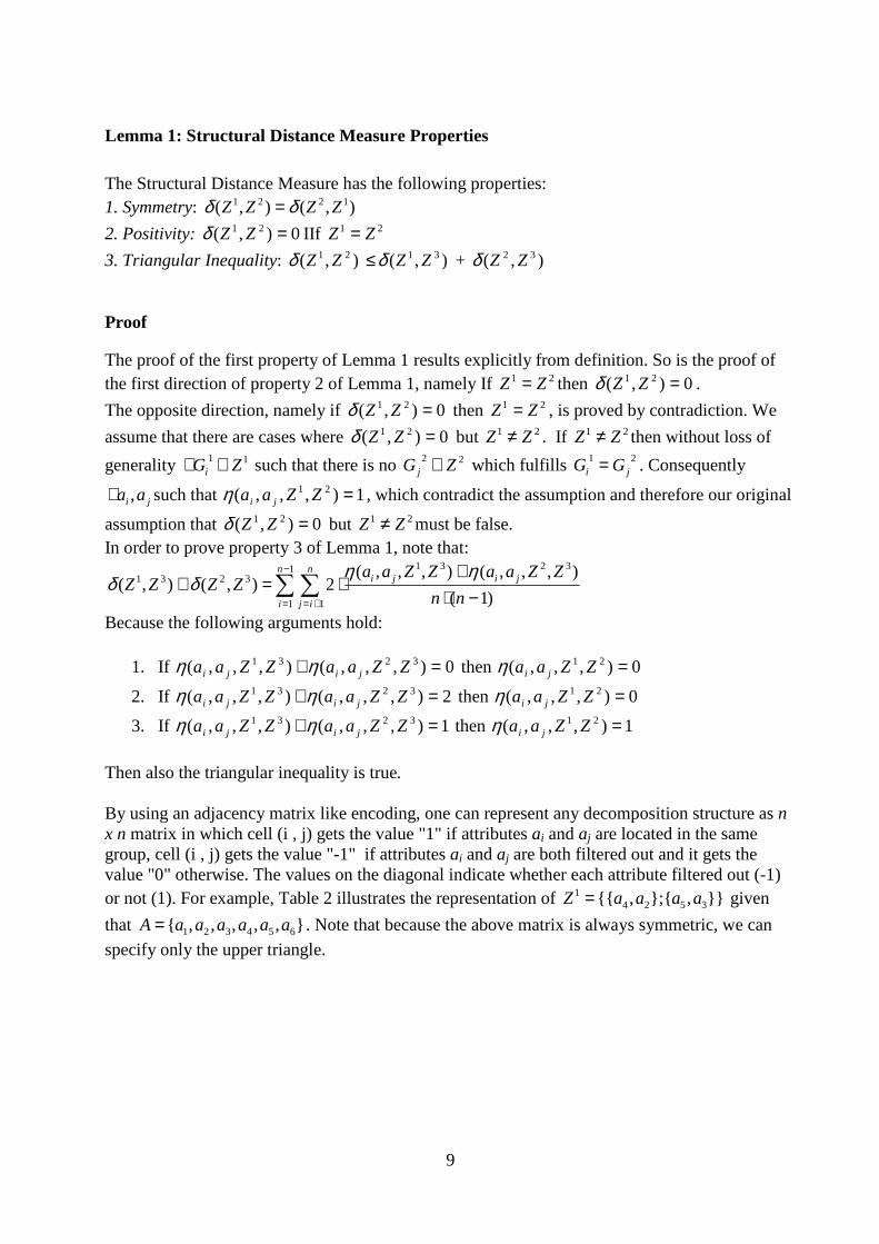
Lemma 1: Structural Distance Measure Properties

The Structural Distance Measure has the following properties: 1. Symmetry: ),(),( 1221 ZZZZ δδ =

2. Positivity: 0),( 21 =ZZδ IIf 21 ZZ =

3. Triangular Inequality: ),( 21 ZZδ ≤ ),( 31 ZZδ + ),( 32 ZZδ

Proof

The proof of the first property of Lemma 1 results explicitly from definition. So is the proof of the first direction of property 2 of Lemma 1, namely If 21 ZZ = then 0),( 21 =ZZδ .

The opposite direction, namely if 0),( 21 =ZZδ then 21 ZZ = , is proved by contradiction. We

assume that there are cases where 0),( 21 =ZZδ but 21 ZZ ≠ . If 21 ZZ ≠ then without loss of

generality 11 ZGi ∈∃ such that there is no 22 ZG j ∈ which fulfills 21ji GG = . Consequently

ji aa ,∃ such that 1),,,( 21 =ZZaa jiη , which contradict the assumption and therefore our original

assumption that 0),( 21 =ZZδ but 21 ZZ ≠ must be false. In order to prove property 3 of Lemma 1, note that:

∑ ∑−

= += −⋅+

⋅=+1

1 1

32313231

)1(

),,,(),,,(2),(),(

n

i

n

ij

jiji

nn

ZZaaZZaaZZZZ

ηηδδ

Because the following arguments hold:

1. If 0),,,(),,,( 3231 =+ ZZaaZZaa jiji ηη then 0),,,( 21 =ZZaa jiη

2. If 2),,,(),,,( 3231 =+ ZZaaZZaa jiji ηη then 0),,,( 21 =ZZaa jiη

3. If 1),,,(),,,( 3231 =+ ZZaaZZaa jiji ηη then 1),,,( 21 =ZZaa jiη

Then also the triangular inequality is true. By using an adjacency matrix like encoding, one can represent any decomposition structure as n x n matrix in which cell (i , j) gets the value "1" if attributes ai and aj are located in the same group, cell (i , j) gets the value "-1" if attributes ai and aj are both filtered out and it gets the value "0" otherwise. The values on the diagonal indicate whether each attribute filtered out (-1) or not (1). For example, Table 2 illustrates the representation of }},{};,{{ 3524

1 aaaaZ = given

that },,,,,{ 654321 aaaaaaA = . Note that because the above matrix is always symmetric, we can

specify only the upper triangle.

10

Table 2: Illustration of adjacency matrix like encoding

a1 a2 a3 a4 a5 a6 a1 -1 0 0 0 0 -1 a2 0 1 0 1 0 0 a3 0 0 1 0 1 0 a4 0 1 0 1 0 0 a5 0 0 1 0 1 0 a6 -1 0 0 0 0 -1

Definition 2: Encoding Matrix A is said to be well-defined if:

1. Commutative: ; ( , ) ( , )i j cell i j cell j i∀ ≠ = 2. Transitive: ; ( , ) 0 ( , ) 0 ( , ) 0i j k if cell i j and cell i k then cell j k∀ ≠ ≠ ≠ ≠ ≠ 3. Sign Property: ; ( , ) 0 ( , ) ( , )i j if cell i j then cell i j cell i i∀ ≠ ≠ =

We now suggest a new crossover operator call "Group-wise Crossover" (GWC) that works in the following way. We select one anchor subset from the subsets that define the first parent decomposition and one anchor subset from the subsets that define the second parent decomposition (the selected subset can be also the filtered out subset). The anchor subsets are used as-is without any addition or diminution of attributes. The first offspring is created by copying the columns and rows of the attributes that belong to the first selected anchor subset from the first parent. All remaining cells are filled in with the corresponding values that are obtained from the second parent. The second offspring is similarly created using the second anchor subset by copying the appropriate columns and the rows from the second parent and then fill in the remaining cells with the corresponding values from the first parent. Example: Assuming that two decompositions }},{};,{{ 3524

1 aaaaZ = and 2

2 6 1 4 3 5{{ , };{ , , }{ }}Z a a a a a a= are given over the feature set },,,,,{ 654321 aaaaaaA = . In order to

perform GWC operator, two anchor subsets are selected, one from every decompositions:

2 4{ , }a a from Z1 and 1 4 3{ , , }a a a from Z2. Figure 2 illustrates representations of the Z1 and Z2 and

their offspring Z3 and Z4. Z3 is obtained by keeping the group 2 4{ , }a a and the remaining cells

are copied from Z2. Z4 is obtained by keeping the group 1 4 3{ , , }a a a and the remaining cells are

copied from Z1. Thus, 32 4 1 3 5 6{{ , };{ , };{ };{ }}Z a a a a a a= and 4

1 4 3 5 2{{ , , };{ };{ }}Z a a a a a=

The highlighted cells indicate the selected group that was copied into the offspring.

11

Z1 Z2

a1 a2 a3 a4 a5 a6 a1 a2 a3 a4 a5 a6 a1 -1 0 0 0 0 -1 a1 1 0 1 1 0 0 a2 0 1 0 1 0 0 a2 0 1 0 0 0 1 a3 0 0 1 0 1 0 a3 1 0 1 1 0 0 a4 0 1 0 1 0 0 a4 1 0 1 1 0 0 a5 0 0 1 0 1 0 a5 0 0 0 0 1 0 a6 -1 0 0 0 0 -1 a6 0 1 0 0 0 1

Z3 Z4

a1 a2 a3 a4 a5 a6 a1 a2 a3 a4 a5 a6 a1 1 0 1 0 0 0 a1 1 0 1 1 0 0 a2 0 1 0 1 0 0 a2 0 1 0 0 0 0 a3 1 0 1 0 0 0 a3 1 0 1 1 0 0 a4 0 1 0 1 0 0 a4 1 0 1 1 0 0 a5 0 0 0 0 1 0 a5 0 0 0 0 1 0 a6 0 0 0 0 0 1 a6 0 0 0 0 0 -1

Figure 2: Illustration of GWC operator

Lemma 2: A projection of well-defined encoding matrix is well-defined encoding matrix.

Proof

A projection of matrix is obtained by removing certain attributes (i.e. removing their corresponding rows and columns). Without the loss of generality we assume that the removed attributes are the last t attributes. Let assume by contradiction that the projected matrix is not well-defined but the original matrix is well-defined. Because the projected matrix is not well-defined then , ,i j k n t∃ ≤ − that violates one of the constraints specified in definition 2. However because the original matrix is well-defined then for , ,i j k n∀ ≤ or more specifically for

, ,i j k n t∀ ≤ − the above constraints hold. Thus, we have reached to a contradiction and therefore our original assumption is not true.

Lemma 3: Performing GWC operator on two well-defined encoding matrices generates a

new well-defined encoding matrix

Proof

The way in which the GWC operator is defined the new offspring are obtained by diagonally concatenating the projections of the anchor subset from one parent and the remaining attributes from the second parent. Based on Lemma 2, because the parents were well-defined so are their

12

projections. It remains to show that the cells that are not obtained from the projection do nor violate definition 2. We denote by R the original attribute index of the anchor subset in the set A. Because the rows and columns of the anchor subset R are copied as-is, then cell(i,j)= cell(j,i)=0 for ;i R j R∀ ∈ ∉ . Therefore constrain 1 in definition 2 is always true and constraints 2 and 3 are not relevant in this case. Lemma 4: Operator GWC creates offspring that their distance is not greater than the distance of their parents.

Proof

We denote by Z1 and Z2 the parent solutions and by Z3 and Z4 the offspring. Because each cell of the offspring are obtained from one of the parent then,

3 1 3 2 1 2( , ) ( , ) ( , )Z Z Z Z Z Zδ δ δ+ = 4 1 4 2 1 2( , ) ( , ) ( , )Z Z Z Z Z Zδ δ δ+ =

The last equation is true because in Equation (4), the term 1 2( , , , ) 0i ja a Z Zη = if cells (i,j) in

both matrices are equal. Using the triangular inequality we obtain that:

3 4 3 1 4 1( , ) ( , ) ( , )Z Z Z Z Z Zδ δ δ≤ + 3 4 3 2 4 2( , ) ( , ) ( , )Z Z Z Z Z Zδ δ δ≤ +

Thus:

3 4 3 1 4 1 3 2 4 22 ( , ) ( , ) ( , ) ( , ) ( , )Z Z Z Z Z Z Z Z Z Zδ δ δ δ δ≤ + + + or:

3 3 1 2( , ) ( , )Z Z Z Zδ δ≤ Lemma 4 indicates that the GWC operator together with the proposed encoding does not slow down the convergence of the genetic algorithm. Together with the selection process that prefers solutions with higher fitness values, one can ensure that the algorithm does converge (Louis and Rawlins, 1993). As to the mutation operator, according to a certain probability (Pmut) each attribute can be cut off from its original group and join another randomly selected group.

13

3.3 Fitness Function In each iteration, we have to create a new population from the current generation. The selection operation determines which parent chromosomes participate in producing offspring for the next generation. Usually, members are selected for mating with a selection probability proportional to their fitness values. The most common way to implement this method is to set the selection probability pi equal to:

ii

jj

fpf

=∑

(6)

For a classification problem, the fitness value fi of the ith member can the complement to 1 of the generalization error. Note that using training error as-is is not sufficient for evaluating classifiers due to over-fitting phenomena. The following subsections present two evaluation methods for the generalization error. The first method utilizes the Wrapper methodology. The second method uses a new VC-Dimension bound developed for this purpose. 3.3.1 Wrapper Approach The most straightforward to estimate generalization error is to use the wrapper procedure. In this approach the decomposition structure is evaluated by repeatedly sampling the training set and measuring the accuracy of the inducers obtained for this decomposition on an unused portion of the training set. This is the most common approach for evaluate the fitness function in attribute selections problems. 3.3.2 VC-Dimension Framework An alternative approach for evaluating performance is to use the generalization error bound in terms of the training error and concept size. In the book “Mathematics of Generalization”, Wolpert (1995) discuss four theoretical frameworks for estimating the generalization error, namely: PAC, VC and Bayesian, and Statistical Physics. All these frameworks combine the training error (which can be easily calculated) with some penalty function expressing the capacity of the inducers. In this paper we decided to use the VC theory for evaluating the generalization error bound. According to the VC theory the bound on the generalization error of hypothesis space H with finite VC-Dimension d is given by:

md

md

ShDh 4ln)1

2(ln

),(ˆ),(

δ

εε−+⋅

≤− 0>∀

∈∀δ

Hh

(7)

14

with probability of 1 δ− . where ˆ( , )h Sε represents the training error of classifier h measured on training set S of cardinality m and ( , )h Dε represents the generalization error of the classifier h over the distribution D. In order to use the bound (Equation 7), one needs to measure the VC-Dimension. The VC dimension for a set of indicator functions is defined as the maximum number of data points that can be shattered by the set of admissible functions. By definition, a set of m points is shattered by a concept class if there are concepts (functions) in the class that split the points into two classes in all of the 2m possible ways. The VC dimension might be difficult to compute accurately and it depends on the induction algorithm.

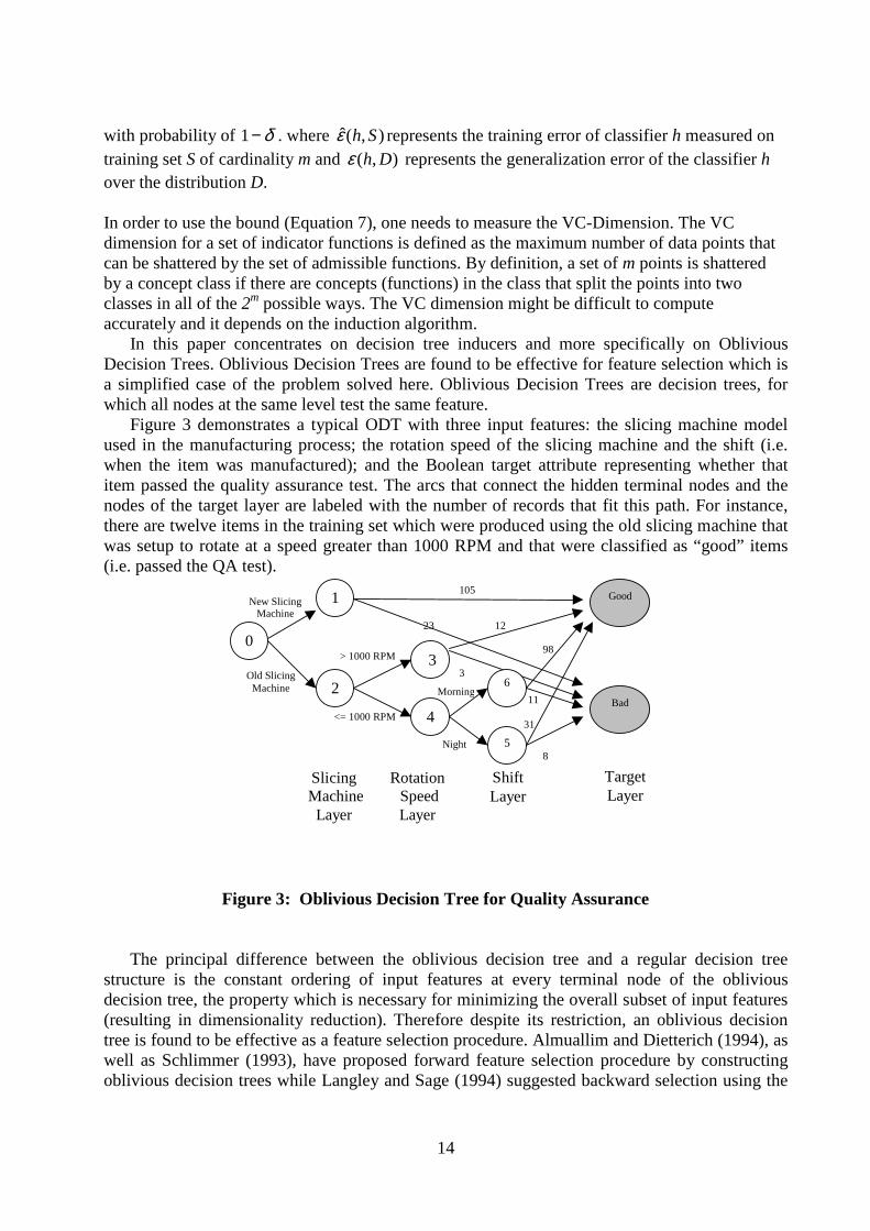
In this paper concentrates on decision tree inducers and more specifically on Oblivious Decision Trees. Oblivious Decision Trees are found to be effective for feature selection which is a simplified case of the problem solved here. Oblivious Decision Trees are decision trees, for which all nodes at the same level test the same feature.

Figure 3 demonstrates a typical ODT with three input features: the slicing machine model used in the manufacturing process; the rotation speed of the slicing machine and the shift (i.e. when the item was manufactured); and the Boolean target attribute representing whether that item passed the quality assurance test. The arcs that connect the hidden terminal nodes and the nodes of the target layer are labeled with the number of records that fit this path. For instance, there are twelve items in the training set which were produced using the old slicing machine that was setup to rotate at a speed greater than 1000 RPM and that were classified as “good” items (i.e. passed the QA test).

0

Bad

1

2

3

4

6

5

Good New Slicing Machine

Slicing Machine

Layer

Old Slicing Machine

Shift Layer

Night

Morning

Rotation Speed Layer

<= 1000 RPM

> 1000 RPM

Target Layer

105

23 12

3

8

31

98

11

Figure 3: Oblivious Decision Tree for Quality Assurance

The principal difference between the oblivious decision tree and a regular decision tree

structure is the constant ordering of input features at every terminal node of the oblivious decision tree, the property which is necessary for minimizing the overall subset of input features (resulting in dimensionality reduction). Therefore despite its restriction, an oblivious decision tree is found to be effective as a feature selection procedure. Almuallim and Dietterich (1994), as well as Schlimmer (1993), have proposed forward feature selection procedure by constructing oblivious decision trees while Langley and Sage (1994) suggested backward selection using the

15

same means. Recently Last et al. (2002) have suggested a new algorithm for constructing oblivious decision trees, called IFN (Info-Fuzzy Network) which is based on information theory.

In the case of feature set decomposition each subset is represented by an oblivious decision tree and each feature is located on a different layer. As a result, adding a new feature to a subset is performed by adding a new layer and connecting it to the nodes of the last layer. The nodes of a new layer are defined as the Cartesian product combinations of the previous layer’s nodes with the values of the new added feature. In order to avoid unnecessary splitting, the algorithm splits a node only if it is useful. In this paper we split a node, if the information gain of the new feature in this node is strictly positive.

The unique structure of oblivious decision tree is very convenient to our genetic algorithm approach. Moving from one generation to the other usually require a small changes on the subset structures. Because each feature is located on a different layer, it relatively easy to add or remove features incrementally; As opposed to regular decision tree inducers in which each iteration of the search may require generating the decision tree from scratch. As stated before, using an oblivious decision tree may be attractive in this case as it adds features to a classifier in an incremental manner. Oblivious decision trees can be considered as restricted decision trees. For that reason any generalization error bound that has been developed for decision trees in the literature (Mansour and McAllester, 2000) can be used in this case also. However, there are several reasons to develop a specific bound. First, by utilizing the fact that the oblivious structure is more restricted, it might be possible to develop a tighter bound. Second, in this case it is required to extend the bound for several oblivious trees combined using the Naive Bayes combination. The following theorem introduces an upper bound and a lower bound of the VC dimension that was recently proposed by us in the hill-climbing algorithm for feature set decomposition (Rokach and Maimon, 2005). The hypothesis class of multiple mutually exclusive oblivious decision trees

can be characterized by two vectors and one scalar: 1( ,..., )L l lω=�

, 1( ,..., )T t tω=�

and n, where lk

is the numbers of layers (not including the root and target layers) in the tree k, tk is the number of terminal nodes in the tree k and n is the number of input features. For the sake of simplicity, the bound described in this section is developed assuming that the input features and the target feature are both binary. This bound can be extended for other cases in a straightforward manner. Note that each oblivious decision tree with non-binary input features can be converted to a corresponding binary oblivious decision tree by using appropriate artificial features. Theorem 1: Upper and Lower Bound for VC dimension of Multiple Oblivious Decision Trees Combined with Naive Bayes The VC-Dimension of ω mutually exclusive oblivious decision trees on n binary input features

that are combined using the Naive Bayes combination and that have 1( ,..., )L l lω=�

layers and

1( ,..., )T t tω=�

terminal nodes is not greater than: log 1

2( 1) log(2 ) 2 log 1

F U

F e U

ωω

+ = + + >

and at least: 1F ω− +

16

where:1

ii

F tω

=

=∑ 1

1

(2 4)!!

( 2)! ( 2)!! ( )!

i

i i ii

i

tnU

t tn l

ω

ω

ω =

=

−= ⋅

− ⋅ −⋅ −∏

∑.

The proof of the Theorem can be found in (Rokach and Maimon, 2005). 3.4 Caching Mechanism The Achilles heel of using genetic algorithm in feature set decomposition problem is that it requires the creation of a classifier for each subset in each solution candidate. Assuming that there are G generations, the population size is L, and that each solution has on average D subsets, then :G L D⋅ ⋅ classifiers are created. Recall that by using oblivious decision trees we might not need to create from scratch each classifier but reuse classifiers that have already created. It is well know fact that one can trade computational complexity with storage complexity. Thus we suggest using the following caching mechanism. First of all when moving from one generation to the consequent generation, we can use all subsets that have remained without any change. By using the GWC operator and ignoring the mutation, each member in the new population has at least one subset (the anchor subset) that has not been changed at all. Moreover all other subsets have some common members. In that case we can not use the oblivious decision tree as-is because the original tree might use attributes that are not used in the inherited subset. For this purpose we eliminate attributes from the oblivious tree, layer by layer until we obtain an oblivious decision tree that all its attributes are used in the inherited subset. Example: Assuming that two decompositions 1

2 4 5 3{{ , };{ , }}Z a a a a= and 2

2 6 1 4 3 5{{ , };{ , , }{ }}Z a a a a a a= are given over the feature set },,,,,{ 654321 aaaaaaA = . We also

assume that in the previous generation the following attribute order has been used in the created oblivious decision trees: 4 2 5 3;a a a a→ → 2 6 1 3 4 5; ; ;a a a a a a→ → →

Recall that by using the GWC operator (and ignoring the mutation operator), the following subsets may be obtained: 3

2 4 1 3 5 6{{ , };{ , };{ };{ }}Z a a a a a a= and 41 4 3 5 2{{ , , };{ };{ }}Z a a a a a= .

Thus in order to create the oblivious decision trees to Z3 and Z4, we can use the following oblivious decision trees as-is: 4 2;a a→ 1 3 4 5;a a a a→ → . The oblivious tree for 6{ }a will be

created from scratch. The remaining subsets can be (partially or completely) obtained by removing attributes from the existing oblivious decision trees. The tree for1 3{ , }a a can be

obtained by removing attribute 6a from 2 6a a→ . This removal is possible as 4a is located last.

The tree for 2{ }a can be obtained by removing attribute 4a from 1 3 4a a a→ → .

Additionally to using the oblivious decision trees of the previous generations, we can use the existing resemble in different subset of the current generation. While generating a decision tree, we check at the end of each iteration (i.e. after adding a new attribute to the decision tree) if there is another solution in the current generation that also group these features together in the same subset. If this is the case, we store the current decision tree in the memory cache for future use. Later on when time has come to generate the decision tree for the solution with the common

17

subset, instead of creating the tree from scratch we use the tree that was stored in the caching mechanism. For example if in the first generation we have the following members:

1 1 4 5 6 2 3 8 10 7 9{ , , , }; { ; ; ; }; { ; }Z a a a a a a a a a a=

2 1 5 6 8 2 3 4 10 7 9{ , , , }; { ; ; ; }; { ; }Z a a a a a a a a a a=

3 1 3 4 5 6 2 8 10 7 9{ , , , , }; { ; ; }; { ; }Z a a a a a a a a a a=

Assuming that we are evaluating the members one by one according to the above order and that while creating the tree for the first subset in the first solution we got a decision tree with the following order 5 1 6 a a a→ → then we might want to store this tree in the caching

mechanism, and use it also in members 2 and 3. It should be noted that using this caching mechanism reduce the search space, because it dictates the order in which the features are located in the decision tree. For instance in the last example the first tree of solution 2 could have the following structure: 8 1 5 6a a a a→ → → . However by

using the tree 5 1 6 a a a→ → that was stored in the cache we ignore this structure in advance. In

order to solve this dilemma we decided no to store small trees (in this paper less than 3 attributes). In these cases the saving in computational complexity is not worth the loss in generalization capability. Obviously we would like to store in the cache the longest common subset. Thus in each iteration we check if the current tree still can be used by the same number of solutions. If this is the case the current tree will replace the older one.

4. Experimental Study 4.1 Overview The aim of this experimental study is to examine whether the genetic algorithm framework for feature set decomposition approach can improve the classification performance in mining quality assurance problems. For this purpose, a comparative experiment was conducted on three real-life datasets obtained from two manufacturers with an average yearly income of more than 1 billion dollars. The first dataset was obtained from a manufacturer of dairy products. The last two datasets were obtained from a wafer manufacturer.

This study examines an implementation of genetic algorithm to feature set decomposition using the suggested adjacency matrix encoding, GWC operator and fitness function that is based on the VC dimension of multiple oblivious decision trees combined with Naive Bayes. This algorithm is called GOV (Genetic algorithm for Oblivious decision tree using VC-dimension estimation). The performance of GOV algorithm is compared with our previous feature set decomposition (BOW), Naive Bayes and C4.5 (Quinlan, 1993) algorithms. The Naïve Bayes was chosen since it represents a specific point in the search space of the GOV algorithm. The C4.5 algorithm was selected because it is considered as a state-of-the-art decision tree algorithm which is widely

18

used in many other comparative studies. The following subsections describe each one of the case studies and the results. 4.2 Manufacturing Cottage Cheese 4.2.1 Objective Manufacturing cottage cheese is one of the most complicated processes in producing dairy products. The process, which may take up to 20 hours, usually involves many stages. During this long process, a few hundred parameters can be measured or adjusted. As in every dairy product, there is a chance that a specific batch will be found sour when consumed by the customer, prior to the end of the product’s shelf-life. During its shelf-life, the product’s pH value normally drops. When it reaches a certain value, the consumer reacts to it as a spoiled product; even though there is no any bacteriological problem. For every batch manufactured, the dairy department performs randomly tests for pH as well organoleptic (taste) at the end of the shelf-life. The samples are kept in the laboratory at a temperature of 7ºC, compared to 4ºC, which is the recommended storage temperature in a home refrigerator. The higher laboratory temperature simulates abuse handling of the product along the cooling chain. The product shelf-life is determined by the dairy department (generally 12-14 days), assuming that the product retains its organoleptic properties to the end of its shelf-life.

The aim of this experiment was to identify batches with a high probability of becoming sour (at the end of shelf-life) based on the process variables. For this purpose we built a classification model that is capable to classify each batch into its anticipated quality level. By having the ability to identify in advance manufacturing patterns with impact on the quality, the manager can replace low quality anticipated manufacturing setting with a better setting. 4.2.2 Data The training data set includes 800 records. Each record has 70 input attributes representing various manufacturing variables. Most of the parameters fall into one of the following classes: temperature, duration, raw material quantities and machines. For example we have used the following attributes: average cooling temperature, scalding duration, calcium quantity, culture quantity, etc. The target attribute represents the pH value after two weeks. It can have two values: "Tasty" (pH 4.9-5.3) and "Sour" (below pH 4.9). 4.2.3 Results In order to compare the results of GOV to other algorithms, we used the 10-fold cross-validation procedure. According to this procedure, the training set was randomly partitioned into 10 disjoint instance groups. Each instance group was used once in a test set and nine times in a training set. Since the accuracy on the validation instances is a random variable, the confidence interval was estimated by using the normal approximation. Table 3 shows the overall accuracy obtained by using 10-fold cross-validation along with their confidence interval. A paired two-sample student's t-test has been performed in order to determine whether a sample's means are distinct. The superscript "+" indicates that the accuracy rate of GOV was significantly higher than the corresponding algorithm at confidence level of 5%. It should be noted that both feature set decomposition methods have improved accuracy.

19

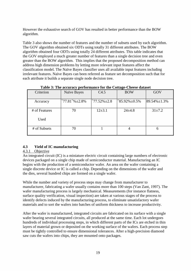
However the exhaustive search of GOV has resulted in better performance than the BOW algorithm. Table 3 also shows the number of features and the number of subsets used by each algorithm. The GOV algorithm obtained six ODTs using totally 31 different attributes. The BOW algorithm obtained four ODTs using totally 24 different attributes. This table indicates that the GOV employed a much greater number of features than a single decision tree and even greater than the BOW algorithm. This implies that the proposed decomposition method can address high dimension problems by letting more relevant input features affect the classification model. The Naïve Bayes classifier uses all available input features including irrelevant features. Naïve Bayes can been referred as feature set decomposition such that for each attribute it builds a separate single node decision tree.

Table 3: The accuracy performance for the Cottage-Cheese dataset Criterion Naïve Bayes C4.5 BOW GOV

Accuracy +77.81+%±2.8% +77.52%±2.8 +85.92%±0.5% 89.54%±1.3%

# of Features

Used

70 12±3.1 24±4.8 31±7.2

# of Subsets 70 1 4 6

4.3 Yield of IC manufacturing 4.3.1 Objective An integrated circuit (IC) is a miniature electric circuit containing large numbers of electronic devices packaged on a single chip made of semiconductor material. Manufacturing an IC begins with the production of a semiconductor wafer. An area on the wafer containing a single discrete device or IC is called a chip. Depending on the dimensions of the wafer and the dies, several hundred chips are formed on a single wafer. While the number and variety of process steps may change from manufacturer to manufacturer, fabricating a wafer usually contains more than 100 steps (Van Zant, 1997). The wafer manufacturing process is largely mechanical. Measurements (for instance flatness, surface quality verification, visual inspection) are taken at various stages of the process to identify defects induced by the manufacturing process, to eliminate unsatisfactory wafer materials and to sort the wafers into batches of uniform thickness to increase productivity. After the wafer is manufactured, integrated circuits are fabricated on its surface with a single wafer bearing several integrated circuits, all produced at the same time. Each lot undergoes hundreds of individual processing steps, in which different parts of the ICs are etched in thin layers of material grown or deposited on the working surface of the wafers. Each process step must be tightly controlled to ensure dimensional tolerances. After a high-precision diamond saw cuts the wafers into chips, they are mounted onto packages.

20

Fabrication of a single lot requires several months. The data are accumulated for each fabrication tool at both the wafer and lot level, using an information system known as “manufacturing execution system”. IC manufacturing lines provide many data-mining opportunities. In IC manufacturing, data-mining could have tremendous economic impact, raising profitability by increasing throughput and reducing costs, consequently (Fountain et al., 2000). For this paper we examined two different datasets obtained from a wafer manufacturer providing design support, manufacturing and turnkey services for integrated ICs on silicon wafers in geometries from 1.0 to 0.18 microns. The main goal of data mining in IC manufacturing databases is to understand how different parameters in the process affect the line throughput. The throughput of IC manufacturing processes is measured by “yield,” which is the number of good products (chips) obtained from a silicon wafer. Since the capability of very expensive microelectronics equipment usually limits the number of wafers processed per time unit , the yield is the most important criterion in determining the effectiveness of an IC process. 4.3.2 Data The training dataset includes only 70 records. Each record represents a single wafer and has 257 input attributes labelled p1,…,p257 that represent the setting of various parameters used in the manufacturing process of this wafer. The target attribute represents the yield, which the manufacturer's quality engineer has manually divided into two groups: High and Low. More than half of the attributes are numeric. The input attributes specify several machine parameters (for instance, the rotation speed of the slicing machine or the slicing machine model ) that may affect the yield. A distinctive value (in case of categorical attributes) or the mean value (in case of numeric values) replace missing values. Due to the high commercial confidentiality of the process data, we will not explain here the specific meaning of the measured parameters. 4.3.3 Results Table 4 presents the overall accuracy. The results indicate that both BOW and GOV achieved better results in accuracy compared to the C4.5 and Naïve Bayes. GOV has slightly better results. However as opposed to the first case study the difference between GOV and BOW mean accuracy is not statistically significant. Moreover, as in the first case study, the BOW and GOV algorithms employed a greater number of features than C4.5.

Table 4: The accuracy for the yield dataset

Criterion Naïve Bayes C4.5 BOW GOV

Accuracy +84.28%±2.1% +78.85%±3.6% 92.86%5.3% 93.17%4.6%

# of Features Used 257 4±1.4 16±7.9 22±7.2

# of Subsets 70 1 5 5

21

4.4 The IC test 4.4.1 Objectives The fabricated ICs undergo two series of exhaustive electric tests that measure the operational quality. The first series of tests, which is used for reducing costs by avoiding packaging defective chips, is performed while ICs are still in wafer form. The second series of tests, which is used for quality assurance of the final chip, is carried out immediately after the wafers are cut into chips and mounted onto packages. The electric tests are performed by feeding various combinations of input signals into the IC. The output signal is measured in each case and compared to the expected behaviour. There are wafers that perform well on the first series but fail later in the second series. The goal is to check whether the results of the first series can be further analyzed in order to predict the outcome of the second series. This can be used to reduce the number of wafers that are unnecessarily sliced and packed, eliminating the need for a second series of exhaustive electric tests for most of the devices. 4.4.2 Data The training data set includes 395 records. Each record has 220 input attributes labeled p1,…,p220 representing the electric result values obtained in the first series of tests. Most of the input features represent voltage levels. The target attribute is binary representing "pass" and "not pass" devices according to the functionality of the device in the second testing series. Similar to the yield problem, a distinctive value or the average value replaces missing values depending on the data type. 4.4.3 Results Running the GOV algorithm on the above data has created 9 ODTs containing 34 electronic tests that can be used as indicators for the results of the second series of tests. Table 5 shows the mean accuracy obtained by using 10-fold cross-validation along with their confidence interval (with a confidence level of 95%). As in the case of the yield dataset, the GOV algorithm obtained the most encouraging results.

Table 5: The accuracy for the IC-Test dataset Criterion Naïve Bayes C4.5 BOW GOV

Accuracy +92.82%±2.5% +89.24%±1.9% 96.81%±0.6% 97.17%1.3%

# of Features Used 220 9±3.2 26±2.7 34±3.1

# of Subsets 220 1 7 9

5. Conclusion Classification problems in quality assurance are characterized by many contributing features relative to the training set size. This paper presents a new, mutually exclusive feature set

22

decomposition methodology designed specifically for these circumstances. The basic idea is to decompose the original set of features into several subsets, build a decision tree for each projection, and then combine them. This paper examine if genetic algorithm can be useful for discovering the appropriate decomposition structure. For this purpose we have suggested a new encoding schema and fitness function that was specially designed for feature set decomposition with oblivious decision trees. Additionally a caching mechanism has been implemented in order to reduce computational complexity. The proposed framework was tested with over three real-life datasets. The results show that this framework tends to outperform other comparable methods in the accuracy. The above leads to the conclusion that feature set decomposition can be used for solving classification problems in quality assurance and that using genetic algorithm can lead better results than hill-climbing methods. Additional issues to be further studied include: examining how the feature set decomposition concept can be implemented using other inducers like neural networks and by examining other techniques to combine the generated classifiers (like voting).

References

1. Almuallim, H. and Dietterich, T.G. (1994) 'Learning Boolean concepts in the presence of many irrelevant features'. Artificial Intelligence, 69: 1-2, 279-306.

2. Domingos, P. and Pazzani, M. (1997) 'On the Optimality of the Naive Bayes Classifier under Zero-One Loss', Machine Learning, 29: 2, 103-130.

3. Fountain, T. Dietterich T. and Sudyka B. (2000) 'Mining IC Test Data to Optimize VLSI Testing'', Proc. 6th ACM SIGKDD Conference, Simoff J., Zaiane O., eds., Boston, MA, USA, pp. 18-25.

4. Freitas, A. (2005) 'Evolutionary Algorithms for Data Mining', The Data Mining and Knowledge Discovery Handbook, Maimon O. and Rokach L., eds., Springer, pp. 435-467.

5. Gardner, M. and Bieker, J. (2000) 'Data mining solves tough semiconductor manufacturing problems'. Proc. 6th ACM SIGKDD Conference, Simoff J., Zaiane O., eds., Boston, MA, USA, pp. 376-383.

6. Goldberg, D. (1989) 'Genetic Algorithms in Search, Optimization, and Machine Learning. Reading', MA: Addison-Wesley.

7. Hsu, W.H., Welge M., Wu J. and Yang T. (1999) 'Genetic algorithms for selection and partitioning of attributes in large-scale data mining problems', Proc. of the Joint AAAI-GECCO Workshop on Data Mining with Evolutionary Algorithms, Freitas A., edt. Orlando, FL, July, pp. 1-6.

8. Hsu, W. H. (2004) 'Genetic wrappers for feature selection in decision tree induction and variable ordering in Bayesian network structure learning', Information Sciences, 163(1-3):103-122.

9. Kudo, M. and Sklansky J. (2000) 'Comparison of algorithms that select features for pattern classifiers', Pattern Recognition, 33: 25-41.

10. Kusiak, A. (2000) 'Decomposition in Data Mining: An Industrial Case Study', IEEE Transactions on Electronics Packaging Manufacturing, 23(4) pp. 345-353.

23

11. Kusiak, A. (2001) 'Rough Set Theory: A Data Mining Tool for Semiconductor Manufacturing', IEEE Transactions on Electronics Packaging Manufacturing, 24(1) pp. 44-50.

12. Kusiak, A. and Kurasek, C. (2001) 'Data Mining of Printed-Circuit Board Defects', IEEE Transactions on Robotics and Automation, 17(2) pp. 191-196.

13. Langley, P. and Sage, S. (1994) 'Induction of selective Bayesian classifiers', Proc. of the Tenth Conference on Uncertainty in Artificial Intelligence, Seattle, WA: Morgan Kaufmann, pp. 399-406.

14. Last, M. and Kandel, A. (2001) 'Data Mining for Process and Quality Control in the Semiconductor Industry', Data Mining for Design and Manufacturing: Methods and Applications, Braha D., ed., Kluwer Academic Publishers, pp. 207-234.

15. Louis, S. J. and Rawlins G. J. E. (1993), 'Predicting convergence time for genetic algorithms', Foundations of Genetic Algorithms 2, Whitley L. D., editor, Morgan Kaufmann, pp. 141-161.

16. Maimon, O., and Rokach, L. (2001) 'Data Mining by Attribute Decomposition with semiconductors manufacturing case study', Data Mining for Design and Manufacturing: Methods and Applications, Braha D. ed., Kluwer Academic Publishers, pp. 311-336.

17. Mansour, Y. and McAllester, D. (2000). Generalization Bounds for Decision Trees, Proc. of the 13th Annual Conference on Computer Learning Theory, San Francisco, Morgan Kaufmann, pp. 69-80.

18. Opitz, D., and Shavlik, J. (1996) 'Actively searching for an effective neural-network ensemble'. Connection Science, 8(3/4):337-353.

19. Opitz, D. (1999), 'Feature Selection for Ensembles', Proc. 16th National Conf. on Artificial Intelligence, Orlando, Florida , pp. 379-384.

20. Quinlan, J. R. (1993) 'C4.5: Programs for Machine Learning', Morgan Kaufmann 21. Rokach, L. and Maimon O., 'Feature Set Decomposition for Decision Trees', Journal of

Intelligent Data Analysis, 9(2):131-158. 22. Rokach, L. and Maimon O. (2006) 'Data mining for improving the quality of

manufacturing: a feature set decomposition approach', Journal of Intelligent Manufacturing (Accepted for publication).

23. Schlimmer, J. C. (1993) 'Efficiently inducing determinations: A complete and systematic search algorithm that uses optimal pruning'. Proc. of the International Conference on Machine Learning, San Mateo, CA, Morgan Kaufmann, pp 284-290.

24. Sharkey, A. (1996) 'On combining artificial neural nets', Connection Science, 8: 299-313. 25. Sharpe, P.K. and Glover, R.P. (1999) 'Efficient GA based techniques for classification',

Applied Intelligence, 11: 277-284,. 26. Van Zant, P. (1997) 'Microchip Fabrication: a Practical Guide to Semiconductor

Processing', New York: McGraw-Hill. 27. Wolpert, D. H. (1995) 'The relationship between PAC, the statistical physics framework,

the Bayesian framework, and the VC framework', The Mathematics of Generalization, Wolpert D. H. ed., The SFI Studies in the Sciences of Complexity, Addison-Wesley, pp. 117-214.