Mining Association Rules Mining Association Rules of Simple Conjunctive of Simple Conjunctive QueriesQueries

Bart Goethals

Wim Le Page

Heikki Mannila

SIAM 08

112/04/19 1

Outline.Outline.MotivationPreliminariesConqueror : algorithm

◦Selection loop◦Projection loop◦Constants loop◦Eliminating redundancies

ExperimentsConclusion

112/04/19 2

Motivation.Motivation.First query ask for the actors have

starred in a movie of the genre ‘drama’.

Second query ask for ‘drama’ and ‘comedy’.

Now suppose the answer to the first query consists of 1000 actors, and the answer to the second query consists of 900 actors.

112/04/19 3

MotivationMotivation(cont)(cont)

It reveals the potentially interesting pattern that actors starring in ‘drama’ movies typically (with a probability of 90%) also star in a ‘comedy’ movie.

In general, we are looking for pairs of queries Q1,Q2, such that Q1 asks for a set of tuples satisfying a certain condition and Q2 asks for those tuples satisfying a more specific condition.

112/04/19 4

Preliminaries.Preliminaries.Relational database: R(R1,…,Rn)

Definition 1: ◦Simple Conjunctive Query πXσF (R1 ×···× Rn)

◦F : Ri.A = Rj.B or Rk.A=“c”

◦x : attributes from R

example : Q1: πA,BR or Q2 : πA,B σA=B R

112/04/19 5

PreliminariesPreliminaries(cont)(cont)

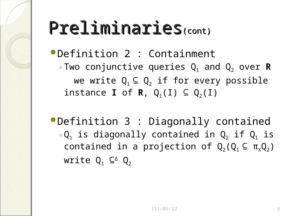
Definition 2 : Containment◦Two conjunctive queries Q1 and Q2 over R

we write Q1 ⊆ Q2 if for every possible instance I of R, Q1(I) ⊆ Q2(I)

Definition 3 : Diagonally contained◦Q1 is diagonally contained in Q2 if Q1 is

contained in a projection of Q2(Q1 ⊆ πXQ2)

write Q1 ⊆Δ Q2

112/04/19 6

PreliminariesPreliminaries(cont)(cont)

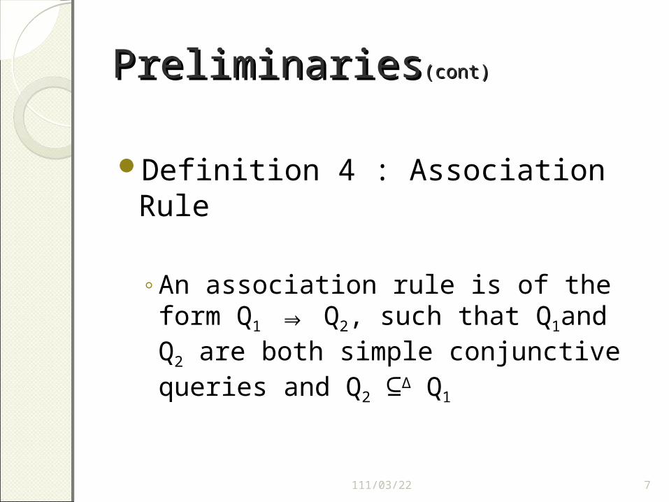
Definition 4 : Association Rule

◦An association rule is of the form Q1 ⇒ Q2, such that Q1and Q2 are both simple conjunctive queries and Q2 ⊆Δ Q1

112/04/19 7

PreliminariesPreliminaries(cont)(cont)

Definition 5 : Support

◦The support of a conjunctive query Q in an instance I is the number of distinct tuples in the answer of Q on I.

◦A query is said to be frequent in I if its support exceeds a given minimal support threshold.

◦The support of an association rule Q1 ⇒ Q2 in I is the support of Q2 in I, an association rule is called frequent in I if Q2 is frequent in I.

112/04/19 8

PreliminariesPreliminaries(cont)(cont)

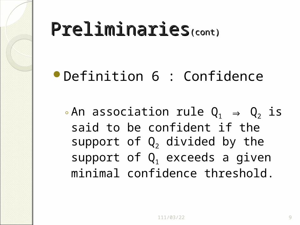
Definition 6 : Confidence

◦An association rule Q1 ⇒ Q2 is said to be confident if the support of Q2 divided by the support of Q1 exceeds a given minimal confidence threshold.

112/04/19 9

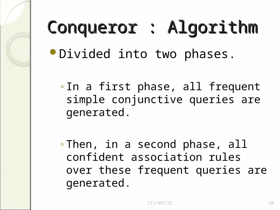
Conqueror : AlgorithmConqueror : AlgorithmDivided into two phases.

◦In a first phase, all frequent simple conjunctive queries are generated.

◦Then, in a second phase, all confident association rules over these frequent queries are generated.

112/04/19 10

AlgorithmAlgorithm(cont)(cont)

Property 1 : ◦Let Q1 and Q2 be two simple

conjunctive queries. If Q2 ⊆Δ Q1, then support(Q1) ≥ support(Q2).

112/04/19 11

AlgorithmAlgorithm(cont)(cont)

Selection loop: ◦ Generate all instantiations of F, without

constants, in a breadth-first manner.

Projection loop: ◦ For each generated selection, generate all

instantiations of X in a breadth-first manner, and test their frequency.

Constants loop: ◦ For each generated query in the projection

loop, add constant assignments to F in a breadth-first manner.

112/04/19 12

AlgorithmAlgorithm(cont)(cont)

Selection loop◦We will use the so called restricted

growth string for generating all partitions.

◦A Restricted Growth string is an array a[1 ...m] where m is the total number of attributes occurring in the database.

◦Restricted growth string satisfies the following growth inequality (for i =1, 2,...,n − 1, and with a[1] = 1):

a[i +1] ≤ 1+max a[1],a[2],...,a[i].

112/04/19 13

AlgorithmAlgorithm(cont)(cont)

a[1] = 1i=1, a[1+1] ≤ 1 + max{a[1]} = 2i=2, a[2+1] ≤ 1 + max{a[1], a[2]} = 3

.

.

.

EXAMPLE 4. ◦Let A1,A2,A3,A4 be the set of all attributes

occurring in the database. Then, the restricted growth string 1221 represents the conjunction of equalities A1 = A4, A2 = A3.

112/04/19 14

AlgorithmAlgorithm(cont)(cont)

112/04/19 15

AlgorithmAlgorithm(cont)(cont)

Before generating possible projections for a given selection, we first determine whether the selection represents a cartesian product.

112/04/19 16

AlgorithmAlgorithm(cont)(cont)

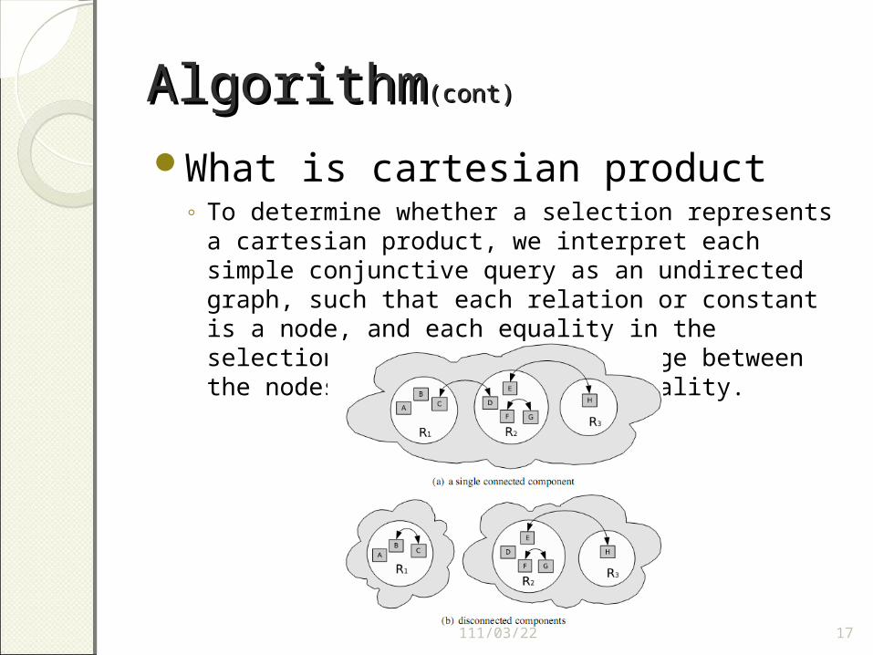
What is cartesian product◦ To determine whether a selection represents a

cartesian product, we interpret each simple conjunctive query as an undirected graph, such that each relation or constant is a node, and each equality in the selection of the query is an edge between the nodes occurring in that equality.

112/04/19 17

AlgorithmAlgorithm(cont)(cont)

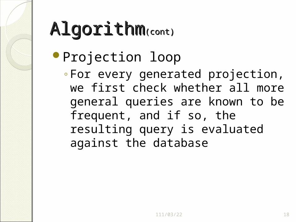
Projection loop◦For every generated projection, we

first check whether all more general queries are known to be frequent, and if so, the resulting query is evaluated against the database

112/04/19 18

AlgorithmAlgorithm(cont)(cont)

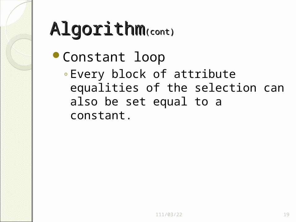
Constant loop◦Every block of attribute equalities of

the selection can also be set equal to a constant.

112/04/19 19

AlgorithmAlgorithm(cont)(cont)

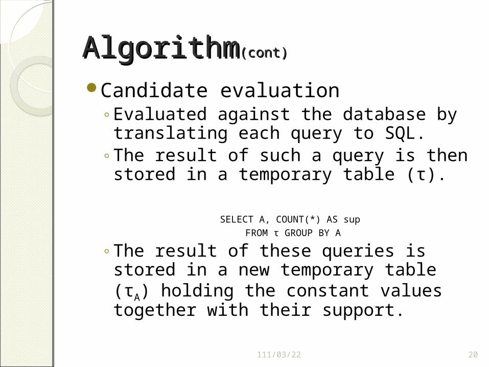
Candidate evaluation◦Evaluated against the database by

translating each query to SQL.◦The result of such a query is then

stored in a temporary table (τ).

SELECT A, COUNT(*) AS sup FROM τ GROUP BY A

◦The result of these queries is stored in a new temporary table (τA) holding the constant values together with their support.

112/04/19 20

AlgorithmAlgorithm(cont)(cont)

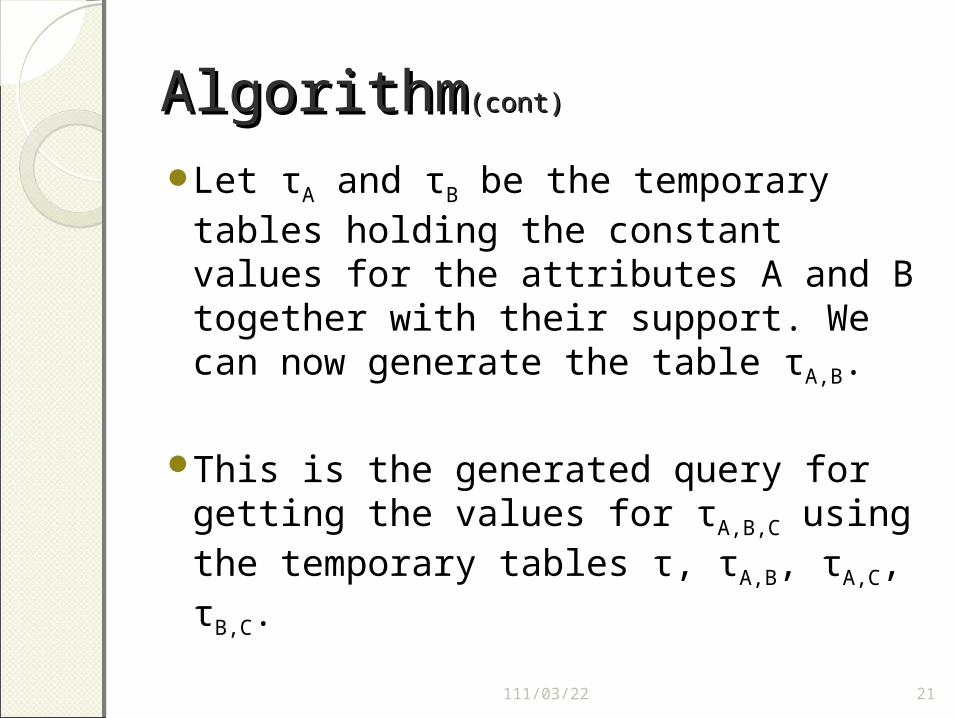
Let τA and τB be the temporary tables holding the constant values for the attributes A and B together with their support. We can now generate the table τA,B.

This is the generated query for getting the values for τA,B,C using the temporary tables τ, τA,B, τA,C, τB,C.

112/04/19 21

AlgorithmAlgorithm(cont)(cont)

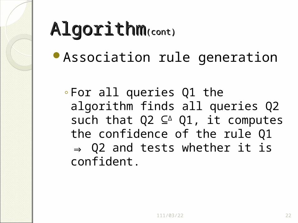
Association rule generation

◦For all queries Q1 the algorithm finds all queries Q2 such that Q2 ⊆Δ Q1, it computes the confidence of the rule Q1 ⇒ Q2 and tests whether it is confident.

112/04/19 22

AlgorithmAlgorithm(cont)(cont)

Eliminating redundancies

◦ Consider the following association rules, each based on a vertical containment: πR.A,R.B,S.EσR.C=S.F(R × S) ⇒

πR.A,S.EσR.C=S.F(R × S) πR.A,S.EσR.C=S.F(R × S) ⇒ πR.AσR.C=S.F(R × S) πR.A,R.B,S.EσR.C=S.F(R × S) ⇒ πR.AσR.C=S.F(R ×

S)

◦ Now suppose the first association rule has a confidence of 100%. Then, the confidence of the second and third association rule must be equal.

112/04/19 23

AlgorithmAlgorithm(cont)(cont)

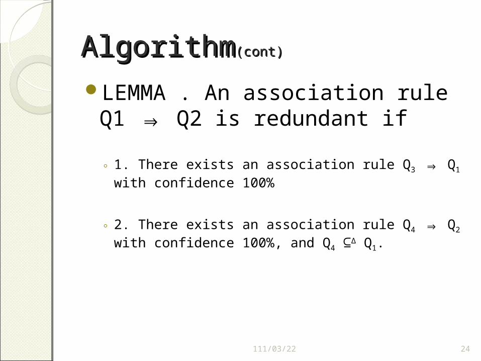
LEMMA . An association rule Q1 ⇒ Q2 is redundant if

◦ 1. There exists an association rule Q3 ⇒ Q1 with confidence 100%

◦ 2. There exists an association rule Q4 ⇒ Q2 with confidence 100%, and Q4 ⊆Δ Q1.

112/04/19 24

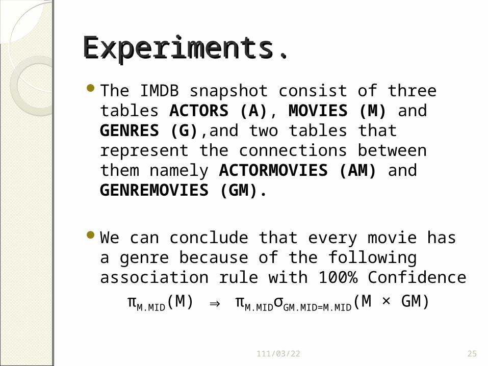
Experiments.Experiments.The IMDB snapshot consist of three

tables ACTORS (A), MOVIES (M) and GENRES (G),and two tables that represent the connections between them namely ACTORMOVIES (AM) and GENREMOVIES (GM).

We can conclude that every movie has a genre because of the following association rule with 100% Confidence

πM.MID(M) ⇒ πM.MIDσGM.MID=M.MID(M × GM)

112/04/19 25

ExperimentsExperiments(cont)(cont)

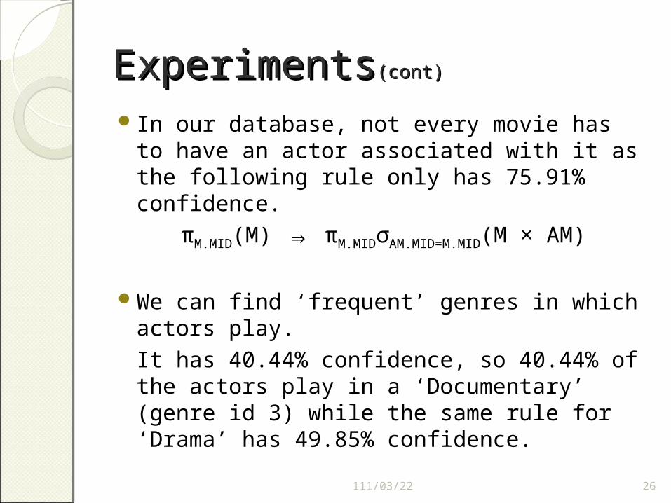
In our database, not every movie has to have an actor associated with it as the following rule only has 75.91% confidence.

πM.MID(M) ⇒ πM.MIDσAM.MID=M.MID(M × AM)

We can find ‘frequent’ genres in which actors play.It has 40.44% confidence, so 40.44% of the actors play in a ‘Documentary’ (genre id 3) while the same rule for ‘Drama’ has 49.85% confidence.

112/04/19 26

ExperimentsExperiments(cont)(cont)

81.60% of the actors in genre ‘Music’ (genre id 16) only play in one movie. But the same rule for genre ‘Crime’ has only49.87% confidence.

112/04/19 27

Conclusion.Conclusion.

112/04/19 28