Minimum Steiner Tree Construction∗

Gabriel Robins⋆ and Alexander Zelikovsky†

⋆Department of Computer Science, University of Virginia, Charlottesville, VA 22904robins@cs.virginia.edu, www.cs.virginia.edu/robins

†Department of Computer Science, Georgia State University, Atlanta, GA 30303alexz@cs.gsu.edu, www.cs.gsu.edu/~cscazz

1 Introduction

In optimizing the area of Very Large Scale Integrated (VLSI) layouts, circuit interconnections

should generally be realized with minimum total interconnect. This chapter addresses several

variations of the corresponding fundamental Steiner minimal tree (SMT) problem, where a given

set of pins is to be connected using minimum total wirelength. Steiner trees are important in

global routing and wirelength estimation [15], as well as in various non-VLSI applications such

as phylogenetic tree reconstruction in biology [48], network routing [61], and civil engineering,

among many other areas [21, 25, 26, 29, 51, 74].

In modern deep-submicron VLSI layout other criteria often dominate the routing objectives,

such as path lengths, skew, density, inductance, manufacturability, electromigration, reliability,

noise, power, non-Hanan topologies, signal integrity, three-dimensionality, alternate models, and

various combinations and tradeoffs of these [3, 5, 12, 27, 44, 45, 46, 50, 52, 57, 67, 70, 86].

However, large non-critical nets are still common in modern designs, and this chapter focuses

on the corresponding classical objective of wirelength/area minimization (which also minimizes

the total capacitance). This exposition is not an exhaustive survey on the Steiner problem,

about which hundreds of papers and several entire books were written [21, 25, 26, 29, 48, 51, 74].

Rather, it focuses on a few selected results and approaches to Steiner tree construction. A

∗This work was supported by a Packard Foundation Fellowship, by National Science Foundation Young Inves-tigator Award MIP-9457412, by a GSU Research Initiation Grant, by NSF grants CCR-9988331, CCF-0429737,CCF-0429735, and CNS-0716635, and by U.S. Civilian Research and Development Foundation grant MOM2-3049-CS-03.

broader overview of the field of computer-aided design of VLSI is given by several textbooks on

this subject [34, 71, 81, 84, 85].

Given a set P of n pins (i.e., terminals of a signal net), we seek to interconnect these points

using a minimual total amount of wire. This objective arises in VLSI minimum-area global rout-

ing, since VLSI minimum-spacing design rules induce an essentially linear relationship between

wirelength and wiring area. When all wires are “point-to-point”, with no intermediate junctions

other than points of P , the optimum solution is a minimum spanning tree (MST) over P , denoted

as MST (P ). However, we can usually introduce intermediate junctions, called Steiner points, in

connecting the points of P . The Steiner minimal tree problem can be formulated as follows.

The Steiner Minimal Tree (SMT) Problem: Given a set P of n points, determine a set S of

Steiner points such that the minimum spanning tree (MST) cost over P ∪ S is minimized.

An optimal solution to this problem is referred to as a Steiner minimal tree (or simply “Steiner

tree”) over P , denoted SMT (P ). An edge in a tree T has cost equal to the distance between

its endpoints, and the cost of T itself is the sum of its edge costs, denoted cost(T ). The wiring

cost between a pair of pins (x1, y1) and (x2, y2) in a VLSI layout is typically modeled by the

Manhattan, or rectilinear distance1:

dist((x1, y1), (x2, y2)) = (∆x) + (∆y) = |x1 − x2|+ |y1 − y2|

We will focus on the rectilinear Steiner minimal tree problem, where every edge is embedded

in the plane using a path of one or more alternating horizontal and vertical segments between its

endpoints. Figure 1 depicts an MST and an SMT for the same pointset in the Manhattan plane.

The bounding box of a pointset P denotes the smallest rectangle2 which contains all points of

P and whose sides are oriented parallel to the coordinate axes. If an edge between two points

is embedded with minimum possible wirelength, its routing segments will remain within the

bounding box induced by its endpoints.

1More recently, non-Manhattan interconnect architectures, such as “preferred direction” routing and λ-geometries, have been gaining popularity [19, 20, 21, 59, 64, 69, 83, 90, 94, 96]. However, most of the methodsdescribed in this chapter can be generalized to these other geometries and metrics, as well as to higher dimensions.

2Bounding “boxes” in non-Manhattan metrics/geometries have corresponding non-rectangular shapes, inducedby the underlying metric/geometry [21].

2

(a) (b)

Figure 1: (a) The minimum spanning tree (MST) and (b) the Steiner minimaltree (SMT) in the rectilinear plane. Hollow dots represent the original pointsetP , and solid dots represent Steiner points.

2 Historical Perspectives

The “Steiner problem” is named after the Swiss mathematician Jacob Steiner (1796-1863), who

solved and popularized the problem of joining three villages by a system of roads having minimum

total length [37] (he also addressed the general case of this problem, and made many fundamental

contributions to projective geometry). However, while Jacob Steiner’s work on this problem was

independent of its predecessors, about two centuries earlier Pierre de Fermat (1601-1665) proposed

this problem to Evangelista Torricelli (1608-1647), who solved it and passed it along to his student

Vincenzo Viviani (1622-1703), who in turn published his own solution as well as Torricelli’s in

1659 [91]. An even earlier (and presumably independent) published discussion of this problem,

is found in a 1647 book by the Italian mathematician Bonaventura Francesco Cavalieri (1598-

1647) [17]. Luckily, today we refer to this problem simply as the Steiner problem, instead of the

more accurate but considerably less wieldy title “the Fermat-Torricelli-Viviani-Cavalieri-Steiner

problem”.

More recent research progress on the Steiner minimal tree (SMT) problem has been historically

driven by several main results.

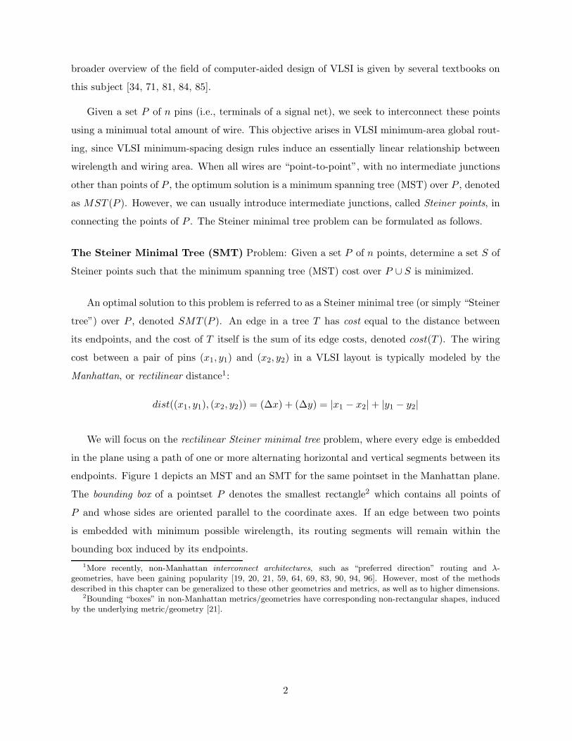
1. In 1966 Hanan [38] showed that for a pointset P there exists an SMT whose Steiner points S

are all chosen from the Hannan grid, namely the intersections of all the horizontal and ver-

tical lines passing through every point of P (see Figure 2). Snyder [88] generalized Hanan’s

theorem to all higher-dimensional Manhattan geometries; on the other hand, extensions of

Hanan’s theorem to λ-geometries are less straightforward [95].

3

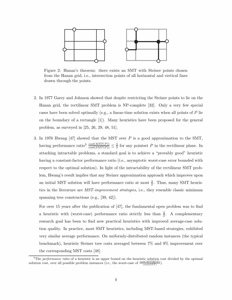
Figure 2: Hanan’s theorem: there exists an SMT with Steiner points chosenfrom the Hanan grid, i.e., intersection points of all horizontal and vertical linesdrawn through the points.

2. In 1977 Garey and Johnson showed that despite restricting the Steiner points to lie on the

Hanan grid, the rectilinear SMT problem is NP-complete [32]. Only a very few special

cases have been solved optimally (e.g., a linear-time solution exists when all points of P lie

on the boundary of a rectangle [1]). Many heuristics have been proposed for the general

problem, as surveyed in [25, 26, 29, 48, 51].

3. In 1976 Hwang [47] showed that the MST over P is a good approximation to the SMT,

having performance ratio3 cost(MST (P ))cost(SMT (P )) ≤ 3

2 for any pointset P in the rectilinear plane. In

attacking intractable problems, a standard goal is to achieve a “provably good” heuristic

having a constant-factor performance ratio (i.e., asymptotic worst-case error bounded with

respect to the optimal solution). In light of the intractability of the rectilinear SMT prob-

lem, Hwang’s result implies that any Steiner approximation approach which improves upon

an initial MST solution will have performance ratio at most 32 . Thus, many SMT heuris-

tics in the literature are MST-improvement strategies, i.e., they resemble classic minimum

spanning tree constructions (e.g., [39, 42]).

For over 15 years after the publication of [47], the fundamental open problem was to find

a heuristic with (worst-case) performance ratio strictly less than 32 . A complementary

research goal has been to find new practical heuristics with improved average-case solu-

tion quality. In practice, most SMT heuristics, including MST-based strategies, exhibited

very similar average performance. On uniformly-distributed random instances (the typical

benchmark), heuristic Steiner tree costs averaged between 7% and 9% improvement over

the corresponding MST costs [48].

3The performance ratio of a heuristic is an upper bound on the heuristic solution cost divided by the optimalsolution cost, over all possible problem instances (i.e., the worst-case of cost(APPROX)

cost(OPT )).

4

4. In 1990 Kahng and Robins have shown [54, 56, 57, 77] that any Steiner tree heuristic in

a general class of greedy MST-based methods has worst-case performance ratio arbitrarily

close to 32 , i.e., the MST for certain classes of pointsets is unimprovable. Thus, the 3

2 bound

is tight for a wide range of MST-based strategies in the rectilinear plane [56], which resolved

the performance ratios for a number of heuristics in the literature with previously unknown

worst-case behavior. Moreover, this established that in general, MST-based Steiner heuris-

tics (e.g., where MST edges are “flipped” within their bounding boxes) are unlikely to

achieve performance ratio better than 32 . Analogous constructions in higher d-dimensional

Manhattan geometry showed that all of these heuristics have performance ratio of at least

2d−1d

, which is bounded from above by 2 as the dimension grows [56, 57].

5. In 1992 Zelikovsky developed a rectilinear Steiner tree algorithm with a performance ratio

of 118 times optimal [97], the first heuristic provably better than the MST. His techniques

yield a general graph Steiner tree algorithm with a 116 performance ratio [98], the first

graph Steiner approximation proven to beat the MST-based graph Steiner heuristic of

Kou, Markowsky, and Berman [62]. This settled in the affirmative the longstanding open

question of whether there exists a polynomial-time rectilinear Steiner tree heuristic with

performance ratio < 32 , and whether there exists a polynomial-time graph Steiner tree

heuristic with performance ratio < 2.

In light of this sequence of developments, research on Steiner tree approximation has turned

away from MST-improvement heuristics. One of the earliest and most effective Steiner tree

approximation schemes to break away from the herd of MST-improvement shemes is the Iterated

1-Steiner (I1S) approach of Kahng and Robins [54, 55, 57, 77]. The I1S heuristic is simple, easy

to implement, generalizes naturally to any dimension and metric (including arbitrary weighted

graphs), and significantly outperforms previous approaches, as detailed below. The I1S algorithm

was subsequently proven to be the earliest published Steiner approximation method to have a

non-trivial performance ratio (of 1.5 times optimal) in quasi-bipartite graphs [79, 80].

3 The Iterated 1-Steiner (I1S) Approach

This section outlines the Iterated 1-Steiner heuristic [55, 57], which repeatedly finds optimum

single Steiner points for inclusion into the pointset. Given two pointsets A and B, we define the

MST savings of B with respect to A as:

5

∆MST (A,B) = cost(MST (A)) − cost(MST (A ∪B)).

Let H(P ) denote the Steiner candidate set, i.e., the intersection points of all horizontal and

vertical lines passing through points of P (as defined by Hanan’s theorem [38] - see Figure 2).

For any pointset P , a 1-Steiner point with respect to P is a point x ∈ H(P ) that maximizes

∆MST (P, {x}) > 0. Starting with a pointset P and a set S = ∅ of Steiner points, the Iterated

1-Steiner (I1S) method repeatedly finds a 1-Steiner point x for P ∪S and sets S ← S ∪{x}. The

cost of MST (P ∪ S) will decrease with each added point, and the construction terminates when

there no longer exists any point x with ∆MST (P ∪ S, {x}) > 0.

An optimal Steiner tree over n points has at most n−2 Steiner points of degree at least 3 (this

follows from simple degree arguments [35]). However, the I1S method can (or rare occasions) add

more than n− 2 Steiner points. Therefore, at each iteration we eliminate any extraneous Steiner

points which have degree ≤ 2 in the MST over P ∪S (since such points can not contribute to the

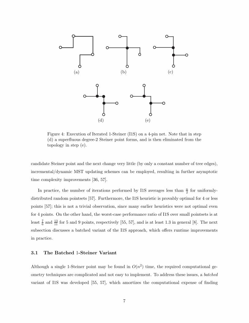
tree cost savings). Figure 3 formally describes the algorithm, and Figure 4 illustrates a sample

execution.

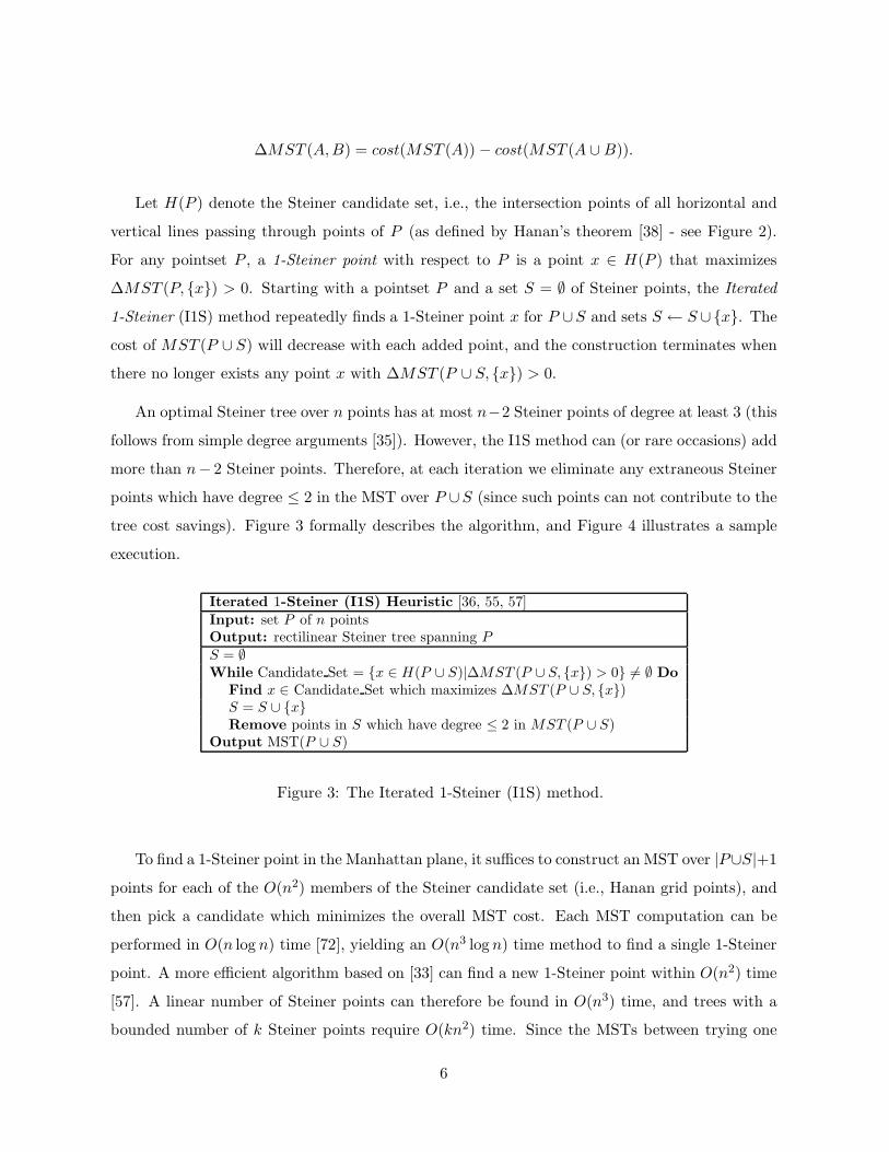
Iterated 1-Steiner (I1S) Heuristic [36, 55, 57]Input: set P of n pointsOutput: rectilinear Steiner tree spanning P

S = ∅While Candidate Set = {x ∈ H(P ∪ S)|∆MST (P ∪ S, {x}) > 0} 6= ∅ Do

Find x ∈ Candidate Set which maximizes ∆MST (P ∪ S, {x})S = S ∪ {x}Remove points in S which have degree ≤ 2 in MST (P ∪ S)

Output MST(P ∪ S)

Figure 3: The Iterated 1-Steiner (I1S) method.

To find a 1-Steiner point in the Manhattan plane, it suffices to construct an MST over |P∪S|+1

points for each of the O(n2) members of the Steiner candidate set (i.e., Hanan grid points), and

then pick a candidate which minimizes the overall MST cost. Each MST computation can be

performed in O(n log n) time [72], yielding an O(n3 log n) time method to find a single 1-Steiner

point. A more efficient algorithm based on [33] can find a new 1-Steiner point within O(n2) time

[57]. A linear number of Steiner points can therefore be found in O(n3) time, and trees with a

bounded number of k Steiner points require O(kn2) time. Since the MSTs between trying one

6

(a) (b) (c)

(d) (e)

Figure 4: Execution of Iterated 1-Steiner (I1S) on a 4-pin net. Note that in step(d) a superfluous degree-2 Steiner point forms, and is then eliminated from thetopology in step (e).

candidate Steiner point and the next change very little (by only a constant number of tree edges),

incremental/dynamic MST updating schemes can be employed, resulting in further asymptotic

time complexity improvements [36, 57].

In practice, the number of iterations performed by I1S averages less than n2 for uniformly-

distributed random pointsets [57]. Furthermore, the I1S heuristic is provably optimal for 4 or less

points [57]; this is not a trivial observation, since many earlier heuristics were not optimal even

for 4 points. On the other hand, the worst-case performance ratio of I1S over small pointsets is at

least 76 and 13

11 for 5 and 9 points, respectively [55, 57], and is at least 1.3 in general [8]. The next

subsection discusses a batched variant of the I1S approach, which offers runtime improvements

in practice.

3.1 The Batched 1-Steiner Variant

Although a single 1-Steiner point may be found in O(n2) time, the required computational ge-

ometry techniques are complicated and not easy to implement. To address these issues, a batched

variant of I1S was developed [55, 57], which amortizes the computational expense of finding

7

1-Steiner points by adding as many “independent” 1-Steiner points as possible in every round.

The Batched 1-Steiner (B1S) variant computes ∆MST (P, {x}) for each candidate Steiner

point x ∈ H(P ) (i.e., the Hanan grid candidate points). Two candidate Steiner points x and y

are independent if:

∆MST (P, {x}) + ∆MST (P, {y}) ≤ ∆MST (P, {x, y}),

introducing each of the two 1-Steiner points does not reduce the potential gain in MST cost

relative of the other 1-Steiner point. Given pointset P and a set of Steiner points S, each round

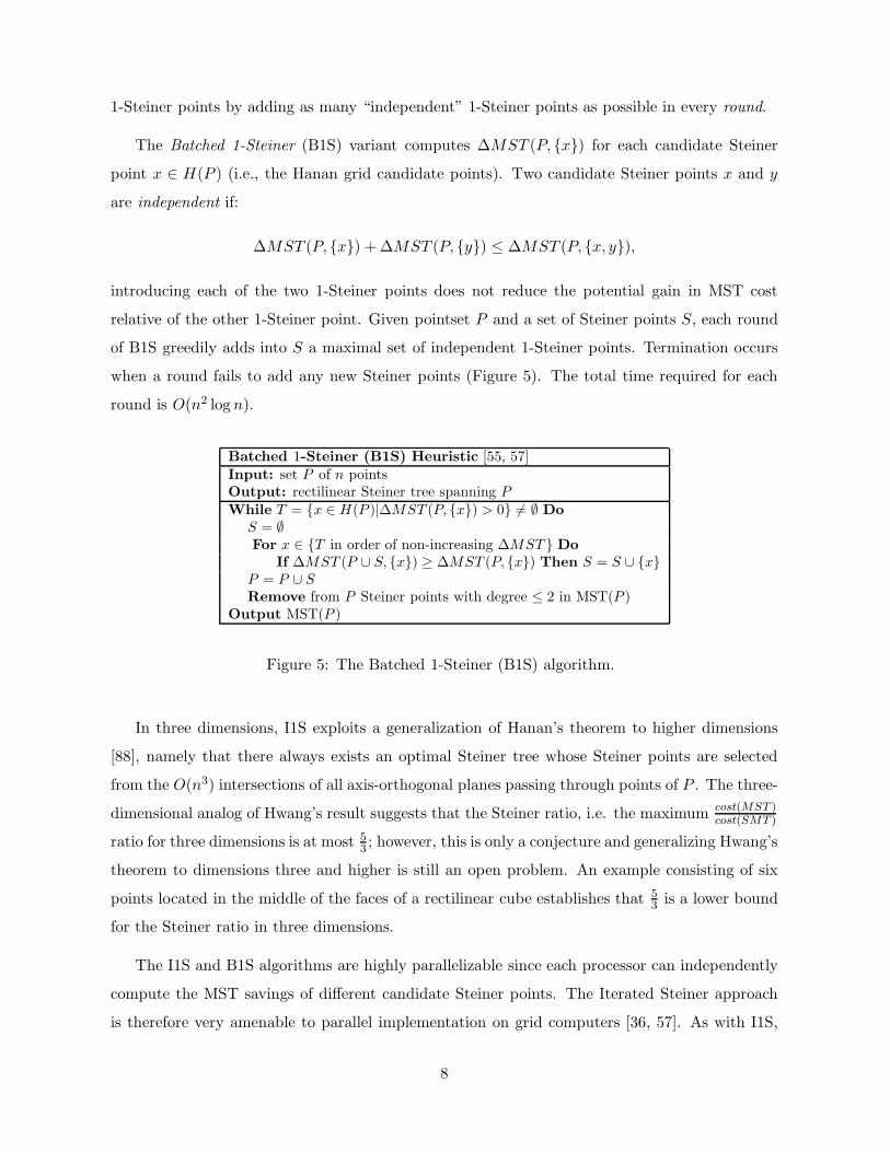
of B1S greedily adds into S a maximal set of independent 1-Steiner points. Termination occurs

when a round fails to add any new Steiner points (Figure 5). The total time required for each

round is O(n2 log n).

Batched 1-Steiner (B1S) Heuristic [55, 57]Input: set P of n pointsOutput: rectilinear Steiner tree spanning P

While T = {x ∈ H(P )|∆MST (P, {x}) > 0} 6= ∅ DoS = ∅For x ∈ {T in order of non-increasing ∆MST } Do

If ∆MST (P ∪ S, {x}) ≥ ∆MST (P, {x}) Then S = S ∪ {x}P = P ∪ S

Remove from P Steiner points with degree ≤ 2 in MST(P )Output MST(P )

Figure 5: The Batched 1-Steiner (B1S) algorithm.

In three dimensions, I1S exploits a generalization of Hanan’s theorem to higher dimensions

[88], namely that there always exists an optimal Steiner tree whose Steiner points are selected

from the O(n3) intersections of all axis-orthogonal planes passing through points of P . The three-

dimensional analog of Hwang’s result suggests that the Steiner ratio, i.e. the maximum cost(MST )cost(SMT )

ratio for three dimensions is at most 53 ; however, this is only a conjecture and generalizing Hwang’s

theorem to dimensions three and higher is still an open problem. An example consisting of six

points located in the middle of the faces of a rectilinear cube establishes that 53 is a lower bound

for the Steiner ratio in three dimensions.

The I1S and B1S algorithms are highly parallelizable since each processor can independently

compute the MST savings of different candidate Steiner points. The Iterated Steiner approach

is therefore very amenable to parallel implementation on grid computers [36, 57]. As with I1S,

8

the time complexity and practical runtime of B1S can be further improved using incremental /

dynamic MST update techniques [16]. Moreover, by exploiting tighter bounds on the maximum

MST degree in the rectilinear metric4, further runtime improvements can be obtained [36, 57, 78].

3.2 Empirical Performance of Iterated 1-Steiner

In benchmark tests, I1S and B1S compare very favorably with optimal Steiner tree algorithms,

such as those of Salowe and Warme [82, 92] on random uniformly distributed pointsets (i.e., the

standard testbed for Steiner tree heuristics [48]). Both I1S and B1S exhibit very similar average

performance in terms of solution quality, approaching 11% average improvement over MST cost,

which is on average less than half a percent from optimal. Moreover, I1S and B1S produce

optimal solutions on 90% of all random 8-point instances (and on more than half of all random

15-point instances). For n = 30 points, I1S and B1S are on average only about 0.3% away from

optimal, and yield optimal solutions in about one quarter of the cases [36, 57]. I1S and B1S also

perform similarly well in three dimensions and in other Lk norms [36, 57].

Empirical experiments also indicate that the number of rounds required by B1S grows very

slowly (i.e., apparently logarithmically) with the number of points [36, 57]. For example, on sets

of 300 points the average number of B1S rounds is only 2.5, and was never observed to be more

than 5 on any instance. As expected, over 95% of the total tree cost improvement occurs in the

first B1S round, and over 99% of the total improvement occurs in the first two rounds [36, 57].

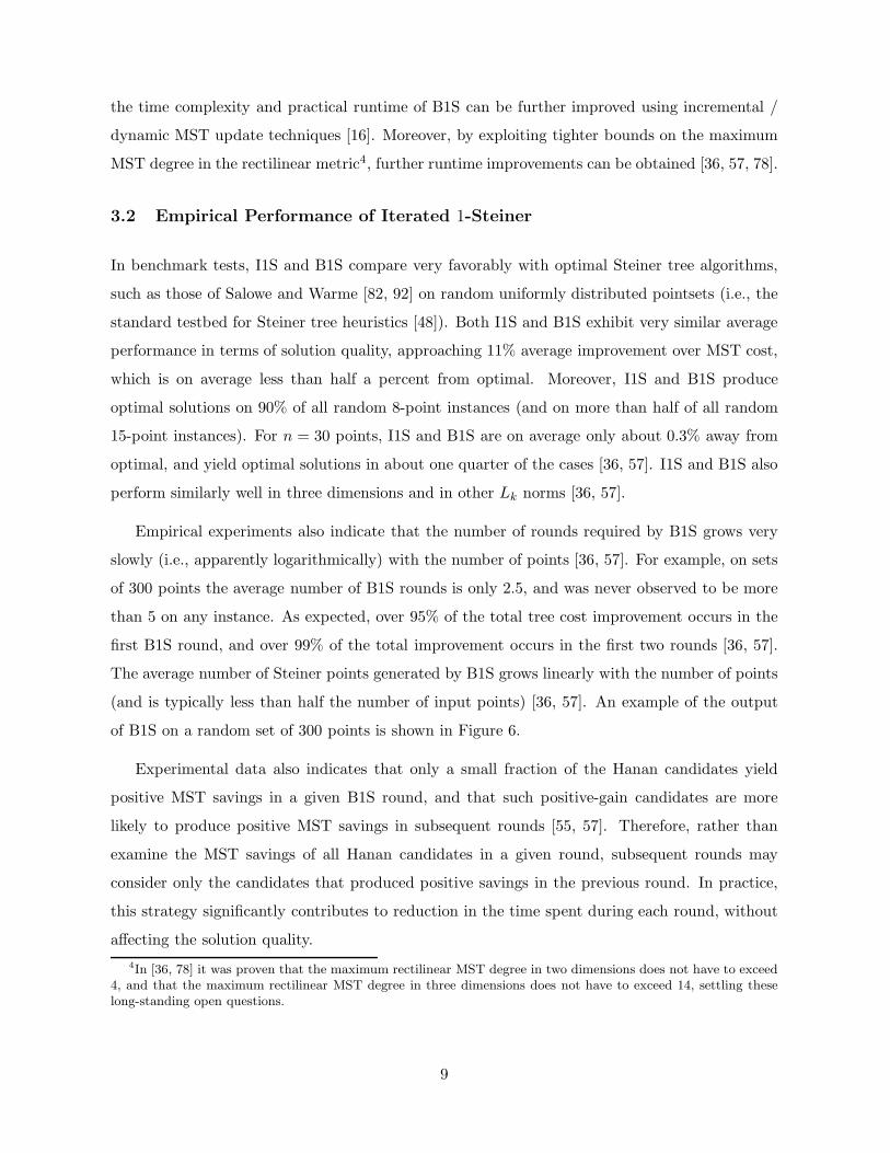
The average number of Steiner points generated by B1S grows linearly with the number of points

(and is typically less than half the number of input points) [36, 57]. An example of the output

of B1S on a random set of 300 points is shown in Figure 6.

Experimental data also indicates that only a small fraction of the Hanan candidates yield

positive MST savings in a given B1S round, and that such positive-gain candidates are more

likely to produce positive MST savings in subsequent rounds [55, 57]. Therefore, rather than

examine the MST savings of all Hanan candidates in a given round, subsequent rounds may

consider only the candidates that produced positive savings in the previous round. In practice,

this strategy significantly contributes to reduction in the time spent during each round, without

affecting the solution quality.

4In [36, 78] it was proven that the maximum rectilinear MST degree in two dimensions does not have to exceed4, and that the maximum rectilinear MST degree in three dimensions does not have to exceed 14, settling theselong-standing open questions.

9

Figure 6: An example of the output of B1S on a random set of 300 points (hollowdots). The Steiner points produced by B1S are denoted by solid dots.

3.3 Generalization of I1S to Steiner Arborescences

The Iterated 1-Steiner algorithmic template also generalizes to produce Steiner arborescences,

i.e., shortest-paths trees with minimum wirelength, which are known to yield high-performance

critical net routings [45]. The Iterated Dominance (IDOM) graph arborescence heuristic of [2]

recapitulates the Iterated 1-Steiner strategy, by greedily iterating over a given spanning arbores-

cence construction. To construct a Steiner arborescence, the IDOM heuristic repeatedly finds

10

Steiner candidates that reduce the overall spanning arborescence cost by the greatest amount,

and includes them into the growing set of Steiner nodes. The reason that a spanning arbores-

cence criterion is used to drive the Steiner arborescence construction, is that the former is easy

to compute [2], while the latter is NP-complete [87]. Arborescence constructions are described in

greater detail in another chapter.

4 Steiner Trees in Graphs

A more general version of the Steiner problem arises when interpoint distances can be arbitrary,

rather than induced by an underlying metric or a particular geometry. This topological, or graph-

based version of the Steiner problem occurs in practice when we wish to route a signal net in the

presence of obstacles, congestion, or variable-cost routing resources, such as in field-programmable

gate arrays [2]. More formally, given an arbitrary weighted graph with a distinguished vertex

subset, the Graph Steiner Tree Problem seeks a minimum-cost subtree spanning the distinguished

vertices.

The Graph Steiner Minimal Tree (GSMT) problem: Given a weighted graph G = (V,E),

and a distinguished set of nodes N ⊆ V , find a minimum-cost spanning tree T = (V ′, E′) with

N ⊆ V ′ ⊆ V and E′ ⊆ E.

In particular, any node in V − N can serve as a potential Steiner point. As usual, each

graph edge eij ∈ E has a real-valued weight wij , and the cost of a tree (or any subgraph) is the

sum of the weights of its edges. The GSMT problem is NP-complete, even in the Euclidean or

rectilinear metrics [32], since the geometric SMT problems are special cases of the general graph

SMT problem. The method of Kou, Markowsky and Berman (KMB) [62] was the first provably-

good heuristic to solve the GSMT problem in polynomial time with approximation ratio of twice

the optimal.

4.1 Graph Generalization of Iterated 1-Steiner

The Iterated 1-Steiner approach generalizes to solve the Steiner problem in arbitrary weighted

graphs, by combining the geometric I1S heuristic with the KMB [62] graph Steiner algorithm

[2, 57]. The resulting hybrid method inherits the good average-case performance of the Iterated

1-Steiner method, while also enjoying the error-bounded performance of the KMB algorithm. We

refer to this hybrid method as the Graph Iterated 1-Steiner (GI1S) algorithm. The GI1S method

11

is essentially an adaptation of I1S to graphs, where the “MST” in the inner loop is replaced with

the KMB construction. That is, instead of using an “MST” subroutine to determine the “savings”

of a candidate Steiner point/node, we use the KMB (or any other) approximation algorithm for

this purpose. Thus, given a graph G = (V,E), a set N ⊆ V , and a set S of potential Steiner

points, we define the following:

∆KMB(N,S) = cost(KMB(N))− cost(KMB(N ∪ S))

Thus, the GI1S template (Figure 7) repeatedly finds Steiner node candidates that reduce the

overall KMB cost and includes them into the growing set of Steiner nodes S. The cost of the

KMB tree over N∪S will decrease with each added Steiner node, and the construction terminates

when there is no x ∈ V with ∆KMB(N ∪ S, {x}) > 0.

Graph Iterated 1-Steiner (GI1S) Heuristic [2, 57]Input: weighted graph G = (V, E) and a set N ⊆ V

Output: low-cost tree T ′ = (V ′, E′) spanning N (i.e. N ⊆ V ′ ⊆ V and E′ ⊆ E)S = ∅While T = {x ∈ V −N | ∆KMB(N ∪ S, {x}) > 0} 6= ∅ Do

Find x ∈ T with maximum ∆KMB(N ∪ S, {x})S = S ∪ {x}

Return KMB(N ∪ S)

Figure 7: The Graph Iterated 1-Steiner algorithm (GI1S).

The approximation ratio for GI1S is 2 · (1− 1L) ≤ 2 times optimal, where L is the number of

leaves in the resulting tree. This follows from the KMB bound and from the fact that the cost

of the GI1S construction cannot exceed that of the KMB construction [2, 57]. If |N | ≤ 3 (e.g., a

VLSI signal net with three or fewer terminals - a very common occurrence in VLSI layouts), GI1S

is guaranteed to find an optimal solution. Although the worst-case performance ratio of GI1S is

the same as that of KMB, in practice GI1S significantly outperforms KMB in terms of solution

quality [2]. Given a faster implementation of the KMB method [93], the GI1S algorithm can be

implemented within time O(|N | · |G| + |N |4 log |N |), where |N | ≤ |V | is the number of nodes

to be spanned and |G| = |V | + |E| is the size of the graph. Moreover, like with I1S, the GI1S

approach can be “batched”, and incremental/dynamic MST computations [16] can be exploited,

resulting in further runtime improvements.

Note that the GI1S template above can be viewed as an Iterated KMB (IKMB) construction,

12

and that KMB inside the inner loop may be replaced with any other graph Steiner approxi-

mation heuristic, such as that of Zelikovsky (ZEL) [98], yielding an Iterated Zelikovsky (IZEL)

heuristic. IZEL has the same theoretical performance bound as ZEL, namely 116 , but provides

imroved solutions in practice. Experiments have shown that these heuristics in order of increas-

ing average solution quality are KMB < ZEL < IKMB < IZEL [2]. In general, iterating a given

Steiner approximation heuristic greedily is an effective general mechanism to improve empirical

performance without sacrificing the theoretical performance bounds.

4.2 The Loss-Contracting Approach

For arbitrary weighted graphs, the best Steiner approximation ratio achievable within polynomial

time was steadily improved from 2 down to 1.5493 in a series of papers [89, 62, 98, 10, 73, 58, 43,

79]. On the negative side, it is known that unless P = NP , the Steiner Tree Problem in general

graphs cannot be approximated within a factor of 1 + ǫ for sufficiently small ǫ > 0 [11]. More

recently, an improved non-approximability lower bound of 9695 for the graph Steiner problem was

proved in [22].

The graph Steiner tree heuristic with the best-known performance ratio, approaching 1+ ln 32 ≈

1.5493, was given by Robins and Zelikovsky [79, 80]. This approach, called the Loss-Contracting

Algorithm (LCA), proceeds by adding full components to a growing solution, based on their

relative cost savings. A full component is a Steiner tree over a terminal subset in which all of the

terminals are leaves (see Figure 8(a)). Any Steiner tree can be decomposed into full components

by splitting all the non-leaf terminals (we assume that any full component has its own copy of

each Steiner point, so that full components chosen by the algorithm do not share Steiner points).

A Steiner tree which does not contain any Steiner points (i.e., where each full component consists

of a single edge), is called a terminal-spanning tree. The LCA algorithm computes relative cost

savings with respect to a “shrinking” terminal-spanning tree.

All previous graph Steiner heuristics (except [10]) with provably good approximation ratios

repeatedly choose appropriate full components and then contract them in order to form the

overall solution. However, this strategy does not allow the discarding of an already-accepted full

component, even if it turns out later that a better full component conflicts with a previously

accepted component (two components conflict if they share at least two terminals).

The intuition behind the Loss-Contracting Algorithm is to contract as little as possible so that

13

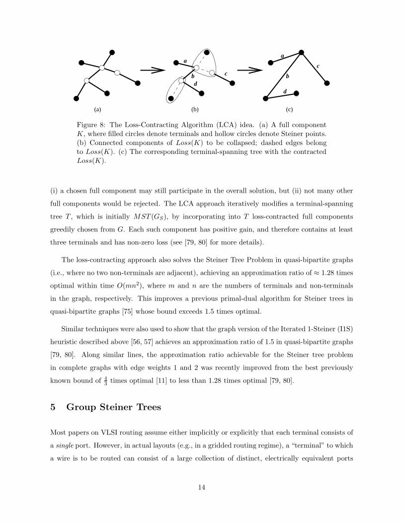
a

d

bd

b c

a

(c)(b)(a)

c

Figure 8: The Loss-Contracting Algorithm (LCA) idea. (a) A full componentK, where filled circles denote terminals and hollow circles denote Steiner points.(b) Connected components of Loss(K) to be collapsed; dashed edges belongto Loss(K). (c) The corresponding terminal-spanning tree with the contractedLoss(K).

(i) a chosen full component may still participate in the overall solution, but (ii) not many other

full components would be rejected. The LCA approach iteratively modifies a terminal-spanning

tree T , which is initially MST (GS), by incorporating into T loss-contracted full components

greedily chosen from G. Each such component has positive gain, and therefore contains at least

three terminals and has non-zero loss (see [79, 80] for more details).

The loss-contracting approach also solves the Steiner Tree Problem in quasi-bipartite graphs

(i.e., where no two non-terminals are adjacent), achieving an approximation ratio of ≈ 1.28 times

optimal within time O(mn2), where m and n are the numbers of terminals and non-terminals

in the graph, respectively. This improves a previous primal-dual algorithm for Steiner trees in

quasi-bipartite graphs [75] whose bound exceeds 1.5 times optimal.

Similar techniques were also used to show that the graph version of the Iterated 1-Steiner (I1S)

heuristic described above [56, 57] achieves an approximation ratio of 1.5 in quasi-bipartite graphs

[79, 80]. Along similar lines, the approximation ratio achievable for the Steiner tree problem

in complete graphs with edge weights 1 and 2 was recently improved from the best previously

known bound of 43 times optimal [11] to less than 1.28 times optimal [79, 80].

5 Group Steiner Trees

Most papers on VLSI routing assume either implicitly or explicitly that each terminal consists of

a single port. However, in actual layouts (e.g., in a gridded routing regime), a “terminal” to which

a wire is to be routed can consist of a large collection of distinct, electrically equivalent ports

14

[7, 41, 40]. Even though a wire may connect to any one of these ports, this degree of freedom is

often not fully exploited in routing or in wiring estimation. This section addresses the general

problem of minimum-cost Steiner tree construction in the presence of multi-port terminals, where

rather than spanning a set of nodes, the objective is to connect groups of nodes. This is also

known as the Group Steiner Problem (Figure 9), formulated as follows:

The Group Steiner Problem [48, 76]: given a weighted graph G = (V,E) and a family

N = {N1, ..., Nk} of k disjoint groups of nodes Ni ⊆ V , find a minimum-cost spanning tree in G

containing at least one node from each group Ni.

As in the classical Steiner problem, we are allowed to include optional Steiner nodes in order

to reduce the cost of the tree interconnecting the groups of N . The problem of interconnecting a

net with multi-port terminals is a direct generalization of the NP-complete Steiner problem (i.e.,

in the classical Steiner problem each terminal contains exactly one port), and is therefore itself

NP-complete.

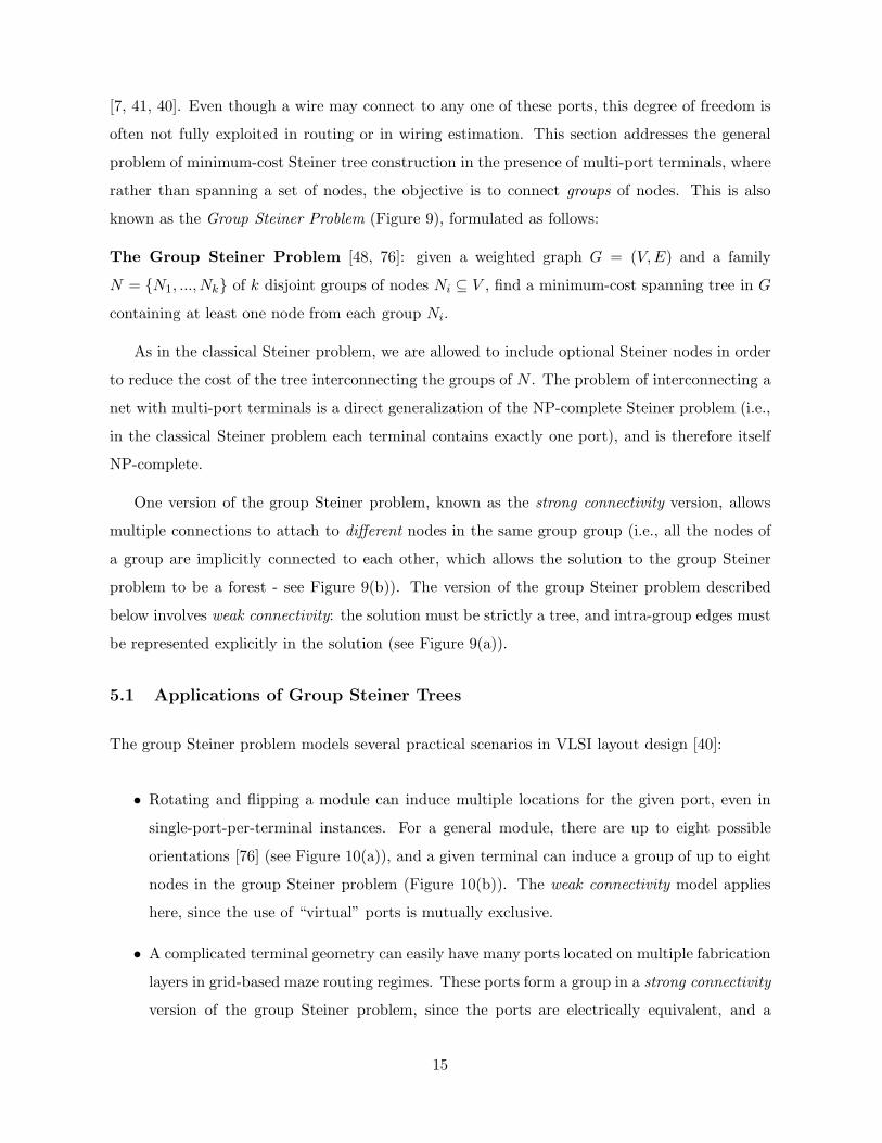
One version of the group Steiner problem, known as the strong connectivity version, allows

multiple connections to attach to different nodes in the same group group (i.e., all the nodes of

a group are implicitly connected to each other, which allows the solution to the group Steiner

problem to be a forest - see Figure 9(b)). The version of the group Steiner problem described

below involves weak connectivity: the solution must be strictly a tree, and intra-group edges must

be represented explicitly in the solution (see Figure 9(a)).

5.1 Applications of Group Steiner Trees

The group Steiner problem models several practical scenarios in VLSI layout design [40]:

• Rotating and flipping a module can induce multiple locations for the given port, even in

single-port-per-terminal instances. For a general module, there are up to eight possible

orientations [76] (see Figure 10(a)), and a given terminal can induce a group of up to eight

nodes in the group Steiner problem (Figure 10(b)). The weak connectivity model applies

here, since the use of “virtual” ports is mutually exclusive.

• A complicated terminal geometry can easily have many ports located on multiple fabrication

layers in grid-based maze routing regimes. These ports form a group in a strong connectivity

version of the group Steiner problem, since the ports are electrically equivalent, and a

15

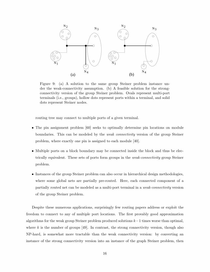
(b)(a)

N1

N4

3N2N3N2N

1N

4N

Figure 9: (a) A solution to the same group Steiner problem instance un-der the weak-connectivity assumption. (b) A feasible solution for the strong-connectivity version of the group Steiner problem. Ovals represent multi-portterminals (i.e., groups), hollow dots represent ports within a terminal, and soliddots represent Steiner nodes.

routing tree may connect to multiple ports of a given terminal.

• The pin assignment problem [60] seeks to optimally determine pin locations on module

boundaries. This can be modeled by the weak connectivity version of the group Steiner

problem, where exactly one pin is assigned to each module [40].

• Multiple ports on a block boundary may be connected inside the block and thus be elec-

trically equivalent. These sets of ports form groups in the weak-connectivity group Steiner

problem.

• Instances of the group Steiner problem can also occur in hierarchical design methodologies,

where some global nets are partially pre-routed. Here, each connected component of a

partially routed net can be modeled as a multi-port terminal in a weak-connectivity version

of the group Steiner problem.

Despite these numerous applications, surprisingly few routing papers address or exploit the

freedom to connect to any of multiple port locations. The first provably good approximation

algorithms for the weak group Steiner problem produced solutions k−1 times worse than optimal,

where k is the number of groups [49]. In contrast, the strong connectivity version, though also

NP-hard, is somewhat more tractable than the weak connectivity version: by converting an

instance of the strong connectivity version into an instance of the graph Steiner problem, then

16

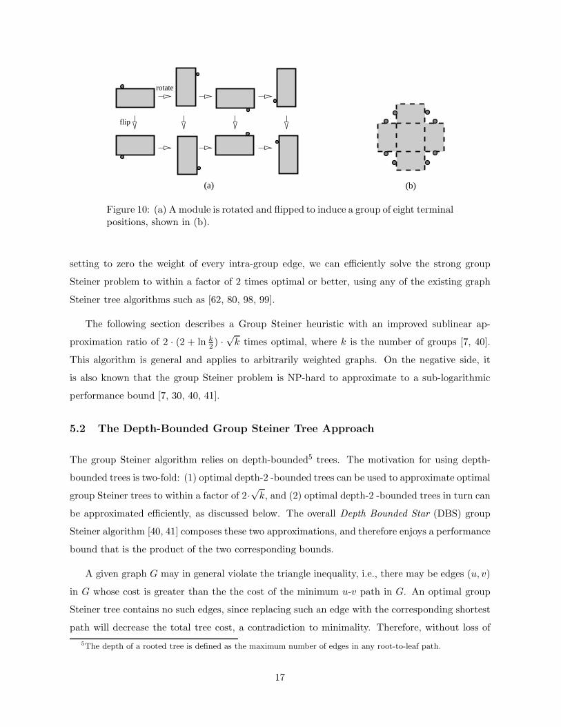
(b)

rotate

flip

(a)

Figure 10: (a) A module is rotated and flipped to induce a group of eight terminalpositions, shown in (b).

setting to zero the weight of every intra-group edge, we can efficiently solve the strong group

Steiner problem to within a factor of 2 times optimal or better, using any of the existing graph

Steiner tree algorithms such as [62, 80, 98, 99].

The following section describes a Group Steiner heuristic with an improved sublinear ap-

proximation ratio of 2 · (2 + ln k2 ) ·√

k times optimal, where k is the number of groups [7, 40].

This algorithm is general and applies to arbitrarily weighted graphs. On the negative side, it

is also known that the group Steiner problem is NP-hard to approximate to a sub-logarithmic

performance bound [7, 30, 40, 41].

5.2 The Depth-Bounded Group Steiner Tree Approach

The group Steiner algorithm relies on depth-bounded5 trees. The motivation for using depth-

bounded trees is two-fold: (1) optimal depth-2 -bounded trees can be used to approximate optimal

group Steiner trees to within a factor of 2·√

k, and (2) optimal depth-2 -bounded trees in turn can

be approximated efficiently, as discussed below. The overall Depth Bounded Star (DBS) group

Steiner algorithm [40, 41] composes these two approximations, and therefore enjoys a performance

bound that is the product of the two corresponding bounds.

A given graph G may in general violate the triangle inequality, i.e., there may be edges (u, v)

in G whose cost is greater than the the cost of the minimum u-v path in G. An optimal group

Steiner tree contains no such edges, since replacing such an edge with the corresponding shortest

path will decrease the total tree cost, a contradiction to minimality. Therefore, without loss of

5The depth of a rooted tree is defined as the maximum number of edges in any root-to-leaf path.

17

generality, we replace G by its metric closure, defined as a complete graph where the cost of each

edge (u, v) is equal to the cost of the minimum u-v path in G.

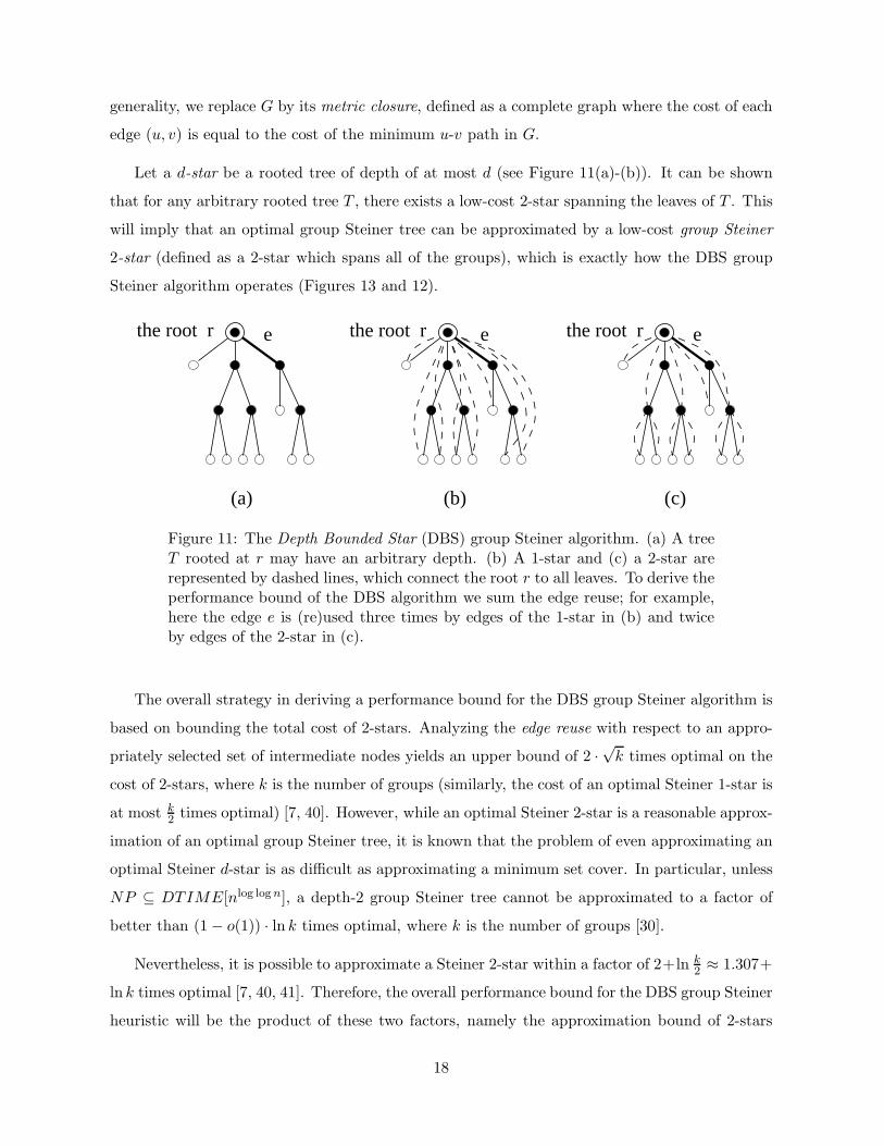
Let a d-star be a rooted tree of depth of at most d (see Figure 11(a)-(b)). It can be shown

that for any arbitrary rooted tree T , there exists a low-cost 2-star spanning the leaves of T . This

will imply that an optimal group Steiner tree can be approximated by a low-cost group Steiner

2-star (defined as a 2-star which spans all of the groups), which is exactly how the DBS group

Steiner algorithm operates (Figures 13 and 12).

e

(a) (b)

the root r the root r the root r

(c)

ee

Figure 11: The Depth Bounded Star (DBS) group Steiner algorithm. (a) A treeT rooted at r may have an arbitrary depth. (b) A 1-star and (c) a 2-star arerepresented by dashed lines, which connect the root r to all leaves. To derive theperformance bound of the DBS algorithm we sum the edge reuse; for example,here the edge e is (re)used three times by edges of the 1-star in (b) and twiceby edges of the 2-star in (c).

The overall strategy in deriving a performance bound for the DBS group Steiner algorithm is

based on bounding the total cost of 2-stars. Analyzing the edge reuse with respect to an appro-

priately selected set of intermediate nodes yields an upper bound of 2 ·√

k times optimal on the

cost of 2-stars, where k is the number of groups (similarly, the cost of an optimal Steiner 1-star is

at most k2 times optimal) [7, 40]. However, while an optimal Steiner 2-star is a reasonable approx-

imation of an optimal group Steiner tree, it is known that the problem of even approximating an

optimal Steiner d-star is as difficult as approximating a minimum set cover. In particular, unless

NP ⊆ DTIME[nlog log n], a depth-2 group Steiner tree cannot be approximated to a factor of

better than (1− o(1)) · ln k times optimal, where k is the number of groups [30].

Nevertheless, it is possible to approximate a Steiner 2-star within a factor of 2+ln k2 ≈ 1.307+

ln k times optimal [7, 40, 41]. Therefore, the overall performance bound for the DBS group Steiner

heuristic will be the product of these two factors, namely the approximation bound of 2-stars

18

with respect to optimal, times the bound with which 2-stars can themselves be approximated.

The DBS group Steiner heuristic (Figures 12 and 13) therefore solves the group Steiner minimal

tree problem with performance ratio 2 · (2 + ln k2 ) ·√

k, where k is the number of groups.

Depth-Bounded Star (DBS) Group Steiner Algorithm [7, 40, 41]Input: Weighted graph G = (V, E), a family N

of k disjoint groups N1, . . . , Nk ⊆ V

Output: A low-cost tree Approx spanningat least one vertex from each group Ni

For each node r ∈ V doFind a low-cost 2-star Approx2(r) rooted at r

intersecting each group Ni, i = 1, ..., k

Output the least-cost 2-star Approx,i.e. cost(Approx) = minr∈V cost(Approx2(r))

Figure 12: The Depth-Bounded Star (DBS) approximation algorithm for thegroup Steiner problem on arbitrary weighted graphs produces a low-cost Steiner2-star.

5.3 Time Complexity of the DBS Group Steiner Algorithm

The time complexity of computing minimum-norm partial stars (a subroutine in the DBS algo-

rithm) is O(|V | ·k · log k), where k is the number of groups. Approximating rooted 2-stars requires

O(|V | ·k2 · log k) time. The total runtime of the overall Depth-Bounded Star (DBS) group Steiner

heuristic (Figures 12 and 13) is therefore O(τ + |V |2 ·k2 · log k), where k is the number of groups,

and τ is the time complexity of computing all-pairs graph shortest paths.

A practical enhancement to the runtime of the DBS algorithm entails computing a group

minimum spanning tree instead of a group Steiner minimal tree (that is, computing a minimum

spanning tree for a set of nodes containing exactly one port from each group). It can be shown

that the optimal group minimum spanning tree is at most twice as long as the optimal group

Steiner minimal tree. Thus, in approximating the group Steiner minimal tree by a group minimum

spanning tree, only a factor of 2 is lost, which does not asymptotically increase the overall solution

quality bound of 2 · (2 + ln k2 ) ·√

k times optimal, yet yields substantial savings in runtime.

5.4 Degenerate Group Steiner Instances

While solving the group Steiner problem, optimizing degenerate groups (i.e. groups of size 1) as

a special case can yield substantial improvements in solution quality as well as in runtime. The

19

(c)

(b)

(a)

(e)

(f)

(d)

r

r

r

r

r

r

Figure 13: Given an instance of the group Steiner problem, for each possibleroot r, the Depth-Bounded Star (DBS) heuristic: (a) finds the optimal 1-star,(b) finds the minimum-norm partial star (shaded region), (c) stores this starin the solution and removes its groups from future consideration, (d) finds thenext minimum-norm partial star (shaded region), (e) repeats step (c) for thenew partial star, and finally (f) finds the last minimum-norm partial star andoutputs the union of all stored partial stars.

degenerate groups by themselves induce an instance of the classic Steiner problem, and such an

instance can be approximated efficiently with a constant performance ratio. Thus, to solve the

20

SMT problem for degenerate groups, we may choose a provably-good heuristic from among the

numerous existing ones [9, 36, 55, 57, 62, 79, 80, 98]. For example, in time O(|V |3) we may find

a Steiner tree which is at most 116 times optimal [99]. All that remains now is connecting the

Steiner minimal tree over the degenerate groups with a tree spanning the other, non-degenerate

groups, without degrading the overall performance ratio.

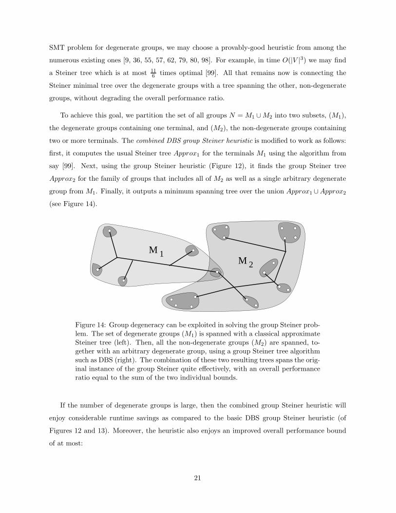
To achieve this goal, we partition the set of all groups N = M1 ∪M2 into two subsets, (M1),

the degenerate groups containing one terminal, and (M2), the non-degenerate groups containing

two or more terminals. The combined DBS group Steiner heuristic is modified to work as follows:

first, it computes the usual Steiner tree Approx1 for the terminals M1 using the algorithm from

say [99]. Next, using the group Steiner heuristic (Figure 12), it finds the group Steiner tree

Approx2 for the family of groups that includes all of M2 as well as a single arbitrary degenerate

group from M1. Finally, it outputs a minimum spanning tree over the union Approx1 ∪Approx2

(see Figure 14).

MM 2

1

Figure 14: Group degeneracy can be exploited in solving the group Steiner prob-lem. The set of degenerate groups (M1) is spanned with a classical approximateSteiner tree (left). Then, all the non-degenerate groups (M2) are spanned, to-gether with an arbitrary degenerate group, using a group Steiner tree algorithmsuch as DBS (right). The combination of these two resulting trees spans the orig-inal instance of the group Steiner quite effectively, with an overall performanceratio equal to the sum of the two individual bounds.

If the number of degenerate groups is large, then the combined group Steiner heuristic will

enjoy considerable runtime savings as compared to the basic DBS group Steiner heuristic (of

Figures 12 and 13). Moreover, the heuristic also enjoys an improved overall performance bound

of at most:

21

11

6+ 2 · (2 + ln

|M2|+ 1

2) ·

√

|M2|+ 1

where M2 is the set of degenerate groups of size 2 or more. In particular, if the number of

non-degenerate groups is bounded by a constant independently of the total number of nodes in

the graph (i.e., |M2| = O(1)), then the above hybrid DBS algorithm will solve such instances of

the group Steiner problem within a constant factor of optimal.

5.5 Bounded-Radius Group Steiner Trees

The objective of delay-minimization can induce wiring geometries that are substantially different

from those dictated by an optimal-area objective, particularly in deep submicron regimes. This

has motivated a number of bounded-radius6 routing constructions [4, 28, 57]. The basic group

Steiner tree approach can be easily extended to a bounded-radius construction, thereby yielding

routing trees with source-to-sink pathlengths bounded by a user-specified parameter.

For example, the tree produced by the DBS group Steiner algorithm above (Figures 12 and

13) can be utilized as the starting point in the bounded-radius bounded-cost construction of [28].

For an arbitrary instance of the group Steiner problem (with k groups), this combination yields

a routing tree with simultaneous provably-good bounds for both tree radius and tree cost. In

particular, the tree resulting from this merger will have radius (1 + ǫ) times the optimal radius,

and total cost (1 + 2ǫ) · 2 · (2 + ln k

2 ) ·√

k times the optimal cost, for any user-specified radius-cost

tradeoff parameter ǫ > 0.

5.6 Empirical Performance of the Group Steiner Heuristic

The group Steiner heuristic above compares favorably with the RW heuristic proposed by Reich

and Widmayer [76]. The RW group Steiner heuristic begins by first finding the minimum spanning

tree T for the entire set of nodes of all the groups. If a leaf node is not the last member of its

group in the tree T , then it may be removed. The RW heuristic then repeatedly deletes such

a leaf node which is incident to the longest edge among all such nodes. On random uniformly-

distributed pointsets with varying predetermined group areas, the DBS group Steiner algorithm

6The radius of a graph is defined as the maximum pathlength of any shortest source-sink path. Note that2-stars implicitly have a radius bound of 2 · OPT , although an MST post-processing step does not preserve thisbound.

22

described above significantly outperforms the RW algorithm, especially as the group sizes and

the group areas increase [40, 41].

6 Other Steiner Tree Methods

Once it became known [54, 56] that MST-improvement based Steiner heuristics have worst-

case performance bounds no better than the MST itself (i.e., 32 in the rectilinear plane), other

rectilinear Steiner heuristics with average performance approaching that of Iterated 1-Steiner were

subsequently proposed [13, 14, 18, 23, 63, 68, 100]. While it is generally difficult to analytically

quantify the solution quality of heuristics, the I1S method was later proven to be the earliest

Steiner approximation with a non-trivial performance ratio in quasi-bipartite graphs [79, 80].

In 2003 Kahng, Mandoiu and Zelikovsky developed a highly scalable heuristic for computing

near-optimal Steiner trees, based on the Batched 1-Steiner approach [53]. This, batched greedy

algorithm (BGA) achieves its speed by combining greedy triple contraction [31, 98] with a new

linear size data structure for finding bottleneck edges [66]. The BGA can route in graph-based

uniform orientation geometries, in the presence of obstacles, and under varying via costs, requiring

only O(n) space and O(n log2 n) time for n terminals. BGA can route non-critical nets with

thousands of terminals within seconds of CPU time while maintaining high solution quality (i.e.,

on par with that of B1S, about 11% improvement over MST cost for random instances). More

recently, [101] developed an O(n log n)-time octilinear Steiner tree heuristic based on spanning

graphs, with performance and runtime similar to that of BGA.

On another front, exact Steiner tree algorithms have also evolved rapidly in recent years [69,

92], enabling exact solutions of large instances (up to several thousand points) within reasonable

run times. However, the faster exact methods typically work only in two-dimensional geometric

versions of the Steiner problem, where the underlying geometry can be carefully analyzed and

heavily exploited to reduce the size of the search space. Nevertheless, exact Steiner algorithms

for the rectilinear plane have been optimized to the point of actually becoming practical for use

on small pointsets in commercial applications.

23

7 Improving the Theoretical Bounds

Berman and Ramaiyer [10], and Zelikovsky et al. [8, 31, 97], have developed several Steiner

mininal tree heuristics similar to I1S, with approximation ratios substantially less than 32 . These

methods derive from the pioneering technique developed by Zelikovsky for the Steiner problem

in graphs [98]. In particular, an algorithm with an approximation ratio of 118 in the rectilinear

plane was given in [97]. These series of results have settled in the affirmative the longstand-

ing open question of whether there exists a polynomial-time rectilinear Steiner heuristic with

approximation ratio better than 32 .

Subsequent work by Foßmeier et al. [31] has improved on the O(n3.5) time complexity and

118 approximation bound of [97], with an O(n1.5) implementation, where only a linear number of

triples needs to be considered. The authors of [8] have shown that Zelikovsky’s algorithm has

performance ratio between 1.3 and 1.3125, and that Berman and Ramaiyer’s algorithm has per-

formance ratio at most 1.271; the latter algorithm can also be implemented to run in O(n log2 n)

time. A subsequent algorithm achieved a rectilinear performance ratio of 1.267 time optimal

witin O(n log2 n) time [58].

In a 1996 landmark result, Arora has established that Euclidean and rectilinear minimum-

cost Steiner trees can be approximated arbitrarily close to optimal within polynomial time [6],

settling the longstanding open question whether this is indeed possible. Arora’s methods also

yield polynomial-time approximation schemes arbitrarily close to optimal for other combinato-

rial optimization problems, such as the Euclidean traveling salesman problem (TSP). Arora’s

techniques were also used to achieve a polynomial time approximation scheme for the rectilinear

arborescence problem, with a performance bound arbitrarily close to optimal [65].

The performance bound of the group Steiner algorithm described above [40] was significantly

improved in [41]. This was achieved by using d-stars rather than 2-stars, which improves the√

k

factors in all the bounds of Section 5 to d · d√

k. Thus, the performance ratio of the DBS group

Steiner algorithm (Figures 13 and 12) improved to O(kǫ) for arbitrarily small ǫ > 0. In particular,

a group Steiner tree with cost at most 2d · (2 + ln(2k))d−1 · d√

k time optimal is computed by this

more general d-star -based group Steiner algorithm within O(τ + (|V | · k)d) time, where τ is the

time complexity of computing all-pairs shortest paths [41], k is the number of groups, and d

is a user-selectable parameter that trades-off runtime against solution quality. A group Steiner

heuristic with a polylogarithmic performance bound was more recently given in [102].

24

8 Steiner Tree Heuristics in Practice

While Steiner heuristics such as the Iterated 1-Steiner approach [36, 57] yield highly accurate

(i.e., near-optimal solutions), industrial CAD applications sometime demand high runtime speed

over solution quality. This is especially true, for example, inside the inner loop of modern

placement tools, where fast wirelength estimators are repeatedly invoked during the construction

of timing-driven placements. In such scenarios therefore, more accurate heuristics (e.g., the

Iterated 1-Steiner approach) may be useful when the number of pins in a net is small (say, less

than ten). On the other hand, when the number of pins grows into the dozens or hundreds, more

efficient heuristics such as those of [5] or [14] are more likely to deliver faster execution speeds.

This motivated the recent development of progressively faster wirelength estimators such as the

FLUTE algorithm of [24], whose speed derives from pre-computed table lookup. However, faster

execution speeds typically come at a price, such as degraded solution quality, limitations on net

sizes, restriction to specific metrics, etc. Careful empirical testing can determine which Steiner

heuristics best suit a particular practical scenario and design regime.

9 Future Directions for the Steiner Problem

Chief among future research directions for the Steiner problem is finding general graph Steiner

heuristics with improved performance bounds, i.e., smaller than the currently best-known bound

of 1 + ln 32 ≈ 1.5493 times optimal of the Loss-Contracting Algorithm (LCA) [79, 80]. Steady

improvements in this upper bound over the last 25 years progressed at an average rate of about

2% per year. Other special cases of the Steiner problem for special metrics, specific cost functions,

and particular graph types may be explored separately, where it may be possible to exploit the

underlying geometry in order to further improve the performance bounds.

Interestingly, the LCA algorithm is the first (and so far only) heuristic that works provably

well for all of the special graph types discussed above. It would also be of interest to find a

minimum α, such that for any β > α, there exists polynomial-time β-approximation of the

general graph Steiner problem, as well as to improve the non-approximability lower bounds, the

best of which is currently 9695 for general weighted graphs [22]. Group Steiner heuristics with

improved approximation ratio are also of significant interest.

It would be interesting to generalize Hwang’s theorem to higher rectilinear dimensions [26]. It

25

is known that Hwang’s ratio in any rectilinear dimension d is bounded from below by 2− 1d

[56],

and is also bounded from above by 2 for arbitrary metrics (including all rectilinear d dimensions).

This leaves an open gap of size 1d

for Hwang’s spanning-to-Steiner ratio in rectilinear d dimensions.

Generalizing Hanan’s theorem to λ-geometries seems to be more difficult than for the rectilinear

metric [95]. Moreover, relatively little is known regarding generalizations of Hwang’s theorem

to arbitrary λ-geometries (one unusual result along these lines is that the Steiner ratio in λ-

geometries is not monotonic in the parameter λ [26]). More research is also needed to tighten

both the upper and lower bounds for minimum-cost arborescences in graphs. Similarly, almost

nothing is known about arborescences in three dimensional rectilinear space (or in any higher

dimensions or alternative geometries).

From a practical perspective, for any given fixed performance bound it would be useful to

minimize the running times of the associated heuristics, and to quantify and explore various

tradeoffs between run times and solution quality. That a heuristic has a provably-good perfor-

mance bound does not automatically imply that its solutions are necessarily superior to those of

a heuristic with a worse (or no) bound (since in practice, actual solutions of the various heuristics

are rarely as bad as the theoretical bound would suggest; in fact, solutions produced by most

reasonable Steiner heuristics are on average within a few percent of optimal for most random

instances). Thus, it would be very useful to undertake research that would bring “theory” into

closer alignment with “practice”.

Along similar lines, additional research is needed to implement various heuristics (e.g., Arora’s

algorithm [6]) and benchmark their practical runtime and empirical solution quality. The Fast-

Steiner code for the BGA scalable implementation of the provably good heuristic of [8] is freely

available from the authors [53, 66]; it would be interesting to see how future heuristics fare against

this method. Various Steiner heuristics should be compared side-by-side on numerous realistic

classes and sizes of inputs, including benchmarking on actual commercial VLSI designs, whenever

possible. Creating more realistic and robust standard benchmarks for testing the various kinds

of Steiner heuristics would also be highly beneficial.

Finally, modern VLSI layout seeks to optimize not only wirelength, but must take into con-

sideration many other technological issues and criteria, such as timing, skew, density, manu-

facturability, yield, reliability, power, noise, and various combinations of these. While recent

routing formulations strive to achieve some of these objectives [5, 12, 27, 45, 50, 52, 57, 67], much

interesting research remains to be done in these areas.

26

References

[1] P. K. Agarwal and M. T. Shing. Algorithms for special cases of rectilinear steiner trees:

Points on the boundary of a rectilinear rectangle. Networks, 20(4):453–85, 1990.

[2] M. J. Alexander and G. Robins. New performance-driven fpga routing algorithms. IEEE

Transactions Computer-Aided Design, 15(12):1505–1517, December 1996.

[3] C. J. Alpert, G. Gandham, M. Hrkic, J. Hu, A. B. Kahng, J. Lillis, B. Liu, S. T. Quay,

S. S. Sapatnekar, and A. J. Sullivan. Buffered steiner trees for difficult instances. IEEE

Transactions Computer-Aided Design, 21(1):3–14, January 2002.

[4] C. J. Alpert, T. C. Hu, J. H. Huang, A. B. Kahng, and D. Karger. Prim-dijkstra tradeoffs

for improved performance-driven routing tree design. IEEE Transactions Computer-Aided

Design, 14(7):890–896, 1995.

[5] C. J. Alpert, A. B. Kahng, C. N. Sze, and Q. Wang. Timing-driven steiner trees are

(practically) free. In Proc. ACM/IEEE Design Automation Conf., pages 389–392, San

Francisco, CA, 2006.

[6] S. Arora. Polynomial time approximation schemes for euclidean tsp and other geometric

problems. J. Assoc. Comput. Mach., 45(5):753–782, September 1998.

[7] C. D. Bateman, C. S. Helvig, G. Robins, and A. Zelikovsky. Provably-good routing tree

construction with multi-port terminals. In Proc. International Symposium on Physical

Design, pages 96–102, Napa Valley, CA, April 1997.

[8] P. Berman, U. Foßmeier, M. Karpinski, M. Kaufmann, and A. Z. Zelikovsky. Approaching

the 5/4 - approximation for rectilinear steiner trees. In Proc. European Symposium on

Algorithms, pages 533–542, 1994.

[9] P. Berman and V. Ramaiyer. Improved approximations for the steiner tree problem. In

Proc. ACM/SIAM Symp. Discrete Algorithms, pages 325–334, San Francisco, CA, January

1992.

[10] P. Berman and V. Ramaiyer. Improved approximations for the steiner tree problem. J.

Algorithms, 17:381–408, 1994.

[11] M. Bern and P. Plassmann. The steiner tree problem with edge lengths 1 and 2. Information

Processing Letters, 32(4):171–176, September 1989.

[12] K. D. Boese, A. B. Kahng, B. A. McCoy, and G. Robins. Near-optimal critical sink routing

tree constructions. IEEE Transactions Computer-Aided Design, 14(12):1417–1436, Decem-

ber 1995.

[13] M. Borah, R. M. Owens, and M. J. Irwin. An edge-based heuristic for steiner routing.

IEEE Transactions Computer-Aided Design, 13:1563–1568, 1994.

[14] M. Borah, R. M. Owens, and M. J. Irwin. A fast and simple steiner routing heuristic.

Discrete and Applied Mathematics, 90(1-3):51–67, 1999.

27

[15] A. Caldwell, A. B. Kahng, S. Mantik, I. Markov, and A. Zelikovsky. On wirelength esti-

mations for row-based placement. In Proc. International Symposium on Physical Design,

pages 4–11, Monterey, California, April 1998.

[16] G. Cattaneo, P. Faruolo, U. F. Petrillo, and G. F. Italiano. Maintaining dynamic minimum

spanning trees: an experimental study. In Proc. International Workshop on Algorithm En-

gineering and Experiments (ALENEX), Springer Verlag Lecture Notes in Computer Science

2409, D. M. Mount and C. Stein (eds.), pages 111–125, 2002.

[17] B. Cavalieri. Exercitationes geometriae sex. Bologna, Italy, 1647.

[18] T. H. Chao and Y. C. Hsu. Rectilinear steiner tree construction by local and global refine-

ment. IEEE Transactions Computer-Aided Design, 13(3):303–309, March 1994.

[19] H. Chen, C.-K. Cheng, A. B. Kahng, I. Mandoiu, and Q. Wang. Estimation of wirelength

reduction for λ-geometry vs. manhattan placement and routing. In Proc. ACM Interna-

tional Workshop on System-Level Interconnect Prediction, pages 71–76, 2003.

[20] H. Chen, C.-K. Cheng, A.B. Kahng, I. I. Mandoiu, Q. Wang, and B. Yao. The y-architecture

for on-chip interconnect: Analysis and methodology. IEEE Transactions Computer-Aided

Design, 24(4):588–599, April 2005.

[21] X. Cheng and D.-Z. Du. Steiner Trees in Industry. Kluwer Academic Publishers, The

Netherlands, 2001.

[22] M. Chlebik and J. Chlebikova. Approximation hardness of the steiner tree problem on

graphs. In Scandinavian Workshop on Algorithm Theory, Lecture Notes in Computer

Scinece, vol. 2368 / 2002, Springer-Verlag, pages 170–179, Turku, Finland, 2002.

[23] C. Chu and Y.-C. Wong. Fast and accurate rectilinear steiner minimal tree algorithm

for vlsi design. In Proc. International Symposium on Physical Design, pages 28–25, San

Francisco, CA, 2005.

[24] C. Chu and Y.-C. Wong. Fast and accurate rectilinear steiner minimal tree algorithm for

vlsi design. In Proc. International Symposium on Physical Design, pages 28–35, New York,

NY, 2005. ACM Press.

[25] D. Cieslik. Steiner Minimal Trees. Kluwer Academic Publishers, The Netherlands, 1998.

[26] D. Cieslik. The Steiner Ratio. Kluwer Academic Publishers, The Netherlands, 2001.

[27] J. Cong, A. B. Kahng, C. K. Koh, and C.-W. A. Tsao. Bounded-skew clock and steiner rout-

ing. ACM Transactions on Design Automation of Electronic Systems, 3:341–388, October

1999.

[28] J. Cong, A. B. Kahng, G. Robins, M. Sarrafzadeh, and C. K. Wong. Provably good

performance-driven global routing. IEEE Transactions Computer-Aided Design, 11(6):739–

752, 1992.

28

[29] D.-Z. Du, J. M. Smith, and J. H. Rubinstein. Advances in Steiner Trees. Kluwer Academic

Publishers, The Netherlands, 2000.

[30] U. Feige. A threshold of ln n for approximating set cover. In Proc. ACM Symp. the Theory

of Computing, pages 314–318, May 1996.

[31] U. Foßmeier, M. Kaufmann, and A. Zelikovsky. Faster approximation algorithms for the

rectilinear steiner tree problem. Discrete and Computational Geometry, 18:93–109, 1997.

[32] M. Garey and D. S. Johnson. The rectilinear steiner problem is np-complete. SIAM J.

Applied Math., 32(4):826–834, 1977.

[33] G. Georgakopoulos and C. H. Papadimitriou. The 1-steiner tree problem. J. Algorithms,

8:122–130, 1987.

[34] S. H. Gerez. Algorithms for VLSI Design Automation. John Wiley and Sons, Chichester,

1998.

[35] E. N. Gilbert and H. O. Pollak. Steiner minimal trees. SIAM J. Applied Math., 16:1–29,

1968.

[36] J. Griffith, G. Robins, J. S. Salowe, and T. Zhang. Closing the gap: Near-optimal steiner

trees in polynomial time. IEEE Transactions Computer-Aided Design, 13(11):1351–1365,

November 1994.

[37] S. Gueron and R. Tessler. The fermat-steiner problem. The American Mathemtical Monthly,

109(5):443–451, 2002.

[38] M. Hanan. On steiner’s problem with rectilinear distance. SIAM J. Applied Math., 14:255–

265, 1966.

[39] N. Hasan, G. Vijayan, and C. K. Wong. A neighborhood improvement algorithm for

rectilinear steiner trees. In Proc. IEEE International Symp. Circuits and Systems, New

Orleans, LA, 1990.

[40] C. S. Helvig, G. Robins, and A. Zelikovsky. New approximation algorithms for routing with

multi-port terminals. IEEE Transactions Computer-Aided Design, 19(10):1118–1128, 2000.

[41] C. S. Helvig, G. Robins, and A. Zelikovsky. An improved approximation scheme for the

group steiner problem. Networks, 37(1):8–20, January 2001.

[42] J. M. Ho, G. Vijayan, and C. K. Wong. New algorithms for the rectilinear steiner tree

problem. IEEE Transactions Computer-Aided Design, 9(2):185–193, 1990.

[43] S. Hougardy and H. J. Promel. A 1.598 approximation algorithm for the steiner problem

in graphs. In Proc. ACM/SIAM Symp. Discrete Algorithms, pages 448–453, January 1999.

[44] J. Hu and S. S. Sapatnekar. Algorithms for non-hanan -based optimization for vlsi in-

terconnect under a higher order awe model. IEEE Transactions Computer-Aided Design,

19(4):446–458, April 2000.

29

[45] J. Hu and S. S. Sapatnekar. A survey on multi-net global routing for integrated circuits.

Integration: the VLSI Journal, 11:1–49, 2001.

[46] J. Hu and S. S. Sapatnekar. A timing-constrained simultaneous global routing algorithm.

IEEE Transactions Computer-Aided Design, 21(9):1025–1036, September 2002.

[47] F. K. Hwang. On steiner minimal trees with rectilinear distance. SIAM J. Applied Math.,

30(1):104–114, 1976.

[48] F. K. Hwang, D. S. Richards, and P. Winter. The Steiner Tree Problem. North-Holland,

Annals of Discrete Mathematics 53, 1992.

[49] E. Ihler. Bounds on the quality of approximate solutions to the group steiner problem. In

Lecture Notes in Computer Science, volume 484, pages 109–118, 1991.

[50] Y. I. Ismail and E. G. Friedman. On-Chip Inductance in High-Speed Integrated Circuits.

Kluwer Academic Publishers, Boston, 2001.

[51] A. O. Ivanov and A. A. Tuzhilin. Minimal Networks: The Steiner Problem and Its Gener-

alizations. CRC Press, Boca Raton, Florida, 1994.

[52] A. B. Kahng, S. Mantik, and D. Stroobandt. Towards accurate models of achievable routing.

IEEE Transactions Computer-Aided Design, 20:648–659, May 2001.

[53] A. B. Kahng, I. I. Mandoiu, and A. Z. Zelikovsky. Highly scalable algorithms for rectilinear

and octilinear steiner trees. In Proc. Asia and South Pacific Design Automation Conference,

pages 827–833, 2000.

[54] A. B. Kahng and G. Robins. A new family of steiner tree heuristics with good performance:

The iterated 1-steiner approach. In Proc. IEEE International Conf. Computer-Aided De-

sign, pages 428–431, Santa Clara, CA, November 1990.

[55] A. B. Kahng and G. Robins. A new class of iterative steiner tree heuristics with good

performance. IEEE Transactions Computer-Aided Design, 11(7):893–902, July 1992.

[56] A. B. Kahng and G. Robins. On performance bounds for a class of rectilinear steiner tree

heuristics in arbitrary dimension. IEEE Transactions Computer-Aided Design, 11(11):1462–

1465, November 1992.

[57] A. B. Kahng and G. Robins. On Optimal Interconnections for VLSI. Kluwer Academic

Publishers, Boston, MA, 1995.

[58] M. Karpinski and A. Zelikovsky. New approximation algorithms for the steiner tree prob-

lems. Journal of Combinatorial Optimization, 1(1):47–65, March 1997.

[59] C.-K. Koh and P. H. Madden. Manhattan or non-manhattan?: A study of alternative vlsi

routing architectures. In Proc. Great Lakes Symp. VLSI, pages 47–52, Chicago, IL, 2000.

[60] N. L. Koren. Pin assignment in automated printed circuit board design. In Proc. Design

Automation Workshop, pages 72–79, June 1972.

30

[61] B. Korte, H. J. Promel, and A. Steger. Steiner Trees in VLSI-Layouts, in Paths, Flows

and VLSI-Layout. Springer-Verlag, New York, 1990.

[62] L. Kou, G. Markowsky, and L. Berman. A fast algorithm for steiner trees. Acta Informatica,

15:141–145, 1981.

[63] F. D. Lewis, W. C. Pong, and N. VanCleave. Local improvement in steiner trees. In Proc.

Great Lakes Symp. VLSI, pages 105–106, Kalamazoo, MI, March 1993.

[64] Y. Y. Li, S. K. Cheung, K. S. Leung, and C. K. Wong. Steiner tree construction in λ3-

metric. IEEE Transactions Circuits and Systems-II: Analog and Digital Signal Processing,

45(5):563–574, May 1998.

[65] B. Lu and L. Ruan. Polynomial time approximation scheme for the rectilinear steiner

arborescence problem. Journal of Combinatorial Optimization, 4(3):357–363, September

2000.

[66] A. B. Kahng I. I. Mandoiu and A. Z. Zelikovsky. In Approximation Algorithms and Meta-

heuristics, T. E. Gonzalez, editor, chapter Practical Approximations of Steiner Trees in

Uniform Orientation Metrics. CRC Press, 2006.

[67] B. A. McCoy and G. Robins. Non-tree routing. IEEE Transactions Computer-Aided Design,

14(6):790–784, June 1995.

[68] I. I. Mandoiu, V. V. Vazirani, and J. L. Ganley. A new heuristic for rectilinear steiner trees.

IEEE Transactions Computer-Aided Design, 19:1129–1139, October 2000.

[69] B. K. Nielsen, P. Winter, and M. Zachariasen. An exact algorithm for the uniformly-

oriented steiner tree problem, springer verlag lecture notes in computer science 2461. In

Proc. European Symposium on Algorithms, pages 760–771, Rome, Italy, 2002. Springer-

Verlag.

[70] S. Peyer, M. Zachariasen, and D. J. Grove. Delay-related secondary objectives for rectilinear

steiner minimum trees. Discrete and Applied Mathematics, 136(2):271–298, February 2004.

[71] B. T. Preas and M. J. Lorenzetti. Physical Design Automation of VLSI Systems. Ben-

jamin/Cummings, Menlo Park, CA, 1988.

[72] F. P. Preparata and M. I. Shamos. Computational Geometry: An Introduction. Springer-

Verlag, New York, 1985.

[73] H. J. Promel and A. Steger. Rnc-approximation algorithms for the steiner problem. In

Proc. ACM Symp. the Theory of Computing, pages 559–570, 1997.

[74] H. J. Promel and A. Steger. The Steiner Tree Problem: A Tour Through Graphs, Algo-

rithms, and Complexity. Friedrich Vieweg and Son, Braunschweig, 2002.

[75] S. Rajagopalan and V. V. Vazirani. On the bidirected cut relaxation for the metric steiner

tree problem. In Proc. ACM/SIAM Symp. Discrete Algorithms, pages 742–751, January

1999.

31

[76] G. Reich and P. Widmayer. Beyond steiner’s problem: A vlsi oriented generalization. In

Lecture Notes in Computer Science, volume 411, pages 196–211, 1989.

[77] G. Robins. On Optimal Interconnections. PhD thesis, Department of Computer Science,

UCLA, CSD-TR-920024, 1992.

[78] G. Robins and J. S. Salowe. Low-degree minimum spanning trees. Discrete and Computa-

tional Geometry, 14:151–165, September 1995.

[79] G. Robins and A. Zelikovsky. Improved steiner tree approximation in graphs. In Proc.

ACM/SIAM Symp. Discrete Algorithms, pages 770–779, San Francisco, CA, January 2000.

[80] G. Robins and A. Zelikovsky. Tighter bounds for graph steiner tree approximation. SIAM

J. on Discrete Mathematics, 19(1):122–134, 2005. (winner of the 2007 SIAM Outstanding

Paper Prize).

[81] S. M. Sait and N. Youssef. VLSI Physical Design Automation - Theory and Practice. World

Scientific Publishing Company, Singapore, 1999.

[82] J. S. Salowe and D. M. Warme. An exact rectilinear steiner tree algorithm. In Proc. IEEE

International Conf. Computer Design, pages 472–475, Cambridge, MA, October 1993.

[83] M. Sarrafzadeh and C. K. Wong. Hierarchical steiner tree construction in uniform orienta-

tions. IEEE Transactions Computer-Aided Design, 11(9):1095–1103, September 1992.

[84] M. Sarrafzadeh and C. K. Wong. An Introduction to VLSI Physical Design. McGraw Hill,

New York, NY, 1996.

[85] N. Sherwani. Algorithms for VLSI Physical Design Automation, Third Edition. Kluwer

Academic Publishers, Boston, MA, 1998.

[86] N. Sherwani, S. Bhingarde, and A. Panyam. Routing in the Third Dimension. IEEE Press,

New York, NY, 1995.

[87] W. Shi and C. Su. The rectilinear steiner arborescence problem is np-complete. SIAM J.

Comput., 35(3):729–740, 2006.

[88] T. L. Snyder. On the exact location of steiner points in general dimension. SIAM J.

Comput., 21(1):163–180, 1992.

[89] H. Takahashi and A. Matsuyama. An approximate solution for the steiner problem in

graphs. Mathematica Japonica, 24(6):573–577, 1980.

[90] S. Teig. The x architecture: Not your father’s diagonal wiring. In Proc. ACM International

Workshop on System-Level Interconnect Prediction, pages 33–37, 2002.

[91] V. Viviani. Treatise De Maximis et Minimis. Appendix, pp. 144-150, Italy, 1659.

[92] D. M. Warme, P. Winter, and M. Zachariasen. Exact Algorithms for Plane Steiner Tree

Problems: A Computational Study, in Advances in Steiner Trees, D. Z. Du, J.M. Smith

and J.H. Rubinstein (Eds.). Kluwer Academic Publishers, The Netherlands, 2000.

32

[93] Y. F. Wu, P. Widmayer, and C. K. Wong. A faster approximation algorithm for the steiner

problem in graphs. Acta Informatica, 23(2):223–229, 1986.

[94] The X Initiative, 2006, http://www.xinitiative.org.

[95] G. Y. Yan, A. A. Albrecht, G. H. F. Young, and C.-K. Wong. The steiner tree problem in

orientation metrics. Journal of Computer and System Sciences, 55(3):529–546, 1997.

[96] M. C. Yildiz and P. H. Madden. Preferred direction steiner trees. In Proc. Great Lakes

Symp. VLSI, pages 56–61, West Lafayette, IN, 2001.

[97] A. Z. Zelikovsky. An 11/8-approximation algorithm for the steiner problem on networks

with rectilinear distance. In Janos Bolyai Mathematica Societatis Conf.: Sets, Graphs, and

Numbers, pages 733–745, January 1992.

[98] A. Z. Zelikovsky. An 11/6 approximation algorithm for the network steiner problem. Al-

gorithmica, 9:463–470, 1993.

[99] A. Z. Zelikovsky. A faster approximation algorithm for the steiner tree problem in graphs.

Information Processing Letters, 46(2):79–83, May 1993.

[100] H. Zhou. Efficient steiner tree construction based on spanning graphs. IEEE Transactions

Computer-Aided Design, 23:704–710, May 2004.

[101] Q. Zhu, H. Zhou, T. Jing, X.-L. Hong, and Y. Yang. Spanning graph based non-rectilinear

steiner tree algorithms. IEEE Transactions Computer-Aided Design, 24(7):1066–1075, July

2005.

[102] L. Zosin and S. Khuller. On directed steiner trees. In Proc. ACM/SIAM Symp. Discrete

Algorithms, pages 59–63, 2002.

33