Teaching to the Rating: School Accountability and the Distribution of Student Achievement

DRAFT: May, 2007

forthcoming in the Journal of Public Economics

Randall Reback rr2165@columbia.edu

Department of Economics Barnard College, Columbia University

Phone: (212)-854-5005 Fax: (212)-854-8947

Abstract: This paper examines whether minimum competency school accountability systems, such as those created under No Child Left Behind, influence the distribution of student achievement. Because school ratings in these systems only incorporate students’ test scores via pass rates, this type of system increases incentives for schools to improve the performance of students who are on the margin of passing but does not increase short-run incentives for schools to improve other students’ performance. Using student-level, panel data from Texas during the 1990’s, I explicitly calculate schools’ short-run incentives to improve various students’ expected performance, and I find that schools do respond to these incentives. Students perform better than expected when their test score is particularly important for their schools’ accountability rating. Also, low achieving students perform better than expected in math when many of their classmates’ math scores are important for the schools’ rating, while relatively high achieving students do not perform better. Distributional effects appear to be related to broad changes in resources or instruction, as well as narrowly tailored attempts to improve the performance of specific students.

Keywords: School Accountability; Performance measures; Test scores; No Child Left Behind; School Ratings; Incentives; Distributional Effects

“Under the [No Child Left Behind] law, schools must test students annually in reading and math from third grade to eighth grade, and once in high school. Schools receiving federal antipoverty money must show that more students each year are passing standardized tests or face expensive and progressively more severe consequences. As long as students pass the exams, the federal law offers no rewards for raising the scores of high achievers, or punishment if their progress lags.” (Schemo, New York Times, A1, March 2, 2004).

“In what amounts to educational triage, we screen for those students whose scores are closest to the 70 they need to pass… [T]eachers receive a class set of color-coded labels. Blue is for students who’ve excelled in previous years; green is if everything’s OK; yellow is if scores are passing perilously close to 70; gray is if the student might slip below 70 or who have passed one year but failed another. And red… is for kids who have failed a particular test for two years. We are told to concentrate on the yellow and gray kids; the ones who are in the ‘strike zone.’” -Teddi Beam-Conoy, a Texas elementary school teacher, 2001

1. Introduction

On January 8, 2002, President George W. Bush signed into law the “No Child Left

Behind Act of 2001,” a reauthorization of the Elementary and Secondary Education Act. The

most prominent policy change instituted by the new law was to require that states adopt school

accountability systems based on minimum competency testing. The law authorizes the U.S.

Department of Education to withhold federal funds if a state does not administer a testing and

accountability system meeting several requirements. Similar to Texas’ current accountability

system, (which began when President George W. Bush was Governor), No Child Left Behind

requires states to rate schools based on the fraction of students demonstrating “proficiency.”

The focus of this paper is to examine whether accountability systems that use test score

measures based only on minimum competency influence the distribution of student achievement.

Because school ratings in these systems only incorporate test results via pass rates, this type of

system increases incentives for schools to improve the performance of students who are on the

margin of meeting these standards, while offering no short run incentives for schools to improve

1

other students’ performance. Schools might therefore concentrate on the marginal students, to

the detriment of very low achieving students and of high achieving students.

There is previous evidence that agencies alter the timing of their actions (e.g., Courty

and Marche, 1997, 2004) and engage in cream-skimming (e.g., Heckman, Heinrich, and Smith,

2002) in response to specific performance measures. There is also a growing literature

concerning the impact of school accountability programs on student achievement (e.g., Grissmer

and Flanagan, 1998, Carnoy, Loeb, and Smith, 2003, Figlio and Rouse, 2005, Jacob, 2005,

Hanushek and Raymond, 2005). There is relatively little evidence, however, concerning whether

schools or other agencies alter the distribution of outcomes due to performance measures based

on minimum competency rates.1 Under No Child Left Behind, schools have fairly strong

incentives to focus on pass rates, because schools with low ratings must allow students to

transfer to other public schools and may lose some of their federal revenue.2 Perhaps more

significantly, school ratings may lead to organizational interventions,3 changes in school

prestige, changes in local property values,4 and financial rewards to schools and teachers.5

1 Some states require students to pass tests in order to graduate from high school, and cross-state comparisons provide mixed evidence on whether these tests hurt or help relatively low achieving high school students (Jacobson, 1993; Jacob, 2001). Working papers explicitly examining distributional effects of school accountability programs assume that, in the absence of any behavioral responses, test score gains are either equally likely throughout the test score distribution (Deere and Strayer, 2001) or equally likely at symmetric points around the passing score cutoff (Holmes, 2003). Jacob (2005) finds evidence of strategic behavior by comparing students’ relative performance on high stakes exams and external assessments after the imposition of accountability in Chicago. In addition to holding schools accountable for their proficiency rates, Chicago had a different test score cutoff which was the basis for retaining low performing students in their grade. The analyses of distributional effects below identify distributional effects caused solely by incentives linked to proficiency rates, and these analyses also use a different methodology. 2 States must allow students in schools with sufficiently low pass rates for two consecutive years to transfer to other public schools. In addition, schools with sufficiently low pass rates must allow students from low income families to receive free tutoring services from the provider of the student’s choice, paid with federal funds that the school district would normally use for other expenditures. 3 As of 2002, thirty-eight states had policies for sanctioning schools and/or school districts based on unsatisfactory student performance. In thirty of these states, possible sanctions included taking over a school or school district, closing a school, or re-organizing a school district (Education Commission of the States, 2002). 4 Figlio and Lucas (2004) find that house prices increase in Florida when the local elementary schools receive an “A” rather than a “B” grade, even when controlling for the linear effects of the test measures used to determine the ratings.

2

In order to investigate the effect of a minimum competency accountability system on the

distribution of achievement, I analyze individual-level test score data and school-level

accountability data from Texas in the 1990’s. Unlike a typical regression discontinuity design, I

exploit the presence of discrete cutoffs at both the individual-level and the agency-level. There

is a cutoff for a passing test score, and there are also multiple cutoffs for school accountability

indicators such as attendance rates, dropout rates, overall pass rates, and the pass rates of

different ethnic groups within the school. First, I estimate the marginal effect of a hypothetical

improvement in the expected performance of a particular student on the probability that a school

obtains a certain rating that year. I then directly test whether students earn higher than expected

test scores when schools have stronger short run incentives to focus on these students’

performance. I compare a student’s performance to typical gains at that point in the achievement

distribution, so the results will not be influenced by mean reversion (Chay et al., 2005; Kane and

Staiger, 2002) or other factors unrelated to schools’ incentives which would make test score

gains more difficult at various points in the performance distribution.

The empirical results suggest that schools respond to the accountability system by taking

actions which influence the distribution of student achievement. These actions appear to be both

broad measures that help all low achieving students, as well as more targeted measures to assist

the students whose performance is critical to the schools’ accountability ratings. Within the

same school during the same year, students whose performance could most influence their

school’s rating enjoy relatively large improvements in their scores. Additional distributional

effects are apparent for the same school across different years. When a school has a greater

5 In 2002, nineteen states had programs granting monetary awards to either districts or schools based on student performance. Thirteen of these states permitted the awards to go directly to teachers or principals as salary bonuses (Education Commission of the States, 2002). Lavy (2002) finds that teachers in Israel raise students’ test scores in response to financial incentives.

3

short-run incentive to raise a pass rate, the performance of very low achieving students increases

even if these students have a negligible chance of passing. In contrast, relatively high achieving

students perform worse than usual if their own performance is irrelevant to the short-run

accountability incentives. There is also evidence of strategic resource shifting across subjects.

This paper’s results help to resolve the inconsistent findings of earlier research on the

effects of school accountability on student success. Studies have found that statewide

accountability programs have led to higher proficiency rates on high-stakes tests (Grissmer and

Flanagan, 1998) and higher proficiency rates on external tests (Hanushek and Raymond, 2005),6

but have not led to reductions in high school dropout rates or increases in the rate of college

attendance (Carnoy, Loeb, and Smith, 2003). A plausible explanation that reconciles all of these

findings is that schools have been raising the achievement of students who are marginal in terms

of passing the state exam, and these types of students remain likely to graduate high school on

schedule but unlikely to go to college. The state-level pass rates in Texas at the end of the

1990’s are consistent with this explanation: pass rates remained lower than the fraction of high

school students who went on to college, while failure rates remained higher than the fraction of

students dropping out of high school.

The next section describes Texas’ school accountability program, and then Section 3

develops a theoretical framework of schools’ responses to this type of program. Section 4

describes the data used to empirically test for distributional effects, Section 5 describes some

preliminary empirical findings, and Section 6 describes the methodology used in the main

6 Jacob (2005) finds less optimistic evidence concerning the adoption of high-stakes accountability in Chicago. When including district-specific trends and control variables, he finds evidence that performance on low-stakes exams in Chicago did not increase relative to other Illinois cities. He also keenly observes that much of the apparent gains over time in reading achievement on the high-stakes exam in Chicago appears to be driven by increased performance on the final 20 percent of the exam questions, possibly due to students making a dedicated effort to finish the exam and to guess rather than leave questions blank, (since there was no penalty for incorrect answers).

4

analyses. Section 7 describes the main empirical results, and then Section 8 concludes. There is

strong evidence that schools alter the educational progress of students in response to the specific

short-run incentives created by school ratings systems.

2. Background on Texas Accountability Program

Prior to No Child Left Behind, thirty-five states used student test scores to determine

school ratings or school accreditation status. Fourteen of these states used student performance

measures to assign discrete grades or ratings to all schools and/or school districts.7 Texas’

accountability program is arguably the most well-known of these fourteen programs. It is also

the oldest school rating system, in terms of retaining its original form and goals. The basic

requirements for states’ accountability systems under No Child Left Behind are a close fit with

Texas’ current system. Since 1993, the Texas accountability system has been annually

classifying schools (and districts) into four categories. The categories are: Exemplary,

Recognized, Acceptable (Academically Acceptable), and Low-performing (Academically

Unacceptable). Which category a school falls into depends on the fraction of all students who

pass Spring achievement exams in reading, math, and writing. Figure 1 displays school-level

trends in these pass rates during this paper’s sample period. All students and separate student

subgroups, (African American, Hispanic, White, and Economically Disadvantaged), must

demonstrate pass rates that exceed year-specific standards for each category. Pass rate

requirements for the student subgroups must be met if the subgroup is sufficiently large, meaning

either at least 200 students or at least 30 students who compose at least 10 percent of all

accountable test-takers in that subject. In addition, schools must have maintained dropout rates

below a certain level and attendance rates above a certain level in the prior year. The year-

7 These statistics are based on the individual state summaries compiled by the Consortium for Policy Research in Education (2000).

5

specific standards are displayed in Table 1. For some years and certain rating levels, the rating

also depends on the amount of improvement in the school’s pass rate from the previous year.8

3. Theoretical Framework for “Teaching to the Rating”

In order to provide some insight concerning how schools would react to a minimum

proficiency accountability system, this section presents a model based on behavior under a

simplified version of this type of system. Consider a system in which the only indicators used to

determine the ratings are the school-wide pass rates on reading and math tests. To simplify the

analysis, the theoretical framework below uses two non-essential assumptions. First, assume that

resources can only be transferred within classrooms. If school administrators may also

strategically transfer resources across classrooms, then one could model analogous shifts that

would further magnify changes in the distribution of student achievement gains. Some of the

empirical analyses below relax this assumption and examine whether schools seem to be

strategically shifting resources across grades. Second, assume that administrators and teachers

are concerned only with student achievement for the current year. In reality, they are likely

treating this as a dynamic problem, in which achievement gains that do not help the school’s

rating this year but would likely help in the future are still valuable. By assuming this is a one-

period optimization problem, this analysis underestimates the incentive to improve the

achievement of low-performing students, particularly for students who will return to the same

school during the following year. Though I ignore this here, the empirical analyses in section 7.4

investigate this issue by testing whether schools’ short-run accountability incentives lead to more

extreme effects for students in the terminal grades of their schools.

8 The Texas Education Agency also publishes how schools’ mean student one-year test gains rank against a group of comparison schools. Although this variable does not affect a school’s accountability rating, this type of reporting may mitigate the incentives to focus only on marginal students. The distributional consequences of a pass rate accountability system would likely be even more severe if, unlike Texas, a state did not report other performance indicators.

6

Suppose that the total level of resources within a classroom is fixed. One may aggregate

all of the potential classroom resources: teacher time, teacher effort, books, other instructional

materials, etc. into three general types of inputs. One type of input is subject-specific and serves

all students, such as spending time on a math lesson that equally helps all students learn. A

second type of input is subject-specific and student-specific, such as individually helping a

particular student with math. The third type of input is student-specific and serves all subjects,

such as giving individual attention to a student’s study-skills or behavior. Let as denote

resources devoted to helping all students with subject s, let bi denote a resource dedicated to

student i that is not subject-specific, and let cis denote a resource devoted to helping student i

with subject s.

In the absence of the ratings system, teachers have prior attitudes about the relative

importance of helping students improve in certain subjects and the relative importance of helping

different types of students make improvements. Suppose that subjects fall into three categories:

reading (denoted by s=r), math (s=m), and all other subjects (s=z). Teachers in a classroom with

N students and total resources equal to K will choose ar, am, az, bi, cir, cim, and ciz to

maximize:

[ N,1i ∈∀ ]

(1A) , ∑∑∑===

++N

iiziziziz

N

iimimimim

N

iiriririr cbafcbafcbaf

111

),,(),,(),,( γγγ

with , 1)( =++∑N

iizimir γγγ

subject to:

(1B) , for some constant K>0 ∑=

=++++N

iisizmr Kcbaaa

1 )(

7

with 0,0,0 >∂∂

>∂∂

>∂∂

is

is

i

is

s cf

bf

af

d other

The weights, γir, γim, and γiz, are used to

prese

eachers

scores is

devote resources in a way intended to improve students’ test

9

is

N][1,i ∈∀ ,

{ }zm,r,s ∈∀ .

In equation (1A), fir(.), fim(.), fiz(.) denote the achievement of student i in reading, math, an

subjects respectively, which will be a function of the student-specific general resources (bi), the

student-subject-specific resources (cis for subject s), and the whole-class subject-specific

resources (ar for reading, am for math, az for other).

re nt the teacher’s own valuations of the relative importance of the performance of student i

in reading, math, and other subjects respectively.

Now suppose an accountability/testing system is introduced. One concern is that t

will begin “teaching to the test.” Shifting resources in order to try to raise students’ test

not inherently a bad thing. However, the phrase “teaching to the test” usually implies an

undesired type of behavior modification in which a more valuable type of instruction is

sacrificed. Teaching to the test could be harmful if the tests do not cover a sufficiently wide

range of subjects or if the teachers

performance without creating any real achievement gains, improvements that other types of

assessments would also measure.

9 Cheating would be another type of unproductive response to the accountability incentives. Analyzing Chicago test score data, Jacob and Levitt (2003) find evidence that teachers may alter students’ answer sheets or facilitate student cheating. Classroom-level cheating does not appear common in Texas during the sample period; almost every school did not have an unusual number of students making large, transitory test score gains within the same grade during the same year. A more common school-level form of cheating appears to have been the misreporting of school dropout rates (Peabody and Markley, 2003). This paper’s analyses estimate schools’ incentives based on their reported dropout rates used by the state agency assigning school ratings; although some of these rates might be misreported, they are the appropriate rates to use because they determined the actual short run incentives for schools to change their students’ test performance.

8

The focus of this paper is not on “teaching to the test,” but more generally on “teaching

the rating.” “Teaching to the rating” occurs when teachers have incentives to maximize the

rating awarded to their sch

to

ool. In the extreme case, a teacher will completely abandon the

previou he school’s rating.

This will be done by maximizing some function related to the reading and math pass rates in the

teacher’s own classroom:

Choose ar, am,

s objective function (equation 1A) in favor of one that maximizes t

az, bi, cir, cim, and ciz [ ]N,1i ∈∀ to maximize:

(2) ≥⎟⎜⎟⎟⎜⎜ ≥⎟⎜= ∑∑ TcbafPTcbafPv imimimimiriririr~)),,((Prob*),,((Prob)c,c ,c ,b ,a ,a ,a( izimirizmr

quired

ighest school rating. Assuming that the unexpected change

in students’ scores are uncorrelated, one can approximate Equation 2 using the probability

density function of the standard normal distribution, the expected pass rate, and standard

deviation of this expected pass rate:

(3)

⎟⎟⎠

⎞⎜⎜⎝

⎛

⎠

⎞

⎝

⎛

⎠

⎞

⎝

⎛

⎠

⎞

⎝

⎛

==

N

i

N

i

~11

Subject to equation (1B)

where Pis(.) equals the probability that student i passes the test in subject s, and T~ is the re

pass rate threshold to meet the next h

( ) ( )( )( )

( ) ( )( )( ) ⎟⎟⎟⎟⎟

⎠

⎞

⎜⎜⎜

⎝

⎛

⎠

⎞

⎝

⎛

−⎟⎠

⎞⎜⎝

⎛∑

=

=

TcbafP

N

i

N

i

~)),,((*

1

1φ

Small changes in as, bi, or cis h ve a greater impact on v(.) when a small change in the

performance of student i has a large effect on the probability that the student passes (Pis), when

⎜⎜ ⎟⎜ −

⎟⎟⎟⎟⎟

⎠

⎞

⎜⎜⎜⎜⎜

⎝

⎛

⎟⎠

⎞⎜⎝

⎛−

−⎟⎠

⎞⎜⎝

⎛

=

∑

∑

∑

=

=

NcbafPcbafP

NcbafPcbafP

TcbafPv

imimimimimimimim

imimimim

N

iiririiriririir

N

iiriririr

/)),,((1)),,((

/),,((1),,((

~)),,(( )c,c ,c ,b ,a ,a ,a(

1

1izimirizmr φ

a

the expected pass rate in subject s is close to , and when there is a high probability that the T~

9

other subject’s pass rate will exceed T~ . Since devoting additional attention to students scori

substantially above or below the passing score requirement is likely to have very small margi

ng

nal

effects

e

d

ma

subjects if: (i) the schools’

on the likelihood that these students pass (Pis), one would predict a shift of resources

away from these students and towards students marginally close to earning a passing score.

This model also has implications concerning the subjects taught in the classroom. In th

extreme case where a teacher’s objective function is that in Equation 2 above, only reading an

th would be taught. Furthermore, student i should receive more instruction in one of these

pass rate in that subject is lower than for the other subject (so that

sa∂v∂ is relatively large), (ii) student i is closer to the margin for passing that subject (so that

ibv

∂∂ or

iscv

∂∂ is relatively large), and/or (iii) m ny of student i’s classmates are on the margin for passing a

that subject (so that sa

v∂∂ is large).

Naturally, administrators and teachers would not completely shift from the objection

function in Equation 1 to the objective function in Equation 2. Rather, they would optimize

some combination of these two objective functions, with a greater weight on the latter when

there is greater concern over the school’s rating. The basic predictions of this model still hold:

uld be some sort of shift of resources towards marginal students and towards subjects

that cou

the

there sho

ld best boost the school’s rating.

4. Data

In order to empirically test for strategic responses to accountability, I combine several

administrative data sources to create an extensive Texas student-level panel data set covering

10

1992-93 through 1997-98 school years.10 All data were collected and provided by the Tex

Education Agency (TEA). The primary data source is individual-level Texas Assessment of

Academic Skills (TAAS) test score data. In the spring of each year, students are tested in

reading and math in grades 3-8 and 10, and writing in grades 4, 8, and 10. Each school submits

test documents for all students enrolled in every tested grade. This means that students that are

exempted from taking the exams due to special education and limited English proficiency (

status are included. The test score files, therefore, capture the universe of students in the tested

grades in each year. In addition to test scores, the data include the student's

as

LEP)

school, grade,

race/eth

:

y disadvantaged subgroups, attendance rates, and dropout rates. In

additio

nicity, and indicators of economic disadvantage, migrant status, special education, and

limited English proficiency. The data do not include the student's gender.

The TEA provided versions of these data that assign each student a unique identification

number. This number is used to track the same student across years, as long as the student

attends any Texas public school.11 I combine this student-level, test score data with school-level

data used by the TEA that contains information used to determine school accountability ratings

the size of racial/economicall

n, the data contain other school-level information, such as the total number of students

enrolled in various grades.

students taking a Spanish version of the tests contributed to the accountability ratings. Unfortunately, it is not possible to determine how these students would have scored in 1998 or whether students took the Spanish or Eng

10 Although data is also available for 1999 and 2000, including these years is problematic. For the first time in 1999,

lish versions of the test in 1999 and 2000. 11 In practice, there appears to be a low frequency of coding errors in the data, as discussed by Hanushek, Kain, and Rivkin (2004) who use a similar data set. 1.7% of the TEA data are composed of observations that have identification numbers which are identical to the identification numbers of other observations in the same year. However, I am able to keep over 81% of these duplicate cases in the sample, by identifying which identification number corresponds with identification numbers from other years, based on information concerning the students’ race, grade, and school district. As in other studies, there is likely a limited amount of sample attrition due to incorrect identification numbers for students who remain in the Texas public school system for consecutive years, but whose identification numbers are not linked across the years due to the erroneous identification numbers.

11

The specific test outcomes are Texas Learning Index (TLI) scores based on the TAAS

exam. The TLI is intended to measure how a student is performing compared to grade level. A

score of 70 or greater is considered a passing score, meeting expected grade-level proficiency.

Certain types of student-level observations are used to estimate the school’s

accountability incentives but are not included in the actual regression analyses. Observations

with prior year’s TLI scores below 30 or above 84 are removed from the regression analyse

because there is less room for these students to decrease or increase respectively since the scores

are capped at 20 and 100.

s,

as

ly

e

l year. Finally,

student

12 The TEA similarly restricts the sample when formulating

comparisons of schools’ mean one-year test score gains.13 Other sample restrictions in the

regression analyses include dropping students whose tests were not scored during either the

current year or the previous year because the score did not contribute to the accountability

ratings due to an exemption. Cullen and Reback (2006) describe exemption practices in Tex

over this sample period. The reasons for this type of exemption include the student was severe

disabled and thus unable to take the test, the student was limited English proficient (LEP), th

student was absent during the testing, or some “other” reason such as an illness during the

testing. In addition, students are dropped from the regression analyses if they were designated as

“mobile,” meaning that their scores do not contribute to the schools’ accountability ratings

because they did not attend the same public school district earlier in the schoo

s are dropped from the regression analyses if they are classified as receiving special

education and thus do not contribute to the ratings, even if they were able to take the test. As

12 I impose a score of 20 as the minimum score, because, although slightly lower scores occasionally occur in the data, they are likely the result of blank exam sheets for observations in which the scoring code variable was incorrectly marked “scored.” 13 Aside from the school accountability ratings, the TEA makes less-publicized acknowledgements in which they rank schools’ mean one-year test gains relative to comparison schools (see footnote 8). TEA does not use the one year changes in a students score if the previous year’s score was 85 or higher, arguing that these one year changes are not informative when the scores are near the maximum score (100).

12

discussed in Appendix 2, schools’ strategic behavior in terms of exempting students might cause

this paper’s main findings to understate distributional effects caused by school-level incentives

and to overstate the distributional effects caused by student-level incentives.

The remaining sample used for the regression analyses consists of 1,876,317 observa

for reading score gains and 2,540,921 observations for math score gains. The la

tions

rger sample size

for mat lready

r

ell as

ght

h scores is mostly due to a much larger percentage of reading TLI scores that are a

too high to reveal meaningful changes (scores of 85 or higher).14 Although these observations

are omitted, their inclusion would not have altered any of this study’s qualitative results.15 Thei

omission simply limits ones ability to draw conclusions about the impact of accountability

incentives on students who are high in the statewide achievement distribution.

Various models below regress a value-added measure of student performance on

measures that estimate the incentives for a school to improve a student’s performance, as w

a set of school, peer and individual-level control variables. The dependent variable is based on

one-year improvements in student-level test scores. Unlike most other studies analyzing test

score gains, this analysis adjusts for the possibility that one-year differences in test scores mi

signify more or less substantial gains at different points in the test score distribution. Rather than

using the difference between the current and prior year’s scores or the difference between

monotonic transformations of those scores, I transform these gains to allow for comparability in

improvements across the entire test score distribution. In particular, I convert the current year’s

14 Among observations that would otherwise be included in the reading score gain analysis, 0.12% and 50.2% are dropped due to scores from the previous year that are below 20 or above 84 respectively. Among observations that would otherwise be in the math score gain analysis, 0.2% and 32.6% are dropped for these respective reasons. 15 When one includes these additional observations, none of the estimated math achievement effects of studentincentives change by more than 1% of their reported values. The math school-level incentive effects are small and statistically insignificant for students scoring above 84 the prior year, implying that either there are not any effects on academic progress for this group or, as argued here, the math TAAS changes for these students are almost

-level

ese

ncentives are negative and statistically significant for students scoring above 84 the prior year.

completely due to noise rather than meaningful academic progress. For reading achievement, the inclusion of thadditional observations causes the student-level reading incentive estimate to double in magnitude, and the school-level reading i

13

score to a Z-score based on the performance of students with identical prior year’s scores in

identical grades.16 Each Z-score represents the place in the standard normal distribution for the

current year’s score based on similar performance in the prior year. This standardization allows

one to compare students with different achievement levels in a more meaningful fashion, so that

res

ate as how the

ent gains compared to typical gains at this p e

test score distribution.

est score in subject s in grade g during year t. The

depend

(4)

the results should not be influenced by mean reversion or transitory fluctuations in test sco

(Chay et. al, 2005; Kane and Staiger, 2002). One may interpret a coefficient estim

independent variable relates to achievem lace in th

Define Scorei,g,t,s as student i's t

ent variable, Yi,g,t,s equals the standardized test score gain:

[ ]

2,1,1,,,,,1,1,

2,,,

,1,1,,,,,,,

]|[]|[

|

stgistgistgistgi

stgistgistgi

ScoreScoreEScoreScoreE

ScoreScoreEScoreY

−−−−

−−

−,,, stgi

−= .

5. Preliminary Empirical Evidence

Before proceeding to the main analyses, it may be interesting to analyze achievement

trends based on traditional empirical approaches using a crude, discrete incentive measure. A

simple way to model incentives is to identify a sort of treatment group and comparison group

based on the proximity of schools’ prior year pass rates to the current year accountability ratin

thresholds. The treatment group consists of students contributing to at least one pass rate who

previous value was moderately below the current year’s requirement for the next highest ratin

while none of the school’s other pass rates are far below this requirement. The comparison

group could consists of other cases: students in schools that have a lagged pass rate that is fa

below the next highest requirement, students that do not contribute to any pass rates that are

g

se

g,

r

16 A recent study of Texas charter school student performance (Hanushek et. al., 2005) uses a similar approach, dividing students by the range of their prior year test score and calculating Z-scores based on relative gains within these ranges.

14

moderately below the requirement for the next highest rating, or students in schools that are

stuck with a lower rating due to the prior year attendance rate or dropout rate. For this analysis,

a lagged pass rate is considered moderately below the current year target if it is within five

percentage points and is considered far below the target if it is more than five percentage points

away. This five percentage point distance represents realistic progress for most schools, as this

is close as

e

re than

r heterogeneous effects based on interactions of this discrete incentive measure

with in e

4

the

able

control

to the mean gain in math or reading pass rates for most subgroups. Define TREATi,j,s,t

an indicator variable equal to one if and only if student i contributes to at least one pass rate for

subject s in school j with a value in year t-1 that was less than five percentage points below th

current year’s requirement and none of school j’s other pass rates during year t-1 were mo

five percentage points below this requirement.

I test fo

dicators for students’ lagged achievement range, controlling for school fixed effects. Th

five lagged achievement ranges, captured by a vector of indicator variables, Ri,t-1,s, are 30-4

(lowest achieving), 45-54 (very low achieving), 55-64 (low achieving), 65-74 (marginal

achieving), and 75-84 (higher achieving). Table 2 lists the pass rate probabilities for students in

these ranges.

To separate the effect of the incentive measure from secular effects of ethnicity, socio-

economic status, school characteristics, and peer ability, define tiX , as a vector of control

variables for student i during year t. Table 3 lists summary statistics for variables used to

construct this vector of control variables. The student-level controls include cubic terms for the

student’s previous test scores for the subject (reading or math) that is not being used for

dependent variable. (The previous test score in the subject that is used for the dependent vari

is already incorporated into the value of the dependent variable.) The other student-level

15

variables are dummy variables for a student’s race, a dummy variable for whether the stu

comes from a “low-income” family, and interaction terms for these race and income measures.

Similar to how the TEA defines the economically disadvantaged subgroup, a student is

designated as coming from a low-income family if the student is eligible for free or red

price lunches funded by federal subsidies. School-level controls and peer ability control

variables ensure that the results are not biased by secular, inter-temporal variation in the

educational environment within a school. The school-level control variables include cubic terms

for the prior year’s attendance rate, student enrollment size, the number of students in the teste

grades, the fraction of students in the tested grades during the prior year whose scores

contributed to the accountability rating, the fraction of students who are in various ethnic groups,

the fraction classified as bilingual, and the fraction classified as economically

dent

uced-

d

disadvantaged.

The mo s

students, so the independent variables include interaction terms between these

eer ab ity measures and the aforementioned student prior year score range indicators, and these

indicato

(5)

dels control for potential peer effects by controlling for mean quintile lagged test score

at both the grade level and the school level. The impact of peer ability could be different for

different types of

p il

rs also enter the equation separately to allow for varying intercepts.

For student i attending grade g in school j during year t, the school fixed effect model

analyzing the impact of the discrete measure of accountability incentives on achievement in

subject s is thus:

stjijtistitjstgi XRTREATY ,,,2,1,1,,,,, εαββ +++= − .

Column 1 of Table 4 displays estimation results for equation 5, with estimates based on

separate regressions analyzing math and reading performance. Columns 2 through 4 display

results restricting the sample to cases in which schools are either moderately below a particular

16

rating or are already above that rating but far below the next highest rating. The results reveal

significant differences in student achievement gains based on whether the student is in

subgroup whose performance is pivotal for the school’s rating that year. For math performance,

all types of students perform better when their group’s performance is pivotal. Controlling for

school fixed effects, students make gains that are between .019 and .034 standard deviations

larger than normal when these students contribute to a math pass rate which requires a moderat

improvement to advance the school’s rating. There are particularly large gains when

improvement in the pass rate will help a school earn a rating of Recognized or Exemp

reading perform

a

e

lary. For

ance, only the marginal achieving students, whose prior year reading score was

slightly

e

c

student

above or below the passing cutoff, make statistically significant gains when the an

improvement in the reading pass rate will help the school earn a higher rating. These students

have gains that are .022 or .037 standard deviations greater than normal when their school needs

to moderately raise their group’s reading pass rate to obtain a rating of Exemplary or

Recognized.

Columns 5 through 8 of Table 4 display estimation results when the sample is limited to

students who are members of a particular subgroup category. White students in all parts of th

ability distribution make larger math gains when their subgroup is within five percentage points

of the next highest rating. For African American students and economically disadvantaged

students, the largest math gains in response to short run incentives are made by students who had

scored between 46 and 64 during the prior year, below the passing score of 70. Hispani

s do not appear to make larger math gains when their school has greater incentives to

improve their math pass rate, though additional analyses not displayed here reveal statistically

significant, positive effects for marginal achieving Hispanic students when their pass rate is

17

moderately below the requirement for the Exemplary rating. For reading achievement, none of

the subgroups have large effects associated with the discrete accountability incentive.

The problem with the estimates in Table 4 is that schools’ accountability incentives are

crudely measured. The proximity of a school’s prior year pass rate to the current year threshold

is only loosely related to the probability that the school will earn a higher rating. There are very

large standard deviations for one-ye

ar changes in pass rates, and the probability distribution of

school

6. Estimating the Marginal Benefit of an Increase in a Student’s Expected Performance

The preferred empirical strategy in this paper is to directly estimate a school’s short-run

incentives to improve students’ expected performance. This section describes how I estimate the

marginal benefit to the school from a moderate increase in a student’s expected performance.

This involves calculating a partial derivative similar to

these changes for individual schools will depend on student characteristics. The probability of a

earning a particular rating will be related to the specific ability distribution of students in

various subgroups, the number of requirements that the school might struggle to meet, and the

interdependence of the economically disadvantaged group pass rate with other pass rates due to

overlapping student populations.

v∂

,sif∂, the marginal change in the

udent

nvolved with estimating this incentive measure. While its

comput

probability that a school earns a higher rating due to a change in expected performance of st

i in subject s. There are three steps i

ation requires various assumptions, the incentive measure should be an excellent proxy

for school employees’ perceived incentives.

First, I estimate the probability that each student passes an exam. The estimated

probabilities are based on the pass rates among students with similar prior performance, as

described in detail in Appendix 1.

18

Second, using the student-level pass probabilities for students whose scores contribute to

their schools’ ratings, I compute the probability that schools will obtain each rating using a

similar methodology as Cullen and Reback (2006). If the attendance rate or dropout rate from

the prior year prevents the school from achieving a particular rating, then the probability that the

school earns that rating equals zero. Otherwise, this probability is based on the likelihood that

each accountable group of students has a sufficiently high pass rate. A pass rate for a particular

group of students equals the average value

of the binary outcome of whether each student in that

group p

e

ve at

f the

at

asses the exam. One can thus estimate the probabilities that specific groups satisfy the

required pass rate based on the normal distribution approximation to the binomial distribution.

This probability is represented by either of the two terms on the right side of equation 3. Th

normal distribution approximation should be fairly accurate, since each subgroup must ha

least thirty students contributing scores.17

If pass rates within a school were independent, then one could find the probability o

school meeting multiple pass rate requirements by finding the product of the probabilities th

each pass rate exceeds the required threshold, as done in equation 3. Similar to Cullen and

Reback (2006), for tractability, I assume that school employees expect math and reading

performance to be independent and expect writing requirements to be satisfied in the event that

both math and reading requirements are satisfied.18 Some pass rates for the same subject,

however, are inherently dependent, because there is an overlap between the students whose

17 For simplicity, this assumes that unexplained students performance is not correlated across students within a school. In reality, unexplained performance may be positively correlated within schools, because there may be common shocks like distracting noise on the test day or a better than usual teacher that year. In this case, the estimated probabilities that a school achieves a rating will understate the actual probability for schools that have low probabilities and overstate the probability for schools that have high probabilities. If anything, this would likely cause this paper’s empirical analyses to underestimate distributional effects, because the estimated marginal impact of improving a particular student’s performance would be less accurate. 18 This assumption holds fairly well in the data. Only 2% of the observations consist of schools that received a lower rating by failing to meet writing standards for a group that satisfied the reading and math performance standards.

19

scores determine these rates. An individual student may contribute to as many as three type

pass rates for each subject: the overall school pass rate, a racial group pass rate, and the

economically disadvantaged group pass rate. As in Cullen and Reback (2006), I deal with the

issue of overlap between the overall school pass rates and racial subgroup pass rates by assuming

that a school will meet the less challenging, correlated pass rate if it meets the more cha

pass rate requirement. For schools that do not have to meet a pass rate requirement for an

economically disadvantaged group, the probability that the school satisfies all requirements for a

subject is thus the minimum of: (1) the product of the probabilities that the school satisfies the

pass rate requirement in this subject for all accountable racial subgroups, and (2) the probability

that the school satisfies the pass rate requirement in this subject for the overall student

population. For example, suppose that a school has an 80% probability of meeting the overall

math pass rate requirement, a 90% probability of meeting the White student subgroup math pass

rate requirements, and a 50% probability of meeting the African American student subgroup

math pass rate. The estimated probability that the school meets all of these requiremen

s of

llenging

ts would

be 45% and

subgroup, I incorporate the economically disadvantaged subgroup’s performance by considering

its overlap with the overall student population and with the most closely related racial subgroup.

(=.90*.50), because I assume that the ethnic subgroups’ performance is independent

that the school meets the overall math pass requirement in the event that it accomplishes the less

likely feat of meeting the math pass rate requirement for each accountable racial subgroup. To

accurately measure schools’ responses to incentives, these assumptions must simply produce

similar probability estimates as school employees’ subjective probability assessments.

For schools held accountable for the performance of an economically disadvantaged

One can find the joint probability that both the economically disadvantaged subgroup’s pass rate

20

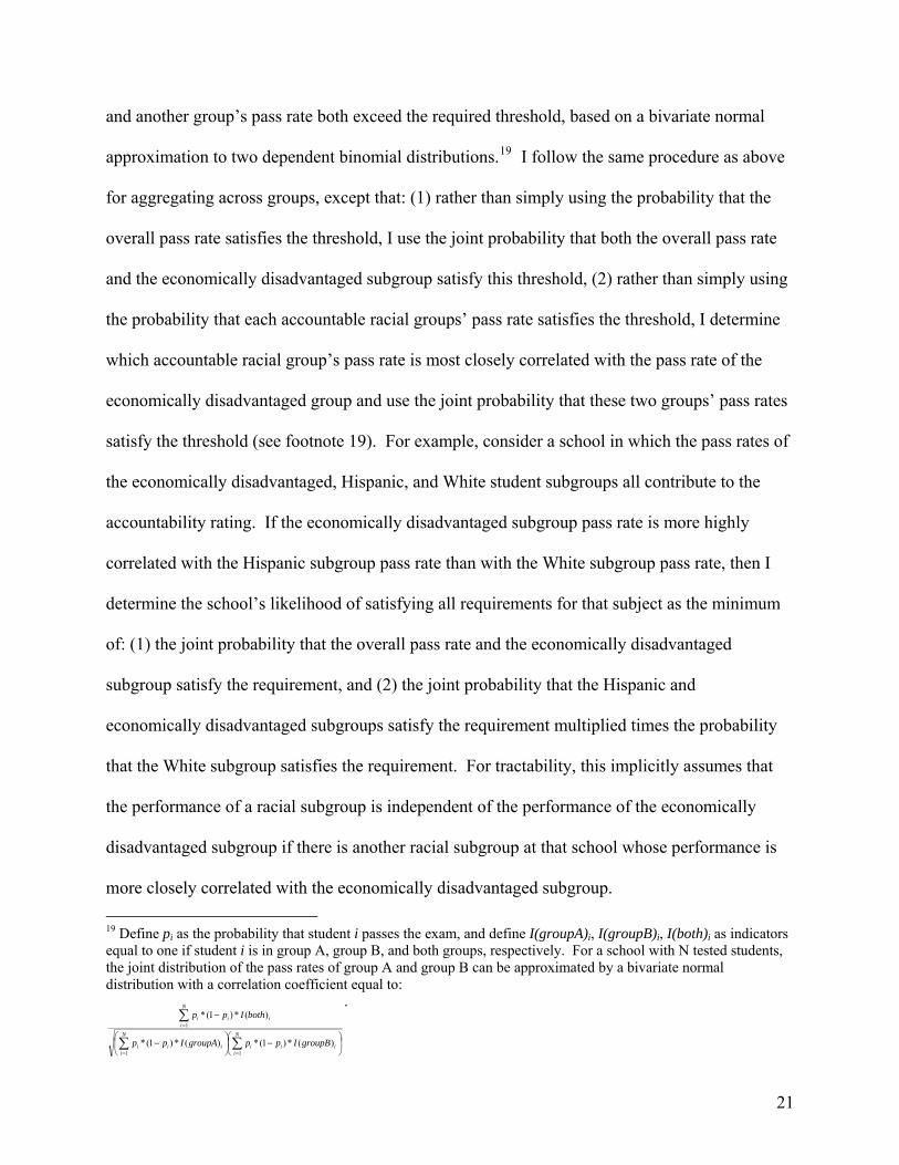
and another group’s pass rate both exceed the required threshold, based on a bivariate normal

approximation to two dependent binomial distributions.19 I follow the same procedure as above

for aggregating across groups, except that: (1) rather than simply using the probability that the

overall pass rate satisfies the threshold, I use the joint probability that both the overall pass rate

and the economically disadvantaged subgroup satisfy this threshold, (2) rather than simply usi

the probability that each accountable racial groups’ pass rate satisfies the threshold, I determine

which accountable racial group’s pass rate is most closely correlated with the pass rate of the

economically disadvantaged group and use the joint probability that these two groups’ pass ra

satisfy the threshold (see footnote 19). For example, consider a school in which the pass rate

the economically disadvantaged, Hispanic, and White student subgroups all contribute to the

accountability rating. If the economically disadvantaged subgroup pass rate is more highly

correlated with the Hispanic subgroup pass rate than with the White subgroup pass rate, th

determine the school’s likelihood of satisfying all requirements for that subject as the

of: (1) the joint probability that the overall pass rate and the economically disadvantaged

subgroup satisfy the requirement, and (2) the joint probability that the Hispanic and

economically disadvantaged subgroups satisfy the requirement multiplied times the probabili

that the White subgroup satisfies the requirement. For tractability, this implicitly assumes that

the performance of a racial subgroup is independent of the performance o

ng

tes

s of

en I

minimum

ty

f the economically

disadva mance is ntaged subgroup if there is another racial subgroup at that school whose perfor

more closely correlated with the economically disadvantaged subgroup. 19 Define pi as the probability that student i passes the exam, and define I(groupA)i, I(groupB)i, I(both)i as indicators equal to one if student i is in group A, group B, and both groups, respectively. For a school with N tested students, the joint distribution of the pass rates of group A and group B can be approximated by a bivariate normal distribution with a correlation coefficient equal to:

⎟⎠

⎞⎜⎝

⎛−⎟

⎠

⎞⎜⎝

⎛−

−

∑∑

∑

==

=

i

N

iiii

N

iii

i

N

iii

groupBIppgroupAIpp

bothIpp

)(*)1(*)(*)1(*

)(*)1(*

11

1

.

21

Finally, I find the marginal effect of a moderate improvement in the expected

achievement of a particular student on the probability that the school obtains the various rating

There is theoretical ambiguity concerning the magnitude of changes in a student’s expected

performance due to moderate changes in the amount of resources devoted to that student. My

preferred approach is to increase expected student performance in a way that is related to the

actual distribution of achievement for similarly skilled students. In particular, I calculate a new,

hypothetical pass probability by re-estimating the student’s pass probability after assuming that

the student will place at or above the Xth percentile of the current year score distribution among

students in the same grade with identical prior year scores. X is set to 25 in the analyses reporte

below, so that the hypothetical improvement is as if the student is guaranteed to finish in the top

three-quarters of the distribution of students with similar prior scores. This amount was chos

because it represents a significant but realistic increase in expected performance, and the main

results below remain qualitatively similar i

s.

d

en

f instead X equals 10, 50, or other values. The results

are also a

whose prior year math pass rate

at that school. The relationship between reading accountability

similar if one uses an alternative way of estimating a hypothetical improvement in

student’s pass probability, such as assigning the pass probability among students with higher

scores on the test during the prior year.20

Figure 2 displays variation in the math incentive measure based on students’ prior

performance and whether the students are members of a group whose prior year math pass rate

was the lowest of any pass rate in that school. Within the same school during the same year, the

incentive measure is greater for students whose prior year pass rate was close to the cutoff

passing score of 70 and for students who are members of a group

was the lowest of any pass rate

20 For example, I estimated models treating a hypothetical improvement as moving to the pass probability among students who scored eight points higher during the prior year.

22

incentives and prior achievement is similar, but math incentives are displayed here because

reading

sts

cross-sectional variation in the impact of school quality on students of

varying abilities.21 The model controls for the same student-level and grade-level variables

(6)

performance requirements are less likely to be binding.

7. Main Empirical Analyses

7.1 School-by-year Fixed Effect Models Analyzing Student-Specific Incentives

The first main model controls for school-by-year fixed effects, so that the relevant

comparison is which students within a school during a particular year receive the largest boo

in achievement. This interpretation assumes that these fixed effects, along with the control

variables, fully capture

described in section 5 and replaces the school-level variables with school-by-year fixed effects:

stjijttisi

stgi Xf

Y ,,,2,,

1,,, εγββα +++∂

+= ,

where

tjv ,∂

si

tjv ,∂als the marginal change in the probability that school j earns a higher rating

year t, given the hypothetical improvement described earlier for stu

f ,∂ equ in

dent i in subject s. For math

incentives, sif

v

,∂∂

incentives the mean equals .0008 with a .0078 standard deviation.

tj , has a mean value of .0010 with a .0043 standard deviation, and for reading

21 This assumption appears to hold very well, probably due to the inclusion of the control variables interacting students’ lagged ability ranges with lagged peer achievement levels. The results below are robust to alternative specifications which add controls for school-by-prior-ability-range fixed effects. These prior ability ranges are again based on the ranges described in Table 2. When one controls for both school-by-year and school-by-prior-ability-range fixed effects, the results are identified from observations with student-level incentives that are relatively large compared to other students within the school that year and compared to students in the same prior ability range in that school during any year. When school-by-prior-achievement range fixed effects are added to the school-by-year fixed effect model, the estimated coefficient for the math student-level incentive in Table 5 only changes from 1.34 to 1.35, and the reading estimate only changes from .954 to .955. This suggests that the estimates in Table 5 are not driven by permanent, between-school differences in schools’ abilities to disproportionately raise the performance of students in a specific part of the achievement distribution.

23

Table 5 displays estimation results for Equation 6. Within the same school during the

same year, students whose individual performance is relatively important for their schools’ rating

enjoy higher than expected gains in test scores. The achievement gains are non-trivial in

magnitude and are statistically significant. If a hypothetical improvement in a student’s

math performance is associated with a .01 greater improvement in the probability that the sc

attains a higher rating, then this student will, on average, score .013 standard deviations higher in

the math score distribution of students with similar prior year scores. To put the magnitude of

this result in perspective, a one standard deviation increase in this incentive measure is

associated with approximately a .007 standard deviation increase in a student’s place in the

statewide achievement distribution. While that may not seem very large, it is important to keep

in mind that this is a within-school effect from

expected

hool

just one year of schooling. Reading performance

incentives w

coefficient for reading incentives equals .954, which implies that a one standard deviation

ace

While

ithin the school are also connected to students’ reading performance: the estimated

change in reading incentives leads to about a .009 standard deviation increase in a student’s pl

in the statewide achievement distribution.22

si

tjv

,

,∂

whether there are high incentives to improve several students’ achievement. I therefore re-

estimate equation 6 with an infra-marginal incentive measure as additional independent

f∂ captures the marginal incentive to improve student i’s performance holding

other students’ expected performance constant, schools strategic responses may be related to

22 Additional analyses re-estimate equation 6 replacing the continuous incentive measure with a discrete, within-school, within-year measure of accountability incentives: an indicator equal to one if the student-level incentive measure is in the highest 10% of all students in that school that year. These additional analyses confirm that the results in Table 5 are not driven by between-school differences in the variance of the student-level incentive measure. Compared to typical progress, students in the highest 10% of incentive levels within their own school in a particular year score .008 standard deviations better in math and .028 standard deviations better in reading, with both estimates statistically significant at the .001 level.

24

variables. The infra-marginal incentive equals the value of si

tj

fv

,

,

∂∂

conditioned on a three

percentage point increase in all of the expected pass rates in the school. A three percentage point

e

infra-marginal math incentive variable has a mean value of .0013 with a .0049 standard

deviation, and for reading the mean equals .0010 with a .0092 standard deviation.

capture the combined effects of student-subject-specific inputs and general student-specific

increase is roughly one standard deviation above the mean improvement in school-wide pass

rates, so this represents a substantial but plausible improvement over the expected rate.23 Th

The estimated coefficients of the student-level incentive variables in these models will

inputs. In other words, the impact of sif ,∂tjv ,∂

may be to schools’ responsiveness to either ib∂

v∂ or

,sic

v∂

∂ . To analyze whether the estimated effects are likely due to student-specific inputs w

transcend specific subject area performance (bi), an additional specification of equation 6

includes separate student-level incentive measures for each subject (math and reading). If

schools are using general student-level inputs, then this would likely be ass

hich

ociated with a

positive

n

6

al and infra-marginal accountability incentives are related to student

cross-subject effect of incentives. For example, greater incentives to improve a

student’s math score would translate into a higher than expected reading score for that student.

If schools are using subject-specific inputs, then the cross-subject effects may be zero, or eve

negative if inputs into one subject crowd out inputs into the other subject.

Table 6 displays results for the models examining the effects of both marginal and infra-

marginal incentives, as well as the impact of cross-subject incentives. The estimates in Table

reveal that both margin

23 Rather than arbitrarily choosing which particular students have higher expected pass probabilities, I assume that the expected values of these pass rates increase by three percentage points without any change in their variance.

25

achieve

a

ject

ther

to

ct marginal incentive

incentiv

ecific

in the required pass rate standards for various ratings, general upward trends in student

ment gains. In Columns 1 and 3 of Table 6, the coefficients on the marginal incentive

variable decrease slightly compared to Table 5, suggesting that some of the positive effect of the

marginal incentive was due to the positive correlation between marginal incentives and infra-

marginal incentives.

Columns 2 and 4 of Table 6 reveal that cross-subject, student-specific incentives have

negative impact on student achievement. Students perform worse than expected in one sub

when there is a greater incentive for schools to improve those students’ performance in the o

subject. The negative cross-subject effects of student-level incentives are more closely related

infra-marginal incentives than marginal incentives, and the cross-subje

measures’ coefficients would be negative and statistically significant if the infra-marginal

es were omitted. The overall negative effects of cross-subject incentives imply that

schools are using student-specific resources which improve performance in one subject at the

expense of other subjects, (i.e., using cis rather than bi in Equation 2).

7.2 School Fixed Effect Models Analyzing Student-Specific and Subject-Specific Incentives

As described in Section 3, schools may also use resources that are not student-sp

inputs in order to improve their expected rating. Examining the same school across different

years, one can find variation in the schools’ incentives to improve the performance of many

students. These incentives vary for the same school due to exogenous, pre-determined changes

achievement over this time period, and in some cases due to variation in which requirements are

binding for the school. To investigate the importance of these incentives, I estimate a school-

fixed effect model including another independent variable, si

tjv ,

g ,∂

∂, which equals the increase in

the probability of school j obtaining a higher rating if all students improve their expected

26

performance. This variable will be related to th rginal benefit from using resources that are e ma

not student specific,sa∂

progress in school-level pass rates, I calculate

tjv∂ , . So that the levels of improvement are within the range of typical

si

tjv ,

g ,∂

∂ based on all students expecting to place

th

similar if one instead uses the 25th percentile.) Because inputs may have d

above the 10 percentile among students with similar past performance. (The estimates are very

ifferential effects on

nt ifferent abilities, I interact si

tj

gv

,

,

∂

∂stude s of d with the vector of indicator variables for the

(7)

student’s prior year test score range, stiR ,1, − . This modified model is thus:

stjijsi

tj

si

tj vRX

vY ,

,

, εαβββ ++stistgi gf ,,,3,

,1,2,1,,, ∂yi

∂++

∂= − ,

∂

with jα capturing school fixed effects and yiX , capturing the same student-level, grade-level,

and school-level control variables described in section 5. In some specifications, this model also

includes cross-subject incentive measures.

Table 7 displays estimates of the effect of incentives in this school fixed effect model.

Compared to the results presented in Table 5, the estimated effects of student-level incentives a

slightly greater for math achievement and slightly smaller for reading achievement. The impact

of school-level incentives differs depending on the student’s prior achievement level. The lowes

achieving students, (who scored between 30 and 45 on the prior year’s test), are the only ones

earning much higher than expected scores when school-level accountability incentives increase

holding student-level accountability incentives constant. This suggests that the spillover effects

of schools’ broad changes to resources or instruction end up helping very low achieving studen

particularly for incentives and achievement in math. Other students do not benefit from these

re

t

ts,

27

broad responses to short-run math incentives. “Marginal achieving students,” whose prior year

score was slightly below or slightly above the passing cutoff, only make higher than expected

math improvements if their own score is important for their school’s rating. In fact, school-level

incentives have a small, negative effect on these students. The same is true for “higher ach

students,” those whose prior year score wa

ieving

s more than four points above the passing cutoff.

by

er

or small-group

at some Texas schools use prior year test

scores

These achievement trends are consistent with schools responding to short-run math incentives

increasing the amount of instruction of very basic mathematics skills and by targeting the

mathematics progress of certain students.

For reading achievement, greater school-level accountability incentives lead to worse

than expected achievement for all but the lowest achieving students. Incentives to raise pe

performance on the reading exam appear to hurt students who have a moderate to strong

probability of passing the exam, unless their own performance is also critical to the school’s

rating. These achievement patterns suggest that schools respond to reading incentives by

substituting away from general subject inputs in favor of student-subject-specific inputs. Rather

than taking actions like spending more time on all students’ reading development, the schools

probably take actions such as pulling out specific students for individualized

reading instruction. There is anecdotal evidence th

and pre-test results to tell teachers which students to focus on and to strategically select

which students participate in after school tutoring (Beam-Conroy, 2001). 24

7.3 Do Schools Shift Resources Across Grades?

24 There is also qualitative evidence that shifting of resources occurs in response to other types of school accountability programs. In order to raise the performance of low achieving students in North Carolina during the 1990’s, principals reported that they “either had to shift resources away from other groups of students or had to ask teachers to spend additional ‘voluntary’ hours after school or on Saturdays working with these students (Ladd and Zelli, 2002, 516).”

28

In addition to shifting resources across students and subjects within the same classro

schools might shift resources across grade levels in response to accountability incentives. While

the theoretical framework presented earlier focused on incentives within a single classroom, one

can extend this framework to consider students spread across multiple classrooms in multi

grades. In certain grades, there might be a greater fraction of students who are close to the

margin for passing the exam and who are members of student subgroups whose performance is

crucial to the school’s rating. There could thus be a great deal of variation in incen

om,

ple

tives across

grade le

fter

lar

effect

ates.

er

l

vels within the same school during the same year, and this variation could lead to

resource shifting across grades. For example, examining teacher characteristics before and a

the adoption of testing in New York, Boyd et. al. (2005) find that new teachers in the high-stakes

grades possess better observable characteristics than new teachers in other grades.

To test for resource shifting based on grade-level incentives, I use grade-level incentives

calculated in the same fashion as the school-level incentives from Section 7.2, based on the

improvement in the school’s probability of earning a higher rating if all students in that particu

grade have higher expected performance. (Grade-level incentives are used because one cannot

match students to specific classrooms.) Table 8 displays results for school-by-year fixed

models, equation 6 with grade-level incentives interacted with students’ prior achievement range

as additional independent variables. The estimates suggest that variation in incentives across

grades within the same school has similar effects as variation across the same school over time.

If a school has a relatively strong incentive to improve students’ math performance in a

particular grade, then the lowest achieving students in that grade outperform similar schoolm

The other students in that grade, however, perform worse than similar schoolmates in the oth

grades, (unless their own performance is relatively important for the school’s rating). If a schoo

29

has a relatively strong incentive to improve some students’ reading performance in a particular

grade, then other students in this grade perform much worse than similar schoolmates. The

findings are again consistent with schools sacrificing general performance in a classroom to

focus on the performance of particular students. Columns 2 and 4 of Table 8 also suggest

schools may be making even larger sacrifices in term

that

s of student performance in other subjects:

s.

ather he

t

performing students who have little chance of passing the exam

during

cross-subject, grade-level incentives have a negative effect on achievement for all student

R than shifting productive resources towards relatively important grades to improve t

performance of all students in these grades, schools appear to be shifting resources across

students and across subjects within these grades.25

7.4 Do Outcomes Reflect Short-run Incentives More Closely in the Terminal Grades?

Another interesting question is whether schools’ short-run responses appear to be

mitigated by long-run incentives. Due to long-run incentives, a school might not want to shif

resources away from very low

the current year. It may be possible that these students will be able to pass the exam

during the following year. If a student is not in the terminal grade at a school, (i.e., the highest

tested grade), then long-run incentives might reduce the shifting of resources away from the

lowest achieving students.

In grades 5, 6, 7, and 8, the fraction of students in the sample who were in the highest

tested grade of their school was about 13%, 37%, 2%, and 96%, respectively. Table 9 displays

25 There is additional evidence of within-grade spillover effects based on the incentives to improve peers of simabilities. I estimated the impact of a school’s incentive to improve the performance of grade-mates with identical prior year scores, controlling for student-level incentives, school-by-year fixed effects, and the same control variables used in Table 8. The results, not shown here, are similar for math and reading. Students in the “low achieving” group perform worse than normal when the school has a strong incentive to improve the performance ofgrade-mates with identical prior year scores, while students in the “higher achieving” group perform better in the

ilar

nalogous situation. These findings are consistent with a triage story in which student-specific investments are more acost effective for improving the performance of students with moderate pass rate probabilities, but general subject investments are more cost effective for improving the performance of students with high pass rate probabilities.

30

regression results using similar specifications as in Table 7, but adding interaction terms based

on whether students are in the terminal grade.26 As expected, schools are even more respon

to short-run incentives for students in the terminal grades. The impact of student-level math

incentives is almost ten times as large in the terminal grades as in other grades. The impact of

student-level reading incentives is more than 50 percent larger for students in the terminal

grades. Unlike other grades, school-level accountability incentives do not have a negative effect

on the achievement of any type of students in the terminal grades. This remains true even if o

repeats these analyses omitting the student-level incentive variables. Although there was not

much evidence of resource shifting based on grade-level inc

sive

ne

entives, these results are consistent

ype of resource shifting across grades: focusing on students in non-terminal

grades e

tional

f

her schoolmates. For

math pe

with a different t

when overall short-run incentives are low, and focusing on the critical students in th

terminal grades when overall short-run incentives are high.

8. Conclusion

The findings suggest that short-run incentives created by a minimum competency

accountability system affect the distribution of student performance gains. These distribu

effects are partially related to schools’ narrowly tailored attempts to improve the performance o

students’ who are on the margin for passing or failing exams. The relative importance of a

student’s performance in a particular subject within a school has a positive effect on that

student’s test score gains in that subject compared to the gains of his or

rformance, the response to student-level accountability incentives is particularly strong

when students are in the final grade offered by their schools, so that the schools have far less

incentive to worry about low achieving students’ future performance.

26 All of the findings in Table 9 are robust to the inclusion of cross-subject incentives, and they are also robust to the inclusion of grade-level fixed effects, which are probably not necessary given that the dependent variable is already based on deviations from grade-level mean scores.

31

Distributional effects also appear to be related to broad responses to year-to-year change

in schools’ accountability incentives. When a school has a realistic chance of improving its

accountability rating by

s

slightly improving student performance in a particular subject, the

lowest

at

ormance. For

exampl

ility

r

e

e incentives by

targeting resources towards the reading performance of particular students, sacrificing these

performing students make greater than expected test score gains in that subject, even

though these students have a negligible chance of passing the exam. Other students only make

greater than expected gains in this situation if their own performance is particularly important for

their schools’ ratings.

Accountability incentives also influence achievement across subjects and across grades.

A greater incentive to improve the performance of a particular student in math decreases th

student’s performance in reading, and a greater incentive to improve the reading score decreases

a student’s performance in math. Within a school in a given year, distributional effects are

amplified for grades in which there are relatively strong incentives to improve perf

e, for math achievement in the relatively important grades, low achieving students

perform better and relatively high achieving students perform worse than similar schoolmates in

other grades. There is also a positive relationship between short-run, school-level accountab

incentives and the performance of students in the terminal grades of their schools.

Considering these collective findings concerning student achievement, one may infe

how schools shift resources based on short-run incentives. Schools respond to math performanc

incentives both by targeting math resources towards specific students and by making broad

changes which also help very low achieving students. These responses tend to sacrifice the

targeted students’ reading performance and to sacrifice relatively high achieving students’

performance in both math and reading. Schools respond to reading performanc

32

student

of

in a

dents

kills. Schools’ strategic exemptions of some students from

testing

ent-

s’ math performance and sacrificing most other students’ performance in reading.

Finally, schools devote fewer resources towards students in the terminal grades during years

when short-run incentives are low than during years when incentives are high.

The advantage of the estimates in this paper, which are based on comparisons with

typical achievement gains made at each point in the achievement distribution, is that they are

unaffected by variation in the difficulty of exams across time or variation in typical gains across

different parts of the achievement distribution. They are also based directly on the short-run

incentives faced by schools using models which control for either school fixed effects or school-

by-year fixed effects. These estimates may in fact understate the distributional consequences

the minimum competency accountability system, because schools might concentrate on low

performing or marginally performing students after the adoption of the accountability system

permanent fashion, rather than waiting for years in which the incentives are greatest. There

could have been permanent, statewide efforts to focus the curriculum on certain types of stu

or skills, and the estimates here would not pick up these potential regime change effects. In

addition, it is possible that accountability incentives negatively affect the performance of the

numerous students whose scores are so high that their performance on the TAAS is not an

accurate measure of their academic progress. Since the TAAS is inherently a minimum skills

test, a school’s focus on basic skills may cause proficient students to make less progress learning

more complicated knowledge and s

may also cause this paper’s estimates to understate the positive impact of school-level

incentives on the performance of low-achieving students and to overstate the impact of stud

level incentives (see Appendix 2).

33

Whether the finding of non-trivial distributional effects is a positive or negative outcome

of this public policy is entirely subjective. If one of the primary goals is to create a sort of

educational triage, in which students below minimum grade-level skills are pushed up, then the

No Child Left Behind type of accountability system appears to be fairly effective. Furthermore

the results say nothing about the overall impact of this system on performance: it may be a rising

tide that lifts all boats (and lifting some more than others), or it may be a falling tide sinking

boats (and sinking some less than others). The important lesson here is that schools respond to

the specific instructional incentives created by the accountability system. Schools’ respo

include targeting specific students, targeting specific subjects, a

,

all

nses

nd making broad changes which

affect all students. An accountability system should only create disproportionate incentives

concerning student achievement gains if the intention is to help some students more than others

and to boost performance in some subjects by more than others. Otherwise, the optimal

accountability system requires a more even-handed approach.

34

Acknowledgements I thank the University of Michigan Economics Department for providing funds to purchase the data used in this paper, and I am grateful to Julie Cullen for helping me clean these data while working on another research project. I appreciate the helpful suggestions of two anonymous referees. I also appreciate helpful comments on earlier drafts of this paper from Julie Cullen, Jonah Rockoff, Miguel Urquiola, as well as seminar participants at Barnard College, Columbia University, Duke University, Hunter College, Teachers College, Union College, the American Education Finance Association Meetings, and the Society for Labor Economics Meetings. The views expressed in this paper and any errors are solely my own. References Beam-Conroy, Teddi, 2001. Bamboozled by the Texas miracle. Rethinking Schools Online

16(1). Boyd, Donald, Lankford, Hamilton, Loeb, Susanna, Wyckoff, James, 2005. The impact of

assessment and accountability on teacher recruitment and retention: Are there unintended consequences? mimeo, www.teacherpolicyresearch.org.

Carnoy, Martin, Loeb, Susanna, Smith, Tiffany L., 2003. The impact of accountability policies in

Texas high schools. In: Carnoy, Martin, Elmore, Richard, and Siskin, Leslie S. (Eds.), The New Accountability: High Schools and High-Stakes Testing, Routledge Falmer.

Consortium for Policy Research in Education, 2000. Assessment and accountability systems: 50

state profiles. at http://www.cpre.org/Publications/Publications_Accountability.htm. Courty, Pascal, Marschke, Gerald, 2004. An empirical investigation of gaming responses to

explicit performance incentives. Journal of Labor Economics 22 (1), 23-56. Courty, Pascal, Marschke, Gerald, 1997. Measuring government performance: Lessons from a

federal job-training program. American Economic Review 87 (2), 383-388. Chay, Kenneth Y., McEwan, Patrick J., Urquiola, Miguel, 2005. The central role of noise in

evaluating interventions that use test scores to rank schools. American Economic Review 95, 1237-1258.

Cullen, Julie Berry, Reback, Randall, 2006. Tinkering toward accolades: School gaming under a

performance accountability system. In: Gronberg, Timothy J., Jansen, Dennis W. (Eds.), Advances in Applied Microeconomics vol. 14 (Improving School Accountability), Elsevier.

Deere, Donald, Strayer, Wayne, 2001. Putting schools to the test: School accountability,

incentives, and behavior. working paper, Texas A&M University.

35

Education Commission of the States, 2002. Rewards and sanctions for school districts and

schools. compiled by Ziebarth, Todd. http://www.ecs.org/clearinghouse/18/24/1824.htm. Grissmer, David, Flanagan, Ann, 1998. Exploring rapid achievement gains in North Carolina

and Texas. National Education Goals Panel, Washington, D.C.. Figlio, David, 2006. Testing, crime, and punishment. Journal of Public Economics 90, 837-851. Figlio, David, Getzler, Lawrence, 2006. Accountability, ability, and disability: Gaming the

system?” In: Gronberg, Timothy J., Jansen, Dennis W. (Eds.), Advances in Applied Microeconomics vol. 14 (Improving School Accountability), Elsevier.

Figlio, David, Lucas, Maurice E., 2004. What’s in a grade? School report cards and house prices.

American Economic Review 94 (4). Figlio, David, Rouse, Cecilia E., 2005. Do accountability and voucher threats improve low-

performing schools? Journal of Public Economics 90, 239-255. Figlio, David, Winicki, Joshua, 2005. Food for thought? The effects of school accountability

plans on school nutrition. Journal of Public Economics 18, 381-394. Hanushek, Eric., Kain, John F., Rivkin, Steven G., 2004. Disruption versus Tiebout

improvement: The costs and benefits of switching schools.” Journal of Public Economics 88 (9), 1721-1746.

Hanushek, Eric., Kain, John F., Rivkin, Steven G., Branch, Gregory F., 2005. Charter school

quality and parental decision making with school choice,” NBER Working Paper 11252. Hanushek, Eric A., Raymond, Margaret E., 2002. Sorting out accountability systems. In Evers,

Williamson M., Walberg, Herbert J. (Eds.), School Accountability, Hoover Institute Press, Stanford, CA.

Hanushek, Eric A., Raymond, Margaret E., 2005. Does school accountability lead to improved

performance? Journal of Policy Analysis and Management 24 (2), 297-327. Heckman, James J., Heinrich, Carolyn J., Smith, Jeffrey, 2002. The performance of performance

standards. Journal of Human Resources 37 (4), 778-811. Holmes, George M., 2003. On teacher incentives and student achievement. mimeo, East

Carolina University Department of Economics. Jacob, Brian, 2005. Accountability, incentives and behavior: the impact of high-stakes testing in

the Chicago Public Schools. Journal of Public Economics 89 (5-6), 761-796.

36

Jacob, Brian, 2001. Getting tough? The impact of mandatory high school graduation exams on student achievement and dropout rates. Educational Evaluation and Policy Analysis 23 (2), 99-122.

Jacob, Brian, Levitt, Steven, 2003. Rotten apples: An investigation of the prevalence and

predictors of teacher cheating. Quarterly Journal of Economics 118 (3), 843-877. Jacobson, Jonathan E., 1993. Mandatory testing requirements and pupil achievement, Doctoral

Disseration, M.I.T. Department of Economics. Kane, Thomas J., Staiger, Douglas E., 2002. The promise and pitfalls of using imprecise school

accountability measures. Journal of Economic Perspectives 16 (4), 91-114.

Ladd, Helen F., Zelli, Arnaldo, 2002. School-based accountability in North Carolina: The responses of school principals. Educational Administration Quarterly 38 (4), 494-529.

Lavy, Victor, 2002. Evaluating the effect of teachers’ group performance incentives on pupil achievement. Journal of Political Economy 110 (6), 1286-1317.

Peabody, Zanto, Markley, Melanie, 2003. State may lower HISD rating; Almost 3,000 dropouts miscounted, report says. Houston Chronicle, A1, June 14, 2003.

Schemo, Diane J., 2004. Schools, facing tight budgets, leave gifted programs behind. New York Times, A1, March 2, 2004.

37

Figure 1 Mean Campus TAAS Pass Rates

0.5

0.55

0.6

0.65

0.7

0.75

0.8

0.85

0.9

1993 1994 1995 1996 1997 1998 1999

Year

Frac

tion

pass

ing

Mathematics

Reading

Writing

38

Figure 2: Mean Student-level Math Accountability Incentives Controlling for School-Year Fixed

Effects, by Students’ Prior Year Math Scores and whether Students were Members of the Subgroup whose Math Pass Rate was the Lowest in Their School during the Prior Year

-.0

010

.001

acco

unta

bilit

y in

cent

ive

30 70 84Students' Prior Year Score

lowest pass rate subgroup not low est pass rate subgroup

Notes to Figure 2: The accountability incentive measure represents the change in the probability that the school earns a higher rating given a hypothetical improvement in a student’s expected performance. As with the main analyses in the

text, this moderate, hypothetical improvement is based on each student’s new pass probability if the student is guaranteed to finish above the 25th percentile among students with identical prior year scores.

Example of Interpretation: On average, compared to moderately increasing the expected performance of a student with mean accountability incentives within the school that year, a school will be about 0.1% more likely to earn a higher

rating if it instead moderately increases the expected performance of a student whose prior year score was 70 and who was a members of the subgroup whose prior year math pass rate was the lowest of any subject and any accountable

subgroup at that school.

39

Table 1. Key Provisions of the Texas Accountability System

Minimum TAAS Pass Rate Maximum Dropout Rate Minimum Attendance Rate E R A E R A E R A 1994 90.0% 65.0% 25.0% 1.0% 3.5% N/A 94.0% 94.0% N/A

1995 90.0% 70.0% 25.0% 1.0% 3.5% 6.0% 94.0% 94.0% N/A

1996 90.0% 70.0% 30.0% 1.0% 3.5% 6.0% 94.0% 94.0% N/A

1997 90.0% 75.0% 35.0% 1.0% 3.5% 6.0% 94.0% 94.0% N/A

1998 90.0% 80.0% 40.0% 1.0% 3.5% 6.0% 94.0% 94.0% N/A

Notes to Table 1: E, R, and A stand for Exemplary, Recognized, and Acceptable ratings, while schools that fail to meet all of these are rated Low-performing. The values above represent the minimum or maximum fraction of students satisfying the performance criteria in order for the school to earn the rating associated with that column. Schools’ performance indicators were based on: current pass rates on the Spring TAAS exams for tested grades, dropout rates for grades 7-12 from the prior year, and the attendance rate for students in grades 1-12 from the prior year. All students and each separate student group (economically disadvantaged, African American, Hispanic, and White) must satisfy the TAAS pass rate and dropout requirements. The TAAS pass rates are calculated separately for each subject (mathematics, reading, and writing).

The dark shading indicates that there are additional requirements (such as sustained performance or required improvement) that mean a school could achieve the indicated standard and still not obtain the indicated rating.

The light shading indicates that there are alternative provisions (such as required improvement and single group waivers) that mean the minimum standards are not always binding.

40

41

Table 2: Pass Rate Probabilities Based on Prior Year Test Score Range

Previous Year’s Scoring Range

Probability of Passing Math based on Previous

Math Score Range

Probability of Passing Reading based on Previous

Reading Score Range

“Lowest Achieving” 30-44 .073 .149 “Very Low Achieving” 45-54 .177 .263

“Low Achieving” 55-64 .392 .458 “Marginal Achieving” 65-74 .690 .691 “Higher Achieving” 75-84 .923 .888

42

Table 3: Summary Statistics for the Sample Means with Standard Deviations in Parentheses

Model with Math Gains as

the Dependent Variable Model with Reading Gains as the Dependent Variable

# of observations 2,540,921 1,876,317 Ri,t-1 (Prior Year Scoring Ranges)

“Lowest Achieving” (30 to 44) .042 .036 “Very Low Achieving” (45 to 54) .084 .077

“Low Achieving” (55 to 64) .146 .149 “Marginal Achieving” (65 to 74) .255 .259

“Higher Achieving” (75 to 84) .472 .479 Student-level control variables

African American Dummy .172 (.378)

.191 (.393)

Hispanic Dummy .355 (.478)

.398 (.489)

Economically Disadvantaged Dummy .479 (.500)

.541 (.498)

(Econ. Dis.)*(African American) .111 (.315)

.129 (.335)

(Econ. Dis.)*(Hispanic) .260 (.439)

.303 (.460)

One-year lagged Test Score in the Other Subject 76.1 (15.2)

68.2 (14.7)

School-level control variables Prior Year’s Attendance Rate .957

(.013) .956

(.014) Enrollment size 737

(312) 734

(310) Number of Students in the Accountable Grades 617

(356) 613

(354) % of students in the accountable grades who were in the accountable pool during the prior year (not exempted)

.754 (.086)

.749 (.088)

% of students who are African American .172 (.378)

.158 (.215)

% of students who are Hispanic .358 (.312)

.384 (.320)

% of students who are Bilingual .151 (.206)

.103 (.142)

% of students who are Economically Disadvantaged .496 (.264)

.526 (.262)

Peer Achievement Levels: school-level & grade-level Quintile Means of Lagged Performance Available from the author upon request

Table 4: Heterogeneous Achievement Gains based on whether Students’ Groups’ Prior Pass Rate was Moderately Below the Current Year’s Target, Regressions Controlling for School Fixed Effects

(1) (2) (3) (4) (5) (6) (7) (8)

All Schools or Those Moderately Below/Above

Particular Ratings? All Acceptable

Rating Recognized

Rating Exemplary

Rating All All All All

Types of Students Included in

Sample All All All All White African

Amer. Hispanic Econ. Disadvant.

MATH INCENTIVES AND MATH ACHIEVEMENT GAINS Coefficients of TREATi,j,s,t Interacted with Students’ Prior Year Scores Ranges:

30-45 (Lowest Achieving) .020 (.007)

.004 (.007)

-.066 (.071)

.118 (.069)

.024 (.016)

.008 (.012)

-.010 (.010)

.0003 (.008)

46-55 (Very Low Ach.) .034 (.005)

.026 (.005)

.004 (.036)

-.008 (.034)

.026 (.009)

.017 (.010)

.007 (.007)

.028 (.006)

56-64 (Low Achieving) .028 (.004)

.017 (.004)

-.031 (.020)

.040 (.019)

.025 (.006)

.022 (.008)

.005 (.006)

.020 (.005)

65-74 (Marginal Achieving) .020 (.003)

.007 (.003)

.035 (.012)

.055 (.011)

.021 (.004)

.013 (.007)

.001 (.005)

.011 (.004)

75-84 (Higher Achieving) .019 (.002)

-.001 (.003)

.093 (.007)

.058 (.007)

.019 (.003)

.005 (.007)

-.012 (.004)

-.005 (.004)

READING INCENTIVES AND READING ACHIEVEMENT GAINS

30-45 (Lowest Achieving) .007 (.009)

.005 (.010)

-.005 (.041)

.045 (.073)

.040 (.019)

-.011 (.015)

-.002 (.013)

-.001 (.010)

46-55 (Very Low Ach.) -.012 (.006)

.001 (.007)

-.031 (.022)

.077 (.042)

-.015 (.012)

-.038 (.012)

-.002 (.009)

-.020 (.007)

56-64 (Low Achieving) -.002 (.004)

.010 (.005)

-.001 (.014)

.020 (.025)

.010 (.008)

-.014 (.009)

-.009 (.007)

-.004 (.006)

65-74 (Marginal Achieving) .009 (.003)

.025 (.004)

.043 (.009)

.062 (.018)

.015 (.006)

.003 (.008)

.006 (.005)

.002 (.005)

75-84 (Higher Achieving) -.001 (.003)

-.002 (.004)

.058 (.007)

.058 (.015)

.012 (.004)

-.012 (.007)

-.012 (.005)

-.012 (.004)

Notes to Table 4: Each column displays estimated coefficients from two regressions, (one for each subject), based on equation 5, a student-level regression model controlling for school fixed effects and student-level race and poverty variables. TREATi,j,s,t is an indicator equal to one if student i contributes to a test pass rate with a prior year value lying below the current year requirement and if none of the school’s prior year test pass rates were more than five percentage points below this requirement. Robust (Huber-White) standard errors are in parentheses. 43

44

Table 5: The Effect of Marginal Accountability Incentives on Student Achievement Gains, Regressions Controlling for School-by-Year Fixed Effects

MATH READING Point Estimate for Student-level Accountability Incentive Variable, (β in equation 6)

1.341 (0.161)

.954 (.210)

Coefficients of Control Variables

One-year lagged Test Score in the Other Subject “ “ “ Squared “ “ “ Cubed

-.124 (.002)

1.24*10-4

(1.08*10-5)

5.03*10-7

(6.04*10-8)

-.038 (.001)

7.54*10-4

(1.35*10-5)

-3.08*10-6

(8.25*10-8)

Economically Disadvantaged African American Hispanic (Economically Disadv.)*(African American) (Economically Disadv.)*(Hispanic) Observations R-squared

-.124 (.002) -.226 (.003) -.141 (.002) .022

(.004) .066

(.003)

2,539,888 .051

-.155 (.003) -.160 (.003) -.144 (.003) .019

(.004) .033

(.004)

1,875,532 .066

Notes to Table 5: Results represent estimates from equation 6, a student-level regression model controlling for school-by-year fixed effects. The regressions also control for quintile mean prior achievement levels for grade-within-school peers. Robust (Huber-White) Standard errors are in parentheses.

45

Table 6: The Effect of Marginal and Infra-Marginal Accountability Incentives on Student

Achievement Gains, Regressions Controlling for School-by-Year Fixed Effects

Dependent Variable: MATH READING Independent Variable:

(1) (2)

(3) (4)

MATH Marginal Incentive

.989 (.247)

.997 (.248) -.119

(.091)

Infra-Marginal Incentive

.411 (.218)

.487 (.219) -.420

(.071)

READING

Marginal Incentive

-.00003 (.144)

.358 (.336)

.396 (.336)

Infra-Marginal Incentive

-.597 (.114)

.690 (.302)

.764 (.302)

Notes to Table 6: Each column represents regression results from estimating equation 6 with the addition of infra-marginal incentive variables. Columns 2 and 4 also include cross-subject incentives. Each infra-marginal incentive variable is calculated in the same fashion as the marginal incentive variable, except that the infra-marginal incentive is calculated after assuming a 3 percentage point increase in the expected value of all pass rates at the school. Robust (Huber-White) standard errors are in parentheses.

46

Table 7: The Relationship between Achievement Gains and both Student-level and School-level Accountability Incentives, Regressions Controlling for School Fixed Effects

MATH READING

MATH INCENTIVES (1) (2) (3) (4)

Student-level Accountability Incentive 1.546 (.159)

1.72 (.159)

-.569 (.059)

School-level Accountability Incentive ….

*(Lowest Achieving) .201 (.043)

.289 (.041)

.105 (.052)

*(Very Low Achieving) .061 (.024)

.125 (.022)

.062 (.031)

*(Low Achieving) .033 (.016)

.058 (.015)

.017 (.019)

*(Marginal Achieving) -.036 (.011)

-.046 (.010)

-.023 (.014)

*(Higher Achieving) -.017 (.007)

-.026 (.007)

-.011 (.009)

READING INCENTIVES

Student-level Accountability Incentive -.629 (.096)

.567 (.211)

.720 (.211)

School-level Accountability Incentive ….

*(Lowest Achieving) .295 (.063)

.089 (.057)

.071 (.058)

*(Very Low Achieving) .132 (.037)

-.105 (.037)

-.113 (.038)

*(Low Achieving) .042 (.025)

-.200 (.026)

-.203 (.026)

*(Marginal Achieving) .010 (.018)

-.201 (.021)

-.202 (.021)

*(Higher Achieving) -.022 (.013)

-.158 (.015)

-.157 (.015)

Notes to Table 7: Each column presents the results of a student-level regression results based on equation 7, which includes school-level and student-level control variables, as well as school fixed effects. Robust (Huber-White) standard errors are in parentheses.

47

Table 8: Grade-level Accountability Incentives and Student Performance, Regressions Controlling for School-by-Year Fixed Effects

MATH READING

MATH INCENTIVES (1) (2) (3) (4)

Student-level Accountability Incentive 1.489 (.165)

1.569 (.166)

-.516 (.059)

Grade-level Accountability Incentive ….

*(Lowest Achieving) .181 (.106)

.188 (.109)

-.406 (.124)

*(Very Low Achieving) -.039 (.071)

-.004 (.072)

-.523 (.089)

*(Low Achieving) -.043 (.059)

-.011 (.059)

-.558 (.072)

*(Marginal Achieving) -.187 (.052)

-.156 (.053)

-.602 (.065)

*(Higher Achieving) -.129 (.049)

-.089 (.050)

-.592 (.061)

READING INCENTIVES

Student-level Accountability Incentive -.539 (.095)

1.339 (.219)

1.48 (.219)

Grade-level Accountability Incentive ….

*(Lowest Achieving) -.195 (.155)

-1.079 (.150)

-.969 (.154)

*(Very Low Achieving) -.347 (.113)

-1.347 (.122)

-1.204 (.124)

*(Low Achieving) -.325 (.098)

-1.579 (.107)

-1.430 (.108)

*(Marginal Achieving) -.339 (.090)

-1.584 (.100)

-1.429 (.102)

*(Higher Achieving) -.420 (.086)

-1.408 (.097)

-1.251 (.098)

Notes to Table 8: Results are based on student-level regressions controlling for students’ race and poverty status, lagged quintile mean grade-level peer achievement, and school-by-year fixed effects. Robust (Huber-White) standard errors are in parentheses.

48

Table 9: Heterogeneous Effects of Short-run Accountability Incentives on Student Achievement, Based on Whether Students are in the Terminal Grade at Their School

MATH READING Student-level Accountability Incentive .378

(.196) .399

(.273)

Student-level Accountability Incentive*(Terminal Grade) 3.025 (.313)

.234 (.411)

School-level Accountability Incentive *(Lowest Achieving)

.089 (.055)

-.068 (.080)

School-level Accountability Incentive *(Lowest Achieving)*(Terminal Grade)

.248 (.079)

.388 (.111)

School-level Accountability Incentive *(Very Low Achieving)

-.022 (.031)

-.398 (.053)

School-level Accountability Incentive *(Very Low Achieving) *(Terminal Grade)

.181 (.041)

.591 (.070)

School-level Accountability Incentive *(Low Achieving)

-.005 (.020)

-.454 (.035)

School-level Accountability Incentive *(Low Achieving) *(Terminal Grade)

.086 (.026)

.567 (.047)

School-level Accountability Incentive *(Marginal Achieving)

-.056 (.013)

-.415 (.027)

School-level Accountability Incentive *(Marginal Achieving) *(Terminal Grade)

.052 (.018)

.496 (.038)

School-level Accountability Incentive *(Higher Achieving)

-.045 (.009)

-.342 (.019)

School-level Accountability Incentive *(Higher Achieving) *(Terminal Grade)

.076 (.011)

.394 (.025)

Notes to Table 9: Coefficient estimates are based on student-level regressions including the school-level and student-level control variables described in equation 7, as well as school fixed effects. Robust (Huber-White) Standard Errors are in parentheses.

A1

Appendix 1: Using Student-level Test Scores to Estimate the Probability that a School Earns a Particular Rating

For grades 4 though 8, groups are based on students with identical scores in reading or

identical scores in math during the prior year, depending on which subject is the outcome of interest. If students are missing prior year scores for certain subjects, I use the other subject score if available, or else use scores from the following year. Although scores from the following year are positively related to shocks in current year scores, there is not an endogeneity problem in this context, because these predicted scores are used simply to determine the expected school-level pass rates. The student-level regression analyses only include students whose scores are predicted based on prior scores and not future scores.

For grade 10, since students are not tested in grade 9, the groups are based on students with identical scores in grade 8 (two years earlier). For all grades, any remaining missing values for student-level pass probabilities are assigned the mean estimated pass probability for students that year in the same grade at the same school.

For grade 3, since this is the first grade of testing and prior scores are never available, I assign the same pass probability to all students within a school, based on the scores of the previous year’s cohort within that school. Rather than simply using the prior cohort’s pass rate, I adjust the pass probability for upward trends in performance. I find the statewide percentile of third grade students who passed in year t, and then calculate the fraction of students in each school’s third grade that scored at that percentile or better in year t-1. School administrators and teachers likely expect an achievement distribution similar to that of the previous year’s third grade cohort, adjusted for upward trends in achievement.

A2

Appendix 2: The Effects of Sample Selection due to Student Exemptions and Grade Repetition There is evidence that schools engage in various other types of strategic behavior in order to improve their accountability ratings. Hanushek and Raymond (2002) summarize early research evidence concerning these strategic responses. The types of behaviors include classifying students as special education or limited English proficient in order to exempt them from testing (Figlio and Getzler, 2006; Cullen and Reback, 2006), improving the nutritional content of school meals shortly before the test administration (Figlio and Winicki, 2005), and altering disciplinary practices (Figlio, 2006). This appendix analyzes whether the estimated effects in this paper are truly due to changes in school services or instructional practices rather than due to strategic exemptions of certain low performing students from contributing to schools’ pass rates. This is particularly important because of this paper’s finding of positive math achievement effects for the lowest performing students, those who have extremely small probabilities of passing.

To estimate the impact of strategic exemptions and grade repetition, I repeat the analyses from Tables 5 and 7 but include all students in the relevant grades and replace the dependent variable with an indicator for whether the student was newly exempted or an indicator for whether the student was retained. Students who are exempted for the first time or retained in the same grade drop out of the samples in the main analyses, though this will only influence the key coefficients of interest if there is selection based on unobservable characteristics. If anything, exempted students might perform worse than observationally equivalent non-exempted students, so that a high propensity to be exempted suggests that a student who remains in the sample may be better along unobserved dimensions.

These analyses reveal mixed results concerning the potential impact of strategic exemptions or retentions on this paper’s main analyses. First, there is evidence of non-linear effects of the student-level incentive variable on the likelihood of attrition from the sample. Two characteristics make students relatively likely to be exempted or retained: whether they are low-performing students who have no chance of passing and whether they are a member of the lowest performing subgroup. Due to the importance of the former characteristic, students are more likely to be exempted or retained in the same grade if small changes in their expected performance do not affect the school’s probability of earning a higher rating. Due to the importance of the latter characteristic, however, the student-level accountability incentive is associated with a greater likelihood of exemption or retention as this incentive measure increases from moderate levels to high levels. Overall, there is a statistically significant, positive relationship between the likelihood of sample attrition and a single linear term measuring the student-level accountability incentive. This relationship is statistically significant but negative, however, when one uses a nonlinear specification such as the natural logarithm of this accountability incentive. If one uses the corresponding nonlinear specification in this paper’s main analyses, the results remain qualitatively similar to those reported above, with large effect sizes for math and smaller effect sizes for reading. Overall, it appears that strategic exemptions and retentions could possibly explain some, but not all, of the estimated effects of student-level incentives in the main analyses.

Second, controlling for student-level incentives, there is actually a negative relationship between school-level incentives and the likelihood of sample attrition. This negative relationship holds for students in all ranges of prior achievement, and it is substantially larger for the lowest achieving students. During years in which the school has a relatively strong incentive to raise pass rates, new exemptions shift away from the lowest performing students towards the students’ whose performance is most critical. For example, if a school’s lowest pass rate is that of the African American student subgroup, then the school might favor placing a low achieving African American student in special education rather than placing an even lower achieving White student

A3

there. If anything, this implies that this paper’s main findings may understate resource shifting which aids the achievement of students with low initial scores. The presence of strong accountability incentives decreases exemptions among these types of students, so that the remaining accountable pool of students may include low achievers with unobserved, negative characteristics.

In summary, while Cullen and Reback (2006) find that Texas schools are more likely to increase exemption levels when they face higher marginal benefits from additional exemptions, this behavior tends to reduce new exemptions among the lowest-performing students and increase new exemptions among students in the most critical subgroups.