Minimizing the Age of Information in Wireless Networks withStochastic Arrivals

Igor Kadota

Massachusetts Institute of Technology

kadota@mit.edu

Eytan Modiano

Massachusetts Institute of Technology

modiano@mit.edu

ABSTRACTWe consider a wireless network with a base station serving multiple

traffic streams to different destinations. Packets from each stream

arrive to the base station according to a stochastic process and are

enqueued in a separate (per stream) queue. The queueing discipline

controls which packet within each queue is available for transmis-

sion. The base station decides, at every time t, which stream to serve

to the corresponding destination. The goal of scheduling decisions

is to keep the information at the destinations fresh. Information

freshness is captured by the Age of Information (AoI) metric.

In this paper, we derive a lower bound on the AoI performance

achievable by any given network operating under any queueing

discipline. Then, we consider three common queueing disciplines

and develop both an Optimal Stationary Randomized policy and a

Max-Weight policy under each discipline. Our approach allows us

to evaluate the combined impact of the stochastic arrivals, queue-

ing discipline and scheduling policy on AoI. We evaluate the AoI

performance both analytically and using simulations. Numerical

results show that the performance of the Max-Weight policy is close

to the analytical lower bound.

CCS CONCEPTS•Networks→Networkperformancemodeling;Networkper-formance analysis; Packet scheduling.

KEYWORDSAge of Information, Scheduling, Wireless Networks, Optimization

ACM Reference Format:Igor Kadota and Eytan Modiano. 2019. Minimizing the Age of Information

in Wireless Networks with Stochastic Arrivals. In The Twentieth ACM Inter-national Symposium on Mobile Ad Hoc Networking and Computing (Mobihoc’19), July 2–5, 2019, Catania, Italy. ACM, New York, NY, USA, 18 pages.

https://doi.org/10.1145/3323679.3326520

1 INTRODUCTIONTraditionally, networks have been designed to maximize through-

put and minimize packet latency. With the emergence of new types

of networks such as vehicular networks, UAV networks and sensor

Permission to make digital or hard copies of all or part of this work for personal or

classroom use is granted without fee provided that copies are not made or distributed

for profit or commercial advantage and that copies bear this notice and the full citation

on the first page. Copyrights for components of this work owned by others than ACM

must be honored. Abstracting with credit is permitted. To copy otherwise, or republish,

to post on servers or to redistribute to lists, requires prior specific permission and/or a

fee. Request permissions from permissions@acm.org.

Mobihoc ’19, July 2–5, 2019, Catania, Italy© 2019 Association for Computing Machinery.

ACM ISBN 978-1-4503-6764-6/19/07. . . $15.00

https://doi.org/10.1145/3323679.3326520

networks, other performance requirements are increasingly rele-

vant. In particular, the Age of Information (AoI) is a performance

metric that was recently proposed in [26, 27] and has been receiving

attention in the literature [1, 2, 5–7, 12–18, 20–22, 24, 27–31, 33–

37, 39–43] for its application in communication systems that carry

time-sensitive data. The AoI captures how fresh the information isfrom the perspective of the destination.

Consider a system in which packets are time-stamped upon

arrival. Naturally, the higher the time-stamp of a packet, the fresher

its information. Let τD (t) be the time-stamp of the freshest packetreceived by the destination by time t . Then, the AoI is defined as

h(t) := t − τD (t). The AoI measures the time that elapsed since the

generation of the freshest packet received by the destination. The

value of h(t) increases linearly over time while no fresher packet is

received, representing the information getting older. At the moment

a fresher packet is received, the time-stamp at the destination τD (t)is updated and the AoI is reduced.

In this paper, we study a wireless network with a Base Station

(BS) serving multiple traffic streams to different destinations over

unreliable channels, as illustrated in Fig. 1. Packets from each stream

arrive to the BS according to a stochastic process and are enqueued

in a separate (per stream) queue. The queueing discipline controls

which packet within each queue is available for transmission. The

BS decides, at every time t , which stream to serve to the correspond-

ing destination. Our goal is to develop scheduling policies that keep

the information fresh at every destination, i.e. that minimize the

average AoI in the network.

In [22], it was shown that when the BS always has fresh packets

available for transmission, the optimal scheduling policy serves

the stream associated with the largest AoI. This policy is optimal1

for it gives the largest reduction in AoI over all streams. However,

when packet arrivals are random, the BS may not have a fresh

packet available for every stream. Thus, a scheduling policy must

account both for the AoI at the destinations and the time-stamps of

the packets available for transmission in each queue. For example,

consider a simple network with two streams and two destinations.

Assume that at time t , each stream has a single packet in its queue.

The packet from stream 1 was generated 30 msecs ago and the

packet from stream 2 was generated 10 msecs ago. Assume that

the current AoI at destinations 1 and 2 are h1(t) = 50 msecs and

h2(t) = 40 msecs, respectively. A policy that serves the stream

associated with the largest AoI would select stream 1 and yield an

AoI reduction of 50 − 30 = 20 msecs. Alternatively, serving stream

2 would result in a reduction of 40 − 10 = 30 msecs. Hence, to

minimize the average AoI, it is optimal to schedule stream 2. In

this simple example, the optimal scheduling decision was easily

1This policy was shown to minimize the average AoI of symmetric networks, i.e.

networks in which all destinations have identical features.

Mobihoc ’19, July 2–5, 2019, Catania, Italy Igor Kadota and Eytan Modiano

determined. In general, designing a transmission scheduling policy

that keeps information fresh over time is a challenging task that

needs to take into account the packet arrival process, the queueing

discipline, and the conditions of the wireless channels.

In recent years, the problem of minimizing the AoI has been

addressed in a variety of contexts. Queueing Theory is used in [6, 7,

16, 24, 27, 29, 31, 43] for finding the optimal server utilization with

respect to AoI. The authors in [1, 2, 35, 41] consider the problem of

optimizing the times in which packets are generated at the source

in networks with energy-harvesting or maximum update frequency

constraints. Applications of AoI are studied in [3, 9, 23, 25, 26].

Link scheduling optimization with respect to AoI has been recently

considered in [4, 5, 8, 12–15, 18, 20–22, 28, 30, 33, 34, 36–40, 42].

Next, we describe the mentioned related work on link scheduling

optimization.

The authors in [5, 8, 37] studied multi-hop networks, while other

works addressed single-hop networks. Deterministic packet arrivals

were considered in [8, 20–22, 28, 36–40, 42], arbitrary arrivals in

[4, 5, 12, 13, 34] and stochastic arrivals in [14, 15, 18, 30, 33, 39].

Networks with no queueing, i.e. when packets are discarded if

not scheduled immediately upon arrival, were considered in [14,

15], First-In First-Out (FIFO) queues were considered in [12, 13,

18, 39] and other works considered Last-Generated First-Served

queues, which are often equivalent to the simpler Last-In First-Out

(LIFO) queues. Reliable links over which transmissions are always

successful are considered in [4, 5, 8, 12–15, 18, 33, 34, 37, 42] and

other works considered unreliable links.

Most relevant to this paper are [14, 18, 20, 21, 34, 39]. In [39], the

authors consider a network with stochastic packet arrivals, FIFO

queues and link scheduling following a Stationary Randomized

policy. An expression for the AoI in a discrete time G/Ber/1 queue

is derived and used to develop a method of jointly tunning arrival

and service rates of all links in order to minimize AoI. In [34], the

authors develop scheduling policies for multi-server queueng sys-

tems in which streams have synchronized packet arrivals. In [14],

the authors develop scheduling policies based on the Whittle’s In-

dex for networks with stochastic arrivals, no queues and reliable

broadcast channels. The authors in [18] utilize an alternative def-

inition of AoI to develop an Age-Based Max-Weight policy for a

network with stochastic arrivals, FIFO queues and unreliable links.

In [20, 21], the authors consider a network with deterministic ar-

rivals, LIFO queues and unreliable broadcast channels, and develop

three policies: Optimal Stationary Randomized, Whittle’s Index and

Age-Based Max-Weight.

In this paper, we develop a framework for addressing linkscheduling optimization in networks with stochastic packetarrivals and unreliable links operating under three commonqueueing disciplines. Our main contributions include: i) deriving

a lower bound on the AoI performance achievable by any given

network operating under any queueing discipline; ii) developing

both an Optimal Stationary Randomized policy and an Age-Based

Max-Weight policy under three common queueing disciplines; and

iii) evaluating the combined impact of the stochastic arrivals, queue-

ing discipline and scheduling policy on AoI. We show that, contrary

to intuition, the Optimal Stationary Randomized policy for LIFO

queues is insensitive to packet arrival rates. Simulation results show

that the performance of the Age-Based Max-Weight policy for LIFO

queues is close to the analytical lower bound.

This paper generalizes our earlier results in [20, 21]. The main

difference is that in [20, 21] we assume that when the BS selects a

stream, a new packet with fresh information is generated and then

transmitted to the corresponding destination in the same time-slot.

It follows that in [20, 21] the packet delay is always 1 slot and theAoI

is reduced to h(t) = 1 slot after every packet delivery. In contrast, in

this paper, we consider a network in which packets are generated

according to a stochastic process and are enqueued before being

transmitted. This seemingly modest distinction affects the packet

delay and the evolution of AoI over time, which in turn affects the

results and proofs throughout the paper significantly. For example,

consider the analysis of Stationary Randomized policies. Under the

assumptions in [20, 21], the AoI evolution is stochastically renewed

after every packet delivery, since h(t) = 1, and thus the AoI can be

analyzed by directly applying the elementary renewal theorem for

renewal-reward processes. In contrast, in this paper, the evolution

of AoI may be dependent across consecutive inter-delivery intervals

and, thus, the same approach is not applicable. To analyze the AoI,

we obtain the stationary distribution of a two-dimensional Markov

Chain in Proposition 4.

The remainder of this paper is organized as follows. In Sec. 2, we

describe the network model. In Sec. 3 we derive an analytical lower

bound on the AoI minimization problem. In Sec. 4, we develop the

Optimal Stationary Randomized policy for each queueing discipline

and characterize their AoI performance. In Sec. 5, we develop the

Max-Weight policy and obtain performance guarantees in terms of

AoI. In Sec. 6, we provide numerical results. The paper is concluded

in Sec. 7. Due to the space constraint, some of the technical proofs

are provided in the report in [19].

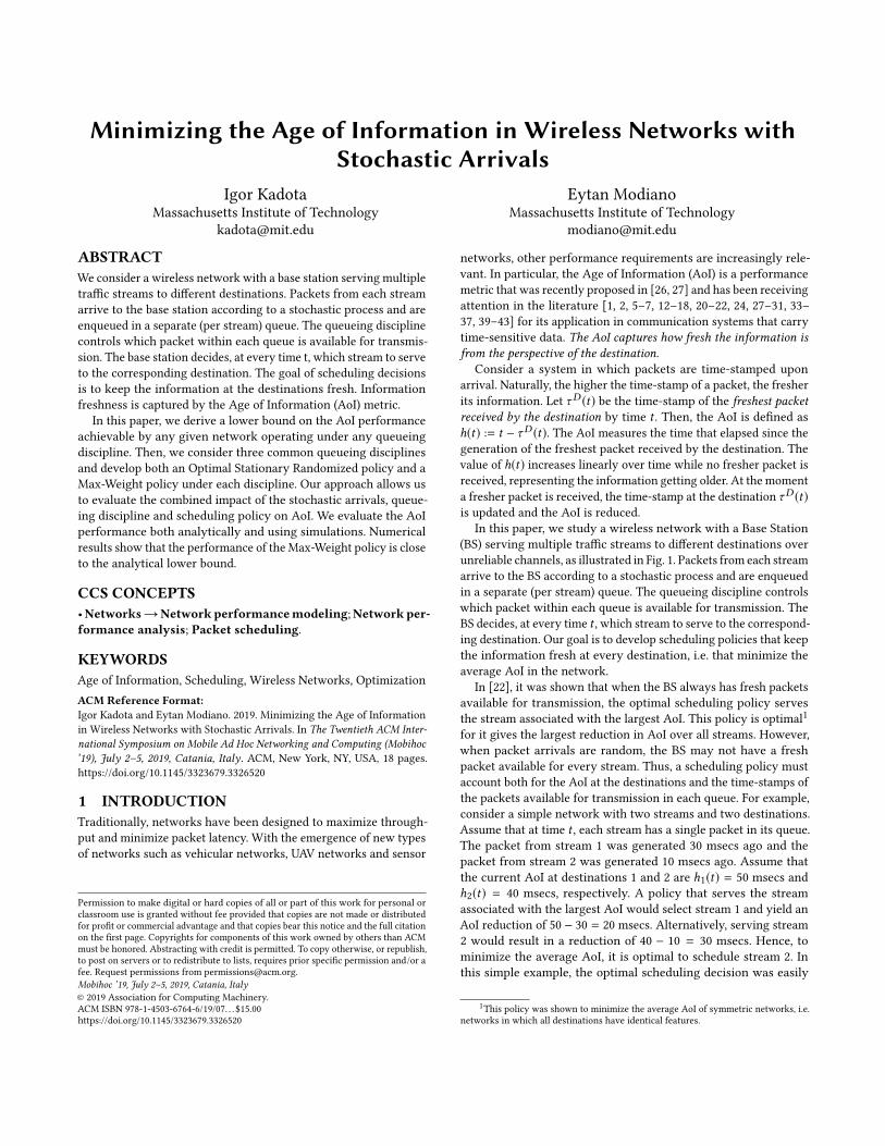
2 SYSTEM MODELConsider a wireless network with a BS serving packets from Nstreams to N destinations, as illustrated in Fig. 1. Time is slotted

with slot index t ∈ 1, 2, · · · ,T , whereT is the time-horizon of this

discrete-time system. At the beginning of every slot t , a new packet

from stream i ∈ 1, 2, · · · ,N arrives to the system with probability

λi ∈ (0, 1],∀i . Let ai (t) ∈ 0, 1 be the indicator function that is

equal to 1when a packet from stream i arrives in slot t , and ai (t) = 0

otherwise. This Bernoulli arrival process is i.i.d. over time and

independent across different streams, with P(ai (t) = 1) = λi ,∀i, t .

Figure 1: Illustration of the wireless network.

Packets from stream i are enqueued in queue i . Denote by Head-

of-Line (HoL) packets the set of packets from all queues that areavailable to the BS for transmission in a given slot t . Depending on

Minimizing the Age of Information in Wireless Networks with Stochastic Arrivals Mobihoc ’19, July 2–5, 2019, Catania, Italy

the queueing discipline employed by the network, queues can be

of three types:

(i) FIFO queues: packets are served in order of arrival. The HoL

packets in slot t are the oldest packets in each queue. This is a

standard queueing discipline, widely deployed in communica-

tion systems. However, only a few works on link scheduling

optimization [12, 13, 18, 39] consider this queueing discipline;

(ii) Single packet queues: when a new packet arrives, older packets

from the same stream are dropped from the queue. The HoL

packets in slot t are the freshest (i.e. most recently generated)

packets in each queue. This queueing discipline is known to

minimize the AoI in a variety of contexts. From the perspectiveof the AoI, Single packet queues are equivalent to LIFO queues;

(iii) No queues: packets can be transmitted only duing the slot in

which they arrive. The HoL packets in slot t are given by the

set i |ai (t) = 1. This queueing discipline is considered in

[14, 15] for its ease of analysis.

Let zi (t) represent the system time of the HoL packet in queue

i at the beginning of slot t . By definition, we have zi (t) := t −τAi (t), where τ

Ai (t) is the arrival time of the HoL packet in queue i .

Naturally, the value of τAi (t) changes only when the HoL packet

changes, namely when the current HoL packet is served or dropped

and there is another packet in the same queue; or when the queue

is empty and a new packet arrives. Notice that zi (t) is undefinedwhen queue i is empty.

We denote by zFi (t), zSi (t) and z

Ni (t), the system times associated

with FIFO queues, Single packet queues and No queues, respectively.For all three cases, whenever the system time is defined, it evolves

according to the definition zi (t) := t − τAi (t). Moreover, it follows

from the description of the queueing disciplines that the evolution

of zSi (t) can be written as

zSi (t) =

0 if ai (t) = 1;

zSi (t − 1) + 1 otherwise,

(1)

and the evolution of zNi (t) is such that zNi (t) = 0 whenever an

arrival occurs, i.e. ai (t) = 1, and is undefined otherwise. In contrast,

the evolution of zFi (t) cannot be simplified for it depends on both

the arrival times and service times of packets in the queue.

In each slot t , the BS either idles or selects a stream and transmits

its HoL packet to the corresponding destination over the wireless

channel. Let ui (t) ∈ 0, 1 be the indicator function that is equal to

1 when the BS transmits the HoL packet from stream i during slot

t , and ui (t) = 0 otherwise. The BS can transmit at most one packet

at any given time-slot t . Hence, we have∑Ni=1

ui (t) ≤ 1,∀t . (2)

The transmission scheduling policy governs the sequence of deci-

sions ui (t)Ni=1

of the BS.

Let ci (t) ∈ 0, 1 represent the channel state associated with

destination i during slot t . When the channel is ON, we have ci (t) =1, and when the channel is OFF, we have ci (t) = 0. The channel

state process is i.i.d. over time and independent across different

destinations, with P(ci (t) = 1) = pi ,∀i, t .Let di (t) ∈ 0, 1 be the indicator function that is equal to 1

when destination i successfully receives a packet during slot t , anddi (t) = 0 otherwise. A successful reception occurs when the HoL

packet is transmitted and the associated channel is ON, implying

that di (t) = ci (t)ui (t),∀i, t . Moreover, since the BS does not know

the channel states prior to making scheduling decisions, ui (t) andci (t) are independent, and E[di (t)] = piE[ui (t)],∀i, t .

The transmission scheduling policies considered in this paper are

non-anticipative, i.e. policies that do not use future information in

making scheduling decisions. Let Π be the class of non-anticipative

policies and let π ∈ Π be an arbitrary admissible policy. Our goal is

to develop scheduling policies π that minimize the average AoI in

the network. Next, we formulate the AoI minimization problem.

2.1 Age of InformationThe AoI depicts how old the information is from the perspective of

the destination. Let hi (t) be the AoI associated with destination iat the beginning of slot t . By definition, we have hi (t) := t − τDi (t),

where τDi (t) is the arrival time of the freshest packet delivered to

destination i before slot t . If during slot t destination i receives apacket with system time zi (t) = t − τAi (t) such that τAi (t) > τDi (t),then in the next slot we have hi (t + 1) = zi (t) + 1. Alternatively, if

during slot t destination i does not receive a fresher packet, then the

information gets one slot older, which is represented by hi (t + 1) =

hi (t) + 1. Notice that the three queueing disciplines considered in

this paper select HoL packets with increasing freshness, implying

that τAi (t) > τDi (t) holds2for every received packet. Hence, the

AoI evolves as follows:

hi (t + 1) =

zi (t) + 1 if di (t) = 1;

hi (t) + 1 otherwise,

(3)

for simplicity, andwithout loss of generality, we assume thathi (1) =1 and zi (0) = 0,∀i . Substituting zFi (t), z

Si (t) and z

Ni (t) into (3) we

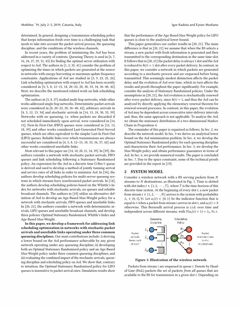
obtain the AoI associated with FIFO queues, Single packet queuesand No queues, respectively. In Fig. 2 we illustrate the evolution of

hi (t) and zi (t) in a network employing Single packet queues.

Figure 2: The blue and orange rectangles represent a packetarrival to queue i and a successful packet delivery to desti-nation i, respectively. The blue curve shows the evolution ofzi (t) for the Single packet queue and the orange curve showsthe AoI associated with destination i.

The time-average AoI associated with destination i is given by

E[∑T

t=1hi (t)

]/T . For capturing the freshness of the information

of a network employing scheduling policy π ∈ Π, we define the

2One example of a queueing discipline that can violate τAi (t ) > τDi (t ) is the Last-

In First-Out (LIFO) queue. When an older packet with τAi (t ) ≤ τDi (t ) is delivered, the

associated AoI does not decrease and the network runs as if no packet was delivered.

It follows that, from the perspective of the AoI, LIFO queues are equivalent to Singlepacket queues.

Mobihoc ’19, July 2–5, 2019, Catania, Italy Igor Kadota and Eytan Modiano

Expected Weighted Sum AoI (EWSAoI) in the limit as the time-

horizon grows to infinity as

E[Jπ

]= lim

T→∞

1

TN

T∑t=1

N∑i=1

wiE[hπi (t)

], (4)

wherewi is a positive real number that represents the priority of

stream i . We denote by AoI-optimal, the scheduling policy π∗ ∈ Πthat achieves minimum EWSAoI, namely

E[J∗] = min

π ∈ΠE

[Jπ

], (5)

where the expectation is with respect to the randomness in the

channel state ci (t), scheduling decisions ui (t) and arrival process

ai (t). Next, we introduce the long-term throughput and discuss the

stability of FIFO queues.

2.2 Long-term ThroughputLet Dπ

i (T ) =∑Tt=1

dπi (t) be the total number of packets delivered

to destination i by the end of the time-horizon T when the admis-

sible policy π ∈ Π is employed. Then, the long-term throughput

associated with destination i is defined as

qπi := lim

T→∞

E [Di (T )]

T. (6)

Throughout this paper, we assume that qπi > 0,∀i . Since packetsfrom stream i are generated at a rate λi , the long-term throughput

provided to destination i cannot be higher than λi . Hence, thelong-term throughput satisfies

qπi ≤ λi ,∀i . (7)

The shared and unreliable wireless channel further restricts the

set of achievable values of long-term throughput qπi Ni=1

. By em-

ploying E[di (t)] = piE[ui (t)] and (2) into the definition of long-

term throughput in (6), we obtain

E[Dπi (T )

]T

=pi

∑Tt=1E[uπi (t)]

T⇒

N∑i=1

qπipi≤ 1 . (8)

Inequalities (7) and (8) are necessary conditions3for the long-

term throughput qπi Ni=1

of any admissible scheduling policy π ∈Π, regardless of the queueing discipline. Both inequalities are used

for deriving the lower bound in Sec. 3. Next, we discuss the stability

of FIFO queues and its impact on the AoI minimization problem.

2.3 Queue StabilityLet Qπ

i (t) be the number of packets in queue i at the beginningof slot t when policy π is employed. Then, we say that queue i isstable if

lim

T→∞E

[Qπi (T )

]< ∞ . (9)

A network is stable under policy π when all of its queues are stable.

For networks with Single packet queues and No queues, stability is

trivial since the backlogs are such thatQπi (t) ∈ 0, 1,∀t , regardless

of the scheduling policy. The discussion about queue stability that

follows is meaningful only for the case of FIFO queues.

3In [20, 30], the authors consider destinations with minimum timely-throughput

requirements. Notice that conditions (7) and (8) are not throughput requirements

enforced by the destinations. They are necessary conditions that follow naturally from

the stochastic arrivals and interference constraints of the network.

Definition 1 (Stability Region). A set of arrival rates λi Ni=1

is within the stability region of a given wireless network if there existsan admissible scheduling policy π ∈ Π that stabilizes all queues.

When the network is unstable under a policy η ∈ Π, then the

expected backlog of at least one of its queues grows indefinitely over

time. An infinitely large backlog leads to packets with infinitely

large system times, i.e. zi (t) → ∞. It follows from the evolution

of hi (t) in (3) that the AoI also increases indefinitely and, as a

result, the Expected Weighted Sum AoI diverges, namely E[Jη ] →∞. Clearly, instability is a critical disadvantage for FIFO queues.Hence, we are interested in scheduling policies that can stabilize the

network whenever the arrival rates λi Ni=1

are within the stability

region. Prior to introducing the policies, we derive a lower bound

to the AoI minimization problem.

3 LOWER BOUNDIn this section, we derive an alternative (and more insightful) ex-

pression for the AoI objective function Jπ in (4) in terms of packet

delay and inter-delivery times. Then, we use this expression to

obtain a lower bound to the AoI minimization problem, namely

LB ≤ E[J∗], for any given network operating under an arbitrary

queueing discipline. Surprisingly, the lower bound LB depends only

on the network’s long-term throughput.

3.1 AoI in terms of packet delay andinter-delivery times

Consider a network employing policy π during the time-horizon

T . Let Ω be the sample space associated with this network and

let ω ∈ Ω be a sample path. For a given sample path ω, let ti [m]be the index of the time-slot in which the mth (fresher

4) packet

was delivered to destination i , ∀m ∈ 1, · · · ,Di (T ), where Di (T )is the total number of packets delivered. Then, we define Ii [m] :=

ti [m] − ti [m − 1] as the inter-delivery time, with Ii [1] = ti [1] andti [0] = 0.

The packet delay associated with the mth packet delivery to

destination i is given by zi (ti [m]). Notice that zi (ti [m]) is the systemtime of the HoL packet at the time it is delivered to the destination,

which is the definition of packet delay. To simplify notation, we

use zi [m] instead of zi (ti [m]).Define the operator

¯M[x] that calculates the sample mean of a

set of values x. Using this operator, the sample mean of Ii [m] for afixed destination i is given by

¯M[Ii ] =1

Di (T )

Di (T )∑m=1

Ii [m] . (10)

For simplicity of notation, the time-horizon T is omitted in the

sample mean operator¯M.

Proposition 2. The infinite-horizon AoI objective function Jπ

can be expressed as follows

Jπ = lim

T→∞

N∑i=1

wi2N

[¯M[I2

i ]

¯M[Ii ]+

2¯M[zi Ii ]¯M[Ii ]

+ 1

]w.p.1 , (11)

4Recall that the delivery of an older packet with τAi (t ) ≤ τ

Di (t ) does not change

the associated AoI and, thus, should not be counted.

Minimizing the Age of Information in Wireless Networks with Stochastic Arrivals Mobihoc ’19, July 2–5, 2019, Catania, Italy

where Ii [m] is the inter-delivery time, zi [m] is the packet delay and

¯M[zi Ii ] =1

Di (T )

Di (T )∑m=1

zi [m − 1]Ii [m] . (12)

Proof. Provided in the technical report [19, Appendix A].

Equation (11) is valid for networks operating under an arbitraryqueueing discipline and employing any scheduling policy π ∈ Π. Asimilar result for the case of a single stream, N = 1, was derived

in [17]. This equation provides useful insights into the AoI mini-

mization. The first term on the RHS of (11), namely¯M[I2

i ]/2¯M[Ii ],

depends only on the service regularity provided by the scheduling

policy. The second term on the RHS of (11) depends on both the

packet delay zi [m − 1] and the inter-delivery time Ii [m], as follows

¯M[zi Ii ]¯M[Ii ]

=

Di (T )∑m=1

Ii [m]∑Di (T )j=1

Ii [j]zi [m − 1] . (13)

Notice that (13) is a weighted sample mean of the packet delays.

Intuitively, for minimizing this term, both the queueing discipline

and the scheduling policy should attempt to deliver packets with

low delay zi [m− 1] and, when the delay is high, they should deliver

the next packet as soon as possible in order to reduce the weight

Ii [m] on the weighted mean (13).

The expression in (11) provides intuition on how the scheduling

policy should manage the packet delays zi [m] and the inter-deliverytimes Ii [m] in order to minimize AoI. Moreover, it shows that by

utilizing the simplifying assumption of queues always having fresh

packets available for transmission, the scheduling policy disregards

zi [m] and fails to address the term in (13). Next, we use (11) to

obtain a lower bound to the AoI minimization problem and, in

upcoming sections, we consider scheduling policies that take into

account both Ii [m] and zi [m].

3.2 Lower BoundA lower bound on AoI is obtained from the expression in Propo-

sition 2. By applying Jensen’s inequality¯M[I2

i ] ≥ (¯M[Ii ])

2to (11),

manipulating the resulting expression and then employing a mini-

mization over policies in Π, we obtain

Lower Bound

LB =min

π ∈Π

1

2N

N∑i=1

wi

(1

qπi+ 1

)(14a)

s.t.

∑Ni=1

qπi /pi ≤ 1 ; (14b)

qπi ≤ λi ,∀i , (14c)

where (14b) and (14c) are the necessary conditions for the long-term

throughput in (8) and (7), respectively. Notice that the optimization

problem in (14a)-(14c) depends only on the network’s long-term

throughput qπi Ni=1

and that the condition qπi ≤ λi limits the

throughput to the packet arrival rate of the respective stream. To

find the unique solution to (14a)-(14c), we analyze the associated

KKT Conditions.

Theorem 3 (Lower bound). For any given network with param-eters (N ,pi , λi ,wi ) and an arbitrary queueing discipline, the opti-mization problem in (14a)-(14c) provides a lower bound on the AoI

minimization problem, namely LB ≤ E[J∗]. The unique solution to(14a)-(14c) is given by

qLBi = min

λi ,

√wipi2Nγ ∗

,∀i , (15)

where γ ∗ yields from Algorithm 1. The lower bound is given by

LB =1

2N

N∑i=1

wi

(1

qLBi

+ 1

). (16)

Algorithm 1 Solution to the Lower Bound

1: γ ← (∑Ni=1

√wi/pi )

2/(2N ) and γi ← wipi/2Nλ2

i ,∀i

2: γ ← maxγ ;γi

3: qi ← λi min1;

√γi/γ ,∀i

4: S ←∑Ni=1

qi/pi5: while S < 1 and γ > 0 do6: decrease γ slightly

7: repeat steps 4 and 5 to update qi and S

8: end while9: return γ ∗ = γ and qLBi = qi ,∀i

Proof. Provided in the technical report [19, Appendix B].

Next, we develop the Optimal Stationary Randomized policy for

different queueing disciplines and derive the closed-form expression

for their AoI performance.

4 STATIONARY RANDOMIZED POLICIESDenote by ΠR the class of Stationary Randomized policies. Let R ∈ΠR be a scheduling policy that, in each slot t , selects stream i withprobability µi ∈ (0, 1] or selects no stream with probability µ0. If

the selected stream i has a non-empty queue, thenui (t) = 1 and the

HoL packet is transmitted by the BS to destination i . Alternatively,if the selected stream i has an empty queue or policy R selected

no stream, then ui (t) = 0,∀i and the BS idles. The scheduling

probabilities µi are fixed over time and satisfy

∑Ni=1

µi = 1 − µ0.

Randomized policies R ∈ ΠR are as simple as possible. Each

policy in ΠR is fully characterized by the set µi Ni=1

. They select

streams at random, without taking into accounthi (t), zi (t) or queuebacklogsQi (t). Notice that policies in ΠR are not work-conserving,

since they allow the BS to idle during slots in which HoL packets

are available for transmission.

Despite their simplicity, we show that by properly tuning thescheduling probabilities µi according to the network parameters

(N ,pi , λi ,wi ), policies in ΠR can achieve performances within a

factor of 4 from the AoI-optimal. On the other hand, we also show

that naive choices of µi can lead to poor AoI performances. Next,

we develop and analyze scheduling policies for different queueing

disciplines which are optimal over the class ΠR . In Secs. 4.1, 4.2

and 4.3 we consider networks employing Single packet queues, Noqueues and FIFO queues, respectively. Then, in Sec. 4.4 we compare

their AoI performances.

Mobihoc ’19, July 2–5, 2019, Catania, Italy Igor Kadota and Eytan Modiano

4.1 Randomized Policy for Single packet queueConsider a network employing the Single packet queue disciplineon N streams with packet arrival rates λi , prioritieswi and channel

reliabilities pi . Recall that for the Single packet queue, when a new

packet arrives, older packets from the same stream are dropped.

The BS selects streams according to R ∈ ΠR with scheduling proba-

bilities µi . Following a successful packet transmission from stream

i , its queue remains empty or a new packet arrives. The expected

number of (consecutive) slots that queue i remains empty is 1/λi −1.

When a new packet arrives, the BS transmits this packet with prob-

ability µi . The expected number of slots necessary to successfully

deliver this packet is 1/pi µi . Under policy R ∈ ΠR and for the case

of Single packet queues, the sequence of packet deliveries is a re-newal process. It follows from the elementary renewal theorem

[10] that

lim

T→∞

1

T

T∑t=1

E[di (t)] =1

1/pi µi + 1/λi − 1

,∀i, t . (17)

For the particular case of λi = 1, the AoI process hi (t) is alsostochastically renewed after every packet delivery and the long-

term time-average E[hi (t)] can be easily obtained using the elemen-

tary renewal theorem for renewal-reward processes. In contrast,

for the general case of λi ∈ (0, 1], the evolution of hi (t) may be

dependent across consecutive inter-delivery intervals due to its

relationship with the system time zSi (t) given in (3). To find an

expression for the long-term time-average E[hi (t)] we formulate

the problem as a two-dimensional Markov Chain with countably-

infinite state space represented by (hi (t), zi (t)) and obtain its sta-

tionary distribution. Proposition 4 follows from substituting the

expression for E[hi (t)] into the objective function in (5).

Proposition 4. The optimal EWSAoI achieved by a network withSingle packet queues over the class ΠR is given by

Optimal Randomized policy for Single packet queues

E[JR

S]= min

R∈ΠR

1

N

N∑i=1

wi

(1

λi− 1 +

1

pi µi

)(18a)

s.t.∑Ni=1

µi ≤ 1 ; (18b)

where RS denotes the Optimal Stationary Randomized Policy for theSingle packet queue discipline.

Proof. Provided in the technical report [19, Appendix C].

Next, we solve the optimization problem in (18a)-(18b) and obtain

the optimal scheduling probabilities µSi Ni=1

.

Theorem 5. Consider a network with parameters (N ,pi , λi ,wi )

operating under the Single packet queues discipline. The optimalscheduling probabilities are given by

µSi =

√wi/pi∑N

j=1

√w j/pj

,∀i , (19)

and the performance of the Optimal Stationary Randomized policyRS is

E[JR

S]=

1

N

N∑i=1

wi

(1

λi− 1

)+

1

N

( N∑i=1

√wipi

)2

. (20)

Then, it follows that

E[J∗

]≤ E

[JR

S]< 4E

[J∗

], (21)

where E [J∗] = minπ ∈Π E [Jπ ] is the minimum AoI over the class of

all admissible policies Π.

Proof. The scheduling probabilities µSi Ni=1

thatminimize (18a)-

(18b) also minimize this equivalent problem

min

R∈ΠR

1

N

N∑i=1

wipi µi

s.t.

N∑i=1

µi ≤ 1 . (22)

Consider the Cauchy–Schwarz inequality( N∑i=1

√wipi

)2

≤

( N∑i=1

µi

) ( N∑i=1

wipi µi

). (23)

The LHS is a lower bound on the objective function in (22). Notice

that Cauchy-Schwarz holds with equality when µSi Ni=1

is given

by (19), implying that (19) is a solution to both (22) and (18a)-(18b).

Substituting the solution5 µSi

Ni=1

into the objective function in

(18a) gives (20).

For deriving the upper bound in (21), consider the Randomized

policy R with µi = qLBi /pi ,∀i . Substitute µi into the RHS of (18a)

and denote the result as E[J R ]. Comparing LB in (16) with E[J R ]

and noting from (15) that qLBi ≤ λi , gives that

E[J R

]≤

1

N

N∑i=1

wi

(2

pi µi− 1

)< 4LB . (24)

By definition, we know that

LB ≤ E[J∗] ≤ E[JR

S] ≤ E[J R ] . (25)

Inequality (21) follows directly from (24) and (25).

Intuitively, the optimal probabilities µiNi=1 should varywith the packet arrival rates λiNi=1. For example, consider a

Single packet queue with low arrival rate and high scheduling prob-

ability. This queue is often offered service while empty, thus wasting

resources. Hence, it seems natural that the optimal µi should vary

with λi . In Secs. 4.2 and 4.3, we show that this is the case for Noqueues and FIFO queues. However, Theorem 5 shows that for Singlepacket queues the optimal µSi depends only onwi and pi. Thisresult is important for it simplifies the design of networkedsystems that attempt to minimize AoI, as discussed in Sec. 4.4.

4.2 Randomized Policy for No queueConsider a network with parameters (N ,pi , λi ,wi ) employing the

No queue discipline and a Stationary Randomized policy R ∈ ΠRwith scheduling probabilities µi . Recall that R is oblivious to packet

arrivals and that, under the No queue discipline, packets are avail-able for transmission only during the slot in which they arrive to

the system. Hence, if R selects stream i during slot t , a success-

ful packet delivery occurs only if a packet from stream i arrivedat the beginning of slot t , i.e. ai (t) = 1, and the channel is ON,

5The expression in (19) was obtained in previous work [21] under the simplifying

assumption of all streams always having fresh packets available for transmission. In

Theorem 5 we show that (19) is in fact optimal for streams with stochastic packet

arrivals and for any set of arrival rates λi Ni=1.

Minimizing the Age of Information in Wireless Networks with Stochastic Arrivals Mobihoc ’19, July 2–5, 2019, Catania, Italy

i.e. ci (t) = 1. Therefore, for the No queue discipline, we have thatdi (t) = ai (t)ci (t)ui (t),∀i, t . This is equivalent to a network with

a virtual channel that is ON with probability piλi and OFF with

probability 1 − piλi . We use this equivalence to derive the results

that follow.

Proposition 6. The optimal EWSAoI achieved by a network withNo queues over the class ΠR is given by

Optimal Randomized policy for No queues

E[JR

N]= min

R∈ΠR

1

N

N∑i=1

wipi µiλi

(26a)

s.t.∑Ni=1

µi ≤ 1 ; (26b)

where RN denotes the Optimal Stationary Randomized policy forthe No queues discipline.

Proof. Under the No queues discipline, all packets are deliveredwith system time zNi (t) = 0 and the AoI process hi (t) is renewedafter every packet delivery. Hence, it follows from the elementary

renewal theorem for renewal-reward processes that

lim

T→∞

1

T

T∑t=1

E[hi (t)] =1

pi µiλi. (27)

Substituting (27) into (5) gives (26a).

Theorem 7. Consider a network with parameters (N ,pi , λi ,wi )

operating under the No queues discipline. The optimal schedulingprobabilities are given by

µNi =

√wi/piλi∑N

j=1

√w j/pjλj

,∀i , (28)

and the performance of the Optimal Stationary Randomized policyRN is

E[JR

N]=

1

N

( N∑i=1

√wipiλi

)2

. (29)

Proof. The proof is similar to Theorem 5.

As expected, the similarities between the Optimal Stationary

Randomized policies for the No queue and Single packet queuedisciplines increase as the packet arrival rates λi

Ni=1

increase.

In particular, notice from (19) and (28) that µNi = µSi ,∀i , whenλi = 1,∀i , and, as a result, their AoI performance is also identical,

namely E[JR

N]= E

[JR

S]when λi = 1,∀i . Recall that µSi does

not change with λi .

4.3 Randomized Policy for FIFO queueConsider a network with parameters (N ,pi , λi ,wi ) employing FIFOqueues and a Stationary Randomized policyR ∈ ΠR with scheduling

probabilities µi . In this setting, each FIFO queue behaves as a discrete-time Ber/Ber/1 queue with arrival rate λi and service rate pi µi . From[11, Sec. 8.10], we know that the FIFO queue is stablewhenpi µi > λiand that its steady-state expected backlog is given by

lim

T→∞E [Qi (T )] =

λi (1 − pi µi )

pi µi − λi. (30)

From [39, Theorem 5]6, we know that the AoI associated with a

stable FIFO queue is given by

lim

T→∞

1

T

T∑t=1

E[hi (t)] =1

pi µi+

1

λi+

[λipi µi

]2

1 − pi µipi µi − λi

. (31)

Notice the similarities between (31), the expected backlog in (30)

and the AoI associated with a Single packet queue in (18a). Under

light load, i.e. when λi << pi µi , the third term on the RHS of (31)

is small when compared to the other terms. Hence, the AoI of the

FIFO queue in (31) is similar to the AoI of the Single packet queuein (18a). On the other hand, under heavy load, as λi → pi µi , thethird term on the RHS of (31) dominates. Both the backlog and

the AoI of the FIFO queue, in (30) and (31), respectively, increase

sharply. Recall that when the backlog is large, packets have to wait

for a long time in the queue before being served, what makes their

information stale and, as a result, the AoI large. The Single packetqueue discipline avoids this issue by keeping only the freshest

packet in the queue.

Denote by RF the Optimal Stationary Randomized policy for the

case of FIFO queues and let µFi Ni=1

be the associated scheduling

probabilities. Substituting (31) into the expression for the EWSAoI

in (5) gives

Optimal Randomized policy for FIFO queues

E[JR

F]= min

R∈ΠR

N∑i=1

wiN

[1

pi µi+

1

λi+

+

[λipi µi

]2

1 − pi µipi µi − λi

](32a)

s.t.

∑Ni=1

µi ≤ 1 ; (32b)

pi µi > λi ,∀i . (32c)

where (32b) is the constraint on scheduling decisions and (32c)

is the condition for network stability.

Remark 8. A sufficient condition for λi Ni=1to be within the

stability region of the network is given by∑Ni=1

λi/pi < 1.

Theorem 9. The optimal scheduling probabilities for the case ofFIFO queues µFi are given by Algorithm 2 when δ → 0.

Proof. The auxiliary parameter δ > 0 is used to enforce a closed

feasible set to the optimization problem in (32a)-(32c). We exchange

(32c) by pi µi ≥ λi + δ ,∀i , to ensure that Algorithm 2 always finds

a unique solution to the KKT Conditions associated with (32a)-

(32c) for any fixed (and arbitrarily small) value of δ . Recall thatwhen pi µi ≈ λi the AoI performance is poor. Hence, in most cases,

the optimal scheduling probabilities µFi Ni=1

are such that pi µFi

and λi are not close, meaning that small changes in δ should not

affect the solution. Algorithm 2 finds the unique solution to the

KKT Conditions and is developed using a similar method as in

Theorem 3.

6The authors in [39] obtain the minimum value of (32a) by jointly optimizing

over scheduling probabilities µFi Ni=1

and packet arrival rates λi Ni=1. Theorem 9

generalizes this result, by providing the optimal µFi Ni=1

for any given λi Ni=1.

Mobihoc ’19, July 2–5, 2019, Catania, Italy Igor Kadota and Eytan Modiano

As part of Algorithm 2, we use the partial derivative of (31) with

respect to µi multiplied bywi/N , which is denoted as

дi (x) =wiN

λi

pi µ2

i

[2

pi µi− 1

]−

pi (1 − λi )

(pi µi − λi )2

x=µi

(33)

Algorithm 2 Randomized policy for FIFO queue

1: γi ← (λi + δ )/pi ,∀i ∈ 1, 2, · · · ,N

2: γ ← maxi −дi (γi ) where дi (.) is given in (33)

3: µi ← max γi ; д−1

i (−γ )

4: S ← µ1 + µ2 + · · · + µN5: while S < 1 do6: decrease γ slightly

7: repeat steps 3 and 4 to update µi and S

8: end while9: return µFi = µi ,∀i

4.4 Comparison of Queueing DisciplinesNext, we compare the performance of four different Stationary

Randomized Policies: 1) Optimal Policy for Single packet queues,RS ; 2) Optimal Policy for No queues, RN ; 3) Optimal Policy for FIFOqueues, RF ; and 4) Naive Policy for FIFO queues. The EWSAoI of

the first three policies is computed using (20), (29) and the solu-

tion to (32a)-(32c), respectively. The Naive Policy shares resources

evenly between streams by assigning µi = 1/N ,∀i . The EWSAoI

of the Naive Policy is computed using the expression inside the

minimization in (32a).

We consider a network with two streams, w1 = w2 = 1, p1 =

1/3, p2 = 1, λ1 = λ, λ2 = λ/3 and varying arrival rates λ ∈0.01, 0.02, · · · , 1. In Fig. 3, we show the EWSAoI of Random-

ized Policies under different queueing disciplines and display the

Lower Bound LB for comparison. The policy with Single packetqueues outperforms the policies with other queueing disciplines for

every arrival rate λ, as expected.

Figure 3: Comparison of Stationary Randomized Policies.

The Optimal Policy for FIFO queues leverages its knowledgeof pi and λi to stabilize the network whenever λi

Ni=1

is within

the stability region. In contrast, the Naive Policy shares channel

resources evenly between streams, disregarding queue stability.

From Remark 8, we know that the network can be stabilized for

λ < 3/10. However, in Fig. 3, we observe that the Naive Policy is

unable to stabilize the network when λ ∈ (1/6, 3/10). By comparing

their performances, it becomes evident that stability is critical for

FIFO queues.Both the Single packet queue and the No queue disciplines present

a natural relationship between the rate at which fresh information

is generated at the source λi and the resulting AoI at the destina-

tion, namely a higher arrival rate (always) leads to a lower AoI.

Furthermore, Theorem 5 shows that the optimal scheduling prob-

abilities µSi for Single packet queues are independent of λi . Thisresult allows us to isolate the design of the arrival rate λifrom the design of the scheduling probability µi. In particular,

to minimize the EWSAoI in the network, the arrival rates λi Ni=1

should be set as high as possible, while the scheduling probabilities

µSi Ni=1

should be proportional to

√wi/pi according to (19). Since

arrival rates and scheduling policies are often defined by dif-ferent layers of the network stack, this isolation simplifiesthe design of networked systems. It is important to empha-size that this isolation only holds for networks employingSingle packet queues. For FIFO queues and No queues the op-timal value of µi changes for different values of λi. Next, wedevelop Age-Based Max-Weight Policies that use the knowledge

of hi (t) and zi (t) for making scheduling decisions in an adaptive

manner.

5 AGE-BASED MAX-WEIGHT POLICIESIn this section, we use Lyapunov Optimization [32] to develop Age-

Based Max-Weight policies for each of the queueing disciplines.

The Max-Weight policy is designed to reduce the expected drift of

the Lyapunov Function at every slot t . In doing so, the Max-Weight

policy attempts to minimize the AoI of the network.

We use the following linear Lyapunov Function

L(hi (t)

Ni=1

)= L(t) =

1

N

N∑i=1

βihi (t) , (34)

where βi is a positive hyperparameter that can be used to tune

the Max-Weight policy to different network configurations and

queueing disciplines. The Lyapunov Drift is defined as

∆(S(t)) := E [L(t + 1) − L(t)| S(t)] , (35)

where S(t) = (hi (t)Ni=1, zi (t)

Ni=1) is the network state at the

beginning of time slot t . The Lyapunov Function L(t) increases withthe AoI of the network and the Lyapunov Drift ∆(S(t)) representsthe expected increase of L(t) in one slot. Hence, by minimizing the

drift in (35) at every slot t , the Max-Weight policy is attempting to

keep both L(t) and the network’s AoI small.

To develop the Max-Weight policy, we analyze the expression

for the drift in (35). Substituting the evolution of hi (t + 1) from (3)

into (35) and then manipulating the resulting expression, we obtain

∆(S(t)) =1

N

N∑i=1

βi −1

N

N∑i=1

βipi (hi (t) − zi (t))E [ui (t)| S(t)] .

(36)

Minimizing the Age of Information in Wireless Networks with Stochastic Arrivals Mobihoc ’19, July 2–5, 2019, Catania, Italy

The scheduling decision in slot t affects only the second term on

the RHS of (36). For minimizing ∆(S(t)), the Max-Weight policyselects, in each slot t , the stream i with a HoL packet and the highestvalue of βipi (hi (t) − zi (t)), with ties being broken arbitrarily. The

Max-Weight policy is work-conserving since it idles only when all

queues are empty.

Substituting zSi (t), zNi (t) and z

Fi (t) into βipi (hi (t) − zi (t)) gives

the Max-Weight policy associated with the Single packet queue,MW S

, the No queue,MW N, and the FIFO queue,MW F

, respectively.

Notice that the difference hi (t) − zi (t) represents the AoI reductionaccrued from a successful packet delivery to destination i . Hence,it makes sense that the Max-Weight policy prioritizes queues with

high potential reward hi (t) − zi (t).

Theorem 10 (Performance Bounds for MW S). Consider a

network employing Single packet queues. The performance of theMax-Weight policy with βi = wi/pi µ

Si ,∀i , is such that

E[JMW S

]≤ E

[JR

S], (37)

where µSi and E[JRS] are the optimal scheduling probability for the

case of Single packet queues and the associated EWSAoI attained byRS , respectively.

Theorem 11 (Performance Bounds for MW N). Consider a

network employing the No queues discipline. The performance of theMax-Weight Policy with βi = wi/pi µ

Ni ,∀i , is such that

E[JMW N

]≤ E

[JR

N], (38)

where µNi and E[JRN] are the optimal scheduling probability for

the case of No queues and the associated EWSAoI attained by RN ,respectively.

The proofs of Theorems 10 and 11 are provided in the technical

report [19, Appendices D and E], respectively. Both proofs rely on

the construction of equivalent systems that facilitate the analysis

of the expression of the drift in (36). The performance ofMW Fis

evaluated next using simulations.

Stationary Randomized policies select streams randomly, accord-

ing to a fixed set of scheduling probabilities µi Ni=1

. In contrast,

Max-Weight policies leverage the knowledge of hi (t) and zi (t) toselect which stream to serve. Therefore, it is not surprising that

Max-Weight policies outperform Randomized policies. However, es-

tablishing a performance guarantee as in (37) and (38) is challenging

for it depends on finding a tight upper bound for the performance

of Max-Weight policies, which often do not have properties such

as renewal intervals that simplify the analysis. Next, we provide

numerical results that further validate the superior performance of

the Max-Weight policies.

6 NUMERICAL RESULTSIn this section, we evaluate the performance of scheduling policies

in terms of the EWSAoI. We compare: i) the Optimal Stationary

Randomized Policy for the case of Single packet queues RS ,No queuesRN and FIFO queues RF ; ii) the Max-Weight Policy

7for the case of

7For the Max-Weight Policies MW S

, MW Nand MW F

, we employ βi =wi /pi µXi , ∀i , where µXi is the optimal scheduling probability for the associated

queueing discipline.

Single packet queuesMW S,No queuesMW N

and FIFO queuesMW F;

and iii) the Whittle’s Index Policy under the No queues discipline.The first two policies were developed in Secs. 4 and 5, respectively,

and the last policy was proposed in [14]. The Lower Bound LBderived in Sec. 3 is displayed for comparison.

In Figs. 4 and 5, we simulate networks with time-horizon T =2 × 10

6slots and N = 4 traffic streams with priorities w1 = 4,

w2 = 4, w3 = 1, w4 = 1, channel reliabilities pi = i/N ,∀i andarrival rates λi = (N − i + 1)/N × λ for λ ∈ 0.01, 0.02, · · · , 0.35.

The results are separated in two figures for clarity. The performance

of the Randomized policies is computed using the expressions in

Sec. 4 while the performance of theMax-Weight andWhittle’s Index

policies are averages over 10 simulation runs.

Figure 4: Simulation of networks with an increasing λ.

Figure 5: Simulation of networks with an increasing λ.

The results in Figs. 4 and 5 suggest that the Max-Weight policy

outperforms the corresponding Randomized and Whittle’s Index

policies with the same queueing discipline for every value of λ. Theresults also show that under the same class of scheduling policies,

Single packet queues outperforms other queueing disciplines for

every value of λ, as expected. It is evident from Fig. 4 that network

instability, which occurs when λ > 12/77, is a major disadvantage

of employing FIFO queues.

Mobihoc ’19, July 2–5, 2019, Catania, Italy Igor Kadota and Eytan Modiano

7 CONCLUDING REMARKSThis paper considers a wireless network with a base station serving

multiple traffic streams to different destinations. Packets from each

stream arrive to the base station according to a Bernoulli process

and are enqueued in separate (per stream) queues that could be of

three types, namely FIFO queue, Single packet queue or No queue,depending on the queueing discipline. Notice that, from the per-

spective of AoI, Single packet queues are equivalent to LIFO queues.

We studied the problem of optimizing scheduling decisions with

respect to the Expected Weighted Sum AoI of the network. Our

main contributions include i) deriving a lower bound on the AoI

performance achievable by any given network operating under

any queueing discipline; ii) developing both an Optimal Stationary

Randomized policy and a Max-Weight policy under each queueing

discipline; and iii) evaluating the combined impact of the stochastic

arrivals, queueing discipline and scheduling policy on the AoI using

analytical and numerical results. We show that, contrary to intu-

ition, the Optimal Stationary Randomized policy for Single packetqueues is insensitive to packet arrival rates. Simulation results show

that the performance of the Age-BasedMax-Weight policy for Singlepacket queues is close to the analytical lower bound. Interesting ex-

tensions of this work include consideration of multi-hop networks

and channels with unknown or time-varying statistics.

8 ACKNOWLEDGMENTThisworkwas supported byNSFGrants AST-1547331, CNS-1713725,

and CNS-1701964, and by Army Research Office (ARO) grant num-

ber W911NF-17-1-0508.

REFERENCES[1] Baran Tan Bacinoglu, Elif Tugce Ceran, and Elif Uysal-Biyikoglu. 2015. Age of

Information under Energy Replenishment Constraints. In Proceedings of IEEEITA.

[2] Baran Tan Bacinoglu and Elif Uysal-Biyikoglu. 2017. Scheduling status updates

to minimize age of information with an energy harvesting sensor. In Proceedingsof IEEE ISIT.

[3] Andrea Baiocchi and Ion Turcanu. 2017. A Model for the Optimization of Bea-

con Message Age-of-Information in a VANET. In 29th International TeletrafficCongress.

[4] Ahmed M. Bedewy, Yin Sun, and Ness B. Shroff. 2016. Optimizing data freshness,

throughput, and delay in multi-server information-update systems. In Proceedingsof IEEE ISIT.

[5] Ahmed M. Bedewy, Yin Sun, and Ness B. Shroff. 2017. Age-Optimal Information

Updates in Multihop Networks. In Proceedings of IEEE ISIT.[6] Kun Chen and Longbo Huang. 2016. Age-of-Information in the Presence of Error.

In Proceedings of IEEE ISIT. 2579–2583.[7] Maice Costa, Marian Codreanu, and Anthony Ephremides. 2016. On the Age of In-

formation in Status Update Systems with Packet Management. IEEE Transactionson Information Theory 62, 4 (2016), 1897–1910.

[8] Shahab Farazi, Andrew G. Klein, John A. McNeill, and D. Richard Brown. 2018.

On the Age of Information in Multi-Source Multi-Hop Wireless Status Update

Networks. In Proceedings of IEEE SPAWC.[9] Antonio Franco, Emma Fitzgerald, Bjorn Landfeldt, Nikolaos Pappas, and Vangelis

Angelakis. 2016. LUPMAC: A Cross-Layer MAC Technique to Improve the Age

of Information Over Dense WLANs. In Proceedings of IEEE ICT.[10] Robert G. Gallager. 2013. Stochastic Processes: Theory for Applications. Cambridge

University Press.

[11] Mor Harchol-Balter. 2013. Performance Modeling and Design of Computer Systems:Queueing Theory in Action. Cambridge University Press.

[12] Qing He, Di Yuan, and Anthony Ephremides. 2016. On Optimal Link Scheduling

with Min-Max Peak Age of Information in Wireless Systems. In Proceedings ofIEEE ICC.

[13] Qing He, Di Yuan, and Anthony Ephremides. 2016. Optimizing Freshness of Infor-

mation: On Minimum Age Link Scheduling in Wireless Systems. In Proceedingsof IEEE WiOpt.

[14] Yu-Pin Hsu. 2018. Age of Information: Whittle Index for Scheduling Stochastic

Arrivals. In Proceedings of IEEE ISIT.[15] Yu-Pin Hsu, Eytan Modiano, and Lingjie Duan. 2017. Age of Information: Design

and Analysis of Optimal Scheduling Algorithms. In Proceedings of IEEE ISIT.[16] Longbo Huang and Eytan Modiano. 2015. Optimizing Age-of-Information in a

Multi-class Queueing System. In Proceedings of IEEE ISIT.[17] Y. Inoue, H.Masuyama, T. Takine, and T. Tanaka. 2017. The stationary distribution

of the age of information in FCFS single-server queues. In Proceedings of IEEEISIT.

[18] Changhee Joo and Atilla Eryilmaz. 2017. Wireless Scheduling for Information

Freshness and Synchrony: Drift-based Design and Heavy-Traffic Analysis. In

Proceedings of IEEE WiOpt.[19] Igor Kadota and Eytan Modiano. 2019. Minimizing the Age of Information

in Wireless Networks with Stochastic Arrivals. Technical Report online:

http://www.igorkadota.com/publications.html.

[20] Igor Kadota, Abhishek Sinha, and Eytan Modiano. 2018. Optimizing Age of

Information in Wireless Networks with Throughput Constraints. In Proceedingsof IEEE INFOCOM.

[21] Igor Kadota, Abhishek Sinha, Elif Uysal-Biyikoglu, Rahul Singh, and Eytan Modi-

ano. 2018. Scheduling Policies for Minimizing Age of Information in Broadcast

Wireless Networks. IEEE/ACM Transactions on Networking (2018).

[22] Igor Kadota, Elif Uysal-Biyikoglu, Rahul Singh, and Eytan Modiano. 2016. Mini-

mizing the Age of Information in Broadcast Wireless Networks. In Proceedings ofIEEE Allerton.

[23] Clement Kam, Sastry Kompella, and Anthony Ephremides. 2015. Experimental

Evaluation of the Age of Information via Emulation. In Proceedings of IEEEMILCOM. 1070–1075.

[24] Clement Kam, Sastry Kompella, Gam D. Nguyen, and Anthony Ephremides. 2016.

Effect of Message Transmission Path Diversity on Status Age. IEEE Transactionson Information Theory 62 (2016), 1360–1374.

[25] Clement Kam, Sastry Kompella, Gam D. Nguyen, Jeffrey E. Wieselthier, and

Anthony Ephremides. 2016. Controlling the age of information: Buffer size,

deadline, and packet replacement. In Proceedings of IEEE MILCOM. 301–306.

[26] Sanjit Kaul, Marco Gruteser, Vinuth Rai, and John Kenney. 2011. Minimizing age

of information in vehicular networks. In Proceedings of IEEE SECON. 350–358.[27] Sanjit Kaul, Roy Yates, and Marco Gruteser. 2012. Real-Time Status: How Often

Should One Update?. In Proceedings of IEEE INFOCOM. 2731–2735.

[28] Sanjit Kaul and Roy D. Yates. 2017. Status Updates over Unreliable Multiaccess

Channels. In Proceedings of IEEE ISIT.[29] Antzela Kosta, Nikolaos Pappas, Anthony Ephremides, and Vangelis Angelakis.

2017. Age and Value of Information: Non-linear Age Case. In Proceedings of IEEEISIT.

[30] Ning Lu, Bo Ji, and Bin Li. 2018. Age-based Scheduling: Improving Data Freshness

for Wireless Real-Time Traffic. In Proceedings of ACM MobiHoc.[31] Elie Najm and Rajai Nasser. 2016. Age of information: The gamma awakening.

In Proceedings of IEEE ISIT. 2574–2578.[32] Michael J. Neely. 2010. Stochastic Network Optimization with Application to

Communication and Queueing Systems. Morgan and Claypool Publishers.

[33] N. Pappas, J. Gunnarsson, L. Kratz, M. Kountouris, and V. Angelakis. 2015. Age

of information of multiple sources with queue management. In Proceedings ofIEEE ICC.

[34] Yin Sun, Elif Uysal-Biyikoglu, and Sastry Kompella. 2018. Age-Optimal Up-

dates of Multiple Information Flows. In IEEE INFOCOM workshop on the Age ofInformation.

[35] Yin Sun, Elif Uysal-Biyikoglu, Roy Yates, C. Emre Koksal, and Ness B. Shroff. 2017.

Update or Wait: How to Keep Your Data Fresh. IEEE Transactions on InformationTheory (2017).

[36] Rajat Talak, Igor Kadota, Sertac Karaman, and Eytan Modiano. 2018. Scheduling

Policies for Age Minimization in Wireless Networks with Unknown Channel

State. In Proceedings of IEEE ISIT.[37] Rajat Talak, Sertac Karaman, and Eytan Modiano. 2017. Minimizing Age-of-

Information in Multi-Hop Wireless Networks. In Proceedings of IEEE Allerton.[38] Rajat Talak, Sertac Karaman, and Eytan Modiano. 2018. Distributed Scheduling

Algorithms for Optimizing Information Freshness in Wireless Networks. In

Proceedings of IEEE SPAWC.[39] Rajat Talak, Sertac Karaman, and Eytan Modiano. 2018. Optimizing Information

Freshness in Wireless Networks under General Interference Constraints. In

Proceedings of ACM MobiHoc.[40] Vishrant Tripathi and Sharayu Moharir. 2017. Age of Information in Multi-Source

Systems. In Proceedings of IEEE Globecom.

[41] Roy D. Yates. 2015. Lazy is Timely: Status Updates by an Energy Harvesting

Source. In Proceedings of IEEE ISIT. 3008–3012.[42] RoyD. Yates, Philippe Ciblat, Aylin Yener, andMicheleWigger. 2017. Age-Optimal

Constrained Cache Updating. In Proceedings of IEEE ISIT.[43] Roy D. Yates and Sanjit Kaul. 2012. Real-time status updating: Multiple sources.

In Proceedings of IEEE ISIT.

Minimizing the Age of Information in Wireless Networks with Stochastic Arrivals Mobihoc ’19, July 2–5, 2019, Catania, Italy

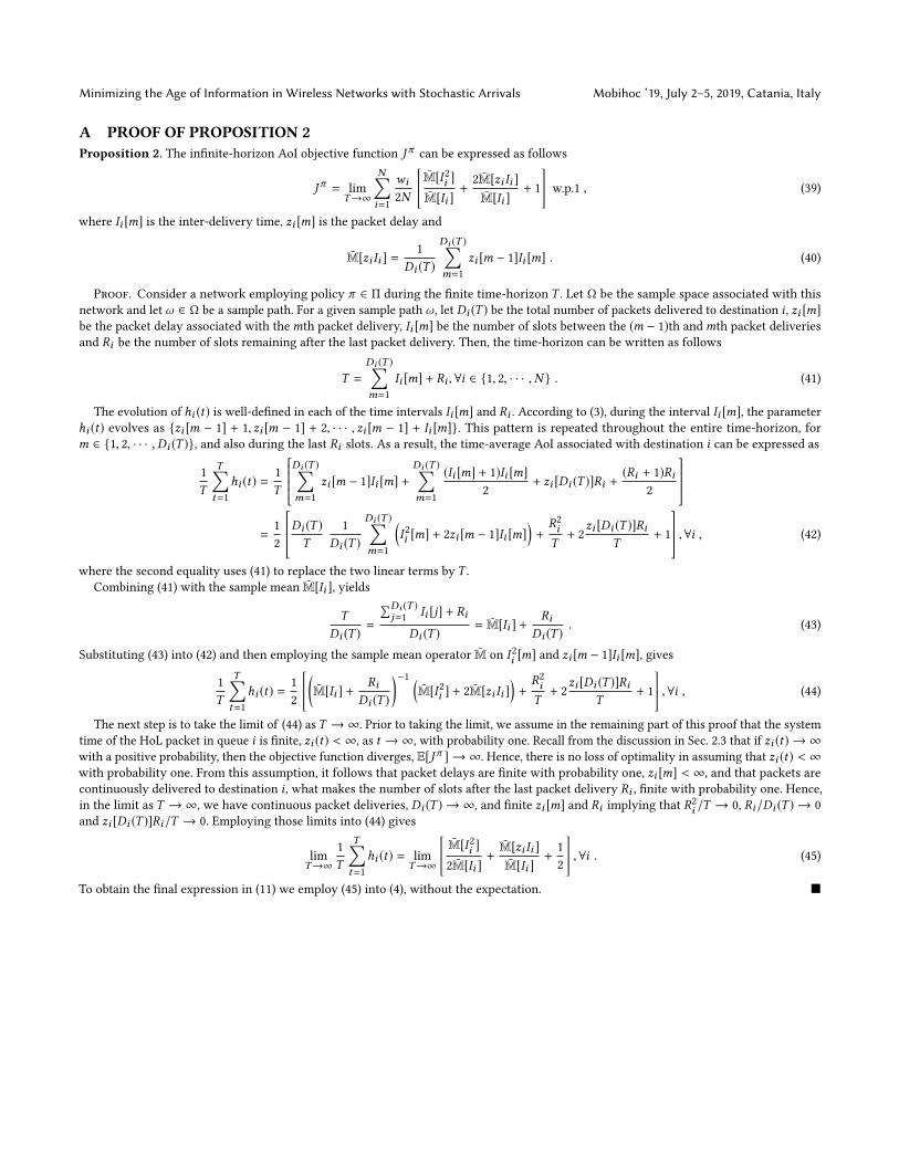
A PROOF OF PROPOSITION 2Proposition 2. The infinite-horizon AoI objective function Jπ can be expressed as follows

Jπ = lim

T→∞

N∑i=1

wi2N

[¯M[I2

i ]

¯M[Ii ]+

2¯M[zi Ii ]¯M[Ii ]

+ 1

]w.p.1 , (39)

where Ii [m] is the inter-delivery time, zi [m] is the packet delay and

¯M[zi Ii ] =1

Di (T )

Di (T )∑m=1

zi [m − 1]Ii [m] . (40)

Proof. Consider a network employing policy π ∈ Π during the finite time-horizon T . Let Ω be the sample space associated with this

network and let ω ∈ Ω be a sample path. For a given sample path ω, let Di (T ) be the total number of packets delivered to destination i , zi [m]be the packet delay associated with themth packet delivery, Ii [m] be the number of slots between the (m − 1)th andmth packet deliveries

and Ri be the number of slots remaining after the last packet delivery. Then, the time-horizon can be written as follows

T =

Di (T )∑m=1

Ii [m] + Ri ,∀i ∈ 1, 2, · · · ,N . (41)

The evolution of hi (t) is well-defined in each of the time intervals Ii [m] and Ri . According to (3), during the interval Ii [m], the parameter

hi (t) evolves as zi [m − 1] + 1, zi [m − 1] + 2, · · · , zi [m − 1] + Ii [m]. This pattern is repeated throughout the entire time-horizon, for

m ∈ 1, 2, · · · ,Di (T ), and also during the last Ri slots. As a result, the time-average AoI associated with destination i can be expressed as

1

T

T∑t=1

hi (t) =1

T

Di (T )∑m=1

zi [m − 1]Ii [m] +

Di (T )∑m=1

(Ii [m] + 1)Ii [m]

2

+ zi [Di (T )]Ri +(Ri + 1)Ri

2

=

1

2

Di (T )

T

1

Di (T )

Di (T )∑m=1

(I2

i [m] + 2zi [m − 1]Ii [m])+R2

iT+ 2

zi [Di (T )]RiT

+ 1

,∀i , (42)

where the second equality uses (41) to replace the two linear terms by T .Combining (41) with the sample mean

¯M[Ii ], yields

T

Di (T )=

∑Di (T )j=1

Ii [j] + Ri

Di (T )= ¯M[Ii ] +

RiDi (T )

. (43)

Substituting (43) into (42) and then employing the sample mean operator¯M on I2

i [m] and zi [m − 1]Ii [m], gives

1

T

T∑t=1

hi (t) =1

2

[(¯M[Ii ] +

RiDi (T )

)−1 (¯M[I2

i ] + 2¯M[zi Ii ]

)+R2

iT+ 2

zi [Di (T )]RiT

+ 1

],∀i , (44)

The next step is to take the limit of (44) asT →∞. Prior to taking the limit, we assume in the remaining part of this proof that the system

time of the HoL packet in queue i is finite, zi (t) < ∞, as t →∞, with probability one. Recall from the discussion in Sec. 2.3 that if zi (t) → ∞with a positive probability, then the objective function diverges, E[Jπ ] → ∞. Hence, there is no loss of optimality in assuming that zi (t) < ∞with probability one. From this assumption, it follows that packet delays are finite with probability one, zi [m] < ∞, and that packets are

continuously delivered to destination i , what makes the number of slots after the last packet delivery Ri , finite with probability one. Hence,

in the limit as T →∞, we have continuous packet deliveries, Di (T ) → ∞, and finite zi [m] and Ri implying that R2

i /T → 0, Ri/Di (T ) → 0

and zi [Di (T )]Ri/T → 0. Employing those limits into (44) gives

lim

T→∞

1

T

T∑t=1

hi (t) = lim

T→∞

[¯M[I2

i ]

2¯M[Ii ]

+¯M[zi Ii ]¯M[Ii ]

+1

2

],∀i . (45)

To obtain the final expression in (11) we employ (45) into (4), without the expectation.

Mobihoc ’19, July 2–5, 2019, Catania, Italy Igor Kadota and Eytan Modiano

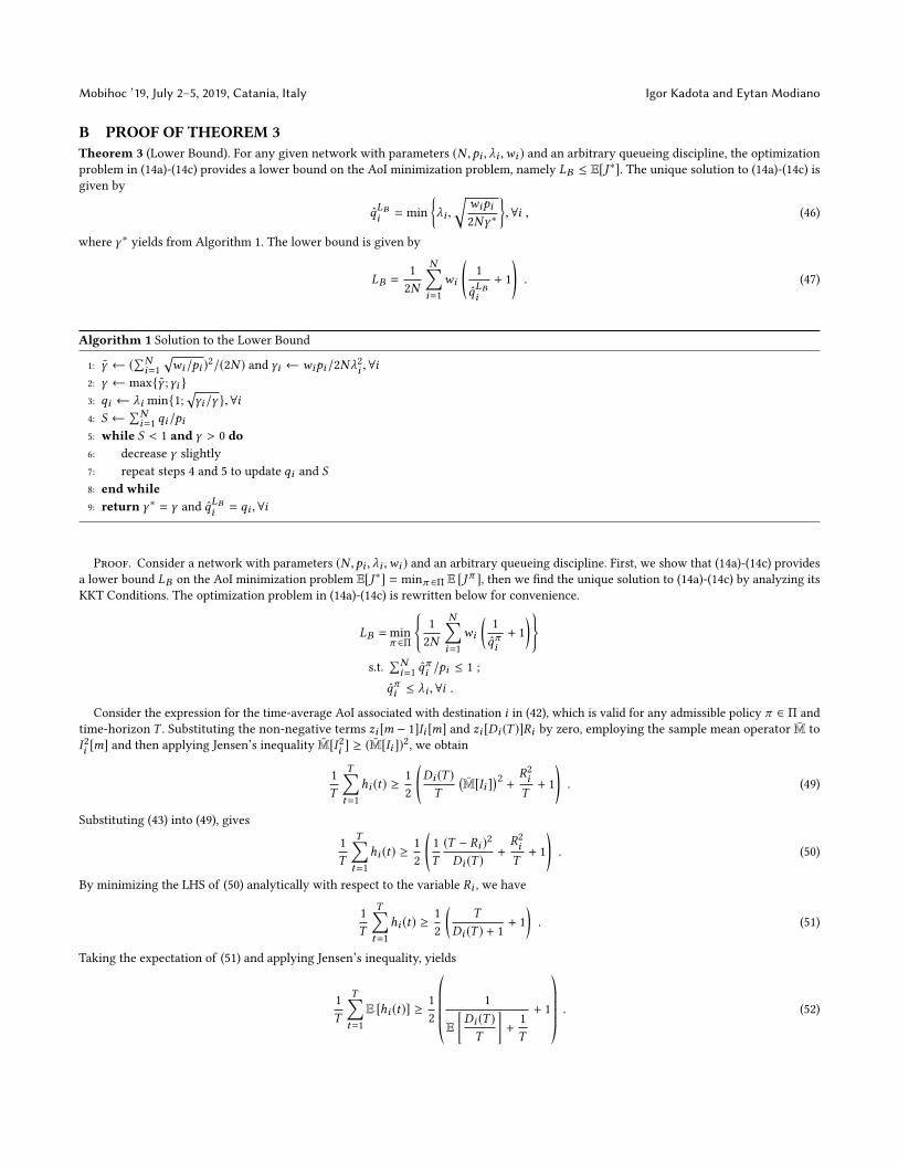
B PROOF OF THEOREM 3Theorem 3 (Lower Bound). For any given network with parameters (N ,pi , λi ,wi ) and an arbitrary queueing discipline, the optimization

problem in (14a)-(14c) provides a lower bound on the AoI minimization problem, namely LB ≤ E[J∗]. The unique solution to (14a)-(14c) is

given by

qLBi = min

λi ,

√wipi2Nγ ∗

,∀i , (46)

where γ ∗ yields from Algorithm 1. The lower bound is given by

LB =1

2N

N∑i=1

wi

(1

qLBi

+ 1

). (47)

Algorithm 1 Solution to the Lower Bound

1: γ ← (∑Ni=1

√wi/pi )

2/(2N ) and γi ← wipi/2Nλ2

i ,∀i

2: γ ← maxγ ;γi

3: qi ← λi min1;

√γi/γ ,∀i

4: S ←∑Ni=1

qi/pi5: while S < 1 and γ > 0 do6: decrease γ slightly

7: repeat steps 4 and 5 to update qi and S

8: end while9: return γ ∗ = γ and qLBi = qi ,∀i

Proof. Consider a network with parameters (N ,pi , λi ,wi ) and an arbitrary queueing discipline. First, we show that (14a)-(14c) provides

a lower bound LB on the AoI minimization problem E[J∗] = minπ ∈Π E [Jπ ], then we find the unique solution to (14a)-(14c) by analyzing its

KKT Conditions. The optimization problem in (14a)-(14c) is rewritten below for convenience.

LB =min

π ∈Π

1

2N

N∑i=1

wi

(1

qπi+ 1

)s.t.

∑Ni=1

qπi /pi ≤ 1 ;

qπi ≤ λi ,∀i .

Consider the expression for the time-average AoI associated with destination i in (42), which is valid for any admissible policy π ∈ Π and

time-horizon T . Substituting the non-negative terms zi [m − 1]Ii [m] and zi [Di (T )]Ri by zero, employing the sample mean operator¯M to

I2

i [m] and then applying Jensen’s inequality¯M[I2

i ] ≥ (¯M[Ii ])

2, we obtain

1

T

T∑t=1

hi (t) ≥1

2

(Di (T )

T

(¯M[Ii ]

)2

+R2

iT+ 1

). (49)

Substituting (43) into (49), gives

1

T

T∑t=1

hi (t) ≥1

2

(1

T

(T − Ri )2

Di (T )+R2

iT+ 1

). (50)

By minimizing the LHS of (50) analytically with respect to the variable Ri , we have

1

T

T∑t=1

hi (t) ≥1

2

(T

Di (T ) + 1

+ 1

). (51)

Taking the expectation of (51) and applying Jensen’s inequality, yields

1

T

T∑t=1

E [hi (t)] ≥1

2

©­­­­«1

E

[Di (T )

T

]+

1

T

+ 1

ª®®®®¬. (52)

Minimizing the Age of Information in Wireless Networks with Stochastic Arrivals Mobihoc ’19, July 2–5, 2019, Catania, Italy

Applying the limit T →∞ to (52) and using the definition of throughput in (6), gives

lim

T→∞

1

T

T∑t=1

E [hi (t)] ≥1

2

(1

qπi+ 1

). (53)

Substituting (53) into the objective function in (4), yields

E[Jπ

]= lim

T→∞

1

N

N∑i=1

wiT

T∑t=1

E [hi (t)]

≥1

2N

N∑i=1

wi

(1

qπi+ 1

). (54)

Inequality (54) is valid for any admissible policy π ∈ Π. Notice that the RHS of (54) depends only on the network’s long-term throughput

qπi Ni=1

. Adding to (54) the two necessary conditions for the long-term throughput in (7) and (8), and then minimizing the resulting problem

over all policies in Π, yields E[J∗] = minπ ∈Π E [Jπ ] ≥ LB where LB is given by (14a)-(14c).

After showing that (14a)-(14c) provides a lower bound on the AoI minimization problem, we find the unique set of network’s long-term

throughput qLBi Ni=1

that solves (14a)-(14c) by analyzing its KKT Conditions. Let γ be the KKT multiplier associated with the relaxation of∑Ni=1

qπi /pi ≤ 1 and ζi Ni=1

be the KKT multipliers associated with the relaxation of qπi ≤ λi ,∀i . Then, for γ ≥ 0 , ζi ≥ 0 and qπi ∈ (0, 1],∀i ,we define

L(qπi ,ζi ,γ ) =1

2N

N∑i=1

wi

(1

qπi+ 1

)+

N∑i=1

ζi(qπi − λi

)+ γ

( N∑i=1

qπipi− 1

), (55)

and, otherwise, we define L(qπi , ζi ,γ ) = +∞. Then, the KKT Conditions are

(i) Stationarity: ∇qπi L(qπi , ζi ,γ ) = 0;

(ii) Complementary Slackness: γ (∑Ni=1

qπi /pi − 1) = 0;

(iii) Complementary Slackness: ζi (qπi − λi ) = 0,∀i;

(iv) Primal Feasibility: qπi ≤ λi ,∀i , and∑Ni=1

qπi /pi ≤ 1;

(v) Dual Feasibility: ζi ≥ 0,∀i , and γ ≥ 0.

Since L(qπi , ζi ,γ ) is a convex function, if there exists a vector (qLBi

Ni=1, ζ ∗i

Ni=1,γ ∗) that satisfies all KKT Conditions, then this vector is

unique. Next, we find the vector (qLBi Ni=1, ζ ∗i

Ni=1,γ ∗).

To assess stationarity, ∇qπi L(qπi , ζi ,γ ) = 0, we calculate the partial derivative of L(qπi , ζi ,γ ) with respect to qπi , which gives

−wipi

2N (qπi )2+ ζipi + γ = 0 ,∀i . (56)

From complementary slackness, γ (∑Ni=1

qπi /pi − 1) = 0, we know that either γ = 0 or

∑Ni=1

qπi /pi = 1. First, we consider the case∑Ni=1

qπi /pi = 1. Based on dual feasibility, ζi ≥ 0, we can separate streams i ∈ 1, · · · ,N into two categories: streams with ζi > 0 and

streams with ζi = 0.

Category 1) stream i with ζi > 0. It follows from complementary slackness, ζi (qπi − λi ) = 0, that qπi = λi . Plugging this value of qπi into (56)

gives the inequality ζipi = γi − γ > 0, where we define the constant

γi :=wipi

2Nλ2

i. (57)

Category 2) stream i with ζi = 0. It follows from (56) that

γ = γi

(λiqπi

)2

⇒ qπi = λi

√γiγ, for γi − γ ≤ 0 . (58)

Hence, for any fixed value of γ ≥ 0, if γ ≥ γi then stream i is in Category 2, otherwise, stream i is in Category 1. Moreover, the values of ζiand qπi associated with stream i , in either Category, can be expressed as

ζi = max

0;

γi − γ

pi

,∀i . (59)

qπi = λi min

1;

√γiγ

,∀i . (60)

Mobihoc ’19, July 2–5, 2019, Catania, Italy Igor Kadota and Eytan Modiano

Notice that when γ > maxγi , then all streams are in Category 2 and qπi < λi ,∀i . By decreasing the value of γ gradually, the throughput

qπi of each stream i in (60) either increases or remain fixed at λi . Our goal is to find the value of γ ∗ which yields qπi Ni=1

satisfying the

condition

∑Ni=1

qπi /pi = 1. Suppose this condition is satisfied when γ > maxγi , with all streams in Category 2, then it follows that

N∑i=1

qπipi=

N∑i=1

λipi

√γiγ=

1√2Nγ

N∑i=1

√wipi= 1⇒

⇒ γ ∗ = γ :=1

2N

( N∑i=1

√wipi

)2

, (61)

where γ is a fixed constant and the solution is unique γ ∗ = γ .

Alternatively, suppose that

∑Ni=1

qπi /pi = 1 is satisfied when minγi ≤ γ ≤ maxγi , with some streams in Category 1 and others in

Category 2. To findγ ∗, we start withγ = maxγi and gradually decreaseγ , adjusting qπi

Ni=1

according to (60) until we reach

∑Ni=1

qπi /pi = 1.

The uniqueness of γ ∗ follows from the monotonicity of qπi with respect to γ in (60).

Another possibility is for γ to reach a value lower than minγi and still result in∑Ni=1

qπi /pi < 1. Notice from (60) that when γ < minγi ,

then all streams are in Category 1 and have maximum throughputs, namely qπi = λi ,∀i . It follows that∑Ni=1

qπi /pi =∑Ni=1

λi/pi < 1, in which

case the condition

∑Ni=1

qπi /pi = 1 cannot be satisfied for any value of γ ≥ 0. Hence, from complementary slackness, γ (∑Ni=1

qπi /pi − 1) = 0,

we have the unique solution γ ∗ = 0.

Proposed algorithm to find γ ∗ that solves the KKT Conditions: start with γ = maxγi ; γ . Then, compute qπi Ni=1

using (60) and verify if

the condition

∑Ni=1

qπi /pi = 1 is satisfied. If

∑Ni=1

qπi /pi < 1, then gradually decrease γ and repeat the procedure. Stop when

∑Ni=1

qπi /pi = 1

or when γ < minγi . If∑Ni=1

qπi /pi = 1 holds, then assign γ ∗ ← γ . Otherwise, if γ < minγi holds, then assign γ ∗ ← 0. The solution to

the KKT Conditions is given by γ ∗ and the associated ζ ∗i and qLBi obtained by substituting γ ∗ into (59) and (60), respectively.

It is evident from the proposed algorithm that for any given network with parameters (N ,pi , λi ,wi ) and an arbitrary queueing discipline,

the solution to the KKT Conditions, (qLBi Ni=1, ζ ∗i

Ni=1,γ ∗), exists and is unique. The proposed algorithm is described using pseudocode in

Algorithm 1.

Minimizing the Age of Information in Wireless Networks with Stochastic Arrivals Mobihoc ’19, July 2–5, 2019, Catania, Italy

C PROOF OF PROPOSITION 4Proposition 4. The optimal EWSAoI achieved by a network with Single packet queues over the class ΠR is given by

Optimal Randomized policy for Single packet queues

E[JR

S]= min

R∈ΠR

1

N

N∑i=1

wi

(1

λi− 1 +

1

pi µi

)(62a)

s.t.

∑Ni=1

µi ≤ 1 ; (62b)

where RS denotes the Optimal Stationary Randomized Policy for the Single packet queue discipline.

Proof. Consider the evolution of hi (t) and zSi (t) given in (3) and (1), respectively. Under policy R ∈ ΠR , the tuple (hi (t), z

Si (t)) evolves

according to a two-dimensional Markov Chain with countably-infinite state space that fully characterizes the state of stream i . The basicstructure of this Markov Chain is illustrated in Fig. 6.

Figure 6: Illustration of the state evolution associated with stream i of a network employing policy R ∈ ΠR and operatingunder the Single packet queue discipline. In partciular, we show the outgoing transition arcs from any given state (hi (t), zi (t)) =(h, z),∀z ∈ 0, 1, 2, · · · ,h ≥ z, with the associated transition probabilities.

To obtain the stationary distribution of stream i’s Markov Chain, we separate its state transitions into three categories and derive the

associated probability distributions.

• Transition to state (h,h),∀h ∈ 1, 2, · · · , following a successful packet transmission and no packet arrival (i.e. transition to an empty8

queue):

P(h,h) = P(1, 0)(1 − λi )

h

λi

1 − (1 − pi µi )

h

pi µi

; (63)

• Transition to state (h, 0),∀h ∈ 1, 2, · · · , following a packet arrival:

P(h, 0) = P(1, 0)

h−1∑n=0

(1 − λi )h−1−n (1 − pi µi )

n

; (64)

• Uneventful transition to state (h, z),∀z ∈ 1, 2, · · · ,h > z:

P(h, z) = P(h − z, 0)(1 − λi )z (1 − pi µi )

z

= P(1, 0)(1 − λi )z (1 − pi µi )

z

h−z−1∑n=0

(1 − λi )h−z−1−n (1 − pi µi )

n

. (65)

Notice that (63), (64) and (65) comprehend all possible state transitions. With the probability distributions, we obtain an expression for the

probability of the event hi (t) = h

P(h) =h∑z=0

P(h, z) =P(1, 0)

λi

[h−1∑n=0

(1 − λi )h−1−n (1 − pi µi )

n

], (66)

for h ≥ 1. Moreover, since

∑h P(h) = 1, we have that P(1, 0) = λ2

ipi µi .

8When the queue is empty, the system time of the HoL packet z is not part of the network state. However, to facilitate the analysis, we assume in this proof that z is always part

of the network state and evolves according to (1).

Mobihoc ’19, July 2–5, 2019, Catania, Italy Igor Kadota and Eytan Modiano

The countable-state Markov Chain is irreducible and has a stationary distribution, hence this distribution is unique, the chain is positive

recurrent and

lim

T→∞

1

T

T∑t=1

E[hi (t)] = E[h] =∑h

hP(h) =1

pi µi+

1

λi− 1 . (67)

Proposition 4 follows from substituting (67) into the objective function in (5).

Minimizing the Age of Information in Wireless Networks with Stochastic Arrivals Mobihoc ’19, July 2–5, 2019, Catania, Italy

D PROOF OF THEOREM 10Theorem 10 (Performance Bounds forMW S

). Consider a network employing Single packet queues. The performance of the Max-Weight

policy with βi = wi/pi µSi ,∀i , is such that

E[JMW S

]≤ E

[JR

S], (68)

where µSi and E[JRS] are the optimal scheduling probability for the case of Single packet queues and the associated EWSAoI attained by RS ,

respectively.

Proof. Consider stream i from a network operating under the Single packet queue discipline. In each slot t , a packet is transmitted, i.e.

ui (t) = 1, if the stream is selected and its queue is non-empty. Hence, packet transmissions ui (t) depend on the queue backlog. To decouple

packet transmissions from the queue backlog, we create dummy packets that can be transmitted without affecting the AoI. In particular,

suppose that at time t queue i is selected and successfully transmits a packet with zSi (t) = z. Then, at the beginning of slot t + 1, with

probability 1 − λi we place a dummy packet with zSi (t + 1) = z + 1 at the HoL of the queue, otherwise we place a real packet with zSi (t) = 0.

From that moment on, the behavior of dummy packets is indistinguishable from real packets. Notice that due to the choice of zSi (t +1) = z+1,

when a dummy packet is delivered to the destination, it does not change the associated AoI. Moreover, the system time zSi (t) is now defined

at every slot t following (1). Next, we analyze the equivalent system with dummy packets.

The Age-Based Max-Weight policy minimizes the drift in (36). Hence, any other policy π ∈ Π yields a higher (or equal) value of ∆(S(t)).Consider the Stationary Randomized policy for Single packet queues defined in Sec. 4.1 with scheduling probability µSi and let

E [ui (t)|S(t)] = E [ui ] = µSi . (69)

Substituting µSi into the Lyapunov Drift gives the upper bound

∆(S(t)) ≤1

N

N∑i=1

βi −1

N

N∑i=1

βipi(hi (t) − z

Si (t)

)µSi . (70)

Now, taking the expectation with respect to S(t) and then the time-average on the interval t ∈ 1, 2, · · · ,T yields

E [L(T + 1)]

T−E [L(1)]

T≤

1

N

N∑i=1

βi −1

TN

T∑t=1

N∑i=1

βipiE[hi (t) − z

Si (t)

]µSi . (71)

Manipulating this expression, assigning βi = wi/pi µSi and taking the limit as T →∞, gives

E[JMW S

]≤

1

N

N∑i=1

wi

pi µSi+ lim

T→∞

1

TN

N∑i=1

T∑t=1

wiE[zSi (t)

]. (72)

From the evolution of zSi (t) in (1), we know that

lim

T→∞

1

TN

N∑i=1

T∑t=1

wiE[zSi (t)

]=

1

N

N∑i=1

wi

(1

λi− 1

). (73)

Substituting (73) into (72) and then comparing the result with (18a) yields

E[JMW S

]≤

1

N

N∑i=1

wi

pi µSi+

1

N

N∑i=1

wi

(1

λi− 1

)= E

[JR

S]. (74)

Mobihoc ’19, July 2–5, 2019, Catania, Italy Igor Kadota and Eytan Modiano

E PROOF OF THEOREM 11Theorem 11 (Performance Bounds forMW N

). Consider a network employing the No queues discipline. The performance of the Max-Weight

Policy with βi = wi/pi µNi ,∀i , is such that

E[JMW N

]≤ E

[JR

N], (75)

where µNi and E[JRN] are the optimal scheduling probability for the case of No queues and the associated EWSAoI attained by RN ,

respectively.

Proof. Consider stream i from a network operating under the No queue discipline. In each slot t , a packet is successfully transmitted, i.e.

di (t) = 1, if a packet arrives, the stream is selected and the channel is ON. Notice that all delivered packets have zNi (t) = 0. This is equivalent

to a network with packets that are always fresh, i.e. zNi (t) = 0,∀i, t , and with a virtual channel that is ON with probability piλi and OFF

with probability 1 − piλi . The Lyapunov Drift for this equivalent system with fresh packets and virtual channels is given by:

∆(S(t)) =1

N

N∑i=1

ˆβi −1

N

N∑i=1

ˆβiλipihi (t)E [ui (t)| S(t)] . (76)

For minimizing ∆(S(t)), the Max-Weight policy selects, in each slot t , the stream i with a HoL packet and the highest value of ˆβiλipihi (t), with

ties being broken arbitrarily. By comparing the drift of the equivalent system (76) and the original system (36), it is easy to see that βi = ˆβiλi .The Age-Based Max-Weight policy minimizes the drift in (76). Hence, any other policy π ∈ Π yields a higher (or equal) value of ∆(S(t)).

Consider the Stationary Randomized policy for No queues defined in Sec. 4.2 with scheduling probability µNi and let

E [ui (t)|S(t)] = E [ui ] = µNi . (77)

Substituting µNi into the Lyapunov Drift gives the upper bound

∆(S(t)) ≤1

N

N∑i=1

ˆβi −1

N

N∑i=1

ˆβiλipihi (t)µNi . (78)

Now, taking the expectation with respect to S(t) and then the time-average on the interval t ∈ 1, 2, · · · ,T yields

E [L(T + 1)]

T−E [L(1)]

T≤

1

N

N∑i=1

ˆβi −1

TN

T∑t=1

N∑i=1

ˆβiλipiE [hi (t)] µNi . (79)

Manipulating this expression, assigningˆβi = wi/λipi µ

Ni and taking the limit as T →∞, gives

E[JMW N

]≤

1

N

N∑i=1

wi

λipi µNi. (80)

For deriving the upper bound in (38), consider the Optimal Stationary Randomized policy RN . Substituting µNi into (26a) and then

comparing with (80) gives

E[JMW N

]≤E

[JR

N]. (81)