minimizemomentsofinertia arXiv:physics/0404005v2 … · 2018-08-27 · 2...

arX

iv:p

hysi

cs/0

4040

05v2

[ph

ysic

s.cl

ass-

ph]

27

Jul 2

005 Using symmetries and generating functions to calculate and

minimize moments of inertia

Rodolfo A. Diaz∗, William J. Herrera†, R. Martinez‡

Universidad Nacional de Colombia,

Departamento de Fısica. Bogota, Colombia.

Abstract

This paper presents some formulae to calculate moments of inertia for solids of revolution and forsolids generated by contour plots. For this, the symmetry properties and the generating functions of thefigures are utilized. The combined use of generating functions and symmetry properties greatly simplifiesmany practical calculations. In addition, the explicit use of generating functions gives the possibility ofwriting the moment of inertia as a functional, which in turn allows to utilize the calculus of variationsto obtain a new insight about some properties of this fundamental quantity. In particular, minimizationof moments of inertia under certain restrictions is possible by using variational methods.

PACS {45.40.-F, 46.05.th, 02.30.Wd}Keywords: Moment of inertia, symmetries, center of mass, generating functions, variational methods.

1 Introduction

The moment of inertia (MI) plays a fundamental role in the mechanics of the rigid rotator [1], and is auseful tool in applied physics and engineering [2]. Hence, its explicit calculation is of greatest interest. Inthe literature, there are alternative methods to facilitate the calculations of MI for beginners [4], at a moreadvanced level [5], or using an experimental approach [6]. Most textbooks in mechanics, engineering andcalculus show some methods to calculate MI’s for certain types of figures [1, 2, 3]. However, they usually donot exploit the symmetry properties of the object to make the calculation easier.

In this paper, we show some quite general formulae in which the MI’s are written in terms of generatingfunctions. On one hand, by combining considerations of symmetry with the generating functions approach,we are able to calculate the MI’s for many solids much easier than using common techniques. On the otherhand, the explicit use of generating functions permits to express the MI’s as functionals; thus, we can usethe methods of the calculus of variations (CV) to study the mathematical properties of the MI for severalkind of figures. In particular, minimization processes of MI’s under certain restrictions are developed byapplying variational methods.

The paper is organized as follows: in Secs. 2, 3 we derive expressions for the MI’s of solids of revolution.In Sec. 4 we calculate MI’s of solids by using the contour plots of the figure, finding formulae for thin platesas a special case. Sec. 5, shows some applications of our formulae, exploring some properties of the MI byusing methods of the CV. Sec. 6, contains the analysis and conclusions.

2 MI’s for solids of revolution generated around the X-axis

2.1 Moment of inertia with respect to the X-axis

Let us evaluate the moment of inertia of a solid of revolution with respect to the axis that generates it,in this case the X−axis according to Fig. 1. We shall assume henceforth, that the solid of revolution is

∗[email protected]†[email protected]‡[email protected]

1

http://arxiv.org/abs/physics/0404005v2

2 Rodolfo A. Diaz, William J. Herrera, R. Martinez

dr

q

y

Z

X

f x2( )

f x1( )

x0

xf

r

r dqdx

drdq

x

x

x

dxx

Y

rx

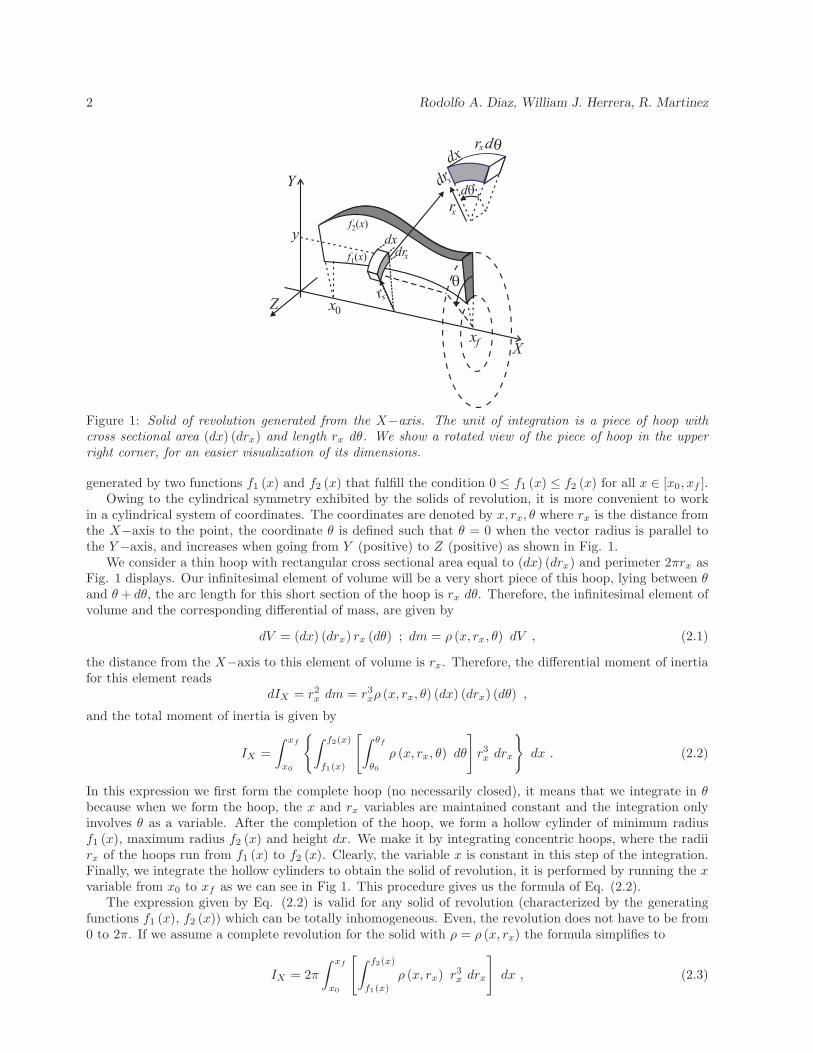
Figure 1: Solid of revolution generated from the X−axis. The unit of integration is a piece of hoop withcross sectional area (dx) (drx) and length rx dθ. We show a rotated view of the piece of hoop in the upperright corner, for an easier visualization of its dimensions.

generated by two functions f1 (x) and f2 (x) that fulfill the condition 0 ≤ f1 (x) ≤ f2 (x) for all x ∈ [x0, xf ].Owing to the cylindrical symmetry exhibited by the solids of revolution, it is more convenient to work

in a cylindrical system of coordinates. The coordinates are denoted by x, rx, θ where rx is the distance fromthe X−axis to the point, the coordinate θ is defined such that θ = 0 when the vector radius is parallel tothe Y−axis, and increases when going from Y (positive) to Z (positive) as shown in Fig. 1.

We consider a thin hoop with rectangular cross sectional area equal to (dx) (drx) and perimeter 2πrx asFig. 1 displays. Our infinitesimal element of volume will be a very short piece of this hoop, lying between θand θ+ dθ, the arc length for this short section of the hoop is rx dθ. Therefore, the infinitesimal element ofvolume and the corresponding differential of mass, are given by

dV = (dx) (drx) rx (dθ) ; dm = ρ (x, rx, θ) dV , (2.1)

the distance from the X−axis to this element of volume is rx. Therefore, the differential moment of inertiafor this element reads

dIX = r2x dm = r3xρ (x, rx, θ) (dx) (drx) (dθ) ,

and the total moment of inertia is given by

IX =

∫ xf

x0

{

∫ f2(x)

f1(x)

[

∫ θf

θ0

ρ (x, rx, θ) dθ

]

r3x drx

}

dx . (2.2)

In this expression we first form the complete hoop (no necessarily closed), it means that we integrate in θbecause when we form the hoop, the x and rx variables are maintained constant and the integration onlyinvolves θ as a variable. After the completion of the hoop, we form a hollow cylinder of minimum radiusf1 (x), maximum radius f2 (x) and height dx. We make it by integrating concentric hoops, where the radiirx of the hoops run from f1 (x) to f2 (x). Clearly, the variable x is constant in this step of the integration.Finally, we integrate the hollow cylinders to obtain the solid of revolution, it is performed by running the xvariable from x0 to xf as we can see in Fig 1. This procedure gives us the formula of Eq. (2.2).

The expression given by Eq. (2.2) is valid for any solid of revolution (characterized by the generatingfunctions f1 (x), f2 (x)) which can be totally inhomogeneous. Even, the revolution does not have to be from0 to 2π. If we assume a complete revolution for the solid with ρ = ρ (x, rx) the formula simplifies to

IX = 2π

∫ xf

x0

[

∫ f2(x)

f1(x)

ρ (x, rx) r3x drx

]

dx , (2.3)

Symmetries and generating functions to calculate moments of inertia 3

and even simpler for ρ = ρ (x)

IX =π

2

∫ xf

x0

ρ (x)[

f2 (x)4 − f1 (x)

4]

dx . (2.4)

We see that all these expressions for the MI of solids of revolution along the axis of symmetry, are writtenin terms of the generating functions f1 (x) and f2 (x). In particular, it follows from Eq. (2.4) that forhomogeneous solids of revolution (and even for inhomogeneous ones whose density depend only on x i.e. theheight of the solid), the volume integral involving the calculation of MI is reduced to a simple integral inone variable. We point out that common textbooks misuse the cylindrical properties of these type of solids,evaluating explicitly all the three integrals even for homogeneous objects.

2.2 Moments of inertia with respect to the Y and Z axes

xZX

r

q

x

Y

rxsinqry

x

ry

Figure 2: Distance from the Y−axis to a differential element of volume. In terms of the coordinates definedin Sec. 2.1 the square distance yields r2y = x2 + r2x sin

2 θ.

Let us calculate the moment of inertia of the solid of revolution with respect to the Y−axis. We use thesame element of volume of the previous section. The square distance from the Y−axis to such element ofvolume is x2 + r2x sin

2 θ, as shown in Fig. 2. Therefore, the moment of inertia of this element of volume withrespect to Y reads

dIY =(

r2x sin2 θ + x2

)

dm ,

with dm given by Eq. (2.1). Integrating in a way similar to the previous section, the MI becomes

IY =

∫ xf

x0

{

∫ f2(x)

f1(x)

[

∫ θf

θ0

ρ (x, rx, θ) sin2 θ dθ

]

r3x drx

}

dx+

+

∫ xf

x0

{

∫ f2(x)

f1(x)

[

∫ θf

θ0

ρ (x, rx, θ) dθ

]

rx drx

}

x2 dx . (2.5)

Once again, this formula is valid for any inhomogeneous solid of revolution (even incomplete) generated bythe functions f1 (x), f2 (x). When assuming a complete solid of revolution with ρ = ρ (x, rx), and takinginto account Eq. (2.3), the latter formula reduces to

IY =1

2IX + 2π

∫ xf

x0

x2

[

∫ f2(x)

f1(x)

ρ (x, rx) rx drx

]

dx . (2.6)

From this expression we derive the interesting property IY ≥ IX/2, which is valid for any complete solid ofrevolution with azimuthal symmetry. Additionally, for ρ = ρ (x) we have

IY =1

2IX + π

∫ xf

x0

ρ (x) x2[

f2 (x)2 − f1 (x)

2]

dx . (2.7)


By the same token, for the Z−axis, which is perpendicular to the X and Y−axes and with the origin asthe intersection point, we have the following general formula

IZ =

∫ xf

x0

{

∫ f2(x)

f1(x)

[

∫ θf

θ0

ρ (x, rx, θ) cos2 θ dθ

]

r3x drx

}

dx+

+

∫ xf

x0

{

∫ f2(x)

f1(x)

[

∫ θf

θ0

ρ (x, rx, θ) dθ

]

rx drx

}

x2 dx . (2.8)

We emphasize that in the case of a complete revolution, the formula (2.8), coincides exactly with IY in Eq.(2.6) when ρ does not depend on θ, as expected from the cylindrical symmetry. Indeed, for IZ to be equalto IY , the requirement of azimuthal symmetry could be softened by demanding the conditions

ρ = ρ (x, rx) ρ (θ) ;

∫ θf

θ0

ρ (θ) sin2 θ dθ =

∫ θf

θ0

ρ (θ) cos2 θ dθ , (2.9)

for if the conditions (2.9) are held, we get that

∫ θf

θ0

ρ (θ) cos2 θ dθ =1

2

∫ θf

θ0

ρ (θ) dθ ,

and IY = IZ even for an incomplete solid of revolution with no azimuthal symmetry.From Eqs. (2.5-2.8), we see that for the calculation of the MI for axes perpendicular to the axis of

symmetry, we use the same limits of integration as for the symmetry axis; thus, we do not have to careabout the partitions. Once again, these MI’s are written in terms of the generating functions of the solidf1 (x) and f2 (x).

Finally, we emphasize that textbooks do not usually report the moments of inertia for solids of revolutionwith respect to axes perpendicular to the axis of symmetry. However, they are important in many physicalproblems. For instance, a solid of revolution acting as a physical pendulum requires the calculation of suchMI’s, see example 8.

h

X

Y

Z

a2

a1

R

H

f1 (x)

f1 (x)

f2 (x)

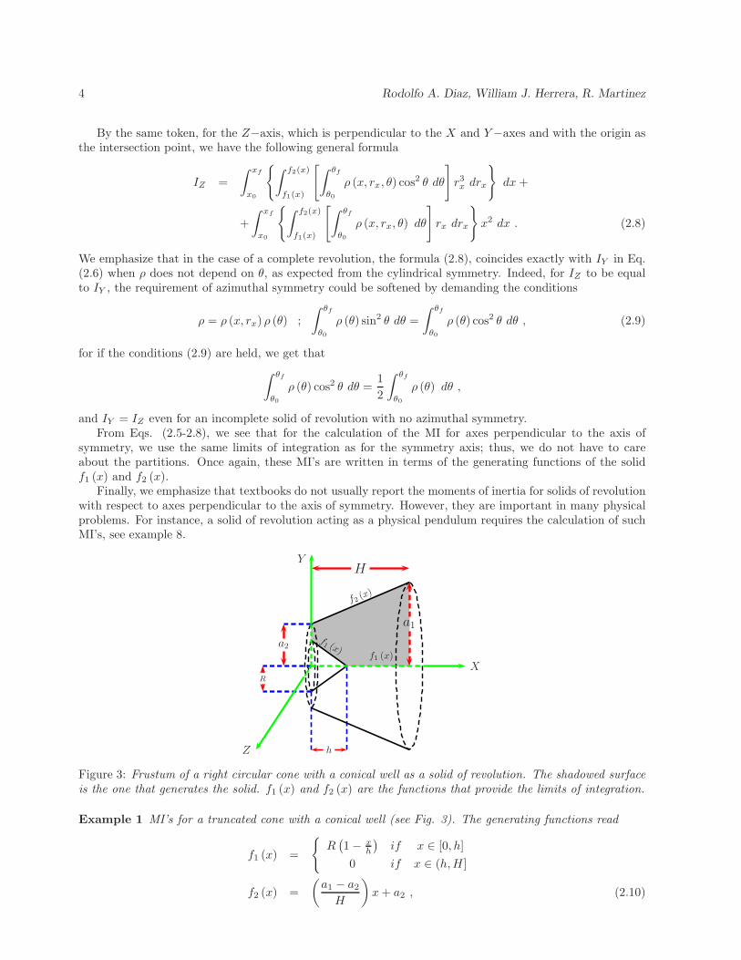
Figure 3: Frustum of a right circular cone with a conical well as a solid of revolution. The shadowed surfaceis the one that generates the solid. f1 (x) and f2 (x) are the functions that provide the limits of integration.

Example 1 MI’s for a truncated cone with a conical well (see Fig. 3). The generating functions read

f1 (x) =

{

R(

1− xh

)

if x ∈ [0, h]

0 if x ∈ (h,H ]

f2 (x) =

(

a1 − a2H

)

x+ a2 , (2.10)


where all the dimensions involved are displayed in Fig. 3. For uniform density, we can replace Eqs. (2.10)into Eqs. (2.4, 2.7) to get

IX =πρ

10

{

H(

a41 + a42 + a1a32 + a31a2 + a21a

22

)

−R4h}

IY = IZ =1

2IX +

πρH3

5

[

1

2a1a2 + a21 +

1

6a22 −

R2

6

(

h

H

)3]

.

It is more usual to give the radius of gyration (RG) instead of the MI. For this we calculate the mass of thesolid by using Eq. (A.1), finding

M =πρ

3

[

H(

a1a2 + a21 + a22)

−R2h]

. (2.11)

The radii of gyration become

K2X =

3{

H(

a41 + a42 + a1a32 + a31a2 + a21a

22

)

−R4h}

10 [H (a1a2 + a21 + a22)−R2h]

K2Y = K2

Z =K2

X

2+

3

5H3

[

12a1a2 + a21 +

16a

22 − R2

6

(

hH

)3]

[H (a1a2 + a21 + a22)−R2h]. (2.12)

By making R = 0 (and/or h = 0) we find the RG’s for the truncated cone. With R = 0 and a1 = 0, we getthe RG’s of a cone for which the axes Y and Z pass through its base. Making R = 0 and a2 = 0, we findthe RG’s of a cone but with the axes Y and Z passing through its vertex. Finally, by setting up R = 0, anda1 = a2; we obtain the RG’s for a cylinder. In many cases of interest, we need to calculate the MI’s for axesXCYCZC passing through the center of mass (CM), these MI’s can be calculated by finding the position ofthe CM with respect to the original coordinate axes, and using Steiner’s theorem (also known as “the parallelaxis theorem”). Applying Eqs. (A.2-A.4) the position of the CM for the truncated cone with a conical wellis given by (xCM , 0, 0) with

xCM =

[(

2a1a2 + 3a21 + a22)

H2 −R2h2]

4 [H (a1a2 + a21 + a22)−R2h]. (2.13)

Gathering Eqs. (2.12, 2.13) we find

K2XC

= K2X ; K2

YC= K2

Y − x2CM ; K2

ZC= K2

Z − x2CM .

2.3 Another alternative of calculation and a proof of consistency

In addition to the the parallel and the perpendicular axis theorems, there is another useful theorem aboutMI’s that is not usually included in common texts, namely [7]

IX + IY + IZ = 2∑

i

miR2i , (2.14)

where X,Y, Z are three mutually perpendicular intersecting axes, mi is the mass of the i−th particle and Ri

is its distance from the intersection. We shall see that our general formulae for MI’s of solids of revolution,fulfill the theorem. From Eqs. (2.2, 2.5, 2.8) we have

IX + IY + IZ = 2

∫ xf

x0

∫ f2(x)

f1(x)

∫ θf

θ0

(

x2 + r2x)

ρ (x, rx, θ) rx (dθ) (drx) (dx) . (2.15)

Moreover, if we take into account that the distance from the intersecting point (the origin of coordinates) tothe element of volume is R2 = x2 + r2x, and using Eq. (2.1) we conclude that

IX + IY + IZ = 2

∫

V

R2 dm , (2.16)


which is the continuous version of the theorem established in Eq. (2.14). As well as providing a proof ofconsistency, this theorem could reduce the task to estimate the MI’s, especially when a certain sphericalsymmetry is involved.

Further, it is interesting to see that the MI’s IX , IY , IZ , in Eqs. (2.2, 2.5, 2.8) fulfill the triangularinequalities

IX ≤ IY + IZ ,

and same for any cyclic change of the labels. The triangular inequalities follow directly from the definition ofMI, and are valid for any arbitrary object. Though the demostration of these inequalities is straightforward,they are not usually considered in the literature. In the case of thin plates, one of them becomes an equality.

Example 2 The following example shows the usefulness of the theorem of Eqs. (2.14, 2.16) in practicalcalculations. Let us consider the MI of a sphere centered at the origin, whose density is factorizable inspherical coordinates such that ρ = ρ(R). Where R is the distance from the origin of coordinates to thepoint. The symmetry of ρ leads to IX = IY = IZ and the theorem in Eq. (2.16) gives

3IX = 8π

∫ R0

0

ρ (R) R4 dR , (2.17)

the mass of the sphere is

M = 4π

∫ b

0

ρ(R)R2 dR , (2.18)

from which the moment of inertia can be written as

IX =2

3M

∫ b

0ρ(R)R4 dR

∫ b

0 ρ(R)R2 dR. (2.19)

We can calculate for instance, the classical MI of an electron in a hydrogen-like atom, with respect to an axis

that passes through its CM. For example, for the state (1, 0, 0) we have that ρ(R) = 2 (Z/a0)3/2

e−ZR/a0 ,where Z is the atomic number and a0 the Bohr’s radius. The MI becomes

IX =8me

Z2a20 .

3 MI’s of solids of revolution generated around the Y-axis

y

Z X

f x2( )

f x1( )

x0

xf

Y

yr df

ry drydy

df

x

ry

Figure 4: Solid of revolution generated around the Y−axis. The unit of integration is a piece of hoop withcross sectional area (dy) (dry) and length ry dφ.

By using a couple of generating functions f1 (x) and f2 (x) like in the previous section, we are able togenerate another solid of revolution by rotating such functions around the Y−axis instead of the X−axis


as Fig. 4 displays. In this case however, we should assume that x0 ≥ 0; such that all points in thegenerating surface have always non-negative x coordinates. Instead, we might allow the functions f1 (x),f2 (x) to be negative though still demanding that f1 (x) ≤ f2 (x) in the whole interval of x. In this case, itis more convenient to use another cylindrical system in which we define the coordinates (ry, y, φ), where ryis the distance from the Y−axis to the point, and the angle φ has been defined such that φ = 0 when thevector radius is parallel to the Z−axis (positive), increasing when going from Z (positive) to X (positive).One important comment is in order, since the surface that generates the solid lies on the XY−plane, the xcoordinate of any point of this surface (which is always non-negative according to our assumptions) coincideswith the coordinate ry, therefore we shall write f1 (ry) and f2 (ry) instead of f1 (x) , f2 (x) for the functionsthat bound the generating surface.

The procedure to evaluate the MI in the general case is analogous to the techniques used in section 2,the results are

IX =

∫ xf

x0

{

∫ f2(ry)

f1(ry)

[

∫ φf

φ0

ρ (ry, y, φ) cos2 φ dφ

]

dy

}

r3y dry +

+

∫ xf

x0

{

∫ f2(ry)

f1(ry)

[

∫ φf

φ0

ρ (ry , y, φ) dφ

]

y2 dy

}

ry dry , (3.1)

IY =

∫ xf

x0

{

∫ f2(ry)

f1(ry)

[

∫ φf

φ0

ρ (ry , y, φ) dφ

]

dy

}

r3y dry , (3.2)

IZ =

∫ xf

x0

{

∫ f2(ry)

f1(ry)

[

∫ φf

φ0

ρ (ry, y, φ) sin2 φdφ

]

dy

}

r3y dry +

+

∫ xf

x0

{

∫ f2(ry)

f1(ry)

[

∫ φf

φ0

ρ (ry , y, φ) dφ

]

y2 dy

}

ry dry . (3.3)

As before, these expressions become simpler in the case of a complete revolution with azimuthal symmetry,

IY = 2π

∫ xf

x0

[

∫ f2(ry)

f1(ry)

ρ (ry, y) dy

]

r3y dry , (3.4)

IX =1

2IY + 2π

∫ xf

x0

[

∫ f2(ry)

f1(ry)

ρ (ry , y) y2 dy

]

ry dry , (3.5)

and in this case IX = IZ , as expected from symmetry arguments. Further, assuming ρ = ρ (ry) theexpressions simplifies to

IY = 2π

∫ xf

x0

r3y ρ (ry) [f2 (ry)− f1 (ry)] dry , (3.6)

IX = IZ =1

2IY +

2π

3

∫ xf

x0

ρ (ry)[

f2 (ry)3 − f1 (ry)

3]

ry dry . (3.7)

We can verify again that the property IX = IZ ≥ IY /2 appears in the case of azimuthal symmetry, Eq.(3.5). This property is also satisfied in the case of incomplete solids of revolution, if conditions analogous toEq. (2.9) for the φ angle are fulfilled. Moreover, the theorem given by Eqs. (2.14, 2.16) is also held by theseformulae, giving an alternative way for the calculation. Finally, the triangular inequalities also hold.

These formulae are especially useful in the case in which the generating functions f1 (x), f2 (x) do notadmit inverses, since in such case we cannot find the corresponding inverse functions g1 (x), g2 (x) to generatethe same figure by rotating around the X−axis. This is the case in the following example


Y

X(R, 0)

Figure 5: Solid of revolution created by rotating the generating functions f1 (x) = 0, and f2 (x) = h +A sin

(

nπxR

)

around the Y−axis. The x variable lies in the interval [0, R]. From the picture it is clear thatone of the generators do not admit an inverse.

Example 3 Calculate the MI’s of a homogeneous solid formed by rotating the functions

f1 (x) = 0 ; f2 (x) = h+A sin(nπx

R

)

, (3.8)

around the Y −axis (see Fig. 5), where the functions are defined in the interval x ∈ [0, R], and n are positiveintegers. We demand h ≥ |A|, if n > 1; besides, if n = 1 and |A| > h we demand A > 0. These requirementsassure that f2 (x) ≥ f1 (x) for all x ∈ [0, R]. The mass of the solid, obtained from (A.8) reads

M =πR2ρ

nπ

[

nπh+ 2A (−1)n+1]

and replacing the generating functions into the Eqs. (3.6, 3.7) we get

K2Y =

R2

2

(

nπh+ 4A(6n−2π−2 − 1)(−1)n

nπh+ 2A(−1)n+1

)

K2X = K2

Z =K2

Y

2+

1

18

3nπh[2h2 + 3A2] + 4A(−1)n+1[9h2 + 2A2]

[nπh+ 2A(−1)n+1].

the position of the CM (obtained from Eqs. A.5-A.7), and the RG’s for axes that pass through the CM read

rCM = (0, yCM , 0) ; yCM =2nπh2 + nπA2 + 8Ah (−1)n+1

4[

nπh+ 2A (−1)n+1

]

K2XC

= K2X − y2CM ; K2

YC= K2

Y ; K2ZC

= K2Z − y2CM

Observe that f2 (x) does not have inverse. Hence, we cannot generate the same figure by constructing anequivalent function to be rotated around the X−axis∗.

Finally, it worths pointing out that by considering homogeneous solids of revolution, we obtain the sameexpressions derived with a different approach in Ref. [8].

4 Moments of inertia based on the contour plots of some figures

Suppose that we know the contour plots of certain solid in the XY plane, i.e. the surfaces shaped by theintersection between planes parallel to the XY plane and the solid (see Fig. 6). Assume that for a certainvalue of the z coordinate, the surface defined by the contour is bounded by the functions f1 (x, z) and f2 (x, z)in the y coordinate, and by x0 (z), xf (z) in the x coordinate, as shown in the frame on the upper rightcorner of Fig. 6. Let us form a thin plate of thick dz with the surface described above. In turn we can dividesuch thin plate into small rectangular boxes with surface dx dy and depth dz as shown in Fig. 6, it is wellknown from the literature [1] that the MI with respect to the X−axis in cartesian coordinates reads

IX =

∫

V

(

y2 + z2)

dm

∗Indeed, we can find the MI of this solid by rotating around the X−axis. We achieve it by splitting up the figure in severalpieces in the y coordinate, such that each interval in y defines a function. However, it implies to introduce more than twogenerating functions and the number of such generators increases with n, making the calculation more complex.


x z0 ( ) x zf ( )

Y

f x z1( , )

f x z2( , )

X

Y

dx

dydzy

x

X

dz

Z

Figure 6: Contour plots of a solid utilized to calculate its moments of inertia.

now, since our infinitesimal elements of volume are rectangular boxes with volume dV = dx dy dz, thecontribution of each rectangular box to the MI around the X−axis is given by

dIX =(

y2 + z2)

dm =(

y2 + z2)

ρ (x, y, z) dx dy dz ,

integrating over all variables, we obtain

IX =

∫ zf

z0

{

∫ xf (z)

x0(z)

[

∫ f2(x,z)

f1(x,z)

y2ρ dy

]

dx

}

dz +

∫ zf

z0

{

∫ xf (z)

x0(z)

[

∫ f2(x,z)

f1(x,z)

ρ dy

]

dx

}

z2 dz . (4.1)

The procedure for IY and IZ is analogous, the results are.

IY =

∫ zf

z0

{

∫ xf (z)

x0(z)

[

∫ f2(x,z)

f1(x,z)

ρ dy

]

x2 dx

}

dz +

∫ zf

z0

{

∫ xf (z)

x0(z)

[

∫ f2(x,z)

f1(x,z)

ρ dy

]

dx

}

z2 dz , (4.2)

IZ =

∫ zf

z0

{

∫ xf (z)

x0(z)

[

∫ f2(x,z)

f1(x,z)

y2ρ dy

]

dx

}

dz +

∫ zf

z0

{

∫ xf (z)

x0(z)

[

∫ f2(x,z)

f1(x,z)

ρ dy

]

x2 dx

}

dz . (4.3)

Once again, we can check that results (4.1, 4.2, 4.3) satisfy Eq. (2.16). This equation gives us anotherway to calculate the three MI’s. Finally, the formulae fulfill the triangular inequalities.

An interesting case arises when we consider the MI’s of thin plates. Suppose a thin plate lying on the XYplane. σ (x, y) denotes its surface density. This solid is generated by contour plots with volumetric density

ρ (x, y, z) = σ (x, y) δ (z) , (4.4)

where δ (z) denotes Dirac’s delta function. Replacing Eq. (4.4) into the general formula (4.1) we get

IX =

∫ zf

z0

H1 (z) δ (z) dz +

∫ zf

z0

H2 (z) δ (z) z2 dz ,

H1 (z) ≡∫ xf (z)

x0(z)

[

∫ f2(x,z)

f1(x,z)

y2σ (x, y) dy

]

dx ; H2 (z) ≡∫ xf (z)

x0(z)

[

∫ f2(x,z)

f1(x,z)

σ (x, y) dy

]

dx ,

and using the properties of δ (z) we get

IX = H1 (0) =

∫ xf (0)

x0(0)

[

∫ f2(x,0)

f1(x,0)

y2σ (x, y) dy

]

dx ,


the z coordinate is evaluated at zero all the time, hence there is only one contour, we write it simply as

IX =

∫ xf

x0

[

∫ f2(x)

f1(x)

y2σ (x, y) dy

]

dx . (4.5)

Similarly IY , IZ can be evaluated replacing (4.4) into (4.2) and (4.3)

IY =

∫ xf

x0

[

∫ f2(x)

f1(x)

σ (x, y) dy

]

x2 dx ; IZ = IX + IY . (4.6)

Hence, Eqs. (4.5, 4.6) give us the MI’s for a thin plate delimited by f1 (x) and f2 (x) and by x0, xf ; withsurface density σ (x, y). It worths noting that the second of Eqs. (4.6) arises from the application of (4.4)into (4.3) without assuming the perpendicular axes theorem; showing the consistency of our results†.

The formulae shown in this section are written in terms of generating functions as in the previoussections. However, these generators are functions of several variables. In developing these formulae we havenot used any particular symmetry; nevertheless, explicit use of some symmetries could simplify many specificcalculations as shown in the following examples.

a(z)

b(z)

X

Y

z z

a(z)

a1

a2

H

Z

Y

X

Figure 7: Frustum of a right elliptical cone. The shadowed surfaces show a contour for a certain value ofthe z coordinate, as well as its projection onto the XY−plane.

Example 4 Let us assume a truncated right elliptical cone as shown in Fig. 7. Such figure is characterizedby the semi-major and semi-minor axes in the base (denoted by a1,b1 respectively), its height H, and itssemi-major and semi-minor axes in the top (denoted by a2, b2 respectively). Suppose that the truncated coneis located such that the major base lies on the XY plane and the center of such major base is on the originof coordinates, as shown in Fig. 7. Now, since we are assuming that the figure is not oblique, then all thecontours (see right top on Fig. 7) are concentric ellipses centered at the origin, with the same eccentricity.Therefore, it is more convenient to describe such ellipses in terms of their eccentricity ε and the semi-majoraxis a (z). The contours are then delimited by

f1 (x, z) = −√

[

a (z)2 − x2]

(1− ε2) ; f2 (x, z) =

√

[

a (z)2 − x2]

(1− ε2) ,

x0 (z) = −a (z) ; xf (z) = a (z) ; ε ≡

√

1−(

b (z)

a (z)

)2

, (4.7)

where f1,2 (x, z) are the functions that generate the complete ellipse of semi-major axis a (z) and eccentricityε (independent of z). By simple geometric arguments, we could see that the semi-major axis of one contourof the truncated cone at certain height z is given by‡

a (z) = a1 +

(

a2 − a1H

)

z , (4.8)

†For students not accustomed to the Dirac’s delta function and its properties, we basically pass from the volume differentialρ dV to the surface differential σ dA.

‡The semi-minor axes follow a similar equation replacing a1,2 → b1,2. From such equations we can check that the quotientb(z)a(z)

is constant if we impose b1a1

= b2a2

. So the latter condition guarantees that the eccentricity remains constant.


Assuming that the density is constant Eq. (4.3) becomes

IZ =2ρ

3

(

√

1− ε2)3

∫ H

0

{

∫ a(z)

−a(z)

[

(

√

a (z)2 − x2

)3]

dx

}

dz

+2ρ√

1− ε2∫ H

0

{

∫ a(z)

−a(z)

[

√

a (z)2 − x2

]

x2 dx

}

dz ,

where we have already made the integration in y. Integration in x yields

IZ =πρ

4

(

2− ε2)

√

1− ε2

[

∫ H

0

a (z)4dz

]

, (4.9)

and taking into account the Eq. (4.8) we find

IZ =πρH

20

(

2− ε2)

√

1− ε2[

a41 + a42 + a1a32 + a31a2 + a21a

22

]

. (4.10)

Now, the mass of the figure is obtained from Eq. (A.12) and reads

M =πρH

3

√

1− ε2(

a21 + a22 + a1a2)

, (4.11)

therefore, the radius of gyration K2Z could be written as

K2Z =

3

20

(

2− ε2)

[

a41 + a42 + a1a32 + a31a2 + a21a

22

a1a2 + a21 + a22

]

.

Further, K2X and K2

Y can be derived from Eqs. (4.1, 4.2, 4.11) obtaining

K2X =

3

20

[(

1− ε2) (

a41 + a42 + a1a32 + a31a2 + a21a

22

)

+ 4H2(

a22 +16a

21 +

12a1a2

)]

(a21 + a22 + a1a2)

K2Y =

3

20

[(

a41 + a42 + a1a32 + a31a2 + a21a

22

)

+ 4H2(

a22 +16a

21 +

12a1a2

)]

(a21 + a22 + a1a2).

when ε = 0 we get the radii of gyration of a truncated cone with circular cross section. In addition, whenε = 0 and a2 = 0, the RG’s reduce to the expressions for a cone with the axes X and Y passing through itsbase. Setting ε = 0, a1 = 0, we also get the RG’s of a cone but with the X,Y axes passing through its vertex.Using ε = 0, a1 = a2 we obtain the RG’s of a cylinder. Finally, with a2 = 0 we get a cone with ellipticalcross section, and when a1 = a2 we obtain a cylinder with elliptical cross section. Now, if we are interestedin the MI for coordinates (XC , YC , ZC) passing through the CM, we should calculate the position of the CMfrom Eqs. (A.9-A.11) and use Steiner’s theorem obtaining

rCM = (0, 0, zCM) ; zCM =

(

2a1a2 + a21 + 3a22)

H

4 (a1a2 + a21 + a22), (4.12)

K2XC

= K2X − z2CM ; K2

YC= K2

Y − z2CM ; K2ZC

= K2Z . (4.13)

Example 5 Frustum of a right rectangular pyramid: The contour plots are rectangles. Since the figure isnot oblique, the ratios between the sides of the rectangle are constant. We define a1, b1 the length and widthof the major base; a2, b2 the dimensions of the minor base, and H the height of the solid, from which wehave

c ≡ b1a1

=b2a2

=b (z)

a (z)for all z ∈ [0, H ] ,


where it was assumed that the major base of the figure lies on the XY plane centered in the origin with thelengths a1 parallel to the X−axis and the widths b1 parallel to the Y−axis. The contours are delimited by

f1 (x, z) = − c

2a (z) ; f2 (x, z) =

c

2a (z) ,

x0 (z) = −a (z)

2; xf (z) =

a (z)

2.

The functional dependence on z is equal to the one in example 4, so a (z) is also given by Eq. (4.8). Theintegration of Eq. (4.3) gives

IZ =cρ

12

(

1 + c2)

∫ H

0

a (z)4dz ,

which is very similar to IZ in Eq. (4.9) for the truncated cone with elliptical cross section, and since a (z)in this example is also given by Eq. (4.8), the result of IZ for the truncated pyramid is straightforward byanalogy with Eq. (4.10)

IZ =cρH

60

(

1 + c2) (

a41 + a42 + a1a32 + a31a2 + a21a

22

)

,

the mass is obtained from Eq. (A.12) or by analogy with Eq. (4.11)

M =cρH

3

[

a21 + a22 + a1a2]

,

and the radius of gyration becomes

K2Z =

[

1 +(

b1a1

)2]

20

(

a41 + a42 + a1a32 + a31a2 + a21a

22

a21 + a22 + a1a2

)

.

When a2 = 0 we get the RG of a pyramid, if a1 = a2 we obtain the RG of the rectangular box. The RG’sK2

X , K2Y are given by

K2X =

3

5

112

(

b1a1

)2(

a41 + a42 + a1a32 + a31a2 + a21a

22

)

+H2(

12a1a2 +

16a

21 + a22

)

[a21 + a22 + a1a2],

K2Y =

3

5

112

(

a41 + a42 + a1a32 + a31a2 + a21a

22

)

+H2(

12a1a2 +

16a

21 + a22

)

[a21 + a22 + a1a2].

Finally, the expression for the position of the CM coincides with the results in example 4, Eq. (4.12) withthe corresponding meaning of a1, a2 in each case. The similarity of all these results with the ones in example4, comes from the equality in the modulation function of the contours a (z). More about it later.

Example 6 The general ellipsoid, centered at the origin of coordinates is described by

x2

a2+

y2

b2+

z2

c2= 1 , (4.14)

we shall assume that a ≥ b ≥ c. A more suitable way to write Eq. (4.14) is the following

y2 =(

a (z)2 − x2)

(

1− ε2)

,

a (z) ≡ a

√

1− z2

c2; b (z) ≡ b

√

1− z2

c2,

ε ≡

√

1−(

b (z)

a (z)

)2

=

√

1−(

b

a

)2

. (4.15)


For fixed values of z, we get ellipses whose projections onto the XY−plane are centered at the origin withsemi-major axis a (z) and semi-minor axis b (z). The Eqs. (4.15) show that such ellipses have constanteccentricity, and so we arrive to the delimited functions of Eqs. (4.7) with a (z) and b (z) given by Eqs.(4.15). Therefore, the first two integrations are performed in the same way as in the truncated elliptical coneexplained in example 4. Then we can use the result in Eq. (4.9) (except for the limits of integration in Z),the last integral is carried out by using Eqs. (4.15).

IZ =πρ

4

(

2− ε2)

√

1− ε2[∫ c

−c

a (z)4 dz

]

=4

15πa4cρ

(

2− ε2)

√

1− ε2 .

The mass of the ellipsoid is given by M = (4/3)πρabc = (4/3)πρa2c√1− ε2, so that

K2Z =

a2(

2− ε2)

5=

(

a2 + b2)

5,

it could be seen that the RG is independent of c, this dependence has been absorbed into the mass. Similarly,we can get the RG’s K2

X and K2Y applying Eqs. (4.1, 4.2), the results are

K2X =

1

5

(

b2 + c2)

; K2Y =

1

5

(

a2 + c2)

.

in this case all axes pass through the center of mass of the object.

Observe that the MI’s for the general ellipsoid (example 6) were easily calculated by resorting to theresults obtained for the truncated cone with elliptical cross section (example 4); it was because both figureshave the same type of contours (ellipses) though in each case such contours are modulated (scaled with thez coordinate) in different ways. This symmetry between the profiles of both contours permitted to makethe first two integrals in the same way for both figures, shortening the calculation of the MI for the generalellipsoid considerably.

As for the truncated cone with elliptical cross section (example 4) and the truncated rectangular pyramid(example 5), they show the opposite case, i. e. they have different contours but the modulation is of thesame type, this symmetry also facilitates the calculation of the MI of the truncated pyramid. We emphasizethat this kind of symmetries in either the contours or modulations, can be exploited for a great variety offigures to simplify the calculation of their MI’s.

5 Applications utilizing the calculus of variations

X

Y

x0xf

f x( )

Figure 8: Optimization of the generating function to minimize the moment of inertia of a solid of revolution,the mass is the constraint and the solid lies in the interval [x0, xf ] of length L.

In all the equations shown in this paper, the MI’s can be seen as functionals of some generating functions.For simplicity, we take a homogeneous solid of complete revolution around the X−axis with f1 (x) = 0. TheMI’s are functionals of the remaining generating function, from Eqs. (2.4, 2.7) and relabeling f2 (x) ≡ f (x),we get

IX [f ] =πρ

2

∫ xf

x0

f(

x′)4

dx′ , (5.1)

IY [f ] =IX [f ]

2+ πρ

∫ xf

x0

x′2f(

x′)2

dx′ . (5.2)


Then, we can use the methods of the calculus of variations (CV) §, in order to optimize the MI. To figureout possible applications, imagine that we should build up a figure such that under certain restrictions (thatdepend on the details of the design) we require a minimum of energy to set the solid at certain angularvelocity starting from rest. Thus, the optimal design requires the moment of inertia around the axis ofrotation to be a minimum.

As an specific example, suppose that we have a certain amount of material and we wish to make up asolid of revolution of a fixed length with it, such that its MI around a certain axis becomes a minimum. Todo it, let us consider a fixed interval [x0, xf ] of length L, to generate a solid of revolution of mass M andconstant density ρ (see Fig. 8). Let us find the function f (x), such that IX or IY become a minimum. Sincethe mass is kept constant, we use it as the fundamental constraint

M = πρ

∫ xf

x0

f(

x′)2

dx′ = constant. (5.3)

In order to minimize IX we should minimize the functional

GX [f ] =

∫ xf

x0

g(

f, x′)

dx′ = IX [f ]− λπρ

∫ xf

x0

f(

x′)2

dx′ (5.4)

where λ is the Lagrange’s multiplicator associated with the constraint (5.3). In order to minimize GX [f ],we should use the Euler-Lagrange equation [9]

δGX [f ]

δf(x)=

∂g(f, x)

∂f− ∂

∂x

∂g(f, x)

∂(df/dx)= 0 (5.5)

obtainingδGX [f ]

δf(x)= 2πρf (x)3 − 2πλρf (x) = 0 , (5.6)

whose non-trivial solution is given byf (x) =

√λ ≡ R . (5.7)

Analizing the second variational derivative we realize that this condition corresponds to a minimum.Hence, IX becomes minimum under the assumptions above for a cylinder of radius

√λ, such radius can be

obtained from the condition (5.3), yielding R2 = M/πρL and IX becomes

IX,cylinder =1

2

M2

πρL. (5.8)

Now, we look for a function that minimizes the MI of the solid of revolution around an axis perpendicularto the axis of symmetry. From Eqs. (5.2, 5.3), we see that the functional to minimize is

GY [f ] =IX [f ]

2+ πρ

∫ xf

x0

x′2f(

x′)2

dx′ − λπρ

∫ xf

x0

f(

x′)2

dx′ , (5.9)

making the variation of GY [f ] with respect to f (x) we get

f (x)2 = 2(

λ− x2)

≡ R2 − 2x2 , (5.10)

where we have written 2λ = R2. By taking x0 = −L/2, xf = L/2, the function obtained is an ellipse

centered at the origin with semimajor axis R along the Y−axis, semiminor axis R/√2 along the X−axis,

and with eccentricity ε = 1/√2. When it is revolved we get an ellipsoid of revolution (spheroid); such

spheroid is the solid of revolution that minimizes the MI with respect to an axis perpendicular to the axisof revolution. From the condition (5.3) we find

R2 =M

πρL+

L2

6. (5.11)

§The reader not familiarized with the methods of the CV, could skip this section without sacrifying the under-standing of the rest of the content. Interested readers can look up in the extensive bibliography concerning this topic,e.g. Ref. [9].


X-L/2 L/2

YR

L/2

Y

X

b)a)

R/ 2- R/ 2

Figure 9: (a) Elliptical function that generates the solids of revolution that minimize IY . The shaded regionis the one that generates the solid. (b) Truncated spheroid obtained when the shaded region is revolved.

In the most general case, the spheroid generated this way is truncated, as it is shown in Fig. 9, and thecondition R ≥ L/

√2 should be fulfilled for f (x) to be real. The spheroid is complete when R = L/

√2, and

the mass obtained in this case is the minimum one for the spheroid to fill up the interval [−L/2, L/2], thisminimum mass is given by

Mmin =πρL3

3, (5.12)

from (5.2), (5.10), (5.11) and (5.12) we find

IY,spheroid =MminL

2[

5µ+ 5µ2 − 1]

60; µ ≡ M

Mmin. (5.13)

Assuming that the densities and masses of the spheroid and the cylinder coincide, we estimate the quotients

IY,cylinder

IY,spheroid

=

(

5µ+ 5µ2 − 1)

5µ (µ+ 1)< 1,

IX,cylinder

IX,spheroid

=

(

1 +1

5µ−2

)−1

< 1 . (5.14)

Eqs. (5.14) show that IY,sph < IY,cyl while IX,cyl < IX,sph. In both cases if M >> Mmin the MI’s of thespheroid and the cylinder coincide, it is because the truncated spheroid approaches the form of a cylinderwhen the amount of mass to be distributed in the interval of length L is increased.

On the other hand, in many applications what really matters are the MI’s around axes passing throughthe CM. In the case of homogeneous solids of revolution the axis that generates the solid passes throughthe CM, but this is not necessarily the case for an axis perpendicular to the former. If we are interested inminimizing IYC

, i.e. the MI with respect to an axis parallel to Y and passing through the CM, we shouldwrite the expression for IYC

by using the parallel axis theorem and by combining Eqs. (5.2, 5.3, A.2)

IYC[f ] =

IX [f ]

2+ πρ

∫ xf

x0

x′2f(

x′)2

dx′

− πρ∫ xf

x0f (x′)2 dx′

[∫ xf

x0

x′f(x′)2 dx′

]2

, (5.15)

thus, the functional to be minimized is

GYC[f ] = IYC

[f ]− λπρ

∫ xf

x0

f(

x′)2

dx′ , (5.16)

after some algebra, we arrive to the following minimizing function

f (x)2 = R2 − 2 (x− xCM )2 , (5.17)

where we have written 2λ = R2. It corresponds to a spheroid (truncated, in general) centered at the point(xCM , 0, 0) as expected, showing the consistency of the method.

Finally, it worths remarking that the techniques of the CV shown here can be extrapolated to morecomplex situations, as long as we are able to see the MI’s as functionals of certain generating functions. Thesituations shown here are simple for pedagogical reasons, but they open a window for other applications withother constraints¶, for which the minimization cannot be done by intuition. For instance, if our constraintconsists of keeping the surface constant, the solutions are not easy to guess, and should be developed byvariational methods.

¶Another possible strategy consists of parameterizing the function f (x), and find the optimal values for theparameters.


6 Analysis and conclusions

Most textbooks report MI’s for only a few number of simple figures. By contrast, the examples illustratedin this work have been chosen to be more general, and can also cover many particular cases. On the otherhand, in the specific case of solids of revolution, only the MI with respect to the symmetry axis is usuallyreported. Perhaps the most advantageous feature of the methods developed in this paper is that the threemoments of inertia IX , IY , IZ can be calculated by applying the same limits of integration, and we do nothave to worry about the partitions. It is because all three moments of inertia are written in terms of thegenerating functions of the solid. For instance, any solid of revolution acting as a physical pendulum providesan example in which the MI with respect to an axis perpendicular to the axis of symmetry is necessary, anspecific case is example 8 for the Gaussian bell (see appendix B.1). Moreover, we examine the conditions forthe perpendicular MI’s to be degenerate, we find that this degeneracy occurs even for inhomogeneous solidsas long as the density has an azimuthal symmetry. Remarkably, even for incomplete solids of revolution withthe azimuthal symmetry broken, such degeneracy may occur under certain conditions.

Finally, we point out that for solids of revolution in which densities depend only on the height of thesolid, the expressions for the MI become simple integrals, such fact makes the integration process mucheasier. Simple integrals are advantageous even in the case in which we cannot evaluate them analytically.Numerical methods to evaluate MI’s utilize typically the geometrical shape of the body; instead, numericalmethods for simple integrals are usually easier to manage.

As for the technique of contour plots, we can realize that many different figures could have the same typeof contours though a different modulation of them, one specific example is the case of a cone with ellipticalcross section and a general ellipsoid, in both solids the contours are ellipses but they are modulated (scaledwith the z coordinate) in different ways. On the other hand, in some cases the contours are different butthe modulation is of the same type, for example a cone and a pyramid has the same type of modulation(scaling) but their contours are totally different. In both situations we can save a lot of effort by makingprofit from the similarities. The reader can check the examples 4, 5 and 6, in order to figure out the way inwhich we can exploit these symmetries in practical calculations.

Furthermore, textbooks always consider homogeneous figures to estimate the MI, assumption that is notalways realistic. As for our formulae, though they simplify considerably when we consider homogeneousbodies, the methods are tractable in many cases when inhomogeneous objects are considered, allowing morerealistic results.

Another interesting remark is that these methods can be used to calculate products of inertia in the casein which the complete tensor of inertia is necessary. Moreover, expressions for the CM proceed by similararguments, and the appendix A, shows some formulae for the CM of solids of revolution and solids built upby contour plots. In such expressions we realize that the same limits of integration defined for the calculationof the MI’s are used to calculate the CM.

Finally, since all our formulae for MI’s depend on certain generating functions, we can see the MI ofa wide variety of figures as a functional, making the MI’s suitable to utilize methods of the calculus ofvariations. In particular, minimization of the MI under certain restrictions is possible utilizing variationalmethods, it could be very useful in applied physics and engineering.

The authors acknowledge to Dr. Hector Munera for revising the manuscript.

A Calculation of centers of mass

A.1 CM of solids of revolution generated around the X − axis

Taking into account the definition of the center of mass for continuous systems

~rCM =

∫

~r dm∫

dm,

we can get general formulae to calculate the CM of a solid by using a similar procedure to the one followedto get MI’s. First of all we calculate the total mass based on the density and the geometrical shape of the


body. In the case of solids of revolution around the X−axis, the total mass of the solid is given by

M =

∫

dm =

∫ xf

x0

{

∫ f2(x)

f1(x)

[

∫ θf

θ0

ρ (x, rx, θ) dθ

]

rx drx

}

dx , (A.1)

and the CM coordinates read

XCM =1

M

∫ xf

x0

{

∫ f2(x)

f1(x)

[

∫ θf

θ0

ρ (x, rx, θ) dθ

]

rx drx

}

x dx , (A.2)

YCM =1

M

∫ xf

x0

{

∫ f2(x)

f1(x)

[

∫ θf

θ0

ρ (x, rx, θ) cos θ dθ

]

r2x drx

}

dx , (A.3)

ZCM =1

M

∫ xf

x0

{

∫ f2(x)

f1(x)

[

∫ θf

θ0

ρ (x, rx, θ) sin θ dθ

]

r2x drx

}

dx , (A.4)

the limits of integrations are the ones defined in Sec. 2.1. In the case of complete revolution with ρ = ρ (x, rx),we obtain YCM = ZCM = 0, as expected from the cylindrical symmetry.

A.2 CM of solids of revolution generated around the Y − axis

By using the coordinate system and the limits of integration defined in Sec. 3, we can evaluate the CM forsolids of revolution generated around the Y−axis obtaining

XCM =1

M

∫ xf

x0

{

∫ f2(ry)

f1(ry)

[

∫ φf

φ0

sin(φ)ρ (ry, y, φ) dφ

]

dy

}

r2y dry , (A.5)

YCM =1

M

∫ xf

x0

{

∫ f2(ry)

f1(ry)

[

∫ φf

φ0

ρ (ry, y, φ) dφ

]

y dy

}

ry dry , (A.6)

ZCM =1

M

∫ xf

x0

{

∫ f2(ry)

f1(ry)

[

∫ φf

φ0

ρ (ry, y, φ) cos(φ) dφ

]

dy

}

r2y dry , (A.7)

M =

∫ xf

x0

{

∫ f2(ry)

f1(ry)

[

∫ φf

φ0

ρ (ry , y, φ) dφ

]

dy

}

ry dry . (A.8)

In the case of a complete revolution with ρ = ρ (ry, y), we get XCM = ZCM = 0, due to the cylindricalsymmetry.

A.3 CM of solids formed by contour plots

In this case, we use the limits of integration defined in Sec. 4. The CM coordinates read

xCM =1

M

∫ zf

z0

{

∫ xf (z)

x0(z)

[

∫ f2(x,z)

f1(x,z)

ρ (x, y, z) dy

]

x dx

}

dz , (A.9)

yCM =1

M

∫ zf

z0

{

∫ xf (z)

x0(z)

[

∫ f2(x,z)

f1(x,z)

ρ (x, y, z) y dy

]

dx

}

dz , (A.10)

zCM =1

M

∫ zf

z0

{

∫ xf (z)

x0(z)

[

∫ f2(x,z)

f1(x,z)

ρ (x, y, z) dy

]

dx

}

z dz , (A.11)

M =

∫ zf

z0

{

∫ xf (z)

x0(z)

[

∫ f2(x,z)

f1(x,z)

ρ (x, y, z) dy

]

dx

}

dz . (A.12)


B Some additional examples for the calculation of moments of

inertia

In this appendix we carry out additional calculations of moments of inertia for some specific figures, byapplying the formulae written in sections 2, 3 and 4; in order to illustrate the power of the methods.

B.1 Examples of moments of inertia for solids of revolution

a-a

Y

h

b

X

Y

X

B

A

a) b)

Z

Figure 10: On left: cylindrical wedge generated around the Y−axis. On right: A bell modelated by two Gauss’distributions rotating around the Y−axis, the bell tolls around an axis perpendicular to the sheet that passesthrough the point B

Example 7 MI for a cylindrical wedge (see Fig. 10). Let us consider a cylinder of height h and radius b,whose density is given by

ρ(φ) =

{

ρ, α ≤ φ ≤ 2π − α

0, − α < φ < α

and that is generated around the Y−axis by means of the functions f1 (x) = 0 and f2 (x) = h. From Eq.(A.8) and Eqs.(3.1-3.3) we find

M = (π − α)ρhb2 ,

IX = M

[

b2

8

(

2− sin 2α

(π − α)

)

+h2

3

]

; IY =Mb2

2; IZ = M

[

b2

8

(

2 +sin 2α

(π − α)

)

+h2

3

]

.

In order to calculate the moments of inertia from axes passing through the center of mass we use Eqs.(A.5-A.7) to get

XCM = 0 ; YCM =h

2; ZCM = −2

3

b

(π − α)sinα.

Example 8 MI’s for a Gaussian Bell. Let us consider a homogeneous hollow bell, which can be reasonablydescribed by a couple of Gaussian distributions (see Fig. 10).

f1(x) = Ae−αx2

; f2(x) = Be−βx2

,

where α, β,A,B are positive numbers, A < B, and α > β. The MI’s are obtained from (3.6, 3.7)

IY = πρ

[

B

β2− A

α2

]

; IX = IZ =πρ

2

[

B

β2− A

α2

]

+πρ

9

[

B3

β− A3

α

]

Besides, the mass and the center of mass position read

M = πρ

[

B

β− A

α

]

; YCM =1

4

[

αB2 − βA2

αB − βA

]

; XCM = ZCM = 0 .


When the bell tolls, it rotates around an axis perpendicular to the axis of symmetry that passes the top of thebell. Thus, this is a real situation in which the perpendicular MI is required. On the other hand, owing tothe cylindrical symmetry, we can calculate this moment of inertia by taking any axis parallel to the X−axis.In our case the top of the bell corresponds to y = B, and using Steiner’s theorem it can be shown that

IX,B = IX +MB(B − 2YCM )

IX,B =πρ

18α2β2

[

α2B(9 + 11B2β) + β2A(9ABα− 2A2α− 18B2α− 9)]

.

B.2 Examples of MI’s by the method of contourplots

Example 9 A thin elliptical plate: for this bidimensional object, we can use Eqs. (4.5, 4.6), the delimitedfunction can be taken from (4.7) but with z = 0. The results are

IX = Mb2

4; IY = M

a2

4,

IZ = M

(

a2 + b2)

4; M = πσab .

once again, these axes passes through the center of mass of the figure.

h1

h2

a1

a2

a3

Y

X

Figure 11: Arbitrary quadrilateral, the dimensions are indicated in the drawing.

Example 10 An arbitrary quadrilateral, (see Fig. 11): This is a bidimensional figure, so we apply Eqs.(4.5, 4.6). The bounding functions are given by

f1 (x) = 0 ,

f2 (x) =

h1

a1x if 0 ≤ x ≤ a1

(h2−h1)a2

x+ h1(a1+a2)−h2a1

a2if a1 < x ≤ a1 + a2

−h2

a3x+ h2

a3(a1 + a2 + a3) if a1 + a2 < x ≤ a1 + a2 + a3

and the moments of inertia read

IX =σ

12

[

a2 (h1 + h2)(

h21 + h2

2

)

+ h31a1 + h3

2a3]

(B.1)

IY =σ

12

[

12a1a2a3h2 +(

4a1a22 + 3a31 + a32

)

h1 +(

4a2a23 + 3a32 + a33

)

h2

+6a21a2 (h1 + h2) + 4a1h2

(

2a22 + a23)

+ 6a3h2

(

a21 + a22)]

(B.2)

IZ = IX + IY (B.3)


the center of mass coordinates are given by

xCM =σ

6M[3a1a2 (h1 + h2) + 3a3h2 (a1 + a2)

+h1

(

2a21 + a22)

+ h2

(

2a22 + a23)]

(B.4)

yCM =σ

6M

[

a2h1h2 + (a1 + a2)h21 + (a2 + a3)h

22

]

(B.5)

withM =

σ

2[a1h1 + a2 (h1 + h2) + a3h2] (B.6)

The quantities IX , yCM , and M ; are invariant under traslations in x, for example IX might be calculatedas

IX =σ

3

∫ xf

x0

f2 (x)3 dx =

σ

3

∫ xf−∆x

x0−∆x

f2 (u+∆x)3 du

where we have performed a traslation ∆x to the left. It is equivalent to make the change of variablesu = x−∆x. This property can be used to evaluate the integrals easier. Specifically, the piece of Fig. 11 lyingin the interval a1 < x ≤ a1 + a2, can be traslated to the origin by using ∆x = a1; and the piece of this figurelying at a1 + a2 < x ≤ a1 + a2+ a3 can be also traslated to the origin with ∆x = a1+ a2. On the other hand,though the quantities IY and xCM are not invariant under such traslations, the same change of variablessimplifies their calculations. This strategy is very useful in solids or surfaces that can be decomposed bypieces (i.e. when at least one of the generator functions is defined by pieces). For example, the same changeof variables could be used if we are interested in the solid of revolution generated by the surface of Fig. 11.

Finally, from Eqs. (B.1-B.6) we can obtain many particular cases, some of them are

• h1 = h2 trapezoid.

• a1 = h1 = 0 arbitrary triangle.

• a2 = 0, a1 = a3 = h1√3= h2√

3≡ L

2 equilateral triangle of side length L.

• a1 = h1 = 0, a2 = a3 = h2√3≡ L

2 equilateral triangle of side length L.

• a1 = a3 = h1 = 0 triangle with a right angle.

• h2 = h1, a2 = 0 arbitrary triangle.

• a1 = a3 = 0, h2 = h1 rectangle.

C Table of moments of inertia

In table 1 on page 22, the moments of inertia for a variety of solids of revolution generated around theY−axis are displayed, such table includes the function generators and any other information necessary tocarry out the calculations by means of our methods. The surfaces that generates the solids are displayed inFig. 12. Observe that the first of these surfaces generates a torus with elliptical cross section and the secondone generates a truncated hollow cone.

Finally, there are some conditions for certain parameters of these figures. In Fig. (d), a > 0, and b > 2a;in Fig. (e) b > 0, and a > 0, in Fig. (f), n > 0; for Fig. (g), n > −2/3; in Figs. (c) and (h) a can also benegative.


x

y

0

R a- R+a

bR

-b

x

y

0 a b

h

cx

y

0R

A

0x

y

b ca

Aa2

A b-a( )2

x

y

0ba

Aa2

0x

y

0b0

x

y

0b

Abn

x

y

0b0

A

a) b) c) d)

e) f) g) h)

00

e-ax2A

eaxA

Figure 12: Surfaces that generates the solids whose moments of inertia appears on the table 1

References

[1] D. Kleppner and R. Kolenkow, An introduction to mechanics (McGRAW-HILL KOGAKUSHA LTD,1973); R. Resnick and D. Halliday, Physics (Wiley, New York, 1977), 3rd Ed.; M. Alonso and E.Finn, Fundamental University Physics, Vol I, Mechanics (Addison-Wesley Publishing Co., Massachus-sets, 1967).

[2] R. C. Hibbeler, Engineering Mechanics Statics, Seventh Ed. (Prentice-Hall Inc., New York,1995).

[3] Louis Leithold, The Calculus with Analytic Geometry (Harper & Row, Publishers, Inc. , New York,1972), Second Ed.; E. W. Swokowski, Calculus with Analytic Geometry (PWS-KENT Publishing Co.,Boston Massachusetts, 1988), Fourth Ed.; S. K. Stein, Calculus and Analytic Geometry (Mc-Graw HillBook Co. 1987), Fourth Ed.

[4] R. Szmytkowski, “Simple method of calculation of moments of inertia”, Am. J. Phys. 56, 754-756 (1988);R. Rabinoff “Moments of inertia by scaling arguments: How to avoid messy integrals” Am. J. Phys. 53,501-502 (1985).

[5] Carl M. Bender and Lawrence R. Mead, “D-dimensional moments of inertia” Am. J. Phys. 63, 1011-1014(1995); J. Casey and S. Krishnaswamy, “Problem: Which rigid bodies have constant inertia tensors?”Am. J. Phys. 63, 276-281 (1995); P. K. Aravind, “A comment on the moment of inertia of symmetricalsolids” Am. J. Phys. 60, 754-755 (1992); P. K. Aravind, “Gravitational collapse and moment of inertia ofregular polyhedral configurations” Am. J. Phys. 59, 647-652 (1991); J. Satterly, “Moments of Inertia ofSolid Rectangular Parallelopipeds, Cubes, and Twin Cubes, and Two Other Regular Polyhedra” Am. J.Phys. 25, 70-78 (1957) ; J. Satterly, “Moments of Inertia of Plane Triangles” Am. J. Phys. 26, 452-453(1958).

[6] W. N. Mei and Dan Wilkins, “Making a pitch for the center of mass and the moment of inertia” Am.J. Phys. 65, 903-907 (1997); Joseph C. Amato and Roger E. Williams and Hugh Helm, “A black boxmoment of inertia apparatus” Am. J. Phys. 63, 891-894 (1995).

[7] J. F. Streib, “A theorem on moments of inertia” Am. J. Phys. 57, 181 (1989).

[8] Rodolfo A. Diaz, William J. Herrera, R. Martinez, http://xxx.lanl.gov/list/physics/0507 Preprint num-ber: physics/0507172.

[9] G. Arfken. Mathematical methods for physicists, Second Ed. (Academic Press, International Edition,1970) Chap. 17.

http://xxx.lanl.gov/list/physics/0507

http://arxiv.org/abs/physics/0507172

22

Rodolfo

A.Diaz,

Willia

mJ.Herrera

,R.Martin

ez

Fig f1(x) f2(x) x0 xf M IY IX = IZ YCM

a −f2(x)b√

a2−(x−R)2

a R− a R+ a 2π2ρRba M(R2 + 34a

2) M8 (4R2 + 3a2 + 2b2) 0

b 0h, a < x < b

h c−xc−b , b ≤ x ≤ c

a c

πρh3 (b2 + bc

+c2 − 3a2)

πρh10 [b4 + b3c+ b2c2

+bc3 + c4 − 5a4]

Iy2 + πρh3×(3bc+6b2+c2−10a2)

30

h4

(3b2+2bc+c2−6a2)[b2+bc+c2−3a2]

c 0 Aeax 0 b

2πAρa2

(

eabab

−eab + 1)

2πAρa4 eab

(

a3b3 − 3a2b2

+6(

ab− 1 + e−ab))

12IY + 2π

27a2 ρA3×

(

e3ab (3ab− 1) + 1)

A8

(e2ab(2ab−1)+1)(eab(ab−1)+1)

d A(x− a)2 A(b− a)2 0 b πAρb3

6 (3b− 4a) M b2

5 (5b−6a3b−4a )

Iy2 + b3ρA3π

84 (21b5

−120ab4 + 280a2b3

−336a3b2 + 210a4b− 56a5)

A(10b3+45a2b−36ab2−20a3)5(3b−4a)

e 0 A(x− a)2 0 b

16πρAb

2(3b2

−8ab+ 6a2)

πρb4A30 (10b2

−24ab+ 15a2)

Iy2 + b2ρA3π

84

[

28a6 + 7b6−

48ab5 − 112a5b+ 140a2b4

−224a3b3 + 210a4b2]

A5 (15a

4 + 5b4 − 24ab3

−40a3b+ 45a2b2)×1

(3b2−8ab+6a2)

f Axn Abn 0 b πρAbn+2 nn+2 M b2

2n+2n+4

Iy2 +MA2b2n n+2

3n+2 A n+22n+2b

n

g 0 Axn 0 b 2πρA bn+2

n+2 Mb2 n+2n+4

Iy2 + 1

3Mn+23n+2A

2b2n A4

bn(n+2)n+1

h 0 Ae−ax2

0 b πρA1−e−b2a

a M 1−e−ab2 (1−ab2)

a(1−e−ab2 )

IY2 + MA2(1+e−ab2+e−2ab2 )

9A4

(1−e−2ab2 )

(1−e−ab2 )

Table

1:Moments

ofinertia

foravariety

ofsolid

sofrev

olutio

ngenera

tedaroundtheY−

axis,

thesurfa

cesthatgenera

testhesolid

sare

disp

layed

inFig.12

minimizemomentsofinertia arXiv:physics/0404005v2 … · 2018-08-27 · 2...

Documents

Transcript of minimizemomentsofinertia arXiv:physics/0404005v2 … · 2018-08-27 · 2...