Mincostflow Notes

Discrete OptimizationMA3233 Course Notes

William J. Martin IIIMathematical Sciences

Worcester Polytechnic Institute

November 30, 2012

c© 2010 William J. Martin IIIall rights reserved

Contents

Contents i

1 Basic Graph Theory 21.1 Start at the beginning . . . . . . . . . . . . . . . . . . . . . . . . . . 21.2 Coloring and Flows . . . . . . . . . . . . . . . . . . . . . . . . . . . . 71.3 Factors in graphs . . . . . . . . . . . . . . . . . . . . . . . . . . . . . 101.4 The Menagerie . . . . . . . . . . . . . . . . . . . . . . . . . . . . . . 12

2 Trees and the Greedy Algorithm 172.1 The greedy algorithm . . . . . . . . . . . . . . . . . . . . . . . . . . . 182.2 Prim’s Algorithm . . . . . . . . . . . . . . . . . . . . . . . . . . . . . 212.3 The Menagerie . . . . . . . . . . . . . . . . . . . . . . . . . . . . . . 22

3 Basic Search Trees 263.1 Generic Search . . . . . . . . . . . . . . . . . . . . . . . . . . . . . . 263.2 Breadth-first and depth-first search . . . . . . . . . . . . . . . . . . . 273.3 The Menagerie . . . . . . . . . . . . . . . . . . . . . . . . . . . . . . 31

4 Shortest Path Problems 334.1 The Landscape . . . . . . . . . . . . . . . . . . . . . . . . . . . . . . 334.2 Dijkstra’s algorithm . . . . . . . . . . . . . . . . . . . . . . . . . . . . 344.3 Proof of correctness . . . . . . . . . . . . . . . . . . . . . . . . . . . . 374.4 Other algorithms for shortest paths . . . . . . . . . . . . . . . . . . . 384.5 The Menagerie . . . . . . . . . . . . . . . . . . . . . . . . . . . . . . 40

5 Linear Programming 455.1 LP problems . . . . . . . . . . . . . . . . . . . . . . . . . . . . . . . . 455.2 Shortest path . . . . . . . . . . . . . . . . . . . . . . . . . . . . . . . 475.3 LP algorithms . . . . . . . . . . . . . . . . . . . . . . . . . . . . . . . 495.4 LP duality . . . . . . . . . . . . . . . . . . . . . . . . . . . . . . . . . 50

i

ii CONTENTS

5.5 The Menagerie . . . . . . . . . . . . . . . . . . . . . . . . . . . . . . 53

6 NP-coNP Predicates 556.1 Polynomial time . . . . . . . . . . . . . . . . . . . . . . . . . . . . . . 556.2 Non-deterministic polynomial time . . . . . . . . . . . . . . . . . . . 586.3 The big conjectures . . . . . . . . . . . . . . . . . . . . . . . . . . . . 596.4 Examples . . . . . . . . . . . . . . . . . . . . . . . . . . . . . . . . . 606.5 NP-Complete and NP-hard problems . . . . . . . . . . . . . . . . . . 636.6 Landau notation . . . . . . . . . . . . . . . . . . . . . . . . . . . . . 656.7 The Menagerie . . . . . . . . . . . . . . . . . . . . . . . . . . . . . . 67

7 Network Flows 697.1 Statement of the problem . . . . . . . . . . . . . . . . . . . . . . . . 697.2 The Ford-Fulkerson algorithm . . . . . . . . . . . . . . . . . . . . . . 707.3 The Max-Flow Min-Cut Theorem . . . . . . . . . . . . . . . . . . . . 737.4 The Menagerie . . . . . . . . . . . . . . . . . . . . . . . . . . . . . . 76

8 Dinic’s Algorithm for Network Flows 788.1 The Dinic algorithm for maximum flow . . . . . . . . . . . . . . . . . 788.2 An example . . . . . . . . . . . . . . . . . . . . . . . . . . . . . . . . 808.3 Analysis of the Dinic algorithm . . . . . . . . . . . . . . . . . . . . . 838.4 The Menagerie . . . . . . . . . . . . . . . . . . . . . . . . . . . . . . 84

9 The Minimum Cost Flow Problem 869.1 Finding minimum cost flows . . . . . . . . . . . . . . . . . . . . . . . 869.2 Linear programming and the Magic Number Theorem . . . . . . . . . 899.3 The Menagerie . . . . . . . . . . . . . . . . . . . . . . . . . . . . . . 90

Bibliography 91

Preface

These notes grew out of my teaching of the course MA3233, “Discrete Optimization”at Worcester Polytechnic Institute in Fall 2008 and Fall 2010. I am indebted tothe students for helpful comments and corrections on the material included here. Inparticular, the 2008 class produced scribe notes (mostly handwritten) on the lecturesin that first delivery of the course.

The notes here are influenced by several sources. In our course, we used the bookof Papadimitriou and Steiglitz as a guide; as a result, the notation used here mostlyfollows that book. But our audience is different: rather than graduate students, weare addressing these notes to second- and third-year undergraduates in mathematicsand related disciplines. And our focus here is only on discrete optimization; linearprogramming, non-linear optimization, and basic graph theory are taught in othercourses at WPI and so these subjects are brought into purview only on an as-neededbasis. Finally, an undergraduate course at WPI consists of 28 lectures packed intoseven weeks, with the net effect that homeworks and exams are less conceptual andmore skill-oriented than at comparable universities.

I have benefited over the years from several teachers. In particular, I routinelyconsult my personal course notes from C&O 650, taught by Jack Edmonds at theUniversity of Waterloo in the fall of 1987. I also recycle ideas picked up from BillPulleyblank’s offering of C&O 652 in Winter 1988, Rama Murty’s lectures on thematching lattice and discussions of computational complexity theory with variouscolleagues, including James Currie, Dan Dougherty, Stan Selkow, and Madhu Sudan.

The notes are typeset using the LaTeX memoir document class. I am gratefulto Bill Farr at Worcester Polytechnic Institute, not only for teaching me about thisclass, but also for teaching me about teaching, and for that extra inspiration thatgets a writing project moving.

1

One

Basic Graph Theory

Oct. 25, 2012

In this course, we consider optimization problems over discrete (usually finite)spaces. By “space” here, I informally mean a set with some specified structure onthe set such as an assortment of binary relations and functions on that set and thoserelations. A unifying concept for such objects is that of a graph. In this lecture, wedefine graphs, directed graphs, and some of the common substructures that we workwith in these graphs in our study of optimization.

1.1 Start at the beginning

An undirected graph is a very intuitive, simple mathematical structure. Since weshall be dealing with these quite a lot, let’s begin by defining them.

Definition 1.1.1. A graph is an ordered pair G = (V, E) where V is a finite set andE is a finite collection (perhaps with repetition) of unordered pairs from V . Themembers of V are called vertices (or nodes) and the members of E are called edges.

Technically, what we have defined here is a finite, undirected graph since we assumeV to be a finite set and the edges are unordered pairs of vertices. While we will havelittle use for infinite graphs in this course, we will study directed graphs, which will bedefined below. If the vertex set or edge set of a graph G have not been pre-specified,it will be convenient to use V (G) and E(G) to denote these sets, respectively.

In Figure 1.1, we consider three small examples of graphs.

The graph on the left in Figure 1.1 has vertex set V (G) = A, B, C,Dand edge set E(G) = e1 = [A, B], e2 = [A, B], e3 = [A, C], e4 = [A, D], e5 =

2

1.1. START AT THE BEGINNING 3

Figure 1.1: Three graphs.

[B, B], e6 = [C, D], e7 = [C, D]. The center graph, H, has vertex setV (H) = x1, x2, x3 and edge set E(H) = [x1, x2], [x2, x2]. GraphK, on the right, has vertex set V (K) = u, v, w, x, y and edge setE(K) = [u, w], [v, w], [w, x], [x, y].

As seen in these examples, a small graph is often best described by a drawing.Each vertex is represented by a dot or circle in the plane and each edge is representedby a continuous path joining the two vertices in it, i.e., the ends or endpoints of edgee = [u, v] are the vertices u and v. It is important to note that the drawing is intendedto convey no more information than the combinatorial structure of the graph itself:which vertices are the ends of each edge. The shape of the edge, or the fact thattwo edges may cross somewhere other than an endpoint, is irrelevant to the structurebeing defined or pictorially described. (Try drawing a graph with five vertices andten edges, one for each pair of distinct vertices. Can you do this without making twoedges cross in the middle?) In spite of this potential for confusion, we frequently usethese graph drawings to convey information about graphs and algorithms on them.

Let G = (V, E) be a graph. An edge of the form e = [u, u] is called a loop in Gand a “loopless” graph is a graph with no loops, of course. If e, f ∈ E have the sameexact ends — say e = [u, v] and f = [u, v], for example — then we say G has multipleedges. A simple graph is an undirected graph with no loops or multiple edges. Forexample, in Figure 1, Graph K is simple, but graphs G and H are not simple.

A more precise definition of a graph can be given which avoids the set-theoreticambiguity of multiple edges. Formally, a graph is a triple G = (V, E, I) where Vand E are sets and I ⊂ V × E is an incidence relation with the property that eache ∈ E appears either once or twice as the second coordinate of some ordered pair

4 CHAPTER 1. BASIC GRAPH THEORY

in I. (Edge e is “incident” with exactly one or exactly two elements of V .) In ourexploration, we will not need this level of formality.

A vertex v and an edge e in a graph G are said to be incident if v is an end ofedge e. Two vertices u and v are said to be adjacent if [u, v] is an edge. (Let uswrite u ∼ v to denote the adjacency relation.) The degree of a vertex in a graph Gis defined to be the number of edges incident to that vertex, with the rule that loopscount twice. The degree of vertex v in a graph G is denoted deg(v) or degG(v) if v isa vertex of several graphs in a given discussion. For example, in graph H above,

deg(x1) = 1, deg(x2) = 3, deg(x3) = 0.

A walk in graph G = (V, E) is a sequence w = (v0, e1, v1, . . . , ek, vk) which al-ternates between vertices and edges in such a way that only incident objects occurin sequence; i.e., for each i, (1 ≤ i ≤ k), ei = [vi−1, vi]. The walk w has length k(the number of edges in the sequence), origin v0 and terminus vk. We sometimessay that w is a walk “from v0 to vk” or simply a (v0, vk)-walk. A (v0, v0)-walk iscalled a closed walk: it returns to its origin. A walk which repeats no vertex is apath. If w = (v0, e1, v1, . . . , ek, vk) is a path in G, we say w is a “path from v0 tovk” or a “(v0, vk)-path”. A walk of positive length which repeats no vertex or edge,with the exception that v0 = vk is a cycle. While a cycle, described as a sequence(v0, e1, . . . , ek, v0) has a natural origin and terminus, there are contexts in which acycle is best viewed as a subgraph where every vertex has degree two.

So what, then, is a subgraph? Let G = (V, E) and H = (V ′, E ′) be graphs. Wesay H is a subgraph of G if

• V ′ ⊆ V

• E ′ ⊆ E

• if e = [u, v] belongs to E ′, then u, v must belong to V ′

A spanning subgraph is one in which all vertices are included: V ′ = V .Since we’ve given a bunch of definitions, let us pause to remind ourselves of the

less intuitive examples of them.

If G is a graph, then both G itself and the empty graph H = (∅, ∅) are subgraphsof G. If v is a vertex of graph G, then w = (v) is a walk of length zero in G. This w isalso a path of length zero, but it is not considered a cycle. However, if e = [u, u] is aloop in G, then w = (u, e, u) is a cycle of length one and, if e1 = [u, v] and e2 = [u, v]are multiple edges in G, then w = (u, e1, v, e2, u) is cycle of length two in G, but theclosed walk w′ = (u, e1, v, e1, u) is not a cycle since it repeats an edge.

Let G = (V, E) be a graph. For u, v in V , we say v is reachable from u, and writeu ∼= v, provided there exists a (u, v)-path in G.

1.1. START AT THE BEGINNING 5

Exercise 1.1.1. For any graph G = (V, E), the binary relation ∼= is an equivalencerelation: it is

• reflexive: for all u ∈ V , u ∼= u;

• symmetric: for all u, v ∈ V , if u ∼= v then v ∼= u;

• transitive: for all u, v, w ∈ V , if u ∼= v and v ∼= w, then u ∼= w.

By the Fundamental Theorem on Equivalence Relations, we then know that therelation ∼= determines a partition of the vertex set V into equivalence classes. Theseequivalence classes are called the components of graph G and have a very naturalinterpretation. We say G is a connected graph if every vertex is reachable from everyother (i.e., ∼= is just V (G) × V (G)). Otherwise, we say G is disconnected. If G isdisconnected, then some subgraphs of G are connected while others are disconnected.The components of G are easily seen to be the maximal connected subgraphs of G:a subgraph H of G is a component of G if and only if (i) H is a connected subgraphand (ii) for any subgraph K of G which contains H as a subgraph, if K is connected,then H = K.

In various network optimization problems, we are concerned with the preventionof certain events which threaten to disconnect our graph. Obviously, this is mucheasier to achieve if the failure (or loss) of any edge or vertex leaves behind a connectedgraph. A vertex is called a cut vertex in graph G if its deletion (together with thedeletion of all edges incident to that vertex) leaves behind a disconnected graph. Anedge is said to be a bridge (or cut edge) if its deletion leaves behind a disconnectedgraph. A bridgeless graph (or “2-edge-connected” graph) is a connected graph whichhas no bridge.

A directed graph (or digraph, for short) is an ordered pair G = (V, A) where V isa set of vertices or nodes and A is a collection of ordered pairs e = (u, v) of elementsfrom V , called arcs. If e = (u, v) is an arc in digraph G, we say that v is the headof e and u is the tail of e; in a drawing, e is represented by an arrow from node uto node v. Notationally, we write h(e) = v and t(e) = u for e = (u, v). Aside fromthis, we apply much the same terminology to digraphs as we do to graphs, with a fewimportant modifications. Most importantly, in a walk, path or cycle

w = (u0, e1, u1, . . . , ek, uk)

we have that ei = (ui−1, ui), i.e., arc ei has ui−1 as its tail and ui as its head. In adigraph G, the out-degree (resp., in-degree) of a node u is defined to be the numberof arcs e having t(e) = u (resp., h(e) = u).


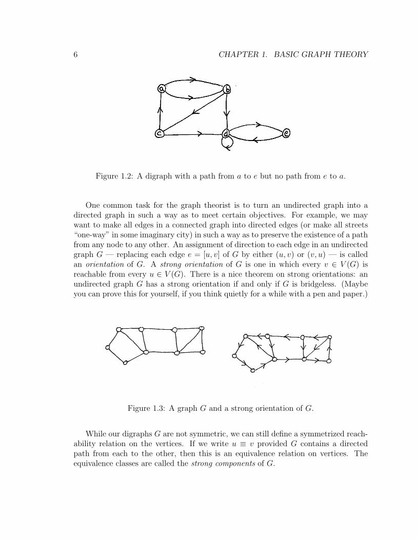
Figure 1.2: A digraph with a path from a to e but no path from e to a.

One common task for the graph theorist is to turn an undirected graph into adirected graph in such a way as to meet certain objectives. For example, we maywant to make all edges in a connected graph into directed edges (or make all streets“one-way” in some imaginary city) in such a way as to preserve the existence of a pathfrom any node to any other. An assignment of direction to each edge in an undirectedgraph G — replacing each edge e = [u, v] of G by either (u, v) or (v, u) — is calledan orientation of G. A strong orientation of G is one in which every v ∈ V (G) isreachable from every u ∈ V (G). There is a nice theorem on strong orientations: anundirected graph G has a strong orientation if and only if G is bridgeless. (Maybeyou can prove this for yourself, if you think quietly for a while with a pen and paper.)

Figure 1.3: A graph G and a strong orientation of G.

While our digraphs G are not symmetric, we can still define a symmetrized reach-ability relation on the vertices. If we write u ≡ v provided G contains a directedpath from each to the other, then this is an equivalence relation on vertices. Theequivalence classes are called the strong components of G.

1.2. COLORING AND FLOWS 7

Figure 1.4: A graph with a bridge admits no strong orientation.

Figure 1.5: A digraph with three strong components.

1.2 Colorings and nowhere-zero flows

The Four-Color Conjecture, stated in 1852 and solved in 1976, has captured theimagination of many students of mathematics. It states that every subdivision of theplane into regions by piecewise linear boundaries has its regions colorable by at mostfour colors in such a way that any two regions with a common boundary of positivelength are colored with different colors. While the Four Color Theorem (or “4CT”)has no natural practical application, the century-long search for a solution to thisproblem generated perhaps the bulk of the theory of graphs, and this has turned outto have great value in the solution of many other problems.

In spite of the esoteric nature of the 4CT, more general graph coloring prob-lems have many practical applications and scientists continue to search for efficient


algorithms to color graphs. In this lecture, we will content ourselves with a briefdescription of the problems and one application.

A vertex coloring is a coloring of the vertices of a graph in which adjacent verticesalways get different colors. Let G = (V, E) be a finite undirected simple graphand let C be a set of objects which we will call “colors”. (While ‘fire engine red’,‘hunter green’, ‘charcoal’ and ‘chartreuse’ would be more imaginative, we typicallyuse C = 1, 2, . . . , k when k colors are in play.) A proper vertex coloring (or, simply,a “coloring” when no confusion is risked) of G with colors in C is a function

c : V → C

satisfying c(u) 6= c(v) whenever [u, v] is an edge of G.

Figure 1.6: A bipartite graph is one whose vertices can be colored with two colors.

A graph G is bipartite if its vertices can be colored with two colors. An exampleis given in Figure 1.6. It is not hard to prove that a graph G is bipartite if and onlyif G has no cycles with an odd number of edges. Bipartite graphs arise frequently indiscrete optimization, such as the problem of optimal assignment of workers to tasksor the transshipment problem.

In the classic map-coloring problem, the graph to color is not the configuration ofboundaries, but rather an abstract construct in which the regions become the verticesand adjoining regions are connected by an edge.

1.2. COLORING AND FLOWS 9

But the most prevalent application of graph coloring today is in scheduling prob-lems. In the simplest form, we have a graph where each vertex is an event which mustbe scheduled. Two events which cannot be scheduled at the same time are joined byan edge. The “colors” in this scenario are the possible time slots for the events.

For example, suppose we have a university at which final examinations must bescheduled. (At many universities, these 3-hour exams are scheduled over a ten-dayperiod, separated from the end of term by a one-week study period.) Two courseswhich have a student in common cannot be scheduled at the same time (in the idealscenario) and so the students give us the edges in a graph defined on the set of coursesas vertices.

A more complicated problem (and quite a challenging one in practice) is coursescheduling for a university (or project scheduling at a factory). A full solution tothis problem assigns to each section of each course not only a time slot, but a set ofstudents, a professor, and a room. Various constraints — such as room size, audio-visual capabilities and handicapped accessibility, instructor expertise and preference,and student schedules — add a complex system of edges to this graph. Rarely isa proper coloring available and the optimization problem becomes one in which thenumber of conflicts is to be minimized. Different universities handle this in differentways.

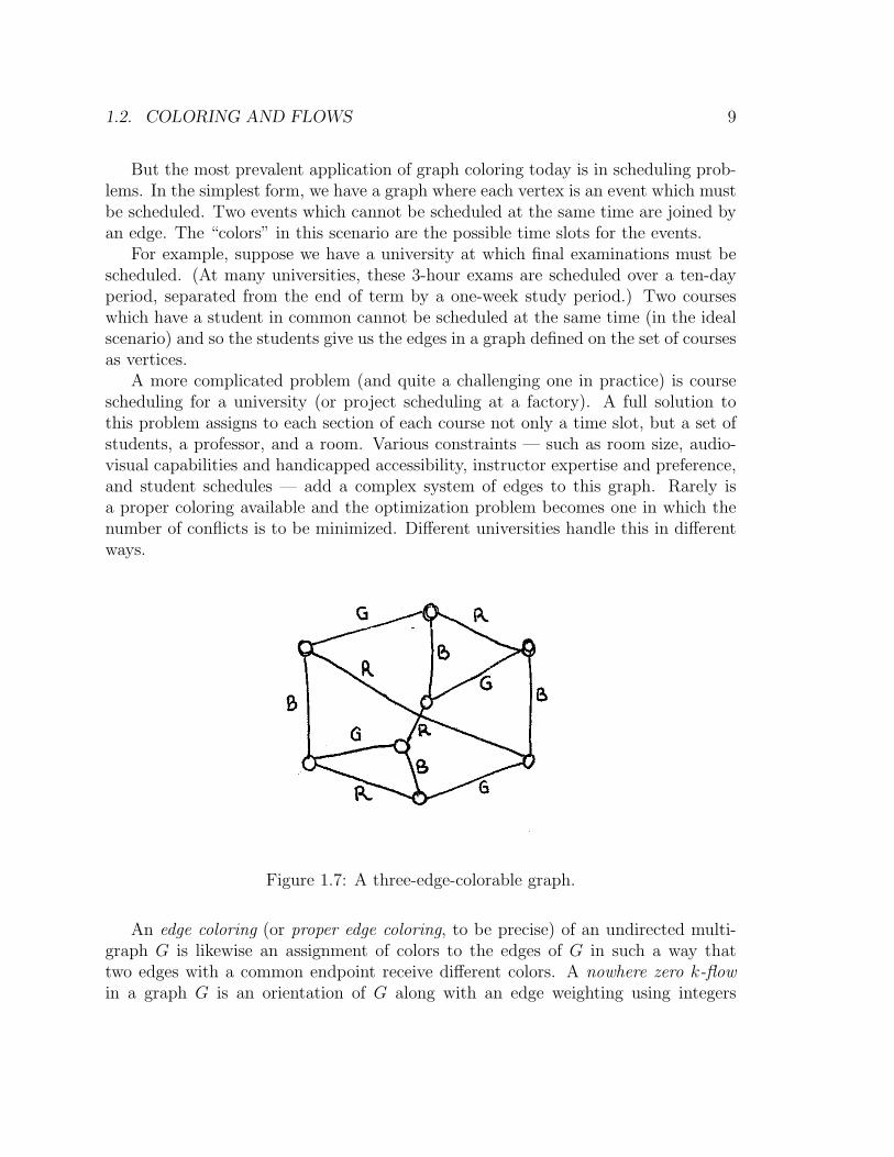
Figure 1.7: A three-edge-colorable graph.

An edge coloring (or proper edge coloring, to be precise) of an undirected multi-graph G is likewise an assignment of colors to the edges of G in such a way thattwo edges with a common endpoint receive different colors. A nowhere zero k-flowin a graph G is an orientation of G along with an edge weighting using integers


1, 2, . . . , k− 1 which satisfies conservation of flow at every vertex: the total weightof the arcs going into node u matches exactly the total weight of the arcs going outof node u. For example, the graph of the 3-cube admits a nowhere zero 3-flow, butthe famous Petersen graph (with ten vertices, all of degree three, and no cycles oflength less than five) does not. (It does not even admit a nowhere zero 4-flow.)

Figure 1.8: The Petersen graph is not three-edge-colorable; also, the graph admitsno nowhere zero 4-flow.

1.3 Factors in graphs

Let’s finish this section with a survey of substructures in graphs. A matching in agraph is a collection of edges no two of which share a common vertex. For example, ina bipartite graph G = (V, E) where the vertices are partitioned into two color classesV = W ∪ T (“workers” and “tasks”) and every edge joins one element of W to oneelement of T , a matching represents an assigment of some subset of the workers tosome subset of the tasks in such a way that each worker is assigned to at most onetask and each task is matched to at most one worker. (For obvious reasons, problemsof this sort are sometimes called “marriage problems”, but I won’t conjecture whichgender more resembles the set of tasks here.) Let G = (V, E) be a graph and letM ⊆ E be a matching. We say M saturates u ∈ V if u is the end of some edgebelong to M ; an “unsaturated” vertex is one which is incident to no edge of the

1.3. FACTORS IN GRAPHS 11

matching. A perfect matching in a (not necessarily) bipartite graph G is a matchingwhich saturates all vertices. The task of finding a perfect matching in a given graphG — or a maximum weight matching in a weighted graph (G, w) — is a challengingcomputational task that we will address later in the course.

In a graph G = (V, E) with n vertices, a Hamilton cycle1 is a cycle which visitsevery vertex; i.e., a cycle of length n in G. We view such a cycle as a subset Cof the edge set E. Note that if C is a Hamilton cycle, then every vertex in thesubgraph H = (V, C) has degree two but, except when G is small, G typically containsmany other “2-regular” spanning subgraphs. Among these, the Hamilton cycle isdistinguished by the fact that it alone is connected. As an example, consider thePetersen graph. With a bit of work, one is easily convinced that this graph does nothave a Hamilton cycle; but if we delete any vertex whatsoever, the resulting graph onnine vertices does admit such a cycle. So the Petersen graph is not Hamiltonian, butany subgraph of it having 9 vertices and 12 edges is Hamiltonian: all such subgraphscontain a Hamilton cycle.

Let (G, w) be a weighted undirected graph with edge weights w : E → R. Thetravelling salesman problem (or “TSP”) for (G, w) is to find a Hamilton cycle in Gof minimum total weight: H = (V, C) is a Hamilton cycle and, among such, w(C)is as small as possible. This problem is extremely hard to solve in practice, yet isclosely related to a number of problems of practical importance such as the vehiclerouting problem. Since many graphs do not admit even a single Hamilton cycle, it isattractive to formulate all travelling salesman problems as problems on a completegraph.

The complete graph Kn is a simple undirected graph on n vertices with(

n2

)edges,

one joining each pair of distinct nodes. By allowing +∞ as an edge weight, we canreformulate the TSP (or the Hamiltonicity question) on any graph with n nodes asan equivalent TSP on Kn. We can also consider the Hamilton cycle problem andTSP on directed graphs, and this reduction to the (directed) complete graph worksin much the same way for these.

A k-factor in a graph G is a spanning subgraph in which every vertex has degreeexactly k. Of course, a graph having any vertex of degree less than k contains nok-factor. For example, a 1-factor in G is the same as a perfect matching in G anda Hamilton cycle in G is an example of a 2-factor in G, but not all 2-factors areHamilton cycles (consider, for example, two disjoint cycles of length four in the 3-cube). A 2-factor is equivalent to a collection of cycles in the graph which, combined,pass through every vertex exactly once. A Hamilton cycle occurs as the special caseof a single cycle achieving this effect: it is a connected 2-factor.

1These are named in honor of the Irish mathematician and physicist Sir William Rowan Hamiltonwho, in 1857, invented a game – the Icosian Game – based on finding such cycles in graphs.


Figure 1.9: A 1-factor is also called a “perfect matching”.

To achieve more versatility (and, hence, address a wider array of applications),we generalize the above notion to a b-factor. Let b : V → Z be an integer-valuedfunction on the vertex set V of a graph G. A b-factor in G is a spanning subgraphH = (V, S) in which each vertex u ∈ V has degree exactly b(u). Clearly, if b(u) < 0 orb(u) > deg(u) (the degree of vertex u) for any u ∈ V , then no such subgraph exists.But non-existence conditions beyond this get harder and harder to find. So we alsohave on our plate the task of finding good algorithms to find b-factors in graphs andminimum/maximum weight b-factors in weighted graphs.

1.4 The Menagerie

At the end of each chapter in these notes, we will describe one or more discreteoptimization problems for which we present no solution. These problems may become from applications or may simply be exotic puzzles related to the material inthe chapter. We have three reasons to include such problems. First, it is importantfor the student to see that not all problems are neatly described in terms of graphsor matrices; such a formulation often requires one to be creative or to simplify theproblem. Second, a text can often give the impression that “all of the answers areknown”, that there is no room left for mathematical research. (On a related note, itis amazing how many students complete freshman calculus erroneously believing thatformulas for antiderivatives are known for all algebraic functions.) Finally, it is good

1.4. THE MENAGERIE 13

Figure 1.10: This graph has a b-factor for the values b(u) given at its nodes.

to leave a few open problems in order for the talented student to try out her/his skillat discovering — and verifying the correctness of — algorithms.

The optimal design of parking lots is an important and complex problem in indus-try. The designer must consider a multitude of issues, including traffic flow, pedestrianpatterns, and zoning rules such as number of trees to be planted per 10,000 squarefeet of pavement. A designer can also make aisles (typically 24 feet wide at minimum)narrower by allowing only one-way traffic or placing parking spaces at an angle. (Butthen these spaces need to be larger than the standard ones.) We describe only thesimplest version of this problem, ignoring all these issues as well as entrance and exitlocations.

Parking Lot Planning: Maximize the number of parking spaces in a given polygonalregion.Input: A polygonal region in the plane.Goal: Maximize the total weight of a legal configuration of rectangles in the region.A rectangle 36× 8.5k has weight (value) 2k and a rectangle 18× 8.5k has weight k.An arrangement of rectangles is “legal” if no two points in distinct rectangles are lessthan 24 units apart.

When raking leaves, one does not wish to rake the same area twice. Leavesare gathered into piles which are later gathered up by one’s children. The optimallocation of these piles depends on the density of leaves across the region: one does


not wish to transport large amounts of leaves over long distances. We simplify thisproblem in what, at first, seems a ridiculous way. We assume that there are a smallnumber, n, of leaves and an even smaller number, k, of leaf-pile locations. Since wecan approximate the density by a bunch of points marking the centers of “clumps”,this is not such a bad approximation.

Raking Leaves: Minimize the amount of raking to move n leaves in the unit squareinto k piles.Input: A set L of n pairs (xi, yi) of points inside the unit square [0, 1]× [0, 1].Goal: Find a set P of k points in [0, 1] × [0, 1] and a function f : L → P such thatthe raking distance

∑`∈L d(`, f(`)) is minimized. (Here, d(·, ·) is Euclidean distance

in the plane.)

Exercises

Exercise 1.4.1. Prove that if there is a walk from u to v in graph G, then there is apath from u to v in G.

Exercise 1.4.2. Prove that a graph on n vertices with no cycles has at most n − 1edges. (Note that loops form cycles of length one and parallel edges between a pair ofvertices lead to cycles of length two.)

Exercise 1.4.3. Is it possible to have exactly one cut vertex? Is it possible that everyvertex in graph G is a cut vertex? How about “all but one”?

Exercise 1.4.4. Prove:∑

v deg(v) = 2|E(G)| where the sum is over all v ∈ V (G).What is the analogous identity for directed graphs?

Exercise 1.4.5. Use the result of the previous exercise to prove the HandshakingLemma: In any undirected simple graph, the number of vertices of odd degree isalways even.

Exercise 1.4.6. What is the maximum number of edges in a non-Hamiltonian simplegraph on six vertices?

Exercise 1.4.7. Find the smallest non-bipartite graph that contains no cycles oflength three.

Exercise 1.4.8. Prove that every Hamiltonian graph has a strong orientation.


Exercise 1.4.9. The n-prism is a graph on 2n vertices formed by taking two copies ofa cycle of length n (call these the “inside cycle” and “outside cycle”) and joining eachvertex on the inside cycle by a new edge to its corresponding vertex on the outsidecycle. Find an orientation of the 8-prism having strong components of sizes exactly6, 4, 4, 1 and 1.

Exercise 1.4.10. Find a nowhere zero 4-flow in the graph of Figure 1.7.

Exercise 1.4.11. For the graph in Figure 1.9, find a function b on vertices satisfying0 ≤ b(v) ≤ deg(v) for all vertices v such that no b-factor exists.


e

Two

Trees and the Greedy Algorithm

Nov. 1, 2012

Today we discuss trees and present the “greedy method” for finding a minimumcost spanning tree. Trees are important for several reasons, but mainly because atree is, in a sense, the simplest or cheapest way to connect up a bunch of nodes in anetwork. So we repeatedly find ourselves needing them, and needing them in a hurry.

The graphs we discuss today will all be undirected. A graph is acyclic if it containsno cycles. If u and v are vertices in an acyclic graph G and v is reachable from u,then there is exactly one path in G from u to v. (If there were two or more distinctpaths, then the union of two of these paths would contain a cycle. Think about this.)An undirected acyclic graph is called a forest. Naturally, a forest consists of a bunchof trees. A tree is a connected acyclic undirected graph. So each component of aforest is a tree. An example appears in Figure 2.1.

Figure 2.1: A forest with four components. Each component is a tree.

17

18 CHAPTER 2. TREES AND THE GREEDY ALGORITHM

Lemma 1. In a connected simple graph on n vertices, every spanning tree containsexactly n− 1 edges. Any spanning subgraph with fewer than n− 1 edges is necessarilydisconnected; any subgraph including n or more edges must contain a cycle.

Let G = (V, E) be a graph and let H = (W, S) be a subgraph of G. We say H is aspanning subgraph of G if W = V ; i.e., H includes all the vertices of G, but perhapsnot all the edges. For example H = (V, ∅) is a spanning subgraph of G = (V, E)with no edges and |V | components of size one. This trivial spanning subgraph isthe starting point of our greedy algorithm. We want to judiciously add edges to thisedge-less subgraph until we arrive at a “best” spanning tree of G; i.e., a spanningsubgraph which is a tree.

By a weighted graph (or “edge-weighted graph”) we mean an ordered pair (G, w)where G = (V, E) is an undirected graph and w : E → R is a real-valued function onthe edges. The Minimum Spanning Tree (MST) problem is to find a spanning tree ina given weighted graph having smallest possible total weight.

If H = (W, S) is a subgraph of graph G = (V, E) with edge weights w, then theweight of H is given by

w(H) =∑e∈S

w(e).

Our goal here is to find, in G, a spanning tree T = (V, S) with the property that

w(T ) ≤ w(T ′)

for any other spanning tree T ′ in G.

2.1 The greedy algorithm

Here is our first algorithm to solve this problem: the “greedy algorithm”.

Kruskal’s Algorithm

Input: Weighted graph (G, w) with G = (V, E)Output: Either a subset S ⊆ E such that T = (V, S) is a minimum weight spanningtree in G or a report that G is disconnected.

Description: Let n = |V | and m = |E|. As a pre-processing step, first sort theedge set E from lowest to highest weight. In other words, write

E = e1, e2, . . . , em

so thatw(e1) ≤ w(e2) ≤ · · · ≤ w(em).

2.1. THE GREEDY ALGORITHM 19

Now initialize S = ∅ and consider the edges in turn, from e1 up to em, examining eachedge once. When considering edge ek = [u, v], we ask if the current forest F = (V, S)already contains a path from u to v. If so, we reject this edge; if not, then weaccept this edge and augment S to S ∪ ek.

If we ever reach |S| = n − 1, we stop and give T = (V, S) as our spanning tree.If we finish examining all edges and |S| < n− 1, then we report that the graph G isnot connected.

Sometimes when we present an algorithm in English, the devil is in the details.Here, we have left to the reader the issue of deciding whether or not the current forestF = (V, S) at some point in the algorithm contains a path from some node u toanother node v. One way to improve this “component management” is to intuitivelyhave each component elect a “leader node” for that component. Then, when edgese = [u, v] is considered, we can ask whether the components currently containing uand v have the same leader node. If so, then each is reachable from the other and theedge e is rejected; if not, then the edge is accepted and we then have the problem ofefficiently updating the leader node.

One way to do this is to let the vertex set be identified with the first few positiveintegers, V = 1, 2, . . . , n, and to define the “leader node” of a component to be thesmallest vertex in that component (in the natural ordering of integers). Then, wecan define a function up(v) which is initialized to up(v) = v for all nodes v. Whenan edge e = [u, v] is added into S, we look at the larger of the two leader nodes,say up∗(v) ≥ up∗(u), and update up(up∗(v)) to be equal to up(u). Then, when welater wish to find the leader node of this component, we start at a node v0 = vand iterate vh+1 := up(vh) until we reach a limit, up∗(v0) = up(vh) = vh, which willhold only when vh is the smallest node in its component. (This still allows room forimprovement; periodic “tree balancing” can help us avoid too many iterations of thisup function.)

The correctness of this algorithm hinges on several basic properties of trees, whichwe now present.

Lemma 2. Let G = (V, E) be a finite connected undirected graph and let T = (V, S)be a spanning subgraph of G. Then any two of the following properties imply the third:

• T is acyclic

• T is connected

• T has |V | − 1 edges.

Conversely, if T is a spanning tree of G, then all three of these properties hold.


Proof: Exercise.

The next lemma is sometimes called the “Exchange Axiom” since it plays a rolein the definition of a matroid.

Lemma 3. Let G = (V, E) be a connected undirected graph and let T = (V, S) be aspanning tree in G. If e is any non-tree edge (i.e., e ∈ E − S), then the subgraph

T + e := (V, S ∪ e)

contains exactly one cycle. Moreover, if e′ is any edge of this cycle, then the subgraphT ′ = (V, (S ∪ e)− e′) is also a spanning tree.

Proof: Exercise.

As an example, we briefly summarize the progress of Kruskal’s algorithm in Figure2.2.

Figure 2.2: Given this graph, the greedy algorithm chooses edges [b, c], [c, e], [d, h],[g, j], [a, b], [c, g], [e, h], [f, i] and [c, f ] rejecting, along the way, edges [b, e] and [a, d].

Now we prove that the greedy algorithm performs as promised. As in the descrip-tion of the algorithm, let the edge set E = e1, . . . , em be ordered so that

w(e1) ≤ w(e2) ≤ · · · ≤ w(em)

2.2. PRIM’S ALGORITHM 21

and let T ′ = (V, S ′) be the spanning tree produced by Kruskal’s algorithm. LetT = (V, S) be any other spanning tree in graph G and let ej be chosen so that

j := minh : eh ∈ S − S ′.

We ask why the greedy algorithm did not choose edge ej. Of course, the edge wasrejected because its introduction would have created a cycle when added to the forestexisting at iteration j of the method. But then — aside from edge ej itself — thiscycle consists only of edges from the set e1, . . . , ej−1. And all of these edges eh

enjoy the property that w(eh) ≤ w(ej). Since T does not contain a cycle, there mustbe some edge ei in this cycle (i 6= j) which does not belong to T . So build a new treeT ′′ from T ′ by replacing edge ei with edge ej. By the above lemma, this is again aspanning tree. Since w(ej) ≥ w(ei), we have w(T ′′) ≥ w(T ′). And T ′′ has one moreedge in common with T than does our greedily-constructed tree T ′. Repeating thisexchange process, we obtain a sequence of spanning trees

T ′, T ′′, T ′′′, . . .

each one having more edges in common with T than the previous one and havingweights

w(T ′) ≤ w(T ′′) ≤ w(T ′′′) ≤ . . .

Since T has finitely many edges, we eventually arrive at T and this string of inequal-ities gives us w(T ′) ≤ w(T ) as claimed.

2.2 Prim’s Algorithm

In certain applications, it is natural to build a spanning tree starting from some rootvertex so that the edges chosen so far at any point in the algorithm induce a connectedacyclic subgraph.

Prim’s Algorithm

Input: Weighted graph (G, w) with G = (V, E) and r ∈ VOutput: Either a subset S ⊆ E such that T = (V, S) is a minimum cost spanningtree in G or a report that G is disconnected.

Description: Initialize U = r and S = ∅. As long as there is an edge with oneend in U and one end in U = V − U ,

• find the smallest weight edge e = [u, v] with one end u ∈ U and the other, v, inU


• Update S to S ∪ e

• Update U to U ∪ v

It is fairly clear that the algorithm produces a forest T = (V, S) with |S| = |U |−1.If Prim’s algorithm terminates with U 6= V , then there are no edges between U andU and G contains no spanning tree. But when graph G is connected, this algorithmcan be shown to produce a spanning tree of minimum total weight. The proof is leftas an exercise.

Prim’s algorithm must also be implemented with careful thought. Heineman,Pollice and Selkow note that a priority queue is the natural choice of data structureto maintain a list of vertices not yet in the tree, together with a regularly updatedmeasure of the smallest weight edge from each vertex to a vertex in U . They thenpoint out that, since all nodes are initially in the “queue” and no node is ever addedback into the queue, a binary heap data structure will suffice for this application.

2.3 The Menagerie

Let us instead consider instead a directed graph G = (V, A) on n vertices and ask“what is the directed analogue of a spanning tree?” There are two possible answershere.

An arborescence in G with root r ∈ V is a set S ⊆ A of n− 1 arcs in G such thatthe subgraph (V, S) contains a unique directed path from node r to any other nodein G. Given a weighted directed graph G with edge weights w and a node r ∈ V , wemay ask for a minimum weight arborescence rooted at r.

A digraph G is strongly connected if it contains a directed path joining any nodeto any other. (So G is strongly connected if and only if it contains an arborescencerooted at r for every vertex r ∈ V .) A natural question to ask is how to join upall of these pairs of vertices in the cheapest possible way. Given that G is stronglyconnected, we may ask for a minimum weight subgraph with the property that thissubgraph contains a directed path from any node r to any node t in G. This is reallya different problem from the arborescence problem; while an arborescence containsexactly n − 1 arcs, we do not know how many arcs belong to the optimal subgraphin this case.

We finish with a combinatorial game. In the Shannon switching game, a graphand a pair of nodes X and Y in that graph are specified. Two players Short andCut take turns choosing edges from the graph. Edges chosen by Short are foreversecured and cannot thereafter be deleted; edges chosen by Cut are delete and cannotbe subsequently secured. If, at some point, the subgraph secured by Short contains


a path from X to Y , Short wins. On the other hand, if at some point the graphbecomes disconnected, with X and Y in different components, then Cut wins.

Figure 2.3: Can you find a minimum weight strongly connected subgraph in thisdigraph?

Exercises

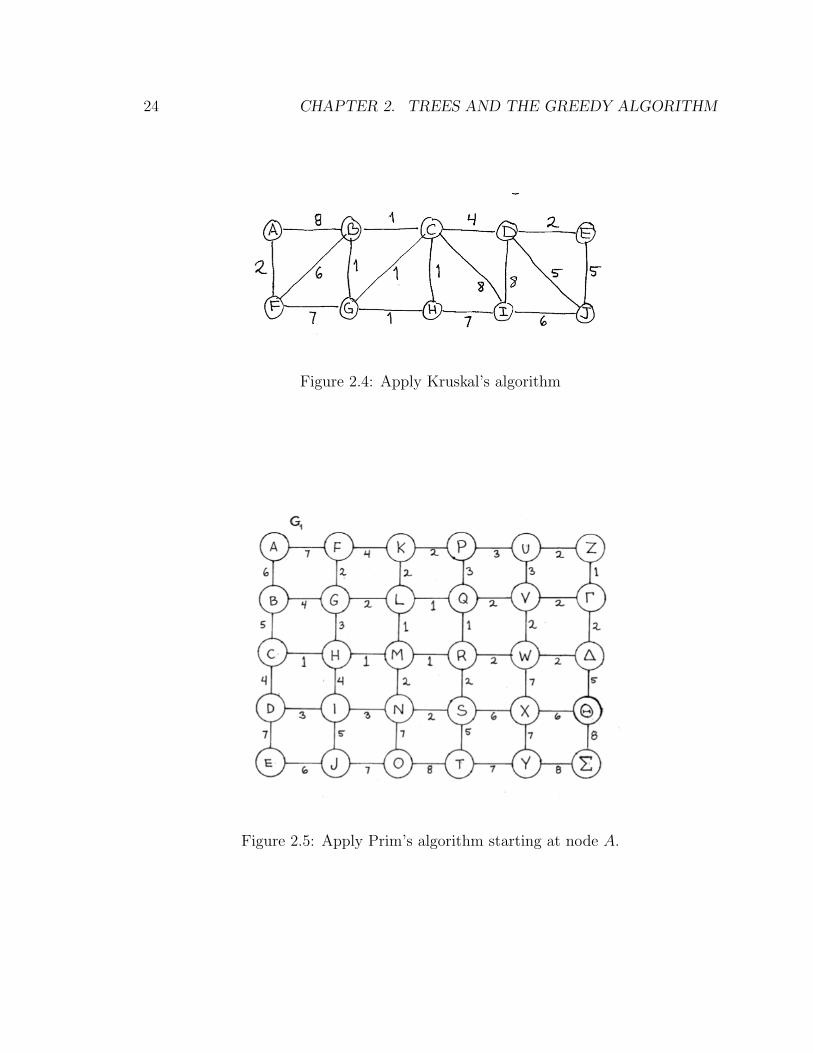
Exercise 2.3.1. Apply Kruskal’s algorithm to find a minimum cost spanning tree inthe graph in Figure 2.4.

Exercise 2.3.2. Apply Prim’s algorithm, starting from node A, to find a minimumcost spanning tree in the graph in Figure 2.5.

Exercise 2.3.3. Consider once again Shannon’s switching game. A well-known the-orem states that, if G contains a pair of edge disjoint spanning trees, then for anyvertices X and Y in the graph, Short has a winning strategy. So who wins for thevarious choices of X and Y in the graph of Figure 2.6?


Figure 2.4: Apply Kruskal’s algorithm

Figure 2.5: Apply Prim’s algorithm starting at node A.


Figure 2.6: Play Shannon’s switching game.

Three

Basic Search Trees

Nov. 6, 2012

Today we discuss a generic search algorithm for a connected undirected graph andshow how it specializes to the famous “breadth-first search” and “depth-first search”algorithms in computer science.

Let us use the informal term “bag” to mean simply a set. We will later comparetwo ways to move items in and out of our “bag”.

3.1 Generic Search

Generic Search Algorithm

Input: Connected graph G = (V, E) with root node rOutput: A subset S ⊆ E such that T = (V, S) is a spanning tree in G.

Description: Start with S = ∅. Throughout the algorithm, vertices will be splitinto three groups: “exhausted” vertices, vertices in the bag, and unvisited vertices.Initially, only the root node r is in the bag and all other vertices are marked “unvis-ited”.

As long as there is something in the bag, do the following:

• consider some node u in the bag

• see if there is an edge e = [u, v] such that v is unvisited

• if so

– put the edge e into the tree: augment S to S ∪ e26

3.2. BREADTH-FIRST AND DEPTH-FIRST SEARCH 27

– put v into the bag

• if there is no such edge e, then mark vertex u as “exhausted” and move u outof the bag.

This algorithm gives the computer programmer a great deal of freedom in imple-mentation. Many choices need to be made and these choices achieve different desiredeffects. But, in any case, we can prove that the algorithm does indeed return a span-ning tree when applied to a connected graph G. Every time a node v is moved intothe bag, the number of edges in S increases by one. We claim that every node otherthan the root r gets moved into the bag at some point and this gives |S| = |V | − 1.Moreover, when a node v is moved into the bag, the current subgraph (V, S) containsa path from v to the root r (why?) and so the algorithm ends with a connectedsubgraph having |V | − 1 edges. By Lemma 1, this subgraph is a spanning tree.

Now suppose, by way of contradiction, that some vertex v 6= r never enters thebag. Let’s look at the set W of vertices which at some point are in the bag. (In class,I called this bag F , but that is not important.) Since we are assuming that W 6= Vand that the graph is connected, there exist vertices w, x with the property thatw ∈ W , x 6∈ W and [w, x] is an edge. Now examine the point in the algorithm wherenode w is declared to be exhausted. At this point, x must be labelled “unvisited”and therefore the edge e = [w, x] is considered by the algorithm and accepted into thetree, thereby moving x into the bag. This contradicts our assumption that x 6∈ W .

3.2 Breadth-first and depth-first search

Now we see what happens when the “bag” is implemented as a queue. A queue isa “first-in-first-out” (or FIFO) data structure that implements a set. If we view theelements in a queue as ordered horizontally, from left to right, an element is alwaysadded at the right (at the “end of the line”) and when we consider, or remove, anelement from the queue, we always choose the leftmost member.

Breadth-First Search (bfs) Algorithm

Input: Connected graph G = (V, E) with root node rOutput: A subset S ⊆ E such that T = (V, S) is a breadth-first search tree rootedat r in G.

Description: Start with S = ∅. Initially, only the root node r is in the queue andall other vertices are marked “unvisited”.

As long as the queue is non-empty, do the following:

• consider the first node u in the queue

28 CHAPTER 3. BASIC SEARCH TREES


• if so

– put the edge e into the tree: augment S to S ∪ e– put v into the end of the queue

• if there is no such edge e, then mark vertex u as “exhausted” and move u outof the queue.

We have already proved above that this algorithm produces a spanning tree. Thissort of tree has some special properties. We may partition the vertex set into “layers”L0, L1, L2, . . . as follows. Initialize L0 = r and Lk = ∅ for k > 0. When an edgee = [u, v] is moved into S, one end of e — node u, say — is already in the queue andbelongs to some layer Li. So we put the other end v into layer Li+1. In this manner,each node of the connected graph G ends up in a unique set Lk and the Lk form apartition of set V .

Lemma 4. Let G = (V, E) be a connected undirected graph, let r ∈ V , and letT = (V, S) be the breadth-first search spanning tree rooted at r in G. Then

• if node v in G belongs to layer Lk, then the shortest (r, v)-path in G (in termsof number of edges) has length k and one such path is the unique (r, v)-path inT .

• every non-tree edge in G joins vertices in the same layer Lk or in consecutivelayers Lk and Lk+1.

Proof: The first part follows by induction. Of course, there is a path with zero edgesfrom r to r and L0 contains only r. If e = [u, v] is entered into S and v is entered intothe queue, then the tree at this point contains a path of length one from u to v. Byinduction, we assume that u ∈ Lk for some k and that the tree contains a shortestpath from r to u of length k. Appending edge e to this path gives a path of lengthk + 1 from r to v and we do indeed have v ∈ Lk+1.

Now suppose that v is a vertex in some layer Lk and G contains and (r, v)-pathusing less than k edges. Among such vertices, let’s focus on one for which k is assmall as possible.

r = u0, e1, u1, e2, u2, . . . , e`, u` = v

is a path from r to v of length ` < k, then the subpath

r = u0, e1, u1, e2, u2, . . . , e`−1, u`−1

3.2. BREADTH-FIRST AND DEPTH-FIRST SEARCH 29

is a path from r to v′ := u`−1 of length ` − 1. By minimality of k, we must havev′ ∈ L`−1. But `− 1 is less than k and so our examination of node v′ would considerthe edge e = [v′v] forcing v into L` and not Lk, a contradiction.

Now the last part of the proof follows since any non-tree edge e = [u, v] can beappended to a shortest path from r to u (or r to v, if v is closer to the root) to get apath from r to v (resp. to u). If u ∈ Lk and v ∈ L`, we have without loss of generalityk ≤ `. So there is a path of length k from r to u and this yields a path of lengthk + 1 from r to v. Since ` is the minimum number of edges in a shortest (r, v)-path,we have k ≤ ` ≤ k + 1.

Next, we consider implementing our generic bag as a “stack”. A stack is is a “last-in-first-out” (or LIFO) data structure that implements a set. If we view the elementsin a stack as piled vertically, from bottom to top, an element is always added at thetop and when we consider, or remove, an element from the stack, we again choosethe top element.

Depth-First Search (dfs) Algorithm

Input: Connected graph G = (V, E) with root node rOutput: A subset S ⊆ E such that T = (V, S) is a depth-first search tree rooted atr in G.

Description: Start with S = ∅. Initially, only the root node r is on the stack andall other vertices are marked “unvisited”.

As long as the stack is non-empty, do the following:

• consider the top node u on the stack


• if so

– put the edge e into the tree: augment S to S ∪ e– push v onto the top of the stack

• if there is no such edge e, then mark vertex u as “exhausted” and move (or“pop”) u off the stack.

Again, our proof for the generic case shows that this algorithm produces a span-ning tree. This sort of tree has its own special properties. We define an “ancestor”relation on V : say that node u is an ancestor of node v if u lies on the unique (r, v)-path in our DFS tree T . So, for example, each node is an ancestor of itself and r isan ancestor of v for every v since G is connected.


Lemma 5. Let G = (V, E) be a connected undirected graph, let r ∈ V , and letT = (V, S) be the depth-first search spanning tree rooted at r in G. Then

• when a node u is marked “exhausted” by the algorithm, every node having u asan ancestor is also exhausted;

• every non-tree edge in G joins some vertex v to an ancestor u of that vertex.

Proof: Exercise. In Figure 3.1, we give a sketch of a graph and in Figure 3.2, we give the two

search trees that our algorithms produce from this graph. In order to get a well-defined answer, we adopt the following convention. When a query is made to thedata structure describing a graph, such as “Give me an edge with endpoint u”, theedge e = [u, v] with node label v smallest is returned first. The next time we makethe same query, the second smallest possible v is chosen, and so on. We adopt thisconvention in the exercises below.

Figure 3.1: A graph to be searched efficiently. Use 1 as root node.


Figure 3.2: Depth-first and breadth-first search trees based at root node 1 for thegraph in Figure 3.1.

3.3 The Menagerie

Efficient search is a ubiquitous problem in computing. Every day, various businessesare looking for more efficient ways to search graphs, to search the world-wide web,to search databases. There is a substantial literature on all these topics. So we canwander off in any number of directions with our excursion here.

An interval graph is a graph each of whose vertices vi is identified with some inter-val [ai, bi] on the real number line. Adjacency is defined by non-empty intersection:vi is adjacent to vj if the intervals [ai, bi] and [aj, bj] have a point in common. In thiscase, can you find a more efficient way to visit every vertex than using DFS or BFS?

Exercise 3.3.1. Find breadth-first and depth-first search trees in the graph of Figure3.3, starting at vertex 1.

Exercises

Exercise 3.3.2. Homework problems go here, eventually.


Figure 3.3: Compute BFS and DFS trees. Use 1 as root node.

Four

Shortest Path Problems

Nov. 8, 2012

In today’s class, we look at the problem of finding the shortest path in a weighteddirected graph from a specified origin to a specified destination. We also look at somevariations on this problem without giving algorithms for their solution.

4.1 The Landscape of Problems

A path from node r to node t in a graph G = (V, E) (or a digraph G = (V, A)) is asequence

P : r = u0, e1, u1, e2, u2, . . . , ek, uk = t

which alternates between vertices ui and edges/arcs ei+1 in such a way that

• ei = [ui−1, ui] in the undirected case (ei = (ui−1, ui) in the directed case);

• the vertices u0, . . . , uk are all distinct.

In a weighted graph or digraph, we aim to find a path from a node r to a node t ofminimum total weight. So we have a weight function w : E → R on edges E (or onarcs, A, in the directed case) and we wish to minimize the length or weight of thepath

w(e1) + w(e2) + · · ·+ w(ek).

There are a number of choices one must make in clearly defining a shortest pathproblem:

• Is the graph directed or undirected?

• Is the graph finite or infinite?

33

34 CHAPTER 4. SHORTEST PATH PROBLEMS

• Do we allow negative edge weights?

• Do we allow negative-length cycles?

• Do we seek shortest paths between all pairs of vertices? From one vertex to allothers? Or just from one origin r to one destination t?

• Do we need only one path between r and t or would we prefer to find all suchpaths of shortest length?

• Do we insist on a correct answer or are we willing to allow some probabilitythat the path found is not shortest or that no path is found even if one exists?

The various answers to these questions lead to a range of algorithms and to subprob-lems of varying hardness. The first algorithm we explore is the most important one.Dijkstra’s algorithm, published in 1959, takes as input a weighted finite digraph withnon-negative arc weights and a root node r. For this digraph, the algorithm findsshortest paths from r to all nodes reachable from r. This algorithm is easily seento work for the undirected case; other extensions will be discussed after we give itsproof of correctness.

4.2 Dijkstra’s algorithm

One of the most popular algorithms in computer science, used in many industries,many times a day (perhaps even millions of times per second, if we combine internetpacket routing and GPS systems), is Dijkstra’s algorithm for shortest paths.

The algorithm, in its simplest form, works on a digraph with a root node r andcomputes shortest paths from r to all other vertices reachable from r. We assumethat all edge weights are non-negative. The algorithm also works just fine on anundirected graph if we replace each edge [u, v] by the two arcs (u, v) and (v, u). Inmany applications, we seek only a shortest path from r to a single node t in thedigraph; in this case, we can easily stop the algorithm when t becomes “permanentlylabelled” (as defined below).

In our view of Dijkstra’s algorithm, we maintain a laminar partition of the vertexset; in digraph G = (V, A), we have

V = P ∪ F ∪ U ,

a disjoint union of three sets: the “permanent” set P , the “frontier” F , and the“unvisited” set U . At each iteration, one node moves from the frontier F to thepermanent set P and this is repeated until all nodes are in P (or, in the single-pathcase, the target vertex t belongs to P).

4.2. DIJKSTRA’S ALGORITHM 35

Figure 4.1: Conceptual diagram of vertex partition in Dijkstra algorithm.

The algorithm constructs a shortest path tree T rooted at a node r. This treeincludes a shortest path from r to every node in the digraph which is reachable fromr.

Dijkstra’s Algorithm

Input: Digraph G = (V, A) with arc weights w : A → R and root node rOutput: A shortest path tree rooted at r together with a length function `(v) whichgives the length of a shortest path in G from r to v for every node v ∈ V reachablefrom r.

Description: Start with

P = ∅, F = r, U = v ∈ V |v 6= r .

Define `(r) = 0 and `(v) = +∞ for each v 6= r. Initially, pred(v) is undefined for eachvertex v.

As long as the frontier F is non-empty, do the following:

• choose a node u ∈ F with `(u) as small as possible.

• for each arc e = (u, v) for which v ∈ F ∪ U , do the following:if `(u) + w(e) < `(v), then

– set `(v) := `(u) + w(e)

– set pred(v) = u


– put v into F if it’s not already in

• once every such arc out of u has been considered, move u into set P .

Figure 4.2: Example for Dijkstra’s algorithm.

Let’s execute this algorithm on a small example. Consider the weighted digraphG = (V, A) shown in Figure 4.2. Starting at root node r, we carry our Dijkstra’salgorithm and the various values computed by the algorithm are collected in thefollowing table:

`(·) pred(·)P F U r a b c d r a b c d

0 ∅ r a, b, c, d 0 ∞ ∞ ∞ ∞ − − − − −

1 r a, b c, d 0 4 7 ∞ ∞ − r r − −

2 r, a b, c d 0 4 6 12 ∞ − r a a −

3 r, a, b c, d ∅ 0 4 6 11 9 − r a b b

4 r, a, b, d c ∅ 0 4 6 10 9 − r a d b

5 V ∅ ∅ 0 4 6 10 9 − r a d b

Note that, since arc weights are assumed to be non-negative, no values can ever beupdated in the last iteration. So we can terminate the algorithm either when F = ∅or when U = ∅ and F contains only one node.

4.3. PROOF OF CORRECTNESS 37

4.3 Proof of correctness

We want to be sure that our algorithms are mathematically correct. Devising a proofof correctness not only gives us confidence that the process is reliable, but helps usunderstand why it works and thereby guides us as we seek to invent algorithms of ourown.

Theorem 6. Let G = (V, A) be a digraph with non-negative arc weights w anddesignated root node r. Upon termination of Dijkstra’s algorithm

(a) the set P contains all nodes reachable from r in G;

(b) for v ∈ P, `(v) gives the length of a shortest (r, v)-path in G

(c) the tree T = (P , S) where S = (u, v) : v ∈ P − r, u = pred(v) is a shortestpath tree in G rooted at r.

Proof: We prove only statement (b) about function `, leaving the other parts asexercises for the reader.

For v ∈ P , let d(v) denote the length of a shortest path from r to v in G. Weprove that `(v) = d(v), using induction on the order in which nodes enter the set P .The base case for this induction is v = r and, since `(r) is initialized to zero (andthere is no point in the algorithm where any ` value is increased), we have `(r) = d(r)at termination.

Now suppose we are at some stage in the execution of the algorithm and node v isabout to be moved into the permanently labelled set P . (This means that `(v) ≤ `(u)for all nodes u ∈ F at this point.) We now prove that, at this point in the executionof the algorithm, `(v) = d(v). Assume, by way of contradiction, that d(v) < `(v).Consider a shortest (r, v)-path in G:

r = u0, e1, u1, . . . , ek, uk = v.

Since any subpath of a shortest path is also a shortest path, we have d(uh) = w(e1)+· · · + w(eh) for 1 ≤ h ≤ k. Let uj be the last node along this path that enters Pbefore v does:

j := max h|0 ≤ h < k, uh ∈ P .

Write u = uj and u′ = uj+1. Then we have d(u′) = d(u) + w(e) where e = (u, u′).By the induction hypothesis, d(u) = `(u). And, at any point in the algorithm,d(u′) ≤ `(u′). So, just before u is moved to set P , arc e is examined and we areassured that

`(u′) ≤ `(u) + w(e) = d(u) + w(e) = d(u′).


So `(u′) = d(u′) and u′ 6= v since we are assuming d(v) < `(v). When v is selectedby the algorithm, we have u′ ∈ F with `(u′) = d(u′) ≤ d(v) < `(v), contradicting thechoice of v over u′ by the algorithm. This shows that our assumption d(v) < `(v) isfalse and, by induction, we are done.

Note. Throughout the proof, we have relied heavily on the assumption that no arcweight is negative.

Note. If our goal is simply to find a shortest path from the root node r to a specificnode t, the proof shows that we can stop once we have t ∈ P .

As an exercise, the reader is asked how one might adapt this algorithm to find ashortest (r, t)-path in an infinite graph. Assume that V is an infinite set, but thateach node has only finite out-degree; so when we examine u ∈ F , there are onlyfinitely many v with (u, v) an arc. Also assume that there is a path from r to t (i.e.,one using only a finite number of arcs).

4.4 Other algorithms for shortest paths

As mentioned in the previous section, Dijkstra’s algorithm is easily adapted to handleundirected graphs with non-negative edge weights. If some edges or arcs have nega-tive weights, then the problem of finding shortest paths (a path having no repeatedvertices) can become quite difficult to solve. In particular, if we allow negative lengthcycles, then the shortest path problem becomes NP-complete. A cycle C in a directedgraph with arcs e1, e2, . . . , ek has weight w(C) = w(e1) + · · · + w(ek) and is calleda negative length cycle if w(C) < 0. Clearly the existence of such a cycle leads tothe existence of walks of length less than n from node r to node t for any (negative)integer n when some (r, t)-path in G passes through some vertex on this cycle. Thepresence of such walks makes it harder to find an optimal path.

The Bellman-Ford algorithm (Shimon Even calls this “Ford’s Algorithm”) workson an edge-weighted digraph G = (V, A) with a root node r and allows negative-lengthedges, provided there is no negative length cycle in G.

Bellman-Ford Algorithm

Input: Digraph G = (V, A) with arc weights w : A → R and root node rOutput: A length function `(v) which gives the length of a shortest path in G fromr to v for every node v ∈ V reachable from r, together with a predecessor functionwhich describes a shortest path to each such v.

Description: Start with `(r) = 0 and `(v) = +∞ for v 6= r. Initially pred(v) isundefined for all v.

4.4. OTHER ALGORITHMS FOR SHORTEST PATHS 39

As long as there is an arc e = (u, v) with `(u) + w(e) < `(v),

• update `(v) to `(u) + w(e)

• set pred(v) = u.

That’s all there is to it. One unimaginative way to implement this algorithm is toorder the arc set A = e1, e2, . . . , em and pass through these arcs in order, checkingthe condition for each one, as many times as needed. (The absence of negative lengthcycles guarantees that this process eventually terminates.) The value of this simpleversion is first that it shows that the algorithm has running time O(|V | · |A|), butalso that it leads to a proof, by induction on the number of arcs in a shortest path,that the algorithm is correct. The details are left to the exercises.

Finally, let us mention the all-pairs shortest path problem. Given a network,we are often tasked with finding a distance matrix for the graph. This matrix hasrows and columns indexed by the vertices and (u, v)-entry equal to the length of ashortest path from u to v in the digraph. Note that this need not be a symmetricmatrix (unless G is an undirected graph, for example). Also, the algorithm belowgives only the length of a shortest path; as an exercise, the student is asked to devisea modification which also builds a matrix that indicates which route to take for everychoice of u and v.

Floyd’s Algorithm

Input: A finite directed graph G = (V, A) with non-negative arc weights w : A → R

Output: A distance function d : V × V → R such that d(u, v) is the length of ashortest (u, v)-path in G for all u, v ∈ V .

Description: Order the vertices V = v1, . . . , vn in any way. For each u, v ∈ V ,define dk(u, v) to be the lenth of a shortest (u, v)-path passing only through verticesin the set

v1, . . . , vk ∪ u, v.

Of course, the initial values are given by

d0(u, v) =

w(e) if e = (u, v) ∈ A

∞ otherwise.

since d0(u, v) optimizes only over paths using vertices u and v and no other vertices.Now, for k = 1, 2, . . . , n, we build the function dk from the previous one, dk−1.

For each u and each v in V , we compute

dk(u, v) := min(

dk−1(u, v) , dk−1(u, vk) + dk−1(vk, v)).


[Interestingly, this can be phrased in terms of “tropical arithmetic”, an algebraicsystem which is rapidly gaining interest in the mathematical community.]

At the end, we have d(u, v) = dn(u, v) for each pair of vertices u and v. After initialization, this algorithm has an outer loop which is executed over n

iterations. In each iteration, we must perform a comparison and update for eachpair of vertices. So each iteration requires a constant times n2 steps. Overall, thisalgorithm has running time O(n3); that is, except for very small values of n, thenumber of basic computational steps is bounded above by a constant times n3 wherethe graph has n vertices. The proof that it correctly finds distances is a proof byinduction.

4.5 The Menagerie

The bi-directional path problem involves graphs whose edges have local orientationsat both of their endpoints. So an edge e = [u, v] can be directed into or out of u and,independently, directed into or out of v. So there are four ways to attach these twoarrows to edge e. A bidirectional path from node r to node t in such a graph is asequence

r = u0, e1, u1, . . . , ek, uk = t

alternating between vertices and edges in such a way that

• edge e1 is directed out of r

• edge ek is directed into of t

• at each internal node u = ui, either ei is directed into u while ei+1 is directedout of u or ei is directed out of u while ei+1 is directed into u.

(Note that we allow node repetition in such paths.)In Figure 4.3, we give an example of a bidirectional graph problem. In this

example, there is a bidirectional path from A to H, and a different bidirectional pathfrom H to A.

A graph-theoretic topic of current research is the Stackelberg shortest path prob-lem. Here, we imagine ourselves as making a profit from some subset of the arcs inthe graph and we want to attract customers — who simply find shortest paths fromtheir origin to their destination regardless of whether the arcs they use belong to usor to our competitor — to use our subnetwork as much as possible. Let’s now try tomake this precise.

Suppose G = (V, A) is a directed graph with origin r and destination s specified.Suppose that the arc set is partitioned into two sets, AF (fixed price arcs) and AP


Figure 4.3: A bidirectional graph.

(“priceable” arcs). We are given a weight function only on the fixed price arcs,w : AF → R. The problem is to choose prices w(e) | e ∈ AP in such a way asto maximize the sum of w(e) over those e lying in both AP and in the arc set of ashortest (r, s)-path in G. (For simplicity, if several shortest paths exist, we considerthe one which maximizes our revenue.)

For example, consider the graph shown in Figure 4.4 where AP = (a, b), (a, c), (c, e).

Figure 4.4: A Stackelberg shortest path problem.


Clearly, the optimal revenue we can obtain is 15 units and this is achieved bychoosing weights

w(a, b) ≥ 5, w(c, e) ≥ 7, w(a, c) + a(c, e) = 15.

Exercises

Exercise 4.5.1. In the weighted digraph of Figure 4.5, apply Dijkstra’s algorithm tofind a shortest path tree rooted at node r. For each iteration of the algorithm, showthe partition P ,F ,U as well as the values of functions `(·) and pred(·).

Figure 4.5: Use the Dijkstra algorithm to find shortest paths from node r to all nodes.

Exercise 4.5.2. In the weighted digraph of Figure 4.6, construct a shortest path treerooted at node A.

Exercise 4.5.3. In the partially weighted digraph of Figure 4.7, solve the Stackelbergshortest path problem for origin r and destination x for all vertices x. For whichvertices is the value of the game unbounded? For which vertices are the edge weightsw(e) : e ∈ AP irrelevant?

Exercise 4.5.4. Prove statement (a) of Theorem 6: for any vertex v, we have v ∈ Pat the end of the algorithm if and only if v is reachable from r in graph G.

Exercise 4.5.5. Prove statement (c) of Theorem 6: in the tree T = (P , S) whereS = (u, v) : v ∈ P − r, u = pred(v) every path from r to any node v is a shortestpath (r, v)-path in G.


Figure 4.6: Find shortest paths from node A to all nodes.

Exercise 4.5.6. Prove the correctness of the Bellman-Ford algorithm. If d(v) denotesthe true length of a shortest (r, v)-path in G, your induction hypothesis should be:assume that, after iteration k, `(v) = d(v) for any v reachable from r via someshortest path using k or fewer edges.

Exercise 4.5.7. Prove the correctness of Floyd’s algorithm. Your induction hypoth-esis should be: assume that, after iteration k, it holds for every pair of vertices u andv for which a shortest (u, v)-path exists using only vertices u, v and v1, . . . , vk thatdk(u, v) is the true distance from u to v in G.

Exercise 4.5.8. Describe how to modify Dijkstra’s algorithm to find shortest pathsin an infinite graph. Assume that each vertex has finite out-degree and that, for anyvertex u, you have oracle access to the list of edges e|t(e) = u as well as theirweights.

Exercise 4.5.9. Describe how to modify Floyd’s algorithm to record actual routinginformation for shortest paths in addition to their length.


Figure 4.7: Solve the Stackelberg shortest path problem with origin r.

Five

A Crash Course in Linear Programming

Nov. 12, 2010

In today’s class, we try to get a conceptual view of a beautiful subject whichis integrally related to our study of discrete optimization. Linear programming isone of the most powerful pieces of twentieth century applied mathematics. Yet itsmain algorithm is a simple adaption of Gauss-Jordan reduction. It is hard to over-estimate the economic impact of linear programming: the subject has applicationsin practically all scientific, business and engineering disciplines. But we’ll have todiscuss this elsewhere; we have time only for a brief overview.

Linear programming affords a powerful duality theory that both explains andguides a number of discrete algorithms. The theorems of Weak Duality, Strong Du-ality and Complementary Slackness serve as unifying themes for the introduction ofdual variables in combinatorial algorithms, local improvement rules, and stoppingconditions. Our primary goal here is to survey these highlights of the theory in rela-tion to the topics in our course. In particular, we aim to encapsulate strong dualityand complementary slackness into simple forms that can be applied as needed.

5.1 Linear programming problems

We consider problems in which we are to maximize or minimize a linear function overall the non-negative solutions x to a linear system Ax = b. Of course, minimizing adot product

c>x = c1x1 + c2x2 + · · ·+ cnxn

is the same as maximizing −c>x, so there is no loss in restricting our attentionto minimization problems only (or maximization, as we choose to do in the proofsbelow).

45

46 CHAPTER 5.

In the above paragraph, we are using matrix and vector notation. We have anm× n matrix A = [aij] and three column vectors

x =

x1

x2...

xn

, c =

c1

c2...cn

, b =

b1

b2......

bm

of length n, n and m, respectively. So our definition of a linear programming problem(or “LP”, for short) in equality form is

min c>x subject to Ax = b, x ≥ 0

where the last inequality encodes the conditions that all variables xj are non-negative.The linear function f(x) = c>x is called the objective function and the equationsAx = b, together with the inequalities x ≥ 0 are called the constraints of the problem,these latter ones being the non-negativity constraints.

The matrix equation Ax = b encodes a set of m linear equations

ai1x1 + ai2x2 + · · ·+ ainxn = bi

in the variables x. Such an equation can be equivalently expressed as a set of twoinequalities

ai1x1 + ai2x2 + · · ·+ ainxn ≥ bi

ai1x1 + ai2x2 + · · ·+ ainxn ≤ bi

or

−ai1x1 − ai2x2 − · · · − ainxn ≤ −bi

ai1x1 + ai2x2 + · · ·+ ainxn ≤ bi

In this manner, any linear system of the form Ax = b can be expressed as a systemof linear inequalities Ax ≤ b (for a different matrix A and right-hand side vector b,of course!).

A linear programming problem in standard form is a problem expressible as

min c>x subject to Ax ≤ b, x ≥ 0.

This is the most common form of LP studied. But by introducing extra variables thattake up the slack between the right-hand side and the left-hand side, it can easily be

5.2. SHORTEST PATH 47

converted to a problem in equality form. (We will need to use these so-called “slackvariables” in the proof of the Strong Duality Theorem below.)

Given the above LP, a vector x is called a feasible solution for this problem ifit satisfies the constraints Ax ≤ b and x ≥ 0. The set of all feasible solutions iscalled the feasible region. Geometrically, this is a polyhedron; it is a convex subsetof Euclidean space Rn with “flat sides” and typically has a finite number of corners,called vertices. Examples of polyhedra are convex polygons in the plane, infinitewedges in the plane and the five platonic solids: the tetrahedron, the octahedron, thecube, the icosahedron and the dodecahedron.

5.2 The shortest path problem

Let’s next look at a simple example of a linear programming problem that arises indiscrete optimization.

Consider the digraph G = (V, E) with V = r, a, b, t, E = (r, a), (r, b), (a, b),(a, t), (b, t) and arc weights

e (r,a) (r,b) (a,b) (a,t) (b,t)w(e) 2 5 2 4 1

Figure 5.1: Digraph G for the shortest path problem and the feasible region.

The problem of finding a shortest path from r to t in this digraph is formulatedas a linear programming problem as follows. Introduce one variable xe for each arc e,with the interpretation xe = 1 if arc e lies on the shortest path and xe = 0 otherwise.

The path must include exactly one arc out of the origin node r, so we have

x(r,a) + x(r,b) = 1.

48 CHAPTER 5.

At nodes a and b, the path can only enter if it leaves:

x(r,a) − x(a,b) − x(a,t) = 0;

x(r,b) + x(a,b) − x(b,t) = 0.

Finally, the path must include exactly one arc into the terminal node of the path, t:

x(a,t) + x(b,t) = 1.

So we arrive at the linear formulation

minimize 2x(r,a) + 5x(r,b) + 2x(a,b) + 4x(a,t) + 1x(b,t)

subject to −x(r,a) − x(r,b) = −1

x(r,a) − x(a,b) − x(a,t) = 0

x(r,b) + x(a,b) − x(b,t) = 0

x(a,t) + x(b,t) = 1

x(r,a), x(r,b), x(a,b), x(a,t), x(b,t) ≥ 0

The feasible region for this LP is given in the above figure; observe that this triangularregion belongs to a 2-dimensional subspace of a 5-dimensional space and the threevertices of the polyhedron correspond to the three paths from r to t in digraph G.

In matrix form, the above LP is expressed

min c>x subject to Ax = b, x ≥ 0

where we simplify x = [x1, x2, x3, x4, x5]> and have

c = [2, 5, 2, 4, 1]> b = [−1, 0, 0, 1]>

and

A =

−1 −1 0 0 0

1 0 −1 −1 00 1 1 0 −10 0 0 1 1

.

This matrix A is known as the incidence matrix of the digraph G. It has one rowfor each vertex, one column for each arc and exactly two non-zero entries in eachcolumn, a +1 marking the head of the arc and a −1 marking the tail of the arc.The incidence matrix of a digraph has very special structure; in particular, everyvertex of the feasible region for this problem has integer coordinates. (This is quite aremarkable phenomenon, but we won’t have time to prove it, unfortunately. It hingeson the equally amazing fact that any square submatrix of A has determinant 1, 0 or−1.)

5.3. LP ALGORITHMS 49

5.3 Linear programming algorithms

In 1947, mathematician George Dantzig introduced a method for finding optimalsolutions to linear programming problems. This simplex method is very simple indeed.Algebraically, we row reduce the linear system Ax = b just as in our linear algebraclass, and this gives an equivalent linear system A′x = b′ where A′ has form [I|N ] andthe solutions are easy to read off. Now, depending on a row-reduced version of vectorc, we iteratively re-order the variables by moving one “attractive” variable from the“N” side to the “I” side and moving a less attractive variable the other way, therebygiving ourselves another – but easier – row reduction problem. Geometrically, thisalgorithm moves from corner to corner of the feasible region, hopping along edges onthe boundary of the polyhedron in order to make the objective function c>x smaller.As with all algorithms for linear programming, the stopping condition is tied to theStrong Duality Theorem, which we will present below. And let me not minimize theimportance of the simplex method; this method and its many variants — such as thePhase I method, the Revised Simplex Method and the Dual Simplex Method — forma powerful suite of optimization tools and are well worth study.

The simplex method is rather easy to implement in practice (although efficient,numerically stable software for this algorithm commands a high price on the mar-ket). Industrial applications such as airline scheduling routinely involve thousands oreven hundreds of thousands of variables. Remarkably, the commercial software cantypically solve these LPs in a few days, weeks, or months at worst. Nevertheless, thenumber of row reductions needed to reach optimality can be exponential in the worstcase: we learned only in the 1970s that the simplex method is not a polynomial timealgorithm.

The first polynomial time algorithm for linear programming problems was in-troduced by the Russian mathematician Leonid Khachiyan in 1979. This ellipsoidmethod was a huge breakthrough, but due to its numerical instability, it has rarelybeen useful in practice and remains mostly a theoretical tool. Khachiyan’s discov-ery set off a huge effort to find better algorithms that are also provably polynomialin their running time. In 1984, Narendra Karmarkar introduced a new “interiorpoint” method that borrowed heavily from the theory of non-linear optimization.Karmarkar’s Method is also a polynomial time algorithm, and it has the advan-tage of being efficiently implementable in practice. For large practical problems, theKarmarkar algorithm beats the simplex method, so good modern software for linearprogramming incorporates both approaches and makes intelligent transitions betweenthem.

50 CHAPTER 5.

5.4 Linear programming duality

In spite of the greater occurrence of minimization problems in our course, let us nowwork with a maximization linear programming problem in standard form:

max c>x subject to Ax ≤ b, x ≥ 0.

If we combine constraints, we can sometimes build an implied constraint

t1x1 + · · ·+ tnxn ≤ w

where tj =∑

i yiaij (1 ≤ j ≤ n) and w =∑

i yibi for some well-chosen multipliersy1, y2, . . . , ym ≥ 0. Note that y ≥ 0 is enough to guarantee that this is an “implied”constraint: every feasible solution x satisfies Ax ≤ b and so therefore also satisfies

y>Ax ≤ y>b.

If the stars align and we get lucky, it may be that this implied constraint — which I’llwrite t>x ≤ w — also gives us an upper bound on the value of our objective functionf(x) = c>x. This brings us to the

Theorem 7 (Weak Duality Theorem). Let A be an m × n matrix, let c ∈ Rn andb ∈ Rm. Consider the two linear programming problems

max c>x miny>bAx ≤ b y>A ≥ c>

x ≥ 0 y ≥ 0

For every feasible solution x to the LP on the left (which we call the “primal LP”and for every feasible solution y to the “dual LP” on the right, we have

c>x ≤ y>b .

The proof of this theorem hinges on basic manipulations of inequalities. Forexample, if t1 ≥ c1 and t2 ≥ c2, then 5t1 + 3t2 ≥ 5c1 + 3c2. (But we cannot makethe same conclusion for 5t1 − 3t2 vis a vis 5c1 − 3c2.) If we temporarily denote then-vector y>A by t>, then we have, for x and y feasible solutions to their respectiveproblems, t> ≥ c> and x ≥ 0 giving

c>x ≤ t>x =(y>A

)x = y> (Ax) .

Likewise, since Ax ≤ b and y ≥ 0, we find

y> (Ax) ≤ y>b

5.4. LP DUALITY 51

and these together give our result.

So, as we design algorithms that optimize over discrete sets, we have this addedbenefit when our problem can be formulated as an LP: these dual solution vectors yoften have elementary combinatorial meaning, and each one we can find gives us abound on how far we have left to go in our search for optimality. We can play thisgame of finding better and better upper bounds in the same way that we iterate tofind better and better solutions. Unfortunately, in this game of combining constraintsto build upper bounds, we may find that there are no vectors y at all to choose from.

As an example, consider the linear programming problem

maximize −2x1 + 3x2 + 2x3

subject to x1 − x2 − x3 ≤ 10

x1 + 2x2 − 2x3 ≤ 5

x1, x2, x3 ≥ 0

It is easy to check that x = [4r, r, 3r]> is a feasible solution for every positive realnumber r and that this solution has objective value f(x) = r which is not boundedabove by any non-negative combination of the constraints. This is an example of anunbounded LP. We will soon show that any LP which is feasible (i.e., has a non-emptyfeasible region) is either unbounded or has an optimal solution.

Certificate of optimality

Now suppose we happened upon a vector x which is feasible for the primal LP and avector y which is feasible for the dual LP such that

c>x = y>b .

Then we would know that each of these vectors was an optimal solution to its re-spective problem. We have a certificate of optimality! (This is important.) Not onlythat, but also in the above string of inequalities, we would be forced to have equalityeverywhere:

c>x=(y>A

)x = y> (Ax) =y>b.

If we think about this a bit, we find that whenever xj 6= 0 the corresponding values tjand cj must be identical (a sum of positive numbers can never be zero). By the sametoken, whenever yi is non-zero, the ith entry of vector Ax must be exactly bi, no less.This gives us a very useful theorem for discrete problems. As above, we consider aprimal-dual pair of linear programming problems, which we now denote by (P ) and(D), respectively:

52 CHAPTER 5.

max c>x min y>b(P) Ax ≤ b (D) y>A ≥ c>

x ≥ 0 y ≥ 0

Theorem 8 (Complementary Slackness Theorem). If x is an optimal solution toproblem (P ) above and y is an optimal solution to problem (D) above, then this pairof vectors must satisfy the Complementary Slackness Conditions (CSC):

• for each j (1 ≤ j ≤ n), if xj > 0, then∑m

i=1 yiaij = cj

• for each i (1 ≤ i ≤ n), if yi > 0, then∑n

j=1 aijxj = bi

Please note that, using basic logic, these statements can be written in a variety ofways, and we use them differently for different applications. In particular, if we aregiven any solution to one of the problems and we are asked “is this solution optimal?”,we can set up a linear system to search for a matching partner (whose existence, inthe case it is truly optimal, will be guaranteed by the next theorem below). If wecan find a partner which is feasible, then we have proof of optimality. A more subtlematter is how to improve upon a feasible solution x if its unique partner y obtainedfrom the CSC is not feasible for (D).

Strong duality

In order to prove the Strong Duality Theorem (SDT), we will make use of an oldtheorem from linear algebra called Farkas’ Lemma.

Theorem 9 (Farkas’ Lemma, 1902). Let M be an m × n matrix and let d ∈ Rm.Then EITHER

• there exists a non-negative vector z ≥ 0 in Rn such that Mz = d

OR

• there exists a vector w in Rm such that w>M ≥ 0 and w>d < 0

NOT BOTH.

The “not both” part is easy to see: for if Mz = d, then w>Mz = w>d for anyvector w of appropriate length. Now if both z and w>M are non-negative, thenso also is their dot product. So w>d ≥ 0 in this case as well. The proof of the“either/or” part of the theorem is beyond the scope of this course.

Now we have enough tools to state and prove the SDT for linear programming.


Theorem 10 (Strong Duality Theorem). If the primal problem (P ) and the dualproblem (D) each have at least one feasible solution, then they both have optimalsolutions. Moreover, if x is an optimal solution to problem (P ) and y is an optimalsolution to problem (D), then c>x = y>b.

Let us re-state the theorem in order to make the utility of Farkas’ Lemma moreevident. We are saying that, if there exist non-negative vectors x and y such thatAx ≤ b and y>A ≥ c>, then there exist such vectors satisfying c>x = y>b. In otherwords, when both problems are feasible, we have for any real number r, either an x,feasible for (P ), with c>x ≥ r or a vector y, feasible for (D), with y>b < r.

Proof of SDT: Suppose A is an m×n matrix. Assume that both the primal problem(P ) and the dual problem (D) are feasible. Construct partitioned matrices

M =

[A I 0c> 0 −1

], d =

[br

], z =

xsx0

where s ≥ 0 and x0 ≥ 0 are new variables. Applied to this choice of M and d, Farkas’Lemma says that either there is a non-negative z of length n + m + 1 with Mz = dor there is some vector w of length m + 1 satisfying w>M ≥ 0 and w>d < 0.

In the first alternative, we interpret z as above and unpack the block matrix Mto find

Ax + Is = b, c>x− x0 = r.

Since s ≥ 0 and x0 ≥ 0, these give Ax ≤ b and c>x ≥ r. (And note that z ≥ 0 impliesx ≥ 0). In the alternative outcome of Farkas’ Lemma, we interpret w> = [y>|y0]and, looking at the last column of M , we get y0 ≤ 0. One easily checks that anysuch solution can be scaled by a positive constant to obtain another solution withy0 = −1; thus we may assume y0 = −1 without any loss of generality. In this case,the condition w>M ≥ 0 gives us

y>A + y0c> ≥ 0, and y>I + y00

> ≥ 0,

ory>A ≥ c> ≥ 0, and y> ≥ 0.

The second alternative of Farkas’ Lemma also gives w>d < 0, which reduces toy>b < r, as desired. So the proof is complete.

5.5 The Menagerie

There are several subjects similar to linear programming that are very important inapplications. One of these is Integer Linear Programming. Here, we are given and m×n

54 CHAPTER 5.

matrix A and vectors c and b of lengths n and m, respectively, and we are asked tomaximize or minimize c>x over all non-negative vectors x ≥ 0 with integer entries.Clearly each such problem as a “linear relaxation” where we enlarge the feasiblesolution set to include also the non-integer vectors. But there are applications wherethis linear relaxation reveals very little information about the integer-valued problem.

Another extension which is receiving a lot attention in the research communitythese days is Semidefinite Programming. A real n× n matrix X is said to be positivesemidefinite (denoted X 0) if z>Xz ≥ 0 for every vector z ∈ Rn. (Equivalently,X — which, being symmetric with real entries, must be diagonalizable over the realnumbers — has only non-negative eigenvalues.) Now we use the shorthand 〈C, X〉 todenote the trace of the matrix product C>X. Our generic semidefinite programmingproblem (SDP) has a symmetric n × n matrix C, a vector b of length m and a listA1, . . . , Am of symmetric n× n matrices as input data and asks us to

max 〈C, X〉〈Ai, X〉 = bi (1 ≤ i ≤ m)

X 0

Exercises

Exercise 5.5.1. Use Dijkstra’s algorithm to find the optimal solution to the followinglinear programming problem.

minimize 2z1 + 12z2 + 2z3 + 36z4 + 5z5 + 12z6 + 8z7

subject to − z1 − 2z6 + z7 = 0

2z4 + z7 = 2

2z1 −2z3 − z5 = 0

4z2 + z5 = 4

2z3+4z4 + z5+4z6 = 4

z1, z2, z3, z4, z5, z6, z7 ≥ 0

HINT: First subtract the second-to-last constraint from the last constraint so thatexactly two constraints have non-zero right-hand side and each variable occurs inexactly two constraints. Then scale constraints and variables wisely (using new vari-ables xj = αzj for a well-chosen α in each case) to transform the system to oneresembling the LP at the beginning of this chapter.

Six

NP-coNP Predicates – A Glimpse ofComputational Complexity Theory

Nov. 15, 2010

In today’s class, we work informally with a powerful and deep subject in computerscience: computational complexity theory.

A precise presentation of the ideas here is beyond the scope of the course. So I amtaking the unusual approach (for me, at least) of working informally. But, in fact, it’snot too bad: all we need to do is axiomatize the idea of a polynomially computablefunction. That is, we take as clear the notion of a function (or algorithm) whosecomputation on input x requires some number of “basic computational steps” whichis bounded above by a polynomial in the “size” of x. If we can cheat on this definition,we can go quite far.

6.1 Polynomial time predicates

When we work with problems in discrete optimization, we typically have a fixed setof allowable inputs to a problem. As an example, a problem might have the set ofall graphs as input space, or all weighted graphs, or weighted digraphs with specifiedorigin and destination nodes for a path. Our challenge is to answer some questionabout these inputs such as “what is the smallest weight of a spanning tree?” or“Which path is shortest?”. For simplicity (and for clarity of thought), computerscientists boil all of these down into TRUE/FALSE questions: “Is there a spanningtree in G having total weight less than 37?” or “Is the arc e = (b, c) included in ashortest path from r to t in digraph G?”

55

56 CHAPTER 6. NP-CONP PREDICATES

So we arrive at the concept of a predicate. This is a boolean function on theset of inputs. For each input x, predicate p(·) either answers p(x) = T (“true”) orp(x) = F (“false”). Intuitively, one should think of a predicate as a property: forexample, among all graphs (the inputs), some may be connected while the rest arenot, so “p(G) = T if and only G is connected” is a predicate. It should not botherus (at this point, at least) that we do not have a formula to compute function p(·)or even any reasonable expression for this function. It just encodes the property ofconnectedness and, in this, we find it useful as a device.

Let’s survey a few simple examples of predicates before we move on.

Graph Connectedness: Is a given graph connected?Input: An undirected graph G = (V, E).Property: G is a connected graph.

Primes: Is a given positive integer prime?Input: A positive integer n.Property: n is a prime number.

Factoring: Does a given positive integer have a factor below a given threshold?Input: Integers m and n with 1 < m < n.Property: n has a divisor d satisfying 1 < d < m.

Spanning Tree: Does graph G have a spanning tree of total weight below some thresh-old?Input: An weighted undirected graph (G, w) and an integer K.Property: G contains a spanning tree T of total weight w(T ) < K.

Shortest Path: Does digraph G contain an (r, t)-path of length below some threshold?Input: A weighted digraph (G, w), nodes r and t, and an integer K.Property: G contains a directed path from r to t of length less than K.

Travelling Salesman Problem: Does a given graph admit a Hamilton cycle of totallength below some threshold?Input: A weighted graph (G, w) and an integer K.Property: G contains a cycle of length |V (G)| of total weight less than K.

So a predicate simply divides some class of objects into those having some propertyand those which don’t. I.e., it splits a collection instances into those for which astatement is true (so-called “Yes instances”) and those for which that statement isfalse (“No instances). It is a completely abstract function — an oracle — which

6.1. POLYNOMIAL TIME 57

simply reports true or false for every input. There is no formula or process thatcomputes p(x), it just IS.

By contrast, we use the word “function” (and, especially, “polynomially com-putable” function) to represent a function A(·) which is going to be our model of analgorithm. In order to tell how quickly such a function A can be computed, we firstmust have an informal notion of the “size” of an input.

Every finite amount of data (such as a graph or a matrix of rational numbers)can be encoded as a finite string of zeros and ones. This is how most computers storeour data, so it seems fairly natural to us. We let 0, 1∗ denote the set of all finitestrings (or “words”) over the binary alphabet:

0, 1∗ = ε, 0, 1, 00, 01, 10, 11, 000, 001, 010, 011, 100, 101, 110, 111, . . . .

(Here ε denotes the empty string – ignore it.) For such a 01-string x, we let |x|denote the length of x. This is a natural notion of the “size” of the input to analgorithm or function. But there are many other encoding strategies for data andmany other natural notions of size. For instance, the input to a problem may beencoded in the English language and the size of such an input may be taken to bethe number of letters (and spaces) in it. In theoretical computer science, we basicallytake “reasonable encoding” as intuitively understood, with the requirement that,for any two reasonable encodings, there is a polynomially computable function thattransforms one into the other. In most cases, the length of a binary string representingx works just fine.

Now we avoid discussing the technical topic of Turing Machines (big directedgraphs with instructions on converting input strings into walks) by taking as intu-itively clear the notion of polynomially computable functions. A function A(·) whichtakes inputs x and reports either T or F is polynomially computable if there is apolynomial f(n) such that, upon input x of length n, the computation of A(x) re-quires at most f(|x|) “basic operations”. The notion of basic operation depends onthe context. It can include integer or rational arithmetic (given a fixed overall boundon the number of digits in a number), comparison of two integers, edges or vertices,retrieval of some object from a data structure, and more. But we choose not to makethings more precise at this time. We just want to avoid mysterious things like addi-tion of real numbers, which can not even be carried out in finite time in most cases.(In fact, most real numbers cannot even be stored in a computer since it only has afinite amount of memory!)

So our main objective is to seek out polynomially computable functions A(x)that compute predicates p(x) which are important in optimization. We say that Ais an algorithm for predicate p if, for all valid inputs x to p, we have A(x) = p(x).The complexity class P of polynomial-time computable predicates consists of all of


those predicates p for which a polynomially computable function A(·) exists satisfyingA(x) = p(x) for all valid inputs x.

Note. The standardized encoding of all instances to all problems via 01-strings, asdescribed above, gives us a way to view a predicate as a language. If we split thezero-one strings into those with p(x) =true and those with p(x) =false, then wecan define L = x|p(x) = T and re-phrase our problem as “Does a 01-string x belongto L?” This approach, via languages, is more convenient if we are dealing with finitestate automata and Turing machines. If you see these ideas in a computer sciencecourse, you are more likely to work with the language approach over the predicateapproach we have chosen here. But they are equivalent.

6.2 Non-deterministic polynomial time

Sometimes a problem becomes easier to solve if we are able to make a guess abouthow its solution works. For example, suppose we are given a positive integer n and weare asked whether or not n is a prime number. To be precise, consider the predicatep(n) defined for integers n > 1 given by p(n) = T if n is composite and p(n) = F if nis prime. If we happen to guess a positive divisor of n, say 1 < d < n and d|n, then itis easy to answer the question: p(n) is true, n is composite, not prime. This idea ofallowing for lucky guesses brings us to the concept of non-deterministic polynomialtime.

A predicate p(·) is an NP predicate if, for each input x, p(x) is true if and onlyif there is some “certificate” (or “hint”) y which is not too long and some efficientalgorithm A(x, y) which evaluates to true on this pair of inputs. More precisely, wesay predicate p(·) is in the complexity class NP if there exists a polynomial f and apolynomially computable function A(·, ·) such that, for all inputs x,

p(x) = true ⇔ ∃y (|y| ≤ f(|x|) and A(x, y) = true) .

It is not our concern, in this context, how the certificate y is found for each x;it may require an exponential amount of computation to locate a valid y for a givenx, but this computation is irrelevant in the above definition. We say that p ∈ NPprovided we can find this polynomially computable function A of two arguments anda polynomial function f — which limits the size of y as a function of the size of x —with the property that p(x) = T if and only if we can find a y with length at mostf(|x|) making A(x, y) true.

Let’s look at an example of an NP predicate. A Hamilton cycle in a graph G on nvertices is a cycle in G of length n; i.e., a closed path that visits every vertex exactlyonce (and ends where it begins). Evidence so far suggests that finding a Hamilton

6.3. THE BIG CONJECTURES 59

cycle in a graph is exponentially hard. Yet the predicate p(·) defined on graphs byp(G) =true if G contains a Hamilton cycle and p(G) =false otherwise, is indeedan NP predicate. To see this, we let y be an efficient description of the Hamiltoncycle and A(G, y) a function that verifies that y is indeed a cycle of length n in thegraph G. (It should be fairly clear that such an A can be computed in polynomialtime, even if some details have been suppressed.)

So there is a nice certificate for graphs with a Hamilton cycle. (Such a graphis called a Hamiltonian graph.) But no polynomially-sized certificate is known thatclearly demonstrates that a given graph G is not Hamiltonian.

6.3 The big conjectures

It is important to note that the complexity class NP is not symmetric; a predicate p(·)may belong to NP while its negation p(·) may not. (Here p(x) =true if p(x) =falseand p(x) =false if p(x) =true.) The above example, Hamilton cycle illustratesthis asymmetry. Meanwhile, the class P is symmetric: a predicate is computable inpolynomial time if and only if its negation is computable in polynomial time.

We define the complexity class coNP as the set of all negations of predicates in NP.In other words, a predicate p(·) is in coNP if and only if p(·) ∈NP. So a predicate p(·)is in coNP if and only if there is a polynomial f(n) and a polynomially computablefunction A(x, y) such that

p(x) = F ⇔ ∃y (|y| ≤ f(|x|) and A(x, y) = F ) .

We clearly have the following containments of complexity classes:

P ⊆ NP, P ⊆ coNP.

The following is the most famous unsolved problem in theoretical computer sci-ence:

Conjecture 11. P 6= NP

This seems likely to be true, but we appear to be very far from a correct proof. If itis true, then many important combinatorial optimization problems cannot be solvedexactly in polynomial time. This justifies the use for heuristics and relaxations ofhard problems that are within reach of today’s computers.

The following, less well-known, conjecture is probably more important for discreteoptimization.

Conjecture 12. P = NP ∩ coNP


I tend to operate on the naıve assumption that this conjecture is true. But,again, we appear to be many decades away from a proof. As mentioned above, weknow that P ⊆ NP ∩ coNP. So the impact of the conjecture is the reverse inclusion:NP∩ coNP ⊆ P. Informally, this says that if p(x) = T is easy to check (with the helpof a hint y) and p(x) = F is also easy to verify (with the help of some other hinty′), then it should be easy to decide whether p(x) = T or p(x) = F without the helpof any hint whatsoever. For this reason, we find it useful to frame our optimizationproblems as theorems about NP-coNP predicates.

6.4 Some examples of NP-coNP predicates

In this section, we simply list a bunch of examples of familiar predicates that are inNP ∩ coNP and, in some instances, discuss them briefly. The first one is proven inthe first few weeks of a basic course in linear algebra.

Example 6.4.1 (Solvability of a Linear System). Let A be an m × n matrix (overthe rational numbers, say) and let b be a vector of length m. Then EITHER

• there is a vector x of length n satisfying Ax = b

OR

• there is a vector y of length m satisfying y>A = 0 and y>b 6= 0,

NOT BOTH.

It is easy to miss the point here. The reader may already know that this problem— Given A and b, is the linear system Ax = b consistent? — is solvable in polynomialtime. Gauss-Jordan reduction requires O(N3) basic arithmetic operations where N =max(m, n). (Actually this is non-trivial: even for systems with rational entries, onemust choose row operations carefully so as to prevent exponential blow-up in the sizeof the fractions appearing in the matrix.)

But, just for a moment, ignore the row reduction algorithm and just look at thetwo certificates individually. The first outcome in the theorem says that there is avector x with Ax = b. Given this vector as a hint (or certificate), one can easilycompute the matrix-vector product Ax and compare this result entry by entry to thegiven vector b. So the predicate

p(A,b): linear system Ax = b has at least one solution x

is an NP predicate: an input for which the answer is true always admits a certificatewhich is verifiable in polynomial time.

6.4. EXAMPLES 61

Likewise, the second outcome in the theorem says that there is a vector y withy>A equal to the vector of all zeros and y>b 6= 0. Given this y as a certificate, wereadily compute both products and verify that y>A = 0 and y>b 6= 0. (Note that wedo not need to worry about numerical error here if we are doing computations overthe rational numbers.) So the predicate p(A,b) given above is also a coNP predicate:an input for which the answer is false always admits a certificate which is verifiablein polynomial time.

Here are two more examples of theorems characterizing NP-coNP predicates.

Example 6.4.2 (Farkas’ Lemma Variant). Let A be an m×n matrix over the rationalnumbers and let b be a vector of length m. Then EITHER

• there is a vector x ≥ 0 of length n satisfying Ax ≤ b

OR

• there is a vector y ≥ 0 of length m satisfying y>A ≥ 0 and y>b < 0,

NOT BOTH.

Example 6.4.3. Let A be an m × n matrix with integer entries and let b be aninteger vector of length m. Then EITHER

• there is an integer vector x such that Ax = b

OR

• there is a rational vector y satisfying y>A all integer and y>b 6∈ Z,

NOT BOTH.

Exercise 6.4.1. The following predicate, taking a rational matrix A and rationalvector b as inputs, is clearly in NP:

p(A,b): there is a vector x > 0 satisfying Ax = b.(Here x > 0 indicates that every entry of x must be positive.) Is this predicate in

coNP? What is a possible certificate?

At the beginning of Sectin 6.2, we showed that Primes is a coNP predicate. (Thinkabout it.) In 1975, Vaughan Pratt used the following theorem from basic abstractalgebra to prove that Primes is also in NP.

Lemma 13. For an integer n > 1, n is prime if and only if there is an integer g,satisfying

• 1 < g < n


• gn−1 ≡ 1 (mod n)

• for each prime divisor q of n− 1, g(n−1)/q 6≡ 1 (mod n).

It still requires a bit of thought to see how this implies that Primes is in NP. Theperson proving this must not only supply this magic integer g, but also all of theprime divisors of n− 1 and proofs that all of these are prime, etc etc. Pratt showedthat this certificate (which recursively gives these generators g and prime divisors q)is polynomial in log2 n (number of bits needed to encode n) and that the statementsin the lemma can be verified for all of these factors in time polynomial in log2 n.So, by the above lemma and this analysis, Primes is an NP-coNP predicate. Guidedby Conjecture 12, we should then expect a polynomial time algorithm which, givenan integer n > 1, decides whether or not n is prime. The first such algorithm wasdiscovered, with much fanfare, in 2002 by Agrawal, Kayal and Saxena.

Next consider the predicate Factoring given above. Several important cryptosys-tems, such as the RSA system used for session key generation in the PGP protocol,have their security tied to the assumption that it is hard to factor large integers. Forexample, if n = pq when p and q are 1000-digit primes, no one outside the classifiedcommunity knows a general method for finding p and q, given n. We reduce this toa predicate as follows:

Factoring: Does a given positive integer have a factor below a given threshold?Input: Integers m and n with 1 < m < n.Property: n has a divisor d satisfying 1 < d < m.

This predicate is clearly in NP since the certificate d is easy to verify. But wenow see that it is also in coNP using Pratt’s result. In order to convince anotherthat a given integer n has no factor d below m, we simply give as certificate the fullprime factorization of n, say n = q1q2 · · · qk, with proofs that each qi is indeed prime,and our partner can easily verify that each qi ≥ m. So Factoring is another NP-coNPpredicate. Should we expect it to be decidable in polynomial time?

Remark. Note that any polynomially computable function which decides the abovepredicate can indeed be converted into a polynomial time algorithm for factoringintegers. To see this, we use a sort of bisection search. First ask if n has a divisorbelow m =

√n; if so, try m = 4

√n, and so on, zeroing in on the number of bits in the

smallest prime divisor of n.

Many important optimization problems on graphs are known to be in both NPand coNP. We will see a few of these in later lectures.

6.5. NP-COMPLETE AND NP-HARD PROBLEMS 63

6.5 NP-Complete and NP-hard problems

This section will be quite brief, in spite of the vast scope and importance of its topic.For our purposes, we simply need to know that a problem which has been shown tobe NP-complete or NP-hard (or a computational problem whose solution allows forthe solution of such a decision problem) is very unlikely to admit a fast algorithm. Ifwe are faced with such a problem, we are best advised to choose one of the followingcourses of action:

• avoid the problem entirely: check if there is a simpler formulation of our appliedproblem that does not involve such hard tasks;

• satisfy ourselves with heuristic solutions that may not give the correct or optimalanswer;

• if we insist on a correct answer, resign ourselves to a very long wait as expo-nential search algorithms dig for one.

But the truth is much more complex than this. First, it may — astoundingly — bethat our NP-complete problem does admit a polynomial-time solution. In that case,we have proven that P = NP and we become famous. Another issue is the concept ofrelaxation. Whenever we formulate a real-world problem for a computer to solve, weare building models, making simplifications, ignoring features or obstacles. So the artof avoiding a hard theoretical formulation of a real-world problem is a highly technicalone and a valuable one — seeing the “right” formulation is not easy and requires agreat deal of practice and knowledge. Next, a study of heuristics can be quite involved,bringing into play randomized algorithms, average case analysis, probability theory,calculus, and general all-around smarts. Finally, I avoided using the term “exhaustivesearch” in the last bullet above because practical solution to NP-complete problemsalmost never explores every possibility (or even 1% of the possible solutions), butfor badly structured problems almost always visits exponentially many solutions.The techniques are sophisticated: branch and bound, dynamic programming, cuttingplane methods in integer linear programming, and more. Suffice it to say that we arejust scratching the surface.

So what makes a problem NP-complete? Let p(·) and q(·) be predicates. We saythat q is polynomially reducible to p if there is a polynomial time algorithm A whichtakes all possible inputs for q and converts them to inputs for p and satisfies

p(A(x)) = T ⇔ q(x) = T

for all inputs x. Note that our natural concern that A(x) is not too big an inputrelative to the size of x is taken care of by the fact that A does only a polynomial


number of basic computations. So there is a polynomial f(n) such that |A(x)| ≤f(|x|) for all inputs x to q.

Definition 6.5.1. A problem p(·) is NP-complete if p ∈ NP and every problem q ∈ NPis polynomially reducible to p.

Before discussing examples of NP-complete problems, let’s consider the impact ofthis definition. Suppose p is an NP-complete predicate. If we can find a polynomialtime algorithm to decide p, then we have proven that P = NP: let q be any problemin NP; for any input x to q, compute the corresponding input A(x) to p; now applythis polynomial-time algorithm to decide p(A(x)); this decides q(x). So it seemsthat NP-complete problems are very special: they are the “hardest” problems in thecomplexity class NP. Anyone who can crack one of these tough nuts can solve anyproblem in NP efficiently!

Steven Cook, in 1971, was the first to discover an NP-complete problem (andthe first to introduce NP-completeness as a concept!)1. Cook showed that booleanformula satisfiability is such a problem.

Let x1, . . . , xn be a collection of boolean variables: each can take on only one oftwo values – true or false. We let xi denote the negation of xi, being false whenxi is true and true when xi is false. Using this notion together with booleanAND (“∧”), OR (“∨”) and parentheses for grouping, we build boolean functions.For example, here are two boolean functions in variables x1, x2, x3, x4, x5:

B(x) = (x1∨ x2)∧ (x1∨ x3)∧ (x1∨ x4)∧ (x2∨ x3)∧ (x3∨ x4)∧ (x2∨x3∨ x5)∧ (x4∨x5)

(this is a reachability question in a graph with four nodes and five edges) and

B′(x) = ((x1 ∧ x2) ∨ (x1 ∧ x2)) ∧ ((x2 ∧ x3) ∨ (x2 ∧ x3)) ∧ ((x3 ∧ x4) ∨ (x3 ∧ x4))∧

((x4 ∧ x5) ∨ (x4 ∧ x5)) ∧ ((x5 ∧ x1) ∨ (x5 ∧ x1))

(this being a question of properly 2-coloring the vertices of the pentagon). Theboolean function B(x) has a solution, hence is said to be satisfiable; one can easilycheck that B(T, F, T, F, T ) is true. The boolean function B′(x) has no solution, soB′ is not satisfiable.

Satisfiability (SAT): Is a boolean function satisfiable?Input: A boolean function B(x) of n variables x = (x1, . . . , xn).Property: There exists at least one assignment of T and F to the variables xi makingB(x) true.

1Around the same time, Leonid Levin made closely related discoveries in the USSR, but you canread a proper history from the experts; I am not an expert.

6.6. LANDAU NOTATION 65

Theorem 14 (Cook, 1971). SAT is NP-complete.

One often hears that 3-SAT is the standard NP-complete problem. For a positiveinteger k, a k-SAT formula is a boolean function expressed as

B(x) = (y1,1 ∨ y1,2 ∨ · · · ∨ y1,k)∧(y2,1 ∨ y2,2 ∨ · · · ∨ y2,k)∧· · ·∧(ym,1 ∨ ym,2 ∨ · · · ∨ ym,k) ,

where each boolean variable yi,j stands for xh or xh for some h. So a k-SAT formulais an ‘AND’ of some number m of “clauses”, each of these being an ‘OR’ of exactly kvariables and/or negations of variables. It turns out that, while 1-SAT problems aretrivial to solve and 2-SAT problems can be solved using the ideas in this course, k-SATproblems for k ≥ 3 are much harder. In fact, any SAT problem can be converted inpolynomial time to a 3-SAT problem. This is why it is common to replace SAT inCook’s Theorem by 3-SAT.

So satisfiability problems are very special: they are the “hardest” problems inNP. But Levin and others immediately showed that other natural problems in NP arejust as hard: travelling salesman, Hamilton cycle, graph coloring are all among theelite NP-complete problems. Many computer scientists got many publications earlyon by discovering new NP-complete problems. But now there are so many of themthat the discovery that some decision problem in NP is NP-complete is rarely worthpublication in a journal. (Even Microsoft’s “Minesweeper” computer game includesan NP-complete subproblem!) Research in computational complexity theory has goneinto different directions in recent years.

Okay, the last thing I want to explain is the concept of an NP-hard problem. Inshort, a problem p is NP-hard if, for every problem q(·) in NP, there is a polynomialtime algorithm — which may use as a subroutine (or oracle) a hypothetical functionthat solves p one one computational step — which correctly answers q(x) for eachinput x. So there are two key differences between an NP-complete problem and anNP-hard problem. First, note that an NP-complete problem must reside in NP; wedo not require this of NP-hard problems. Second, while an NP-complete problem hasthe property that every problem in NP is transformable to it in polynomial time, anNP-hard problem is such that, in using it to solve problems in NP, we may need tocreate a polynomial number of instances of this problem — not just one – and solvethem all in order to get our answer. Nevertheless, discovering a polynomial timealgorithm for any problem in either of these classes amounts to a proof that P = NP.And that would be big!

6.6 Landau notation

As we are looking at efficient algorithms, we need precise but not overly detailedlanguage to describe their running times. Of course, the same algorithm will typically


take longer — i.e., require a larger number of basic computational steps — whenhandling longer inputs. So we see the running time of algorithm A(x) as a functionf(n) of the integer variable n = |x|. When inputs are represented as binary strings,there are 2n choices for an input x of length n and A(·) may have varying runningtimes on these inputs. So we take the worst case and, as a first attempt, define f(n)to be the maximum number of steps taken by algorithm A on any input of lengthn. A second way to avoid technicalities and get to the essence of the matter is toignore constants. Suppose, for example that one of us considers the comparison oftwo binary values to constitute a single basic operation while another points out thatthese two values must first be accessed, then compared and then the answer reported,amounting to a total of four elementary steps for this action. If our algorithm, oninputs of size n, performs at most n3 such comparisons, then the estimates n3 and64n3 for the number of basic computational steps differ wildly. But we considerthese two estimates as basically the same. To make this precise, we employ Landaunotation.

Landau notation not only allows us to suppress constants, but also to focus onbehavior for large inputs only. For example, if an algorithm requires some largeconstant number of preparatory steps before it even looks at its input (implying thatthis number of steps is independent of n), then we want to ignore this constant aswell in our comparison of this algorithm against another. (This is the point wherepracticing software engineers go bonkers and resort to simulations.) We are tryingonly to compare asymptotic rates of growth here.

We consider real-valued functions on the set N of positive integers. Let f : N → Rand g : N → R. Let’s start with the notation for upper bounds. We say f(n) isO(g(n)) provided there exists a positive constant c and a positive integer N suchthat, whenever n > N , we have f(n) ≤ cg(n). In logical notation, f(n) is O(g(n))means

∃ c > 0, N ∈ N ∀ n > N (f(n) ≤ cg(n)) .

For example f(n) = 1000n2 is O(n2), it is O(n3) and it is O(2n), but it is not O(n).A function which is O(1) is exactly one which is bounded above by a constant.

Our notation for upper bounds automatically gives us language for lower bounds,but it is convenient to introduce a new symbol for this. We say f(n) is Ω(g(n)) ifg(n) is O(f(n)). Logically, f(n) is Ω(g(n)) if

∃ c > 0, N ∈ N ∀ n > N (f(n) ≥ cg(n)) .

If we want to exactly nail the growth rate of a function (again ignoring constantsand start-up costs reflected in its values for small n), we use the Θ notation. Simplystated, f(n) is Θ(g(n)) if f(n) is both O(g(n)) and Ω(g(n)). For example .001n4 isΘ(n4); it is also O(n5) but not Θ(n5) and it is Ω(n3 log n) but it is not Θ(n3 log n).


Finally (for us, in this brief introduction), we say f(n) is o(g(n)) if

limn→∞

f(n)

g(n)= 0.

So f(n) is negligible compared to g(n) for large n.The O(·) (or “Big-Oh”) notation allows us to classify algorithms according to

their asymptotic running time. Let A(·) be an algorithm taking a maximum of f(n)steps on inputs of size n for each positive integer n. We say algorithm A is lineartime if f(n) is O(n). We say A is a quadratic time algorithm if f(n) is O(n2). Andso on. We say A is a polynomial time algorithm if f(n) is O(nk) for some integer kindependent of n.

The O(·) (or “Big-Oh”) notation also allows us to talk about various complexityclasses of decision problems. For any monotone increasing function f : N → R, we de-fine TIME(f(n)) to be the set of decision problems which are solved by some algorithmwith running time O(f(n)). It is curious that, using Cantor’s diagonal argument (aclassical proof technique which shows that the real numbers are uncountable), we canprove that the containment TIME(nk) ⊂ TIME(nk+1) is proper, we have trouble evendemonstrating a single decision problem which is in TIME(n3) but not in TIME(n2),for example. So we know even less about the complexity class

P =∞⋃

k=1

TIME(nk).

6.7 The Menagerie

Consider a light bulb factory which on one given day produces a large number N oflight bulbs. The Quality Control Office must subject bulbs to k tests, T1, T2, . . . , Tk.Each test has associated to it a cost per bulb ck > 0 and a failure rate 0 ≤ pk ≤ 1.A bulb which fails any one test is discarded and therefore no further money spenton testing rejected bulbs. If we assume that the failure probabilities are entirelyindependent, what is the optimal order in which the tests should be carried out if thegoal is to minimize overall cost? (This problem comes to me from Jack Edomonds.)

We have k! solutions to choose from, each representable as a permutation π of thek indices. Let qi = 1− pi for convenience. According to the above assumptions, theoverall cost associated to solution π is

cπ(1)N + cπ(2)

(qπ(1)N

)+ cπ(3)

(qπ(1)qπ(2)N

)+ · · · = N

k∑i=1

cπ(i)

i−1∏h=1

(1− pπ(h)).

For example, if the data is


Test T1 T2 T3 T4 T5

ci 1 3 5 7 9pi .001 .002 .004 .008 .009

then the schedule T1, T2, T4, T5, T3 of tests is expected to cost about 24.778N units,but this is not best possible: a cost of 24.756N is achievable.

The famous Knapsack Problem has a somewhat similar statement. We are givena list of n items, some of which are to be loaded into a knapsack for a treacherousjourney. Each item i has a value vi and a weight wi. Our knapsack can handlesome maximum total capacity W and we are tasked with finding that subset of items(without repetition) which has maximum total value subject to this overall weightconstraint. As an example, a knapsack with W = 30 and six items with values andweights as follows

Item 1 2 3 4 5 6vi 10 14 16 18 21 22wi 4 5 8 9 11 13

permits an optimal solution of total value 63.

Exercises


Seven

Network Flows

Nov. 16, 2010

In the next class meetings, we will work through the basic theory of flows innetworks. Such problems arise, for example, in traffic engineering, oil transport, dis-tribution systems, telecommunications and even in computer graphics. The centralmodel for all of these problems is a directed graph with various source nodes (sup-plying some commodity) and various sink nodes (each demanding that commodity)and flow capacities on the arcs of the network. Our goal here is to maximize theflow of some single commodity from a single source to a single sink. Once we haveunderstood this problem, we move on to the challenge of achieving these same goalsat minimum costs.

7.1 Statement of the problem

Let G = (V, A) be a directed graph (or network) with specified source node r ∈ Vand designated sink node t ∈ V . We assume that each arc e ∈ A has a capacity b(e)which limits the amount of flow achievable across that arc. If e = (u, v) is an arc, wedenote the head of e by v and write h(e) = v and we denote the tail of e by u, writingt(e) = u.

A flow from r to t in G is an assignment of real numbers f : A → R to the arcsof the network satisfying the conservation of flow law at each internal node of thenetwork (i.e., excluding only the source and sink):∑

h(e)=v

f(e) =∑

t(e)=v

f(e), ∀v 6∈ r, t.

This “flow in equals flow out” rule is fundamental to many mathematical problems,not just in discrete math.

69

70 CHAPTER 7. NETWORK FLOWS

A flow f is a feasible flow from r to t if, for each arc e, we have 0 ≤ f(e) ≤ b(e).(For short, we will call this a feasible (r, t)-flow in G.) The value of flow f is

Value(f) :=∑

t(e)=r

f(e) −∑

h(e)=r

f(e);

i.e., the “net amount of flow out of the source”. Given the conservation of flow at theinternal nodes, we see that this is equal to the net amount of flow into the sink:

Value(f) =∑

h(e)=t

f(e) −∑

t(e)=t

f(e).

The first problem we address is, given a network with a set of arc capacities anddesignated source and sink, to find a feasible flow of maximum value.

7.2 The Ford-Fulkerson algorithm

The famous algorithm of Ford and Fulkerson for finding a flow of maximum value ina graph is very simple. It relies on a path-finding (or reachability) subroutine, butapplies this in each iteration to a carefully designed “auxiliary” graph.

We begin with a flow of zero on every arc; this clearly satisfies the conservationlaws and, naturally assuming b(e) ≥ 0 for all e, it is feasible. In each iteration of thealgorithm, we augment the flow by changing flow along some path from r to t (butnot necessarily a directed path). The small example in Figure 7.2 demonstrates whyflow cannot be augmented in a greedy fashion.

For this reason, algorithms for network flows work with a sequence of auxiliarynetworks which reflect not only the original digraph G together with its arc capacitiesb, but also some current solution f to the flow problem in G. An ordered pair (u, v)in such a network will, naturally, be called an arc if (u, v) is an arc in the originaldigraph G but will be called a reverse arc if instead (v, u) is an arc in G. Given theoriginal network G = (V, A), we define the set of all reverse arcs

A= e = (v, u) | e = (u, v) ∈ A

and note that it is possible for both (u, v) and (v, u) to belong to

A.

Let G = (V, A) be given with arc capacities b(e) : e ∈ A, source r and sink t.Suppose we have a feasible (r, t)-flow f in G. We define the auxiliary network G(f)as follows:

• G(f) has vertex set V , the vertex set of the original network G

7.2. THE FORD-FULKERSON ALGORITHM 71

Figure 7.1: In graph G = (V, A) with V = r, a, b, t and A = (r, a), (r, b), (a, b),(a, t), (b, t), we have all capacities b(e) = 1 (given as circled values in the diagram).Here, the initial choice of path r, a, b, t leads to a flow of value one which cannot beimproved without backtracking.

• G(f) has arc set A+ ∪ A− where

A+ = e ∈ A : f(e) < b(e), A− = e ∈

A : f(e) > 0

where e ∈

A is the reverse of arc e ∈ A

• G(f) has arc capacities b′(e) = b(e) − f(e) for e ∈ A+ and b′(e) = f(e) fore ∈ A−

Numerous examples will appear below.

Ford-Fulkerson Algorithm for Max-Flow

Input: Network G = (V, A) with source r, sink t and arc capacities b(e) : e ∈ A

Output: A feasible flow f : A → R from r to t in G of maximum value K

Description: Initially define G0 = (V, A0) to be the graph G. In particular, A0 = A.Initialize f 0(e) = 0 for all arcs e ∈ A. Initialize b0(e) = b(e) for each e ∈ A.

As long as the auxiliary network Gk contains a path from r to t, do the following:

• Choose an (r, t)-path P ⊂ Ak in digraph Gk. (We call this a flow-augmentingpath.

• Compute the smallest residual capacity along this path:

∆ := minbk(e) : e ∈ P


• Update the flow along path P : define

fk+1(e) =

fk(e) + ∆ if e ∈ P ∩ A;

fk(e)−∆ if e ∈ P∩

A;

fk(e) if e 6∈ P .

• Build the next auxiliary network G(fk+1), which we abbreviate to Gk+1 =(V, Ak+1) where the new arc set is

Ak+1 := Ak+1+ ∪ Ak+1

−

defined by

Ak+1+ :=

(u, v)|e = (u, v) ∈ A with fk+1(e) < b(e)

and

Ak+1− :=

(v, u)|e = (u, v) ∈ A with fk+1(e) > 0

and capacities

bk+1(e) :=

b(e)− fk+1(e) if e ∈ Ak+1

+

fk+1(e) if e ∈ Ak+1−

When no flow-augmenting path is found in the auxiliary network Gk, the flow f = fk

is optimal: its value K =∑

t(e)=r f(e)−∑

h(e)=r f(e) is best possible.

That’s all there is to it! Just a lot of path-finding and construction of auxiliarynetworks.

Theorem 15. If all arc capacities are integers and 0 ≤ b(e) ≤ B for all e ∈ A, thenthe Ford-Fulkerson algorithm runs in O(mnB) time, where n is the number of nodesand m is the number of arcs.

The example in Figure 7.2 shows why the integer B appears in our complexitybound. A naıve choice of flow-augmenting path (r, a, b, t and then r, b, a, t) leadsto 10,000 iterations in the implementation of the Ford-Fulkerson algorithm for thisnetwork! But it still reaches optimality after a finite number of steps. Even thiscannot be guaranteed for the case where some arc capacities are irrational. (SeePapadimitrou and Steiglitz [6, p126].)

7.3. THE MAX-FLOW MIN-CUT THEOREM 73

Figure 7.2: Poor choice of flow-augmenting path leads to exponentially many itera-tions of the Ford-Fulkerson algorithm.

7.3 The Max-Flow Min-Cut Theorem

Nov. 18, 2010

The Ford-Fulkerson (F-F) algorithm terminates when, at some iteration k, theauxiliary network Gk contains no path from source r to sink t.

Recall our concept of a cut in a graph or digraph G = (V, A). For a set S ⊆ V ,we let S = V − S denote the complement of S in V and

(S; S) =e = (u, v) ∈ A|u ∈ S, v ∈ S

.

The capacity of such a cut is the sum of the capacities of the arcs it contains:

b(S; S) =∑

e∈(S;S)

b(e).

For nodes r, t ∈ V , a cut (S; S) is called an (r, t)-cut if r ∈ S and t ∈ S (so that thecut separates, or “cuts off”, r from t.) An example is given in Figure 7.3. Given aflow f in G, we use f(S; S) to denote the net flow across the cut:

f(S; S) =∑

e∈(S;S)

f(e) −∑

e∈(S;S)

f(e).

Lemma 16. For any feasible (r, t)-flow in G, the net flow out of the source r is equalto the net flow across any (r, t)-cut:

Value(f) = f(S; S).


Figure 7.3: For S = r, c, d, we have S = a, b, t and the cut (S; S) has capacityb(S; S) = 2 + 2 + 5 = 9.

Proof: Suppose (S; S) is an (r, t)-cut. Then r ∈ S but t 6∈ S. Since flow is conservedat every element in S other than r, we have

Value(f) =∑

t(e)=r

f(e)−∑

h(e)=r

f(e)

=∑s∈S

∑t(e)=s

f(e)−∑

h(e)=s

f(e)

=

∑e∈(S;S)

f(e)−∑

e∈(S;S)

f(e)

= f(S; S)

where the double sum in the second line above includes two terms (with oppositesigns) involving every arc having both head and tail in S and only one term involvingarcs with one end in S (a term +f(e) when t(e) lies in S and a term −f(e) whenh(e) ∈ S).

Lemma 17 (Weak Duality Theorem for Network Flows). The value of any feasible(r, t)-flow is bounded above by the capacity of any (r, t)-cut.

Proof: Let f be a feasible (r, t)-flow and let (S; S) be an (r, t)-cut. Since f(e) ≤ b(e)for each arc e ∈ (S; S), we have

f(S; S) ≤ b(S; S),

7.3. THE MAX-FLOW MIN-CUT THEOREM 75

and as f(e) ≥ 0 for each arc e ∈ (S; S), we have

f(S; S) ≥ 0.

By the previous lemma, we have

Value(f) = f(S; S) ≤ b(S; S).

Corollary 18. If f is a feasible (r, t)-flow and (S; S) is an (r, t)-cut satisfying

Value(f) = b(S; S),

then f is a flow of maximum value and (S; S) is a cut of minimum capacity.

Corollary 19. If all arc capacities are integers, then the Ford-Fulkerson algorithmterminates after at most b(r; V − r) iterations.

Proof: Since ∆ ≥ 1 each time, the value of the flow increases by at least one unit ineach iteration. Since the capacity b(S; S) of any (r, t)-cut S; S) is an upper bound onthe value of any flow (Lemma 17), the capacity of the trivial (r, t)-cut (r; V −r)is a valid upper bound on the total number of iterations.

Theorem 20 (Max-Flow Min-Cut Theorem). Let G = (V, A) be a digraph withsource r and sink t and integer arc capacities b(e) : e ∈ A. The maximum value ofa feasible (r, t)-flow in G is equal to the minimum capacity of an (r, t)-cut in G.

Proof: First observe that, for any (r, t)-flow f and any (r, t)-cut (S; S) we haveValue(f) ≤ b(S; S) by Lemma 17.

Now we look at the specific flow produced by the Ford-Fulkerson algorithm andthe cut (S : S) where S is the set of all nodes in G reachable from r in the finaliteration of the algorithm. Let k be the smallest integer such that the auxiliarynetwork Gk = (V, Ak) contains no (r, t)-path. In this last iteration of the algorithm,we find that sink t is not reachable from source r in Gk and S ⊆ V is the set of allnodes which are reachable from r in this network. Then we find that, in Gk, the cut(S; S) is the empty set. Shifting our attention back to the original network G, weclaim that b(S; S) = Value(f). Given what we established above, this would provenot only the theorem but also the correctness of the algorithm.

We know from above that

Value(f) = f(S; S)

since all the other arcs cancel out. But our last auxiliary graph contains no arc withtail in S and head in S. So, by definition of the auxiliary network, f(e) = b(e) for


Figure 7.4: Network with two commodities. Resource i is supplied at source ri anddemanded at sink ti for i = 1, 2. Arc capacities are overall upper limits on the sumof the two flows across an arc.

every arc e in (S; S) and f(e) = 0 for every arc e in the opposite cut (S; S). In otherwords, we have

f(S; S) = b(S; S).

This gives us exactly what we’re after:

Value(f) = f(S; S) = b(S; S)

and the proof is complete.

7.4 The Menagerie

An important problem in several industries is the problem of multicommodity flow. Asin the single-commodity case we are studying, we have a network with given capacityfor each arc. But instead of transporting one resource, we must transport severaldistinct resources over the same system. Intuitively, instead of shipping only waterthrough the pipes, one may view this as shipping water, oil and beer all through thesame pipes (with some miraculous way of separating them in the end) still subject tothe same overall capacity constraints. For example, in the network of Figure ??, it ispossible to ship three units of Resource 1 from source r1 to sink s1 and also possibleto ship three units of Resource 2 from source r2 to sink t2. But it is not possible toachieve a flow value of three (or even two) for one resource while keeping the valueat three for the other resource.

Multicommodity flow problems arise in many applications, including VLSI designand shipping.


Exercises

Eight

Dinic’s Algorithm for Network Flows

Nov. 22, 2010

We learned last week that the Ford-Fulkerson algorithm, while terminating afteronly a finite number of iterations when all arc capacities are rational, can sometimesrequire an exponential number of iterations. We now consider another approach tothe maximum flow problem. The Dinic algorithm makes much better use of eachauxiliary network, finding for each one a sort of maximal layered flow using a greedydepth-first search method.

8.1 The Dinic algorithm for maximum flow

The Dinic algorithm is a clever variation on the Ford-Fulkerson algorithm whichimproves the running time to O(|V |2 · |A|). (Note that there is an Edmonds-Karpvariant of the Ford-Fulkerson method which achieves a running time of O(|V | · |A|2).)We again use the concept of an auxiliary graph based on the current flow f ; here wecall this graph simply G(f). If G = (V, A) with arc capacities (b(e) : e ∈ A) andf : A → R is a feasible flow on G, then G(f) has vertex set V and arc set

A(f) = A+ ∪ A−

where

A+ = e = (u, v)|e ∈ A, f(e) < b(e) with capacities b+(e) = b(e)− f(e)

and

A− = e = (v, u)|e = (u, v) ∈ A, f(e) > 0 with capacities b+(e) = f(e).

78

8.1. THE DINIC ALGORITHM FOR MAXIMUM FLOW 79

Dinic’s Algorithm

Input: A directed graph G = (V, A) with arc capacities b : A → R, source r andsink t.

Output: A flow f : A → R from r to t of maximum value and an (r, t)-cut (S; S)of minimum capacity in G.

Description: Begin with f(e) = 0 for all arcs e in the network. Construct theauxiliary graph G(f) = G. Apply the breadth-first search algorithm to determine ifthere is a path from r to t in G(f).

If there is no such path, then the zero flow is optimal. Let S = P be the set ofnodes reachable from r in G(f) and let S = V − S. Then (S; S) is an (r, t)-cut ofcapacity zero, so it is a cut of minimum capacity.

If there is such a path, then the breadth-first search algorithm partitions thevertices of G(f) into layers L0, . . . , L` where we call the integer ` the “length” of thenetwork.

With these layers, repeat the following as long as an (r, t)-path exists in G(f).

• Initialize the augmenting flow, setting f+(e) = 0 for all arcs e in G(f).

• Use the depth-first search strategy to find a maximal flow from r to t in theauxiliary graph G(f). This flow augmentation procedure is described in detailin a separate paragraph below.

• Update the flow. For each arc e ∈ A, add f+(e) to f(e); subtract f+(e) fromf(e) whenever G(f) has the reverse arc e with non-zero augmenting flow.

• Based on this new flow f , build the new auxiliary network G(f).

• Apply breadth-first search to partition V into layers L0, L1, L2, . . .. If t is reach-able from r, go back and repeat this list of steps. If not, let S be the set ofnodes reachable from r and let S contain the remaining nodes.

When this process terminates, f is a flow from r to t of maximum value and (S; S)is an (r, t)-cut of minimum capacity.

That’s the whole thing. The key part is the flow augmentation procedure. Here’show it works.

Flow Augmentation Procedure

Description: We have network G(f) with arc capacities b(e) > 0 for each arc. Beginwith f+(e) = 0 for all arcs e in G(f) and mark all arcs initially as “unblocked”. Wewill use a stack to traverse this graph and build our augmenting flow.

80 CHAPTER 8. THE DINIC METHOD

• Let the “current node” be initialized to r and start with an empty stack.

• From the current node, seek an unblocked arc e from its layer to the next layer.(I.e., if Li contains the current node u, seek an unblocked arc e = (u, v) with vin Li+1.) Push the arc e onto the stack and make v the new current node.

• If we reach t via this procedure, then the arcs on the stack form an (r, t)-pathin G(f). Let ∆ be the minimum of the residual augmenting capacities

b(e)− f+(e)

among the arcs on the stack. Increase f+(e) by ∆ for each of these arcs and,among these, mark the arc(s) with f+(e) = b(e) “blocked”. Now empty thestack and set the current node to r.

• If, instead, we reach a situation where our current node v is not t and yet thereare no unblocked arcs leading to the next layer, then do the following:

– Pop the top arc e = (u, v) off the stack;

– mark this arc as “blocked”;

– update the current node to u.

• The procedure terminates when all arcs going from r to layer L1 are blocked.

8.2 An example

We now apply the Dinic algorithm to a simple example. A secondary goal here isto show, by example, an efficient way to annotate the steps of the algorithm and, inparticular, the Flow Augmentation Procedure.

Our example network is given in Figure 8.2. Our original network has six nodesand nine arcs. As we build our flows and our corresponding auxiliary networks, thevertex set will always remain V = r, s, t, u, v, w. Our initial flow f 0 has f 0(e) = 0for all arcs e. So the zero-th auxiliary network is G(f 0) = G.Phase 1: Choosing source node r as our root, we build a breadth-first search tree,thereby partitioning G into layers. The length of this “layered network” is ` = 3.

Our depth-first strategy is described in detail in the Flow Augmentation Proce-dure. Here we recored its execution by listing all values taken by the “current node”variable. In this list, when we find a path from r to t, we enclose this set of verticesin a box.

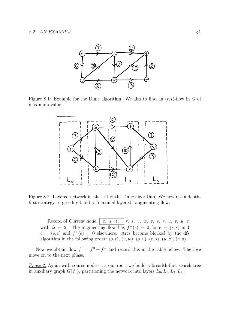
8.2. AN EXAMPLE 81

Figure 8.1: Example for the Dinic algorithm. We aim to find an (r, t)-flow in G ofmaximum value.

Figure 8.2: Layered network in phase 1 of the Dinic algorithm. We now use a depth-first strategy to greedily build a “maximal layered” augmenting flow.

Record of Current node: r, s, t, r, s, v, w, v, s, r, u, v, u, r

with ∆ = 2. The augmenting flow has f+(e) = 2 for e = (r, s) ande = (s, t) and f+(e) = 0 elsewhere. Arcs become blocked by the dfsalgorithm in the following order: (s, t), (v, w), (s, v), (r, s), (u, v), (r, u).

Now we obtain flow f 1 = f 0 + f+ and record this in the table below. Then wemove on to the next phase.

Phase 2: Again with source node r as our root, we build a breadth-first search treein auxiliary graph G(f 1), partitioning the network into layers L0, L1, L2, L3.


Figure 8.3: Layered network in phase 2 of the Dinic algorithm. Our depth-first scanwill only find paths r-s-v-t and r-u-v-t.

Here is our summary of the Flow Augmentation Procedure for this layered net-work.

Record of Current node: r, s, v, t, r, u, v, w, v, t, r, u, r

with ∆ = 5 and then ∆ = 2. The augmenting flow f+ is given by the dataBELOW and arcs become blocked in the following order: (r, s), (v, w),(u, v), (r, u).

As before, we obtain our next flow f 2 = f 1 + f+ and record this in the tablebelow. Then we move on to Phase 3.

Phase 3: From root r, we build a breadth-first search tree in the latest auxiliary graphG(f 2), this time obtaining a layered network of length ` = 4.

We summarize the Flow Augmentation Procedure as follows:

Record of Current node: r, u, s, v, t, r, u, s, u, r with ∆ = 2

(blocking e = (s, v)).

Now we obtain our next flow f 3 = f 2 + f+ and record this in the table. Thenwe move on to Phase 4. But in Phase 4, our Breadth-First Search routine findsthat t is not reachable from r. So the algorithm terminates. The flow f = f 3 is aflow of maximum value and the cut (S; S) with S = r, u, s consisting of the nodesreachable from r in Phase 4 is minimum capacity cut.

8.3. ANALYSIS OF THE DINIC ALGORITHM 83

Figure 8.4: Layered network in phase 3 of the Dinic algorithm. Our depth-first scanwill find only one path: r-u-s-v-t.

8.3 Analysis of the Dinic algorithm

The previous section presented the Dinic algorithm for maximum flow through anetwork. This section contains some of the analysis of this algorithm, but not a fullproof.

Correctness: The proof that the algorithm finds both a max flow and a mincut is the same as for the Ford-Fulkerson algorithm: if there is no (r, t)-path in theauxiliary network G(f), then the partition S, S of vertices into reachable (from r)and unreachable gives a cut in G whose forward capacity is “all used up”. So thecapacity of the cut (S; S) is equal to the value of the current flow from r to t. Asproved earlier in class, this implies that both are optimal.

Limit on Number of Phases: The key difference between Dinic and our earlierapproach is that the choice to stick with the same auxiliary network until the aug-menting flow is maximal (as opposed to discarding this network as soon as a singleaugmenting path is found, as in Ford-Fulkerson) provides us with a strict limit onthe number of phases (or auxiliary networks) that the algorithm must pass through.

Each phase begins with a breadth-first search routine which partitions the auxil-iary network into layers L0, L1, L2, . . .. The vertices in Li are reachable from r by adirected path of length i, but by no shorter path. Our goal is to prove that t moves toa higher layer (i.e., a layer with a larger subscript) in each phase. Once we prove this,we can obtain a good bound on the running time for the Dinic algorithm. Indeed,


each layer is non-empty so there can be at most |V | layers. This proves that therecan be no more than |V | − 1 phases.Claim: If, in the kth phase, we have t ∈ L`k

, then `1 < `2 < `3 < · · · until in somephase t is unreachable from r. In other words, the “length” of the auxiliary networkalways increases.

Proof: Our first step is to prove that the length never decreases. More generally, weprove that no node can be closer to r in the (k + 1)st phase than it was in the kth

phase.Let L0, L1, . . . , L`k

be the partition of the auxiliary network into layers at thebeginning of the kth phase and let L′0, L′1, . . . , L′`k+1

be the partition of the next

auxiliary network into layers at the beginning of the (k + 1)st phase.For each v ∈ V we show that, if Li is the layer containing v in the kth phase and

L′j is the layer containing v in the (k + 1)st phase, then j ≥ i. We prove this byinduction on i.

Certainly the statement holds for i = 0 since L0 = L′0 = r. Now assume it holdsfor all vertices in L0 ∪ L1 ∪ · · · ∪ Li−1 and let v be a vertex in Li. Now suppose thatu0, u1, . . . , uj−1, uj is a directed path in the (k +1)st auxiliary network from u0 = r touj = v. To prove that j ≥ i, we simply consider uj−1. If j were smaller than i, thenuj−1 would belong to L′j−1 and our induction hypothesis would give us j − 1 ≥ i− 1.To be contined . . .

8.4 The Menagerie

Another strange-but-useful variant of network flows goes here.

Exercises

Exercise 8.4.1. Carry out the Dinic Algorithm on the network shown in Figure 8.4.

Exercise 8.4.2. Explain in words the execution of the Dinic Algorithm on a networkwhich is simply a directed path G = (V, A) with V = v0, v1, . . . , vn, A = (vi−1, vi) :1 ≤ i ≤ n arc capacities b(e) = bi for e = (vi−1, vi), source node vr and sink node vt

where we assume t > r.

ZZ


Figure 8.5: Find a maximum flow using the Dinic algorithm.

Nine

The Minimum Cost Flow Problem

Nov. 29, 2010

We now delve into one of the main algorithms of this course. A wide range ofapplied problems can be cast in the language of min-cost flow problems.

9.1 Finding minimum cost flows

We now present an algorithm to find a feasible flow in a network of given value andminimum cost. The next few pages are based on lectures of Jack Edmonds.

Min Cost Flow Problem (mcfp)

Input: Network G = (V, A); a source node r ∈ V ; a sink node t ∈ V ; the demand Dgiven by: Dt = K and Dr = −K; Du = 0 for u ∈ V − r, t; capacities b = b(e) :e ∈ A ≥ 0 on arcs; and costs p = p(e) : e ∈ A ≥ 0 on arcs.

Output: A feasible (r, t)-flow f = (f(e) : e ∈ A) in G of value K such that “totalcost” p · f :=

∑e∈A p(e)f(e) is minimum.

Recall that a feasible flow f satisfies

0 ≤ f ≤ b and ∀ i ∈ V − r, t∑

h(e)=i

f(e)−∑

t(e)=i

f(e) = 0,

where h(e) is the head of arc e and t(e) is the tail. The value of a flow f is equal tothe net amount of flow into the sink t: K =

∑h(e)=t f(e)−

∑t(e)=t f(e).

We now present the “Primal-dual” algorithm using shortest paths (PDSP Al-gorithm, for short) for the MCFP.

86

9.1. FINDING MINIMUM COST FLOWS 87

PDSP Algorithm for MCFP

At stage k of the algorithm, k = 0, 1, 2, ..., we have a feasible flow,

fk = (fk(e) : e ∈ A) of amount Kk

at node t (and of course amount −Kk at node r); And we have a node numberingyk = (yk(u) : u ∈ V ) (the “dual variables”).

We assume by way of induction that fk and yk satisfy Edmonds’ “magic numberconditions” :Magic Number Conditions (MNC)” :

for each e ∈ A, fk(e) < b(e) ⇒ pk(e) ≥ 0, and fk(e) > 0 ⇒ pk(e) ≤ 0,

where pk(e) := p(e)− yk(h(e)) + yk(t(e)).By the Magic Number Theorem to be proved below, the MNC impy that fk is a

cheapest feasible flow (i.e. one that minimizes p · f) of amount Kk at node t.If Kk = K, the amount demanded, stop. Otherwise, as follows, either find an

obstruction to more flow than amount Kk and stop, or else find a feasible fk+1 ofamount Kk+1 > Kk and a node numbering yk+1 satisfying the MNC.

Details of the (k + 1)st iteration

Construct the (k + 1)st auxiliary network G(fk) (as usual, a modification of G deter-mined by the current flow fk):

Gk = (V, Ak), Ak = Ak+ ∪ Ak

−,

where Ak+ = e ∈ A : fk(e) < b(e) and Ak

− = e ∈ A : fk(e) > 0 (i.e., reversearcs).

Recall: For any e ∈ A, e means a “new” arc such that h(e) = t(e) and t(e) = h(e)

and

A= e : e ∈ A.Recall that

pk(e) = p(e)− yk(h(e)) + yk(t(e)) (9.1)

for e ∈ A. Let pk(e) = −pk(e) for e ∈ A. Notice that if we use p(e) = −p(e), we havepk(e) = p(e)− yk(h(e)) + yk(t(e)) which is the same formula as for pk(e). That is, forevery e ∈ A ∪ A, formula (9.1) holds.

Let P k be any shortest (i.e. cheapest) directed path in Gk from r to t relative toarc costs pk = (pk(e) : e ∈ Ak) or if there is no P k then there is an obstruction as in“max flow - min cut”, so stop.

88 CHAPTER 9. THE MINIMUM COST FLOW PROBLEM

For each node u ∈ V , let dk(u) be “the distance of node u from node r, in networkGk relative to pk = (pk(e) : e ∈ Ak)” i.e.

dk(u) = the minimum cost of a directed path in Gk from r to u,or dk(u) = ∞ if there is no directed path in Gk from r to u.

Notice the MNC mean exactly the same as: pk(e) ≥ 0 for each e ∈ Ak. This isimportant because it follows that, to find dk = (dk(u) : u ∈ V ) and some P k, we canuse an algorithm for shortest paths which assumes that pk ≥ 0.

Note. For e ∈ A such that 0 < fk(e) < b(e), we have both e and e in Gk, and we havepk(e) = 0 and pk(e) = 0. This happens often and it helps to make it easier to find dk

and P k. In fact we may get dk(u) = 0, for every u ∈ V , for a sequence of stages k.In this case our algorithm acts exactly like the max flow algorithm.

For each arc e, let

fk+1(e) =

fk(e) + ∆, for e ∈ P k ∩ A;

fk(e)−∆, for e ∈ P k ∩ A;

fk(e), for other e ∈ A.

where ∆ is taken as large as possible such that fk+1 = (fk+1(e) : e ∈ A) satisfies0 ≤ fk+1 ≤ b and such that the value (denoted Kk+1) of fk+1 into node t satisfiesKk+1 ≤ K. That is,

∆ := minb(e)− fk(e) : e ∈ P k ∩ A ∪ fk(e) : e ∈ P k ∩ A ∪ K −Kk.

Note. As in max flow algorithm, fk+1 will satisfy demands of Du = 0 for u ∈ V −r, t,no matter how ∆ is chosen.

Let yk+1 = yk + dk. (i.e. for each u ∈ V , let yk+1(u) = yk(u) + dk(u))Using merely the facts that P k is a shortest directed path from r to t, and that

each dk(u) is the distance from r to u, in Gk relative to (pk(e) : e ∈ Ak), prove that

dk(h(e)) ≤ pk(e) + dk(t(e)) for each e ∈ Ak

and thatdk(h(e)) = pk(e) + dk(t(e)) for each e ∈ P k.

For every e ∈ A∪

A (not only e ∈ Ak), we have

pk+1(e) = p(e)−yk+1(h(e))+yk+1(t(e)) = p(e)−yk(h(e))+yk(t(e))−dk(h(e))+dk(t(e))

Thus pk+1(e) = pk(e) − dk(h(e)) + dk(t(e)). Thus pk+1(e) ≥ 0 for e ∈ Ak andpk+1(e) = 0 for e ∈ P k.

The reader should now consider carefully what the implications are for theseconditions.

9.2. LINEAR PROGRAMMING AND THE MAGIC NUMBER THEOREM 89

9.2 Linear programming and the Magic Number

Theorem

In the previous section, we consider the Primal-Dual Shortest Path (PDSP) algorithmfor finding a minimum cost flow in a network. Here we prove that the algorithm worksby first considering the linear programming formulation of the problem.

Suppose G = (V, A) is a network (directed graph) with source r, sink t, arccapacities (b(e) : e ∈ A) and arc costs (p(e) : e ∈ A), and K ≥ 0 is a target value forour flow.

A feasible flow in G from r to t is a function

f : A → R

satisfying 0 ≤ f(e) ≤ b(e) for all arcs e ∈ A and “flow in = flow out” at each internalnode: ∑

h(e)=v

f(e) =∑

t(e)=v

f(e), (v 6= r, t).

We seek a minimum cost feasible flow f of value K. So this may be formulatedas a linear programming problem

min∑e∈A

p(e)f(e)

subject to∑h(e)=r

f(e)−∑

t(e)=r

f(e) = −K

∑h(e)=v

f(e)−∑

t(e)=v

f(e) = 0 for v 6= r, t

∑h(e)=t

f(e)−∑

t(e)=t

f(e) = K

0 ≤ f(e) ≤ b(e) for e ∈ A

But we find it convenient to eliminate the constraint corresponding to the sourcenode r since it is a linear combination of the other |V | − 1 equality constraints.

With this modification, the dual linear programming problem can be written as

90 CHAPTER 9. THE MINIMUM COST FLOW PROBLEM

follows

max Kz(t)−∑e∈A

b(e)w(e)

subject to

z(u) + w(e) + p(e) ≥ z(v) for all e = (u, v) ∈ A

z(r) = 0

w(e) ≥ 0 for e ∈ A

where we have re-inserted z(r) as a constant to make the expressions uniform1.

9.3 The Menagerie

Exercises


1 Alternatively, we could have left the v = r constraint in the primal and our dual would haveone free variable, which we could then eliminate by setting z(r) = 0 and arriving at the same result.

Bibliography

[1] J.A. Bondy and U.S.R. Murty. Graph Theory with Applications. Elsevier–NorthHolland, New York, 1976.

[2] V. Chvatal. Linear Programming. Freeman, New York, 1983.

[3] S. Even. Graph Algorithms. Computer Science Press, Rockville Maryland, 1979.

[4] M.R. Garey and D.S. Johnson. Computers and Intractability: A Guide to theTheory of NP-Completeness. Freeman, New York, 1979.

[5] C.H. Papadimitriou. Computational Complexity. Addison-Wesley, ReadingMass., 1994.

[6] C.H. Papadimitriou and K. Steiglitz. Combinatorial Optimization: Algorithmsand Complexity. Dover, Mineola, 1998.

[7] M. Sipser. Introduction to the Theory of Computation. PWS Pub. Co., Boston,1997.

[8] R.J. Vanderbei. Linear Programming: Foundations and Extensions (3rd ed.)Springer, New York, 2008.

91

Mincostflow Notes

Documents

Transcript of Mincostflow Notes