Biuletyn WAt Vol. lXi, nr 1, 2012

mimo versus siso — simulation results

Jarosław Michalak, cezary ziółkowski, Bogdan UlJasz

Military University of Technology, Faculty of electronics, 00-908 warsaw, Poland, 2 kaliskiego str.,

jmichalak@wat.edu.pl, cziolkowski@wat.edu.pl, buljasz@wat.edu.pl

Abstract. results of computer simulation tests of the sTBc alamouti MiMo 2 × 2 system in comparison to siso were presented in this paper. The aim was to assess effectiveness of MiMo versus siso in assumed propagation conditions. depending on subscriber motion, propagation conditions as well as antenna system configuration, different results were received. in each configuration, MiMo system was not worse than siso and many times it is significantly better than siso with gain from a few to a dozen or so dB.Keywords: MiMo, alamouti, oFdM, siso, sTBc

1. introduction

among emerging radio technologies with the potential to push the frontiers of wireless capacity, multiple-input-multiple-output (MiMo) system stand out with the promise of many orders of magnitude improvement in spectrum efficiency relative to what is achievable today. Telatar [1] and Foshini [2] were among those who pioneered the concept of MiMo system in the early 1990s. in the mid 1990s, Foshini and his colleagues developed the Bell labs space-time (BlasT) architecture that reports achieving spectral efficiencies in the range of 10-20 b/s/hz for typical configurations. since then, MiMo system has attracted a large amount of research interest.

The idea behind MiMo is that the signals at the Transmitter (Tx antennas) and at the receiver (rx antennas) are combined in such a way that quality of (Ber) or the data rate (bits/s) of communication for each MiMo user is improved. such

224 J. Michalak, C. Ziółkowski, B. Uljasz

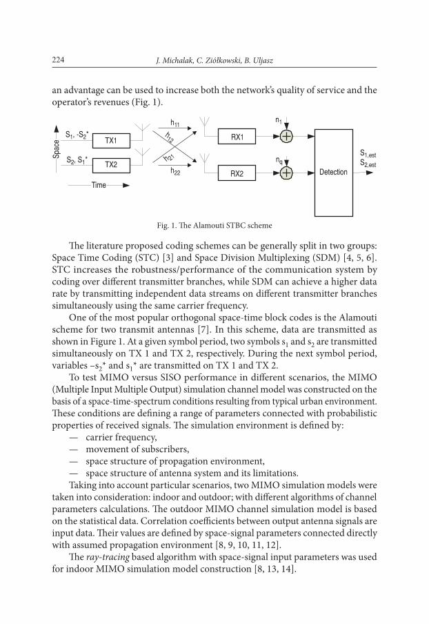
an advantage can be used to increase both the network’s quality of service and the operator’s revenues (Fig. 1).

Fig. 1. The alamouti sTBc scheme

The literature proposed coding schemes can be generally split in two groups: space Time coding (sTc) [3] and space division Multiplexing (sdM) [4, 5, 6]. sTc increases the robustness/performance of the communication system by coding over different transmitter branches, while sdM can achieve a higher data rate by transmitting independent data streams on different transmitter branches simultaneously using the same carrier frequency.

one of the most popular orthogonal space-time block codes is the alamouti scheme for two transmit antennas [7]. in this scheme, data are transmitted as shown in Figure 1. at a given symbol period, two symbols s1 and s2 are transmitted simultaneously on TX 1 and TX 2, respectively. during the next symbol period, variables –s2* and s1* are transmitted on TX 1 and TX 2.

To test MiMo versus siso performance in different scenarios, the MiMo (Multiple input Multiple output) simulation channel model was constructed on the basis of a space-time-spectrum conditions resulting from typical urban environment. These conditions are defining a range of parameters connected with probabilistic properties of received signals. The simulation environment is defined by:

— carrier frequency,— movement of subscribers,— space structure of propagation environment,— space structure of antenna system and its limitations.Taking into account particular scenarios, two MiMo simulation models were

taken into consideration: indoor and outdoor; with different algorithms of channel parameters calculations. The outdoor MiMo channel simulation model is based on the statistical data. correlation coefficients between output antenna signals are input data. Their values are defined by space-signal parameters connected directly with assumed propagation environment [8, 9, 10, 11, 12].

The ray-tracing based algorithm with space-signal input parameters was used for indoor MiMo simulation model construction [8, 13, 14].

225MiMo versus siso — simulation results

diversity of solutions was decisive because of limitations of practical verification abilities in two mentioned above models.

2. simulation environment

2.1. Description of mimo and siso indoor and outdoor channel models

2.1.1. MiMo outdoor channel model

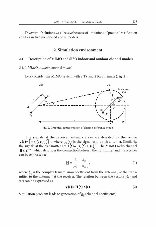
let’s consider the MiMo system with 2 Tx and 2 rx antennas (Fig. 2).

Fig. 2. graphical representation of channel reference model

The signals at the receiver antenna array are denoted by the vector ( ) ( ) ( )1 2, ,

Tt y t y t = y where ( )iy t is the signal at the i-th antenna. similarly,

the signals at the transmitter are ( ) ( ) ( )1 2,T

t s t s t = s . The MiMo radio channel 2 2C ×∈H which describes the connection between the transmitter and the receiver

can be expressed as

11 12

21 22

,h hh h

=

H

(1)

where hij is the complex transmission coefficient from the antenna j at the trans-mitter to the antenna i at the receiver. The relation between the vectors y(t) and s(t) can be expressed as

( ) ( ) ( ).t t t= ⋅y H s

(2)

simulation problem leads to generation of hij (channel coefficients).

226 J. Michalak, C. Ziółkowski, B. Uljasz

Assumptions

it is assumed that all antenna elements in the two arrays have the same polarization and the same radiation pattern. The hij is complex gaussian variable distributed with identical average value. The spatial complex correlation coefficients as elements of the matrix H are given by { }*

ijkl ij klE h ha = . it is independent of transmitter (receiver) number.

Generation of Correlation Channel Coefficients

The correlation channel coefficients hij are generated from zero-mean complex independent of identically distributed random variables ai:

,=A Ca (3)

where [ ] [ ]11 12 21 22 1 2 3 4, , , , , , , TTh h h h a a a a= =A a are 4-dimentional normal vec-tors, C matrix results from the standard cholesky factorization of the correlation matrix

1111 1112 1121 1122

1211 1212 1221 1222

2111 2112 2121 2122

2211 2212 2221 2222

,MIMO

a a a a

a a a a

a a a a

a a a a

=

R

where TMIMO =R CC .

Fig. 3. MiMo channel simulation algorithm

11 12

21 22

=

Hh h

h h

227MiMo versus siso — simulation results

input parameters and simulation assumptions are as follow:sNR — signal to noise ratio of the received signal in dB,c = 3×108 — speed of electromagnetic wave in m/s,fo — carrier frequency in Mhz; in assumption from 1.3 to 1.7 ghz,v — the Ms2 station speed (soldier). in assumption from 1 to 10 [m/s],D — the distance between Ms2 and Ms1 (vehicle) station, in assumption it varies from 50 to 1000 [m],R — local spread radius (see Fig. 2), in assumption, it is from 1 to 100 [m],α — the angle between Ms1 antenna system direction and the line between the centre points of Ms2 and Ms1 antenna systems, in radians,β — the angle between Ms2 antenna system direction and the line between the centre points of Ms2 and Ms1 antenna systems, in radians,γ — the Ms2 station motion direction in relation to the line between the centre points of Ms2 and Ms1 antenna systems, in radians,d/λ — relative distance between particular antennas in Ms2 antenna system, from 0.1 to 4,δ/λ — distance between particular antennas in Ms1 antenna system, from 0.1 to 4,n — the number of the channel state (next simulation point),( )0J ⋅ — Bessel function,

ai — i-th complex variable generated with normal distribution n(0, 1) (i = 1, 2, 3, 4),

OFDMST — oFdM (orthogonal Frequency division Multiplexing) symbol time,

0Dmvf fc

= — maximum value of frequency doppler shift,

1

OFDM

sS

fT

= — frequency of channel parameters changing,

Dmn

s

ff

f= — normalized doppler frequency according to frequency of channel

parameters changing,

arctg RD

∆ = — spread area angle (Fig. 2) (it is possible to assume that

( ) 21.7 17 10 rad−∆ = − ⋅ ).

2.1.2. MiMo indoor channel model

MiMo channel model is the superposition of signals described by eq. (4) induced in particular receiving antennas (Fig. 4):

0 0( )( ) ( ) ( , ) ,i tx t t m t e a += a (4)

228 J. Michalak, C. Ziółkowski, B. Uljasz

where: m(t, a) — modulation function, a — data sequence,

( )

1( ) , ( ( ) )l

Mi t

l l Dl ll

t e t ta a =

= = +∑ — complex function epresenting

an envelope of received signal, M — random number of received rays, l(t) — phase of l-th ray, Dl — doppler shift of pulsation.

equation (4) can be extended to:

0 0( ( ) ( ) )

1 1( ) ( ) ,

mn mnk k

K Mmn i t d t t

kk m

x t t e b a − +Φ +

= =

= ∑ ∑ (5)

where: M — number of Tx antennas, K — number of scattering elements,

2 300 , ( )[MHz]

mnkd t

f

b ll

= = — instant distance between m-th Tx

antenna and n-th rx antenna for k-th scattering element, ( )mn

k tΦ — instant phase of the signal connected with movement of the receiver (doppler effect).

Fig. 4. geometry of simulation indoor MiMo model as well as measuring set. sk — k-th scattering element, v — receiver speed

Figure 5 shows the simulation algorithm for indoor MiMo system.input data were as follow:f0 — system frequency,D — start distance between Tx and rx,s — number of scattering elements,a — Tx antenna angle,v — rx speed,R — spreading area radius.

229MiMo versus siso — simulation results

2.2. Description of the simulation configuration and procedures

2.2.1. simulation models

The configuration shown in Figure 6 was used to assess basic of differences between siso (single input single output) and MiMo techniques using oFdM modulation in assumed channel circumstances.

These tests give the intrinsic performances of each waveform.simulation for different distances was performed between Ms2 and Ms1, as

well as different speed of stations, ideal synchronization, ideal channel estimation and maximum likelihood (Ml) hard detection. The channel type was outdoor. note that the aim is to test the influence of different antenna direction, speed, spreading area and a distance on MiMo efficiency. There is no dwell structure and channel coding implemented. so, the expected values of eb/no are relatively big.

extended model (Fig. 7) was used for additional simulations to have the possibility to assess results for real eb/no values.

random data at the input are coded by alamouti 2×2 sTBc coder. next, oFdM symbols are formed with MPsk mapping. oFdM symbols are transformed (iFFT — inverse Fast Fourier Transform) to time form, and before entering the MiMo (siso) channel(s), cyclic Prefix (cP) is added to each of them. cP is removed at the receiver before transforming the signal to frequency domain. next, the Ml detection and suitable decoding are performed as well as data streams are compared to make a decision about Ber.

Fig. 5. MiMo indoor simulation model algorithm

230 J. Michalak, C. Ziółkowski, B. Uljasz

There were a few simulation options: — subcarriers per oFdM symbol = 512 with 1/32 cP,— oFdM symbol duration — 2 ms,— Modulations: QPsk, 8Psk, 16QaM,— coding: Tc, ldPc,— centre frequency 1.7 ghz with 5 Mhz Bw,— MiMo channel coder type: alamouti 2×2 with Ml detector,— available channel types: siso, MiMo (MiMo1, MiMo2, MiMo3),

awgn,— User speed: 5 km/h, 120 km/h,— distances between users: 50 m, 1000 m.

Fig. 6. oFdM with MiMo test bench 1

Fig. 7. oFdM with MiMo test bench 2

231MiMo versus siso — simulation results

2.2.2. outdoor channel model parameterization

There were 3 types of MiMo channel during simulations (Fig. 8-10; tab. 1-3).Table 1

MiMo1 channel simulation parameters

Parameters Values

R 4 m

a 0 rad

b pi/16 rad

d/l 0.5

d/l 0.5n 0

Table 2MiMo2 channel simulation parameters

Parameters Values

R 4 m

a 0 rad

b pi/16 rad

g pi/2 rad

d/l 0.5

d/l 0.5n 1

Fig. 9. MiMo2 scenario. Ms1 moves. The angle between antenna system direction (Ms1, Ms2) is small

Fig. 8. MiMo1 scenario. no movement. The angle between antenna system direction (Ms1, Ms2) is small

232 J. Michalak, C. Ziółkowski, B. Uljasz

Table 3MiMo3 channel simulation parameters

Parameters Values

R 10 m

a pi/4 rad

b pi/16 rad

g 0

d/l 0.5

d/l 0.5n 1

Fig. 10. MiMo3 scenario. Ms1 moves. almost parallel antenna systems

Remarks to the mentioned above scenarios:1. To have the same (repeatable) simulation conditions, siso channel model

is simply one path from MiMo channel model. amplitude and phase statistics are the same for MiMo as well as for siso case.

2. For extended test bench MiMo3 outdoor channel was used.

2.1.3. indoor channel model parameterization

indoor channel model values of parameters used during simulations can be found in Table 4.

233MiMo versus siso — simulation results

Table 4indoor channel model parameters

Parameters Values

Basic parameters

carrier frequency [Mhz] 1700

Ms2 speed [m/s] 0.5

assumed number of scatters 100

geometric parameters

distance between Tx and rx [m] 27.74

width of the Tx beam [deg] 180

width of the room (corridor) [m] 1.82

Transmitter geometry

number of Ms1 antennas 2

distance between Tx antenna elements [m]8

9

0.5 3 101.7 10⋅ ⋅⋅

angle between direction of the radiation and the transmitter antennas axis [deg] into direction of the radiation 0

Mobile geometry

number of Ms2 antennas 2

distance between rx antenna elements [m] delta_rx = 0.5*lambdac

3. simulation Results

3.1. Results from test bench 1

next figures show examples of simulations’ results as Ber or Per characteristics in a function of Eb/N0 for various simulation scenarios.

Figure 11a shows the Ber characteristic for 50 m distance and 5 kmph user velocity. depending on antenna systems directions (see MiMo1, MiMo2 and MiMo3 description), you can notice some differences in MiMo system efficiency. For larger spread area (10 m for MiMo3 and 4 m for MiMo1), the system operates better.

For moderate speed (5 kmph), the Ber is better than in no movement (about 5 dB at Ber = 10–3) it can be justified by diversity of transmission properties of signal paths. The mean gain MiMo over siso at Ber = 10–3 is about 20 dB.

Figure 11b shows the Ber characteristic for 50 m distance and 120 kmph user velocity. The difference in gain between siso and MiMo is the same in 120 kmph example (unnoticeable differences).

234 J. Michalak, C. Ziółkowski, B. Uljasz

Figure 11c shows the Ber characteristic for 1000 m distance and 5 kmph user velocity. For a distance equal to 1000 m, as in example a) depending on antenna systems directions (see MiMo1, MiMo2 and MiMo3 description) you can notice some differences in MiMo system efficiency. an interesting point is that the best performances are for antenna systems directions near to parallel (MiMo3).

The mean gain MiMo over siso at Ber = 10–2 is about 12 dB. differences in performances of MiMo at Ber = 10–3 are about 10 dB. if a distance between Ms2 and Ms1 is changed to 1000 m (from 50 m as in example a) we have loss of about 13 dB (Ber = 10–4).

Figure 11d shows the Ber characteristic for 1000 m distance and 120 kmph user velocity. as in example b), if a distance between Ms2 and Ms1 is changed to 1000 m we have loss which in 120 kmph is about 13 dB at Ber = 10–3. remember that spread area for MiMo3 is assumed as 10 m while for MiMo2 it is 4 m.

each example shows that the gain of MiMo3 over MiMo2 is about 4 dB.as you can see in Figure 12, for MiMo1 (no movement) dependence of MiMo

system efficiency on antenna system directions is rather small, except of situation

Fig. 11. MiMo in comparison to siso for 4Psk — different distances and Ms2 speed

235MiMo versus siso — simulation results

with parallel antenna location. with this special location, we get gain of about 5 dB at Ber = 10–3.

as you can see in Figure 13, for MiMo2 (speed v = 120 kmph) dependence of MiMo system efficiency on antenna system directions is small and can be neglected. it can be justified by diversity of transmission properties of signal paths. This phenomenon improves Ber to the value as for parallel antenna systems location (see Fig. 12).

Fig. 12. MiMo1 for different direction of antenna systems

Fig. 13. MiMo2 for different direction of antenna systems and v = 120 kmph

Figure 14 shows an influence of spread radius value on the efficiency of MiMo2 variant. as it can be noticed at previous experiments, in Figure 14, you can see that if spread radius is rising, the level of diversity of transmission properties of signal

236 J. Michalak, C. Ziółkowski, B. Uljasz

paths is rising too, leading to decrease in a correlation level between parameters of the channel transmittance matrix hij.

differences in performances of MiMo2 with different spread radius at Ber = 10–3 are about 10 dB.

results from test bench 2

Fig. 15. MiMo versus siso Ber and Fer characteristics with perfect synchronization, 2-ms slot duration, Turbo code Fec with code rate ½, 2 bits/symbol, 5 Mhz bandwidth, no spreading,

no jamming, no time shift, no frequency shift, MiMo3

Fig. 14. MiMo2 with different spread radius

237MiMo versus siso — simulation results

depending on configuration parameters of channel, especially indoor case, the different results can be observed (with fluctuations of a couple of dB).

gain of MiMo against siso at Ber = 10–3 is about 10 dB.

Fig. 16. MiMo versus siso Ber and Fer characteristics with perfect synchronization, 2-ms slot duration, Turbo code Fec with code rate ½, 2,3,4 bits/symbol, 5 Mhz bandwidth, no spreading, no

jamming, no time shift, no frequency shift, MiMo3

4. Conclusions

summing up all simulations concerning alamouti 2×2 sTBc MiMo system, we can write the following summarized conclusions:

— application of MiMo system in awgn channel (practically channel with low dispersion) does not introduce such gain as with high dispersion channel but does not worsen efficiency of the link.

— Potential mean Ber improvement in MiMo over siso in outdoor as well as indoor channel can be about 10 dB on average, at Ber = 10–3. it de-pends on modulation type, distance, antenna system direction, movement, spreading area and maybe others, not examined here parameters. notice that with no movement, parallel antenna system location has much better performance than others (about 5 dB difference).

— if spread radius is too small (narrow tunnel, corridor etc.), the gain of MiMo can be smaller in comparison to others by a value up to 5 dB because of bad correlation properties between transmission paths.

238 J. Michalak, C. Ziółkowski, B. Uljasz

— we have no answer concerning behaviour of MiMo system with directional antennas (which can be used in practice e.g. as an element of uniform), but we expect that the gain over siso can be smaller.

Received January 12 2011, revised February 2011.

reFerences

[1] e. Telatar, Capacity of multiantenna Gaussian channels, aT&T Bell laboratories, Tech. Memo., June 1995.

[2] g.J. Foshini, Layered space-time architecture for wireless communication in a fading environment when using multielement antennas, Bell labs. Tech. J., autumn 1996.

[3] V. Tarokh, n. seshadri, a.r. calderbank, space-time codes for high data rate wireless com-munication: performance criterion and code construction, ieee Transactions on information Theory, 44, 3, March 1998, 744-756.

[4] g.J. Foschini, M.J. gans, on limits of wireless communications in a fading environment when using multiple antennas, aT&T Bell labs internal Tech. Memo, sept. 1995. Published in wireless Personal communications, 6, 3, March 1998, 311-335.

[5] g.g. raleigh, J.M. cioffi, spatio-temporal coding for wireless communication, ieee Trans. on communications, 46, 3, March 1998, 357-366.

[6] a. van zelst, space division multiplexing algorithms, in Proc. of the 10th Mediterranean elec-trotechnical conference (Melecon) 2000, 3, May 2000, 1218-1221.

[7] s.M. alamouti, A simple transmit diversity technique for wireless communications, ieee Journal on selected areas in communications, 16, 8, oct. 1998, 1451-1458. decoding (equalisation) methods.

[8] F.P. Fontan, P.M. espineira, Modelling the Wireless Propagation Channel. A simulation Approach with MATLAB, J. wiley & sons, chichester, 2008.

[9] J.P. kermoal, l. schumacher, k.i. Pedersen, P.e. Mogensen, F. Frederiksen, A stochastic MiMo Radio Channel Model with Experimental Validation, ieee Journal on selected areas in communications, 20, 6, august 2002.

[10] a. abdi, M. kaveh, A space-Time Correlation Model for Multielement Antenna systems in Mobile Fading Channel, ieee Journal on selected areas in communications, 20, 3, april 2002.

[11] P-y. chen, h-J. li, Modelling and Application of space-Time Correlation for MiMo Fading signals, ieee Transaction on Vehicular Technology, 56, 4, July 2007.

[12] k.e. Baddour, n. Beaulieu, Accurate simulation of Multiple Ceoss-Correlated Rician Fading Channel, ieee Transaction on communications, 52, 11, november 2004.

[13] a.a.M. saleh, r.a. Valenzuela, statistical Model for indoor Multipath Propagation, ieee Journal on selected areas in communications, 5, 2, 1987.

[14] F. Perez Fontan, P. Marino espineira, Modelling the Wireless Propagation Channel — A simu-lation Approach with MATLAB, wiley 2008.

239MiMo versus siso — simulation results

J. Michalak, c. ziółkowski, B. UlJasz

Efektywność systemu mimo względem siso — wyniki badań symulacyjnychstreszczenie. w artykule zaprezentowano wyniki symulacji komputerowej systemu wieloantenowego MiMo 2×2 (ang. Multiple input Multiple output) z koderem sTBc (ang. space Time Block Coding) alamoutiego w porównaniu do systemu siso (ang. single input single output). celem badania było określenie stopnia efektywności układu MiMo zależnie od prędkości i kierunku ruchu korespondenta, warunków propagacji oraz konfiguracji anten. zależnie od założeń symulacyjnych uzyskano wyniki potwierdzające przewagę MiMo nad siso w zakresie od kilku do kilkunastu dB.słowa kluczowe: MiMo, alamouti, oFdM, siso, sTBc