MIMO System Technology for Wireless Communications

29

2Theory and Practice of MIMO Wireless Communication Systems

Dimitra Zarbouti, George Tsoulos, and Dimitra Kaklamani

CONTENTS

Summary ................................................................................................................302.1 Shannon’s Capacity Formula.....................................................................302.2 Extended Capacity Formula for MIMO Channels.................................31

2.2.1 General Capacity Formula.............................................................312.2.2 Transformation of the MIMO Channel into n

SISO Subchannels......................................................................................32

2.2.3 No CSI at the Transmitter..............................................................342.2.4 CSI at the Transmitter.....................................................................352.2.5 Channel Estimation at the Transmitter........................................35

2.3 Remarks on the Extended Shannon Capacity Formula ........................362.3.1 Bounds on MIMO Capacity ..........................................................362.3.2 Capacity of Orthogonal Channels ................................................382.3.3 Effective Degrees of Freedom .......................................................38

2.4 Capacity of SIMO — MISO Channels......................................................392.5 Stochastic Channels .....................................................................................40

2.5.1 Ergodic Capacity .............................................................................402.5.2 Outage Capacity ..............................................................................41

2.6 MIMO Capacity with Rice and Rayleigh Channels ..............................412.6.1 MIMO Channel Matrix for Rayleigh Propagation

Conditions ........................................................................................422.6.2 MIMO Channel Matrix for Ricean Propagation Conditions ...432.6.3 Channel Matrix with Spatial Fading Correlation ......................45

2.7 Simulations ...................................................................................................472.7.1 MIMO Capacity for a Rayleigh Channel without Spatial

Fading Correlation ..........................................................................482.7.2 MIMO Capacity for a Rayleigh Channel with Spatial

Fading Correlation ..........................................................................492.7.3 MIMO Capacity for a Ricean Channel ........................................50

4190_book.fm Page 29 Tuesday, February 21, 2006 9:14 AM

30 MIMO System Technology for Wireless Communications

Appendix 2A .........................................................................................................51Appendix 2B ..........................................................................................................52Appendix 2C..........................................................................................................53References...............................................................................................................54

Summary

This chapter introduces the principles of MIMO systems employing thenecessary mathematical analysis to consider the achieved capacity perfor-mance. In this context, flat fading across time and frequency is considered,and the Rayleigh model is employed for describing the wireless channel.Furthermore, the case of spatial selective fading is examined by consideringLOS propagation, with the Ricean model.

The mathematical representation of the MIMO system is performedthrough a complex matrix, which depends on the scenario considered eachtime (i.e., flat or selective spatial fading). The capacity achieved by the MIMOchannel in all the above cases is studied with the use of the Shannon extendedcapacity formula. The capacity performance results, developed from thesimulations performed, are related to the number of the multiple antennaelements that the Rx and the Tx are equipped with, the distance betweenthem and the degree of correlation evidenced.

2.1 Shannon’s Capacity Formula

Shannon’s capacity formula approximated theoretically the maximumachievable transmission rate for a given channel with bandwidth B, trans-mitted signal power P and single side noise spectrum N

o

, based on theassumption that the channel is white Gaussian (i.e., fading and interferenceeffects are not considered explicitly).

(2.1)

In practice, this is considered to be a SISO scenario (single input, singleoutput) and Equation 2.1 gives an upper limit for the achieved error-freeSISO transmission rate. If the transmission rate is less than C

bits/sec (bps),then an appropriate coding scheme exists that could lead to reliable anderror-free transmission. On the contrary, if the transmission rate is more thanC

bps, then the received signal, regardless of the robustness of the employedcode, will involve bit errors.

C BP

N Bo

= +log2 1


Theory and Practice of MIMO Wireless Communication Systems

31

2.2 Extended Capacity Formula for MIMO Channels

For the case of multiple antennas at both the receiver and the transmitterends (Figure 2.1), the channel exhibits multiple inputs and multiple outputsand its capacity can be estimated by the extended Shannon’s capacity for-mula, as described below.

2.2.1 General Capacity Formula

We consider an antenna array with nt

elements at the transmitter and anantenna array with nr

elements at the receiver. The impulse response of thechannel between the j

th transmitter element and the i

th receiver element isdenoted as hi,j

(

,t

). The MIMO channel can then be described by the nr

×

nt

H

(

,t

) matrix:

(2.2)

The matrix elements are complex numbers that correspond to the attenu-ation and phase shift that the wireless channel introduces to the signalreaching the receiver with delay

. The input-output notation of the MIMOsystem can now be expressed by the following equation:

(2.3)

where denotes convolution, s

(t

) is a nt

×

1 vector corresponding to the nt

transmitted signals, y

(t

) is a nr

×

1 vector corresponding to the nr

receivedsignals and u

(t

) is the additive white noise.

FIGURE 2.1

The MIMO channel.

Channel H

Tx

nt nr

Rx

H( , )

( , ) ( , ) ( , )

( ,, , ,

,t

h t h t h t

hnt

=

1 1 1 2 1

2 1

�

tt h t h t

h t h

n

n n

t

r r

) ( , ) ( , )

( , ) (

, ,

, ,

2 2 2

1 2

�

� � � �, ) ( , ),t h tM nR t

�

y H s u( ) ( , ) ( ) ( )t t t t= +

4190_book.fm 1 Tuesday, February 21, 2006 9:14 AM


If we assume that the transmitted signal bandwidth is narrow enough thatthe channel response can be treated as flat across frequency, then the discrete-time description corresponding to Equation 2.3 is

(2.4)

The capacity of a MIMO channel was proved in [1, 4] that can be estimatedby the following equation:

(2.5)

where H

is the nr

×

nt

channel matrix, is the covariance matrix of thetransmitted vector s, HH

is the transpose conjugate of the H

matrix and p

isthe maximum normalized transmit power. Equation 2.5 is the result ofextended theoretical calculations, and its practical use is not obvious. Never-theless, we can perform linear transformations at both the transmitter andreceiver converting the MIMO channel to SISO subchannels(given that the channel is linear) and, hence, reach more insightful results.These transformations can be found in [1] and are briefly described in thefollowing section.

2.2.2 Transformation of the MIMO Channel into n SISO Subchannels

Every matrix can be decomposed accordingly to its singular val-ues. Suppose that for the aforementioned channel matrix this transformationis given by Equation 2.6.

(2.6)

where the matrices U

, V

are unitaries of dimensions nr

×

nr

and nt

×

nt

accordingly, while D

is a non-negative diagonal matrix of dimensions nr

×

nt

.The diagonal elements of matrix D

are the singular values of the channelmatrix H

. The algorithm of singular value decomposition that provides theabove transformation can be found in [2].

The operations that lead to the linear transformation of the channel inton

= min(nr

, nt

) SISO subchannels are described as follows: First, the trans-mitter multiplies the signal to be transmitted x

with the matrix V

, the receivermultiplies the received signal r

and noise with the conjugate transpose ofthe matrix U

. The above are presented in Equation 2.7 through Equation 2.9.

(2.7)

r Hs u= +

Ctr p

ssH

ss

= +( )max log det( )R

I HR H2

Rss

n n nr t= min( , )

H ×�n nr t

H UDV= H

s V x=


Theory and Practice of MIMO Wireless Communication Systems

33

(2.8)

(2.9)

Substituting Equation 2.4 into Equation 2.8 gives:

Since U

and V

are unitary matrices, they satisfy , andhence:

(2.10)

Each component of the received vector y

can be written as:

(2.11)

where k

are the singular values of matrix H

according to the transformationthat took place above. Equation 2.11 implies that the initial (nr

, nt

) MIMOsystem has been transformed into n

= min(nr

, nt

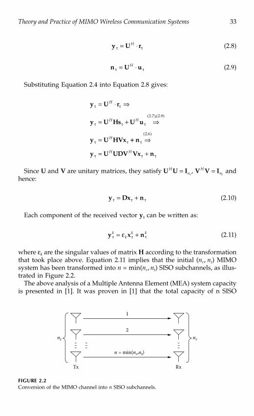
) SISO subchannels, as illus-trated in Figure 2.2.

The above analysis of a Multiple Antenna Element (MEA) system capacityis presented in [1]. It was proven in [1] that the total capacity of n SISO

FIGURE 2.2

Conversion of the MIMO channel into n

SISO subchannels.

y U r= H

n U u= H

y U r

y U Hs U u

y U HVx

=

= +

=

H

H H

H

( . ),( . )2 7 2 9

++

= +

n

y U UDV Vx n

( . )2 6

H H

U U IHnr

= V V IHnt

=

y Dx n= +

y x nkk

k k= +

Tx

1

2

n = min(nr,nt)

nt

Rx

nr



subchannels is the sum of the individual capacities and as a result the totalMIMO capacity is:

(2.12)

where pk is the power allocated to the kth subchannel and is its powergain. We notice that according to the singular value decomposition algorithm

2k, k = 1, 2, …, n are the eigenvalues of the HHH matrix, which are always

non-negative. Furthermore, regardless of the power allocation algorithmused, pk must satisfy

because of the wanted power constraint.At this point, there are two cases of particular interest that need further

consideration: the knowledge (or not) by the transmitter of the Channel StateInformation (CSI). These are described in the following sections.

2.2.3 No CSI at the Transmitter

Considering Equation 2.12, we notice that the achieved capacity depends onthe algorithm used for allocating power to each subchannel. The theoreticalanalysis assumes the channel state known at the receiver. This assumptionstands correct since the receiver usually performs tracking methods in orderto obtain CSI, however the same consideration does not apply to the transmitter.

When the channel is not known at the transmitter, the transmitting signals is chosen to be statistically non-preferential, which implies that the nt

components of the transmitted signal are independent and equi-powered atthe transmit antennas. Hence, the power allocated to each of the nt subchan-nels is pk = p/nt. Applying the last expression to Equation 2.5 gives:

(2.13)

or

(2.14)

Equation 2.14 can be produced from Equation 2.13 as described in greaterdetail in Appendix 2A.

C pk k

k

n

= +( )=

log22

1

1

k2

p pk

k

n

=1

Cpnt

H= +log det2 I HH

Cpnt

k

k

n

= +=

log22

1

1


Theory and Practice of MIMO Wireless Communication Systems 35

2.2.4 CSI at the Transmitter

In cases in which the transmitter has knowledge of the channel, it canperform optimum combining methods during the power allocation process.In that way, the SISO subchannel that contributes to the information transferthe most is supplied with more power.

One method to calculate the optimum power allocation to the n subchan-nels is to employ the waterpouring algorithm (a detailed discussion of thisalgorithm can be found in [3]).

Considering the assumption of CSI at the transmitter, we can proceed tothe following capacity formula.

(2.15)

The difference between Equation 2.14 and Equation 2.15 is the coefficientk that corresponds to the amount of power that is assigned to the kth

subchannel. This coefficient is given by:

(2.16)

and satisfies the constraint

.

The goal with the waterpouring algorithm is to find the optimum k thatmaximizes the capacity given in Equation 2.15.

2.2.5 Channel Estimation at the Transmitter

As mentioned earlier, the CSI is not usually available at the transmitter. Inorder for the transmitter to obtain the CSI, two basic methods are used: thefirst is based on feedback and the second on the reciprocity principle.

In the first method the forward channel is calculated by the receiver andinformation is sent back to the transmitter through the reverse channel. Thismethod does not function properly if the channel is changing fast. In thatcase, in order for the transmitter to get the right CSI, more frequent estima-tion and feedback are needed. As a result, the overhead for the reversechannel becomes prohibitive. According to the reciprocity principle, theforward and reverse channels are identical when the time, frequency andantenna locations are the same. Based on this principle the transmitter mayuse the CSI obtained by the reverse link for the forward link. The main

Cp

nk

tk

k

n

= +=

log22

1

1

k kE s= { }2

kk

n

tn=

=1



problem with this method emerges when frequency duplex schemes areemployed.

2.3 Remarks on the Extended Shannon Capacity Formula

In this section we will use mathematical tools in order to derive the theoreticalupper and lower bounds of MIMO capacity. The algebraic expressions used,as well as the assumptions considered here, are summarized in Section 2.3.1.

In Section 2.3.3 we introduce the Effective Degrees of Freedom (EDoF),which we will use for the simulation justification in Section 2.7.

2.3.1 Bounds on MIMO Capacity

The lower and upper bounds of MIMO capacity were first derived in [1].We proceed with a short description of those bounds. Four basic assumptionsare considered in the following, summarized here for simplicity.

• The transmitter has no previous knowledge of the channel.• The parallel subchannels produced by the decomposition of the

MIMO channel are independent.• The wireless channel is submitted to Rayleigh fading.• The transmitter antenna array elements are less than the receiver’s

antenna elements (nt < nr).

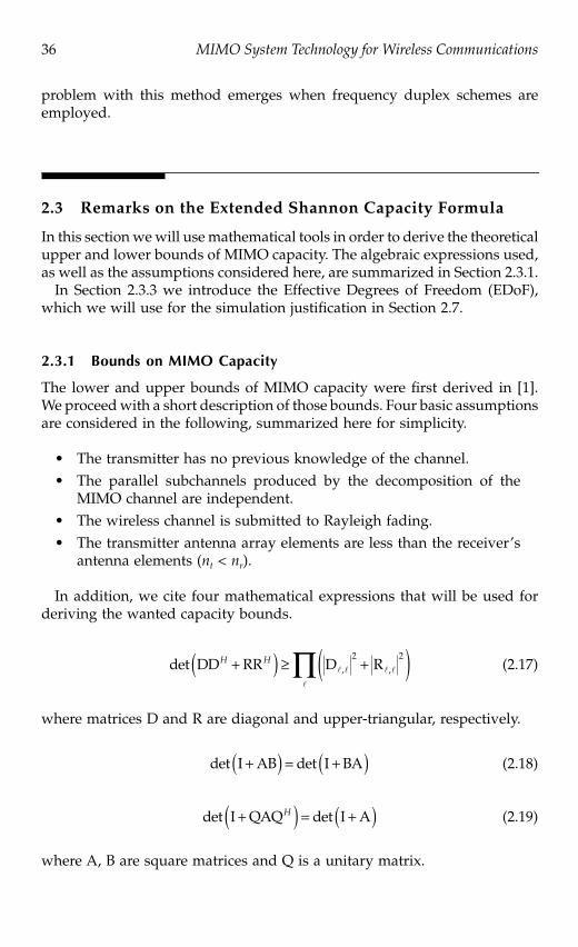
In addition, we cite four mathematical expressions that will be used forderiving the wanted capacity bounds.

(2.17)

where matrices D and R are diagonal and upper-triangular, respectively.

(2.18)

(2.19)

where A, B are square matrices and Q is a unitary matrix.

det , ,DD RR D RH H+( ) +( )� � � �

�

2 2

det detI AB I BA+( ) = +( )

det detI QAQ I A+( ) = +( )H



(2.20)

where X is a non-negative definite matrix.Since the channel is submitted to Rayleigh fading, the channel matrix H

is given by HW, which is referred to as spatially white matrix. The elementsof HW can be modeled as zero mean circularly symmetric complex Gaussian(ZMCSCG) random variables. The HW has particular statistical propertiesthat can be found in [3, 12].

We consider the transformation HW = QR, where Q is a unitary and R isan upper-triangular matrix. This tranformation is referred to as HouseholderTransformation [5]. According to this transformation the elements of R abovethe main diagonal are statistically independent, while the magnitude of themain diagonal entries are chi-squared distributed with 2nr , 2(nr – 2 + 1), …,2(nr – nt + 1) degrees of freedom.

Using Equation 2.13:

(2.21)

Equation 2.21 corresponds to the lower capacity bound and practicallyshows that this bound is defined by the sum of the capacities of nt indepen-dent subchannels with power gains that follow the chi-square distributionwith 2nr, 2nr – 2, …, 2(nr – nt + 1) degrees of freedom.

In order to find the upper bound of the capacity, Equation 2.13 is usedagain:

(2.22)

The upper bound of the capacity is the sum of the capacities of nt inde-pendent subchannels, with power gains chi-squared distributed and withdegrees of freedom 2(nr + nt – 1), 2(nr + nt – 3), …, 2(nr – nt + 1). The differenceof the mean values of the upper and lower bounds is less than 1b/s/Hz.

det ,X X( ) � �

�

Cpn

pnt

H

t

= + = +log det log det2 2I HH I QRRR Q

I RR

H H

t

HCpn

= +

( . )

log det

2 19

2 +( . )

,log2 17

2

21

pn

Rt

� �

�

Cpn

Rt

nt

+=

log ,2

2

1

1 � �

�

Cpn

R Rt

m

m

nt

+ += +

log , ,2

2 2

1

1 � � �

�=� 1

nt



2.3.2 Capacity of Orthogonal Channels

It is interesting to study the case where the capacity of the MIMO channelis maximized. We consider the simple case of nr = nt = n, along with a fixedtotal power transfer through the SISO subchannels (i.e., , where ais a constant). The capacity in Equation 2.14 is concave in the variables 2

k (k= 1, 2, …, n) and, as a result, it is maximized when 2

k = 2i = a/n, (k, i = 1, 2,

…, n). The last equation reveals that the HHH matrix has n equal eigenvalues.Hence, H must be an orthogoal matrix, i.e., . Substitut-ing into Equation 2.13:

(2.23)

If , the matrix H satisfies , hence, Equation 2.13 becomes:

(2.24)

The last equation indicates that the capacity of an orthogonal MIMO channelis n times the capacity of the SISO channel.

2.3.3 Effective Degrees of Freedom

Based on Equation 2.14, we can assume that in high SNR regime, capacitycan increase linearly with n. Specifically, for high SNR regimeEquation 2.14 becomes:

(2.25)

However, this assumption is not always confirmed. For some subchannelsis much smaller than one, and as a result the information transferred

by these channels is nearly zero. This phenomenon is present in at least threecases:

• when the transmission is serviced through a low-powered device• when there is a long-range communication application• when there is strong fading correlation between subchannels

In the last case, the fading induced to a certain subchannel may cause theminimization of its corresponding 2

k .

= =kn

k a12

HH H H IH Hna n= = ( )/

HH IHna n= ( )/

Cpan

C npan

n= + = +log det log2 2 2 1I I22

H i j,

21= HH IH

nn=

Cpn

n C n pn= + = +( )log det log2 2 1I I

( )kp n2 1/ �

Cpn k

k

n

=

log22

1

( )kp n2 /



In practice, the aforementioned cases are very likely to happen, therefore,the concept of EDoF is introduced. Intuitively, the EDoF value correspondsto the number of subchannels that actually contribute to the informationtransfer. In a more mathematical approach, the EDoF value indicates thenon-zero singular values of the channel matrix H. A more detailed descrip-tion of the EDoF can be found in [1].

2.4 Capacity of SIMO — MISO Channels

Single input, multiple output (SIMO) and multiple input, single output(MISO) channels are special cases of MIMO channels. In this paragraph wediscuss the capacity formulas for the case of SIMO and MISO channels.

For a SIMO channel nt = 1, so ; hence, the CSI at thetransmitter does not affect the SIMO channel capacity:

(2.26)

If we consider then (the proof can be found in Appendix 2B).Hence Equation 2.26 becomes:

(2.27)

For a MISO channel nr = 1 and . With no CSI at thetransmitter, the capacity formula can be expressed as:

(2.28)

If we make the same assumption as earlier and consider that then (the proof is cited in Appendix 2B); hence, Equation 2.28 becomes:

(2.29)

Comparing Equation 2.29 and Equation 2.27 we can see that CSIMO > CMISO.This is because the transmitter, as opposed to the receiver, cannot exploitthe antenna array gain since it has no CSI and, as a result, cannot retrieve thereceiver’s direction.

n n nr t= =min( , ) 1

C pSIMO = +( )log2 121

hi

21= 1

2 = nr

C p nSIMO r= +( )log2 1

n n nr t= =min( , ) 1

CpnMISO

t

= +log2 121

hi

21=

12 = nt

C pMISO = +( )log2 1



2.5 Stochastic Channels

In order to use the aforementioned capacity formulas, it is necessary to obtainthe channel matrix expression. There are many spatial channel models thatare used for this purpose ([6–11]).

The simulations that take place in Section 2.7 consider a stochastic channelapproach. Specifically, the Rayleigh and the Rice models are used. Thedescription of these models is cited below. Consequently, under the stochas-tic channel consideration, the capacity achieved becomes a random variable,and in order to study its behavior, we use stochastic quantities, as describedbelow.

2.5.1 Ergodic Capacity

The ergodic capacity of a MIMO channel is the ensemble average of theinformation rate over the distribution of the elements of the channel matrixH [3], and it is given by:

(2.30)

When there is no CSI at the transmitter, we can substitute Equation 2.13into Equation 2.30, so the ergodic capacity is given by

(2.31)

Whereas with CSI at the transmitter we use Equation 2.15, and the ergodiccapacity is given by:

(2.32)

Figure 2.3 illustrates the ergodic capacity for different antenna configurationsas a function of the SNR, when the channel is unknown at the transmitter.As expected, the ergodic capacity increases with SNR. In addition, theergodic capacity of a SIMO channel appears to be greater than the ergodiccapacity of a MISO channel. The reason for this behavior, as previouslyexplained, lies in the fact that the transmitter cannot exploit the antennaarray gain since it has no CSI.

C E I= { }

C Epnt

H= +log det2 I HH

C Epnt

k k

k

n

= +=

log22

1

I



2.5.2 Outage Capacity

The outage capacity quantifies the level of capacity performance guaranteedwith a certain level of reliability [3, 12]. For q% outage capacity Cout,q, indicatesthe maximum capacity level the system can achieve with probability(100 – q)%. For stochastic channels we can observe that there is always apossibility of outage for a given MIMO system realization, regardless of thewanted rate. Hence, there is a tradeoff between the system’s outage capacityand the achieved information rate.

2.6 MIMO Capacity with Rice and Rayleigh Channels

In this section we discuss the capacity expressions for the cases of Rayleighand Ricean channels, as well as when spatial fading correlation is inducedto the signal due to the limited distance between the array elements (the trans-mitter is considered blind for the discussion below, i.e., does not have CSI).

When the wireless environment is characterized by strong multipath activ-ity, then the number of paths between the transmitter and receiver allowsthe use of the central limit theorem [13] and the envelope of the receivedsignal follows the Rayleigh distribution. However, in cases that the location

FIGURE 2.3Ergodic capacity as a function of SNR and number of elements.

50

45

40

35

30

25

20

15

Ergo

dic

capa

city

10

5

05 10 15

SNR(dB)20 25

(4, 4)

Rayleigh channel, ergobic capacity as function of SNR

(2, 2)

(1, 4) (2, 4)

(4, 4)

(1, 1)



of buildings leads to the street waveguide propagation phenomenon, andin areas near the base station where a line of sight (LOS) component maydominate, the Ricean distribution is more suitable. The receiver in that sce-nario “sees” a dominant signal component along with lower power compo-nents caused by multipath. The dominant component that reaches thereceiver may not be the result of LOS propagation, e.g., the dominant com-ponent may be the mean value of strong multipaths caused by large scatter-ers. The Ricean K-factor of the channel is defined as the ratio of the powersof the dominant and the fading components [13].

(2.33)

Obviously, K = 0 indicates a Rayleigh fading channel while K indicatesa non-fading one.

2.6.1 MIMO Channel Matrix for Rayleigh Propagation Conditions

The channel matrix H in Equation 2.31 depends on the channel model.Specifically, in cases where the wireless channel is submitted to Rayleighfading and the array antennas do not introduce additional correlation to thetransmitted/received signal, the channel matrix becomes spatially white.

The ergodic capacity formula under the assumption of Rayleigh channelsand equal power allocation is (following the analysis in Section 2.5.1):

(2.34)

Equation 2.34 is used for the simulations concerning the Rayleigh channelthat will be shown in the next section.

Under the assumption of , it would be interesting to study thecase of n [3]. Using the strong law of large numbers [14] we get:

(2.35)

Therefore, the Rayleigh channel capacity bound is given by:

when n (2.36)

KA=

2

22

C Epnt

H= +log det2 I H HW W

n n nr t= =

1n

as nHnH H IW W( )

C p p nn

n n

n+( ) = +( ) =log det log2 2 1I I +( )log2 1 p

C n p+( )log2 1



Considering the last expression, two things can be noticed:

• Capacity does not depend on the nature of the channel matrix, as itincreases linearly with n for a fixed SNR.

• Every 3 dB increase of SNR corresponds to an n bits/sec/Hz increasein capacity.

2.6.2 MIMO Channel Matrix for Ricean Propagation Conditions

In the presence of a dominant component between the transmitter and thereceiver, the wireless channel can be modeled as the sum of a constant anda variable component caused by scattering [3, 15].

(2.37)

In Equation 2.37 HRice is the MIMO channel matrix, HRayleigh is the MIMOmatrix corresponding to the variable component, HLOS is the MIMO matrixcorresponding to the constant signal component, K is the Ricean–K factorand 0 is the phase shift of the signal when propagating from a transmittingantenna element to the corresponding receiving antenna element.

The HRayleigh matrix is spatially white, and its structure was describedearlier in this chapter. HLOS can be derived by the procedure described inthe following (for more details see [15]).

The general configuration of a multiple transmitting and receiving antennaarray is illustrated in Figure 2.4.

In Figure 2.4, R is the distance between the transmitter and the receiverand d is the interelement distance. The matrix HLOS is given by:

(2.38)

FIGURE 2.4Geometry of a Tx and an Rx linear antenna array.

Tx Rx R

R’

d d

H H HRice LOS Rayleigh=+

++

KK

eK

j

11

10

HLOS =

11

1

1

e e

e

e

e e

j j n

j

j

j n

t

r

��

� � �

( )

( ) j nr( )2 1�



where is the angle corresponding to phase shift between the neighbor arrayelements.

In order to simplify the analysis, the distance between the receiving andthe transmitting antennas is assumed substantially larger than the distancebetween the antenna elements. So, under the assumption of , isminimized to the point that it can be omitted from the matrix in Equation2.38 (see Appendix 2C for the proof). In that case HLOS is given by an nr × nt

matrix, with ones as elements (we refer to this matrix as H(1)).Also, it is obvious that 0 affects the contribution of HLOS to HRice. For reasons

of simplicity it is assumed that

0 = /4, so ej 0 =

As a result, the real and the imaginary parts of the HRice elements are influ-enced in the same manner. After some manipulation, Equation 2.37 becomes:

(2.39)

Equation 2.39 is used to produce the simulation results shown in the nextsection.

The assumptions made regarding the Ricean channel analysis can be sum-marized as follows:

• The dominant component is considered to be caused by LOS prop-agation.

• The distance between the transmitter and the receiver is consideredsubstantially larger than the interelement distance.

Although these assumptions might not always be valid, the results indicatethe effect of the dominant component on the MIMO system capacity, gener-ally. In cases that the dominant signal component is caused by directionalmultipath propagation, this component is time varying, and hence, the aboveanalysis cannot be applied.

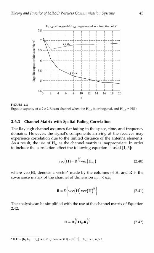
However, the case can be found in multibase operations [3]. In thesescenarios the transmit/receive antenna elements are cited in different basestations. The matrix that describes the constant component of the Riceanchannel, in that case, is orthogonal. In Figure 2.5 is illustrated the ergodiccapacity of a Ricean channel when the HLOS is orthogonal and when HLOS =H(1).

Apparently, Figure 2.5 shows that the form of the HLOS matrix, whichrepresents the fixed channel component, influences the capacity for largevalues of K-factor. Specifically, the channel with the orthogonal HLOS outper-forms the channel with the degenerate HLOS for increasing K.

R d�

1 2 1 2+ j

H H HRice1

2+j

1

21=

+ ( ) + +K

K K w11

1

R d�



2.6.3 Channel Matrix with Spatial Fading Correlation

The Rayleigh channel assumes flat fading in the space, time, and frequencydomains. However, the signal’s components arriving at the receiver mayexperience correlation due to the limited distance of the antenna elements.As a result, the use of HW as the channel matrix is inappropriate. In orderto include the correlation effect the following equation is used [1, 3]:

(2.40)

where vec(H), denotes a vector* made by the columns of H, and R is thecovariance matrix of the channel of dimension nrnt × nrnt.

(2.41)

The analysis can be simplified with the use of the channel matrix of Equation2.42.

(2.42)

FIGURE 2.5Ergodic capacity of a 2 × 2 Ricean channel when the HLOS is orthogonal, and HLOS = H(1).

* If H = [h1 h2 … hnt] is nr × nt then vec(H) = [h1

T h2T…hT

nt] is nr nt × 1.

7.5HLOS orthogonal-HLOS degenarated as a function of K

7

6.5

6

5.5

Ergo

dic

capa

city

(bits

/sec

/Her

z)

5

4.50 2 4 6 8 10 12

K16 18 14 20

Ones

Orth

vec R vecH H( ) = ( )12

W

R H H= ( ) ( ){ }E vec vecH

H R H R= R W T

12

12



where RR is the reception correlation matrix and RT is the transmissioncorrelation matrix. Equation 2.42 is derived by 2.40 under the assumptionthat matrix RR and RT remain unchanged, regardless of the transmitting andreceiving elements, respectively.

The correlation matrices RT and RR are calculated using two different mod-els. The first (used for the simulations), calculates these matrices as a functionof the distance between the receiving and transmitting elements [16]. A shortdescription follows assuming that the RT, RR matrices have the form:

(2.43)

where r is the fading correlation between two adjacent antenna elementsand it is approximated by:

(2.44)

is the angular spread and d is the distance in wavelengths between theantenna elements (Figure 2.6). In order to simplify the procedure we canmake the following assumptions concerning the model:

FIGURE 2.6The mean angle of arrival ( ) and the angle spread ( ) of an incoming multipath signal.

RT

T T Tn

t T

T T T

T

r r r

r r

r r r

r

r

t

=

11

1

4 1

4 4

2��

� � � �

( )

TTn

T T

R

R R

t r r

r r

( )

=

1 4

4

21

1

�

R

��

� � � �

r

r r

r r r

r

r

Rn

R R

R R R

R

Rn

r

r

( )

( )

1

4 4

1

2

2

11

�� r rR R4 1

r d d( ) ( )exp 23 2 2

d

2∆

ϕ



• For very small r(d) the higher order terms of the above matrices canbe omitted. Hence, the correlation matrices take the form of triagonalmatrices.

• Moreover, if the same interelement distance for both the transmitterand the receiver is considered (dr = dr and rT = rR = r), we can use asingle parameter model that simplifies the capacity calculations.

The final form of the matrices used in simulations are:

(2.45)

The second model is described in [17], where the analysis from [18] isadopted and calculates the correlation matrices via the following formula:

(2.46)

where J0 is the zero-order Bessel function of the first kind, , and Rik

is the signal correlation coefficient between the ith and the kth antenna arrayelement.

For very small and = 0 Equation 2.46 can be approximated by:

(2.47)

The largest value of that maintains the validity of Equation 2.47 is /4.

2.7 Simulations

In this section we present simulation results for the three capacity casespresented in Section 2.6. The Cumulative Distribution Function (CDF) of thecapacity is produced for the following scenarios:

• Rayleigh channel without spatial fading correlation• Rice channel with the dominant component caused by LOS propa-

gation

RT

r

r r

r

r

r

=

1 0 01

0 1 0

0 0 1

��

� � � ��

=RR

r

r r

r

r

r

1 0 01

0 1 0

0 0 1

��

� � � ��

R J z i kik = 0[ ( )]

z d= 2

Rz i k

z i kiksin( ( ) )

( )



• Rice channel with the dominant component caused by weak multipath• Rayleigh channel with spatial fading correlation

2.7.1 MIMO Capacity for a Rayleigh Channel without Spatial Fading Correlation

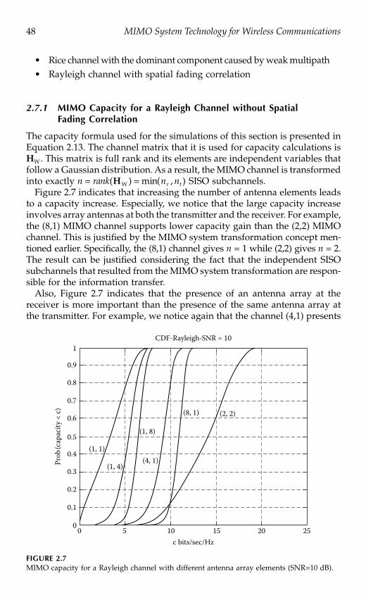
The capacity formula used for the simulations of this section is presented inEquation 2.13. The channel matrix that it is used for capacity calculations isHW. This matrix is full rank and its elements are independent variables thatfollow a Gaussian distribution. As a result, the MIMO channel is transformedinto exactly SISO subchannels.

Figure 2.7 indicates that increasing the number of antenna elements leadsto a capacity increase. Especially, we notice that the large capacity increaseinvolves array antennas at both the transmitter and the receiver. For example,the (8,1) MIMO channel supports lower capacity gain than the (2,2) MIMOchannel. This is justified by the MIMO system transformation concept men-tioned earlier. Specifically, the (8,1) channel gives n = 1 while (2,2) gives n = 2.The result can be justified considering the fact that the independent SISOsubchannels that resulted from the MIMO system transformation are respon-sible for the information transfer.

Also, Figure 2.7 indicates that the presence of an antenna array at thereceiver is more important than the presence of the same antenna array atthe transmitter. For example, we notice again that the channel (4,1) presents

FIGURE 2.7MIMO capacity for a Rayleigh channel with different antenna array elements (SNR=10 dB).

n rank n nr t= =( ) min( , )HW

1CDF-Rayleigh-SNR = 10

0.9

0.8

0.7

0.6

0.5

0.4

0.3

(1, 1)

(1, 4) (4, 1)

(1, 8)

(8, 1) (2, 2)

Prob

(cap

acity

< c)

0.2

0.1

00 5 10 15

c bits/sec/Hz 20 25



better capacity behavior than the channel (1,4). The explanation for this liesin the assumption that the transmitter does not have CSI, and as a result it“equi-powers” the elements regardless of the channel. On the contrary, thereceiver is considered to possess this information, and as a result it may useits antenna array for optimum combining based on CSI.

2.7.2 MIMO Capacity for a Rayleigh Channel with Spatial Fading Correlation

In this case the channel matrix is given by Equation 2.42. Figure 2.8 illustratesthe capacity for different antenna configurations and interelement spacingdistances, d in wavelengths.

Figure 2.8 proves the great effect of correlation to the MIMO channelcapacity. We can easily notice that the uncorrelated channel* (d = 0.5 ) offershigh capacity performance in comparison to rest cases. Specifically, theergodic capacity of the (4,4) uncorrelated channel is about 13 bits/sec/Hzgreater than the fully correlated one. So as the distance between the antennaelements decreases, the capacity decreases too. The reason lies in thecorrelation increase with the decrease of the interelement distance.Correlation between the transmitted and received signals decreases the

FIGURE 2.8CDFs of capacity for the Rayleigh MIMO channel with spatial fading correlation.

* We consider the scenario where half wavelength interelement distance introduces low enoughcorrelation that the fades can be considered independent [1].

1

0.9

0.8

0.7(2, 2)

CDF-correlated channel-SNR = 10

(4, 4)

0.6

0.5

0.4

0.3

Prob

(cap

acity

< c)

0.2

0.1

00 5 10 15 20 25 30

c bits/sec/Hz 35

d = 0.01 d = 0.1 d = 0.2 d = 0.5



independent propagation paths and, as a result, decreases the informationtransferred.

Also, we notice that the (4,4) MIMO channel achieves higher capacitycompared to the (2,2) channel, under any correlation conditions.

2.7.3 MIMO Capacity for a Ricean Channel

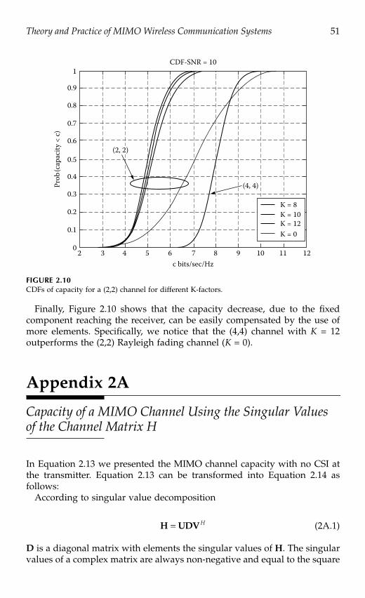
The channel matrix that it is used for capacity calculations is given byEquation 2.39. Figure 2.9 illustrates the CDFs of capacity for different antennaconfigurations and for a constant Ricean factor equal to K = 4. Figure 2.10illustrates the CDFs of capacity for a (2,2) MIMO channel for different Riceanfactors. The CDF for K = 0 represents the case of Rayleigh fading channel.

Apparently, Figure 2.9 indicates that the use of array antennas at both thetransmitter and receiver improves substantially the capacity. The same resultarose in the case of the simple Rayleigh channel studied in the previous section.

Figure 2.10 proves that the presence of a fixed component can cause greatdamage to the MIMO channel capacity performance. We easily see that thechannel capacity decreases when the Ricean factor increases. The value of Kcorresponds to the strength of the dominant component. As K increases, thedominant component appears stronger and the correlation coefficientincreases too. As mentioned before, correlation leads to the limitation of theindependent paths that transfer information and, hence, to lower capacitygains.

FIGURE 2.9CDFs of capacity for the Ricean MIMO channel with K = 4.

1

0.9

0.8

0.7

(2, 2)

(2, 4) (4, 2)

(4,4)

CDF-rank(HRice) = 1, SNR = 10, K = 4

0.6

0.5

0.4

0.3

Prob

(cap

acity

< c)

0.2

0.1

02 4 6 8 10 12

c bits/sec/Hz 14



Finally, Figure 2.10 shows that the capacity decrease, due to the fixedcomponent reaching the receiver, can be easily compensated by the use ofmore elements. Specifically, we notice that the (4,4) channel with K = 12outperforms the (2,2) Rayleigh fading channel (K = 0).

Appendix 2A

Capacity of a MIMO Channel Using the Singular Values of the Channel Matrix H

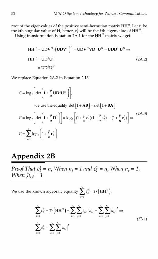
In Equation 2.13 we presented the MIMO channel capacity with no CSI atthe transmitter. Equation 2.13 can be transformed into Equation 2.14 asfollows:

According to singular value decomposition

(2A.1)

D is a diagonal matrix with elements the singular values of H. The singularvalues of a complex matrix are always non-negative and equal to the square

FIGURE 2.10CDFs of capacity for a (2,2) channel for different K-factors.

1

0.9

0.8

0.7

CDF-SNR = 10

0.6

0.5

0.4

0.3

Prob

(cap

acity

< c)

0.2

0.1

02 3 4 5 6 8 9 10 11 7

c bits/sec/Hz12

(2, 2)

(4, 4)

K = 8 K = 10 K = 12 K = 0

H UDV= H



root of the eigenvalues of the positive semi-hermitian matrix . Let k bethe kth singular value of H, hence, will be the kth eigenvalue of .

Using transformation Equation 2A.1 for the matrix we get:

(2A.2)

We replace Equation 2A.2 in Equation 2.13:

(2A.3)

Appendix 2B

Proof That 21 = nr When nt = 1 and 2

1 = nt When nr = 1, When �hi,j� = 1

We use the known algebraic equality :

(2B.1)

HHH

k2 HHH

HHH

HH UDV UDV UDV VD U UDD U

HH UD U

H H HH

H H H H H

H H

= ( ) = =

= 2

== UD U2 H

Cpn

H= +log det22I UD U ,

we use the equality det detI AB I B+ = + AA

I D= + = +Cpn

pn

log det log (22

2 1 12

22 2

2

1 1

1

)( ) ( )

log

+ +

= +

pn

pn

Cpn

n

k

k

n2

1=

k

k

nr

Tr2

1=

= ( )HHH

k

k

nH

i j i j

j

n

i

n

i

r tr

Tr h h h2

1 11= ==

= ( ) = =HH , , ,jj

j

n

i

n

k

k

n

i j

j

n

i

n

tr

r tr

h

2

11

2

1

2

11

==

= ==

= ,



When nt = 1, Equation 2B.1 gives:

(2B.2)

However, since nt = 1, and as a result there is only one .Hence, Equation 2B.2 takes the form:

(2B.3)

When nr = 1, Equation 2B.1 gives:

(2B.4)

Appendix 2C

Minimization of Angular Shift When R � d

In accordance with Figure 2.4, we denote the angular shift between theneighbor elements; this angle is given by the equation:

(2C.1)

where is the wavelength of the transmitted signal.From the figure above we have:

(2C.2)

substituting Equation 2C.2 into Equation 2C.1:

k

k

n

i j

ji

n

n

r r

rh2

1

2

1

1

1

12

22 2

= ==

= + + +, ... == nr

rank H( )HH = 1 k2 0

12 = nr

k

k

n

i j

j

n

i

t

r t

h n2

1

2

11

1

12

= ==

= =,

= =2 2R R

cf

R R

R R

Rd

Rd

Rd

=

=

=

=

cos

sin

cossin

sin



Assuming that or then approaches zero and we can use theapproximation:

(2C.4)

Finally, Equation 2C.3 is given by:

(2C.5)

Equation 2C.5 proves that under the aforementioned assumptions may beomitted from the matrix (Equation 2.38).

References

1. D.S. Shiu, J. Foschini, J. Gans, and J.M Kahn. 2000. “Fading correlationand its effect on the capacity of multielement antenna system,” IEEETransactions on Communications, 48, 502, 2000.

2. http://www.cs.ut.ee/~toomas_1/linalg/lin2/node14.html3. A. Paulraj, R. Nabar, and D. Gore. 2003. Introduction to Space-Time Wireless

Communications, Cambridge: Cambridge University Press, Chap. 4.4. I.E. Telatar, “Capacity of multi-antenna Gaussian channels,” Eur. Trans. Telecom.,

Vol. 10, No. 6, Dec. 1999.5. http://rkb.home.cern.ch/rkb/AN16pp/node123.html6. B.R. Ertel and P. Cardieri. 1998. “Overview of spatial channel models for an-

tenna array communication systems,” IEEE Personal Communication Magazine,Vol. 5, Feb. 1998, pp. 10–22.

7. G.V. Tsoulos and G.E. Athanasiadou. 2002. “On the application of adaptiveantennas to microcellular environments: radio channel characteristics andsystem performance,” IEEE Trans. Veh. Technol., Vol. 51, No. 1, Jan. 2002, pp.1–16.

8. G.E. Athanasiadou, A.R. Nix, and J.P. McGeehan. 2000. “A microcellular ray-tracing propagation model and evaluation of its narrowband and widebandpredictions,” IEEE J. Select. Areas Commun., Vol. 18, Mar. 2000, pp. 322–335.

= = =22 2R R d d d

sincos

sin11 2 2

2

4

2

=( )

=

cossin

sin

sin

sin

d

d22

2( )sin

(2C.3)

R d� d R� 1

sin = dR

= =44

12 2d d d

R�



9. G.E. Athanasiadou and A.R. Nix. 2000. “A novel 3D indoor ray-tracing prop-agation model: the path generator and evaluation of narrowband and wide-band predictions,” IEEE Trans. Veh. Technol., Vol. 49, July 2000, pp. 1152–1168.

10. 3GPP TR 25.996 V6.1.0 (www.3gpp.org).11. L. Correia, ed. 2001. Wireless Flexible Personalised Communications, New York:

Wiley.12. G.J. Foschini. 1996. “Layered space-time architecture for wireless communica-

tions in a fading environment when using multi-element antennas,” Bell LabsTech. J., Autumn 1996, pp. 41–59.

13. J.G. Proakis. 1983. Digital Communications, 4th ed., New York: McGraw-Hill,Chap. 2.

14. A. Papoulis. 1984. Probability, Random Variables, and Stochastic Processes, NewYork: McGraw-Hill.

15. M.A. Khalighi, J.-M. Brossier, G. Jourdain, and K. Raoof. 2001. “On capacity ofRicean MIMO channels,” in Proc. 12th IEEE Int. Symp. Personal, Indoor and MobileRadio Communications, A-150 to A-154, Vol. 1, 2001.

16. A. Zelst and J.S. Hammerschmidt. 2002. “A single coefficient spatial correlationmodels for multiple-input multiple output (MIMO) radio channels,” in Proc.URSI XXVIIth General Assembly, 2002.

17. S. Loyka and G.V. Tsoulos. 2002. “Estimating MIMO system performance usingthe Correlation matrix approach,” IEEE Commun. Letters, 6, 19, 2002.

18. J. Salz and J.H. Winters. 1994. “Effect of fading correlation on adaptive arrays indigital mobile radio,” IEEE Trans. Veh. Technol., Vol. 43, Nov. 1994, pp. 1049–1057.


MIMO System Technology for Wireless Communications

Documents

Transcript of MIMO System Technology for Wireless Communications