
MIMO in WCDMA and LTE - ST3...
74
MIMO in WCDMA and LTE LZT 123 9417 R1A © Ericsson 2009 - 1 - MIMO in WCDMA and LTE STUDENT BOOK LZT 123 9417 R1A
Transcript of MIMO in WCDMA and LTE - ST3...

MIMO in WCDMA and LTE
LZT 123 9417 R1A © Ericsson 2009 - 1 -
MIMO in WCDMA and LTE
STUDENT BOOK LZT 123 9417 R1A

MIMO in WCDMA and LTE
- 2 - © Ericsson 2009 LZT 123 9417 R1A
DISCLAIMER This book is a training document and contains simplifications. Therefore, it must not be considered as a specification of the system. The contents of this document are subject to revision without notice due to ongoing progress in methodology, design and manufacturing. Ericsson assumes no legal responsibility for any error or damage resulting from the usage of this document. This document is not intended to replace the technical documentation that was shipped with your system. Always refer to that technical documentation during operation and maintenance.
© Ericsson 2009 This document was produced by Ericsson. • It is used for training purposes only and may not be copied or
reproduced in any manner without the express written consent of Ericsson.
This Student Book, LZT 123 9417, R1A supports course number LZU 108 7652 .

Table of Contents
LZT 123 9417 R1A © Ericsson 2009 - 3 -
Table of Contents
1 MIMO INTRODUCTION.................................................................5 OBJECTIVES:...................................................................................................5
INTRODUCTION....................................................................................7 MIMO BASICS ..................................................................................................7
2 RADIO CHANNEL AND ANTENNA BASICS .............................13 OBJECTIVES:.................................................................................................13
BASIC RADIO CHANNEL PROPERTIES ...........................................15
ANTENNA BASICS..............................................................................26 PRACTICAL IMPLEMENTATION OF ANTENNAS FOR MIMO .....................29
3 PRECODING AND SPATIAL MULTIPLEXING...........................35 OBJECTIVES:.................................................................................................35
PRECODING FOR SPATIAL MULTIPLEXING, TX DIVERSITY AND BEAMFORMING .........................................................................37 SPATIAL MULTIPLEXING ..............................................................................39
4 MIMO IN WCDMA........................................................................45 OBJECTIVES:.................................................................................................45
MIMO IN WCDMA................................................................................47
5 MIMO IN LTE...............................................................................57 OBJECTIVES:.................................................................................................57
MIMO IN LTE........................................................................................59

MIMO in WCDMA and LTE
- 4 - © Ericsson 2009 LZT 123 9417 R1A
Intentionally Blank
1 MIMO Introduction
LZT 123 9417 R1A © 2009 Ericsson - 5 -
1 MIMO Introduction
OBJECTIVES:
On completion of this chapter the student will be able to:Describe the basics of MIMO
– Explain the reason for multi-antenna processing– List the different methods of multi-antenna processing – Explain the different multi antenna possibilities– Explain the general concepts of beamforming, diversity and
spatial multiplexing– Explain the concepts of MIMO, SIMO, MISO and SISO
Figure 1-1 Objectives
MIMO in WCDMA and LTE
- 6 - © Ericsson 2009 LZT 123 9417 R1A
Intentionally Blank

1 MIMO Introduction
LZT 123 9417 R1A © 2009 Ericsson - 7 -
INTRODUCTION Multiple antenna solutions can be used in order to increase the spectrum efficiency as well as the peak data rates. Different approaches aim for different purposes, e.g. traditional beamforming and transmitter diversity techniques increase the coverage and capacity. Spatial multiplexing, a technique which requires multiple antennas at both transmitter and receiver, increases the peak data rates and spectrum efficiency up to several hundred percent.
Advanced antenna solutions– Tx & Rx Diversity– Multi-layer transmission (Spatial Multiplexing)– Beam-forming
TX TXTX TX
Figure 1-2. Multi antenna features.
MIMO BASICS
The use of multiple antennas relies on two different principles • Improving the SNR (Signal to Noise Ratio)
• Sharing the SNR
This means that in scenarios where the SNR is low, improving the SNR is the way to go. This can be achieved by the use of beamforming, tx diversity and/or rx diversity.
Beamforming concentrates the transmitted (and/or received) energy in desired direction(s).
MIMO in WCDMA and LTE
- 8 - © Ericsson 2009 LZT 123 9417 R1A
Tx diversity achieves diversity against the channel fading by transmitting the information at different times and/or from different antenna locations. Open Loop tx diversity does not exploit any channel information (no feedback from receiver) while closed loop tx diversity uses feedback from the UE in order to maximize the performance.
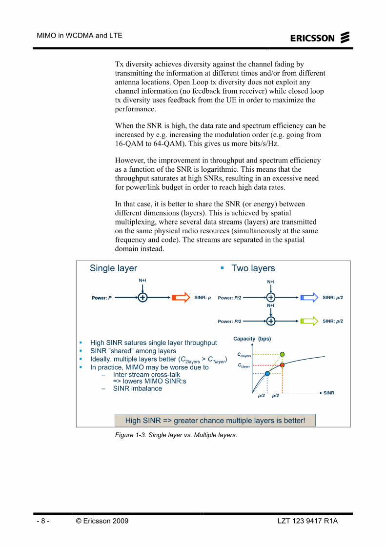
When the SNR is high, the data rate and spectrum efficiency can be increased by e.g. increasing the modulation order (e.g. going from 16-QAM to 64-QAM). This gives us more bits/s/Hz.
However, the improvement in throughput and spectrum efficiency as a function of the SNR is logarithmic. This means that the throughput saturates at high SNRs, resulting in an excessive need for power/link budget in order to reach high data rates.
In that case, it is better to share the SNR (or energy) between different dimensions (layers). This is achieved by spatial multiplexing, where several data streams (layers) are transmitted on the same physical radio resources (simultaneously at the same frequency and code). The streams are separated in the spatial domain instead.
High SINR satures single layer throughputSINR ”shared” among layersIdeally, multiple layers better (C2layers > C1layer)In practice, MIMO may be worse due to
– Inter stream cross-talk=> lowers MIMO SINR:s
– SINR imbalance
SINR: ρPower: PPower: P
N+I
SINR: ρ/2Power: P/2
N+I
SINR: ρ/2Power: P/2
N+I
Single layer Two layers
Capacity (bps)
ρ/2 ρ/2
C1layer
C2layers
SINR
High SINR => greater chance multiple layers is better! Figure 1-3. Single layer vs. Multiple layers.

1 MIMO Introduction
LZT 123 9417 R1A © 2009 Ericsson - 9 -
The data rate only increases logarithmically as a function of the SNR (or SINR – Signal to Interference and Noise Ratio), at a high SNR. This is according to the Shannon theorem
rdata = BW x log2(1+SNR)
(max data rate rdata is equal to the bandwidth, BW, multiplied by the base-2 logarithm of the SNR plus 1).
On the other hand, at a low SNR, the max data rate increases almost linearly. Therefore, it is not efficient aiming only to obtain a high SNR. It is more efficient to try to create several “data pipes” with lower SNR (sharing SNR), which will lead to a multiplication of the maximum achievable data rate with up to the channel rank rmax.
With MIMO
Multistream Rx/Tx processing,Multiple Rx and Tx antennas
Share SNR between streams ⇒Linear increase in rate
Without MIMO
Single stream Rx/Tx processing,Multiple Rx and/or Tx antennas
Low SNR: approx linear increase in rateHigh SNR: logarithmic increase in rate
Cmimo ∼N x log(1+SNR)C ∼log(1+N x SNR)C ∼log(1+N x SNR)
SNR
Cap
SNR N x SNR
SNR
Cap
SNR N x SNR
C ∼log(1+SNR)
SNR
Cap
SNR N x SNR
SNR
Cap
SNR N x SNR
Figure 1-4. Why MIMO?
A traditional way of sharing the SNR is actually by spread spectrum techniques, e.g. CDMA, where the transmission is multiplexed over a wider bandwidth.
Different configurations of multiple antennas are shown in Figure 1-5. These include SISO (Single Input Single Output), MISO (Multiple Input Single Output), SIMO (Single Input Single Output) and of course, MIMO (Multiple Input Multiple Output). The naming convention refers to input/output of the radio channel. This means that the transmitter antenna(s) correspond to input to the radio channel and the receiver antenna(s) reception correspond to the output of the radio channel.

MIMO in WCDMA and LTE
- 10 - © Ericsson 2009 LZT 123 9417 R1A
S-PRXRXTX
SISO
RXRX
MISO
S-P
MIMO
RXS-P
MIMO
RXRXRXRXTX
SIMO
Figure 1-5. Antenna configurations.
With multiple antennas at the transmitter and only single antenna at the receiver (referred to as MISO) it is possible to obtain so called beamforming. With this method the transmission signal is steered in a beneficial direction (typically towards the UE). This is accomplished by adjusting the phase (and sometimes amplitude) of the different antenna elements by multiplying the signal with complex weights. This method increases the SNR (Signal to Noise Ratio) and thus the capacity.
With this configuration it is also possible to achieve Transmit Diversity. This is done by transmitting time-shifted copies of the signal and thus achieving diversity in the time-domain. This method also increases the SNR.
With multiple antennas at the receiver (SIMO or MIMO), it is possible to use receive diversity. A combining method (typically MRC – Maximum Ratio Combining) is applied to increase the SNR of the received signal.
With multiple antennas at both transmitter and receiver, it is possible to use all of the above mentioned methods.
However, with multiple antennas at both transmitter and receiver, it is also possible to achieve spatial multiplexing, also referred to as MIMO. This method creates several layers, or “data pipes” in the radio interface. The maximum number of layers that can be created depends on the radio channel characteristics and the number of tx and rx antennas. The maximum number of layers that the radio channel can support is equal to the channel rank. The maximum number of layers that effectively can be used is equal or less than the minimum number of antenna elements at the tx or rx side or the channel rank. The number of layers that actually is used for transmission is referred to as the transmission rank.

1 MIMO Introduction
LZT 123 9417 R1A © 2009 Ericsson - 11 -
The data rate can at optimal circumstances be multiplied by the number of layers.
Diversity“Reduce fading”
Example
Transmit the signal in all Transmit the signal in all directionsdirections
Diversity“Reduce fading”
Example
Transmit the signal in all Transmit the signal in all directionsdirections
Spatial Multiplexing“Data Rate multiplication”
Example
Transmit several signals in Transmit several signals in different directionsdifferent directions
Spatial Multiplexing“Data Rate multiplication”
Example
Transmit several signals in Transmit several signals in different directionsdifferent directions
S-PS-PDela
yDela
y
DirectivityAntenna/Beamforming gain
Example
Transmit the signal in the Transmit the signal in the best directionbest direction
DirectivityAntenna/Beamforming gain
Example
Transmit the signal in the Transmit the signal in the best directionbest direction
Channel knowledge (average/instant)
• Different techniques make different assumptions on channel knowledge at rx and tx• Many technqiues can realize several benefits• Realized benefit depends on channel (incl. antenna) and interference properties
Figure 1-6. Multi-antenna possibilities.
Better data rate coverage and capacity– Directivity and diversity improves link budget
Potential for higher data rates– Spatial domain provides extra dimension
Extra dimension offers increased data ratesIdeally: rmax times higher data rate than single Tx(rmax = min#tx antennas, #rx antennas)
Transmit r ≤ rmax parallel symbol streams (layers)Max rmax parallel ”data pipes”Number of layers r depends on channel properties
– Channel rank r: #effective data pipes channel can support(data pipes with sufficiently strong SINR)
Rank adaption dynamically adjusts #layers
Higher spectral efficiency!
Up to rmax times higher throughput! Figure 1-7. Possible multi-antenna benefits.
In a simple beamforming example, the complex weights are adjusted in order to align the carrier phase in such a way that the individual antenna elements’ signals are added constructively at the receiver side. With two antenna elements we need two complex weights, here denoted w1 and w2. These weights are adjusted with the support of some kind of feedback from the receiver (in this case the UE), in order to maximize the reception.

MIMO in WCDMA and LTE
- 12 - © Ericsson 2009 LZT 123 9417 R1A
With multiple antennas (here called antenna ports) at both tx and rx side and multiple layers, the complex weights will form a matrix. In case of 4x4 MIMO and four layers, a 4x4 matrix will be needed. This means that each layer will have its own complex weight vector of length equal to the number of antenna elements.
Adapt spatial properties of transmission to match current channel conditionsPrecoding/beamforming example
Coherent addition of signals at receive side increases SNRSimilar to closed-loop TxD in WCDMAPrecoding with multi layers
– Multiply each layer with corresponding precoding vector=> matrix weighting!
w1
w2
sh2
h1
y = (h1w1 + h2w2)s + e
Figure 1-8. Precoding for exploiting channel info at tx side.

2 Radio Channel and Antenna basics
LZT 123 9417 R1A © 2009 Ericsson - 13 -
2 Radio Channel and Antenna basics
OBJECTIVES:
On completion of this chapter the student will be able to:
Describe the radio channel and antenna basics– Explain multi-path propagation– Explain time dispersion and delay spread– Explain the doppler effect– Explain coherence bandwidth and coherence time– Explain DOA (Direction of Arrival) DOD (Direction of Departure)
and angular spread– Explain polarization properties of the radio channel– Explain basic antenna properties – Explain polarization properties of antennas– Describe beamforming using an ULA (Uniform Linear Array) – Explain polarization diversity
Figure 2-1. Objectives.

MIMO in WCDMA and LTE
- 14 - © Ericsson 2009 LZT 123 9417 R1A
Intentionally Blank

2 Radio Channel and Antenna basics
LZT 123 9417 R1A © 2009 Ericsson - 15 -
BASIC RADIO CHANNEL PROPERTIES In order to understand the principles of MIMO and spatial division multiplexing (SDM) and spatial division multiple access (SDMA), the radio channel properties is first explained below.
The radio channel distorts the transmitted signal between the transmitter and the receiver. This distortion is due to various reasons. For example, the original signal is added with noise and interference, distorted by Doppler shift, time dispersion and frequency selective fading.
Noise and interference– Reduced coverage and quality
Fading (fast and slow)– Fluctuating signal strength
Time dispersion– Inter symbol interference (ISI) and fast fading
Doppler shift– Frequency errors and reduced performance
Noise
Interference Time dispersion
Doppler shift
Radio channelFast Fading
Transmission
Slow Fading
Figure 2-2. Radio channel impairments.
Noise and interference
Noise can be divided into internal noise and external noise. Internal noise originates from the system itself, especially from the receiver circuitry. This noise is to a large extent coming from the first amplifier in the receiver. The quality of this amplifier judges the amount of thermal noise added from the amplifier itself. The lower noise factor (NF) the amplifier has, the less noise will be added. This is the reason why we call it LNA (Low Noise Amplifier).
External noise comes from other systems, the surrounding environment, galactic noise etc.
MIMO in WCDMA and LTE
- 16 - © Ericsson 2009 LZT 123 9417 R1A
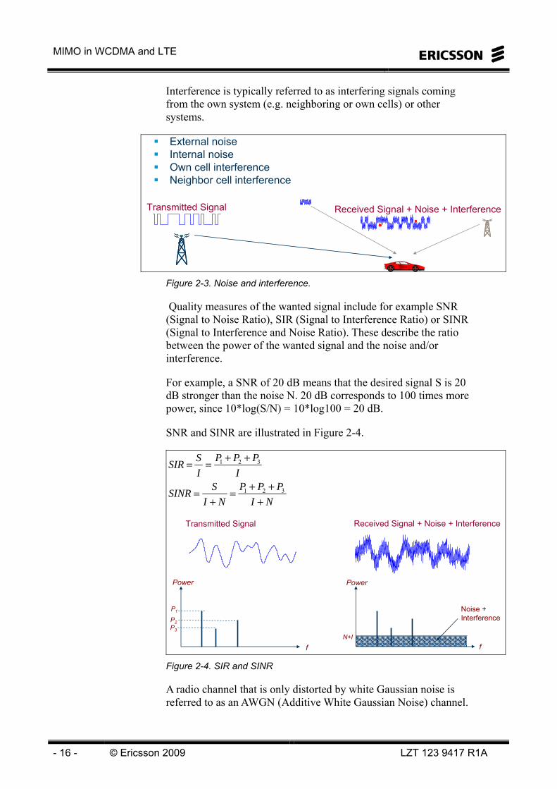
Interference is typically referred to as interfering signals coming from the own system (e.g. neighboring or own cells) or other systems.
External noiseInternal noiseOwn cell interferenceNeighbor cell interference
Transmitted Signal Received Signal + Noise + Interference
Figure 2-3. Noise and interference.
Quality measures of the wanted signal include for example SNR (Signal to Noise Ratio), SIR (Signal to Interference Ratio) or SINR (Signal to Interference and Noise Ratio). These describe the ratio between the power of the wanted signal and the noise and/or interference.
For example, a SNR of 20 dB means that the desired signal S is 20 dB stronger than the noise N. 20 dB corresponds to 100 times more power, since 10*log(S/N) = 10*log100 = 20 dB.
SNR and SINR are illustrated in Figure 2-4.
Transmitted Signal Received Signal + Noise + Interference
Noise +Interference
f f
Power Power
P1
P2P3
N+I
NIPPP
NISSINR
IPPP
ISSIR
+++=
+=
++==
321
321
Figure 2-4. SIR and SINR
A radio channel that is only distorted by white Gaussian noise is referred to as an AWGN (Additive White Gaussian Noise) channel.

2 Radio Channel and Antenna basics
LZT 123 9417 R1A © 2009 Ericsson - 17 -
Multipath propagation
When the signal bounces on different obstacles in the environment, different time delayed copies with different powers will reach the receiver. This is referred to as multipath propagation.
Multipath propagation gives rise to • Fading (fast fading, Rayleigh fading)
• Time dispersion (Inter Symbol Interference, ISI)
Many radio propagation effects such as reflections can attenuate the transmitted radio signal Figure 2-5.
Figure 2-5: Multipath Propagation. The received signal contains many time-delayed replicas.
τ0 τ1 τ2 t(μs)
P0
P1
P2
Power (dB)
P2,τ2
P0,τ0 P1,τ1
Multipath Propagation gives rise to:
1. InterSymbol Interference (ISI)
2. Fast fading (Rayleigh fading)
Impulse response
Figure 2-6. Multipath propagation and the resulting impulse response.

MIMO in WCDMA and LTE
- 18 - © Ericsson 2009 LZT 123 9417 R1A
This occurs when the propagation wave reflects on an object, which is large compared to the wavelength, for example, the surface of the earth, buildings, walls, etc. This phenomenon is called multipath propagation and it has several effects, these are:
• Rapid changes in signal strength over a small area or time interval
• Random frequency modulation due to varying Doppler shifts on different multipath signals.
• Time dispersion caused by multipath propagation delays
Previous symbol leaks into current symbol due to the different path delaysWhen the amount of ISI exceeds a certain level (~10%) bit errorsoccurCan be reduced with equalizers, rake receivers or the use of OFDM
Direct signal
Reflected signal
Path delay difference
ISI
Figure 2-7 Inter Symbol Interference (ISI).
Multipath propagation yields signal paths of different lengths with different times of arrival at the receiver. Typical values of time delays (µs) are 0.2 in Open environment, 0.5 Suburban and 3 in Urban.
Direct S ignal
Reflected Signal
Com bined S ignal
Figure 2-8: Multipath Fading.
2 Radio Channel and Antenna basics
LZT 123 9417 R1A © 2009 Ericsson - 19 -
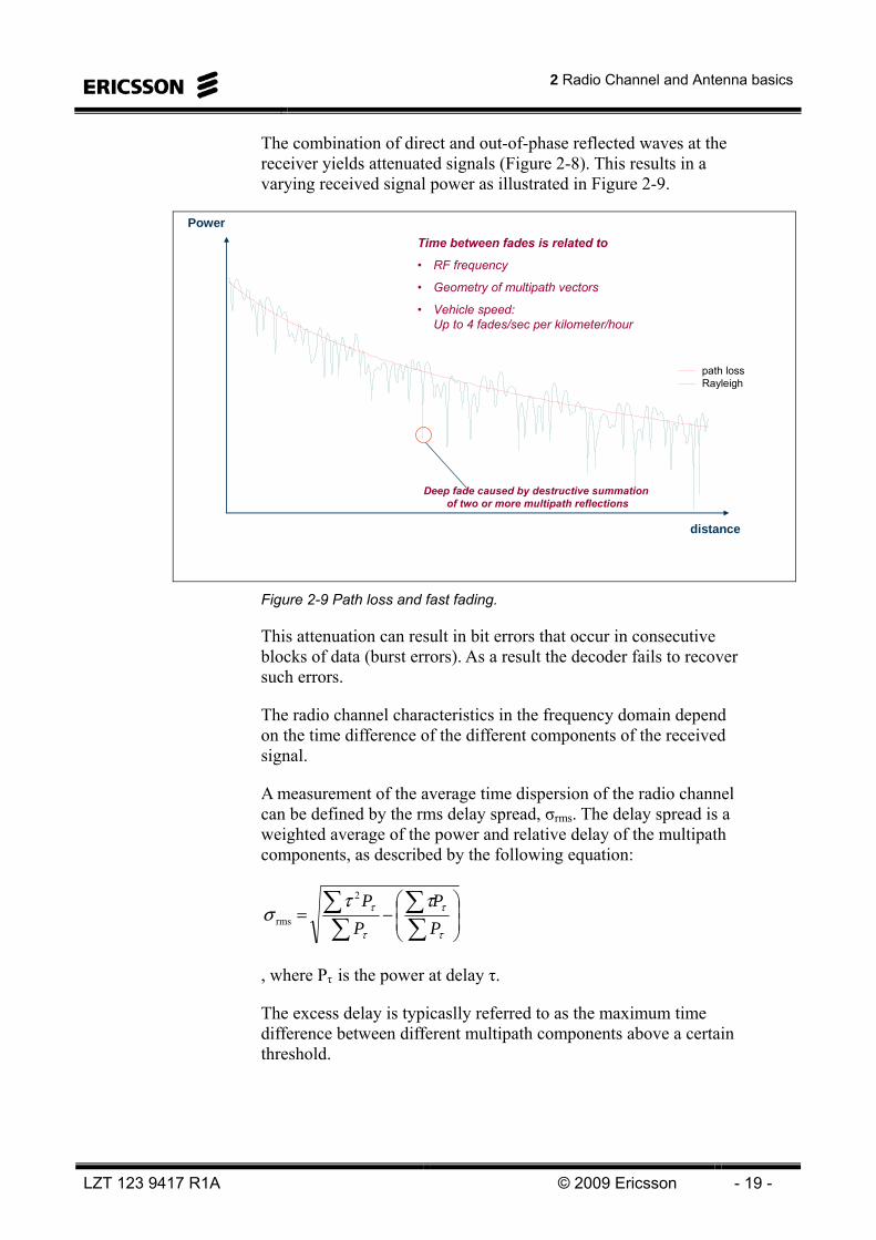
The combination of direct and out-of-phase reflected waves at the receiver yields attenuated signals (Figure 2-8). This results in a varying received signal power as illustrated in Figure 2-9.
Power
distance
Time between fades is related to
• RF frequency
• Geometry of multipath vectors
• Vehicle speed: Up to 4 fades/sec per kilometer/hour
path lossRayleigh
Deep fade caused by destructive summationof two or more multipath reflections
Figure 2-9 Path loss and fast fading.
This attenuation can result in bit errors that occur in consecutive blocks of data (burst errors). As a result the decoder fails to recover such errors.
The radio channel characteristics in the frequency domain depend on the time difference of the different components of the received signal.
A measurement of the average time dispersion of the radio channel can be defined by the rms delay spread, σrms. The delay spread is a weighted average of the power and relative delay of the multipath components, as described by the following equation:
⎟⎟⎠
⎞⎜⎜⎝
⎛−=∑∑
∑∑
τ
τ
τ
τ ττσ
PP
PP2
rms
, where Pτ is the power at delay τ.
The excess delay is typicaslly referred to as the maximum time difference between different multipath components above a certain threshold.

MIMO in WCDMA and LTE
- 20 - © Ericsson 2009 LZT 123 9417 R1A
On average, the coherence bandwidth is equal to the inverse of the delay spread.
rmsCB
σ1=
The coherence bandwidth defines how frequency selective the radio channel is. For example, a coherence bandwidth higher than the transmitted bandwidth (which typically occurs when the delay spread is shorter than the symbol time) will give almost flat fading. Flat fading means that the whole transmitted bandwidth fades equally, or in other words, the correlation between all frequencies in the transmitted bandwidth is high.
Coherence BW > Tx BW:– The transmission experiences almost flat fading– Only frequency hopping and/or Antenna diversity (Tx & Rx diversity,
beamforming, SM) can reduce and even exploit the fading
Coherence BW < Tx BW:– FEC can reduce the errors caused by fading– Frequency hopping and/or Antenna diversity (Tx & Rx diversity, beamforming,
SM) can further reduce and exploit the fading
fTx BW
fTx BW
Large Coherence BW
Low Coherence BWP
P
Figure 2-10. Coherence bandwidth.
Tx (and Rx) diversity and beamforming can reduce the fading by exploiting the differences between the antenna elements.
MIMO with spatial multiplexing can reduce and even exploit the fading by amplifying wanted paths and cancelling unwanted paths in the spatial domain by altering the antenna phases.

2 Radio Channel and Antenna basics
LZT 123 9417 R1A © 2009 Ericsson - 21 -
The time varying radio channel
When the terminal is moving, the radio channel properties will change locally. However, the long term statistics of the channel will typically remain the same on average, e.g. delay spread, coherence bandwidth etc. This is referred to as a WSSUS (Wide Sense Stationary Uncorrelated Scattering) channel.
As the terminal moves, the fast fading has a large impact on the received signal strength. Locally, the signal strength may vary as much as 40 dB (10000 times) due to Rayleigh fading. Rayleigh fading typically occurs when a large number (>10) of uncorrelated signal components are added. This is actually the normal case in urban environments.
Another phenomenon that occurs due to mobility is Doppler shifts. When the terminal is moving towards the transmitter/receiver (base-station), the carrier frequency is slightly increased and vice-versa. The Doppler shift is equal to the speed divided by the wavelength of the carrier signal. This ratio is valid when the terminal is moving straight towards the transmitter. When moving in a certain angle α towards the transmitter, the following equation is valid.
( )αλ
cos⋅= vfd
The inverse of the average Doppler spread is equal to the coherence time of the radio channel. The coherence time describes how slowly the radio channel changes.
( )αλ
cos1
⋅==
vfT
dC
A high coherence time means that the radio channel does not change rapidly.
The symbol time should typically be shorter than the coherence time. Otherwise the symbols become distorted.
In order for MIMO in e.g. LTE to work well, the symbol time should be long enough in order to experience flat fading, but should at the same time not exceed the coherence time of the channel. Also, the feedback from the terminal must be quick and fresh enough so that the radio channel properties have not changed too much when the signal is transmitted.

MIMO in WCDMA and LTE
- 22 - © Ericsson 2009 LZT 123 9417 R1A
The spatio-temporal radio channel
An actual radio channel has certain properties in the spatial domain as well as in the temporal (time) domain.
In the spatial domain, the channel can be described in terms of e.g. angular spread of DOA (Direction Of Arrival) and DOD (Direction Of Departure). The angular spread is a weighted average of the DOA or DOD of the radio channel. Typically, the angular spread can be quite low at the base-station (especially if it is mounted on a roof top). The UE will typically have a larger angular spread, since the reflections often comes from objects surrounding the UE in almost all directions.
Angular spread at base station side typically much lower than at the terminal side– Beamforming at base station side beneficial– Easier to obtain low spatial correlation at terminal side (shorter antenna distance
than at base station)
Angular spread low
Angular spread high
Figure 2-11. Angular spread in a typical urban scenario.
The angular spread AS can be calculated in a similar manner as the delay spread, i.e.:
⎟⎟⎠
⎞⎜⎜⎝
⎛−=∑∑
∑∑
τ
τ
τ
τ ϕϕPP
PP
AS2
rms
, where φ is the azimuth angle of each multipath component.
With a high angular spread, the antenna elements become more un-correlated, given that they are separated in the same dimension as the angular spread. For example, if the azimuth angular spread is high, then the antenna elements become quite un-correlated even if the separation in the horizontal plane is quite small.
In the temporal domain, the channel can be described in terms of e.g. delay spread, excess delay and coherence time.

2 Radio Channel and Antenna basics
LZT 123 9417 R1A © 2009 Ericsson - 23 -
Polarization
The radio signal can be transmitted with different polarizations. The polarization is defined by the direction of the electrical field vector (E-field). Orthogonal polarizations, such as e.g. horizontal/vertical or ±45°, makes it possible to transmit and receive two different data streams independent of each other on the same frequency at the same time. However, the radio channel usually alters the polarizations so they will interfere with each other. Also, a typical cross polarized antenna will not separate the different polarizations perfectly. The separation depends on the antennas XPD (Cross Polarization Discrimination). A typical value of XPD is approximately 20 dB (100 times in power),
Vertical:Full reception
Horizontal:No reception
Receiver antenna polarization:
The electrical field (E-field) determines the polarization
E
E
E
Vertical transmitter antenna polarization:
Figure 2-12. Example of linear vertical polarization.
As opposite to linear polarization, circular and elliptical polarization also exists. With circular polarization, the E-field rotates in a circle (constant amplitude), either clockwise (right hand circular polarization) or anti-clockwise (left hand circular polarization), when viewed along the propagation path as seen from the transmitter. With elliptical polarization, the vector describes an ellipsoid.

MIMO in WCDMA and LTE
- 24 - © Ericsson 2009 LZT 123 9417 R1A
Can be created by two perpendicular linearlypolarized antenna elements fed with different phases
Figure 2-13. Circular polarization.
Figure 2-14 gives a more detailed illustration of circular polarization.
”Right-hand circular” polarized current sourceTwo orthogonal dipoles in phase quadrature
– Horizontal and vertical
When the plane of polarization is viewed in the direction of propagation at a fixed point in space, if the extremes of the E-field vector describes a
circle and rotates clockwise as a function of time, the sense is right-hand circular (RHC).
Figure 2-14. Antenna polarization.
Circular polarization may very well be utilized in cellular systems. The benefit is that the transmission will be more independent of the UE position (the base station has no way of knowing the polarization of the UE antenna(s)). The drawback is that there will be a loss (compared to perfectly co-polarized tx and rx antennas) of 3dB.

2 Radio Channel and Antenna basics
LZT 123 9417 R1A © 2009 Ericsson - 25 -
Reciprocity
The radio channel is reciprocal, meaning that the properties of the radio channel are the same, regardless of the direction (UL or DL) of the transmissions. This means that properties like impulse response, delay spread, azimuth spread, fading etc are the same in both UL and DL. This assumes that the same frequency band is used for both UL and DL (as in the TDD mode, for example) and that that the transmissions are performed at the same time. Since this almost never happens, a more loose definition can be used. A radio channel could for example be regarded as more or less reciprocal if the duplex distance is shorter than the coherence bandwidth and/or the time between UL/DL transmissions is less than the coherence time of the radio channel.

MIMO in WCDMA and LTE
- 26 - © Ericsson 2009 LZT 123 9417 R1A
ANTENNA BASICS The simplest example of an antenna is probably the half-wavelength dipole. It consists of a “rod”, which is split and fed with the carrier wave. The electrical current in the antenna element creates an electrical and a magnetic field that propagates from the antenna. The electrical field and the magnetic field vectors are perpendicular.
An antenna can be seen as a matching of the wave impedances between the antenna feeder (often 50Ω) and “the surroundings” (free space) of the antenna. The free space impedance is by definition the ratio between the electrical field and the magnetic field absolute values. This wave impedance equals 377 Ω. At a perfect match, no energy is reflected from the antenna back to the transmitter.
The half-wavelength dipole has an omni-directional radiation pattern in the azimuth plane. In the elevation plane the radiation pattern is slightly directed perpendicularly from the antenna element. In the direction of the antenna “rod” the radiation is zero. See figure Figure 2-15.
Omni-directional radiation pattern(Doughnut-shape)
Eλ/2
- omni horizontal coverage- wide vertical coverage- low gain
Figure 2-15. The classical half wavelength dipole.
The electrical field from the half wavelength dipole is aligned with the direction of the “rod” (vertical in Figure 2-15).

2 Radio Channel and Antenna basics
LZT 123 9417 R1A © 2009 Ericsson - 27 -
Antenna arrays and beamforming
When two or more antenna elements are used for transmission or reception (the antennas are also reciprocal), their respective signals will be summed. The resultant signal vector will depend on their relative position, phase, and the direction of the transmitter/receiver. Also, the polarization will affect this summation. In some directions we will see amplification of the resultant signal and in other directions we will see cancellation (nulls). This is referred to as the array factor. The array factor can be multiplied with the antenna element’s radiation pattern in order to obtain the resulting array pattern. If the individual antenna element’s radiation pattern is omni-directional (in e.g. the azimuth plane), the resulting diagram will equal the array factor.
The most common way of implementing an antenna array for beamforming is by the use of a ULA (Uniform Linear Array), consisting of (cross-polarized) dipoles. The antenna elements (dipoles) will add constructively at certain directions, depending on the geometry of the array and the individual phases of the signals fed to the different elements.
When stacking columns of elements horizontally, it is possible to steer the antenna beam in the azimuth (horizontal) plane. The horizontal distance between the elements should be in the order of half a wavelength in order to avoid grating lobes (unwanted sidelobes).
∆x )sin(α⋅=Δ dx
d d
∆x
αα
Figure shows a 4-element Uniform Linear Array (ULA) When ∆x is λ/2 we have nulls (assuming signals to the different elements in phase)Antenna element distance of d=λ/2 eliminates grating lobes
Figure 2-16. Uniform Linear Array (ULA).

MIMO in WCDMA and LTE
- 28 - © Ericsson 2009 LZT 123 9417 R1A
When the inter-element distance exceeds half a wavelength, grating lobes are created.
With a larger antenna element distance, the main lobe is narrower, but unwanted sidelobes (grating lobes) are created
d=0.63λ d=0.5λ
d
Figure 2-17. Main lobes and grating lobes.
When the inter-antenna element distance is approximately one wavelength, the grating lobes become as strong as the main lobes. When increasing the antenna distance further, several lobes with the same strength are created. This may sometimes be beneficial when used with spatial multiplexing.
More ”main lobes” are created if the antenna distance exceeds approximately half a wavelength
d = 0.5 wavelengths d = 1.0 wavelengths
d d
Figure 2-18. Two element array radiation pattern.

2 Radio Channel and Antenna basics
LZT 123 9417 R1A © 2009 Ericsson - 29 -
PRACTICAL IMPLEMENTATION OF ANTENNAS FOR MIMO
How can we practically implement an antenna configuration for MIMO? Well, a suitable way of achieving uncorrelated antenna elements is to use polarization diversity with cross-polarization. 2x2 MIMO can quite easily be configured with existing cross-polarized antennas. This works well even in line-of-sight (LOS) environments (4x4 MIMO may actually perform worse in a LOS environment than in a non-LOS environment, since the LOS environment probably lack the useful multi-path diversity and we only have two orthogonal polarizations). A four antenna-port configuration can be realized using two cross-polarized antennas.
Many different possible antenna configurations– Only two different ones considered here
Exploit orthogonal polarizations– Reduces inter-layer interference– Dual-layer transmission possible also in line-of-sight– Line-of-sight not uncommon in urban environments
Two cross-polarized antennas
Two pairs of cross-polarized antennas– Dual stream spatial multiplexing– Array gain by means of beamforming on pairs of co-polarized antennas– Limited radome size
0.5λ Figure 2-19. Antenna setup at the base station.
Figure 2-20 shows a Kathrein cross-polarized, stacked dipole antenna.
Kathrein 800 10204– 900 MHz
Linear array– seven dipole pairs
~0.95 λ (wavelengths) apart
Figure 2-20. Linear cross polarized array antenna.

MIMO in WCDMA and LTE
- 30 - © Ericsson 2009 LZT 123 9417 R1A
The cross polarized antenna elements work in pairs, as illustrated in Figure 2-21.
Basic building block: Dipole over ground plane– Two per polarization Pol. 1: - 45˚
Pol. 2: + 45˚
λ/2
Figure 2-21. Cross polarized dipole antennas.
MIMO channel properties affecting the choice of transmission scheme
The propagation environment obviously affects the properties of the MIMO channel via many factors including mobility, path loss, shadow fading, polarization, angular spread of direction of departures (DOD) and arrivals (DOA). This in combination with the particular antenna setup at the transmitter and receiver determines the channel characteristics. Some of the key parameters regarding an idealized antenna setup are • Distances between antennas within the arrays
• Polarization of the antennas
Basically, a larger inter-antenna distance gives less correlated channel for a given fixed angular spread and vice versa. Signals transmitted with horizontal and vertical polarization tend to experience uncorrelated fading and this can also be exploited to reduce spatial correlation if so desired. Another important characteristic of transmitting some signals with horizontal polarization and other with vertical polarization is that often the two orthogonal polarizations remain rather well separated even after reaching the receiver. Under ideal conditions in line-of-sight, they would for example be completely separated. Thus, varying inter-antenna distances and polarization can be used to affect the spatial correlation and the isolation between signals.

2 Radio Channel and Antenna basics
LZT 123 9417 R1A © 2009 Ericsson - 31 -
Since a transmission scheme usually work well in a channel with certain properties and less well with other properties, the antenna setup greatly affects which transmission scheme to choose, and vice verse. The previously mentioned transmission schemes are targeting different channel characteristics and hence are suitable together with different antenna setups. Some of the more obvious possible combinations under idealized assumptions regarding the antennas are listed below
• Beamforming:
o Strong spatial correlation on the transmitter side meaning
small inter-antenna distance and co-polarized antennas on transmit side
• Transmit diversity, e.g. the Alamouti code:
o Low spatial correlation on at least the transmitter side achieved by either of
co-polarized antennas on both transmit and receive side with large inter-antenna distance on transmit side
orthogonally polarized antennas on transmit side and receive side
• SU-MIMO spatial multiplexing:
o Low spatial correlation on both the transmit and receive side and/or good isolation between different transmit-receive antenna pairs provided by either
co-polarized antennas on both transmit and receive side with large inter-antenna distances on both sides
orthogonally polarized antennas on transmit side and receive side

MIMO in WCDMA and LTE
- 32 - © Ericsson 2009 LZT 123 9417 R1A
Beamforming: – Small inter-antenna distance and co-polarized antennas on
tx side
Transmit diversity, e.g. the Alamouti code: – Co-polarized antennas on both tx and rx side with large
inter-antenna distance on tx side– Orthogonally polarized antennas on tx side and rx side
SU-MIMO spatial multiplexing: – Co-polarized antennas on both tx and rx side with large
inter-antenna distances on both sides – Orthogonally polarized antennas on tx side and rx side
Figure 2-22. Antenna configurations
Note that the meaning of “large” and “small” should be interpreted relative to the angular spread on the intended side of the link. For a base station mounted above roof tops the angular spread might for example be quite small and “small” may then be taken as half a wavelength and “large” might be 4-10 wavelengths while on the UE side, which typically experiences a much larger angular spread, half a wavelength might be considered “large”.
Reality is unfortunately not as idealized as indicated above, but the list still gives guidance as to which kind of antenna setups the different schemes prefer. In practice, it is for example difficult to guarantee co-polarized antennas on both transmit and receive side simply because the user might have rotated the device. In the UE, it is often also challenging to design purely co-polarized or purely orthogonally polarized antennas, due to for example form factor requirements and RF interactions. Antenna design is an interesting and important topic that clearly needs further study.
There are many ways to set up the antenna arrays. The leftmost configuration in Figure 2-23 shows a suitable way of combining quite good performance for both beamforming and two layer spatial multiplexing. Since the column distance is around one wavelength (theoretically it should be half a wavelength, but the directivity of the individual columns enables the distance to be slightly larger), this configuration has a low grating lobe level.
The configuration in the middle of Figure 2-23 may be more suitable for four layer spatial multiplexing and/or tx diversity, since the columns probably will be less correlated.
The rightmost configuration of Figure 2-23 may work very well for beamforming and four (or even eight) layer spatial multiplexing, but is on the other hand quite bulky.

2 Radio Channel and Antenna basics
LZT 123 9417 R1A © 2009 Ericsson - 33 -
Dual polarization + Spatial separation (MIMO/diversity)– ”Quad antenna” (two columns)– Array antenna (four columns)
>>λ~λ 0.7λ
Figure 2-23. Sample antenna configurations.
Figure 2-24 shows an example of a four column, dual polarized antenna array.
Four columnsDual-polarizedA few cables...
Figure 2-24. Example of antenna array.

MIMO in WCDMA and LTE
- 34 - © Ericsson 2009 LZT 123 9417 R1A
Intentionally Blank
3 Precoding and Spatial Multiplexing
LZT 123 9417 R1A © 2009 Ericsson - 35 -
3 Precoding and Spatial Multiplexing
OBJECTIVES:
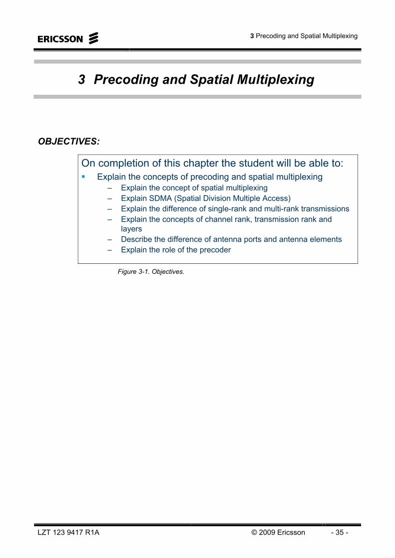
On completion of this chapter the student will be able to:Explain the concepts of precoding and spatial multiplexing
– Explain the concept of spatial multiplexing– Explain SDMA (Spatial Division Multiple Access)– Explain the difference of single-rank and multi-rank transmissions– Explain the concepts of channel rank, transmission rank and
layers– Describe the difference of antenna ports and antenna elements– Explain the role of the precoder
Figure 3-1. Objectives.

MIMO in WCDMA and LTE
- 36 - © Ericsson 2009 LZT 123 9417 R1A
Intentionally Blank
3 Precoding and Spatial Multiplexing
LZT 123 9417 R1A © 2009 Ericsson - 37 -
PRECODING FOR SPATIAL MULTIPLEXING, TX DIVERSITY AND BEAMFORMING
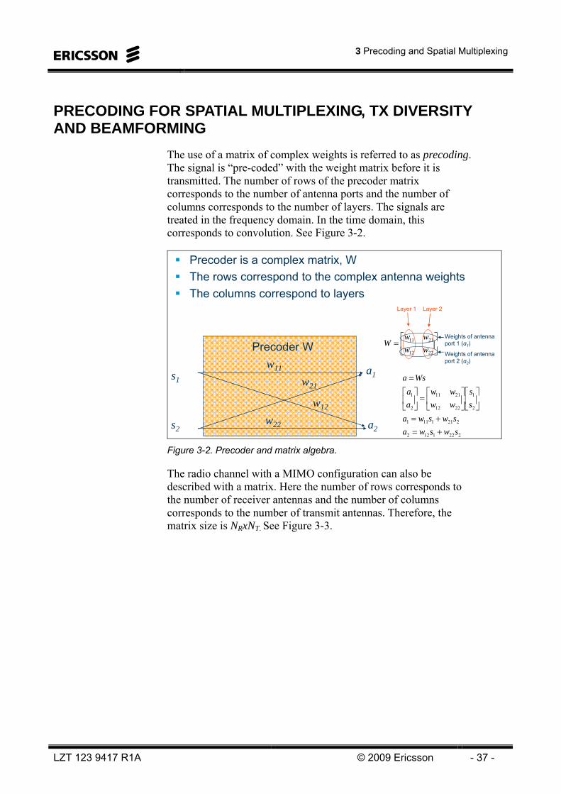
The use of a matrix of complex weights is referred to as precoding. The signal is “pre-coded” with the weight matrix before it is transmitted. The number of rows of the precoder matrix corresponds to the number of antenna ports and the number of columns corresponds to the number of layers. The signals are treated in the frequency domain. In the time domain, this corresponds to convolution. See Figure 3-2.
⎥⎦
⎤⎢⎣
⎡=
2212
2111
wwww
W
w11
w22
w21
w12
2221122
2211111
2
1
2212
2111
2
1
swswaswswa
ss
wwww
aa
Wsa
+=+=
⎥⎦
⎤⎢⎣
⎡⎥⎦
⎤⎢⎣
⎡=⎥
⎦
⎤⎢⎣
⎡
=s1
s2
a1
a2
Precoder is a complex matrix, WThe rows correspond to the complex antenna weightsThe columns correspond to layers
Precoder W
Layer 1 Layer 2
Weights of antenna port 1 (ɑ1)
Weights of antenna port 2 (ɑ2)
Figure 3-2. Precoder and matrix algebra.
The radio channel with a MIMO configuration can also be described with a matrix. Here the number of rows corresponds to the number of receiver antennas and the number of columns corresponds to the number of transmit antennas. Therefore, the matrix size is NRxNT. See Figure 3-3.

MIMO in WCDMA and LTE
- 38 - © Ericsson 2009 LZT 123 9417 R1A
⎥⎦
⎤⎢⎣
⎡=
2221
1211
hhhh
H
hay =
h11
h22
h12
h21
h
2221212
2121111
2
1
2221
1211
2
1
ahahyahahy
aa
hhhh
yy
Hay
+=+=
⎥⎦
⎤⎢⎣
⎡⎥⎦
⎤⎢⎣
⎡=⎥
⎦
⎤⎢⎣
⎡
=
y: received signal, a: transmitted signal on antenna port, h: radio channel transfer function
a
a1
a2
y1
y2
With MIMO, the radio channel transfer function becomes a matrix, H
Radio channel H
Figure 3-3. Radio channel and matrix algebra.
The complete transfer function is equal to the product (in the frequency domain) of the information signal s and the precoder matrix and the channel matrix.
w11
w22
w21
w12
s1
s2
Precoder Wh11
h22
h12
h21
a1
a2
Radio channel HReceiver
y1
y2
⎥⎦
⎤⎢⎣
⎡⎥⎦
⎤⎢⎣
⎡⎥⎦
⎤⎢⎣
⎡==
2
1
2212
2111
2221
1211
ss
wwww
hhhh
HWsy
Figure 3-4. Matrix operations.
In the receiver, the radio channel is estimated and compensated for. This corresponds to an estimation of the inverted channel transfer function and an inversion of the precoder matrix. The inverted radio channel transfer function can be estimated with e.g. a MMSE (Minimum Mean Square Error) equalizer.

3 Precoding and Spatial Multiplexing
LZT 123 9417 R1A © 2009 Ericsson - 39 -
yHWs
IWWWsWyHW
WsyH
IHH
HWsHyH
HWsy
11
1
111
1
1
11
ˆ)(
ˆ
ˆ)ˆ(
ˆˆ
−−
−
−−−
−
−
−−
≈
=≈
≈
≈
=
=
Radio channel is estimated and inversed: Ĥ-1
Inverse precoder matrix applied at receiver: W-1
Figure 3-5. Channel estimation and antenna demapping at receiver side.
SPATIAL MULTIPLEXING
MIMO (Multiple Input Multiple Output) refer to the multiple antenna configuration or setup. In its simplest case we have two tx antennas and two rx antennas. This is referred to as 2x2 MIMO. In general terms, NTxNR means “number of transmitter antennas” (intputs to the radio channel) and “number of receiver antennas” (outputs from the radio channel).
Figure 3-6 shows an example of a choice of optimum precoder matrix for transmission rank 2 in case of perfectly cross-polarized antennas and an ideal radio channel.
22
11
1001
1001
sysy
syW
==
⇒⎥⎦
⎤⎢⎣
⎡=⇒⎥
⎦
⎤⎢⎣
⎡=
1
1
00
s1s2
y1
y2
Figure 3-6. Example of cross polarized spatial multiplexing with rank 2.
MIMO in WCDMA and LTE
- 40 - © Ericsson 2009 LZT 123 9417 R1A
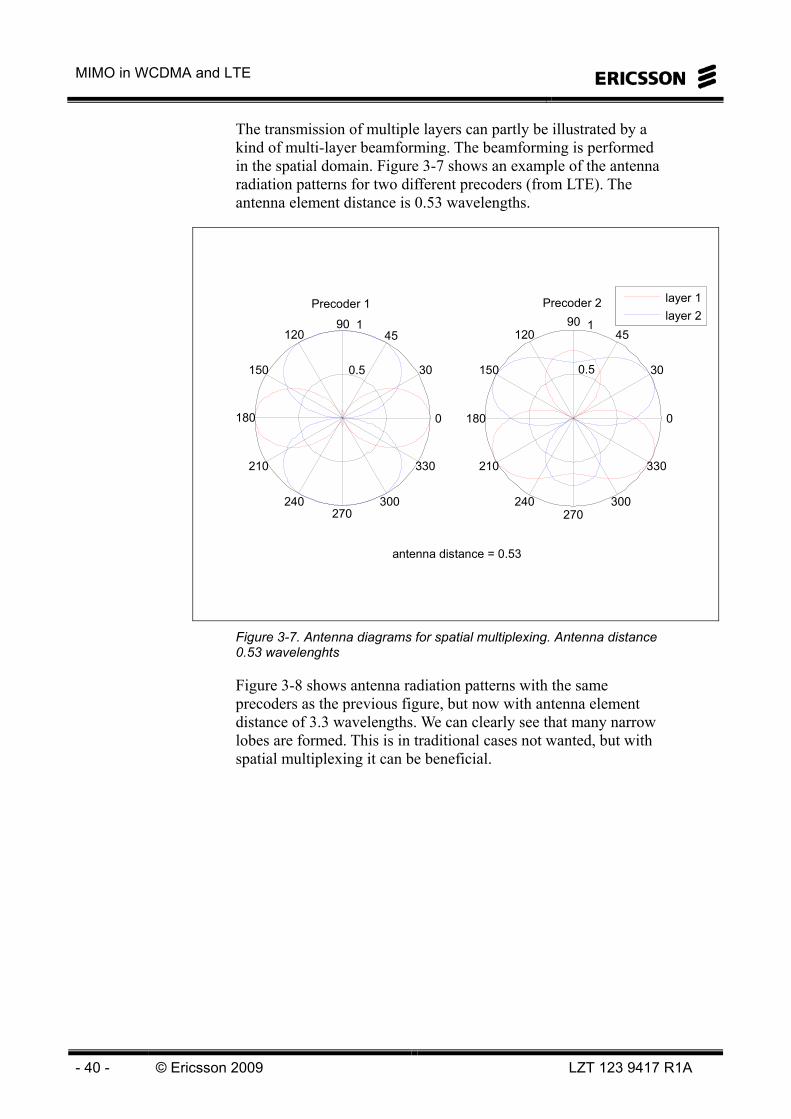
The transmission of multiple layers can partly be illustrated by a kind of multi-layer beamforming. The beamforming is performed in the spatial domain. Figure 3-7 shows an example of the antenna radiation patterns for two different precoders (from LTE). The antenna element distance is 0.53 wavelengths.
0.5 30
210
240270
120
300
150
330
180 0
Precoder 1
0.5 30
210
60
240
90
270
120
300
150
330
180 0
Precoder 2
antenna distance = 0.53
layer 1layer 2
9045 45
1 1
Figure 3-7. Antenna diagrams for spatial multiplexing. Antenna distance 0.53 wavelenghts
Figure 3-8 shows antenna radiation patterns with the same precoders as the previous figure, but now with antenna element distance of 3.3 wavelengths. We can clearly see that many narrow lobes are formed. This is in traditional cases not wanted, but with spatial multiplexing it can be beneficial.

3 Precoding and Spatial Multiplexing
LZT 123 9417 R1A © 2009 Ericsson - 41 -
0.5
1
30
210
60
240
90
270
120
300
150
330
180 0
Precoder 1
layer 1layer 2
0.5
1
30
210
60
240
90
270
120
300
150
330
180 0
Precoder 2
lambda = 3.3
layer 1layer 2
Figure 3-8. Antenna diagrams for spatial multiplexing. Antenna distance 3.3 wavelengths.
We can see in both previous figures that the antenna patterns are orthogonal in order to support independent layers.
Figure 3-9 shows a simple example of spatial multiplexing where different orthogonal beams transmits and receives two different layers.
0.2
0.4
0.6
0.8
1
30
210
60
240
90
270
120
300
150
330
180 0
0.2
0.4
0.6
0.8
1
30
210
60
240
90
270
120
300
150
330
180 0
Precoder 1
Precoder 1
RBS
Layer 1
Layer 2
Figure 3-9. Example of spatial multiplexing (SU-MIMO)

MIMO in WCDMA and LTE
- 42 - © Ericsson 2009 LZT 123 9417 R1A
The same principle is illustrated in Figure 3-10 and Figure 3-11, where we can see how two different precoders give rise to different antenna patterns that exploit the multi path propagation geometry in two different ways as the UE moves. This is an example of SDM (Spatial Division Multiplexing) and is in LTE referred to as Single-User MIMO (SU-MIMO)
RBS
Layer 1
Layer 2
⎥⎦
⎤⎢⎣
⎡−
=11
11W
Layer 2
Figure 3-10. Example of spatial multiplexing – DL SU-MIMO (SDM).
RBS
Layer 1
Layer 2
⎥⎦
⎤⎢⎣
⎡−
=jj
W11
Layer 2
Figure 3-11. Example of spatial multiplexing – DL SU-MIMO (SDM).

3 Precoding and Spatial Multiplexing
LZT 123 9417 R1A © 2009 Ericsson - 43 -
Figure 3-12 shows how spatial multiplexing can be used in order to separate different users. This is an example of SDMA (Spatial Division Multiple Access) and is in LTE referred to as Multi-User MIMO (MU-MIMO).
RBS
Layer 1Layer 2
⎥⎦
⎤⎢⎣
⎡−
=jj
W11
Layer 2
Figure 3-12. Example of spatial multiplexing - UL MU-MIMO (SDMA).
The spatial domain includes however more than the angular information that is illustrated in Figure 3-7 to Figure 3-12. It includes polarization and phase information. All these properties contribute to the spatial characteristics of the radio channel.
This can be illustrated with vectors. The spatial multiplexing is performed in the “vector space”, where the vectors include polarization and carrier phase information.
A UE reception may for instance be in a fading peak for one layer and one weight vector in the precoder matrix but in a fading dip for another layer with the same weight vector. The second layer may be in a fading peak for the second weight vector in the precoder matrix.
So, when MU-MIMO is used, the system will try to find multiple UEs (UE antenna ports) that are orthogonal (or at least sufficiently well separated) in the ”vector space” in either one or a combination of the following dimensions: • azimuth angle (horizontal antenna diagram)
• polarization
• fading (carrier wave phase)

MIMO in WCDMA and LTE
- 44 - © Ericsson 2009 LZT 123 9417 R1A
The UE signals will be separated in the receiver by applying the precoder on the receiver antenna ports.
Performed in the ”vector space”The vector space includes:
– Polarization– Antenna radiation pattern– Fading geometry
Figure 3-13. Spatial multiplexing.
When SU-MIMO is used, the system will try to find a precoder matrix that gives orthogonal (or at least sufficiently well separated) streams in the “vector space” after the receiver has performed its antenna demapping (applying the receiver precoder on its receiver antenna ports).

4 MIMO in WCDMA
LZT 123 9417 R1A © 2009 Ericsson - 45 -
4 MIMO in WCDMA
OBJECTIVES:
On completion of this chapter the student will be able to:Describe MIMO in WCDMA
– Explain Tx diversity in WCDMA– Explain spatial multiplexing in WCDMA– Describe the UE feedback (PCI)– Describe the configuration of MIMO in WCDMA
Figure 4-1. Objectives.

MIMO in WCDMA and LTE
- 46 - © Ericsson 2009 LZT 123 9417 R1A
Intentionally Blank

4 MIMO in WCDMA
LZT 123 9417 R1A © 2009 Ericsson - 47 -
MIMO IN WCDMA WCDMA RAN P7FP supports precoder-based 2x2 SU-MIMO as an optional feature. This feature allows for transmission of one or two data streams of HS-DSCH from 2 antenna arrays and reception on 2 antenna arrays in the downlink. Existing dual polarized antennas can be reused. 2x2 MIMO provides bit rates up to 28 Mbps (twice as much as without MIMO) and it also delivers an improved spectral efficiency and capacity.
Uplink
20-40 Mbps
12 Mbps
5.8 Mbps
1.4 Mbps
0.384 Mbps
2 ms TTI
16QAM
Downlink
3.6 Mbps
14 Mbps
21 Mbps 28 Mbps
42 Mbps
80-160 Mbps
15 codes
2x2 MIMO64QAM
Both
Multi Carrier4x4 MIMOHigher ModulationCombinations
Higher Speed, Lower cost per GByte
Multi Carrier
Figure 4-2. HSPA speed evolution.
Other channels, such as common channels, non-MIMO channels and Primary and Secondary SCH may use Tx Diversity. P&S-SCH uses TSTD (Time Switched Transmit Diversity), while the common channels, non-MIMO channels use STTD (Space Time Transmit Diversity).

MIMO in WCDMA and LTE
- 48 - © Ericsson 2009 LZT 123 9417 R1A
Precoder based 2x2 MIMO tx for HS-DSCHP-SCH and S-SCH use TSTD (Time Switched Transmit Diversity)Other channels use STTD (Space Time Transmit Diversity)Switching between dual and single stream MIMO per TTIPrecoding Control Info (PCI) is fed back from UE
– RBS may override PCI
Single stream MIMO similar to Tx diversity– Single stream MIMO precoder updated per TTI– Tx diversity weight updated per slot
Figure 4-3. MIMO in WCDMA.
However, the CL Tx Diversity cannot be used together with the fractional DPCH, so it is not used in Ericsson products.
Switching between MIMO and Tx Diversity for the HS-DSCH requires RRC signaling, while switching between dual and single stream MIMO can be done per TTI without RRC signaling.
28 Mbps
14 Mbps
Path loss / Distance from RBS
Higher speed, Longer range or Deeper indoor coverage
RXRXTXTX
Today
RXRXTXTX
Today
RXRXTXTX
Today
RXRXTXTX
TxDivTxDiv for legacy terminalsImproves speed at cell edgeRXRXTXTX
TxDiv
RXRXTXTX
TxDivTxDiv for legacy terminalsImproves speed at cell edge
MIMO for new terminalsMIMO Improves speed & capacityRXRXTXTX
MIMO
MIMO for new terminalsMIMO Improves speed & capacityRXRXTXTX
MIMO
RXRXTXTX
MIMO
Figure 4-4. MIMO and tx diversity.
With MIMO, two parallel data streams can be transmitted to one UE on the same set of HS-PDSCH codes, instead of one stream only as is the case with Rel-6 HS-PDSCH. This means that the peak bit rate for HS-DSCH can be doubled.

4 MIMO in WCDMA
LZT 123 9417 R1A © 2009 Ericsson - 49 -
Transmission of two parallel data streams (two parallel transport blocks) is denoted dual-stream transmission, while transmission of one stream only is denoted single-stream transmission. Single-stream transmission is quite similar to TX diversity with closed loop mode 1, but with the difference that the antenna weighting is updated once per TTI instead of once per slot for the TX diversity case.
The weighting of the streams and distribution over the two antennas is called precoding, and ensures that the HS-PDSCH power on the two antennas is the same, independent on if single-stream or dual-stream transmission is made.
The choice of precoder is based on feedback from the UE. This feedback includes CQI (Channel Quality Indicator) and PCI (Precoding Control Info). The PCI indicates the best precoding matrix (out of four possible matrices) as estimated by the UE from pilot measurements.
The P-CPICH is transmitted on antenna branch 1. An altered version of P-CPICH is transmitted on antenna branch 2. See Figure 4-5.
Turboencoder
w11
P-CPICH1DPCH, CCH ...
ModulationSpreadingScrambling w12
P-CPICH2 or S-CPICHDPCH, CCH ...
4/7,4/5,4/3,4/,ee11
21
jj2212
2111 ππππφφφ ∈⎥⎦
⎤⎢⎣
⎡−
=⎥⎦
⎤⎢⎣
⎡wwww
Calcprecoding
matrix
w11w12w21w22
Precoding control info (PCI) from UE
Single- / dual-stream CQIfeedback from UECQI
The PCI indicates the UE’s preferred value of w12, other three weights then known
022
21*
12
11 ≡⎥⎦
⎤⎢⎣
⎡⎥⎦
⎤⎢⎣
⎡ww
ww
(the two streams are orthogonal)
ModulationSpreadingScrambling
w21
w22
Turboencoder
HARQScheduler
&
TFRCselection
HARQ
Precoder W
Figure 4-5. Precoding in WCDMA.
The P-CPICH transmission on the two antenna branches enables the UE to estimate the spatial properties of the radio channel. The UE will select the pre-coder matrix that is estimated to give the best possible throughput and report it to the base-station in a PCI (Pre-coder Control Indicator) on HS-DPCCH.
The RBS may override the recommended PCI.

MIMO in WCDMA and LTE
- 50 - © Ericsson 2009 LZT 123 9417 R1A
If the radio channel happens not to support dual stream transmissions, the UE will report a PCI indicating that Single Stream MIMO should be used.
Single Stream MIMO is similar to Closed Loop Tx Diversity, but with the difference that in CL Tx Div, the chosen PCI is not echoed back to the UE and that the Tx Diversity is updated per slot (667μs) while Single Stream MIMO is updated per TTI (2ms).
In order to use MIMO, both TX diversity and support of Enhanced layer 2 are required. Also, the UEs need to be MIMO capable and the RBS must have one power amplifier per antenna branch.
MIMO is an optional feature both for RAN and UE in 3GPP Rel-7. Only UEs belonging to HS-DSCH UE categories 15, 16, 17, 18, 19 and 20 support this feature. This feature gives higher DL speeds of up to 28 Mbps for RABs using Enhanced uplink in uplink and HSDPA in downlink.
MIMO and 64QAM42.215Category 20
MIMO and 64QAM35.315Category 19
MIMO or 64QAM28 or 21.115Category 18
MIMO or 64QAM23.4 or 17.615Category 17
MIMO2815Category 16
MIMO23.415Category 15
64QAM21.115Category 14
64QAM17.615Category 13
QPSK1.85Category 12
QPSK0.95Category 11
16QAM14.015Category 10
16QAM10.215Category 9
16QAM7.310Category 8
16QAM7.310Category 7
16 QAM3.65Category 6
16QAM3.65Category 5
16QAM1.85Category 4
16QAM1.85Category 3
16QAM1.25Category 2
16QAM1.25Category 1
ModulationMIMO
L1 peak ratesMaximum codes
HS-DSCH category
Figure 4-6. HSPA terminal categories.
In P7FP, 64-QAM cannot be used simultaneous with MIMO.
To reach the highest bit rates SPB3 HW is required in the RNC. Also, core network support is required for the higher bitrates.

4 MIMO in WCDMA
LZT 123 9417 R1A © 2009 Ericsson - 51 -
MIMO is supported over Iur. The capability of MIMO for the neighbour inter-RNS cells has to be configured in the MO ExternalUtranCell (parameter transmissionScheme). Concerning cells that belong to the UTRAN network, the capability is transferred from the MO UtranCell by means of the OSS-RC. Cells that belong to an external UTRAN network have to be configured manually by the operator.
RANAP Rel-7 is needed if QoS parameters GBR and MBR are set to values above 16 Mbps.
If MIMO is configured for the cell in the RNC but not in the RBS the cell setup will fail and the alarm UtranCell_NbapMessageFailure with a new alarm cause MIMO not available will be issued.
The following new performance management counters are defined for MIMO:
• pmReportedCqiMimoSs: Counter for received single-stream CQI reports on MIMO-activated connections
• pmReportedCqiMimoDs1: Counter for received primary-stream CQI reports (when dual-stream CQI is received) on MIMO-activated connections
• pmReportedCqiMimoDs1: Counter for received secondary-stream CQI reports (when dual-stream CQI is received) on MIMO-activated connections
The existing performance management counter pmUsedCqi is not easily extended to cover also MIMO because of the changed CQI reporting tables with multiple SIR step sizes. This counter is discontinued for MIMO users, i.e. the counter only counts used CQIs if the HS-DSCH is MIMO-deactivated.
Tx Diversity
Transmit Diversity is a technique that improves the downlink radio link performance in terms of capacity and cell edge bit rate.
Different types of transmit diversity can be used at the base station to improve the capacity. A diversity gain is achieved in the UE by coding the information bits, which are transmitted, differently.
The TX diversity is applied to all channels in the cell if the feature is enabled.

MIMO in WCDMA and LTE
- 52 - © Ericsson 2009 LZT 123 9417 R1A
Open-loop transmit diversity
TX Diversity is an optional feature which includes Time-Switched Transmit Diversity (TSTD) and Space-Time Transmit Diversity (STTD), i.e. open loop mode.
Note that all UEs must support both STTD and TSTD but it is optional in the RBS.
TSTD is used only on the synchronization channels. The SCH with primary and secondary code are alternated between antenna 1 and 2 for each time slot in the WCDMA frame as shown in Figure 4-7.
aPSC
aSSCi
aPSC
aSSCi
aPSC
aSSCi
aPSC
aSSCi
aPSC
aSSCi
Antenna 1
Antenna 2
Slot #0 Slot #1 Slot #2 Slot #3 Slot #14
aPSC
aSSCi
aPSC
aSSCi
aPSC
aSSCi
aPSC
aSSCi
aPSC
aSSCi
Antenna 1
Antenna 2
Slot #0 Slot #1 Slot #2 Slot #3 Slot #14
Note: TSTD must be supported by the UE, but are optional in BS
3GPP TS 25.211 ¶ 5.33GPP TS 25.211 ¶ 5.3
a = 1 P-CCPCH is STTD encodeda = -1 P-CCPCH is not STTD encoded
TSTD (Time-Switched Transmit Diversity); SCH Only
Figure 4-7: Transmit Diversity – TSTD
When the UE monitors the synchronization codes it will be able to determine if P-CCPCH, which carries the transport channel BCH, is STTD encoded. The synchronization codes are modulated with a = 1 if the P-CCPCH is STTD encoded and a = -1 if P-CCPCH is not STTD encoded.
STTD is used on all other DL channels. The data symbols are transmitted again on the second antenna with the phase reversed. The pattern depends on which modulation scheme that is used, as shown in Figure 4-8.

4 MIMO in WCDMA
LZT 123 9417 R1A © 2009 Ericsson - 53 -
b0 b1 b2 b3
b0 b1 b2 b3
-b2 b3 b0 -b1
Antenna 1
Antenna 2
Symbolsb0 b1 b2 b3
b0 b1 b2 b3
-b2 b3 b0 -b1
Antenna 1
Antenna 2
Symbols
STTD (Space-Time Transmit Diversity); All Other DL Channels
Note: STTD must be supported by the UE, but are optional in BS
3GPP TS 25.211 ¶ 5.33GPP TS 25.211 ¶ 5.3
b0 b1 b2 b3
Symbolsb4 b5 b6 b7
b0 b1 b2 b3
-b4 b5 b6 b7 b0 -b1 b2 b3
b4 b5 b6 b7 Antenna 1
Antenna 2
b0 b1 b2 b3
Symbolsb4 b5 b6 b7
b0 b1 b2 b3
-b4 b5 b6 b7 b0 -b1 b2 b3
b4 b5 b6 b7 Antenna 1
Antenna 2
Antenna 1
Antenna 2
b0 b1 b2 b3
Symbolsb4 b5 b6 b7 b8 b9 b10 b11
b0 b1 b2 b3 b4 b5 b6 b7 b8 b9 b10 b11
-b6 b7 b8 b9 b10 b11 b0 -b1 b2 b3 b4 b5
Antenna 1
Antenna 2
Antenna 1
Antenna 2
b0 b1 b2 b3
Symbolsb4 b5 b6 b7 b8 b9 b10 b11
b0 b1 b2 b3 b4 b5 b6 b7 b8 b9 b10 b11
-b6 b7 b8 b9 b10 b11 b0 -b1 b2 b3 b4 b5
Antenna 1
Antenna 2
QPSK 16QAM
64QAM
Figure 4-8. Transmit Diversity – STTD
Since STTD is applied on all DL channels, except SCH, some of the channels will differ from what is stated above. All DL channels will be coded as in Figure 4-8 with some exceptions, according to 3GPP technical specification 25.211.
CPICH will still have zeroes as input on the first antenna. But the second antenna has a bit pattern which start with 00 in the first slot followed by 1111 and 0000 alternated for the rest of the time slots in one frame, as shown in Figure 4-9.
The input to CPICH differs between the antennas if STTD is used
0 0 0 0 0 0 0 0 0 0 0 0 0 0 0 0 0 0 0 00 0 0 0 0 0 0 0 0 0 0 0 0 0 0 0 0 0 0 0
0 0 1 1 1 1 0 0 0 0 1 1 1 1 0 0 0 0 1 10 0 1 1 1 1 0 0 0 0 1 1 1 1 0 0 0 0 1 1 1 1 0 0 0 0 1 1 11 1 0 0 0 0 1 1 1 ......
1 1 1 0 0 0 0 1 11 1 1 0 0 0 0 1 1
...
...0 0 0 0 0 0 0 0 00 0 0 0 0 0 0 0 00 0 0 0 0 0 0 0 00 0 0 0 0 0 0 0 0
...
...
...
...Antenna 1
Antenna 2
Slot #0Slot #14 Slot #1
Frame #n-1 Frame #n
3GPP TS 25.211 ¶ 5.33GPP TS 25.211 ¶ 5.3
Figure 4-9. CPICH Modulation Pattern (STTD)

MIMO in WCDMA and LTE
- 54 - © Ericsson 2009 LZT 123 9417 R1A
The encoding on the data bits (BCH) in P-CCPCH also differs. P-CCPCH is encoded as described in Figure 4-8. However, the last two data bits in even numbered slots are STTD encoded together with the first two data bits in the following slot, since BCH consists of 18 bits in each slot and QPSK is used. This applies for all time slots except the last two bits in the last time slot in each frame. These bits are transmitted by both antennas with equal power, hence not STTD encoded as shown in Figure 4-10.
STTD encoded
Transmitted on both antennas with equal power
BCHBroadcast Channel (18 bits)
BCHBroadcast Channel (18 bits)
BCHBroadcast Channel (18 bits)
STTD encoded STTD encoded
Slot #14 Slot #0 Slot #1
......
STTD encoded
Transmitted on both antennas with equal power
BCHBroadcast Channel (18 bits)
BCHBroadcast Channel (18 bits)
BCHBroadcast Channel (18 bits)
STTD encoded STTD encoded
Slot #14 Slot #0 Slot #1
......
3GPP TS 25.211 ¶ 5.33GPP TS 25.211 ¶ 5.3
Figure 4-10. P-CCPCH Modulation Pattern (STTD)
TX diversity will be used if the feature is activated in the cell with parameter transmissionScheme. This parameter is specified per UtranCell and per ExternalUtranCell, since TX diversity is supported over Iur. If this precondition is not fulfilled the RAB will be set up without TX Diversity.
The RBS has to be equipped with two TX branches. The following base stations support TX diversity:
• RBS R3b Macro: RBS 3106, RBS 3206 • RBS R1 / RBS R2 Macro: RBS 3101, RBS 3202 • RBS R3b Main-Remote: RBS 3412, RBS 3518, RBS 3418 • RBS 6000: RBS 6201, RBS 6102
The number of TX branches per sector is configurable by the operator controlled parameter numberOfTxBranches.

4 MIMO in WCDMA
LZT 123 9417 R1A © 2009 Ericsson - 55 -
Parameters for MIMO and Tx diversity
Parameter Name Default Value Value Range ResolutionUnit transmissionScheme SINGLE_ANTENNA SINGLE_ANTENNA = 0
TX_DIVERSITY = 1 TX_DIVERSITY_AND_MIMO = 2
- -
numberOfTxBranches 1 1..2 1 # of TX Branches
featureStateMIMO DECTIVATED DEACTIVATED/ACTIVATED - -
transmissionScheme: Indicates if TX Diversity and MIMO are enabled or not in the RNC. Exists in both UtranCell and ExternalUtranCell.
featureStateMIMO: Indicates if MIMO is enabled or not in the RBS.
MIMO will be used if the feature is activated in the cell in RNC transmissionScheme (this parameter is specified per UtranCell and per ExternalUtranCell), if the feature is activated in the cell in RBS featureStateMIMO, if the UE supports MIMO and if the target RAB supports MIMO. If any of the preconditions are not fulfilled the RAB will be set up without MIMO.
TX Diversity and Enhanced L2 are prerequisites for MIMO, if TX Diversity and Enhanced L2 are not enabled then MIMO cannot be enabled. MIMO is not compatible with 64QAM, i.e. they cannot both be used in the same connection. MIMO will be selected before 64QAM if the conditions for both are met.

MIMO in WCDMA and LTE
- 56 - © Ericsson 2009 LZT 123 9417 R1A
Intentionally Blank

5 MIMO in LTE
LZT 123 9417 R1A © 2009 Ericsson - 57 -
5 MIMO in LTE
OBJECTIVES:
On completion of this chapter the student will be able to:Describe MIMO in LTE
– Explain Tx diversity in LTE– Describe SU-MIMO and MU-MIMO– Explain spatial multiplexing in LTE– Describe the UE feedback (CSI, PMI, RI and CQI) in LTE– Describe open loop spatial multiplexing in LTE– Describe closed loop spatial multiplexing in LTE– Describe the configuration of MIMO in LTE
Figure 5-1. Objectives.

MIMO in WCDMA and LTE
- 58 - © Ericsson 2009 LZT 123 9417 R1A
Intentionally Blank

5 MIMO in LTE
LZT 123 9417 R1A © 2009 Ericsson - 59 -
MIMO IN LTE The LTE specifications support the use of multiple antennas at both transmitter (tx) and receiver (rx). MIMO (Multiple Input Multiple Output) uses this antenna configuration.
The LTE specifications support up to four antennas at the tx side and up to four antennas at the rx side (here referred to as 4x4 MIMO configuration).
In the first release of LTE it is likely that the UE only has one tx antenna, even if it uses two rx antennas. This leads to that so called Single User MIMO (SU-MIMO) will be supported only in DL (and maximum 2x2 configuration).
Single user MIMO (SU-MIMO)– Precoded spatial multiplexing with rank adaption– Used in DL
Multi user MIMO (MU-MIMO)– Tailored for multiple UEs per RB– Max one layer per UE– Used in UL
Transmit diversity– Block code based– Used in DL
Figure 5-2. LTE MIMO schemes.
SU-MIMO increases the data rate for a single user by creating several layers for that user. In UL multi user MIMO can be applied. This means that the base-station uses MU-MIMO to separate different UE transmissions spatially. This leads to that several UEs can be scheduled in the same resource block simultaneously (same frequency, same time). This increases the capacity in the cell.
There are seven different transmission modes in LTE, as defined by 3GPP TS 36.213. Switching between the modes is done by RRC signaling. • Mode 1 (”Single antenna port, port 1”)
o One antenna
o Can be used for classical beamforming without precoding feedback
• Mode 2 (”Transmit Diversity”)
o SFBC (Alamouti)
o 2 or 4 tx antennas

MIMO in WCDMA and LTE
- 60 - © Ericsson 2009 LZT 123 9417 R1A
• Mode 3 (”Open loop spatial multiplexing”)
o 2 or 4 tx antennas
o CQI and RI feedback
o Tx schemes:
Tx diversity
Large delay CDD
• Mode 4 (”Closed Loop spatial multiplexing”)
o 2 or 4 tx antennas
o CQI, PMI and RI feedback
o Tx schemes:
Tx diversity
CL SM
• Mode 5 (”Multi User MIMO”)
o Two UEs can be scheduled in the same RB
o Tx schemes:
Tx diversity
MU-MIMO
• Mode 6 (”Closed loop spatial multiplexing, single layer”)
o As mode 4, but with RI hardcoded to 1
o Tx schemes:
Tx diversity
CL SM
• Mode 7 (”Single antenna port, port 5”)
o Can be used for classical beamforming without feedback.
The transmission modes defined by 3GPP is shown in Figure 5-3. The names in brackets are not the formal names.

5 MIMO in LTE
LZT 123 9417 R1A © 2009 Ericsson - 61 -
Mode 1 (”Single antenna port, port 1”)Mode 2 (”Transmit Diversity”)Mode 3 (”Open loop spatial multiplexing”Mode 4 (”Closed Loop spatial multiplexing”)Mode 5 (”Multi User MIMO”)Mode 6 (”Closed loop spatial multiplexing, single layer”)Mode 7 (”Single antenna port, port 5”)
Figure 5-3. 3GPP LTE DL transmission modes.
Every transmission mode can use one or more transmission schemes. Typically, the transmission mode is set-up at session establishment and not changed during the session, while the transmission scheme is dynamically decided every TTI.
High SINRs needed– Service area close to cell center
Less likely that cell edge UEs use multiple layers- go for beamforming or diversity instead
Service area grows if surrounding cells have low load– Multiple layers on or near the cell edge not uncommon
MU-MIMO SU-MIMO
Figure 5-4. Spatial multiplexing operation.
Multiple layers means that the time- and frequency resources (Resource Blocks) can be reused in the different layers up to a number of times corresponding to the channel rank. This means that the same resource allocation is made on all transmitted layers.

MIMO in WCDMA and LTE
- 62 - © Ericsson 2009 LZT 123 9417 R1A
OFDM works particularly well with MIMO – MIMO becomes difficult when there is time dispersion– OFDM sub-carriers are flat fading (no time dispersion)
3GPP supports one, two, or four transmit Antenna PortsMultiple antenna ports Multiple time-frequency grids Each antenna port defined by an associated Reference Signal
Antenna port #1Antenna port #2Antenna port #3Antenna port #4
Single-antenna transmisson
Multi-antenna transmisson
Figure 5-5. Multi-antenna transmission.
In MU-MIMO, the different UEs that are spatially multiplexed are allocated the same resource blocks, but spatially separated by the antenna arrangement and associated processing. This means that each UE does not experience a data rate multiplication as with SU-MIMO. Instead the cell benefits from the reuse of the resources.
High load at least in cell of interest in order to find UEs for co-scheduling
– Grouping UEs need careful scheduler design and soundingHigh SINRs needed
– MU-MIMO service area close to cell centerLess likely that cell edge UEs use MU-MIMO
Similar to single user MIMO (SU-MIMO) except the transmissions now come from different UEs
– Uplink SU-MIMO not yet supported in LTE
Figure 5-6. MU-MIMO operation.
LTE uses precoder based MIMO operation. A precoder, which is a complex matrix of size equal to the number of layers times the number of transmit antennas, is used to form the “beams” for the different layers separately.

5 MIMO in LTE
LZT 123 9417 R1A © 2009 Ericsson - 63 -
Spatial Multiplexing w. Pre-coding based Beam-forming– Multiple parallel data streams Higher data rates– One or two code words– Number of layers ≤ Number of antenna ports– Pre-coding weights based on UE feedback (beam-forming)
Transmit Diversity (”open-loop”)– Transmission of same information from multiple antenna ports
Diversity– One code word
Layermapping Precoding
Up to four layers
RE mappingUp to four
”Antenna Ports”
RE mapping
One or two code words
Multi-antenna processing
Figure 5-7. LTE Multi-antenna transmission.
When spatial multiplexing is used, maximum two codewords (transport blocks) per TTI will be used. When no spatial multiplexing is used, only one codeword per TTI will be used.
Maximum of two code wordsMapping to up to four layers
– Number of layers depends on channel ”rank”– Dynamically adjusted based on UE reports
One layer(No MIMO)
Two layers Three layers Four layers
One code word Two code words Two code words Two code words
Transport format (modulation scheme and code rate)may differ between the code wordsSame number of symbols on each layer
Layermapping
Up to four layers
Figure 5-8. DL spatial multiplexing - layer mapping.

MIMO in WCDMA and LTE
- 64 - © Ericsson 2009 LZT 123 9417 R1A
Given the minimum number of transmit or receive antennas, the transmission rank can at maximum be equal to that minimum number. For example, if four transmit antennas and two receive antennas are used, then the transmission rank can one or two. If the transmission rank is lower than the channel rank (i.e. there are more antennas than layers), then the remaining antenna ports can be used for beamforming at the same time as the spatial multiplexing.
The number of useful layers is here denoted r, and the maximum number of layers rmax.
One symbol from each of NL layers linearly mapped to NA antenna ports
UE reports recommended precoder matrix W (including channel rank)– Set of available precoder matrices = The precoder ”code book”
Used precoder matrix signaled by network– Network does not need to follow UE recommendation
One layer ”Closed-loop” TX diversity = ”Beam forming”
x
PrecodingW
yxWy ⋅=
4 antenna portsLayer 1
Layer 2
Layer 3
Example: NL = 3, NA = 4
Figure 5-9. DL spatial multiplexing.
In the DL, the UE estimates the spatial properties of the radio channel by measuring the DL reference symbols from the different antenna ports. This estimation is used to give feedback to the eNodeB so that the eNodeB can allocate an appropriate amount of resources make an optimal antenna mapping.
The feedback is the CQI (Channel Quality Index), the PMI (Precoder Matrix Indicator) and the RI (Rank Indicator). The CQI reflects the channel quality and is used whether or not spatial multiplexing is used. The RI indicates the number of useful layers, as estimated by the UE and the PMI indicates the precoder matrix that the UE considers as the best (gives the highest estimated SINR).

5 MIMO in LTE
LZT 123 9417 R1A © 2009 Ericsson - 65 -
UE feeds back channel state information (CSI) to assist link adaptation and scheduling
– RI: Rank IndicatorRecommended transmission rank
– CQI(s): Channel Quality Indicator(s)Recommended transport format giving 10% BLERFrequency-selective reporting possible
– For closed-loop spatial multiplexingPMI(s): Precoder Matrix Indicator(s)Frequency-selective reporting possible
– CSI sensitive to feedback delay
S/P Rec
Coding & Modulation
Coding & Modulation
CSI Feedback
CW2layer & Precoder
Figure 5-10. UE feedback of CSI.
Codeword to layer mapping (CW2layer)– 2 Tx at NodeB: max 2 layers– 4 Tx at NodeB: max 4 layers
Note: Always max two codewords (transport blocks)Precoder Wf selected from finite codebook(except possibly in type II)
– UE recommends precoder to be used at NodeB side– Finest frequency granularity: one precoder per 5 RB– Single Tx rank r reported per subframe
May be combined with cyclic delay diversity (CDD)
yf
Codeword 1
Codeword 2
Mod
Mod
CW2layer Wf
IDFT
IDFT
sf
DFT
DFT
PrecoderLayers
Figure 5-11. Precoding with spatial multiplexing.
The UE will measure the different reference signals, which are transmitted separately on the different antenna ports in DL, and estimate the optimal precoder weights. The UE will choose a precoder matrix from a finite codebook, that consists of a number of precoder matrixes. Only the index of the chosen precoder matrix (Precoder Matrix Index – PMI) and Rank Indicator (RI) will be signaled to the eNB, together with the CQI.
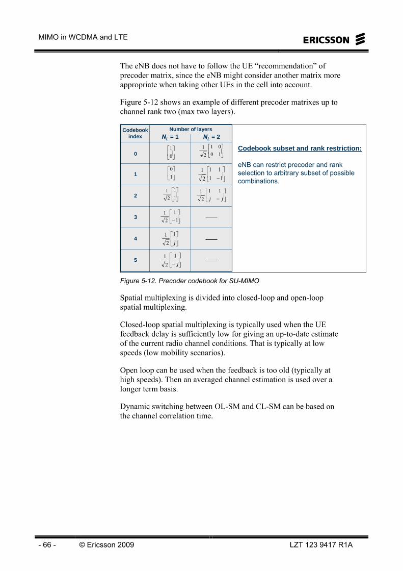
MIMO in WCDMA and LTE
- 66 - © Ericsson 2009 LZT 123 9417 R1A
The eNB does not have to follow the UE “recommendation” of precoder matrix, since the eNB might consider another matrix more appropriate when taking other UEs in the cell into account.
Figure 5-12 shows an example of different precoder matrixes up to channel rank two (max two layers).
⎥⎦
⎤⎢⎣
⎡1001
21
⎥⎦
⎤⎢⎣
⎡10
⎥⎦
⎤⎢⎣
⎡−11
21
⎥⎦
⎤⎢⎣
⎡11
21
⎥⎦
⎤⎢⎣
⎡01
⎥⎦
⎤⎢⎣
⎡−1111
21
⎥⎦
⎤⎢⎣
⎡− j1
21
⎥⎦
⎤⎢⎣
⎡j1
21
⎥⎦
⎤⎢⎣
⎡− jj11
21
5
4
3
2
1
0
NL = 2Codebook
indexNumber of layers
NL = 1
Codebook subset and rank restriction:
eNB can restrict precoder and rank selection to arbitrary subset of possible combinations.
Figure 5-12. Precoder codebook for SU-MIMO
Spatial multiplexing is divided into closed-loop and open-loop spatial multiplexing.
Closed-loop spatial multiplexing is typically used when the UE feedback delay is sufficiently low for giving an up-to-date estimate of the current radio channel conditions. That is typically at low speeds (low mobility scenarios).
Open loop can be used when the feedback is too old (typically at high speeds). Then an averaged channel estimation is used over a longer term basis.
Dynamic switching between OL-SM and CL-SM can be based on the channel correlation time.

5 MIMO in LTE
LZT 123 9417 R1A © 2009 Ericsson - 67 -
Closed-loop spatial multiplexing mode:– Precoder Wf focuses transmission in ”strong directions” towards
the UEWf selected from finite codebookTrack the channel in time as well as in frequency
– Targeting scenarios with accurate CSI at eNodeBTypically low mobility(unless highly spatially correlated channel)
Open-loop spatial multiplexing mode:– Transmit in ”all directions” by cycling through a sequence of four
different precoders Wf during the transmission of a singlesubframe
Transmission rank one utilizes transmit diversity– Targeting scenarios with inaccurate CSI at eNodeB
Typically high mobility
Go for diversity to achieve robustness!
Track instantanous channel to achieve array gain!
Figure 5-13. Closed and open loop spatial multiplexing.
The feedback from the UE to the eNodeB is called Channel State Information (CSI) and includes the CQI, PMI and RI. The CSI reporting can be made either periodically or a-periodically.
Periodic CSI on PUCCH– Similar to HSDPA– Narrow bit pipe → small payload size → rough report– Wideband CSI appropriate
Aperiodic dynamically requested CSI on PUSCH– Request CSI when needed!– Wide flexible bit pipe → large paylod size → detailed report– Frequency-selective CSI appropriate
Supports frequency domain schedulingArray gain in frequency-selective uncorrelatedchannels
Periodic CSI as baseline for more detailed aperiodic reports
Figure 5-14. Periodic and Aperiodic CSI.
The CQI and the PMI can be either a wide-band average over the whole system bandwidth or as frequency-selective (sub-band) reports.

MIMO in WCDMA and LTE
- 68 - © Ericsson 2009 LZT 123 9417 R1A
The CSI is reported on either PUCCH or PUSCH. There are many different formats that can be used for this reporting. Figure 5-15 illustrates the possible usage of the reporting modes for the different types of CQIs and PMIs.
Nine different CSI modes – 4 on PUCCH– 5 on PUSCH– Only a subset of modes possible for a certain transmission mode
RI: UE recommends single wideband rank
Wideband CQIFrequency- selective
CQI
Wideband PMI Frequency- selectivePMI
Wideband PMI
Frequency- selectivePMI
PUCCH 2-0 PUSCH 3-0, 2-0PUCCH 1-0
PUCCH 1-1 PUSCH 1-2
PUCCH 2-1 PUSCH 3-1
PUSCH 2-2
Figure 5-15. Reporting modes.
The UE estimates the CSI according to an algorithm summarized as an example in Figure 5-16.
Brute force search for best combination of RI and PMIIdeal algorithm:
– for each RI dofor each PMI do
- compute SINR per layer- SINRs → predicted throughput
– Select RI and PMI that gives highest predicted throughput over relevant reference period and bandwidth
– Given selected RI and PMI(s)Based on SINR(s) for transport block findhighest transport format with BLER ≤ 10% → CQI
Figure 5-16. UE calculation of CSI.
Different radio channel scenarios require different MIMO modes. Sometimes beamforming is most suitable, typically at bad SINRs close to cell edges, and sometimes spatial multiplexing is beneficial, typically closer to the basestation. Of course there are exceptions to this assumptions. Figure 5-17 summarizes the most likely usage of the different modes.
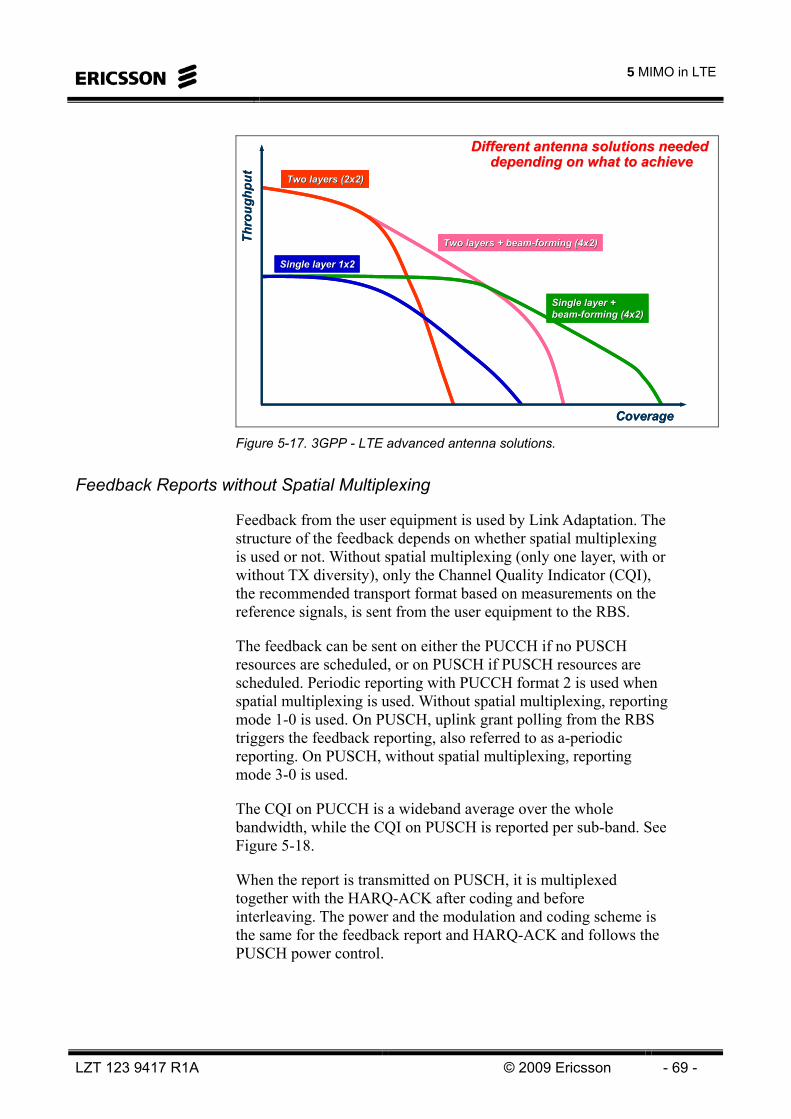
5 MIMO in LTE
LZT 123 9417 R1A © 2009 Ericsson - 69 -
Two layers + beamTwo layers + beam--forming (4x2)forming (4x2)Two layers + beamTwo layers + beam--forming (4x2)forming (4x2)
Two layers (2x2)Two layers (2x2)Two layers (2x2)Two layers (2x2)
Single layer + Single layer + beambeam--forming (4x2)forming (4x2)Single layer + Single layer + beambeam--forming (4x2)forming (4x2)
Single layer 1x2Single layer 1x2Single layer 1x2Single layer 1x2
Coverage
Thro
ughp
ut
Coverage
Thro
ughp
ut
Different antenna solutions needed Different antenna solutions needed depending on what to achievedepending on what to achieve
Figure 5-17. 3GPP - LTE advanced antenna solutions.
Feedback Reports without Spatial Multiplexing
Feedback from the user equipment is used by Link Adaptation. The structure of the feedback depends on whether spatial multiplexing is used or not. Without spatial multiplexing (only one layer, with or without TX diversity), only the Channel Quality Indicator (CQI), the recommended transport format based on measurements on the reference signals, is sent from the user equipment to the RBS.
The feedback can be sent on either the PUCCH if no PUSCH resources are scheduled, or on PUSCH if PUSCH resources are scheduled. Periodic reporting with PUCCH format 2 is used when spatial multiplexing is used. Without spatial multiplexing, reporting mode 1-0 is used. On PUSCH, uplink grant polling from the RBS triggers the feedback reporting, also referred to as a-periodic reporting. On PUSCH, without spatial multiplexing, reporting mode 3-0 is used.
The CQI on PUCCH is a wideband average over the whole bandwidth, while the CQI on PUSCH is reported per sub-band. See Figure 5-18.
When the report is transmitted on PUSCH, it is multiplexed together with the HARQ-ACK after coding and before interleaving. The power and the modulation and coding scheme is the same for the feedback report and HARQ-ACK and follows the PUSCH power control.

MIMO in WCDMA and LTE
- 70 - © Ericsson 2009 LZT 123 9417 R1A
When no CQI resources are configured on PUCCH for user equipment, or when there is downlink traffic, the link adaptation must schedule the feedback reports on PUSCH. The CQI reflects the recommended transport format of the modulation scheme and coding rate. The CQI is estimated by the user equipment from measurements on the downlink reference signal and Signal to Noise and Interference Ratio (SINR).
Feedback Reports with Spatial Multiplexing
With spatial multiplexing, a more extensive feedback report is needed. The structure depends on whether open or closed loop spatial multiplexing is used.
The feedback for closed loop consists of Channel Quality Indicator (CQI), Precoder Matrix Indicator (PMI), and Rank Indicator (RI). For the closed loop there are separate CQIs per layer. The CQI on PUCCH is a wideband report, while the CQI on PUSCH is reported per subband in case of open loop spatial multiplexing. Closed loop uses a wideband report on PUSCH.
The feedback for open loop uses only CQI and RI. The PUCCH report is periodically scheduled, with CQI and PMI on one rate and RI on another rate. For open loop, there is one CQI sent from the user equipment to the RBS.
The number of CQI resources per slot is configurable.
The periodicity of the reporting is common for all user equipment in the cell. On PUCCH the reporting mode for closed loop is 1-1 and for open loop 1-0. On PUSCH, the reporting mode is 1-2 for closed loop and 3-0 for open loop.
The PUSCH and PUCCH reporting modes and CQI and PMI feedback types are shown in Figure 5-18.
YESWide-band
Wide-band
1-1YESSub-band
Wide-band
1-2Closed Loop
YES-Wide-band
1-0YES-Sub-band
3-0Open Loop
-Wide-band
1-0--Sub-band
3-0No Spatial Mux/Tx Div
RIPMICQIReporting Mode
RIPMICQIReporting Mode
PUCCHPUSCH
YESWide-band
Wide-band
1-1YESSub-band
Wide-band
1-2Closed Loop
YES-Wide-band
1-0YES-Sub-band
3-0Open Loop
-Wide-band
1-0--Sub-band
3-0No Spatial Mux/Tx Div
RIPMICQIReporting Mode
RIPMICQIReporting Mode
PUCCHPUSCH
Figure 5-18. PUSCH and PUCCH Reporting Modes.

5 MIMO in LTE
LZT 123 9417 R1A © 2009 Ericsson - 71 -
The sub-band size is configured by higher layers, according to 3GPP TS 36.213.
With tx diversity, DCI (DL Control Information) format 1 is supported.
With spatial multiplexing, DCI format 2A is supported. This DCI format includes allocation of two transport blocks with different modulation and coding schemes (MCSes) as well as bitmap based resource allocation.
The Dual Antenna DL Performance Package feature is controlled by the parameter featureStateDualAntDlPerfPkg. The license will have a dependency towards MOM configuration of noOfTxAntennas.
The Dual antenna downlink performance package introduces two different multi antenna transmission schemes to the LTE RAN downlink; Transmit diversity (Transmission mode 2) and Open loop spatial multiplexing (transmission mode 3).
The Transmit diversity mode utilizes an Alamouti (space-frequency block code) scheme in the frequency domain to transmit one codeword on two antennas.
The transmit diversity scheme is always rank 1 and does not in itself enhance the data rates. Instead, the gain in using transmit diversity is that it provides a better received signal quality (SINR) at the UE side.
The Open loop spatial multiplexing mode supports both rank 1 and rank 2 transmissions. The rank 1 form of this scheme is equivalent to transmit diversity, as described above. The rank 2 form uses large delay cyclic diversity (CDD) to transmit two codewords on two antennas by using spatial multiplexing. If the right conditions are fulfilled, this enhances the data rates.
Open loop spatial multiplexing in LTE is an adaptive multi-antenna scheme that selects the scheme with the most suitable properties, to optimize the usage of the radio resource. For lower SINR, transmit diversity is the best suited multi-antenna scheme. For higher values of SINR, the UE benefits from using spatial multiplexing.

MIMO in WCDMA and LTE
- 72 - © Ericsson 2009 LZT 123 9417 R1A
To adaptively switch the rank of the transmission, as in the Open loop spatial multiplexing mode, channel state information is necessary at the transmitter side. In LTE, the UE estimates the signal quality and decides the most suitable rank for transmission. Information about signal quality and preferred rank is fed back in CQI reports and rank indicators (RI) to the base station. If the Transmit diversity mode is used, rank indicators are not transmitted since the rank is statically set to 1. Precoding matrix information (PMI) is not necessary for open loop spatial multiplexing since large delay CDD is used.
At connection to a cell, the UE is configured to provide channel state information with different contents and frequency, depending on the transmission mode.
If the transmission mode is set to “Transmit diversity”, the UE is requested to provide channel quality indicator (CQI) reports periodically on the physical uplink control channel (PUCCH). If the transmission mode is set to “Open loop spatial multiplexing”, the UE is, in addition to CQI, requested to periodically report rank indicators (RI) on PUCCH. The frequency and contents of the periodic CSI reporting is set via RRC messaging.
In addition to this, the UE may also send aperiodic CQI reports together with data on the physical uplink shared channel (PUSCH). These reports are requested by link adaptation and are configured to contain information on the channel quality.
Downlink scheduling and Link adaptation
For a UE that is selected for scheduling, the first step is to select a downlink control information (DCI) format. In case the transmission mode is set to “Open loop spatial multiplexing”, DCI format 2A is selected. If transmission mode is set to “Transmit diversity”, DCI format 1 is selected. DCI format 2A supports transmission on one or two codewords, whereas DCI format 1 only supports transmission on one codeword. Both formats support resource allocations of type 0, that is, bitmap allocations.
Based on the resource allocation types for the DCI format, the scheduler then assigns a set of physical resource blocks (PRB) to the UE. This set of PRB resources, together with the preferred number of bits and number of codewords for transmission serves as input to the Transport Format Selection function.

5 MIMO in LTE
LZT 123 9417 R1A © 2009 Ericsson - 73 -
The transport format selection keeps track of UE provided rank indicator (RI) feedback. If two codewords are enabled for transmission and the latest indicated RI feedback is two, two transport blocks are allocated. The transport block size for the transmission is provided by the link adaptation function, based on the channel measurements provided by the UE in channel quality indicator (CQI) reports.
After reception, the UE feedbacks separate HARQ acknowledgements for each transmitted codeword. The scheduler is therefore implemented to support all combinations of transmission and retransmission on two codewords, such that the usage of the radio resource for new data is optimized.
Layer 1 processing
When the scheduler process is finalized, the result is a set of downlink assignments that are provided as input to the Layer 1 processing unit. The process for each downlink assignment differs depending on the number of codewords in use. If the number of codewords is set to one, the Layer 1 processing involves layer mapping and precoding for transmit diversity as described in chapters 6.3.3.3 and 6.3.4.3 of 36.211. If the number of codewords is set to two, the Layer 1 processing involves layer mapping for spatial multiplexing and precoding for large delay cyclic delay diversity (CDD) as described in chapters 6.3.3.2 and 6.3.4.2.2 of 36.211.
The output after mapping codewords to layers and precoding is, for both transmission modes, two sequences of complex valued symbols that are mapped to resource elements for transmission on antenna ports 0 and 1.

MIMO in WCDMA and LTE
- 74 - © Ericsson 2009 LZT 123 9417 R1A
DCI Format Selection
Resource Allocation
Transport Format Selection
Link Adaptation
DL Scheduling
Spatial Multiplexing
# TB
Antenna Port 0
Tx Diversity
Antenna Port 1
CQI
RI
DCI Format
PRB Resource- PRB Res- # bits- # of CW
TBS 1, TBS 2
L1 Processing
2 1
DL assignment:- TBS- MCS- PRB Resource
Figure 5-19. Dual Antenna DL Performance Package Flow Chart.