Milwaukee 53206: The Anatomy of Concentrated …

University of Wisconsin MilwaukeeUWM Digital Commons

Center for Economic Development Publications Economic Development, Center for

3-2019

Milwaukee 53206: The Anatomy of ConcentratedDisadvantage in an Inner City Neighborhood,2000-2017Marc V. LevineUniversity of Wisconsin - Milwaukee

Follow this and additional works at: https://dc.uwm.edu/ced_pubs

This Article is brought to you for free and open access by UWM Digital Commons. It has been accepted for inclusion in Center for EconomicDevelopment Publications by an authorized administrator of UWM Digital Commons. For more information, please contact [email protected].

Recommended CitationLevine, Marc V., "Milwaukee 53206: The Anatomy of Concentrated Disadvantage in an Inner City Neighborhood, 2000-2017" (2019).Center for Economic Development Publications. 48.https://dc.uwm.edu/ced_pubs/48

https://dc.uwm.edu/?utm_source=dc.uwm.edu%2Fced_pubs%2F48&utm_medium=PDF&utm_campaign=PDFCoverPages

https://dc.uwm.edu/ced_pubs?utm_source=dc.uwm.edu%2Fced_pubs%2F48&utm_medium=PDF&utm_campaign=PDFCoverPages

https://dc.uwm.edu/ced?utm_source=dc.uwm.edu%2Fced_pubs%2F48&utm_medium=PDF&utm_campaign=PDFCoverPages

https://dc.uwm.edu/ced_pubs?utm_source=dc.uwm.edu%2Fced_pubs%2F48&utm_medium=PDF&utm_campaign=PDFCoverPages

https://dc.uwm.edu/ced_pubs/48?utm_source=dc.uwm.edu%2Fced_pubs%2F48&utm_medium=PDF&utm_campaign=PDFCoverPages

mailto:[email protected]

Milwaukee 53206

The Anatomy of Concentrated Disadvantage In an Inner City Neighborhood

2000-2017

Marc V. Levine

University of Wisconsin-Milwaukee Center for Economic Development

March 2019

2

TABLE OF CONTENTS

ABOUT THIS STUDY 3

EXECUTIVE SUMMARY 4

INTRODUCTION 10

EMPLOYMENT AND EARNINGS 12

POVERTY AND INCOME 28

INTERGENERATIONAL ECONOMIC MOBILITY 36

HOUSING INEQUALITY 41

HEALTH INSURANCE 44

EDUCATIONAL ATTAINMENT 46

MASS INCARCERATION 48

CONCLUSION 61

APPENDIX 64

SOURCES FOR CHARTS AND TABLES 66

3

ABOUT THIS STUDY

The author of this study is Marc V. Levine, Professor Emeritus of History, Economic

Development, and Urban Studies at the University of Wisconsin-Milwaukee, and founding

director of the UWM Center for Economic Development (CED). Research assistance was

provided by Catherine Madison and Lisa Heuler Williams of the CED staff, as well as graduate

project assistant Shuayee Lee.

The Center for Economic Development is a unit of the College of Letters and Science at the

University of Wisconsin-Milwaukee. The College established CED in 1990 to conduct university

research on crucial issues in urban economic development, and to provide technical assistance to

nonprofit organizations and units of government working to improve the Greater Milwaukee

economy. The analysis and conclusions presented in this study are solely those of the author and

do not necessarily reflect the views and opinions of UW-Milwaukee, or any of the organizations

providing financial support or partnering with the Center.

CED strongly believes that informed public debate is vital to the development of good public

policy and effective problem-solving. The Center publishes detailed studies of economic

conditions, trends, and policies; shorter briefing papers on economic development issues; and

“technical assistance” reports of applied economic analysis. In these ways, as well as in

conferences and public lectures sponsored or co-sponsored by the Center, we hope to contribute

to public discussion on economic development policy in Greater Milwaukee and in the State of

Wisconsin.

Further information about the Center and its publications and activities is available on our

web site: www.ced.uwm.edu

4

EXECUTIVE SUMMARY

Milwaukee’s zip code 53206 has come to epitomize the social and economic distress facing inner city neighborhoods in this hypersegregated metropolitan area. “Milwaukee 53206” is a neighborhood of concentrated poverty, pervasive joblessness, plunging incomes, and mass incarceration – a neighborhood of “cumulative disadvantages,” each reinforcing the other, that limit economic opportunity and pose daunting challenges for policies of neighborhood revitalization. Although there is evidence that conditions have improved in 53206 since the end of the Great Recession, the gains have been small, the progress painfully slow, and the needs in the neighborhood as acute as ever.

This study presents a comprehensive analysis of what we call the “enduring ecosystem of

disadvantage” in Milwaukee 53206, taking stock of current social and economic conditions as well as trends in the neighborhood over the past two decades and beyond. Among the key findings of the study:

Employment:

• For both male and female working-age adults (ages 20-64) living in 53206, the employment rate in 2017 hovered around 50 percent – well below the averages in the city of Milwaukee or the region’s suburbs. This, however, marks an improvement since the end of the recession: between 2012 and 20171, the employment rate for males in 53206 jumped from 36.3 to 47.3 percent.

• Only 49.7 percent of prime working-age males (ages 25-54) in 53206 were employed in 2017, compared to 89.4 percent in the Milwaukee suburbs. An astonishing 34 percent of 53206 males in their prime working years were not even in the labor force.

• 53206 workers lack full-time, full-year employment: only 46 percent of employed

prime-age adults held full-time jobs in 2017, compared to 75 percent in the Milwaukee suburbs, and 69 percent in the city of Milwaukee.

• As is the case across Milwaukee, educational attainment is closely correlated with

employment status in 53206: 74 percent of college graduates living in 53206 were employed in 2017, compared to only 25 percent of high school dropouts. But “place matters” in how education influences employment. High school dropouts in 53206 are employed at roughly half the rate of their counterparts in the rest of the city and in the Milwaukee suburbs; the employment rate for high school dropouts in the Milwaukee suburbs is the same as for 53206 residents with some college or an associate’s degree; and high school graduates in the suburbs are employed at the same rate as college graduates in 53206.

1 All census data labeled “2012” or “2017” used in this report are drawn from the U.S. Bureau of the Census, American Community Survey (ACS), 2008-2012 or 2013-17 five-year pooled sample, the only ACS data available at the zip code level. The ACS pools five years of its annual surveys, to reduce the margin of error present in the one-year surveys.

5

Earnings: • Joblessness is pervasive in 53206; but even for those residents who have secured

employment, working poverty is omnipresent. Median annual earnings for 53206 workers in 2017 were $18,541, less than half the median of workers living in the suburbs; among male workers in 53206, annual earnings were less than one-third the median of their suburban counterparts.

• Earnings among workers living in 53206 have declined sharply in 53206 since the turn

of the century; adjusted for inflation, median earnings for the neighborhood’s male workers plunged by over 33 percent.

• Over one-fifth of employed residents of 53206 report income below the poverty level,

a level of working poverty that far exceeds the rate elsewhere in Milwaukee. Poverty in 53206 is not simply a function of unemployment or labor force non-participation; among a sizeable component of 53206’s employed residents, low and declining wages have translated into poverty-level income. The political slogan “making work pay” rings hollow in 53206.

• There is an “educational premium” in 53206 as elsewhere: a college graduate living in

the zip code earns two and a half times as much annually as a high school dropout, and 43 percent more than a high school graduate. (These gaps are even greater among male workers viewed separately). But…a high school dropout living in Waukesha County earns about the same as a college graduate living in 53206.

Poverty and Income:

• The poverty rate in 53206 in 2017 was 42.2 percent; this was six times greater than the poverty rate in the Milwaukee suburbs. Although the poverty rate in 53206 fell slightly between 2012-2017, it was still slightly higher than it was in 2000; by any reckoning, concentrated poverty remains a persistent, defining feature of the social and economic landscape in Milwaukee 53206.

• The children’s poverty rate in 53206 in 2017 was 55.1 percent, an improvement from 66.8 percent in the aftermath of the recession, but still higher than it was in 2000, and much higher than the rest of the city or in the suburbs.

• Median household income in 53206 in 2017 was a little more than one-quarter of the

median in Waukesha County, and less than 60 percent of the city of Milwaukee’s median.

• Inflation-adjusted household income dropped by 25 percent in 53206 between 2000-

2017; it has continued to drop (by 7 percent between 2012-17) even after the end of the recession.

6

• Poverty and educational attainment are, as expected, correlated in 53206: college graduates are less likely to live in poverty than high school graduates, who are less likely than dropouts to be poor. But when controlling for educational attainment, there are massive disparities in poverty rates between 53206 and elsewhere in Milwaukee. A college graduate residing in 53206 is twice as likely to live in poverty as a comparably educated resident elsewhere in Milwaukee, and seven times more likely to live in poverty than a college graduate living in Waukesha County. Incredibly, there is no statistical difference between the poverty rate for college graduates in 53206 and high school dropouts in Waukesha County.

Intergenerational Economic Mobility in 53206

• Using a unique data-base of IRS and Census data made available by the Harvard-based “Equality of Opportunity” project, we find that African American males who were born and raised in 53206 in low-income households have experienced, on average, virtually no upward intergenerational economic mobility over the past generation. (There was some very modest upward mobility for black females born in 53206 – but much less than for white females born elsewhere in Milwaukee).

• Black males born in 53206 into households in the 25th percentile of the national income distribution in the late 1970s and early 1980s remained in the 25th percentile in early adulthood (2014-15). By contrast, white males in metro Milwaukee, born into the same “25th percentile” households 30+ years ago rose to the 45th percentile of the national income distribution by young adulthood.

• Put in dollar terms: born into households with identical low incomes 30+ years

earlier, the average annual household income of white males born into poor households in metro Milwaukee was more than double that of black males born into poor households in 53206 by the time both reached young adulthood ($36,477 to $15,551), a clear racial and neighborhood difference in the trajectory of mobility and opportunity in Greater Milwaukee.

25

30

45

32

35

47

0 25 50

53206 Black Males

Milwaukee Black Males

Milwaukee White Males

53206 Black Females

Milwaukee Black Females

Milwaukee White Females

Income Percentile in 2014-15 of Adults Born between 1978-83 into Low-Income (25th percentile)

Households in Milwaukee and in 53206

7

Housing Inequality:

• Homeownership in 53206 lags well behind the rate in Milwaukee’s suburbs, and has declined steadily since 2000, from 38.6 to 33.6 percent.

• Over one-quarter of housing units in 53206 were vacant in 2017, more than double the city’s vacant housing rate and double the rate in 53206 at the turn of the century. (In the early 1970s, only 5 percent of housing units in 53206 were vacant). Vacant, boarded-up housing is a visceral, physical manifestation of the concentrated socio-economic disadvantages plaguing 53206.

• Low-income renters in 53206 are especially vulnerable to the burden of high housing

costs: 61.7 percent of renter households in 53206 faced a “high rent burden” in 2017 as they paid over 35 percent of their income in rent.

Health Insurance:

• Although a critical mass of adults in 53206 remain without health insurance, and the uninsured rate in 53206 is triple the rate in the Milwaukee suburbs, the Affordable Care Act has nonetheless reduced significantly the uninsured rate in Milwaukee 53206.

• Among all residents, ages 18-54, the percentage of uninsured dropped from 26.7 percent in 2008-12 to 20.2 percent; among adult males, the percentage without health insurance during that period fell from 41.2 to 28.3 percent.

Incarceration:

• Milwaukee 53206 has drawn considerable media attention in recent years as allegedly “the zip code that incarcerates the highest percentage of black men in America.” Although incarceration and ex-offender rates in 53206 are staggeringly high, there is no evidence that these rates are the highest in the nation. We analyzed this question from several angles. Data collected and made available by Brookings Institution researchers shows the percentage of persons in their late 20s and early 30s, by their childhood zip code, who were incarcerated in 2012. “Nashville 37208” headed the list of the most incarcerated zip codes with 14 percent of residents who were born there in the early 1980s and incarcerated in 2012; by this measure, “Milwaukee 53206” posted an incarceration rate under 7 percent which placed it nowhere near the list of the nation’s most “carceral” zip codes.

• Other data, made available in the Harvard-based “Opportunity Insights Atlas,” enabled us to measure the percentage of black males, born and raised in low-

8

income households in census tracts located in 53206, who ended up in prison in their late 20s and early 30s. The incarceration rate for these young men ranged from a low of 10 percent in one tract in 53206, to 34 percent in the tract with the highest incarceration rate. Clearly, for young black males growing up in low-income households in 53206, the risk of becoming ensnared in the criminal justice system in the era of mass incarceration has been very high. But, as bad as these percentages are, they are nowhere near the “most incarcerated in the United States.” There were, in 2010, over 250 census tracts in the U.S. that posted higher incarceration rates, by this measure, than the most incarcerated census tract in Milwaukee 53206. The sober reality is that 53206 is one among many U.S. neighborhoods devastated by mass incarceration, and by no means the worst case.

• Finally, using data from the Wisconsin Department of Corrections, we attempted to

estimate the percentage of black males in Milwaukee 53206 who were incarcerated or under the active community supervision of the state DOC at three points-in-time since the turn of the century: 2001, 2007, 2013. Our estimate, after grappling with serious data problems and methodological challenges, is that 24.1 percent of black males in 53206 between the ages of 20-64 were in the carceral system in 2013 (down slightly from 28.5 percent in 2007, and about the same level as 2001). Among the most incarcerated age group, black males between the ages of 25 and 34, we estimate that 42.3 percent of this cohort in 53206 was either incarcerated or under active community supervision in 2013 (down from 47.2 percent in 2007, but up from 24.3 percent in 2001).

• Thus, even if characterizations of Milwaukee 53206 as the “most incarcerated” zip

code in America are hyperbole, this should not obscure the reality that mass incarceration is an integral component in the “ecosystem” of concentrated disadvantage that continues to weigh on this beleaguered neighborhood.

10

Sprawling across the city’s north side, Milwaukee’s zip code 532062 has come to epitomize

the social and economic distress facing inner city neighborhoods in this hypersegregated

metropolitan area.3 Over the past decade, the enormous challenges facing residents of 53206 –

concentrated poverty, pervasive joblessness, plummeting incomes, segregated schools, violence

and mass incarceration-- have been painstakingly documented and movingly portrayed, in

academic research4, newspaper and magazine articles5, and even a recent film.6 “Milwaukee

53206,” which is 95 percent African American, is a quintessential example of the “concentrated”

and “cumulative” disadvantages that overwhelm impoverished, segregated, predominantly

African American inner city neighborhoods: the manifold layers of structural and multi-

generational racial inequality, each reinforcing the other, that limit economic opportunity for

residents and pose daunting challenges for policies of neighborhood revitalization.7 As we noted

in a 2014 study: “If any area of Milwaukee epitomizes the need for fresh, new departures in

economic development policy, it is 53206.”8

This study, using the latest data from the U.S. Bureau of the Census along with heretofore

untapped data sources, presents a comprehensive analysis of what we call the “enduring

ecosystem of disadvantage” in Milwaukee 53206, taking stock of current social and economic

2 The precise boundaries of 53206 are: I-43 on the east, 27th street on the west, North Avenue to the south, and Capitol Drive to the north. In Milwaukee neighborhood nomenclature, 53206 most closely corresponds to the Amani neighborhood. 3 On Milwaukee’s continuing status as the metropolitan area with the highest level of black-white segregation in the United States, see William H. Frey, “Black-white segregation edges downward since 2000, census shows,” The Avenue, Brookings Institution, December 17, 2018. Accessed at: https://www.brookings.edu/blog/the-avenue/2018/12/17/black-white-segregation-edges-downward-since-2000-census-shows/ 4 Marc V. Levine, Zipcode 53206: A Statistical Snapshot of Inner City Distress in Milwaukee: 2000-2012 (Milwaukee: UWM Digital Commons and UWM Center for Economic Development, 2014). Accessed at: https://dc.uwm.edu/cgi/viewcontent.cgi?article=1006&context=ced_pubs 5 Among the many articles on 53206, see: Barbara Miner, “A Closer Look at Zip Code 53206,” Milwaukee Magazine, January 28, 2015 (accessed at: https://www.milwaukeemag.com/milwaukee-zip-code-53206/); James Causey, “While many want to leave Wisconsin’s most violent Zip code, these residents are staying to make it better,” The Milwaukee Journal Sentinel, December 12, 2018 (accessed at: https://www.jsonline.com/story/news/local/wisconsin/2018/12/12/moving-out-milwaukees-violent-53206-zip-code-isnt-always-answer/2227502002/); and George Joseph, “How Wisconsin became the home of black incarceration,” The Atlantic, August 17, 2016 (accessed at: https://www.citylab.com/equity/2016/08/how-wisconsin-became-the-home-of-black-incarceration/496130/). 6 The film is the highly lauded, “Milwaukee 53206,” which focuses on the crisis of mass incarceration in the zip code. For an overview, see: https://www.milwaukee53206.com/. 7 On the consequences of cumulative disadvantage, see, among others: William Julius Wilson, The Truly Disadvantaged: The Inner City, the Underclass, and Public Policy (Chicago: University of Chicago Press, 1987); Robert Sampson, The Great American City: Chicago and the Enduring Neighborhood Effect (Chicago: University of Chicago Press, 2012); and Patrick Sharkey, Stuck in Place: Urban Neighborhoods and the End of Progress toward Racial Equality (Chicago: University of Chicago Press, 2013). 8 Levine, Zipcode 53206, p.2.

11

conditions as well as trends in the neighborhood over the past two decades and beyond.

Unsurprisingly, conditions remain grim in 53206. For example, in 2017:9

• the poverty rate in 53206 was six times greater than in the Milwaukee suburbs;10

• over half of the zip code’s children lived in the poverty;

• fewer than half of prime working-age males (ages 25-54) in the neighborhood were

employed;

• household incomes in 53206 hit new lows while residents continued to abandon the

zip code in droves and the neighborhood experienced massive population loss;

• one-quarter of housing units in the zip code were vacant;

• black children born in 53206 –especially black males—have experienced virtually no

upward intergenerational economic mobility over the past 35 years;

• over 15 percent of black males in their late 20s and early 30s, born and raised in low-

income households in census tracts across 53206, were incarcerated in jail or prison.11

In short, no matter what variable we examine –employment, earnings, income, poverty,

education, housing, or incarceration-- the data confirm the persistence of concentrated

disadvantage in 53206.

Amidst this bleak landscape, however, are some positive signs in 53206. While economic

distress remains unremittingly severe in the zip code, multi-decade decline appears to have

bottomed-out during the Great Recession and, on several key indicators, conditions have

improved perceptibly in recent years. For example, the children’s poverty rate has fallen by 27

percent since 2012, although it remains higher than it was in 2000 and is, by any reckoning,

appalling high.12 The percentage of prime working-age males living in 53206 who are employed

jumped by 30 percent between 2012-17, perhaps a sign that the region’s tightening overall labor

market has at least modestly improved job prospects even in the city’s most troubled

neighborhood. And thanks to the Affordable Care Act, the percentage of adult males in 53206

without health insurance declined from 41.2 percent to 28.3 percent between 2012 and 2017,

with the ranks of the uninsured falling, albeit less dramatically, for women and children as well.

9 All census data labeled “2017” used in this report are drawn from the U.S. Bureau of the Census, American Community Survey (ACS), 2013-17 five-year pooled sample, the only ACS data available at the zip code level. 10 By standard definition, this includes Waukesha, Ozaukee, and Washington counties, as well as the Milwaukee county suburbs. 11 This data, reported below, is from 2010. 12 The 2012 data in this report are drawn from the American Community Survey, 2008-12 five-year pooled sample.

12

The post-recession economic recovery, to at least some extent, has taken 53206 along with it on

some indicators, although the gains have been small, the progress painfully slow, and the needs

in the neighborhood as acute as ever.

EMPLOYMENT AND EARNINGS

In his seminal book, When Work Disappears, published over 20 years ago, Harvard

sociologist William Julius Wilson famously wrote:

For the first time in the twentieth century most adults in many inner-city ghetto neighborhoods are not working in a typical week. The disappearance of work has adversely affected not only individuals, families, and neighborhoods, but the social life of the city at large as well…Many of today’s problems in the inner-city ghetto neighborhoods –crime, family dissolution, welfare, low levels of social organization and so on— are fundamentally a consequence of the disappearance of work.13

53206 is an archetype of this neighborhood employment crisis. In the years since Wilson’s

end of the twentieth century analysis, the employment rate for working age adults in 53206 –

especially men—has consistently averaged under 50 percent. The “disappearance of work” in

53206 is characterized by not only low employment rates, but by an abundance of low-wage,

part-time jobs and high rates of “working poverty;” large numbers of men no longer in the labor

force or looking for work; and high rates of employment disability.

Low Employment Rates. The charts below illustrate the key dimensions of the employment

crisis of 53206. For both male and female working-age adults (ages of 20-64), the employment

rate in 53206 in 2017 hovered around 50 percent, and was markedly lower than the rates in the

city of Milwaukee or in the region’s suburbs (Charts 1 and 2). Particularly striking was the low

employment rate in 53206 for prime working-age males (ages 25-54) in 53206, a key group for

economists in measuring the health of labor markets.14 Only 49.7 percent of prime-age males in

53206 were employed in 2017, compared to 77.4 percent in the city of Milwaukee, and 89.4

percent in the Milwaukee suburbs (Chart 3). An astonishing 34 percent of 53206 males in their

13 William Julius Wilson, When Work Disappears: The World of the New Urban Poor (New York: Alfred Knopf, 1996), p. xiii. The quotes are spliced together but in context. 14 The prime-age male employment rate is considered a key indicator because it is less likely than the total adult (ages 20-64) employment rate to be affected by “voluntary” labor market non-participation from such factors as school attendance, homemaking and homecare, or retirement.

13

prime working years were not even in the labor force, compared to just 7 percent in the

Milwaukee suburbs (Chart 4).

As Charts 5-7 show, these employment trends bottomed out in 53206 during the Great

Recession and its immediate aftermath, and have actually improved over the past five years. Just

Chart 1:

Chart 2:

Chart 3:

47.3

70.6

84.9

0

20

40

60

80

100

53206 City of Milwaukee Milwaukee Suburbs

Male Employment Rates: 2013-2017% m a l e s , a g e s 2 0 - 6 4 , e m p l o y e d

52.5

68.376.9

0

20

40

60

80

100


Female Employment Rates: 2013-2017% o f f e m a l e s , a g e s 2 0 - 6 4 , e m p l o y e d

49.7

76.989.4

0

20

40

60

80

100


Prime Age Male Employment Rates: 2013-2017% m a l e s , a g e s 2 5 - 5 4 , e m p l o y e d

14

Chart 4:

Chart 5:

Chart 6:

33.6

16.2

7.5

0

10

20

30

40


Prime Age Males Not in Labor Force% a g e s 2 5 - 5 4 n o t e m p l o y e d a n d n o t

o f f i c i a l l y l o o k i n g f o r w o r k : 2 0 1 3 - 2 0 1 7

47.8

36.3

47.3

30

35

40

45

50

55

60

2000 2008-2012 2013-2017

Male Employment Rates in 53206: 2000-2017 % employed, ages 20-64

47.450.3

52.5

30

35

40

45

50

55

60

2000 2008-2012 2013-2017

Female Employment Rates in 53206: 2000-2017 % employed, ages 20-64

15

Chart 7:

36 percent of working-age males (ages 20-64) in 53206 were employed in the 2008-12

measurement period; by the 2013-17 period, that figure had jumped to 47 percent, a statistically

significant increase. The employment rate for prime-age males in the zip code also improved

over the past five years, by a more modest seven percentage points. While there is no gainsaying

these improvements, as Charts 5 and 7 show, these gains have merely brought the employment

rate in 53206 back to the “stealth depression” levels of 2000 – hardly a sign that the post-

recession recovery is lifting the 53206 labor market out of its secular stagnation.

Beyond these dismal top-line numbers, other employment statistics reveal the daunting

challenges of the 53206 labor market. Integrally connected to the high percentage of adults “not

in the labor force” in 53206 are extraordinarily high rates of employment disability in the zip

code. As Charts 8 and 9 show, using two different data sources, the percentage of working-age

residents in 53206 receiving disability benefits far exceeds the levels elsewhere in metro

Milwaukee. Chart 9 in particular graphically illustrates the extent to which disability is a factor

in the large percentage of 53206 residents not in the labor force (as well as among the

unemployed).

Finally, Charts 10 and 11 show how chronic, long-term non-employment plagues the

working-age population in 53206, both for young adults (ages 20-24) and for prime-age adults

(ages 25-54). Almost 36 percent of prime-age adults in 53206 surveyed in 2013-17 did not work

at all during the preceding year, a rate of long-term non-employment almost quadruple the level

in the Milwaukee suburbs. Almost 30 percent of the young adults in 53206 reported a year-long

stretch of not working, which was almost triple the rate for 20-24 year-olds living in the

51.542.6

49.7

0

20

40

60

80

2000 2012 2017

Prime-Age (25-54) Male Employment Rate in 53206: 2000-2017

16

suburban counties of metro Milwaukee. Non-employment is not an episodic, cyclical event in

53206; as work has disappeared, it has become a chronic characteristic of community life.

Chart 8:

Chart 9:

Chart 10:

9.7

5.1

3.1

0

2

4

6

8

10

12

53206 Milwaukee County Waukesha County

Employment Disabil i ty in 53206: 2017% o f w o r k i n g - a g e ( 1 8 - 6 4 ) p o p u l a t i o n

r e c e v i n g s o c i a l s e c u r i t y d i s a b i l i t y b e n e f i t s

17.3

9.0

4.2

0

5

10

15

20


Disabil i ty Among the Non-Employed in 53206% o f w o r k i n g - a g e p o p u l a t i o n u n e m p l o y e d o r

n o t i n t h e l a b o r f o r c e , w i t h a d i s a b i l i t y : 2 0 1 3 - 2 0 1 7

29.6

20.9

11.2

05

101520253035


Long-Term Nonemployment Among Young Adults% o f p o p u l a t i o n a g e s 2 0 - 2 4 w h o d i d n o t

w o r k p r e c e d i n g 1 2 m o n t h s : 2 0 1 3 - 2 0 1 7

17

Chart 11:

Education and Employment. Numerous studies have documented the relationship between

educational attainment and employment rates, and this connection exists in the 53206 labor

market.15 As Table 1 shows, employment rates vary greatly by education level in 53206 and

elsewhere. In 53206, a staggeringly low 24.7 percent of prime working-age16 high school

dropouts were employed in 2013-17, less than half the employment rate of high school graduates

(54.1 percent), and around one-third the rate (73.8 percent) of the small number of college

graduates living in the zip code.17

These gaps are massive, and underscore that education clearly matters when it comes to

employment rates in 53206. But education is not all-determinative: equally striking is the

disparity, when we control for the educational background of workers, in employment rates

between 53206, the city of Milwaukee, and the Milwaukee suburbs. For example, high school

dropouts in 53206 are employed at roughly half the rate of high school dropouts in the city and

the suburbs. High school graduates living in the suburbs are employed at roughly the same rate

as college graduates in 53206; and the employment rate for high school dropouts in the suburbs

is just a shade less than the rate for residents of 53206 with some college or associate’s degrees.

15 See, for example: Claudia S. Goldin and Lawrence F. Katz, The Race Between Education and Technology (Cambridge: Harvard University Press, 2008); Dennis Vilorio, “Education Matters,” BLS Data on display, March 2016. Access at: https://www.bls.gov/careeroutlook/2016/data-on-display/education-matters.htm; and OECD Data, “Employment by Education Level.” Access at: https://data.oecd.org/emp/employment-by-education-level.htm. 16 Ages 25-64 in this particular data set (instead of the conventional 25-54 cohort). 17 See Chart 47 below on the percentage of college graduates among the population in 53206, the city of Milwaukee, and the Milwaukee suburbs.

35.8

19.3

10.7

0

10

20

30

40


Long-Term Nonemployment Among Prime-Age Population

% o f p o p u l a t i o n a g e s 2 5 - 5 4 w h o d i d n o t w o r k p r e c e d i n g 1 2 m o n t h s : 2 0 1 3 - 2 0 1 7

18

Table 1: Employment Rates of Population, Ages 25-64, by Educational Attainment

Both Sexes: 2013-2017

Educational Attainment Zipcode 53206 % employed

City of Milwaukee % employed

Milwaukee Suburbs % employed

Less Than High School 24.7 47.9 56.6

H.S. Diploma/Equivalent 54.1 64.0 75.1

Some College/Associate Degree 60.3 73.5 80.6

Bachelor’s Degree 73.8 86.9 86.5

In short, after controlling for the educational attainment of residents, it is clear that education

is one among many factors affecting labor market outcomes for residents of 53206. These may

include persistent racial discrimination in hiring18; the impact of mass incarceration in shaping

the employment prospects of 53206 residents, especially black males; and the interplay between

Milwaukee’s entrenched segregation, limited regional transportation, and the geography of metro

area job growth (all of the net employment growth in Milwaukee since 2000, especially entry-

level jobs, has been in the region’s suburbs) creating what urban analysts have called a “spatial

mismatch.”19 This mismatch has left Milwaukee 53206 residents, no matter their educational

background, isolated from the growth centers of the regional economy and disadvantaged in the

metropolitan area’s labor market.

Lack of Full-Time, Year-Round Employment. Not only do employment rates in 53206

significantly lag the city and the suburbs, but 53206 residents are much less likely to secure full-

time, family-supporting jobs. As Chart 12 shows, only 34.7 percent of the prime-age (25-54)

population in 53206 held full-time, year-round jobs in 2013-17, significantly less than prime-age

residents in the city of Milwaukee and the suburbs. This disparity is even wider when we look at

working-age males between the ages of 16-64 (the only age cohort for which a breakdown by sex

was available). As Chart 13 shows, only 24.7 percent of all working-age males in 53206 held

18 Lincoln Quillian, Devah Pager, Ole Hexel, and Arnfinn H. Midtbøen, “Meta-analysis of field experiments shows no change in racial discrimination in hiring over time,” PNAS, 114:41 (October 10, 2017): 10870-10875. Access at: https://www.pnas.org/content/pnas/114/41/10870.full.pdf 19 On Milwaukee’s spatial mismatch, see Marc V. Levine, Perspectives on the Current State of the Milwaukee Economy (Milwaukee: UWM Digital Commons and UWM Center for Economic Development, 2013), pp. 11-13. Access at: https://dc.uwm.edu/cgi/viewcontent.cgi?article=1013&context=ced_pubs.

19

full-time, full-year jobs in 2013-17 – half the rate of full-time employment for the city of

Milwaukee as a whole, and much less than the 65.5 percent rate in the suburbs. Charts 14-15

limit the analysis to simply those residents holding jobs (as opposed to all working age

residents), but the result is the same: a devastating lack of full-time employment in 53206,

Chart 12:

Chart 13:

especially compared to the rest of the metro area. Only 46 percent of prime-age job-holders

living in 53206 held full-time, year-round jobs in 2013-17, compared to 74.4 percent of

employed residents of the Milwaukee suburbs (Chart 14). As we shall see shortly, when

examining worker earnings in 53206, this lack of full-time, family-supporting employment

contributes mightily to concentrated poverty in the neighborhood.

34.7

55.666.5

0

20

40

60

80


Percentage of Prime-Age Adults (Ages 25-54)

Working Full-Time, Full-Year: 2013-2017

24.7

48.1

65.5

010203040506070


Percentage of Working-Age Males (Ages 16-64)


20

Chart 14:

Chart 15:

Low Wages and Working Poverty in 53206. As we have seen, despite modest improvements in

the past five years, the crisis of non-employment remains ongoing in 53206. But even for those

residents of 53206 who are employed, fewer than half have been fortunate enough to secure full-

time, year-round employment. Consequently, as Charts 16-18 reveal, worker earnings in 53206

are exceptionally low and nowhere near family-supporting. The median annual earnings for

workers (16 and over) in 53206 was $18,541 in 2013-17, less than half the median of workers

living in the suburbs. For male workers (16 and over) living in 53206, the situation is even more

sobering: median annual earnings of $17,764, less than one third the median of suburban

residents.20 Even if we exclude teenage and young adult workers and just consider male workers

20 By contrast, the median annual earnings for males in 53206 who worked full-time, full-year was $27,248 in the 2013-17 census sample; for females it was $29,228. But, as we’ve seen, well under half of 53206 workers held full-time jobs.

46.0

69.0 74.4

0

20

40

60

80


Percentage of Employed Prime-Age Adults(Ages 25-54)


44.9

63.672.1

01020304050607080


Percentage of Employed Males WorkingFull-Time, Full Year: 2013-2017

21

over the age of 25 (Chart 18), the findings remain the same: very low worker earnings in 53206

($20,438) and wide disparities between worker earnings in 53206, the city of Milwaukee, and the

Milwaukee suburbs (where median earnings for males 25 and older were three times greater than

in 53206).

Moreover, as Charts 19 and 20 and Table 2 show, the trend in real median worker earnings in

53206 –that is, earnings adjusted for inflation—has been sharply down since 2000, and, for

males, the decline has continued even during the recovery from the Great Recession. Since 2000,

real median earnings for males in 53206 have declined by a staggering 33.1 percent; and for the

“recovery” period of 2012-17 alone, real earnings declined by 11.3 percent (Table 2). The

persistence of wage stagnation, even as labor markets have tightened in the rebound from the

recession, has been a topic for robust debate and speculation among economists. But in 53206 –a

community whose labor market is the antithesis of “tight,” with fewer than half of working-age

adults employed—it is wage erosion that continues to plague the neighborhood’s workers.

An unsurprising consequence of these trends, therefore, is a high level of “working poverty”

in 53206: residents who are employed, yet report income that places them below the poverty

line. As Chart 21 shows, over one-fifth of employed residents (ages 20-64) in 53206 report

poverty-level income, a level of working poverty that far exceeds the rate elsewhere in metro

Milwaukee. Chart 22 shows more precisely how employment status intersects with poverty in

53206, as well as in the city of Milwaukee and suburban Waukesha county. In the 2013-17

sample, 56.3 percent of the working age population (ages 16-64 in this data set) in 53206 who

did not work during the preceding year reported income below the poverty level; 43.3 percent of

workers who worked less than full-time, year-round (the majority of workers in 53206) reported

poverty-level income; and even 9.7 of the small number of workers living in 53206 who worked

full-time, year-round reported living in poverty. In short, poverty in 53206 is not simply a

function of unemployment or labor force non-participation; among a sizeable component of

53206’s employed residents, low and declining wages have translated into poverty-level income.

For workers in 53206, “making work pay” is, in large measure, an empty slogan.

22

Chart 16:

Chart 17:

Chart 18:

$18,541

$26,166

$42,427

$0

$10,000

$20,000

$30,000

$40,000

$50,000

53206 City of Milwaukee Waukesha County

Median Annual Worker Earnings: Both Sexes, 2013-2017

$17,764

$29,441

$53,112

$0

$10,000

$20,000

$30,000

$40,000

$50,000

$60,000


Median Male Worker Earnings: 2013-2017

$20,438

$34,776

$60,438

$0$10,000$20,000$30,000$40,000$50,000$60,000$70,000


Median Male Worker Earnings Ages 25+: 2013-2017

23

Chart 19:

Chart 20:

Table 2:

Percentage Change in Real Median Earnings in 53206 Male Workers: 2000-2017

$23,342

$17,952 $18,541

$0

$5,000

$10,000

$15,000

$20,000

$25,000

2000 2008-2012 2013-2017

Real Median Worker Earnings in 53206:Both Sexes, 2000-2017

i n 2 0 1 7 d o l l a r s

$26,534

$20,039 $17,764

$0$5,000

$10,000$15,000$20,000$25,000$30,000

2000 2008-2012 2013-2017

Real Median Earnings in 53206:Male Workers, 2000-2017

i n 2 0 1 7 d o l l a r s

Period % change in earnings

2000-2012 -24.5% 2012-2017 -11.3%

2000-2017 -33.1%

24

Chart 21:

Chart 22:

Education and Earnings. In the same way that educational attainment and employment are

closely correlated, education strongly affects how much a worker earns. The economics literature

is vast on “earnings premiums” attached to educational attainment,21 and the Milwaukee labor

market is no exception to this pattern. As Tables 3 and 4 illustrate, across metro Milwaukee,

median worker earnings in 2013-17 varied sharply and linearly by education level: the greater

the educational attainment, the higher the median worker earnings. This was the case in 53206 as

elsewhere: a high school graduate living in 53206 earned 75 percent more annually than a high

21 Goldin and Katz, The Race Between Education and Technology; and Sandy Baum, Higher Education Earnings Premium: Value, Variation, and Trends (Washington, D.C.: Urban Institute, 2014). Access at: https://www.urban.org/sites/default/files/publication/22316/413033-Higher-Education-Earnings-Premium-Value-Variation-and-Trends.PDF

21.5

13.4

3.2

0

5

10

15

20

25


Percentage of Employed Residents, Ages 20-64,With Annual Income Below Poverty Level

9.7 5.4 0.7

43.332.9

7.6

56.349.2

14.6

-10

10

30

50

70


Employment Status and Poverty: 2013-2017% of population, ages 16-64 l iving in poverty,

by work status

Worked FT/FY Worked Less Than FT/FY Did Not Work

25

school dropout, and a college graduate earned over 40 percent more annually than a high school

graduate22.

Yet, as we saw earlier in analyzing educational attainment and employment rates, even when

we control for educational background, astounding disparities remain between earnings in 53206

and elsewhere in Milwaukee. Median annual earnings for a male high school dropout in 53206 in

2013-17 ($11,887) are around one-third the median earnings ($34,311) of a Waukesha County

high school dropout (Table 4). But even more strikingly: among all workers, median annual

earnings for high school dropouts in Waukesha County are virtually the same as for college

graduates living in 53206. (Table 3). For males, at every education level, workers living in

Waukesha County earned at least twice as much, or more, than equivalently educated workers in

53206. Clearly, as we noted earlier, while educational attainment is an important variable

accounting for labor market outcomes, it leaves much unexplained. The employment and

earnings inequalities facing 53206 go far beyond simply educational disparities, and reflect the

disadvantaged place of 53206 in the region’s labor markets, on matters such as race, segregation,

the geography of job growth, and public policy.

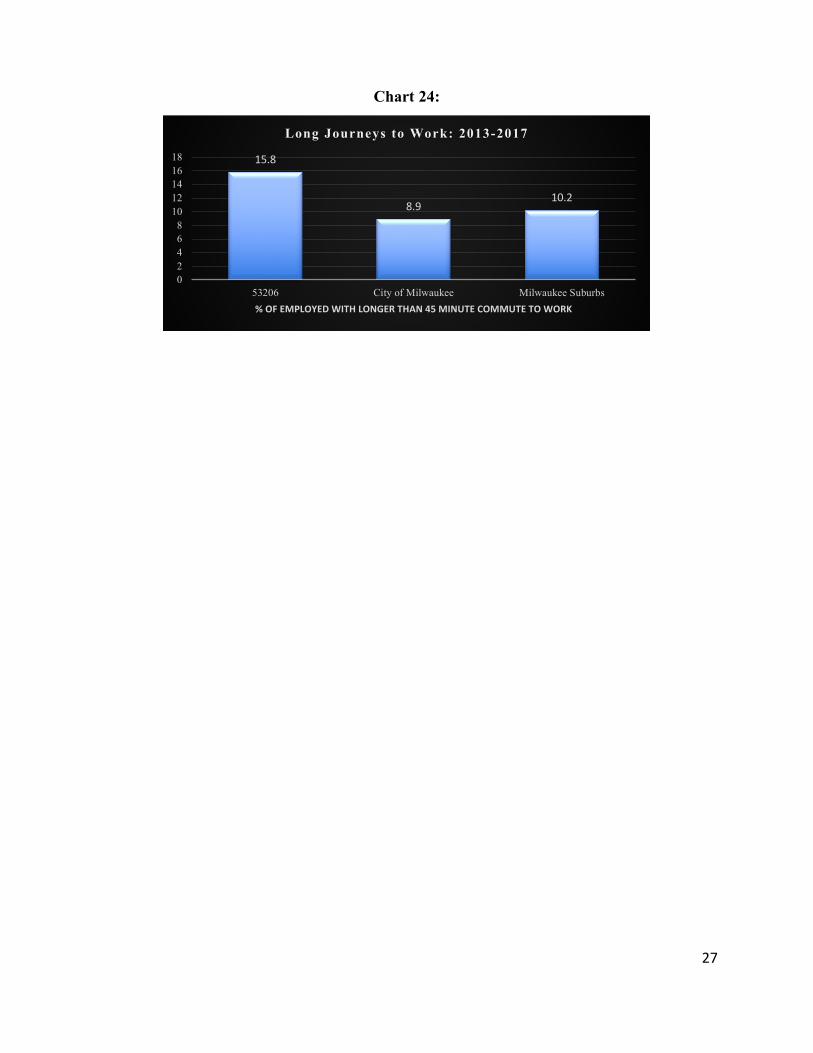
Take, for example, the question of transportation policy. As Charts 23 and 24 show, to a much

greater degree than workers throughout the city or the suburbs, that residents of 53206 are reliant

on public transit to commute to jobs. And, because regional job growth is in places far removed

Table 3:

Median Worker Earnings by Educational Attainment: 2013-2017 Both Sexes, Ages 25+

Educational Attainment Zipcode 53206 City of Milwaukee Waukesha County

Less Than High School $12,026 $21,159 $30,114 H.S. Diploma/Equivalent $21,577 $26,105 $35,612 Some College/Associate Degree $21,950 $29,686 $41,750 Bachelor’s Degree $30,919 $44,086 $61,189

22 Curiously, in 53206 –unlike the rest of the city or in Waukesha County-- there was little earnings difference between a high school graduate and a worker with “some college or an associate’s degree” in 2013-17.

26

Table 4:

Median Worker Earnings by Educational Attainment: 2013- 2017 Males, Ages 25+


Less Than High School $11,887 $24,258 $34,311 H.S. Diploma/Equivalent $21,151 $30,206 $44,518 Some College/Associate Degree $21,175 $33,836 $52,223 Bachelor’s Degree $36,667 $49,464 $78,886

from their neighborhood, residents of 53206 also have much longer commutes than workers

elsewhere in metro Milwaukee. Public transportation policy, therefore, is especially important

for workers living in 53206, to effectively link neighborhood residents to centers of employment

growth. Yet, as research by Joel Rast at the UW-Milwaukee Center for Economic Development

has shown, cuts in public transportation in Greater Milwaukee have significantly eroded the

ability of residents in inner city neighborhoods such as 53206 to access employment in suburban

job locations and have aggravated the region’s spatial mismatch.23 In short, as noted earlier,

ameliorating the labor market of 53206 and tackling the issues of joblessness and working

poverty will require new, muscular policies and strategies not only in education and training, but

in a wide range of areas: transportation, fair employment practices, and ex-prisoner re-entry, to

name just a few.

Chart 23:

23 Joel Rast, JobLines: An Analysis of Milwaukee County Transit Routes 6 and 61 (Milwaukee: UWM Center for Economic Development, 2018). Access at: https://uwm.edu/ced/wp-content/uploads/sites/431/2018/10/joblines-10-10-18.pdf; and Joel Rast, Public Transit and Access to Jobs in the Milwaukee Metropolitan Area, 2001-2014 (Milwaukee: UWM Digital Commons and UWM Center for Economic Development, 2015). Access at: https://dc.uwm.edu/cgi/viewcontent.cgi?article=1005&context=ced_pubs

21.6

8.1

1.10

5

10

15

20

25

53206 City of Milwaukee Milwaukee Suburbs% OF WORKERS COMMUTING ON PUBLIC TRANSPORTATION

Reliance on Public Transportation: 2013- 2017

27

Chart 24:

15.8

8.910.2

02468

1012141618

53206 City of Milwaukee Milwaukee Suburbs% OF EMPLOYED WITH LONGER THAN 45 MINUTE COMMUTE TO WORK

Long Journeys to Work: 2013-2017

28

POVERTY AND INCOME

In the past twenty years, scholars such as Paul Jargowsky, William Julius Wilson, Robert

Sampson, and Patrick Sharkey, among many others, have called attention to the crisis of

“concentrated poverty” in inner city neighborhoods.24 Defined by sociologists as neighborhoods

in which 40 percent or more of the residents are poor, concentrated poverty neighborhoods have

become a hallmark of urban distress and “America’s biggest problem,” in the words of one urban

analyst.25 As the authors of a Brookings Institution study put it: “Why does concentrated poverty

matter? Being poor in a very poor neighborhood subjects residents to costs and limitations above

and beyond the burdens of individual poverty.”26 “In these poorest neighborhoods,” writes

Jargowsky, “the opportunities for successful social and economic contacts are few. The problem

is exacerbated as families and businesses with better prospects relocate out of impoverished

inner-city neighborhoods, leaving many cities with abandoned and decaying cores.”27 Extensive

research has shown that “concentrated neighborhood poverty shapes everything from higher

crime rates to limited social mobility for the people –and especially the children—who live in

these neighborhoods.”28

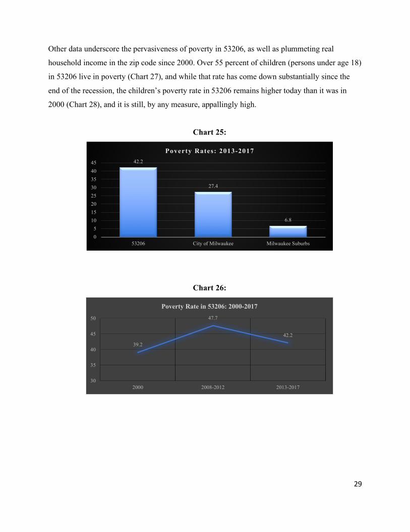
53206 is Milwaukee’s archetypical concentrated poverty neighborhood. As Chart 25 shows,

53206’s poverty rate in 2013-17 was 42.2 percent, much higher than the city-wide average and

six times greater than the poverty rate in the suburbs. The poverty rate in 53206 reached a peak

of 47.7 percent during the Great Recession and its immediate aftermath (Chart 26), but things

seem to have improved, albeit minimally, since the trough of the downturn. Nevertheless, the

poverty rate in 53206 in 2013-17 was still slightly higher than it was in 2000 (although the

difference is not statistically significant).29 By any reckoning, concentrated poverty remains a

defining feature of the social and economic landscape of Milwaukee 53206.

24 Sampson, Great American City; Wilson, The Truly Disadvantaged; Sharkey, Stuck in Place; Paul Jargowsky, Poverty and Place: Ghettos, Barrios, and the American City (New York: Russell Sage Foundation, 1997); and Paul Jargowsky, Stunning Progress, Hidden Problems: The Dramatic Decline of Concentrated Poverty in the 1990s (Washington, D.C.: Brookings Institution, 2003); Paul Jargowsky, The Architecture of Segregation: Civil Unrest, the Concentration of Poverty, and Public Policy (New York: The Century Foundation, 2015). Access at: https://tcf.org/content/report/architecture-of-segregation/?agreed=1 25 Richard Florida, “America’s Biggest Problem is Concentrated Poverty, Not Inequality.” The Atlantic, August 10, 2015. Access at: https://www.citylab.com/equity/2015/08/americas-biggest-problem-is-concentrated-poverty-not-inequality/400892/ 26 Elizabeth Kneebone, Carey Nadeau, and Alan Berube, The Re-emergence of Concentrated Poverty: Metropolitan Trends in the 2000s (Wasshington, D.C.: Brookings Institution, 2011). 27 Jargowsky, Poverty and Place, p. 1. 28 Florida, “America’s Biggest Problem.” 29 The difference in the 2000 and 2013-17 poverty rates in 53206 is not statistically significant, owing to error margins in the census survey. For all intents and purposes, the rates should be considered equal.

29

Other data underscore the pervasiveness of poverty in 53206, as well as plummeting real

household income in the zip code since 2000. Over 55 percent of children (persons under age 18)

in 53206 live in poverty (Chart 27), and while that rate has come down substantially since the

end of the recession, the children’s poverty rate in 53206 remains higher today than it was in

2000 (Chart 28), and it is still, by any measure, appallingly high.

Chart 25:

Chart 26:

42.2

27.4

6.8

05

1015202530354045


Poverty Rates: 2013-2017

39.2

47.7

42.2

30

35

40

45

50

2000 2008-2012 2013-2017

Poverty Rate in 53206: 2000-2017

30

Chart 27:

Chart 28:

As we would expect in a zip code of such concentrated poverty, median household income in

53206 significantly lags the rest of metro Milwaukee. Median household income in 53206 in

2013-17 was less than 60 percent the city of Milwaukee median, and less than 30 percent the

median household income in suburban Waukesha County (Chart 29). Almost one-fifth of 53206

households reported annual income under $10,000 a year, forming a critical mass of residents

living in extreme poverty (defined as households or individuals with income below 50 percent of

the poverty level). By contrast, only three percent of 53206 households reported annual income

above $100,000 in 2013-17, a tiny contingent of relative affluence amidst pervasive poverty and

low incomes (Charts 30 and 31). The situation in Milwaukee’s suburbs is precisely the opposite:

only 3.8 percent of suburban households had annual income below $10,000, while a whopping

33.5 percent reported income above $100,000. This is a striking illustration of the stark

economic segregation of metro Milwaukee, the geographic separation of rich and poor that

55.1

39.8

7.6

0

10

20

30

40

50

60


Children's Poverty Rate: 2013-2017

51.1

66.8

55.1

30

40

50

60

70

2000 2008-2012 2013-2017

Children's Poverty Rate in 53206: 2000-2017

31

strongly overlaps racial segregation and leaves neighborhoods like 53206 socially and

economically isolated and its residents severely disadvantaged.

Although poverty has declined slightly in 53206 since the end of the recession, median

household income has been on a continuous downward trajectory since the turn of the century.

Median household income in 53206, adjusted for inflation, dropped by 18.8 percent between

2000 and the Great Recession and its aftermath (2008-12), and then by another 7.0 percent

during the post-2012 “recovery” (Table 5). As Chart 32 graphically illustrates, real annual

income of the median household in 53206 was $30,307 in 2000; by 2013-17, that figure had

fallen to $22,877 (all figures in 2017 inflation-adjusted dollars).

Chart 29:

Chart 30:

$22,877

$38,289

$81,140

010,00020,00030,00040,00050,00060,00070,00080,00090,000

53206 City of Milwaukee Waukesha Co

Median Household Income: 2013-2017

18.1

11.1

3.8

0

5

10

15

20


Percentage of Households With AnnualIncome Under $10,000: 2013-2017

32

Chart 31:

Table 5:

Percentage Change in Real Household Income in 53206: 2000-2017

Period % change in household income

2000-2012 -18.8% 2012-2017 -7.0% 2000-2017 -24.5%

Chart 32:

Aggregate Neighborhood Income in 53206. In the late 1990s and early 2000s, leaders in

government, philanthropy, and business in Milwaukee asserted confidently that, despite low

incomes and high poverty rates, a “market-driven” revival was imminent in neighborhoods such

3.1

12.1

33.5

0

10

20

30

40


Percentage of Households With AnnualIncome Above $100,000: 2013-2017

$30,307

$24,600 $22,877

$10,000$15,000$20,000$25,000$30,000$35,000$40,000

2000 2008-2012 2013-2017

Real Median Household Income in 53206:2000-2017

in 2017 dol lars

33

as 53206.30 Following Michael Porter’s influential work on “competitive inner cities,” these

leaders insisted that while household incomes might be low in places like 53206, the population

density in such inner city neighborhoods produces surprisingly high aggregate incomes and

aggregate purchasing power. As a result, according to this approach, the inner city has a latent

“competitive advantage” in attracting businesses, particularly retail establishments drawn to

dense consumer markets.31

The claims of Porter and local acolytes were debunked at the time, and, to put it mildly,

history has not been kind to their assertion that once “urban myths” were discarded and

“untapped purchasing power” was recognized, “market-driven” growth would revive

neighborhoods like 53206 in Milwaukee.32 Indeed, Porter’s consulting group, “The Initiative for

a Competitive Inner City” (ICIC), was brought to Milwaukee with much fanfare by foundations

and business leaders in the early 2000s, to launch an “Initiative for Competitive Milwaukee;”

after just a few years, however, the Milwaukee initiative collapsed.

The aggregate “purchasing power” approach was flawed conceptually – households don’t

consume in the “aggregate,” which is why neighborhoods with large concentrations of poverty

are not hotbeds of economic development. But the analysis was also flawed empirically. As

Table 6 and Chart 33 show for 53206, declining real household income coupled with a

demographic “hollowing out” of inner city neighborhoods (which has been underway since the

1970s) has meant that real aggregate income and purchasing power have declined precipitously

in poor neighborhoods like 53206. Even if aggregate income and purchasing power were an

unrecognized “asset” of inner city neighborhoods like 53206 –a dubious formulation to begin

with-- that advantage has eroded substantially over the past decades. As Table 6 shows, real

aggregate income in 53206 has declined by over 43 percent since 2000 alone. And the zip code’s

30 See, for example, Joel Dresang, “Heart of city beats with opportunity,” The Milwaukee Journal Sentinel, January 16, 2000. 31 The seminal work is Michael Porter, “The Competitive Advantage of the Inner City,” Harvard Business Review (May-June 1995): 55-71. In a crude Milwaukee version of this approach, local researchers assembled “purchasing power profiles” of inner city neighborhoods, purporting to show that such neighborhoods actually had higher purchasing power than affluent suburban communities, and that Milwaukee’s inner city, therefore, had “a strong base of retail purchasing.” For a 53206 “purchasing power profile” in this vein, see John Pawarasat, Lois Quinn, and Frank Stetzer, “Purchasing Power Profile: Milwaukee Zipcode 53206,” (Milwaukee: UWM Digital Commons, 2001). Access at: https://dc.uwm.edu/eti_pubs/199/ 32 Among the many critiques of Porterism, see Merrill Goozner, “The Porter Prescription,” The American Prospect, (May-June 1998). Access at: https://prospect.org/article/porter-prescription; and, for a critique of Porterism in the Milwaukee context, see Marc V. Levine, The Economic State of Milwaukee’s Inner City: 1970-2000 (Milwaukee: UWM Center for Economic Development and UWM Digital Commons, 2002). Access at: https://dc.uwm.edu/cgi/viewcontent.cgi?article=1027&context=ced_pubs

34

population has declined by an estimated 60 percent since the 1970s.33 Since 2000, the number of

prime working age males living in 53206 has dropped by 28 percent. All these trends undercut

the notion that 53206 has been on the verge of a “purchasing power/density-driven” economic

revival.

Table 6:

Percentage Change in Real Aggregate Income in 53206: 2000-2017

Period % change in aggregate zipcode income

2000-2012 -30.3% 2012-2017 -18.3% 2000-2017 -43.1%

Chart 33:

Chart 34:

33 Thus, we estimate that real aggregate income in 53206 has declined by whopping 65.7 percent since 1970. See Marc V. Levine, “The Shame of Milwaukee: The Most Racial Segregated and Unequal Metro Area in America?” Presentation to the Fair Housing Council of Wisconsin, Madison, Wisconsin, April 24, 2015. Slide 32.

59,38548,630 43,293

32,868 28,210 23,827

0

20,000

40,000

60,000

80,000

1970 1980 1990 2000 2010 2017

The Depopulation of 53206:1970-2017

4,9684,342

3,594

2,000

3,000

4,000

5,000

6,000

7,000

2000 2012 2017

Disappearing Prime-Age (25-54) Males in 53206:2000-2017

35

Education, Income, and Poverty in 53206. As we documented earlier this study, educational

attainment is highly correlated with outcomes in employment and earnings, in 53206 and across

the Milwaukee region. Unsurprisingly, this is also the case with education and poverty. As Table

7 shows, in all three geographic areas for which we collected data –the city of Milwaukee,

suburban Waukesha county, and zip code 53206—there is a linear relationship between

education and poverty: the higher the level of educational attainment, the lower the individual’s

likelihood of living in poverty.34 In 53206, an individual (over age 25) who did not receive a

high school diploma was over three times likelier to live in poverty than someone with at least a

bachelor’s degree; a high school graduate in 53206 was twice as likely as a college graduate to

live in poverty.

Table 7:

Educational Attainment and Poverty in 53206 and Greater Milwaukee: 2013-17

% of persons over age 25 living in poverty, by level of educational attainment


Less Than High School 48.8 36.8 13.8 H.S. Diploma/Equivalent 31.9 22.7 6.2 Some College/Associate Degree 30.7 18.9 5.2 Bachelor’s Degree 14.0 7.2 1.6

Once again, however, there is striking evidence that “place matters” in the relationship

between education and poverty in metro Milwaukee. Even when controlling for educational

attainment, there are massive disparities in poverty rates between 53206 and elsewhere in the

region. A college graduate residing in 53206 was twice as likely to live in poverty as a

comparably educated resident of the city of Milwaukee in 2013-17, and over seven times more

likely to live in poverty than a college graduate living in Waukesha county. Similar disparities

34 In 53206, as we saw earlier in examining the relationship between education and earnings, and unlike in the rest of the city or in Waukesha County, there was little difference in the poverty rate between a high school graduate and an individual with “some college or an associate’s degree” in 2013-17.

36

exist at all education levels between 53206 and the rest of the region: for example, a high school

graduate in 53206 is five times likelier to be poor than a high school graduate in Waukesha

county. Incredibly, there is no statistical difference between the poverty rates of college

graduates in 53206 and high school dropouts in Waukesha county. Clearly, although there is no

gainsaying the importance of education, the opportunity structure in various areas of Milwaukee

is shaped by other factors as well. Put another way, “place matters.” For example, the geography

of jobs in metro Milwaukee –in particular, greater availability of entry-level jobs in Waukesha

county-- undoubtedly contributes to the very low poverty rates among high school graduates and

even dropouts there when compared to similarly educated residents of the city or 53206..

Conversely, factors such as the persistence of racial discrimination in regional labor markets, or

inequities in housing or credit markets –to name just a few likely culprits-- all deleteriously

affect the income of 53206 residents, regardless of their level of education.

37

INTERGENERATIONAL ECONOMIC MOBILITY: “STUCK IN PLACE” IN 53206?35

Another way in which “place matters” is in the degree to which neighborhood environments

shape the ability of residents and their children to achieve upward mobility. To what extent does

neighborhood affect the American credo of “equality of opportunity?” To what extent do the

children of low-income households, growing up in different neighborhoods, move up (or down)

the economic ladder? In his landmark study, Stuck in Place, sociologist Patrick Sharkey found

that “the most common experience for black families since the 1970s, by a wide margin, has

been to live in the poorest American neighborhoods over consecutive generations. Only 7

percent of white families have experienced similar poverty in their neighborhood environments

for consecutive generations.”36 In a series of landmark papers, using longitudinal “big data” from

the IRS and the Census bureau, scholars at the Harvard-based “Equality of Opportunity Project”

have demonstrated vast differences in mobility rates for the children of various household

income percentiles: between counties, metropolitan areas (“commuting zones”), census tracts,

and by racial and ethnic group.37 The Harvard data “trace the roots of today’s affluence and

poverty back to the neighborhoods where people grew up” and help the answer the question:

“Which neighborhoods in America offer children the best opportunity to rise out of poverty?”38

We have already seen, at each census measurement snapshot, the pervasiveness and

persistence of poverty in 53206. The Harvard data enable us analyze over time how children,

raised in low-income households in 53206 census tracts, have fared as they reach young

adulthood. Have they risen to a higher income percentile, indicating upward mobility, or have

they remained “stuck” at the same low-income level as their parents, evidence of

intergenerational transmission of poverty? Table 8 and Charts 35 and 36 array these results.

These charts track the 2014-15 household income percentile of children born between 1978-83,

for 53206 and for metro Milwaukee as a whole. For children born into low-income households

between 1978-83 –defined as households in the 25th percentile of the national income

distribution—we can observe their average income percentile when they reach their early and

mid-thirties in 2014-15. Table 8 shows the average young adult (ages 31-37) income percentile

35 I have, of course, borrowed the expression “stuck in place,” from Patrick Sharkey’s path-breaking book on race and the intergenerational transmission of poverty and inequality. 36 Sharkey, Stuck in Place. 37 The “Equality of Opportunity” project papers and their data are conveniently and generously available on line at: https://www.opportunityatlas.org/ 38 Ibid.

38

for black children who were born in the late 1970s and early 1980s in low-income (25th

percentile) households in census tracts located in zip code 53206. The table also includes the

estimated annual household income in dollars at those percentiles.

Table 8:

National Income Percentile in 2014-15 of Adults Born Between 1978-83 into Low-Income (25th Percentile)

Households in Census Tracts Located in 53206

Census Tract Black Male Adult HH

Income Percentile

Black Male Estimated Annual

HH Income

Black Female Adult HH

Income Percentile

Black Female Estimated

Annual HH Income

1856 25 $15,551 33 $21,599 1855 25 $15,551 33 $21,599 1854 26 $16,512 29 $19,529 87 25 $15,551 30 $20,562 86 27 $17,499 31 $21,599 85 21 $11,603 34 $24,718 84 26 $16,512 27 $17,499 68 28 $18,506 32 $22,637 66 24 $14,610 34 $24,718 65 27 $17,499 30 $20,562 64 25 $15,551 33 $23,677 47 28 $18,506 33 $23,677 46 27 $17,499 32 $22,637 45 26 $16,512 33 $23,677

In each census tract, the average household income percentile for black males in their early to

mid-30s in 2014-15 remained barely changed from the low-income percentile of the households

in which they grew up in the late 1970s or early 1980s. For example, a black male child born into

a “25th percentile” household in census tract 85 between 1978-83 had income as a young adult in

2014-15 that, on average, placed him in the 21st percentile (with an estimated annual income of

just $11,603 – extreme poverty). Clearly, for black males born and raised in 53206 in the late

1970s and early 1980s, there has been, on average, no upward mobility; as Chart 35 shows, the

average percentile for these black male children born into “25th” percentile households in 53206

between 1978-83 was…..the 25th percentile in 2014-15. (This mobility trend is worse than for

black males in metro Milwaukee as a whole who, as Chart 35 shows, rose modestly to the 30th

percentile in early adulthood).

39

Black females, born and raised in 53206, experienced slightly more upward mobility than for

black males – a gender distinction among African Americans that is consistent with what the

“Equality of Opportunity” project researchers have found nationally. Black females born

between 1978-83 into “25th percentile” households in 53206 rose, on average, to 32nd percentile

households by their young adulthood in 2014-15.

But, as Charts 35 and 36 show, racial and geographic disparities in the ability to rise out of

poverty in Milwaukee are quite pronounced. As we’ve seen, black males born in 53206 into the

25th percentile of the national income distribution in 1978-83 remained, on average, in the 25th

percentile as young adults (ages 31-37) in 2014-15 – no intergenerational mobility. On the other

hand, white males in metro Milwaukee as whole, born into the same 25th percentile in 1978-83

rose, on average, to the 45th income percentile as young adults, just slightly below the middle of

the distribution – a sign of discernible, if not dramatic, upward mobility. Put into dollar terms

(Chart 36), this means that white males (born in metro Milwaukee) and black males (born in

53206) starting out in households with identical low incomes (25th percentile) in 1978-1983 were

separated by an estimated $21,000 in annual income by the time they became young adults

(2014-15): the estimated average white male’s household income at $36,477, the black male’s at

$15,551. Tracked over 30+ years, the household income of white males born into poor

households in metro Milwaukee was now more than double that of black males born into poor

households in 53206, a clear racial and neighborhood difference in the trajectory of mobility and

opportunity.

Although black females have experienced more intergenerational mobility than males in

53206 over the past 30+ years, these same gaps by race and place exist for females. Black

females born into low-income households in 53206 in the late 1970s and 1980s experienced

much less upward mobility by young adulthood than their white counterparts born in Greater

Milwaukee, with an estimated annual income gap of $16,000 in 2014-15. In short, not only is

53206 a neighborhood of concentrated and extreme poverty, but it is also a place where it is very

difficult for residents to escape poverty. The Harvard researchers ask, “where is the land of

opportunity?” in one of the earliest papers from their pathbreaking project.39 The evidence on

intergenerational mobility is clear: 53206 is a neighborhood of deep, intergenerational poverty,

39 Raj Chetty, Nathaniel Hendren, Patrick Kline, and Emmanuel Saez, “Where is the Land of Opportunity? The Geography of Intergenerational Mobility in the United States,” NBER Working Paper No. 19843. June 2014. Access at: https://www.nber.org/papers/w19843

40

negligible intergenerational mobility for low income residents, and truncated economic

opportunity.

Chart 35:

Chart 36:

25

30

45

32

35

47

0 25 50

53206 Black Males



53206 Black Females



Income Percentile in 2014-15 of Adults Born between 1978-83 into Low-Income (25th percentile)

Households in Selected Areas

$15,551

$20,562

$36,477

$22,637

$25,759

$38,758

$0 $5,000 $10,000 $15,000 $20,000 $25,000 $30,000 $35,000 $40,000 $45,000

53206 Black Males



53206 Black Females



Estimated Average Annual Household Income in 2014-15 forChildren Born into Low-Income Households (25th percentile)

Between 1978-1983 In Selected Areas

41

HOUSING INEQUALITY

53206, as is the case in low-income inner city neighborhoods across the country, suffers from

a myriad of housing challenges: low rates of homeownership, omnipresent vacant and boarded

up housing units, and excessively high rent burdens for residents whose incomes, as we’ve

documented, have been plummeting for decades.

Homeownership is the primary means by which moderate-income U.S. households

accumulate wealth. It also often correlates with neighborhood stability and prosperity, as

homeowners, with roots in the neighborhood, are stakeholders, committed to community

improvements and quality.

As Charts 37 and 38 show, homeownership in 53206 lags well behind the rate in

Milwaukee’s suburbs, and the homeownership rate in 53206 has declined steadily since 2000 (a

product of the subprime/foreclosure crisis after 2008 as well as the secular decline of real

household income in the zip code). Just one-third of housing units in 53206 were owner-

occupied in 2013-17, compared to over 70 percent in the four-county suburbs surrounding the

city of Milwaukee. Between 2000-2017, the percentage of owner-occupied units in 53206

dropped from 38.6 percent to 33.6 percent.

CHART 37

33.6

41.9

70.7

10

20

30

40

50

60

70

80


Owner-Occupied Percentage ofHousing Units: 2013-2017

42

CHART 38:

The landscape of 53206 is also dotted with a large number of vacant housing units. Fully

one-quarter of all housing units in the zip code were vacant in 2013-17, more than double the

vacant housing rate in the city of Milwaukee, and more than five times the percentage in the

suburbs (Chart 39). Moreover, the crisis of vacant housing in 53206 has significantly worsened

since the turn of the century (Chart 40). Between 2000-2012, as 53206 was buffeted by the

subprime loan/foreclosure crisis of the Great Recession, the vacant housing rate rose sharply

(from 11.8 to 18.9 percent). Since 2012, as the secular trends of shrinking population and

declining household incomes continued to erode the housing market in 53206, the vacancy rate

rose by another seven percentage points (an almost 35 percent increase), reaching 25.5 percent of

all units in the zip code. By any reckoning, this is a visible, physical manifestation of the socio-

economic crisis that continues to grip 53206.

CHART 39:

38.6

35.7

33.6

313233343536373839

2000 2010 2017

Homeownership in 53206: 2000-2017% owner-occupied units

25.5

10.6

4.7

0

5

10

15

20

25

30


Vacant Housing: 2013-2017

43

CHART 40:

53206 is a neighborhood with a high percentage of low-income renters; thus, its residents are

particularly vulnerable to the burden of high rents. As Chart 41 shows, an extraordinary 61.7

percent of 53206’s renter households face a “high rent burden,” in which they pay over 35

percent of their income in rent. High rent burden, of course, often leads to missed payments and

evictions, and is an integral element in the daily grind of poverty in 53206.40

CHART 41:

40 A remarkable 46 percent of 53206 residents paid over half their income in gross rent in 2013-17.

11.8

18.925.5

0

5

10

15

20

25

30

2000 2008-2012 2013-2017

Percentage Vacant Housing in 53206:2000-2017

61.7

45.9

35.4

0

10

20

30

40

50

60

70

53206 City of Milwaukee Milwaukee Suburbs% HOUSEHOLDS WITH GROSS RENTS OVER 35% OF INCOME

Percentage of Renting Households with High Rent Burden

44

HEALTH INSURANCE

Neighborhoods of concentrated poverty such as 53206 have been at the forefront of the

health insurance crisis in America, with large percentages of residents among the uninsured.

Before the full implementation of the Affordable Care Act in 2014, even though many poor

residents of 53206 received some coverage through programs such as Medicaid and CHIP,41

almost 27 percent of the zip code’s adults (ages 18-54) and over 41 percent of the

neighborhood’s adult males (18-54) were without health insurance (Charts 42 and 43). Thanks to

Obamacare, however, the uninsured rate has plummeted in 53206 over the past five years: by 25

percent for all adults, and by over 31 percent for adult males.

Nevertheless, a critical mass of 53206 adults remain uninsured. In 2013-17, one-fifth of all

adults, ages 18-54, lacked health insurance, triple the percentage of uninsured in the Milwaukee

suburbs (Chart 44). Among adult males in 53206, 28.3 percent still had no health insurance in

the 2013-17 ACS survey (Chart 45). These data indicate that, while the health insurance situation

in 53206 has improved mightily since the implementation of Obamacare, a large number of

neighborhood residents face the medical and financial precariousness of living without health

insurance – another of the “cumulative disadvantages” faced by residents of this inner city

neighborhood.

CHART 42:

41 Children’s Health Insurance Program

26.7

20.2

10

15

20

25

30

35

40

2008-2012 2013-2017

Percentage of Residents Ages 18-54 Without Health Insurance in 53206: 2012-2017

45

CHART 43:

CHART 44:

CHART 45:

41.2

28.3

1015202530354045

2008-2012 2013-2017

Percentage of Male Residents Ages 18-54 Without Health Insurance in 53206: 2012-2017

20.217.1

6.7

0

5

10

15

20

25


Percentage of Residents Ages 18-54Without Health Insurance: 2013-2017

28.3

21.3

8.1

05

101520253035


Percentage of Male Residents Ages 18-54Without Health Insurance: 2013- 2017

46

EDUCATIONAL ATTAINMENT

As we saw when analyzing employment, earnings, and income trends in 53206, educational

attainment is a significant –albeit, not determinative—element in the well-being of

neighborhood residents. And residents of 53206 lag significantly behind persons living in the

city of Milwaukee as a whole and, especially, the Milwaukee suburbs, in their level of education.

Almost three-quarters of 53206 residents over the age of 25 held at least a high school diploma

in 2013-17, compared to a high school graduate rate of 83 percent in the city of Milwaukee and

almost 95 percent in the Milwaukee suburbs. This regional educational attainment gap is even

greater when we consider residents holding at least a college degree. Only 6.9 percent of 53206

residents are college graduates; this is just one-third the percentage in the city of Milwaukee and

one-sixth of the college graduate rate in the Milwaukee suburbs. The educational credentials of

53206 residents have advanced since 2000: the high school graduate percentage has risen from

57 to 72 percent, and the college graduate rate has climbed slightly from 4 percent to almost 7

percent. But growth in both percentages has been stagnant since 2008-12, and, in any event, the

educational achievement gap separating 53206 and the rest of Greater Milwaukee remains wide

– a disparity that looms large in the “concentration of disadvantage” in 53206.

CHART 46:

72.5

83.1

94.9

0

10

20

30

40

50

60

70

80

90

100

53206 City of Milwaukee Milwaukee Suburbs% OF 25+ POPULATION WITH HIGH SCHOOL DEGREE OR HIGHER

Percentage High School Graduates

47

CHART 47:

6.9

23.8

40.1

0

5

10

15

20

25

30

35

40

45

53206 City of Milwaukee Milwaukee Suburbs% OF RESIDENTS 25+ WITH BACHELOR'S DEGREE OR HIGHER

Percentage College Graduates

48

MASS INCARCERATION

In recent years, a flood of academic research has detailed the staggering rise since the 1970s

of the “carceral state” in America and the emergence of mass incarceration, especially of young

black males, as a salient element in the hyperconcentration of disadvantages facing inner cities

across the country.42 Wisconsin has been at the forefront of this surge in black male

incarceration, with the percentage of black males held in correctional facilities rising from 3.4

percent in 1970 to 11.9 percent by 2013; the incarceration rate for black males in Wisconsin is

twelve times the rate for white males43 and this racial disparity ranks among the widest in the

nation.44

In the flurry of attention to the issue of mass incarceration, 53206 has assumed special

importance, in large part thanks to the astounding claim in the documentary “Milwaukee 53206”

calling it “the zip code that incarcerates the highest percentage of black men in America.”45 This

assertion has flown across the internet46 and is routinely repeated in local journalistic accounts.47

One reporter boldly asserted that “researchers…[have] failed to locate any zip code in the nation

with a matching per-capita share of residents who are or were incarcerated.”48

These sensationalistic statements are false. While incarceration and ex-offender rates in 53206

are shockingly high (as we will document), there is no evidence that these rates are higher than

“any zip code in the nation,” and there are no studies reaching that conclusion. In fact, as we will

42 Among the many important works, see the following: Michelle Alexander, The New Jim Crow: Mass Incarceration in the Age of Colorblindness (New York: The New Press, 2010), the seminal best-seller that brought the issue of mass incarceration to wide public consciousness; Bruce Western, Punishment and Inequality in America (New York: Russell Sage Foundation, 2007); John Pfaff, Locked In: The True Cause of Mass Incarceration and How to Achieve Real Reform (New York: Basic Books, 2017); James Forman, Jr, Locking Up Our Own: Crime and Punishment in Black America (New York: Farrar, Strauss, and Giroux, 2017); and Marie Gottschalk, Caught: The Prison State and the Lockdown of American Politics (Princeton: Princeton University Press, 2015). 43 Marc V. Levine, “The Shame of Milwaukee,” Slide 29. 44 The Sentencing Project, “State by State Data on Incarceration.” Access at: https://www.sentencingproject.org/the-facts/#rankings?dataset-option=BWR 45 See “Milwaukee 53206.” Access at: https://www.milwaukee53206.com/. 46 See, for example, Alex Leichenger, “How One Milwaukee Zip Code Explains America’s Mass Incarceration Problem,” Think Progress. March 20, 2014. Access at: https://thinkprogress.org/how-one-milwaukee-zip-code-explains-americas-mass-incarceration-problem-66a6535d1c4/ ; and George Joseph, “How Wisconsin became the home of black incarceration,” The Atlantic, August 17, 2016 (accessed at: https://www.citylab.com/equity/2016/08/how-wisconsin-became-the-home-of-black-incarceration/496130/ 47 Causey, “While many want to leave Wisconsin’s most violent Zip code, these residents are staying to make it better.” 48 John Schmid, “The Unlikeliest Neighborhood.” Milwaukee Journal Sentinel, March 29, 2017. Access at: https://projects.jsonline.com/news/2017/3/29/the-unlikeliest-neighborhood.html. We assume here that the author means the share, or the percentage of residents who are or were incarcerated; per capita share of residents is a meaningless expression.

49

see shortly, there are many zip codes across the United States with higher incarceration levels

than 53206 – a sobering commentary on the pervasiveness of mass incarceration in the nation.

Measuring incarceration rates at the neighborhood level, especially if we wish to make

comparisons across the country, is not a simple or straightforward task. There is no publicly

available central data base identifying prisoners across the country by their neighborhood zip

code; and “there are no publicly available data on the exact size or composition of former

prisoners and people with felony convictions” across the country, let alone data indicating in

which specific neighborhoods these ex-offenders live.49 Issues such as recidivism (which could

lead to multiple counts of the same ex-offender), geographic mobility (what percentage of ex-

offenders still live in the zip code to which they were released), or mortality (what percentage of

ex-offenders released in a given zip code have died) pose significant methodological challenges

to researchers seeking to quantify incarceration and ex-incarceration at the neighborhood level

and to make reliable comparisons among neighborhoods across the country.50

National comparisons aside, simply counting persons in Wisconsin zip codes at a given point-

in-time who are or have been incarcerated in state prisons, is also methodologically vexing. The

files from the Wisconsin Department of Corrections (DOC) WICS51 data base are messy: they

contain no reliable zip code addresses for current inmates; in all years, many zip codes are

missing for persons under supervision of the DOC (ex-offenders paroled or on probation), an

issue especially problematic as we go back in time, to the early 2000s, when almost half the zip

codes are missing from the data; and there are no counts at all of ex-offenders in zip codes who

are no longer under the supervision of the DOC. Thus, to estimate the percentage of 53206

residents who, at a given point-in-time, are incarcerated or under the supervision of the

Wisconsin DOC involves a set of assumptions and “work-arounds” (delineated in the appendix

to this study) and the reality is that the percentage calculated is a plausible estimate rather than a

hard figure. And, of course, this final figure will also not include an indeterminate number of ex-

49 See Cherrie Bucknor and Alan Barber, The Price We Pay: Economic Costs of Barrier to Employment for Former Prisoners and People Convicted of Felonies. (Washington, D.C.: Center for Economic and Policy Research, 2016), p. 4. Access at: http://cepr.net/images/stories/reports/employment-prisoners-felonies-2016-06.pdf. For an excellent discussion of the issues surrounding how to estimate incarcerated and ex-offender populations, see Bucknor and Barber, as well as Adam Looney and Nicholas Turner, Work and Opportunity Before and After Incarceration (Washington, D.C.: Brookings Institution, 2018). Access at: http://cepr.net/images/stories/reports/employment-prisoners-felonies-2016-06.pdf 50 See Sarah K.S. Shannon, Christopher Uggen, Jason Schnittker, Melissa Thomson, Sara Wakefield, and Michael Massoglia, “The Growth, Scope, and Spatial Distribution of People With Felony Records in the United States,” Demography (2017). Vol 54: 1800-1804. 51 Wisconsin Integrated Corrections System data base.

50

offenders “off paper,” because there is no official, public inventory of such persons, at the state-

level and certainly by zip code.52 Nor, of course, does the “carceral estimate” include

neighborhood residents who are or have been incarcerated in federal prison (with no state felony

convictions and incarceration record).

However, notwithstanding these methodological obstacles, we can provide some credible

estimates on the extent of incarceration in 53206 as well as evidence on whether 53206 is,

indeed, the most incarcerated neighborhood in America. We examine these issues from several

angles. Using new and unique data sets of de-identified, confidential data from the IRS and the

Census bureau, made available by the Harvard Equality of Opportunity project as well as the

Looney-Turner study of the Brookings Institution, we can compare incarceration rates by the zip

codes and/or census tracts in which persons across the country were born and grew up.

Separately, with “point-in-time” data from various years provided by the Wisconsin DOC –the

WICS files—and with some assumptions and work arounds, we can provide estimates on the

important and controversial question of the percentage of black males in 53206 who are either

incarcerated or former state prisoners under the supervision of the Wisconsin corrections system

in various years since 2001.

52 Some research, conducted by academic staff at UW-Milwaukee’s Employment and Training Institute (ETI), purports to provide a precise count of the incarcerated and ex-offender population in 53206, Milwaukee County, and other local jurisdictions below the state level, notwithstanding the limitations of the Wisconsin DOC data. However, the ETI figures are highly problematic methodologically – even assuming that the authors somehow accessed a more complete and accurate data file than the currently available DOC numbers (they never identify their data source nor have they shared the data with scholars), and assuming that they properly accounted for issues such as recidivists, and did not double or triple count released ex-offenders. It is unclear, for example, how they arrived at their calculation of the total number of black male ex-offenders living in 53206. It appears that they simply counted all of the black male inmates who had been “formerly incarcerated” and released to 53206 over a certain period (1990-2011), assumed the ex-offenders were all still alive and residing in 53206 in 2012, added the number of current inmates who lived in 53206 before their incarceration to that total, and then divided that figure by the overall 53206 black male population in 2012 to arrive at a figure allegedly showing the percentage of the black males “presently or previously incarcerated in adult state correctional institutions” in 2012. But such an approach assuredly overcounts the number of ex-offenders living in the zip code. There is no indication that the authors verified how many of the ex-offenders were actually alive in 2012; given mortality rates as well as the normal turnover of residents moving in and out of 53206 (around half of 53206 residents change homes every five years, according to the census bureau), only a fraction of those ex-felons released to 53206 between 1990-2011 were likely still living there in 2012 –yet apparently all 1990-2011 prisoners are counted in the ETI tabulation of the 53206 “incarceration rate” in 2012. As we have noted, there are incorrect zip codes and missing data throughout DOC data sets we have obtained, but the ETI authors give no explanation of how they accounted for these data shortcomings and lacunae. In short, it appears that ETI arrived at a misleading and inflated incarceration rate for 53206 and other “sub-state” jurisdictions in Wisconsin (such as Milwaukee County) by mistakenly using a multi-year numerator of prisoners and dividing it by a single year denominator of the population. Thus, the well-traveled, and quite eye-catching map in the ETI report (p. 25), supposedly showing the precise residences in 2012 of ex-offenders in 53206, with the inflammatory conclusion that “nearly every residential block in the neighborhood had multiple numbers of ex-offenders with prison records,” is misleading (and inaccurate), as is their conclusion that over 62 percent of young black males in 53206 were “currently or previously incarcerated in state prisons.” See John Pawasarat and Lois M. Quinn, “Wisconsin’s Mass Incarceration of African American Males: Workforce Challenges for 2013,” UW-Milwaukee Employment and Training Institute, 2013, pp. 12ff, especially 23-25. Access at: https://www4.uwm.edu/eti/2013/BlackImprisonment.pdf

51

First, let’s start with the oft-repeated claim that “Milwaukee 53206” is the most incarcerated

zip code in America. Chart 48, drawn from the Looney-Turner study at Brookings, shows, by the

zip code in which individuals were born and raised, the percentage of persons (both sexes) born

between 1980-1986 who were incarcerated in 2012. Put another way, the chart shows the

incarcerated percentage of 26-32 year olds (by all accounts the most incarcerated of age cohorts)

in 2012, by their childhood zip code. In what zip codes did the highest percentage of persons,

born and raised there in the early 1980s, ultimately end up in prison in 2012? The Brookings

study examined every zip code in the country and, drawing from their data, Chart 48 below lists

the 16 zip codes with the highest incarceration rates. “Nashville 37208” heads the list, with over

14 percent of residents who were born there in the early 1980s incarcerated in 2012.

Note that “Milwaukee 53206” does not appear on the “most incarcerated list.” According to

the Brookings data, 6.75 percent of persons, born and raised in 53206 in the early 1980s, were in

prison in 2012 – an incarceration rate less than half of “Nashville 37208.” (See Chart 49).

Indeed, by this measure –“incarceration rate by childhood zip code”-- 53206 is not only not

among the nation’s most incarcerated zip codes, it is Milwaukee’s second “most incarcerated”

zip code.53

53 The Brookings study’s data does not break down persons by race or gender. (We’ll present data on race from other sources below). But, as the authors point out, since males make up over 90 percent of prison population, a “back of the envelope” way of calculating the percentage of males who were born in the zip code in the early 1980s and incarcerated in 2012 would be to estimate that the rate for males is roughly twice as high as the “all persons” figure. See Looney and Turner, “Work and Opportunity Before and After Incarceration,” p. 15. Thus, in the case of “Nashville 37208,” the estimated male incarceration rate would be 28 percent in 2012. For Milwaukee “53206,” the estimated male incarceration rate in 2012 would be 13.5 percent, a rate more or less congruent with other data we will present shortly.

52

CHART 48:

CHART 49:

From a slightly different and much more detailed angle, data from the Harvard “Equality of

Opportunity Project” enable us to examine incarceration rates by race, gender, census tract of

9.9310.0710.0810.1010.1210.2510.2610.3110.4110.4110.6010.7410.8111.02

11.4314.12

0.0 2.0 4.0 6.0 8.0 10.0 12.0 14.0 16.0

Syracuse, NY 13205Rochester, NY 14608Savannah, GA 31401

Dallas 75215Tulsa, OK 74126

Tampa, FL 33605Tulsa, OK 74106

Richmond, VA 23222Orlando, FL 32805Norfolk, VA 23504

Jacksonville, FL 32206Fort Myers, FL 33916Cincinnati, OH 45214

Waco, TX 76707Portsmouth, VA 23704

Nashville, TN 37208

U.S. Zipcodes with Highest Incarcerat ion RatesP e r c e n t a g e o f p e r s o n s b o r n b e t w e e n 1 9 8 0 a n d 1 9 8 6 ,

i n c a r c e r a t e d i n 2 0 1 2 : B y c h i l d h o o d z i p c o d e

3.71

3.77

3.86

3.95

4.61

4.69

4.71

4.93

5.10

6.24

6.75

7.09

0.0 1.0 2.0 3.0 4.0 5.0 6.0 7.0 8.0

53218

53204

53202

53216

53209

53224

53210

53233

53208

53205

53206

53212

Incarceration Rates in Milwaukee ZipcodesP e r c e n t a g e s o f p e r s o n s b o r n b e t w e e n 1 9 8 0 a n d 1 9 8 6 ,

i n c a r c e r a t e d i n 2 0 1 2 : B y c h i l d h o o d z i p c o d e

53

childhood, and the income of the household into which individuals were born. These data permit

us, for example, to answer the questions: What percentage of black males, born and raised in

low-income households54 in the census tracts located in zip code 53206, ended up in prison in

their late 20s and early 30s? And is the incarceration rate in these 53206 census tracts the highest

in the United States?

Chart 50 shows the incarceration rates in 2010 for black males who were born into low-income

(25th percentile) households between 1978-83 in census tracts located partially or entirely in

“Milwaukee 53206.” These men would have been between 27 and 32 years of age in 2010, more

or less the “prime years” for imprisonment in this era of mass incarceration according to all

research. As the chart shows, in each of the census tracts, a large percentage black boys growing

up in low-income households in the late 1970s and early 1980s in 53206 were incarcerated as

adults in 2010, ranging from 10.4 percent in tract 46 (located in the far north section of 53206) to

a staggering 33.8 percent in tract 85 (located at the southern end of the zip code). Clearly, for

young black males growing up in low-income households in 53206, the risk of becoming

ensnared in the criminal justice system in the era of mass incarceration has been very high.

CHART 50

54 Low-income households are defined, once again, as households with income that places them in the 25th percentile of the national household income distribution.

19.111.1

17.718.4

15.320.9

18.010.4

33.811.5

19.022.4

15.314.3

16.8

0.0 5.0 10.0 15.0 20.0 25.0 30.0 35.0 40.0

CT 45CT 46CT 47CT 64CT 65CT 66CT 68CT 84CT 85CT 86CT 87

CT 1854CT 1855CT 1856

Milwaukee County

Incarceration Rates in 2010 for Black Males from Low-Income Households, born between 1978-1983, in Census

Tracts Partial ly or Entirely Located in 53206

54

But as high as these 53206 incarceration levels were in 2010, they were nowhere near the

“most incarcerated in the United States.” The census tract in 53206 with the worst incarceration

rate was tract 85, at 33.8 percent; but, according to the Harvard data base, there were over 250

census tracts in the United States in which an even higher percentage of black males born into

low-income households between 1978-83 were incarcerated in 2010, in cities ranging from

Cleveland, Pittsburgh, Orlando, Los Angeles, Buffalo, Philadelphia, Richmond, Chicago, and

Dallas, to name just a few. The average census tract in 53206 posted an incarceration rate, for

black males born into poor households between 1978-83, of 17.7 percent in 2010; the Harvard

data base shows that over 3,500 of the nation’s 21,000 census tracts posted higher incarceration

rates than 17.7 percent during this period for black males. The incarceration rates in 53206 are

abysmal, but they are not unique or unprecedented: the scourge of mass incarceration for low-

income black males has enveloped neighborhoods in inner cities across the country. The stark

reality is that 53206 is one among many U.S. neighborhoods devastated by mass incarceration,

and, at least by this measure, by no means the worst case.

Finally, using the “WICS” data provided by the Wisconsin Department of Corrections, we

gauge the full extent of “carceral 53206,” by estimating the percentage of black males in the zip

code who were incarcerated or under the active supervision of the state DOC at three points-in-

time since the turn of the century: 2001, 2007, and 2013. Although this type of data is

unfortunately not available for zip codes across the country, thus ruling out comparing 53206 to

other U.S. zip codes, the DOC data permit us yearly snapshots of the overall “carceral” character

of 53206 and a view of trends in since the early 2000s. As we noted earlier, given data

limitations, this is a daunting, complicated methodological task, requiring assumptions and work

arounds, which we spell out in appendix. Following the approach of leading incarceration

researchers Shannon et al. in their national study of the geographic distribution of ex-felons,

we’ve sought “to overcome these challenges using the best available data and reasonable

assumptions by social scientific standards.” 55 But it is important to again underscore that the

figures we present are not “census-like” enumerations of the 53206 carceral population; rather,

they are plausible estimates calculated from less-than-perfect data sources.

Charts 51 and 52 and Tables 9 and 10 array estimates of the percentage of black males from

53206 who were either incarcerated in Wisconsin state prisons or under the supervision of the

55 Shannon et al., “Growth, Scope, and Spatial Distribution of People With Felonies:” 1800.

55

state Department of Corrections (on probation or parole) at the beginning of the year in 2001,

2007, and 2013. Chart 51 shows estimates for black males between the ages of 20-64; chart 52

shows estimates for the most highly incarcerated age cohort, young black men between the ages

of 25-34. We estimate that a relatively steady one-quarter of black males ages 20-64 in

“Milwaukee 53206” were in the state carceral system between 2001-2013 (Chart 51). There

appears to have been a surge, however, after 2001 in the percentage of black males ages 25-34

“in the system,” with the estimated proportion almost doubling between 2001-2007, from 24.3 to

47.2 percent. Between 2007-2013, we estimate that this figure shrank slightly to 42.3 percent.

Tables 9 and 10 show the estimated actual numbers behind these percentages.

CHART 51:

CHART 52:

23.9

28.524.1

0

5

10

15

20

25

30

35

2007 2013 2019

Estimated Percentage of Black Males , Ages 20-64, in 53206, Under Authority of Wisconsin DOC: 2001-2013

E s t i m a t e d % i n c a r c e r a t e d o r u n d e r a c t i v e c o m m u n i t y s u p e r v i s i o n

24.3

47.242.3

0

10

20

30

40

50

60

2001 2007 2013

Estimated Percentage of Black Males , Ages 25-34, in 53206, Under Authority of Wisconsin DOC: 2001-2013

E s t i m a t e d % i n c a r c e r a t e d o r u n d e r a c t i v e c o m m u n i t y s u p e r v i s i o n

56

TABLE 9:

Estimated Number of Black Males in 53206, Ages 20-64, Under Authority of Wisconsin DOC: 2001-2013

Estimated number incarcerated in state prisons or under active community supervision

*Calculated by: (Total Incarcerated + Under Supervision) / (Total Males 20-64 Living in 53206 + Incarcerated from 53206)

TABLE 10:

Estimated Number of Black Males in 53206, Ages 25-34, Under Authority of Wisconsin DOC: 2001-2013

Estimated number incarcerated in state prisons or under active community supervision

Year Incarcerated Under Supervision

Total Incarcerated +

Supervision

Total. Males 20-64 +

Incarcerated

% Carceral*

2001 319 140 459 1891 24.3% 2007 322 422 744 1576 47.2% 2013 306 332 638 1510 42.3%

*Calculated by: (Total Incarcerated + Under Supervision) / (Total Males 25-34 Living in 53206 + Incarcerated from 53206)

Two caveats should be kept in mind when interpreting these estimates of the “carceral

population” among black males in 53206. First, these estimates do not include the “off paper”

ex-incarcerated males, those no longer under the supervision of the DOC, nor do these figures

include black males from 53206 incarcerated in federal prisons. As we have noted, there are no

publicly available data on these ex-felons, and therefore no way to estimate reliably how many

live in 53206. But certainly there are some men who fall into those categories, and that would

increase the estimate of the “carceral population” of 53206 by an unspecified amount.56

56 These data gaps may not be as serious as they appear in creating an undercount in our estimates of the “carceral population.” The surge in black male incarceration in 53206, especially for the 25-34 year old age cohort, occurred in the mid-2000s; thus,

Year Incarcerated Under Supervision

Total Incarcerated +

Supervision

Total. Males 20-64 +

Incarcerated

% Carceral*

2001 766 938 1,704 7,116 23.9% 2007 796 1,215 2,011 7,055 28.5% 2013 548 895 1,443 6,012 24.1%

57

Second, as emphasized throughout this discussion, the data on which these estimates are based

have numerous gaps and potential inaccuracies. Our estimates rely on a set of assumptions that

enable us, for example, to work around the problem of missing zip code identification for a large

number of ex-prisoners as well as the rather imposing problem of having no zip code addresses

for the incarcerated population.57 Thus, it is certainly possible that what appear to be trends in

Charts 51 and 52 may be, to an unknown extent, merely artifacts of yearly variations in the

quality or completeness of the data or in the accuracy of our assumptions in a given year, rather

than a genuine trend. The estimates should be viewed as plausible and suggestive, but not

definitive (although as we point out in the appendix, data from other studies as well as the full set

of state-level data in Wisconsin suggests our estimates are credible).

Finally, what do the data tell us about the kinds of offenses for which black males in 53206

have been imprisoned in this era of mass incarceration? Michelle Alexander’s best-selling book,

The New Jim Crow, brought public attention over a decade ago not only to the rise of mass

incarceration in America, but also to the role of racial disparities in the prosecution of the “War

on Drugs” in filling prisons with young African American males; and after Alexander’s

influential analysis, the linkage between the “War on Drugs” and mass incarceration became a

staple of popular treatments of carceral America. Recent scholarly work, however, by Marie

Gottschalk58 and James Forman, Jr.,59 among others, has added considerable nuance to the topic,

pointing out that non-violent drug offenders constitute a distinct minority of prison populations

across the country, and that the rise of mass incarceration also had unmistakable roots in the

surge of violence in U.S. cities from the 1960s through the 1990s (as well as the concomitant

implementation of rigid and often harsh sentencing practices).

What do the data on the carceral population of 53206 tell us about these issues? Although, as

noted earlier, we do not have reliable information on the incarcerated males of 53206, data from

the DOC indicates that a violent felony was the most serious offense for 70.5 percent of all black

males between the ages of 20-64 incarcerated in Wisconsin state prisons in 2013 (see Chart 53).

Drug-related crimes were the most serious offense for 12.5 percent of black male prisoners.

given the relative recency of that period of incarceration, simple arithmetic suggests that the lion’s share of released prisoners living in 53206 would still be under some form of DOC supervision and thus counted in the WICS data base. 57 See appendix for details. 58 Gottschalk, Caught. 59 James Forman, Jr, “ Racial Critiques of Mass Incarceration: Beyond the New Jim Crow,” NYU Law Review, April 2012; Yale Law School, Public Law Working Paper 243: https://papers.ssrn.com/sol3/papers.cfm?abstract_id=1966018

58

There is no reason to believe that these percentages differ between “Milwaukee 53206” and the

state of Wisconsin as a whole.

We do have data on the most serious offense for ex-prisoners, living in 53206 and under the

active supervision of the Wisconsin DOC. As Chart 54 shows, violent felonies were the most

serious offenses for 37.4 percent of black males, ages 20-64, under the supervision of the DOC

and living in 53206; drug-offenses were the most serious crime for 29.2 percent of these ex-

offenders. These figures are not surprising; we would expect the “under community supervision”

population to contain a lower percentages of persons with violent offenses on their record than

the “incarcerated” population (under the logic that those convicted of violent offenses are serving

longer sentences and also less likely to be eligible for probation or parole). In any event, even

among the ex-prisoner population in 53206, a plurality had violent crimes as their most serious

offense. In short, as is the case nationally, it is misleading to attribute the wave of incarceration

in 53206 exclusively or even predominantly to the “War on Drugs;” and as criminal justice

policy moves toward strategies to reduce mass incarceration, more than simply rethinking drug-

related imprisonment will have to be on the agenda.

CHART 53

70.5

12.5

5.4 11.7

Most serious offense of Black male prisoners , ages 20-64, incarcerated in

Wisconsin state prisons: 2013

% o f t o t a l b y m o s t s e r i o u s o f f e n s e

Violent Drugs Other Public Order Property

59

CHART 54:

***

Mass incarceration is an integral component of the concentrated disadvantage of inner city

neighborhoods in U.S. cities. For young black men in these neighborhoods, especially those with

limited education, “serving time in prison has become a normal life event,” as Bruce Western

and Becky Pettit memorably put it.60 They continue: “Social and economic disadvantage,

crystallizing in penal confinement, is sustained over the life course and transmitted from one

generation to the next. This is a profound institutionalized inequality that has renewed race and

class disadvantage.”61 The effects of mass incarceration ripple through poor, segregated

neighborhoods like 53206, increasing poverty,62 undermining families and disrupting the lives of

children,63 and limiting the employment prospects of black males who have been part of the

wave of mass incarceration.64

60 Bruce Western and Becky Pettit, “Incarceration and Social Inequality,” Daedalus (Summer 2010): 8. Access at: https://www.amacad.org/sites/default/files/daedalus/downloads/10_summer_western.pdf 61 Ibid. See also Pettit and and Western, “Mass Imprisonment and the Life Course: Race and Class Inequality in U.S. Incarceration,” American Sociological Review, 69:2 (April 2004): 151-169. Access at: http://www.rci.rutgers.edu/~waltonj/404_rr/mass%20imprisonment.pdf 62 Sampson, Great American City, chapter 5. Sampson discusses the connections between concentrated poverty and what he calls “concentrated incarceration.” 63 Christopher Wildeman, “Parental Imprisonment, the Prison Boom, and the Concentration of Childhood Disadvantage,” Demography, 46:2 (May 2009): 265-280. Access at: https://www.ncbi.nlm.nih.gov/pmc/articles/PMC2831279/ 64 Devah Pager, Marked: Race, Crime, and Finding Work in the Era of Mass Incarceration (Chicago: University of Chicago Press, 2007); and Looney and Turner, Work and Opportunity Before and After Incarceration.

37.4

29.2

14.8

18.5

Most serious offense of Black male ex-offenders , ages 20-64, l iv ing in 53206, under act ive community

supervis ion of Wisconsin DOC: 2013% o f t o t a l , b y m o s t s e r i o u s o f f e n s e

Violent Drugs Other Public Order Property

60

Mass incarceration is now woven into the community fabric of 53206, a “normal life event”

that has become one of the “cumulative disadvantages” of the neighborhood. As we have shown,

young black men born into low-income households in 53206 in the early 1980s had a roughly

one in five chance of being incarcerated 30 years later. By 2013, roughly two in five black men

between the ages of 25-34 in 53206 were either incarcerated in state prisons or released and

under the active supervision of the state Department of Corrections. Although it is inaccurate to

label 53206 the “most incarcerated zip code in America,” that hyperbole does not diminish the

gravity of how mass incarceration has “crystallized” social and economic disadvantage in this

beleaguered Milwaukee neighborhood.

61

CONCLUSION

Milwaukee 53206 remains a neighborhood of entrenched, pervasive, cumulative, and

interconnected disadvantages. No matter what social or economic indicator we explore –

employment, earnings, poverty, household income, housing, demographic growth, or

incarceration—the statistics for 53206 are almost incomprehensibly grim. Fewer than half of

prime working age men in 53206 are employed (and fewer than half of the employed men hold

full-time, full-year jobs); adjusted for inflation, median male worker earnings have declined 33

percent since 2000, and the income of the median household in 53206 has dropped by almost 25

percent; over 42 percent of neighborhood residents live below the poverty line (including 55

percent of all children); almost 30 percent of residents have abandoned the zip code since 2000

(and an estimated 61 percent have left since 1970); one-quarter of all housing units in 53206 are

vacant; almost half of households in the zip code spend more than half of their income just on

rent; and an estimated 42 percent of black males from 53206 between the ages of 25 and 34 are

in state prison or are ex-inmates now under the “active community supervision” of the Wisconsin

Department of Corrections.

Milwaukee 53206 is a neighborhood of low employment rates, low wages, shrinking income,

high poverty, poor housing, and mass incarceration. And these are just a few of the more

stunning indicators of 53206 distress, all of them interconnected and all of them reinforcing one

another into something of a durable ecosystem of neighborhood disadvantage.65 Despite some

modest improvements in 53206 on indicators such as employment and poverty since the end of

the Great Recession, and despite the hard work of numerous groups and community leaders in

the zip code, this “ecosystem of disadvantage” --built on segregation, racial inequality, and

historical patterns of discrimination, disinvestment, and official neglect-- remains largely intact.

What’s more, evidence presented in this study suggests that the disadvantages concentrated in

53206 affect not only the daily lives of residents but also opportunities for upward mobility in

the future. Black males who were born over 30 years ago into low-income households in 53206,

remained poor as they reached young adulthood, unlike their white counterparts who were born

elsewhere in metro Milwaukee and, on average, rose from their low-income origins to approach

65 The concepts of “interlocking structures” and the “enduring neighborhood effect” are comprehensively discussed in Robert Sampson’s The Great American City, a brilliant anatomy of inner city disadvantage in Chicago.

62

the middle of the income distribution. Starting at identical household income levels when they

were children, by 2015 the average annual income of a young adult black male born in 53206

was only 42 percent that of his white counterpart born elsewhere in Milwaukee ($15, 551 to $36,

477). For the young boys of 53206, intergenerational economic mobility has been not just

elusive, but virtually non-existent.66

Even the impact of factors associated with economic opportunity – such as work and

education—are refracted through and ultimately vitiated by the enduring structure of

neighborhood disadvantage concentrated in 53206. For example, even among those working-age

residents of 53206 holding jobs, over one-fifth report income below the official poverty line, a

level of working poverty that far exceeds the rate elsewhere in metro Milwaukee. More startling

still, nearly 10 percent of the 53206 residents holding full-time, year-round jobs report poverty-

level incomes. Although it is a truism that jobs are a sine qua non for any kind of improvement

in neighborhood life, “making work pay” –let alone, generating family-supporting jobs

accessible to neighborhood residents-- remains elusive in 53206. In this fashion, the challenge of

stagnant wages and shrinking numbers of “middle-class” jobs in the larger economy67 takes an

especially acute form in the ecosystem of disadvantage that marks “Milwaukee 53206.”

Similarly, the generally salutary impact of education on economic advancement is also

refracted through the enduring, concentrated “neighborhood effects” in 53206. On the one hand,

the relationship between educational attainment and better outcomes in employment, earnings,

and poverty rates holds in 53206 as elsewhere: as we would expect, 53206 residents with college

degrees have higher employment rates and earnings, and lower poverty rates than high school

graduates; in turn, 53206 high school graduates do better than 53206 high school dropouts. No

surprises in this confirmation that “education matters.”

But, on the other hand, when we control for education, we see the stark “spatial

disadvantages” of 53206. On average, high school dropouts in the Milwaukee suburbs have

virtually the same employment rate as residents of 53206 with some college or an associate’s

degree. Among the employed, the median earnings of a high school dropout in Waukesha

66 And, as we document in this study, the rate of intergenerational mobility for black females born into low-income households in 53206 has been only marginally better than for black males, and significantly lower than for white females born elsewhere in Milwaukee into low-income households. 67 In the vast literature on the polarization of jobs and wage stagnation, see David Autor, “The Polarization of Job Opportunities in the U.S. Labor Market: Implications for Employment and Earnings.” Center for American Progress, April 2010. Access at: https://economics.mit.edu/files/5554

63

County are the same as for a 53206 college graduate. And the poverty rate for a Waukesha

County high school dropout is less than half the rate of a 53206 resident with some college or an

associate’s degree. Education matters – but its impact on economic opportunity in 53206 is

powerfully mediated by what sociologist Patrick Sharkey calls “the spatial organization of

America’s stratification system [that] affects the life chances, and the economic trajectories, of

different segments of the population in ways that maintain, and reinforce, inequality.”68

In the last analysis, the plight of 53206 is inextricably connected to the persistence in

Milwaukee of what urbanist Paul Jargowsky calls “the architecture of segregation.”69

Incremental progress certainly has occurred in the neighborhood over the past decade, thanks to

energetic community initiatives such as Amani United, as well as the trickling-down into 53206

of the broader, post-recession economic recovery occurring in the city and region. Residents

have higher levels of educational attainment than they did in 2000, let alone a generation ago.

But, overall, the economic and social gains have been small, the deep inequalities and

neighborhood isolation linger, and until the architecture of segregation and the legacy of racial

injustice in the region are seriously and comprehensively addressed, “Milwaukee 53206” will

remain a neighborhood of concentrated disadvantage and truncated economic opportunity.

68 Patrick Sharkey, “Neighborhoods, Cities, and Economic Mobility,” RSF: The Russell Sage Foundation Journal of the Social Sciences, Vol. 2, Number 2 (May 2016): 159. 69 Jargowsky, The Architecture of Segregation, (2015).

64

APPENDIX: Methodology for Estimating the Carceral Population of Milwaukee 53206

As we noted in the body of this study, gauging the number of residents at the neighborhood level who are incarcerated or formerly incarcerated is challenging. Available data sources are plagued by missing, incomplete, or inaccurate data, and for certain carceral categories –such as ex-prisoners “off paper” and no longer under the active supervision of the criminal justice system—there are no public data available at all.

To generate estimates of the carceral population of “Milwaukee 53206,” we obtained two data

files from the Wisconsin Department of Corrections (DOC): 1) Annual “Point in Time” enumerations of incarcerated population in state prisons; and 2) Annual “Point in Time” enumerations of the state population under active supervision by the DOC. All these data are available in the “Wisconsin Integrated Corrections System” data base, or WICS.70

Although the WICS data are the best source for analyzing carceral levels in Wisconsin, they

are far from perfect. The WICS data provide complete “point in time” enumerations of inmates in state prisons and ex-prisoners under active supervision by the DOC for the entire state, by race, ethnicity, gender, and age. Those counts appear accurate and complete. But, in each year between 2001-2013, between 15-47 percent of the zip codes are missing for the “under supervision” population. And because of inaccuracies in the data, the DOC does not include zip codes at all in the current inmate file.

Here’s the somewhat complicated process of how we attempted to work around these gaps in

the data to arrive at estimates of the carceral population in various age cohorts among African American males from Milwaukee 53206. First, we tabulated the total number of black males, by age cohorts, among the “incarcerated” and “under supervision” population, from the “point in time” files for 2001, 2007, and 2013 for the state of Wisconsin as a whole. Second, we tabulated the number of black males, by age cohorts, among the “under supervision” population in 53206 (recognizing, because of missing zip codes in the state tabulation, that this was an incomplete count).

To deal with the “undercount” in the 53206 “under supervision” tabulation, we then calculated

the ratio of 53206 black males under supervision to the Wisconsin total of black males under supervision. We next took this ratio and applied it to the population missing zip codes, on the assumption that the distribution of the “unknown” zip codes was the same as the ones for which we had zip code identification. Finally, we allocated this additional number to the tabulation of the under supervision population of black males, by age cohorts, in 53206. Although this assumption contains obvious error margin possibilities –most notably, that the ratio of 53206-to-the-entire-state differs in the missing zip codes from the known zip codes-- we believe that assuming some portion of the missing zip code population are 53206 residents is plausible and credible, and brings us closer to a reliable count of the “under supervision” population in 53206. 70 On line lists of inmates in state prisons and ex-prisoners under active community supervision are available through the “General Public- Offender Search” web site maintained by the State of Wisconsin. But this site also has a large amount of missing data, and the aggregate number of inmates and ex-offenders listed on the site does not match what we know of number for state as a whole as well as for individual zip codes; the counts are much too low. Thus, the data on this site are not adequate for serious analysis of the carceral population in Wisconsin, not at the state level and especially not in smaller units (counties, cities, or zip codes).

65

To estimate the percentage of “incarcerated” from 53206, we made another assumption: that the 53206 “share” of the Wisconsin black male incarcerated population was the same as the 53206 percentage of the Wisconsin “under supervision” population (among black males). We then applied that percentage to the full count of Wisconsin’s “point-in-time” inmate population to arrive at an estimate at the number of inmates in 53206. Thus, to give a concrete example: our estimate for 2001 was that 7.9% of all black males in Wisconsin under the community supervision of the DOC between the ages of 20-64 lived in 53206. To estimate the number of black male state prison inmates from 53206 in 2001, we took that percentage (7.9%) and applied it to the state total of black male inmates (9,725) to estimate that there were 766 black males ages 20-64 incarcerated in Wisconsin state prisons in 2001 (see Table 9 of this study).

Once again, assumptions such as these introduce important error margins to our calculations –and readers are cautioned to keep those in mind. But in lieu of accurate, enumeration-style counts of prisoners or ex-inmates at the zip code level, these “work arounds” enable us to come up with plausible and credible estimates of the carceral population in 53206. The plausibility of our methodology can be gauged by comparing state-level calculations of the percentage of black males who were prisoners or under DOC community supervision to our estimates of the 53206 black male carceral population. There are no assumptions or work arounds in the state calculations; at the state level, the WICS data are census-like enumerations. Yet, as the table below shows, the percentages of black males in both the 20-64 and 25-34 age cohorts at the state-level and for 53206 are relatively comparable, increasing our confidence in the accuracy of our 53206 estimates. The biggest discrepancy appears to be in the 25-34 year old age group, where in 2007 and to a lesser extent 2013, the 53206 percentages are much higher than for the state of Wisconsin as a whole. But given the concentrated disadvantage for young black men in 53206 as well as high crime rates in the zip code, the higher carceral rates for this age cohort in Milwaukee 53206 seem entirely reasonable.71

Percentage of Black Males Incarcerated in State Prisons

or Under Active Community Supervision of DOC:

State-Wide Wisconsin and “Milwaukee 53206” Year Age Cohort

Wisconsin 53206

2001 20-64 28.7 23.9 25-34 22.9 24.3 2007 20-64 24.7 28.5 25-34 34.2 47.2 2013 20-64 22.6 24.0 25-34 36.4 42.3

71 These estimates are generally consistent with findings in national studies, further bolstering their credibility. Pettit and Western, “Mass Imprisonment and the Life Course,” estimated in 2000 that around 32% of “non-college” black males were or had been incarcerated (22% of all black males); Shannon et al., “Growth, Scope, and Spatial Distribution of People With Felonies,” estimated in 2017 that about 33% of black males were incarcerated or ex-prisoners.

66

SOURCES FOR CHARTS AND TABLES Chart 1: U.S. Bureau of the Census, American Community Survey, 2013-17 5-Year Estimates (Hereafter referred to as “ACS”). Table S2301: Employment Status. Chart 2: Same as Chart 1. Chart 3: ACS, 2013-17. Table B23001: Sex By Age By Employment Status for the Population 16 Years and Over. Chart 4: Same as Chart 3. Chart 5: ACS, 2013-17 and 2008-12, Table S2301. U.S. Bureau of the Census, Decennial Census. Table QT-P24: Employment Stats by Sex: 2000. Census 2000 Summary File (SF3) Sample Data. Chart 6: Same as Chart 5. Chart 7: ACS, 2008-12, and 2013-17. Table B23001; Census 2000 SF3, Table QT-P24. Chart 8: Social Security Administration, Research Statistics, and Policy Analysis. OASDI Beneficiaries by State and Zip Code, 2017. Chart 9: ACS, 2013-17. Table C18120: Employment Status By Disability Status. Chart 10: Same as Chart 9. Chart 11: ACS, 2013-17. Table B23027: Full-Time, Year-Round Work Status in the Past 12 Months By Age for the Population 16 Years And Over. Table 1: ACS, 2013-17. Table S2301: Employment Status. Chart 12: Same as Chart 11. Chart 13: Same as Chart 11. Chart 14: Same as Chart 11. Chart 15: ACS, 2013-17. Table S2303: Work Status in the Past 12 Months. Chart 16: ACS, 2013-17. Table S2001: Earnings in the Past 12 Months (in 2017 inflation-adjusted dollars). Chart 17: Same as Chart 16.

67

Chart 18: Same as Chart 16. Chart 19: ACS, 2008-12 and 2013-17. Table S2001: Earnings in the Past 12 Months (in 2017 inflation-adjusted dollars); Census 2000 SF3 Data. Table P085: Median Earnings in 1999 (Dollars) by Sex for the Population 16 Years and Over with Earnings. Chart 20: Same as Chart 19. Table 2: Same as Chart 19. Chart 21: ACS, 2013-17. Table B23024: Poverty Status in the Past 12 Months by Disability Status by Employment Status for the Population 20 to 64 Years. Chart 22: ACS, 2013-17. Table S1703: Selected Characteristics of People at Specified Levels of Poverty in the Past 12 Months. Table 3: ACS, 2013-17. Table S2001: Earnings in the Past 12 Months (in 2017 inflation-adjusted dollars). Table 4: Same as Table 3. Chart 23: ACS, 2013-17. Table S0802: Means of Transportation to Work by Selected Characteristics. Chart 24: Same as Chart 23. Chart 25: ACS, 2013-17. Table S1703: Selected Characteristics of People at Specified Levels of Poverty in the Past 12 Months. Chart 26: ACS, 2008-12 and 2013-17. Table S1703: Selected Characteristics of People at Specified Levels of Poverty in the Past 12 Months. Census 2000 SF3. Table P087: Poverty Status in 1999 By Age. Chart 27: ACS, 2013-17. Table S1703: Selected Characteristics of People at Specified Levels of Poverty in the Past 12 Months. Chart 28: ACS, 2008-12 and 2013-17. Table S1703: Selected Characteristics of People at Specified Levels of Poverty in the Past 12 Months. Census 2000 SF3. Table P087: Poverty Status in 1999 By Age. Chart 29: ACS, 2013-17. Table B19013: Median Household Income in the Past 12 Months (in 2017 inflation-adjusted dollars). Chart 30: ACS, 2013-17. Table S1901: Income in the Past 12 Months (in 2017 inflation-adjusted dollars).

68

Chart 31: Same as Chart 30 Table 5: ACS, 2008-12 and 2013-17. Table B19013: Median Household Income in the Past 12 Months; Census 2000 SF3. Table HCT012: Median Household Income in 1999 (Dollars). Chart 32: Same as Table 5. Table 6: ACS, 2008-12 and 2013-2017. Table B1925: Aggregate Household Income in the Past 12 Months; Census 2000 SF3. Table HCT013: Aggregate Household Income in 1999 (Dollars). Chart 33: U.S. Bureau of the Census, Census of Population and Housing, 1970, 1980, and 1990; Census 2000 SF1. Table P001: Total Population; and ACS, 2008-12 and 2013-17. Table B01003: Total Population. Chart 34: ACS 2008-2012 and 2013-17. Table S0101: Age and Sex; Census 2000 SF1. Table P012: Sex by Age. Table 7: ACS, 2013-2017. Table S1703: Selected Characteristics of People at Specified Levels of Poverty in the Past 12 Months. Table 8: Harvard University, Opportunity Insights Atlas. Data available at: https://www.opportunityatlas.org/ Chart 35: Same as Table 8 Chart 36: Same as Table 8 Chart 37: ACS, 2013-2017. Table B25003. Tenure: Occupied Housing Units. Chart 38: ACS, 2013-2017. Table B25003. Tenure: Occupied Housing Units; Census 2000 SF1 and 2010 Census Summary File 1. Table DP-1. Profile of General Population and Housing Characteristics: 2000 and 2010. Chart 39: ACS, 2013-2017. Table B25002: Occupancy Status. Chart 40: ACS, 2008-2012 and 2013-2017. Table B25002: Occupancy Status; Census 2000 SF1. Table DP-1. Profile of General Population and Housing Characteristics: 2000. Chart 41: ACS, 2013-2017. Table B25070: Gross Rent as a Percentage of Household Income in the Past 12 Months. Chart 42: ACS, 2008-2012 and 2013-2017. Table B27001: Health Insurance Coverage Status By Sex By Age. Chart 43: Same as Chart 42

69

Chart 44: ACS, 2013-2017. Table B27001: Health Insurance Coverage Status By Sex By Age. Chart 45: Same as Chart 44. Chart 46: ACS, 2013-2017. Table S1501: Educational Attainment. Chart 47: Same as Chart 46. Chart 48: Data-base made available by Adam Looney and Nicholas Turner (Brookings Institution) as part of report, Work and Opportunity Before and After Incarceration. Data available at: https://www.brookings.edu/research/work-and-opportunity-before-and-after-incarceration/ Chart 49: Same as Chart 48. Chart 50: Harvard University, Opportunity Insights Atlas. Data available at: https://www.opportunityatlas.org/ Chart 51: State of Wisconsin, Department of Corrections (DOC), Wisconsin Integrated Corrections System Files. Point-in-time files of inmates and ex-prisoners under the active community supervision of the DOC: 2001, 2007, 2013. Chart 52: Same as Chart 51 Table 9: Same as Chart 51 Table 10: Same as Chart 51 Chart 53: Same as Chart 51 Chart 54: Same as Chart 51

Milwaukee 53206: The Anatomy of Concentrated …

Documents

Transcript of Milwaukee 53206: The Anatomy of Concentrated …