MIKE ZERO Mesh Generator Step-by-step training...

MIKE by DHI 2012

MIKE ZERO

Mesh Generator

Step-by-step training guide

2012-09-21/MESH_GENERATOR_STEP_BY_STEP.DOCX/AJS/NHP/2012_StepbySteps.lsm

Agern Allé 5 DK-2970 Hørsholm Denmark Tel: +45 4516 9200 Support: +45 4516 9333 Fax: +45 4516 9292 [email protected] www.mikebydhi.com

i

CONTENTS

MIKE Zero Mesh Generator Step-by-step guide

1 INTRODUCTION .............................................................................................. 1

1.1 Background ............................................................................................................................. 1 1.2 Objective ................................................................................................................................. 1 1.3 General Considerations before Creating a Computational Mesh ............................................ 2

1.3.1 Courant number ....................................................................................................................... 3 1.4 Remarks ................................................................................................................................... 3 1.5 Concepts .................................................................................................................................. 4 1.6 Mesh File ................................................................................................................................. 4

2 BATHYMETRY DATA .................................................................................... 7

2.1 Computational Grid ................................................................................................................. 7

2.2 Water Depths ........................................................................................................................... 7

2.3 Boundary Data ........................................................................................................................ 8 2.4 Background Images ................................................................................................................. 8

3 INITIAL COMPUTATIONAL MESH.............................................................. 9

3.1 Creating the Workspace .......................................................................................................... 9 3.2 Digitize Model Boundary ...................................................................................................... 14

3.3 Import Model Boundaries ..................................................................................................... 15 3.4 Specification of Domain ....................................................................................................... 16 3.4.1 Editing land boundary ........................................................................................................... 16

3.4.2 Adjusting the boundary data into a domain that can be triangulated .................................... 18 3.5 Specification of Boundaries .................................................................................................. 19

3.6 Mesh Generation ................................................................................................................... 21

3.7 Analysis ................................................................................................................................. 22

3.8 Smoothing the Mesh ............................................................................................................. 24

4 INITIAL BATHYMETRY .............................................................................. 27

4.1 Importing Scatter Data .......................................................................................................... 27 4.2 Interpolating Scatter Data ..................................................................................................... 28 4.3 Analysing the Mesh............................................................................................................... 29 4.4 Exporting the Mesh ............................................................................................................... 29 4.5 Viewing the Mesh ................................................................................................................. 29

4.6 Next Steps ............................................................................................................................. 31

ii MIKE Zero

5 MESH FOR REGIONAL WAVE SIMULATION .......................................... 33

5.1 Modifying the Land Boundary .............................................................................................. 33 5.2 Increasing Resolution ............................................................................................................ 35 5.2.1 Simple refinement of mesh ................................................................................................... 35

5.2.2 Using smaller maximum element areas ................................................................................ 36 5.3 Interpolating Bathymetry ...................................................................................................... 36 5.4 Refine Mesh in Shallow Areas ............................................................................................. 39 5.5 Influence of Mesh Resolution on Simulation Results ........................................................... 41

6 MESH FOR LOCAL WAVE SIMULATION ................................................. 43

6.1 Available Data ...................................................................................................................... 43 6.2 Modifying the Land Boundary .............................................................................................. 44

6.3 Using Polygons in Mesh Generation .................................................................................... 45 6.4 Prioritize Scatter Data ........................................................................................................... 48 6.5 Updating Mesh Bathymetry Using New Scatter Data .......................................................... 51

6.6 Influence of Bathymetry on Simulation Results ................................................................... 54

7 MESH FOR LONGSHORE CURRENT SIMULATION ............................... 57

7.1 Defining Polygons for Customization .................................................................................. 57

7.1.1 Defining quadrangular elements ........................................................................................... 58 7.1.2 Interpolating bathymetry ....................................................................................................... 60 7.2 Neighbouring Quadrangular Element Areas ......................................................................... 64

7.2.1 Two adjacent areas ................................................................................................................ 65 7.2.2 Complex combination of quadrangular areas ....................................................................... 69

8 IMPACT OF TIDAL FLOW ........................................................................... 75

8.1 Creating the Land Boundary ................................................................................................. 76 8.1.1 Redistribute vertices on arc ................................................................................................... 76 8.2 Specification of Domain ....................................................................................................... 80

8.3 Using Break Lines ................................................................................................................. 82 8.4 Increasing the Model Domain ............................................................................................... 85 8.5 Simulation Results ................................................................................................................ 88

9 PHASE II OF PREVIOUS INVESTIGATION ............................................... 91

9.1 Modifying Existing Mesh File .............................................................................................. 93

9.1.1 Moving mesh nodes .............................................................................................................. 93 9.1.2 Re-triangulate selected region ............................................................................................... 95 9.1.3 Adding node points ............................................................................................................... 96 9.1.4 Deleting mesh nodes ............................................................................................................. 97

9.1.5 Interpolating bathymetry ....................................................................................................... 98 9.1.6 Modifying properties of single mesh node ........................................................................... 99 9.1.7 Evaluating change ............................................................................................................... 100 9.2 Re-establishing .mdf File for Existing Mesh ...................................................................... 100 9.2.1 Extract node point data from mesh ..................................................................................... 101

9.2.2 Import node points .............................................................................................................. 102 9.2.3 Define boundaries ............................................................................................................... 104

iii

9.2.4 Create mesh ......................................................................................................................... 108

9.2.5 Interpolate mesh .................................................................................................................. 108

iv MIKE Zero

Introduction

Step-by-step training guide 1

1 INTRODUCTION

This Step-by-step training guide relates to the bathymetry around Thorsminde

harbour on the west coast of Denmark.

Figure 1.1 Thorsminde, Denmark

Setting up a mesh includes appropriate selection of the area to be modelled,

adequate resolution of the bathymetry, flow, wind and wave fields under

consideration and definition of codes for open and land boundaries. Furthermore,

the resolution in the geographical space must also be selected with respect to

stability considerations.

1.1 Background

Thorsminde Harbour experienced problems with siltation in the harbour entrance.

Some investigations were therefore made to assess the problems and different

layouts were tested. As a result, a new harbour layout was carried out resulting in

lower maintenance costs.

1.2 Objective

The objective of this Step-by-step training guide is to use the Mesh Generator to

create various meshes, each designed to apply for a special modelling task.

The bathymetry mesh is created from scratch and optimized to a satisfactory level.

Attempts have been made to make this exercise as realistic as possible although

some short cuts have been made with respect to the data input. This mainly relates

to quality assurance and pre-processing of raw data to bring it into a format readily

Mesh Generator

2 MIKE Zero

accepted by the MIKE Zero software. Depending on the amount and quality of the

data sets this can be a tedious, time consuming but indispensable process. For this

example guide the ‘raw’ data has been provided as standard ASCII text files and

encrypted MIKE C-MAP files.

The files used in this Step-by-step training guide can be found in your MIKE Zero

installation folder. If you have chosen the default installation folder, you should

look in:

C:\Program Files (x86)\DHI\2012\MIKE Zero\Examples\MIKE_Zero\MeshEdit\Torsminde

Please note that all future references made in this Step-by-step guide to files in the

examples are made relative to above-mentioned folder.

References to User Guides and Manuals are made relative to the default

installation path:

C:\Program Files (x86)\DHI\2012\MIKE Zero\Manuals\

1.3 General Considerations before Creating a Computational Mesh

The resulting computational grid file in Flow Model FM is an ASCII file with

extension (.mesh) that includes information of the geographical position and water

depth at each node point in the mesh. The file also includes information about the

node connectivity of the triangular and quadrangular elements. All the

specifications for generating the mesh file are saved in a Mesh Definition File with

extension (.mdf), which can be modified and re-used.

The bathymetry and mesh file should

1 describe the water depths in the model area,

2 allow model results with a desired accuracy, and

3 give model simulation times acceptable to the user.

To obtain this, you should aim at a mesh:

• with triangles without small angles (the perfect mesh has equilateral triangles)

• with smooth boundaries

• with high resolutions in areas of special interest

• based on valid xyz data using the same chart datum

Large angles and high resolutions in a mesh are contradicting with the need for

short simulation times, so the modeller must compromise his choice of

triangulation between these two factors.

In areas with a pre-dominant flow direction it may be feasible to apply a

quadrangular mesh in order to reflect the flow pattern more accurately.

Introduction


1.3.1 Courant number

The Courant–Friedrichs–Lewy condition (CFL condition) is a necessary condition

for convergence while solving certain partial differential equations. It arises when

explicit time-marching schemes are used for the numerical solution. As a

consequence, the time step must be less than a certain time in many explicit time-

marching computer simulations; otherwise the simulation will produce wildly

incorrect results.

The basic CFL number for wave simulations has the following form:

SW

tCFL c

x

(1.1)

Where c is the wave celerity, ∆t is the time step and ∆x is the spatial resolution.

For flow modelling the CFL number is influenced explicitly by the water depth as

well:

HD

t tCFL g h u g h v

x x

(1.2)

Where g is gravity, h is the water depth, u and v are the velocity components in the

x- and y-direction, t is the time step and x is the spatial resolution.

The resolution of the mesh, combined with the water depths and chosen time-step

governs the Courant numbers in a model set-up. The maximum Courant number

shall be less than 1.0. So the simulation times dependency on the triangulation of

the mesh, relates not only to the number of nodes in the mesh, but also the

resulting Courant numbers. As a result of this, the effect on simulation time of a

fine resolution at deep water can be relatively high compared to a high resolution

at shallow water.

1.4 Remarks

The time spent on creating a reliable mesh before starting the actual simulations is

well spent. However it should be anticipated that the first simulations may give

rise to the need of further modifications of the mesh as the results are analysed and

may found lacking in detail.

Before finalising a project you should anticipate several re-runs of the standard

mesh commands: generate, smooth and interpolate.

Mesh Generator

4 MIKE Zero

1.5 Concepts

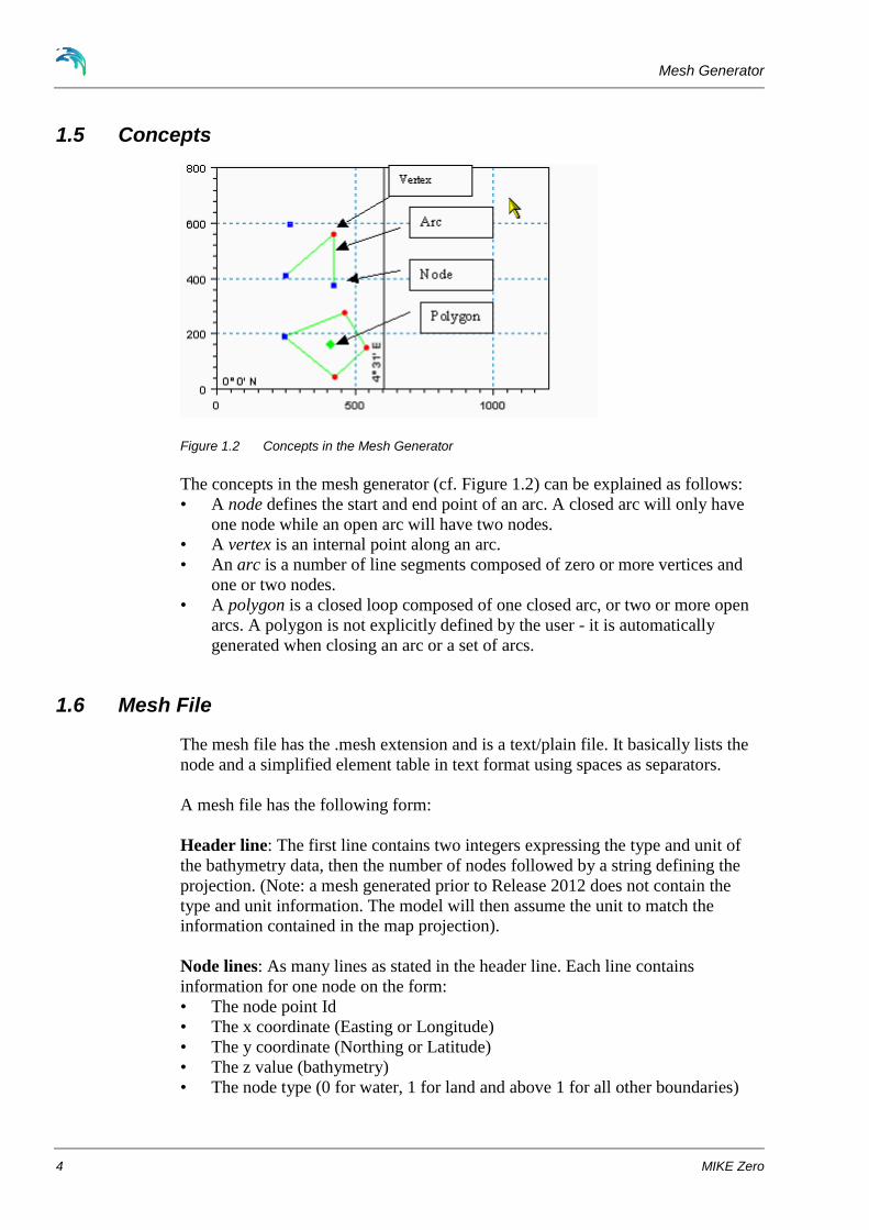
Figure 1.2 Concepts in the Mesh Generator

The concepts in the mesh generator (cf. Figure 1.2) can be explained as follows:

• A node defines the start and end point of an arc. A closed arc will only have

one node while an open arc will have two nodes.

• A vertex is an internal point along an arc.

• An arc is a number of line segments composed of zero or more vertices and

one or two nodes.

• A polygon is a closed loop composed of one closed arc, or two or more open

arcs. A polygon is not explicitly defined by the user - it is automatically

generated when closing an arc or a set of arcs.

1.6 Mesh File

The mesh file has the .mesh extension and is a text/plain file. It basically lists the

node and a simplified element table in text format using spaces as separators.

A mesh file has the following form:

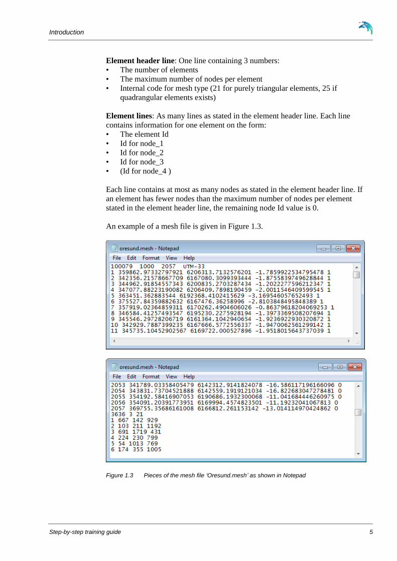
Header line: The first line contains two integers expressing the type and unit of

the bathymetry data, then the number of nodes followed by a string defining the

projection. (Note: a mesh generated prior to Release 2012 does not contain the

type and unit information. The model will then assume the unit to match the

information contained in the map projection).

Node lines: As many lines as stated in the header line. Each line contains

information for one node on the form:

• The node point Id

• The x coordinate (Easting or Longitude)

• The y coordinate (Northing or Latitude)

• The z value (bathymetry)

• The node type (0 for water, 1 for land and above 1 for all other boundaries)

Introduction


Element header line: One line containing 3 numbers:

• The number of elements

• The maximum number of nodes per element

• Internal code for mesh type (21 for purely triangular elements, 25 if

quadrangular elements exists)

Element lines: As many lines as stated in the element header line. Each line

contains information for one element on the form:

• The element Id

• Id for node_1

• Id for node_2

• Id for node_3

• (Id for node_4 )

Each line contains at most as many nodes as stated in the element header line. If

an element has fewer nodes than the maximum number of nodes per element

stated in the element header line, the remaining node Id value is 0.

An example of a mesh file is given in Figure 1.3.

Figure 1.3 Pieces of the mesh file ‘Oresund.mesh’ as shown in Notepad

Mesh Generator

6 MIKE Zero

Figure 1.4 The mesh file ‘Oresund.mesh’ as shown in Data Viewer.

Left: bathymetry shown by shaded contour Right: Code values (Node type = 0 is not shown)

Please note that the bathymetry values are defined in the nodes. Bathymetry

values for the elements shown in the display are derived from interpolation of the

values in the node.

Bathymetry Data


2 BATHYMETRY DATA

When creating a mesh to use in the simulation it is necessary to consider several

things.

The data necessary for the mesh creation is the mesh boundary outline, defining

the model domain, and related scatter data, defining the bathymetric values.

The mesh file couples water depths with different geographical positions and

contains the following information:

• Computational grid

• Water depths

• Boundary information

Creation of the mesh file is a very important task in the modelling process.

Creation of the Computational Mesh typically requires numerous modifications of

the data set, so the processes is a repetitive process that cycles until an optimal

mesh resolution has been obtained.

2.1 Computational Grid

The computational grid defines the domain area and the contained mesh resolution

influence the accuracy and duration of the numerical simulation.

The extent of the domain area must be decided based on the purpose of the

simulation; the area of interest should be so far away from the open boundaries

that any modifications in the area of interest will not affect the boundaries.

The boundary outline consists of polylines, which can be derived from manual

measurements or from exports from MIKE C-MAP. In this example the pre-2000

land boundary data is digitized manually from a map, whereas the post-2000 land

boundary is derived from C-MAP.

2.2 Water Depths

The bathymetry is usually interpolated from xyz scatter data holding a water depth

value. These are typically found from measurements, surveys, digitization of maps

or exported from MIKE C-MAP.

In this example the applied scatter data is as follows:

• Regional lines from 1996 (measurements KI)

• Local lines 1996 (measurements KI)

• Bathymetry survey at harbour entrance (1996)

• Water points from MIKE C-MAP

Mesh Generator

8 MIKE Zero

2.3 Boundary Data

It is important for the further use of the mesh in numerical modelling that the

boundaries of the domain are defined such that land is divided from other types of

boundaries and that the boundaries contain a unique number to be identified by.

The boundary outline consists of polylines, either derived from manual

digitizations or from exports from MIKE C-MAP. In this example the pre-2000

land boundary data is digitized manually from a map, whereas the post-2000 land

boundary is derived from C-MAP.

2.4 Background Images

It is possible to import DHI georeferenced images as background layers into the

Mesh Generator. Using this option will enhance the understanding of the

numerical model implementation in the domain as well as aid in the quality

assurance of the necessary mesh resolution and individual node positions.

A number of DHI georeferenced images have been supplied for this example. The

pre-2000 images display geographical maps or survey information, whereas the

post-2000 images are derived from Google Earth.

Initial Computational Mesh


3 INITIAL COMPUTATIONAL MESH

In order to get started, the first task is to create a simple mesh that will show the

outline of the necessary area and form the basis for further refinement.

For this task the main focus is on the pre-2000 conditions.

Figure 3.1 Location of the area of interest: Thorsminde, West coast of Denmark

3.1 Creating the Workspace

The mesh file containing information about water depths and mesh is created with

the Mesh Generator tool in MIKE Zero. First you should start the Mesh Generator

(NewMesh Generator). See Figure 3.2.

After starting the Mesh Generator you should specify the projection system as

UTM and the zone as 32 for the working area. See Figure 3.3.

Mesh Generator

10 MIKE Zero

Figure 3.2 Starting the Mesh Generator tool in MIKE Zero

Figure 3.3 Defining the projection of the workspace



Figure 3.4 The workspace as it appears in the Mesh Generator after choosing projection

In order to visualize the area a graphic layer is imported (OptionsImport

Graphic Layers). Create a new layer and choose the rectified image RJylland.jpg,

see Figure 3.5.

Figure 3.5 Selecting background image

At this stage you should use the Overlay Manager to change the drawing order so

the image is drawn first (Figure 3.6).

Mesh Generator

12 MIKE Zero

Figure 3.6 Defining imported background image at the top in Overlay Manager

Please note that you cannot see the image in the display until you define a

workspace that entail it (OptionsWorkspace…).

Define the workspace area as shown in Figure 3.7. This should cover the area of

interest.

Figure 3.7 Defining workspace area

Select ‘Zoom out’ in the toolbar to visualize the entire workspace (see Figure 3.8).



Figure 3.8 The workspace as it appears in the Mesh Generator after importing image and

modifying workspace

In order to evaluate the outline of the model area import all the available scatter

data (DataManage Scatter Data Add…). Note that the map projection for the

individual xyz files is defined during import. Press ‘Apply’ to refresh the display.

Figure 3.9 Importing scatter data. Note the projection of the individual files

Mesh Generator

14 MIKE Zero

The mesh is to be used for calculations in the nearshore area of the harbour. The

water depths in the nearshore area are well defined by surveys while in the

regional area the bathymetry is defined by navigational charts. You may decide to

reduce the workspace area at this point.

Figure 3.10 The workspace as it appears in the Mesh Generator after importing scatter data

3.2 Digitize Model Boundary

Include the image file RThorsminde_OldHarbour.jpg in the display. This file

contains a more detailed image of the harbour area. The background images is

now used as basis to digitize the land contours.

Select the ‘Draw arc’ functionality and draw the outline of land contours. This

could consist of a number of arcs.

The scatter data values can be used to evaluate the position of the land contour in

areas where the background image is less accurate. Note that the position of the

land contour is outlining the simulation domain only; it is not defining the position

of the MSL contour.

Figure 3.15 shows an example of the digitized contour.

After conclusion you can export the shoreline data to an ASCII file. Choose the

‘Select Arc’ functionality, right-click the workspace, select ‘Inside rectangle’ in

the pop-up dialog and outline the area from which you want to export the



shoreline data. Export the data to an ASCII file (DataExport Boundary

Selected ArcsLand/Water file: e.g. myland.xyz).

You can now continue to work with your digitized land contours or import an

existing boundary file following the guidelines in Section 3.3.

3.3 Import Model Boundaries

Import digitized shoreline data from an ASCII file (DataImport Boundary

Open XYZ file: DigitizedLand.xyz). See Figure 3.11.

Figure 3.11 Import digitized shoreline data file

This file has been digitized using UTM-32 map projection, so this Projection

should be selected. See Figure 3.12.

Figure 3.12 Define imported format of digitized shoreline data

Mesh Generator

16 MIKE Zero

The resulting workspace with the imported shoreline data will appear in a so-

called Mesh Definition File (.mdf file) as shown in Figure 3.13.

Figure 3.13 The .mdf file as it appears in the Mesh Generator after importing digitized shoreline

xyz data and zooming to area

3.4 Specification of Domain

This task should result in a file with land and water boundaries forming a closed

domain that can be triangulated.

3.4.1 Editing land boundary

A boundary line must be clearly defined. An imported boundary line file may

contain data that is not necessary, duplicate information or crossing arcs. Thus it is

always necessary to evaluate the land boundary before proceeding with the

specification of the domain.



In the present case the land boundary arcs should be merged in order to reflect a

closed boundary to the east. As the conditions inside the harbour is of no

significance, this area should be omitted.

Start by deleting the shoreline vertices and nodes (the red and blue points) that are

not part of the shoreline of the area that you want to include in the bathymetry.

This includes the nodes on land that you see and the area defining the inner

harbour.

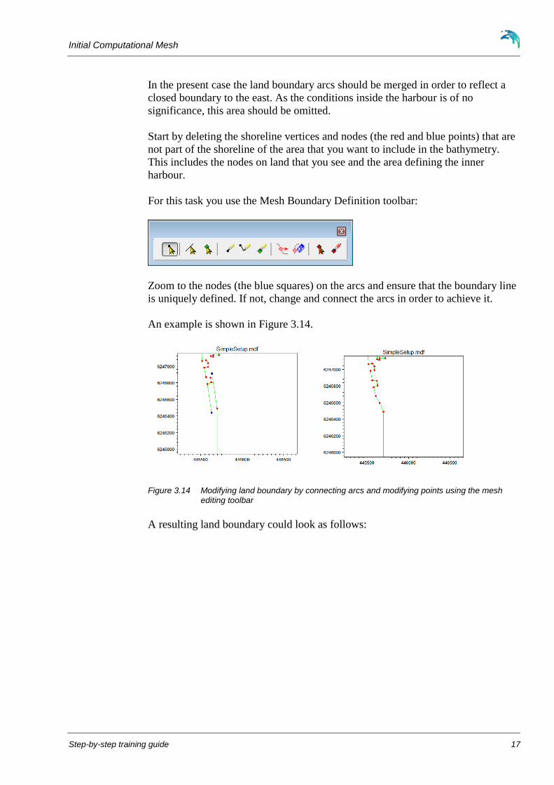
For this task you use the Mesh Boundary Definition toolbar:

Zoom to the nodes (the blue squares) on the arcs and ensure that the boundary line

is uniquely defined. If not, change and connect the arcs in order to achieve it.

An example is shown in Figure 3.14.

Figure 3.14 Modifying land boundary by connecting arcs and modifying points using the mesh

editing toolbar

A resulting land boundary could look as follows:

Mesh Generator

18 MIKE Zero

Figure 3.15 Resulting land boundary in the vicinity of the harbour

3.4.2 Adjusting the boundary data into a domain that can be triangulated

The domain area for the simulation is limited by the land boundary and three open

boundaries: a north, a west and a south boundary.

The domain area is selected to extend 10 km in the north-south direction and 4 km

in the east-west direction. This area is sufficiently large to avoid any influence of

the boundary settings in the vicinity of the harbour. Furthermore we do have

bathymetry information available to generate a good map.

Insert two nodes at the positions (442000, 6242000) and (442000, 6252000),

respectively. Note, that you can modify the location of a node afterwards by

selecting the node in the display, right-click Properties…

Connect the node points by drawing arcs to close the area. These new arcs define

the open boundaries. For aesthetic reasons you can move the land nodes on the

north and south boundary so the domain becomes nearly rectangular. This is

however not necessary.



The resulting domain may look as shown in Figure 3.16.

Figure 3.16 Defined domain area shown with background image and position of scatter data

3.5 Specification of Boundaries

The node points and arcs on the open boundaries must be defined by a unique

integer value. These attributes are used for the model system to distinguish

between the different boundary types in the mesh: attributes equal to 2 and above

correspond to open boundaries, attribute equal to 1 correspond to a land/water

boundary. Note that the attribute for a boundary will automatically be set to 1

during mesh generation if it is not already defined by a number larger than 1.

Mark the South Boundary arc, right-click and choose Properties. Set the arc and

node attributes to 2 for the southern boundary. Mark 3 for the western boundary

arc and mark 4 for the northern boundary arc, see Figure 3.17 and Figure 3.18.

Mesh Generator

20 MIKE Zero

Figure 3.17 Defined domain area shown with background image. Selecting the arc for the

northern boundary (purple arc) for editing properties (right click with mouse)

Figure 3.18 Editing the northern boundary arc properties



3.6 Mesh Generation

The next step is to triangulate the domain.

Try to make the first triangulation (MeshGenerate mesh…). Use the

triangulation option settings as shown in Figure 3.19.

Figure 3.19 The triangulation options for a first attempt

This setting will result in fewer than 500 elements. Elements limited by boundary

point positions tend to be much smaller than elements only limited by maximum

element area. The resulting mesh is shown in Figure 3.20.

Figure 3.20 Triangulated mesh for a first attempt

Mesh Generator

22 MIKE Zero

After the triangulation you can use a tool for smoothing the mesh (MeshSmooth

Mesh). In this example the mesh has been smoothed 100 times. The resulting

mesh will look as in Figure 3.21.

Figure 3.21 Resulting mesh after smoothing 100 times

We will consider how to refine the mesh in specific areas later in this step-by-step

guide.

3.7 Analysis

After mesh generation and smoothing of the mesh, it is feasible to analyse the

mesh in order to see if it can be improved. For this use the Analyse tool in the

toolbar (MeshAnalyse mesh…).

The simulation time for a setup increase with increasing number of elements,

decreasing element size and decreasing time step. The angles within the elements

should be as large as possible in order to optimize the solution. The analysis tool

can be applied to find individual elements that are limiting the optimal solution

setup.



Figure 3.22 Analyse mesh

The smaller the element, the smaller the time step must be to uphold the CFL

criteria. Thus isolated small elements should be avoided. In this case the land

boundary has been defined using two vertices positioned near each other. By

removing one of the vertices and regenerating the mesh, the smallest area value

will increase and so the time step required, see Figure 3.23.

Figure 3.23 Generated mesh after removing one vertex. The smallest element is now 7 times

larger

Mesh Generator

24 MIKE Zero

3.8 Smoothing the Mesh

In general, the mesh should be smoothed a number of times after the generation

and before interpolating the bathymetry. The smoothing process will change the

position of the generated node points in order to obtain the best overall resolution

of the triangular elements while trying to avoid small angles in too many elements.

In the examples shown in Figure 3.24 and Figure 3.25 a smoothing using 100

times will result in a smaller minimum element angle, but overall the element

angles are larger. Smoothing will only take place if the new mesh overall is better

than the original.

Figure 3.24 Generated mesh before smoothing. Note the 10 minimum angles found in analysis



Figure 3.25 Generated mesh after smoothing 100 times

Mesh Generator

26 MIKE Zero

Initial Bathymetry


4 INITIAL BATHYMETRY

The initial bathymetry is now created from the initial mesh by interpolating scatter

data.

4.1 Importing Scatter Data

First import the xyz-file containing the water depths from the measurements of

regional lines (DataManage Scatter Data Add… and choose the file

RegionalLines_1996.xyz). Specify the projection as UTM-32.

Figure 4.1 ASCII file describing the depth at specified geographical positions (Easting, Northing,

Depth (and point number). Please note that if MIKE C-MAP is used you are not allowed to view the data in a text editor because the data is encrypted. If C-MAP data is used then the co-ordinates will be given in Longitudes and Latitudes

Figure 4.2 Scatter data from regional lines

Mesh Generator

28 MIKE Zero

4.2 Interpolating Scatter Data

Now interpolate the bathymetry values by using the default settings for the

interpolation (MeshInterpolate…).

Figure 4.3 Interpolating water depths into the domain from imported XYZ file

Figure 4.4 The mesh as it appears in the Mesh Generator after interpolating water depth xyz

data into the mesh

Initial Bathymetry


4.3 Analysing the Mesh

After the interpolation of the bathymetry values, use the Mesh Analyse tool to

evaluate the mesh again, now investigating the element determining the smallest

time step, considering the water depth. This analysis may inspire to further

improvements of the mesh.

4.4 Exporting the Mesh

Now export the mesh from the Mesh Generator to a .mesh file.

4.5 Viewing the Mesh

You can view (and edit) the resulting mesh file in the Data Viewer (Figure 4.6) or

the Data Manager (Figure 4.7) or view it in Plot Composer or MIKE Animator

(Figure 4.8). Using the Animator is a very good tool to investigate the bathymetry

especially for spikes, strange ripples, decreasing depth just inside the boundary

etc.

The default editor/viewer for mesh/dfsu data files can be set to either the Data

Viewer or the Data Manager. You use the File Association dialog to choose the

default editor (Figure 4.5).

Figure 4.5 The File Association dialog

Please note that you may open the file with the alternative editor by right-clicking

the file in the Project Explorer and select ‘Open With’ instead of ‘Open’.

Mesh Generator

30 MIKE Zero

Figure 4.6 The interpolated mesh file as it appears in the Data Viewer. Left figure show the

bathymetry values (shown as smoothed contour), right figure show the node type values for the boundaries

Figure 4.7 The interpolated mesh file as it appears in the Data Manager. Bathymetry shown by

box contour

Initial Bathymetry


Figure 4.8 The interpolated mesh as it can be presented with the MIKE Animator tool

4.6 Next Steps

The initial domain describe an area of 4 km x 10 km, with bathymetry values from

-20 m up to + 6 m. The position of structures near the harbour (groins and

revetments) are outlined in the mesh.

The mesh generator setup for the initial resulting mesh is just a starting point for

optimizing the mesh to the final stage. In the following the initial mesh setup is

modified in a number of ways to achieve a better representation of the bathymetry

for the given simulation.

Mesh Generator

32 MIKE Zero

Mesh for Regional Wave Simulation


5 MESH FOR REGIONAL WAVE SIMULATION

Suppose the aim of the simulation is to investigate the overall wave conditions and

the transition of waves from deep water onto a position in front of the harbour

entrance.

In this case the details of the land contour is of less importance as the land contour

does not affect the wave conditions. Also, in order to evaluate the transformation

of the waves in detail, the number of elements in the deep area must be increased.

5.1 Modifying the Land Boundary

The elements near the land boundary depends highly on the resolution of the

boundary: for each vertex on the boundary line, a node will be generated. Thus by

modifying the number of vertices on the boundary line the mesh resolution will

change accordingly in the adjacent areas, cf. Figure 5.1 and Figure 5.2.

For example, if your line consist of many points, it may be feasible to re-distribute

the vertices on the line using a defined number of vertices or a defined distance.

This will smooth the boundary line and restrict the number of elements. Note that

the Preview button gives you the opportunity to preview the outline of the new

boundary before deciding to continue.

The overall wave conditions will not be affected by details near land, thus the land

contour can be modified to the simplest possible. In this case the groin tip can be

defined as a single node point and the coastline near the revetment can be

modified to a straight line.

Delete the generated mesh to modify the land boundary. The land boundary can be

edited by deleting the individual vertices on the arc.

Please note that removing the indication of the harbour would give even better

results. However in this instance the harbour is kept for educational purpose.

Mesh Generator

34 MIKE Zero

Figure 5.1 The land boundary. Left: initial boundary, right: after modifying

After modifying the land boundary, the mesh may be generated and smoothed in

order to see the effect of the changed setup. An example is shown in Figure 5.2.

Figure 5.2 Resulting mesh after modifying the land boundary



5.2 Increasing Resolution

In order to evaluate the wave transformation in the area, the mesh resolution must

be more refined.

5.2.1 Simple refinement of mesh

By refinement through bisection the existing mesh is used as basis for the

refinement. A number of face bisections determines how many times each element

is to be divided into 4 smaller elements, thus creating a more refined mesh. Note

that for each bisection, the total number of elements in the mesh is multiplied by a

factor of four.

An example of the mesh after refinement using bisection 1 time is shown in Figure

5.3.

Figure 5.3 Resulting mesh after refinement using bisection one time (1092 elements)

Please note that in this way it may still be the much smaller element areas near the

harbour entrance that will determine the simulation time.

Mesh Generator

36 MIKE Zero

5.2.2 Using smaller maximum element areas

A better way is to decrease the maximum element area used during the mesh

generation. By reducing the maximum element area by a factor of four, i.e. from

250000 to 62500, the mesh resolution in the deeper areas resembles the case using

bi-section but the creation of smaller areas near the harbour is avoided, thus

allowing for larger time steps in the simulation.

Figure 5.4 Resulting mesh after refinement using smaller maximum element area (966

elements)

5.3 Interpolating Bathymetry

The mesh resolution still seems a bit too coarse for the wave simulation, so in the

following a mesh with maximum element area 30000 m2 is applied, corresponding

to 2026 elements.

In the present case the focus is on the simulation of overall wave conditions. For

this the bathymetry information from the regional lines will contain the

information needed.



Figure 5.5 Importing of scatter data.

Figure 5.6 Resulting mesh with scatter data from regional lines (2026 elements)

After selecting the scatter data, interpolate the bathymetry using the default

settings.

Mesh Generator

38 MIKE Zero

Figure 5.7 Default settings in interpolation

The resulting bathymetry contains values from -20 to +10 m. The analysis show

that the maximum time step based on MWL=0m is around 3.7 s and that the

limiting elements are near the outer boundary where the water depth is the largest.



Figure 5.8 Resulting mesh bathymetry including applied scatter data

5.4 Refine Mesh in Shallow Areas

As the waves approach the shoreline the decreasing depth will cause the waves to

break. It is possible to refine the mesh, so the mesh elements in the shallower areas

decrease with the water depth. This process will not necessarily increase the

maximum time step as the outer elements will remain the same.

To refine by depth/gradient you have to have defined a zone before generating the

mesh.

Start over by deleting the generated mesh and insert a polygon marker in the

domain. Select the polygon marker and right-click to edit the polygon properties.

Per default the polygon will be excluded from the mesh, so change the properties

to ‘Apply triangular mesh’ and continue the usual way: generate the mesh, smooth

the mesh and interpolate the bathymetry.

Mesh Generator

40 MIKE Zero

Figure 5.9 Specifying polygon properties for main area

Once the mesh has been generated you can select to refine the mesh by depth or

gradient. Per default the relation is linear from the largest value to the smallest, but

it is possible to modify the ratio manually.

Figure 5.10 Specifying mesh refinement by depth ratio



In the example given the mesh refinement resulted in a mesh with 3699 elements,

while maintaining a maximum time step of 3.7 seconds in the Analysis.

Figure 5.11 Resulting mesh after refinement

5.5 Influence of Mesh Resolution on Simulation Results

To evaluate the effect of the size of the mesh elements on the results the MIKE 21

SW model has been setup for modelling a stationary wave with a height of 3 m

and coming from 300 degrees N. Three different meshes were applied in turn: the

initial mesh (shown in Figure 4.4), the detail SW mesh (shown in Figure 5.8) and

the refined detail SW mesh (shown in Figure 5.11).

The resulting wave fields are shown in Figure 5.12. It can be seen that the overall

wave transformation is the same, however the more refined the mesh, the more

details can be derived from the results. Thus, it is viable to use a mesh with large

mesh elements in areas that are not the subject of close investigation and use finer

elements in focus areas.

Note that the simulated wave conditions in the northern part of the area are not

similar to the rest, although this should be the case. The difference in the

conditions is due to the definition of the northern boundary, which shows the

importance of setting up a model where the focus area is well away from the

boundary.

Mesh Generator

42 MIKE Zero

Figure 5.12 Resulting wave field after wave simulation. Left: initial mesh, Middle: detailed mesh, Right: detailed mesh refined by depth ratio

Mesh for Local Wave Simulation


6 MESH FOR LOCAL WAVE SIMULATION

Suppose the aim of the simulation is to investigate the influence of the local

bathymetry on the wave conditions close to the harbour entrance.

In this case the details of the land contour and harbour structures is of importance

as to the accuracy of the bathymetry in the detail. Also, details in the bathymetry

should be resolved in order to evaluate the transformation of the waves in detail.

This entails both better scatter data and a more refined mesh in the area.

6.1 Available Data

The land boundary is digitized from map. Several scatter data sets are available,

both line surveys and surveys carried out in the harbour entrance.

An overview is given in Figure 6.1.

Figure 6.1 Available land and scatter data information. Conditions around the harbour entrance shown in detail to the right

Mesh Generator

44 MIKE Zero

6.2 Modifying the Land Boundary

The mesh generator setup for the initial resulting mesh is used as a starting point

for optimizing the mesh.

The land contours away from the harbour entrance can be simplified as this will

not affect the local wave conditions near the entrance. However, the land contours

representing the harbour from the first digitization were quite coarse.

One of the scatter data sets were derived by digitizing a survey map, created by

the local harbour authorities in 1996 (see Figure 6.2). This map contains details of

the harbour layout that can be used to improve the definition of the land contour in

the local area.

Figure 6.2 Bathymetric survey shown as background map to digitized land boundary

By moving and adding vertices to the land boundary it is possible to obtain a

better resolution of the harbour entrance as shown in Figure 6.3. When you are

satisfied with your modifications it may be a good idea to select the land boundary

line and export the arc to a xyz file for possible use later on.



Figure 6.3 Bathymetric survey shown as background map to edited land boundary

Note that the land boundary is defined with as few vertices as possible in order to

avoid small elements.

6.3 Using Polygons in Mesh Generation

In the area near the harbour the mesh resolution should be detailed, whereas the

deeper areas will do fine with a coarser mesh resolution. Apart from the general

refinement tools applied in the previous chapter, it is possible to control the mesh

resolution in certain areas by defining polygons where the local maximum element

area can be defined.

A polygon is an enclosed area surrounded by arcs. By adding a polygon marker

inside the polygon you may define the mesh resolution for the individual polygon.

The node point density within a polygon may be defined by selecting the polygon

marker; right click the indicated area and select Properties in the dropdown menu

(cf. Figure 6.4). This will open a dialog where you can define the type of the mesh

element (triangular/quadrangular) and the maximum element area within the

polygon (cf. Figure 6.5). Note that if you do not define a maximum element area

in this dialog, the maximum element area will be defined by the triangular mesh

element options in the Mesh Generation dialog.

Mesh Generator

46 MIKE Zero

Figure 6.4 Selection of polygon area to define properties

Figure 6.5 Definition of the properties of a defined polygon



The focus of the present simulation is on the area just outside the harbour, why the

mesh elements should be the smallest in this area. To ensure a smooth transition

between large elements in the deeper waters and small elements near the harbour,

a third polygon is defined as a transition area. The polygons can be defined to

follow the outline of the different scatter data sets as shown in Figure 6.6.

However, this is not necessary as the generation of the mesh and the interpolation

of the bathymetry are two separate processes.

Figure 6.6 Definition of polygons around harbour entrance

In this case the outer area is defined by overall settings with the maximum area set

to 30000 m2, the transition area is defined by a maximum element area of 5000 m

2

and the inner area is defined by a maximum element area of 1000 m2. Area wise

the scaling between different transitions areas should be in the range 4 to10 giving

a length scaling approximately between 2 and 3.

This gives a resulting mesh where the three polygon areas have distinctly different

mesh resolutions as shown to the left in Figure 6.7. Note that during the process of

smoothing the mesh elements there is an option to leave mesh nodes at arcs

untouched. Selecting this will mean that the internal arc defining the polygon will

be clearly seen in the resulting mesh. Thus, in this case the option should be

unchecked in order to get a smooth transition between the areas with different

resolution.

Mesh Generator

48 MIKE Zero

Figure 6.7 Generated mesh with using polygons (3219 elements).

Left: unsmoothed, Right: detail after smoothing

6.4 Prioritize Scatter Data

In the area near the harbour a number of different scatter data sets are available. It

is possible to add several data sets to the setup in mesh generator and then choose

to view and/or use only some of them in the mesh interpolation.

When adding several data sets to a setup some of the data may be obtained in the

same area. By just adding all data to the interpolation the data points are

considered equally valid and the resulting bathymetry will be derived as a mean of

the available data. However, often it would be preferred that some areas are

mostly affected by one particular data set. To enforce this prioritization,

prioritization areas can be included in the mesh generation, such that the weight of

each data set can be explicitly defined.

In the present example prioritization areas are defined to cover the areas with

overlaying data as shown in Figure 6.8. Note that the prioritization areas do not

have to correspond to the polygons used for the mesh generation.



Figure 6.8 Specification of prioritization area

Once the prioritization areas have been defined it is possible to prioritize the

scatter data in the different prioritization areas. This is done by defining different

weight combinations for the available scatter data sets and then apply one of the

defined weight combinations to the individual prioritization area as shown in

Figure 6.9.

Mesh Generator

50 MIKE Zero

Figure 6.9 Specification of prioritized scatter data in different areas

In this case, for example, the bathymetry in the harbour entrance is found by 95%

weight on the harbour survey and 5% weight on the local line survey. The regional

line survey data is not considered in this area.

Using this in the interpolation of the bathymetry (remember to enable ‘Use

prioritization’ in the dialog), it can be seen that the consistency of the depth

contours near the harbour entrance is better when the harbour survey is dominant

in the area than if all data sets has the same weight in the interpolation.



Figure 6.10 Resulting mesh bathymetry

Upper: including prioritization, Lower: excluding prioritization

6.5 Updating Mesh Bathymetry Using New Scatter Data

In case new scatter data must be considered it is not necessary to eliminate the

existing scatter data from the model setup. The change may be effectuated by

modifying the weight on the different scatter data sets, see Figure 6.11.

In this case a new harbour survey was conducted after a storm period, which

caused a bar to develop in front of the harbour entrance, see Figure 6.12.

Mesh Generator

52 MIKE Zero

Figure 6.11 Adding a new data set of scatter data. Display of old scatter data set is disabled

Figure 6.12 New harbour survey scatter data including survey image as background layer. Red lines indicate existing prioritization areas

A new mesh bathymetry is now to be generated based on this new harbour survey,

but keeping the existing line surveys. By modifying the weight combinations in

the existing prioritization areas or creating a new weight combination to apply in

the prioritization a new mesh bathymetry can be generated. Note that even if a

scatter data set is not displayed, it may still affect the interpolation.



Figure 6.13 Prioritization settings using new prioritization for harbour entrance

In the present setup the new scatter data set is the only one used in the

interpolation of the bathymetry within the harbour entrance prioritization area. The

resulting mesh bathymetry is shown in Figure 6.14.

Figure 6.14 Resulting mesh bathymetry using harbour survey from 1997 after a storm

Mesh Generator

54 MIKE Zero

6.6 Influence of Bathymetry on Simulation Results

To evaluate the influence of the different bathymetries the Spectral Wave Model is

rerun with the newly generated bathymetries. The result originating from the 1996

bathymetry is shown in Figure 6.15 and the result from the 1997 bathymetry is

shown in Figure 6.16.

Figure 6.15 Resulting wave field for 1996 survey

Figure 6.16 Resulting wave field for 1997 survey

From both surveys it can be seen that the presence of the bar in front of the

harbour has an influence on the wave field.

Likewise a MIKE 21 HD FM model is setup to simulate a current field created by

a constant water level gradient of 0.1 in the north-south direction. The results from

using the two different bathymetries is shown in Figure 6.17 and Figure 6.18.



Figure 6.17 Resulting flow field using the 1996 survey

Figure 6.18 Resulting flow field using the 1997 survey

It can be seen that the presence of the bar will cause the flow field downstream the

harbour entrance to diverge once the bar ends and the water depth increases.

Mesh Generator

56 MIKE Zero

Mesh for Longshore Current Simulation


7 MESH FOR LONGSHORE CURRENT SIMULATION

Suppose the aim of the simulation is to investigate the cross-shore distribution of

the wave properties and the longshore current profile, due to an incoming wave on

a nearly uniform coastline. In this case the wave and the current conditions would

be nearly constant in the longshore direction, but highly varying across the shore.

The details across the surf zone are very important and as such the mesh elements

must be sufficiently small to resolve the processes of the wave transformation. It

is, however, not necessary to have a fine resolution in the longshore direction as

the conditions will be nearly constant from one cross-section to the next.

Note that this type of condition is often similar to the requirements for modelling

river flow.

7.1 Defining Polygons for Customization

As the cross-shore section must be resolved with a high resolution in order to

describe the wave generated long shore current, the cross shore resolution should

normally cover the breaking zone with at least 5 to 10 elements cross shore. The

resulting mesh may end up containing very many elements by using the default

mesh generation with triangular elements as there is a limit on the minimum angle

in a triangular element. It is, however, possible instead to define the mesh by

quadrangular elements (or a combination of the two types). Using quadrangular

elements entails the possibility of having a fine resolution across the profile and a

coarser resolution along the coastline, thus reducing the total number of elements.

Please note that the elongated mesh elements will favour the flow direction along

the element. Hence, in case of divergence in the flow triangular elements will be a

better choice.

The overall domain area used in the initial mesh generator setup can be used as a

template, and the bathymetry values are derived from the regional lines.

The resulting mesh will be used to model south-westerly waves with focus on the

coastline north of the harbour entrance. Therefore, in order to define a finer mesh

resolution near the focus area, a number of polygons should be defined in order to

optimize the solution as shown in Figure 7.1.

As the details along the shoreline south of the harbour will not influence the wave

transformation and the longshore currents north of the harbour, the land boundary

is simplified in order to avoid unnecessary small elements.

Mesh Generator

58 MIKE Zero

Figure 7.1 Definition of polygon areas

As in the previous cases, the outer area should be to be defined by a triangular

mesh with a maximum area of 30000 m2. To ensure a smoother transition of the

longshore currents into the focus area, the southern polygon area will be defined

by a triangular mesh using a smaller maximum area, e.g. 5000 m2. The polygon

for the focus area will be defined by quadrangular elements.

7.1.1 Defining quadrangular elements

The necessary information for defining an area with quadrangular elements is

different from an area with triangular elements. For quadrangular elements, the

related polygon must be defined by at least 4 individual arcs. Two of these arcs are

selected to define the start and the end of the rectangular section, and these arcs

must not contain any vertices.

To define an area with quadrangular elements, right-click the polygon marker in

the display and press Properties… (cf. Figure 7.2).



Figure 7.2 Definition of quadrangular elements

First, select ‘Apply a quadrangular mesh’. This will enable the quadrangular mesh

options where you select the start arc and the end arc number. Note that these

numbers are found internally by the program and do not relate to the code value of

the arc.

Secondly, define the maximum length along the stream and transverse the stream

to e.g. 200 m and 25 m, respectively. This is a limit of the mesh element area,

similar to the value given for the maximum triangular area. Usually, the length

along the stream is larger than across. However there may be cases where it is

more feasible to define a stream in the ‘short’ direction.

Finally, press OK to save the definition of the quadrangular polygon area and

generate the mesh. During the generation of the mesh the quadrangular mesh

elements will be distributed uniformly within the associated polygon.

The resulting mesh could look as shown in Figure 7.3.

Mesh Generator

60 MIKE Zero

Figure 7.3 Resulting mesh (2943 elements). The figure to the right shows detail after smoothing

7.1.2 Interpolating bathymetry

The bathymetry values are to be based on the measured regional lines. These lines

are densely populated across the beach but carried out with some distance along

the beach, cf. Figure 7.4.

Figure 7.4 Scatter data from regional measuring lines



This kind of scatter data requires careful consideration with respect to the type of

interpolation. When interpolating scatter data in quadrangular element areas, there

are three types of interpolation methods as shown in Figure 7.5.

Figure 7.5 Definition of quadrangular interpolation options

The Natural neighbour and Linear options are similar to the options for the

triangular elements. The Inverse Distance Weighted option enables the optimal

use of scatter data where the points are not distributed uniformly in the area: by

setting a ‘strength’ value for the scatter data points in the longshore and cross-

shore direction respectively, it is possible to obtain a kind of prioritization of the

data in the interpolation process.

Mesh Generator

62 MIKE Zero

In the mesh shown in Figure 7.4, the resolution of the quadrangular grid is

sufficiently coarse to limit the influence of the choice of interpolation. However,

in case the resolution is fine and there are several mesh elements between the

measured lines, the choice of interpolation becomes important. This is the case if

the quadrangular element area is as detailed as shown in Figure 7.6.

Figure 7.6 Detailed quadrangular mesh area with measured regional scatter data lines



Figure 7.7 - Figure 7.10 shows the results of the different interpolation methods

for a part of the focus area when using the detailed mesh shown in Figure 7.6.

Please note that the depth contours in between the measured lines show

irregularities for linear and natural neighbour interpolation. By applying the

inverse distance method the default weight values gives unrealistic results, but by

applying a different weight factor for the x and y direction, respectively, the

expected symmetry of the natural bathymetry along the beach can be reproduced.

Figure 7.7 Interpolated bathymetry using linear interpolation

Figure 7.8 Interpolated bathymetry using natural neighbour interpolation

Mesh Generator

64 MIKE Zero

Figure 7.9 Interpolated bathymetry using Inverse distance weighted interpolation.

Strength value in flow direction: 2, and strength value transverse: 2

Figure 7.10 Interpolated bathymetry using Inverse distance weighted interpolation.

Strength value in flow direction: 2, and strength value transverse: 20

7.2 Neighbouring Quadrangular Element Areas

It is possible to generate a mesh with adjacent different quadrangular mesh

element areas when they share one of the definition arcs, i.e. are connected in the

longitudinal direction. In case the quadrangular elements areas cannot be defined

like this, it is necessary to generate a temporary mesh with a small band of

triangular elements to divide the two areas and then modify the mesh elements

manually to connect the quadrangular areas.



The example in Figure 7.11 shows how to create complex quadrangular mesh

areas: Assume that you south of the harbour entrance require 3 areas with

quadrangular elements to be located adjacent to each other. The mesh elements

within Area A must have a maximum length of 200 m and a width of 25 m (across

the beach). The mesh elements in Area B must have a maximum length of 200 m

and a maximum width of 100m. The mesh elements in Area C must have a

maximum length of 100 m.

Figure 7.11 Mesh Generator setup with 3 areas indicated for rectangular elements

7.2.1 Two adjacent areas

First define the polygons for Area A and Area B as shown in Figure 7.12 and

Figure 7.13.

Please note: It is only possible to connect two quadrangular polygon areas at the

start or end arc. Thus the maximum length transversal must be the same for the

two areas.

The resulting generated mesh is shown in Figure 7.14.

Mesh Generator

66 MIKE Zero

Figure 7.12 Polygon properties for Area A



Figure 7.13 Polygon properties for Area B

Mesh Generator

68 MIKE Zero

Figure 7.14 Resulting mesh in Area A and Area B



7.2.2 Complex combination of quadrangular areas

The next step is to define polygon properties for Area C. If this is done using the

entire area, the mesh generation process will halt issuing an error message.

Figure 7.15 Mesh generation result for illegal definition of polygon properties

To overcome this it is necessary to define additional node points such that Area C

is separated from Area A and Area B with a (narrow) section of triangular

elements, see Figure 7.17.

Note that the section with the triangular elements perform as a transition area

between the quadrangular sections.

In case the Area A, Area B and Area C is to be connected using only quadrangular

elements, it is necessary to control the mesh resolution in more detail. This can be

done by including vertices on the related boundary arcs. To get an estimate on the

number of vertices required, count the number of elements from the mesh in

Figure 7.17.

Mesh Generator

70 MIKE Zero

Figure 7.16 Polygon properties for Area C



Figure 7.17 Generated mesh using Area A, Area B and Area C.

Small section with triangular elements in transition area

Select the arcs enclosing the transition area and use the Arc Redistribution tool to

set the number of vertices to match the conditions from Area A and Area B, cf.

Figure 7.18. For more information on Arc Redistribution, please see section 8.1.1

on page76.

Figure 7.18 Redistribution of vertices along arcs to enable later transition to quadrangular

elements

Mesh Generator

72 MIKE Zero

Finally, divide the arc common with area C into two arcs that mirror the

conditions from Area A and Area B. This will allow for subsequent editing

towards quadrangular elements. To enforce an equal distribution of elements along

the north side of Area C, divide the arc into the same number of segments as on

the south side of Area C.

As the mesh element size is restricted along the polygon, define the maximum

length as the maximum length of an arc section at the boundary, e.g. 200 m, see

Figure 7.19.

Figure 7.19 Polygon properties for Area C, additional vertices to restrict element size



The generated mesh is shown in Figure 7.20. Having defined the transition area to

be narrow, it is a minor task to merge the triangular elements in the transition area

to quadrangular elements as shown in Figure 7.21. The resulting mesh is shown in

Figure 7.22.

Figure 7.20 Generated mesh using Area A, Area B and Area C.

Small section with triangular elements in transition area

Figure 7.21 Merging two triangular elements to one quadrangular element

Mesh Generator

74 MIKE Zero

Figure 7.22 Resulting mesh combining Area A, Area B and Area C with purely quadrangular

elements

The bathymetry for the resulting mesh can now be obtained by interpolation.

Please note that even if the resulting mesh file is saved in the .mdf file (showing

the manual editions), the edition will be lost if you regenerate the mesh.

Impact of Tidal Flow


8 IMPACT OF TIDAL FLOW

Another type of investigation could be the effect of the tidal water level variation

on the water level inside the harbour and associated flushing.

For a first attempt it is assumed that the gates at the entrance to the Thorsminde

bay is closed, why the large bay area is not included in the initial mesh.

The coastal outline for this simulation is to be based on the conditions after a

harbour extension. The data is extracted from MIKE C-MAP. The xyz files

exported from MIKE C-MAP are encrypted, so it is not possible to view the data

in a text editor. However, it is possible to import the data into the Mesh Generator.

Please note that all the data exported from MIKE C-MAP is stored in Long/Lat

values.

Figure 8.1 C-MAP data displayed in the Mesh Generator. Background image based on Google

Earth

Mesh Generator

76 MIKE Zero

8.1 Creating the Land Boundary

For this simulation the focus is on the inner harbour area. The layout of the inner

harbour is important as it has a direct impact on the water exchange. The details

near the shoreline, however, are not important.

The overall domain area used in the initial mesh generator setup can be used for a

template. To include the detailed land contour extracted from MIKE C-MAP,

import the land contour in file ‘land_CMAP_F.xyz’ that contains a detailed land

contour for the harbour area.

Please note that all the data exported from MIKE C-MAP is stored in Long/Lat

values.

Now modify the arcs to describe one land polyline that defines the shoreline and

the inner harbour area.

8.1.1 Redistribute vertices on arc

When digitizing land boundaries the number of vertices is often limited. When

importing land data from e.g. MIKE C-MAP the opposite may be the case; the

number of vertices on the arc lines may be very dense. As all vertices on a

boundary arc will result in a mesh node, this may result in very small elements in

the final mesh.

So far the boundary modifications in this step-by-step guide have mostly been

carried out by manually deleting and editing the vertices and node points.

However, it is possible to modify and re-arrange all the vertices along an arc

automatically, such that the resolution corresponds with the accuracy needed for

the mesh generation. Here, it is an advantage to use the Redistribute Vertices

option (cf. Figure 8.2 and Figure 8.3), which makes it possible to preview the

outcome of the changes (cf. Figure 8.4) before applying it to the mesh setup, as

opposed to the method of simply deleting the excess points. Since different

sections of the boundary line may need to be modified in different ways, it may be

feasible to divide the boundary line in separate arc sections by redefining a

number of vertices to node points.



Figure 8.2 Selection of arc in order to redistribute vertices

For long linear stretches it may be best to define the distance between the vertices.

With the help of the shown arc properties (cf. Figure 8.3), a constant distance

between the vertices may be suggested and only the nearest vertex will be

included in the new arc.

Mesh Generator

78 MIKE Zero

Figure 8.3 Arc redistribution. The initial properties of the selected arc is shown.

Figure 8.4 Arc redistribution. Before and after redistribution of vertices along the west side of the

inner harbour.

For arcs that are to be smoothed anyway it may be more feasible to define a fixed

number of vertices (cf. Figure 8.5). This way a new representative arc is created

based on a spline tension factor. Note that the vertices for the new arc are not

necessarily located on the existing arc. It is possible to preview the new resulting

arc before pressing OK to evaluate if the redistribution properties gives the

required result.



Figure 8.5 Arc redistribution. Preview of new arc at coastline using fixed number of vertices.

Usually the process of modifying a mesh boundary will consist of the combined

use of all the different ways of modifying arcs and points.

Note that the processes of modifying the boundary data may take some time. This

time, however, is saved later as the mesh will perform better in the simulation. It is

a good idea to save the mesh setup in different stages of the editing and in separate

files, in order to have the option to revert to an earlier stage of the editing.

The land boundary may look as shown in Figure 8.6 after some editing:

Please note that the land boundary will probably have to be edited even more after

the initial mesh generation as the analysis tool will point out elements that prevent

an optimal solution.

Mesh Generator

80 MIKE Zero

Figure 8.6 Land boundary after editing.

8.2 Specification of Domain

By assuming a constant water level variation in front of the harbour entrance due

to tide, the model area outside the harbour can be limited. Thus, the area in front

of the area is limited by one boundary line, onto which a constant time-varying

water level is to be defined in the simulation.

In order to gain details of the flow field inside the harbour an extra arc is defined

in order to define to polygons with individual mesh element settings, cf. Figure 8.7

and Figure 8.8.



Figure 8.7 Domain for simulation. Two polygons defines inner and outer area.

Figure 8.8 Generated mesh. The detailed mesh in the inner harbour (2784 elements)

Mesh Generator

82 MIKE Zero

8.3 Using Break Lines

When applying the scatter data it may occur that some of the scatter data should be

excluded from the interpolation, even if the scatter data is in adjacent areas. This is

the case of the inner harbour where the bathymetry data defining the coastal area

does not affect the depth of the harbour. In cases where the scatter data is divided

into separate files, e.g. one for the coastal area and one for the local harbour area,

it is possible to utilize the scatter data prioritization utility to explicitly define

which scatter data that is to be applied in the interpolation.

However, if all the scatter data is included in the same file, the interpolation will

try to use all the scatter data within the surroundings, even if the area is not

connected. In this case break lines can be applied when interpolating so that the

water depth in the harbour becomes independent of the water depth defining the

beach.

For this case assume that the depth in the harbour is constantly dredged to a

minimum depth of 5 m. To include this in the Mesh Generator setup, create a new

scatter data file containing the depth at a number of locations within the harbour.

In addition, add the scatter data for the local survey lines to describe the water

depths outside the harbour, cf. Figure 8.9.

Figure 8.9 Adding scatter data to new file

When just interpolating the scatter data it is seen that the scatter data from the

local lines from the sea will affect the water depths inside the harbour, see Figure

8.10. The effect can be minimized by reducing the extrapolation. This, however,

may affect other areas of the domain where a large extrapolation is needed.



Figure 8.10 Resulting bathymetry with standard interpolation

The solution is to create a break line that prevents the use of the un-wanted scatter

data points in the interpolation of the area. A break line is defined using an icon in

the Boundary Definition toolbar:

Figure 8.11 Inserting a break line from the Boundary Definition toolbar.

Note that you have to be in arc editing mode for the toolbar to activate

Define a line that divides the scatter data by the sea and the scatter data to be used

in the harbour area as shown in Figure 8.12. The interpolation will then only

consider the scatter data within the harbour area when calculating the depths in

here.

Mesh Generator

84 MIKE Zero

Figure 8.12 Definition of break line

Figure 8.13 Resulting bathymetry using break line

This bathymetry can now be used for simulating the flushing of the harbour during

tide. Please see Section 8.5 for results.



8.4 Increasing the Model Domain

The flow field through the harbour entrance for tidal simulations may change if

the water volume within the Thorsminde bay is added to the simulation.

For this particular simulation, the accuracy of the layout of the inner bay is of less

importance, as long as the overall area of the inner bay is correct.

The previous mesh generator setup can be used as a template.

Add the image of Jylland to the background and digitize the bay area by creating a

new arc. Attach the new arc to the existing setup and define the bay as a separate

polygon. Do also include the outline of the island in the southern part of the bay.

Mark this island as a polygon that is not to be a part of the mesh, cf. Figure 8.14.

After the mesh generation and interpolation the resulting mesh may look like the

one shown in Figure 8.15.

Figure 8.14 Adding inner bay to mesh setup. Background image based on Google Earth

Mesh Generator

86 MIKE Zero

Figure 8.15 Interpolated mesh including the inner bay. Bathymetry values are not edited

Please note that the bathymetry values in the inner bay near the outlet are based

on the scatter data in the harbour because of the break lines. However, the main

part of the bay is also influenced by the scatter data in the sea.

To overcome this, one can add more break lines to be included during the

interpolation. Sometimes, however, it is more convenient to modify the

bathymetry data after saving the mesh to a mesh file.

Open the saved mesh file in the Data Viewer and select the elements within the

bay area. Then set the overall bathymetry value to -5m, similar to the value in the

harbour area, cf. Figure 8.16.



Figure 8.16 Modification of bathymetry values using the Data Viewer

Figure 8.17 Detail of resulting mesh bathymetry after modification

Mesh Generator

88 MIKE Zero

8.5 Simulation Results

To evaluate the effect that the tide and the additional bay area have on the flow in

the harbour area, different model setups are simulated. Some results are shown in

Figure 8.18 - Figure 8.22.

Note that the flow field is very dependent on whether the gate is open or not.

Figure 8.18 Detail of resulting flow field in harbour when gates are closed

Figure 8.19 Detail of resulting flow field and surface elevation in harbour when gates are closed at

high tide



Figure 8.20 Detail of resulting flow field and surface elevation when gates are open at high tide

Figure 8.21 Resulting surface elevation in the domain when gates are open at high tide

Figure 8.22 Extract of surface elevation 100 m on each side of the gate

Mesh Generator

90 MIKE Zero

Phase II of Previous Investigation


9 PHASE II OF PREVIOUS INVESTIGATION

It happens that model setups used in older investigations may be needed again

because the boundary conditions have changed, e.g. a new harbour layout is being

made. This will often cause an investigation as to how the changed layout will

affect the flow pattern. Preferably this investigation would be carried out before

any constructions take place, but sometimes the investigations are carried out

because something un-expected has happened.

In some cases the original .mdf file has been saved. Then the modifications to a

new layout is fairly simple, - just modify the settings with the new information and

re-generate the mesh.

In case it is only the bathymetry data that has changed, e.g. due to a new harbour

survey, it is sufficient to import the mesh directly into a new .mdf file and then re-

interpolate the bathymetry using the new values.

However, sometimes the only available data is the existing mesh file and the

information about the new land boundary and possible changes in the bathymetry.

In that case, the generation of a new mesh requires more work using manual pre-

processing of the data. Such a case is described in the following.

Consider the case with the existing mesh bathymetry as displayed in Figure 9.1.

Figure 9.1 Existing mesh bathymetry

Mesh Generator

92 MIKE Zero

The bathymetry contains 4211 nodes and 7876 elements, with smaller elements

defining the area around the harbour entrance.

After some years a new layout of the harbour entrance has been defined. Now it is

necessary to update the existing mesh with the new information to simulate the

changes caused by the new layout.

The information regarding the new harbour layout is derived from extracting land

boundary data from MIKE C-MAP. The outline of the changes needed is indicated

in Figure 9.2. This is similar to the data displayed in Figure 8.1.

Obviously the bathymetry values will have changed after the construction, but this

is not considered in the present exercise.

Figure 9.2 Existing mesh bathymetry.

Outline of new land boundary is indicated by xyz point display



9.1 Modifying Existing Mesh File

If the number of changes to the mesh are minor, it may be most practical to just

modify the existing mesh directly by using the Mesh Editing facilities, manually.

Create a new mesh generator setup by loading in the existing mesh directly using

the Load mesh command. Next import the Land boundary as scatter data as shown

in Figure 9.4. The scatter data will be used as a guide line for the modifications.

The task ahead is now to modify the mesh to match the new layout and then

interpolate the bathymetry using the bathymetry values from the existing mesh.

The Mesh Editing toolbar shown in Figure 9.3 contains a number of different tools

that can be used for this purpose.

Figure 9.3 Mesh Editing toolbar

9.1.1 Moving mesh nodes

Try to move the node points to a position such that the outline of the new

structures is shown, cf. Figure 9.4.

Figure 9.4 Moving mesh nodes in existing mesh bathymetry. Land scatter data shown as points

Mesh Generator

94 MIKE Zero

Note that this may cause some of the areas or the angles in some of the triangles to

become very small. In order to analyse the changes use the Analyse tool to

identify areas where the mesh modification could be improved, cf. Figure 9.5.

Figure 9.5 Example of analysis of modified mesh. Upper: Analysis result before editing problematic mesh element. Lower: Analysis result after editing

However, it may be easier to re-triangulate the affected area.



9.1.2 Re-triangulate selected region

Moving mesh nodes will often give rise to mesh elements that are small or have

small angles. In order to optimize the mesh after the changes it is possible to re-

triangulate the mesh elements in a selected area, cf. Figure 9.6. This will leave the

mesh nodes outside the selected area untouched.

Figure 9.6 Re-triangulation of selected region.

Upper: selected area to re-triangulate Lower: resulting new mesh after re-triangulation using maximum area of 100

Keep the land inside the triangulation area. This will ensure that the boundary

node points will keep the original position.

Note that re-triangulation can be used as a way to increase the number of mesh

node points in a certain area before a manual adaption of the mesh begins.

Mesh Generator

96 MIKE Zero

9.1.3 Adding node points

In some areas the moved points may cause single mesh elements to be quite large.

Apart from the option to re-triangulate a selected region, it is also possible to

improve the mesh resolution by adding an extra mesh node into the mesh element

as shown in Figure 9.7. You have the option to re-triangulate the adjacent

elements as well. In most cases this will be feasible as the overall mesh layout will

be better, but in some cases it is better to maintain the layout of the adjacent mesh

elements, cf. Figure 9.8.

Figure 9.7 Adding a mesh node

Figure 9.8 Resulting mesh after adding mesh node. Left: including re-triangulation of adjacent elements, Right: no re-triangulation

Similarly, it is possible to add a node point to a boundary. In this case only the

affected element is modified.



9.1.4 Deleting mesh nodes

Try to delete the mesh nodes that are located in areas where new the new structure

should be. When asked for method, select ‘Make land’, cf. Figure 9.9. This will

reduce the number of mesh elements and it will be easier to move the remaining

mesh nodes to a position to outline the new structure. Figure 9.10 shows a

resulting mesh after deleting and moving mesh nodes.

Figure 9.9 Deleting mesh nodes from existing mesh bathymetry

Figure 9.10 Resulting mesh after deleting and moving mesh nodes

Once the new boundary has been updated to a satisfactory level, the mesh can be

optimized by using re-triangulation for a selected area.

Mesh Generator

98 MIKE Zero

9.1.5 Interpolating bathymetry

The node points already contain bathymetry information from the original mesh.

However, as the points have moved around, and additional points have been

added, it is necessary to interpolate the bathymetry values in the new mesh.

Add the original mesh as scatter data points using either the generated xyz-file

with the original node points or the .mesh file itself. The display of scatter data

shows where the new mesh match the old, cf. Figure 9.11.

Figure 9.11 Scatter data from existing mesh displayed on new mesh

The resulting mesh have the same values in the node points that are not moved,

whereas new and modified points will have bathymetry values interpolated from

the original mesh as shown in Figure 9.12.



Figure 9.12 Detail of resulting bathymetry after modification and interpolation

9.1.6 Modifying properties of single mesh node

Note that the bathymetry in the southern part of the harbour entrance area has been

interpolated based on the sediment accumulated south of the old structure. It is

possible to modify the bathymetry values in several ways. A simple way is to

modify the bathymetry in individual mesh nodes in the resulting mesh using the

Data Viewer, but it is also possible to modify the mesh node properties for an

individual node in the Mesh Generator by using the Edit mesh node option tool in

the Mesh Editing toolbar as shown in Figure 9.13.

Figure 9.13 Mesh node editing using the Mesh Editing toolbar

Mesh Generator

100 MIKE Zero

9.1.7 Evaluating change

It is possible to see the changes in the bathymetry by subtracting the two files

using the calculator in Data Manager. The resulting difference may be as shown in

Figure 9.14.

Figure 9.14 Difference in bathymetry values before and after modification.

Note, the difference values near the land boundary lines are due to interpolation issues in the difference calculations

9.2 Re-establishing .mdf File for Existing Mesh

In case the number of changes to the mesh bathymetry is anticipated to be a major

task, it may be less time consuming in the long run to re-establish (most of) the

.mdf file used for creation of the existing mesh and then apply the changes using

the Arc Editing facilities.

Create a new mesh generator setup by loading the existing mesh directly using the

Load mesh command. The outlined mesh elements will be useful as a background

layer when creating the new setup.



Figure 9.15 Outline of existing mesh bathymetry

Change the settings from ‘Mesh Editing’ to ‘Arc Editing’ and save the mesh

generator setup. The workspace and map projection have now been defined and it

is possible to progress with re-establishing the mesh.

9.2.1 Extract node point data from mesh

In order to re-generate the existing mesh accurately, it is necessary to define all the

node points in the existing positions in the mesh generator setup.

The mesh node section of the mesh file contains the xyz information of all the

nodes (see Section 1.6). It is thus possible to extract this information and save the

data in an ascii file with extension xyz, e.g. using EXCEL. The file can then be

imported as scatter data in a new mesh generator setup.

Mesh Generator

102 MIKE Zero

9.2.2 Import node points

Use the Manage Scatter Data dialog to import the node point scatter data

previously extracted from the existing mesh file.

Figure 9.16 Imported scatter data based on mesh node points

These points can now be converted to mesh nodes by using the Convert button in

the Manage Scatter Data dialog as shown in Figure 9.17.

All the scatter data will now be converted into node points. As node points are

fixed locations, a mesh similar to the original existing mesh will automatically be

created during the mesh generation process if it is purely triangular elements. In

case of quadrangular elements in the original mesh, the new mesh will contain two

triangles for each quadrangle.



Figure 9.17 Converting scatter data to node points

Figure 9.18 Existing node points derived from scatter data

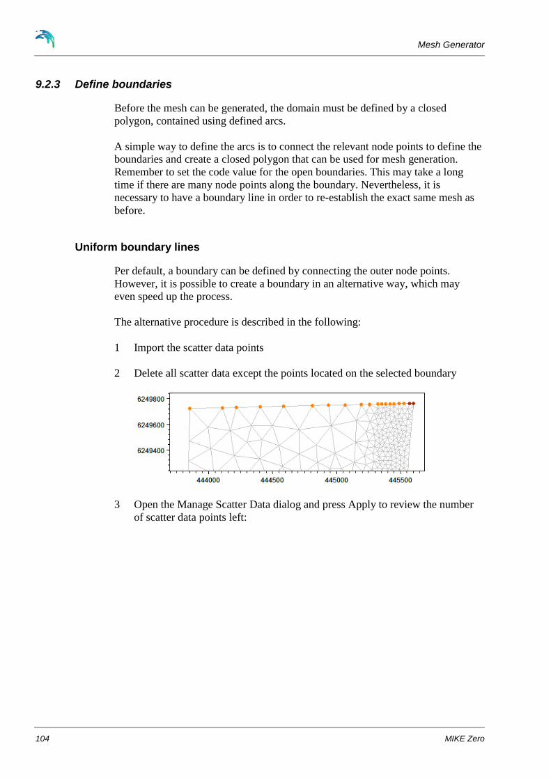
Mesh Generator

104 MIKE Zero

9.2.3 Define boundaries

Before the mesh can be generated, the domain must be defined by a closed

polygon, contained using defined arcs.

A simple way to define the arcs is to connect the relevant node points to define the

boundaries and create a closed polygon that can be used for mesh generation.

Remember to set the code value for the open boundaries. This may take a long

time if there are many node points along the boundary. Nevertheless, it is

necessary to have a boundary line in order to re-establish the exact same mesh as

before.

Uniform boundary lines

Per default, a boundary can be defined by connecting the outer node points.

However, it is possible to create a boundary in an alternative way, which may

even speed up the process.

The alternative procedure is described in the following:

1 Import the scatter data points

2 Delete all scatter data except the points located on the selected boundary

3 Open the Manage Scatter Data dialog and press Apply to review the number

of scatter data points left:



4 Press Reduce data and specify a new output xyz file name to contain the

remaining scatter data points. Define a small distance threshold in order to

save all points:

When clicking the Reduce button, the program will save the scatter data

points in the new xyz file in a sequence ordered according to increasing x-

position for the points.

Mesh Generator

106 MIKE Zero

5 Now, include the xyz-data file as a boundary in the mesh generator setup.

Select the column sequence as the last option and define the arc as ‘Add all

vertices to one arc’:



This will import the selected data as one boundary line:

Please note that when importing the boundaries from xyz-files, the node points at

the boundary from the converted scatter data should be deleted in order not to

have duplicate points in the mesh generation.

Complex boundary lines

In case the node points at the boundary are not connected in a simple way it is

necessary to divide the boundary into smaller sections that each are uniformly

directed if the boundary is to be imported from xyz-files. Otherwise, it is

necessary to connect the points manually. Note that it may ease the subsequent arc

editing if some of the connected node points are transformed to vertices thus

creating one arc instead of a group of individual arcs.

Figure 9.19 Manual creation of arc

Mesh Generator

108 MIKE Zero

9.2.4 Create mesh

After having closed the domain with arcs, generate the mesh. As the node points

are fixed locations in the mesh generation process, a mesh similar to the original

existing mesh will automatically be created.

9.2.5 Interpolate mesh

Next, import the scatter data points or alternatively the original mesh as scatter

data and interpolate the mesh. In this case the interpolation option ‘Set value from

scatter data’ will make a quick interpolation finding the exact same bathymetry

values as in the original mesh.

The resulting mesh will be a replica of the original mesh, cf. Figure 9.20. You can

now use the generated .mdf file to make further modifications to the mesh as

described in the previous sections.

Figure 9.20 Resulting mesh bathymetry. Upper: new mesh, Lower: original mesh

MIKE ZERO Mesh Generator Step-by-step training...

Documents

Transcript of MIKE ZERO Mesh Generator Step-by-step training...