MIKE 21 and MIKE 3 Flow Model FM Hydrodynamic Module · realistic representations of nature, both...
14
MIKE 21 & MIKE 3 Flow Model FM Hydrodynamic Module Short Description
Transcript of MIKE 21 and MIKE 3 Flow Model FM Hydrodynamic Module · realistic representations of nature, both...

MIKE 21 & MIKE 3 Flow Model FM
Hydrodynamic Module
Short Description

© DHI
DHI headquarters
Agern Allé 5
DK-2970 Hørsholm
Denmark
+45 4516 9200 Telephone
+45 4516 9333 Support
+45 4516 9292 Telefax
www.mikepoweredbydhi.com
MIK
E2
13
_H
D_
FM
_S
hort
_D
escri
ption
_.d
ocx /
AJS
/EB
R/N
HP
/ 2
01
7-1
0-0
2

The Modules of the Flexible Mesh Series
1
MIKE 21 & MIKE 3 Flow Model FM
The Flow Model FM is a comprehensive modelling
system for two- and three-dimensional water
modelling developed by DHI. The 2D and 3D models
carry the same names as the classic DHI model
versions MIKE 21 & MIKE 3 with an ‘FM’ added
referring to the type of model grid - Flexible Mesh.
The modelling system has been developed for
complex applications within oceanographic, coastal
and estuarine environments. However, being a
general modelling system for 2D and 3D free-
surface flows it may also be applied for studies of
inland surface waters, e.g. overland flooding and
lakes or reservoirs.
MIKE 21 & MIKE 3 Flow Model FM is a general hydrodynamic flow modelling system based on a finite volume method on an unstructured mesh
The Modules of the Flexible Mesh Series DHI’s Flexible Mesh (FM) series includes the
following modules:
Flow Model FM modules
Hydrodynamic Module, HD
Transport Module, TR
Ecology Modules, MIKE ECO Lab/AMB Lab
Oil Spill Module, OS
Mud Transport Module, MT
Particle Tracking Module, PT
Sand Transport Module, ST
Shoreline Morphology Module, SM
Wave module
Spectral Wave Module, SW
The FM Series meets the increasing demand for
realistic representations of nature, both with regard
to ‘look alike’ and to its capability to model coupled
processes, e.g. coupling between currents, waves
and sediments. Coupling of modules is managed in
the Coupled Model FM.
All modules are supported by advanced user
interfaces including efficient and sophisticated tools
for mesh generation, data management, 2D/3D
visualization, etc. In combination with
comprehensive documentation and support, the FM
series forms a unique professional software tool for
consultancy services related to design, operation
and maintenance tasks within the marine
environment.
An unstructured grid provides an optimal degree of
flexibility in the representation of complex
geometries and enables smooth representations of
boundaries. Small elements may be used in areas
where more detail is desired, and larger elements
used where less detail is needed, optimising
information for a given amount of computational
time.
The spatial discretisation of the governing equations
is performed using a cell-centred finite volume
method. In the horizontal plane, an unstructured grid
is used while a structured mesh is used in the
vertical domain (3D).
This document provides a short description of the
Hydrodynamic Module included in MIKE 21 & MIKE
3 Flow Model FM.
Example of computational mesh for Tamar Estuary, UK

MIKE 21 & MIKE 3 Flow Model FM
2 Hydrodynamic Module - © DHI
MIKE 21 & MIKE 3 Flow Model FM - Hydrodynamic Module
The Hydrodynamic Module provides the basis for
computations performed in many other modules, but
can also be used alone. It simulates the water level
variations and flows in response to a variety of
forcing functions on flood plains, in lakes, estuaries
and coastal areas.
Application Areas The Hydrodynamic Module included in MIKE 21 &
MIKE 3 Flow Model FM simulates unsteady flow
taking into account density variations, bathymetry
and external forcings.
The choice between 2D and 3D model depends on a
number of factors. For example, in shallow waters,
wind and tidal current are often sufficient to keep the
water column well-mixed, i.e. homogeneous in
salinity and temperature. In such cases a 2D model
can be used. In water bodies with stratification,
either by density or by species (ecology), a 3D
model should be used. This is also the case for
enclosed or semi-enclosed waters where wind-
driven circulation occurs.
Typical application areas are
Assessment of hydrographic conditions for
design, construction and operation of structures
and plants in stratified and non-stratified waters
Environmental impact assessment studies
Coastal and oceanographic circulation studies
Optimization of port and coastal protection
infrastructures
Lake and reservoir hydrodynamics
Cooling water, recirculation and desalination
Coastal flooding and storm surge
Inland flooding and overland flow modelling
Forecast and warning systems
Example of a global tide application of MIKE 21 Flow Model FM. Results from such a model can be used as boundary conditions for regional scale forecast or hindcast models
MIKE 21 & MIKE 3 FLOW MODEL FM supports both Cartesian and spherical coordinates. Spherical coordinates are usually applied for regional and global sea circulation applications. The chart shows the computational mesh and bathymetry for the planet Earth generated by the MIKE Zero Mesh Generator
Application Areas
3
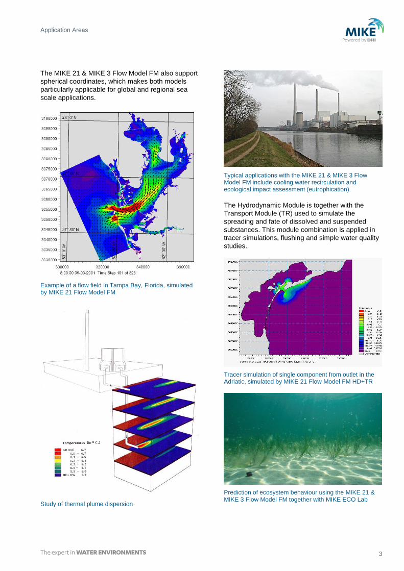
The MIKE 21 & MIKE 3 Flow Model FM also support
spherical coordinates, which makes both models
particularly applicable for global and regional sea
scale applications.
Example of a flow field in Tampa Bay, Florida, simulated by MIKE 21 Flow Model FM
Study of thermal plume dispersion
Typical applications with the MIKE 21 & MIKE 3 Flow Model FM include cooling water recirculation and ecological impact assessment (eutrophication)
The Hydrodynamic Module is together with the
Transport Module (TR) used to simulate the
spreading and fate of dissolved and suspended
substances. This module combination is applied in
tracer simulations, flushing and simple water quality
studies.
Tracer simulation of single component from outlet in the Adriatic, simulated by MIKE 21 Flow Model FM HD+TR
Prediction of ecosystem behaviour using the MIKE 21 & MIKE 3 Flow Model FM together with MIKE ECO Lab

MIKE 21 & MIKE 3 Flow Model FM
4 Hydrodynamic Module - © DHI
The Hydrodynamic Module can be coupled to the
Ecological Module (MIKE ECO Lab) to form the
basis for environmental water quality studies
comprising multiple components.
Furthermore, the Hydrodynamic Module can be
coupled to sediment models for the calculation of
sediment transport. The Sand Transport Module and
Mud Transport Module can be applied to simulate
transport of non-cohesive and cohesive sediments,
respectively.
In the coastal zone the transport is mainly
determined by wave conditions and associated
wave-induced currents. The wave-induced currents
are generated by the gradients in radiation stresses
that occur in the surf zone. The Spectral Wave
Module can be used to calculate the wave conditions
and associated radiation stresses.
Model bathymetry of Taravao Bay, Tahiti
Coastal application (morphology) with coupled MIKE 21 HD, SW and ST, Torsminde harbour Denmark
Example of vertical profile of cross reef currents in Taravao Bay, Tahiti simulated with MIKE 3 Flow Model FM. The circulation and renewal of water inside the reef is dependent on the tides, the meteorological conditions and the cross reef currents, thus the circulation model includes the effects of wave induced cross reef currents

Computational Features
5
Computational Features The main features and effects included in
simulations with the MIKE 21 & MIKE 3 Flow Model
FM – Hydrodynamic Module are the following:
Flooding and drying
Momentum dispersion
Bottom shear stress
Coriolis force
Wind shear stress
Barometric pressure gradients
Ice coverage
Tidal potential
Precipitation/evaporation
Infiltration
Heat exchange with atmosphere
Wave radiation stresses
Sources and sinks, incl. jet
Structures
Model Equations The modelling system is based on the numerical
solution of the two/three-dimensional incompressible
Reynolds averaged Navier-Stokes equations subject
to the assumptions of Boussinesq and of hydrostatic
pressure. Thus, the model consists of continuity,
momentum, temperature, salinity and density
equations and it is closed by a turbulent closure
scheme. The density does not depend on the
pressure, but only on the temperature and the
salinity.
For the 3D model, the free surface is taken into
account using a sigma-coordinate transformation
approach or using a combination of a sigma and z-
level coordinate system.
Below the governing equations are presented using
Cartesian coordinates.
The local continuity equation is written as
Sz
w
y
v
x
u
and the two horizontal momentum equations for the
x- and y-component, respectively
Suz
u
zFdz
x
g
x
p
xgfv
z
wu
y
vu
x
u
t
u
stuz
a
00
2
1
Svz
v
zFdz
y
g
y
p
ygfu
z
wv
x
uv
y
v
t
v
stvz
a
00
2
1
Temperature and salinity In the Hydrodynamic Module, calculations of the
transports of temperature, T, and salinity, s follow
the general transport-diffusion equations as
STHz
TD
zF
z
wT
y
vT
x
uT
t
TsvT
Ssz
sD
zF
z
ws
y
vs
x
us
t
ssvs
Unstructured mesh technique gives the maximum degree of flexibility, for example: 1) Control of node distribution allows for optimal usage of nodes 2) Adoption of mesh resolution to the relevant physical scales 3) Depth-adaptive and boundary-fitted mesh. Below is shown an example from Ho Bay, Denmark with the approach channel to the Port of Esbjerg

MIKE 21 & MIKE 3 Flow Model FM
6 Hydrodynamic Module - © DHI
The horizontal diffusion terms are defined by
sTy
Dyx
Dx
FF hhsT ,,
The equations for two-dimensional flow are obtained
by integration of the equations over depth.
Heat exchange with the atmosphere is also included.
Symbol list
t time
x, y, z Cartesian coordinates
u, v, w flow velocity components
T, s temperature and salinity
Dv vertical turbulent (eddy) diffusion
coefficient
Ĥ source term due to heat exchange with
atmosphere
S magnitude of discharge due to point
sources
Ts, ss temperature and salinity of source
FT, Fs, Fc horizontal diffusion terms
Dh horizontal diffusion coefficient
h depth
Solution Technique The spatial discretisation of the primitive equations is
performed using a cell-centred finite volume method.
The spatial domain is discretised by subdivision of
the continuum into non-overlapping elements/cells.
Principle of 3D mesh
In the horizontal plane an unstructured mesh is used
while a structured mesh is used in the vertical
domain of the 3D model. In the 2D model the
elements can be triangles or quadrilateral elements.
In the 3D model the elements can be prisms or
bricks whose horizontal faces are triangles and
quadrilateral elements, respectively.
The effect of a number of structure types (weirs,
culverts, dikes, gates, piers and turbines) with a
horizontal dimension which usually cannot be
resolved by the computational mesh is modelled by
a subgrid technique.
Model Input Input data can be divided into the following groups:
Domain and time parameters:
- computational mesh (the coordinate type is
defined in the computational mesh file) and
bathymetry
- simulation length and overall time step
Calibration factors
- bed resistance
- momentum dispersion coefficients
- wind friction factors
- heat exchange coefficients
Initial conditions
- water surface level
- velocity components
- temperature and salinity
Boundary conditions
- closed
- water level
- discharge
- temperature and salinity
Other driving forces
- wind speed and direction
- tide
- source/sink discharge
- wave radiation stresses
Structures
- Structure type
- location
- structure data

Model Input
7
Setup definition of culvert structure
View button on all the GUIs in MIKE 21 & MIKE 3 FM HD for graphical view of input and output files
Providing MIKE 21 & MIKE 3 Flow Model FM with a
suitable mesh is essential for obtaining reliable
results from the models. Setting up the mesh
includes the appropriate selection of the area to be
modelled, adequate resolution of the bathymetry,
flow, wind and wave fields under consideration and
definition of codes for defining boundaries.
The Mesh Generator is an efficient MIKE Zero tool for the generation and handling of unstructured meshes, including the definition and editing of boundaries
2D visualization of a computational mesh (Odense Estuary)
Bathymetric values for the mesh generation can e.g.
be obtained from the MIKE Powered by DHI product
MIKE C-Map. MIKE C-Map is an efficient tool for
extracting depth data and predicted tidal elevation
from the world-wide Electronic Chart Database CM-
93 Edition 3.0 from C-MAP Norway.

MIKE 21 & MIKE 3 Flow Model FM
8 Hydrodynamic Module - © DHI
3D visualization of a computational mesh
If wind data is not available from an atmospheric
meteorological model, the wind fields (e.g. cyclones)
can be determined by using the wind-generating
programs available in MIKE 21 Toolbox.
Global winds (pressure & wind data) can be
downloaded for immediate use in your simulation.
The sources of data are from GFS courtesy of
NCEP, NOAA. By specifying the location, orientation
and grid dimensions, the data is returned to you in
the correct format as a spatial varying grid series or
a time series. The link is:
http://www.waterforecast.com/hindcastdataproducts
The chart shows a hindcast wind field over the North Sea and Baltic Sea as wind speed and wind direction
Model Output Computed output results at each mesh element and
for each time step consist of:
Basic variables
- water depths and surface elevations
- flux densities in main directions
- velocities in main directions
- densities, temperatures and salinities
Additional variables
- Current speed and direction
- Wind velocity
- Air pressure
- Drag coefficient
- Precipitation/evaporation
- Courant/CFL number
- Eddy viscosity
- Element area/volume
The output results can be saved in defined points,
lines and areas. In the case of 3D calculations, the
results are saved in a selection of layers.
Output from MIKE 21 & MIKE 3 Flow Model FM is
typically post-processed using the Data Viewer
available in the common MIKE Zero shell. The Data
Viewer is a tool for analysis and visualization of
unstructured data, e.g. to view meshes, spectra,
bathymetries, results files of different format with
graphical extraction of time series and line series
from plan view and import of graphical overlays.
The Data Viewer in MIKE Zero – an efficient tool for analysis and visualization of unstructured data including processing of animations. Above screen dump shows surface elevations from a model setup covering Port of Copenhagen
Vector and contour plot of current speed at a vertical profile defined along a line in Data Viewer in MIKE Zero
Validation
9
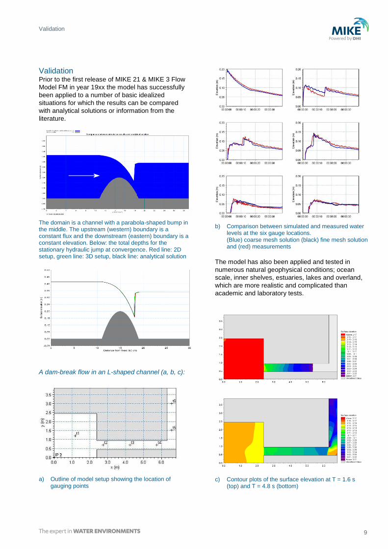
Validation Prior to the first release of MIKE 21 & MIKE 3 Flow
Model FM in year 19xx the model has successfully
been applied to a number of basic idealized
situations for which the results can be compared
with analytical solutions or information from the
literature.
The domain is a channel with a parabola-shaped bump in the middle. The upstream (western) boundary is a constant flux and the downstream (eastern) boundary is a constant elevation. Below: the total depths for the stationary hydraulic jump at convergence. Red line: 2D setup, green line: 3D setup, black line: analytical solution
A dam-break flow in an L-shaped channel (a, b, c):
a) Outline of model setup showing the location of gauging points
b) Comparison between simulated and measured water levels at the six gauge locations. (Blue) coarse mesh solution (black) fine mesh solution and (red) measurements
The model has also been applied and tested in
numerous natural geophysical conditions; ocean
scale, inner shelves, estuaries, lakes and overland,
which are more realistic and complicated than
academic and laboratory tests.
c) Contour plots of the surface elevation at T = 1.6 s (top) and T = 4.8 s (bottom)

MIKE 21 & MIKE 3 Flow Model FM
10 Hydrodynamic Module - © DHI
Example from Ho Bay, a tidal estuary (barrier island coast) in South-West Denmark with access channel to the Port of Esbjerg.
Comparison between measured and simulated water levels
The user interface of the MIKE 21 and MIKE 3 Flow Model FM (Hydrodynamic Module), including an example of the extensive Online Help system

Graphical User Interface
11
Graphical User Interface The MIKE 21 & MIKE 3 Flow Model FM
Hydrodynamic Module is operated through a fully
Windows integrated graphical user interface (GUI).
Support is provided at each stage by an Online Help
system.
The common MIKE Zero shell provides entries for
common data file editors, plotting facilities and
utilities such as the Mesh Generator and Data
Viewer.
Overview of the common MIKE Zero utilities
Parallelisation The computational engines of the MIKE 21 & MIKE 3
FM series are available in versions that have been
parallelised using both shared memory as well as
distributed memory architecture. The latter approach
allows for domain decomposition. The result is much
faster simulations on systems with multiple cores. It
is also possible to use a graphics card (GPU) to
perform computational intensive hydrodynamic
computations.
Example of MIKE 21 HD FM speed-up using a HPC Cluster with distributed memory architecture (purple)
Hardware and Operating System Requirements The MIKE Zero Modules support Microsoft Windows
7 Professional Service Pack 1 (64 bit), Windows 10
Pro (64 bit), Windows Server 2012 R2 Standard (64
bit) and Windows Server 2016 Standard (64 bit).
Microsoft Internet Explorer 9.0 (or higher) is required
for network license management. An internet
browser is also required for accessing the web-
based documentation and online help.
The recommended minimum hardware requirements
for executing the MIKE Zero modules are:
Processor: 3 GHz PC (or higher)
Memory (RAM): 2 GB (or higher)
Hard disk: 40 GB (or higher)
Monitor: SVGA, resolution 1024x768
Graphics card: 64 MB RAM (256 MB RAM or
(GUI and visualisation) higher is recommended)
Graphics card: 1 GB RAM (or higher).
(for GPU computation) requires a NVIDIA
graphics card with compute
capability 2.0 or higher

MIKE 21 & MIKE 3 Flow Model FM
12 Hydrodynamic Module - © DHI
Support News about new features, applications, papers,
updates, patches, etc. are available here:
www.mikepoweredbydhi.com/Download/DocumentsAndTools.aspx
For further information on MIKE 21 and MIKE 3 Flow
Model FM software, please contact your local DHI
office or the support centre:
MIKE Powered by DHI Client Care
Agern Allé 5
DK-2970 Hørsholm
Denmark
Tel: +45 4516 9333
Fax: +45 4516 9292
www.mikepoweredbydhi.com
Further Reading Petersen, N.H., Rasch, P. “Modelling of the Asian
Tsunami off the Coast of Northern Sumatra”,
presented at the 3rd Asia-Pacific DHI Software
Conference in Kuala Lumpur, Malaysia, 21-22
February, 2005
French, B. and Kerper, D. Salinity Control as a
Mitigation Strategy for Habitat Improvement of
Impacted Estuaries. 7th Annual EPA Wetlands
Workshop, NJ, USA 2004.
DHI Note, “Flood Plain Modelling using unstructured
Finite Volume Technique” January 2004 – download
from
http://www.theacademybydhi.com/research-and-
publications/scientific-publications
Documentation The MIKE 21 & MIKE 3 Flow Model FM models are
provided with comprehensive user guides, online
help, scientific documentation, application examples
and step-by-step training examples.