Migration, roads and labor market integration:Evidence from a planned capital city ∗

Melanie Morten †Stanford University

Jaqueline Oliveira ‡Clemson University

First version: March 2014Preliminary; comments welcome

Current version: November 17, 2014

Abstract

Wages in developing countries differ greatly across sector and across space. In Brazil,the average wage in a municipality at the 90th percentile of the wage distribution is3.2 times larger than the average wage in a municipality at the 10th percentile of thewage distribution. Adjusting for individual characteristics, industry, and the cost ofliving, the 90/10 municipality wage gap is 2.1. These large differences in returns tolabor present a spatial arbitrage puzzle: why do people not migrate to equalize wagesacross space? We propose one explanation: it is costly to move. We use the construc-tion of a planned capital city, Brasilia, to generate plausibly exogenous variation inthe national road network, and examine the role of roads in facilitating labor marketintegration. Using a database of gross inter-municipality flows, we construct and es-timate a spatial equilibrium model where migration is costly. The results yield thataccess to roads is a key determinant of migration. Reducing the marginal cost of trav-eling by 50% would increase migration rates to 13%, from a base of 9.5%. This wouldyield an increase in mean welfare of 8.1%, and a reduction in the dispersion (standarddeviation) by 6.2%. The effect is reduced by 4.3% once the general equilibrium effectsof migration are computed.

Keywords: Internal migration, Brazil, Infrastructure, RoadsJEL Classification: J61, O18, O54

∗We thank our discussants, David McKenzie and Taryn Dinkelman; Treb Allen, Doug Gollin, Doire-ann Fitzgerald and Sam Schulhofer-Wohl for discussions; and seminar participants at the 2014 NBER SIin Development Economics, 7th Migration and Development Conference, University of Calgary, WUSTL,Clemson University, Oxford University, UCL and LSE for helpful suggestions. Part of this work was com-pleted while Morten was a visiting scholar at the Federal Reserve Bank of Minneapolis. Their hospitality isgreatly acknowledged. Any errors are our own.†Email: memorten@stanford.edu‡Email: jaquelo@clemson.edu

1 Introduction

Wages in developing countries differ greatly across sector and across space. In Brazil,

the average wage in a municipality at the 90th percentile of the wage distribution is 3.2

times larger than the average wage in a municipality in the 10th percentile of the wage

distribution. Adjusting for individual characteristics, industry, and the cost of living, the

90/10 municipality wage gap is 2.1. These large differences in the return to labor present

a spatial arbitrage puzzle: why do people not migrate to equalize wages across space and

increase their welfare?

We propose one explanation: it is costly to move. To study the effect and magni-

tude of migration costs on labor mobility, we construct and estimate a spatial equilib-

rium model. Our model extends the standard spatial equilibrium model (Roback (1982);

Moretti (2011)) to include bilateral costs of migration. In addition, we augment the pro-

duction side of the model to allow for costly trade across locations, using the model of

Eaton and Kortum (2002). In the model agents optimally choose their location each pe-

riod, but pay a cost if they migrate. Migration costs therefore introduce a wedge between

the utility of being in different locations. We use the construction of a planned capital city,

Brasilia, to generate plausibly exogenous variation in the cost of migrating (and the cost

of trading goods) through the location of the national road network. We construct a novel

dataset of bilateral inter-municipality migration flows, covering 96% of the universe of

internal migrants in Brazil over the period 1980-2000. Using the migration flow database

and detailed data on the road network, we estimate the spatial equilibrium model. Roads

have a large effect on migration rates. Reducing the marginal cost of traveling by 50%

would increase migration rates to 13%, from a base of 9.5%. This would yield an increase

in mean welfare of 8.1%, and a reduction in the dispersion (standard deviation) by 6.2%.

The effect is reduced by 4.3% once the general equilibrium effects of migration are com-

puted.

The key contribution of our paper is to quantify the effect of migration costs on mi-

gration decisions. We think of migration costs broadly, including fiscal as well as psychic

components, such as being away from friends and family (Sjaastad (1962)). We focus the

1

counterfactual analysis on policy-relevant marginal costs of migration, such as the reduc-

tion in migration cost due to road access. In addition to marginal costs of migration, we

allow for a fixed component of the cost to measure a general dislike of migration.1 In

our model, migration is efficient: individuals make rational decisions, internalizing the

cost of migrating. The policy-relevant question is therefore whether the migration costs

are at an efficient level. If people simply dislike migrating, then, assuming no labor spe-

cific location-match effects, low levels of migration may in fact be efficient. However, if

part of the cost of migration is due to lack of access to infrastructure such as highways,

then migration rates may be lower than if infrastructure was improved. These marginal,

policy-relevant, costs are the focus of our analysis.

Of course, it is reasonable to ask whether a one-time migration cost (which may be

small relative to the present value of a higher income stream) will have a substantial

effect on the decision to migrate. Whether migration costs affect the decision to migration

is an empirical question, and is the focus of the paper. We argue that such costs can

be significant. For example, if migrants like to return home to visit friends and family

once they have migrated, the migration cost will include the flow costs of return visits

(both a fiscal component and a time component) as well as the utility cost of not seeing

friends and family as often as if they lived closer. It is also easy to see how such costs

could depend on the ease of traveling to a specific location. In this paper, we identify and

structurally estimate the magnitude of migration costs using observed migration bilateral

migration flows.

To separate the effects of migration costs from other determinants of migration, such

as income and amenities, we construct a spatial equilibrium model. In the model, agents

gain indirect utility from wages and amenities, which vary by location. Migration is costly

and depends on the origin and destination. Agents choose the location which maximizes

their utility, and will migrate from the current location if the value of moving to another

location and paying the cost to do so is higher than the utility from remaining where they

1The cost of migration can be substantial. For example, Kennan and Walker (2011) estimate that thefixed cost of migration in the United States for young men is equivalent to 40% of average wage. Morten(2013) estimates that the fixed cost of migration is equivalent to 30% of mean consumption for rural Indianmigrants.

2

are. On the production side, nominal wage differences reflect productivity differences.

In addition, locations trade products across space, affecting the consumer price index. A

productivity shock will increase the nominal wage and, depending on the level of market

access of a location, may also decrease local prices. This increases the real wage of a loca-

tion, attracting migrants. Equilibrium is achieved through the adjustment of the housing

market. A location that receives a positive productivity shock will have higher nominal

wages. These nominal wages will attract migrants. An inflow of migrants will increase

the rental rate of housing, hence reducing the real wage and reducing the returns to mi-

gration. Migration costs introduce a wedge between the utility of each location, and can

generate differences in real wages across space.

Using micro data from the Brazilian census, we construct a very rich bilateral database

on internal migration at the municipality level between 1980 and 2000. We are able

to locate the previous municipality for 96% of internal migrants. In addition, we have

individual-level data on wages, employment and occupation. We combine this with GIS

data on the entire Brazilian road network between 1970 and 2000. We use the construction

of Brasilia as an instrument for the location of roads, using the fact that highways were

constructed to link the new capital city to state capitals. We first illustrate two facts that

link together roads, migration and labor market integration:

1. Gravity equation for migration: We show that the proportion of the population who

migrate from municipality a to municipality b is a decreasing function of the bilat-

eral distance between the two locations and the travel time, controlling for fixed

effects in both the origin and destination. This is consistent with migration costs

determining migration destination.

2. Roads reduce pass-through of productivity shocks: We show that roads reduce the pass-

through of exogenous productivity shocks. A positive productivity shock increases

wages, but being closer to a road reduces the impact of the shock on wages. This

is consistent with roads affecting labor supply elasticity, for example through mak-

ing migration less costly, and hence increasing labor market integration between

municipalities.

3

These results suggest a relationship between roads, wages, and migration. However,

the decision to migrate is determined by migration costs, income and amenities, and these

are in turn determined by migration. Therefore, to understand the relationship between

migration costs and migration it is necessary to estimate the entire model, accounting

for the spatial equilibrium adjustment process. We do this using a three-step estimation

process. First, taking the observed migration choices for each individual, we estimate

the indirect utility of each location and the migration cost function. Identification of the

migration cost parameters arises from variation in the migration choice for agents in the

same location, and variation in the migration choice for agents across location. Second,

we use bilateral state-to-state trade flows to estimate the cost parameters of trading goods

across space. This allows us to construct a measure of market access that relates produc-

tivity shocks in one location into equilibrium price changes. Then, extracting the values

of the indirect utility for each location, we then identify the labor supply elasticity and

housing elasticity by using moment conditions derived from exogenous location-specific

labor demand shocks (Bartik (1991)) interacted with our market access index and initial

moment conditions.

The empirical results are as follows. Migration costs are substantial. To aid interpre-

tation of the estimated coefficient, we simulate the implied migration rates if migration

costs were to fall. At baseline, the migration rate is 9.5%. We simulate the change in mi-

gration rates from reducing the marginal component of the migration cost, for example,

the effect of connecting more places by roads. Further, we can compute these effects in

both partial equilibrium and accounting for the general equilibrium effects of increase

labor flows. Reducing the bilateral highway distance on a road by 50%, holding constant

bilateral Euclidean distance, would increase internal migration rates to 13%, an increase

of close to 40% off baseline. This would yield an increase in mean welfare of 8.1%, and a

reduction in the dispersion (standard deviation) by 6.2%. The effect is reduced by 4.3%

once the general equilibrium effects of migration are computed. These results suggest a

substantial effect on labor allocation due to costs of migrating across space.

Our paper contributes to several literatures. Our primary contribution is to provide

evidence that access to roads are a significant determinant of migration choice and migra-

4

tion destination. To our knowledge, this is the first paper that cleanly identifies the role of

infrastructure in the migration decision in a fully specified model of location choice.2 Our

estimates of the magnitude of the costs of migrating complements other studies that have

estimated fixed migration costs (Kennan and Walker (2011); Morten (2013)). Here, we

estimate the costs accounting for both fixed components, as well as identifying marginal

components that are directly policy relevant.

Second, we contribute to a large spatial economics literature. This literature is predom-

inantly focused in the US, studying local labor markets and labor response to demand

shocks (Diamond (2013); Notowidigdo (2013)), and wage gaps across space (Baum-Snow

and Pavan (2012)). Here, we extend these models to allow for location specific costs, as

well as apply this framework to consider spatial equilibrium for developing countries.

Third, our paper studies the effect of roads on the functioning of markets. We provide

empirical evidence that migration is also affected directly by the presence of roads. Our

results use an instrumental variable strategy similar in flavor to that employed by other

studies examining the relationship of the transport network and economic development

(Michaels, 2008; Banerjee et al., 2009; Faber, 2014; Ghani et al., 2012; Hornung, 2012; Red-

ding and Sturm, 2008).3 However, a key difference is that we explicitly examine the role

of labor mobility and the interaction of the labor market as a result of the change in road

networks.4 This is important because any effects of trade on productivity need to take

into account labor market reallocation. This is in fact the subject of our companion paper,

Morten and Oliveira (2014), which documents the long-run effects on migration and GDP

of introducing roads.

Finally, our paper provides evidence for a possible cause of lower welfare, and poten-

2Mangum (2012) estimates a model where migration costs depend on the bilateral Euclidean distancebetween two locations, but does not link the costs of migration to policy specific variables. Chein andAssuncao (2009) study the construction of a road in the North of Brazil as an instrument for migration tostudy the effect of migration on wages, but do not estimate the effect of roads on migration costs directly.

3In concurrent but independent work that we became aware of after we had finished this project, Birdand Straub (2014) also use the construction of Brasilia as an instrument for roads. Their study looks at theeffects of road on GDP and spatial inequality using aggregate municipal data. They do not study the effectof migration on an individual’s decision to migrate.

4Hornung (2012) uses the expansion of the railway network in Prussia to document an increase in thepopulation of cities with a railway station, as a proxy for economic development. Our results differ fromthese because we can directly study the effect on GDP and wages, as well as the change in populationstructure.

5

tially productivity, in developing countries. Costly migration can generate inefficiencies

in the allocation of labor across space, leading to reductions in welfare and productivity.

Given low levels of infrastructure in developing countries, it is plausible that these in-

efficiencies are larger in magnitude in the developing world than the developed world.

For example, a worker may prefer to relocate to an area with a higher real wage, but the

cost of moving may be too high to make this decision optimal, reducing welfare. If labor

is not allocated to the place where it is most efficient then aggregate productivity may

decrease, along similar lines to studies examining the misallocation of capital (Hsieh and

Klenow (2009)). The interaction between migration costs and migrant selection is taken

up in further detail in Bryan and Morten (2014).

The plan of the paper is as follows. We start by giving some background informa-

tion on the construction of Brasilia and how we use this natural experiment to provide

exogenous variation in the road network in Section 2. Section 3 and Section 4 introduces

the regional outcome and road database we construct for Brazil and the reduced form

relationships between roads, migration and labor market integration. We then present

the structural model and outline our estimation strategy in Sections 5 and 6. Section 7

presents our empirical results, and we conclude by discussing the main findings in Sec-

tion 8.

2 Construction of Brasilia

The focus of the paper is on quantifying the effect of migration costs on the decision to mi-

grate. To do so, we need to be able to cleanly identify the components of such a migration

cost. A key concern is that migration costs are endogenous: for example, migration costs

are low between two cities because a road connects the two; however the road was built

precisely because there is high demand for migration. To get around this issue we use

plausibly exogenous variation in the location of highways in Brazil generated by the con-

struction of a planned capital city, Brasilia. This section gives the historical background of

the construction of Brasilia. We discuss how the transfer of the capital triggered the devel-

opment of a new highway system to connect Brasilia to the other state capitals. Then we

6

present our approach to deal with potential exogenous placement of road network, which

is based on an algorithm that finds the shortest network that connects the new capital to

the other state capitals.

2.1 Selection of the new capital city

Brasilia was constructed in 1960 as a response to a long-standing issue of where to have

the capital city. We first briefly review the historical arguments for the construction of a

new planned city.5 We argue that it is the timing, not the location, of Brasilia that was a

shock. The location of the new capital was known from the first Constitution, although

the area set aside was a relatively large piece of land. However, the timing of when, or

even if, the capital would be built was unclear. The start of construction was motivated by

political reasons, and once started, the completion of the city was very fast. We test this

assumption using a rich database of pre-Brasilia control variables and find no evidence

of effects of the future roads prior to the start of the construction of Brasilia.

Brazil had had two capital cities prior to Brasilia. Between 1534 and 1763 (a period

covering the sugarcane cycle), the capital of colonial Brazil was located in Salvador. In

1763, the capital was transferred to Rio de Janeiro. Rio de Janeiro was conveniently lo-

cated close to the newly discovered mining areas and its location by the sea allowed the

gold to be readily shipped to Portugal.

However, in many ways, Rio de Janeiro was not an ideal capital city. First, Rio de

Janeiro was a port city, and was exposed to marine raids. Second, there was a desire to

build a national capital immune to foreign influence. Many believed that Rio de Janeiro

was too exposed to the ideas coming from the ”outside world”. Relocating the admin-

istrative center from Rio de Janeiro to the interior would allegedly enable rulers to pay

more attention to Brazil and be more conscious of its role in the Americas. Third, there

was also a feeling that the federal government in Rio de Janeiro had been excessively con-

cerned with the many problems of this one place and was unable to take care of the rest

5Brazil is not alone in solving the capital-city location problem by constructing an entirely new city.Other countries that have employed this strategy include Australia (Canberra), Belize (Belmopan), Burma(Naypyidaw), India (New Delhi), Kazakhstan (Astana), Nigeria (Abuja), Pakistan (Islamabad) and theUnited States (Washington, D.C.).

7

of the country. The belief was that the decision making of administrators and lawmakers

would be more on the national interest if they worked in a smaller capital city (James and

Faissol (1956)). Fourth, there was a desire to populate and develop the interior regions of

Brazil, in contrast to the concentration of industry on the coasts. A centrally-located cap-

ital city would facilitate this process and help the country fulfill its ”continental destiny”

(Epstein (1973)).

Brazil was declared a republic in 1889. The first Constitution in 1891 determined the

selection of the site for the new city. In 1922, the National Congress approved the creation

of the new capital within a site that was then called Quadrilatero Cruls, a 160 x 90 kilometer

rectangle located in the Central Upland (Planalto Central) close to the border of the state

of Goiania with the state of Minas Gerais.6 This area would eventually become Brasilia.

The transfer of the national capital to the interior was delayed during the Getulio

Vargas’ administration (1930-1946), but it resumed in 1947, when Eurico Dutra became

president. At that moment, new debates over the site and construction of the new capital

arose. Finally in 1955, based on previous reports, the recently created Commission for the

New Federal Capital delineated the area in which Brasilia would be placed. The president

elected in 1956, Juscelino Kubitschek (1956-1961), carried out the construction of Brasilia

and created the Company for Urbanization of the New Capital (NOVACAP). The work

on the site began in that same year under the supervision of Israel Pinheiro. After three

years and ten months, Brasilia was officially inaugurated in April 21st, 1960.

2.2 The roads connecting the new capital to the rest of the country

The construction of Brasilia in the interior of Brazil lead to population and development

of the interior regions, known as the ”westward march” (marcha para o oeste). The devel-

opment of a new highway system connecting the new capital to the other parts of the

country was crucial in this process.

Before 1951, the few existing roads already in place were limited the the coastal areas

of the Southeast and Northeast. As a result of transferring the capital to a previously

6For comparison, this is a land area approximately equal to the size of the state of Connecticut, and tentimes the size of New York City.

8

unexplored site, roads had to be built in order to transport workers and construction

materials. Between 1951 and 1957, the Brasilia-Belo Horizonte line was laid, connecting

the soon-to-be new capital to the capital of the state of Minas Gerais. In the same period,

parts of the Brasilia-Anapolis highway had been implanted, a road that would link the

new capital to the city of Sao Paulo. There were also plans to built the 2,276 kilometers-

long Belem-Brasilia, or Transbrasiliana, which for the first time would provide an overland

route from the underpopulated Northern states to the demographic and industrial centers

of the country located in the South.

The directions for building the new roads were set by the many transportation projects

designed over the years, the so called Planos Nacionais de Viacao (PNVs). During the

Getulio Vargas’ government, the transportation projects started to contemplate the high-

way system (PNVs 1934 and 1944). But it was during Juscelino’s administration, which

introduced the automobile industry and transferred the national capital to the interior,

that the country experienced a boost in the development of highways (PNV 1956).

In particular, these plans determined that the roads were to be built in order to con-

nect the new capital city to the capitals of the other Brazilian states and the North to the

South.7 This new highway network, known as radial highways, is illustrated in Figure

2. The roads run radially from Brasilia towards the country’s extremes in eight direc-

tions, North, Northeast, East, Southeast, South, Southwest, West, and Northwest. We

exploit the development of the radial highway network to generate exogenous variation

in access to road infrastructure. Municipalities in the path between Brasilia and the state

capitals were more likely to be served by roads after the transfer of the capital city.

One concern with using the realized roads directly is that the economically important

cities may have been more likely to be connected to the actual radial network. To address

this issue, we predict actual access to roads by constructing the minimum spanning tree

(MST) network that connects Brasilia to the other 26 state capitals, following ?. We as-

sume that the planners’ goal was to have a highway network running in eight directions:

7The state capitals, excluding Brasilia, are: Aracaju, Belem, Belo Horizonte, Boa Vista, Cuiaba, CampoGrande, Curitiba, Florianopolis, Fortaleza, Goiania, Joao Pessoa, Macapa, Maceio, Manaus, Natal, Palmas,Porto Alegre, Porto Velho, Recife, Rio Branco, Rio de Janeiro, Salvador, Sao Luis, Sao Paulo, Teresina, eVitoria.

9

North, Northeast, East, Southeast, South, Southwest, West, and Northwest. The result-

ing network corresponds to the network that planners would choose if their goal was to

connect all the capitals through the shortest distance path.

We use ArcGIS to compute the MST network. First, we use the latitude-longitude

coordinates to create point features representing the location of Brasilia and the 26 state

capitals. Next, we divide the country into 8 exogenous slices, and consider the optimal

network connecting the cities within each slice. We do this to avoid exogenous choice in

which capital cities were connected to Brasilia. We proceed by creating an imaginary pie

sliced into eight parts and centered around Brasilia. We form eight 45 degree slices start-

ing from North and moving clockwise. Then, we classify the 26 state capitals into eight

groups, according to the location of their bearing with respect to Brasilia. We use the

Spanning Tree Tool, in Arcmap, to find the minimum spanning tree connecting the states

in each of the eight groups.8 Figure 2 shows the resulting predicted network. Our exoge-

nous measure of access to road network is the straight line distance from the centroid of

each county to the nearest road that is is part of the predicted MST network.9

The distance to MST network is a strong predictor of actual access to road network.

Access to road network is measured using the distance from each municipality to the

nearest paved road in place in the years 1960, 1970, 1980, 1990, and 2000. Note that our

instrument cannot predict changes over time in access to a road. Therefore, we use the

time-varying distance from a paved road as the dependent variable and include year fixed

effects to capture the overall level of road access in a given year.

Table 1 displays the results. Column (1) shows that the elasticity of distance to paved

roads to distance to MST network is 0.11 (and it is statistically significant at 1% signifi-

cance level). Looking at Column (2) we can see that the result is robust to adding controls

to municipality area (in square km), distance to nearest big city, and distance to Brasilia –

elasticity is 0.148. More importantly, the F statistic associated with the first stage is 12.7,

which indicates that the instrument is strong. We present further evidence in favor of

the instrument in Columns (3) and (4), which display the estimates using an indicator for

8The tool uses Prim’s algorithm to design the euclidean minimum spanning tree.9We use the Near tool, available in ArcGIS, to compute the near distances.

10

roads (that is, distance equals zero). Being connected to the MST network is associated

with a 11.1 percentage point increase in the probability of being served by a road. After

including controls, the coefficient is still large and significant and indicates an increase of

16.3 percentage points in the probability of having a road.

3 Municipality Level Database

We construct a regional database of migration, wages and roads at the municipality level

between 1970-2010. Summary statistics for the regional database, by census year, are pre-

sented in Table 2. The primary datasource is the individual data files from the Brazilian

Census, 1970-2010, collected by the Brazilian Institute of Geography and Statistics (IBGE).

Our sample of interest is males aged 20-65 who report non-zero earnings in their main oc-

cupation. All nominal variables into constant 2010 prices; the exchange rate between the

USD and Real is approximately 1 USD = 2.3R.10

3.1 Employment and wages

Wage data are sourced from the census. The census asks both the average earnings per

month in the main occupation,11 as well as the usual hours worked. We use earnings

from main occupation and the hours worked to construct an equivalent hourly wage

rate. This wage rate is 3.45 Reals in 1970, increasing to 9.0 Reals in 2010.12 Depending on

the census year, between 54-70% of the population report being employees, rather than

self-employed. If the agriculture and mining sector is omitted, this number is 75%. The

share working in agriculture declines from 46% in 1970 to 20% in 2010.

The high proportion of self-employed people, particularly in agriculture, may gener-

ate concerns that the wage we compute does not accurately reflect actual income. We deal

10We constructed a modified consumer price index that accounts for changes in the Brazilian currencythat occurred within the period under analysis. All nominal variables were converted to 2010 BRL. Seehttp://www.ipeadata.gov.br/ for the factors of conversion for the Brazilian currency.

11The exception is 1970, where only total earnings, rather than earnings in the main occupation, is asked.12This is equivalent to a wage rate of USD 1.5 in 1970 to USD 3.9. Assuming a standard 2000 hour work

year, this would be equivalent to annual incomes of USD 3000 and USD 7800. The per capita GDP figuresfor Brazil are $2400 in 1970 and $5600 in 2010 (World Development Indicators).

11

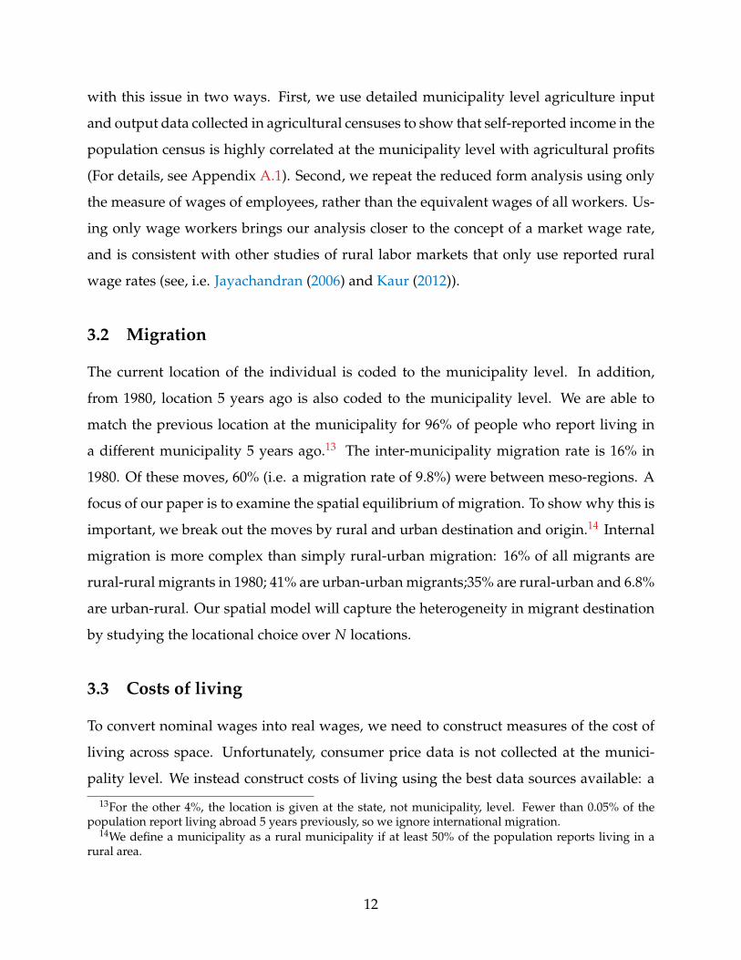
with this issue in two ways. First, we use detailed municipality level agriculture input

and output data collected in agricultural censuses to show that self-reported income in the

population census is highly correlated at the municipality level with agricultural profits

(For details, see Appendix A.1). Second, we repeat the reduced form analysis using only

the measure of wages of employees, rather than the equivalent wages of all workers. Us-

ing only wage workers brings our analysis closer to the concept of a market wage rate,

and is consistent with other studies of rural labor markets that only use reported rural

wage rates (see, i.e. Jayachandran (2006) and Kaur (2012)).

3.2 Migration

The current location of the individual is coded to the municipality level. In addition,

from 1980, location 5 years ago is also coded to the municipality level. We are able to

match the previous location at the municipality for 96% of people who report living in

a different municipality 5 years ago.13 The inter-municipality migration rate is 16% in

1980. Of these moves, 60% (i.e. a migration rate of 9.8%) were between meso-regions. A

focus of our paper is to examine the spatial equilibrium of migration. To show why this is

important, we break out the moves by rural and urban destination and origin.14 Internal

migration is more complex than simply rural-urban migration: 16% of all migrants are

rural-rural migrants in 1980; 41% are urban-urban migrants;35% are rural-urban and 6.8%

are urban-rural. Our spatial model will capture the heterogeneity in migrant destination

by studying the locational choice over N locations.

3.3 Costs of living

To convert nominal wages into real wages, we need to construct measures of the cost of

living across space. Unfortunately, consumer price data is not collected at the munici-

pality level. We instead construct costs of living using the best data sources available: a

13For the other 4%, the location is given at the state, not municipality, level. Fewer than 0.05% of thepopulation report living abroad 5 years previously, so we ignore international migration.

14We define a municipality as a rural municipality if at least 50% of the population reports living in arural area.

12

consumer price index collected at 10 cities in Brazil, and housing prices collected in the

population census. The national consumer price index is a data series collected by IBGE

for 10 locations across Brazil. For each AMC, we merge to the closest price collection

point. In the analysis, we will make an adjustment sourced from equations linking the

ability of a region to trade with other regions and source cheaper products to generate

a measure of the change in price indices. Second, we use rental rates from the popula-

tion census. Approximately 15% of our sample (and 30% of migrants), report paying rent

to live in their accommodation. We construct the mean rental rate per bedroom at the

municipality level. The mean rental rate for one bedroom is 129 Reals a month in 1980,

equivalent to 37 hours of work at the mean wage. We show in Appendix A.2 that rental

rates are positively correlated with the relative price index.15

3.4 Road data

Our geographic data come from two sources. We obtained vector-based maps from the

highway network for the period 1960 to 2000 from the Brazilian Ministry of Transporta-

tion. These maps were constructed based on statistical yearbooks from the Ministry’s

Planning Agency, previously known as GEIPOT. We used the ArcGIS software to georef-

erence the maps to match real-world geographic data. The geographic coordinate system

applied to the maps is the SIRGAS 2000.

The second source of data is the IBGE, which provides municipality boundaries maps

in digital format. We use the municipality boundaries from 2000 and apply the crosswalk

that maps the municipalities that existed in 2000 into AMCs.16. We also use the meso-

region codes defined by the IBGE to group municipalities into 131 meso-regions. Similar

to the road data, we applied the coordinate system SIRGAS 2000 to the AMC and meso-

region boundaries. Finally, in order to compute geographic distances in kilometers, we

projected the maps using the Brazil Mercator projection.

In our migration cost function, we use two variables to measure the cost of moving

15We also have producer level agricultural prices at the municipality level, sourced from the agriculturalcensus. This has not been incorporated in the analysis yet; for some preliminary analysis of how theseprices correlated with the consumer price index see Appendix A.2.

16The crosswalk file can be obtained from http://www.ipeadata.gov.br/

13

between two locations. The first variable is the Euclidean distance, which is computed

using the latitude and longitude coordinates of each origin-destination pair. The second

variable measures the distance between origin-destination pairs taking into account the

actual road coverage. To compute the latter, we use the fast marching algorithm, follow-

ing the approach used in Allen and Arkolakis (2014).17 First, we generate a picture of

the road network and the location of the 131 meso-regions. This picture is converted into

pixels and a travel speed is assigned to each pixel. Pixels corresponding to a paved road

are assigned a travel speed of 100, whereas pixels outside the road network are assigned

a travel speed of 0.00001. Essentially, this algorithm finds the shortest route, traveling on

roads, between two locations, with the minimum off-road traveled to connect a region

without a road to the road network. The outcome is a 131x131 matrix where each entry

corresponds to the fastest arrival time between a origin-destination pair. We undertake

the same exercise for our predicted highway system (the MST network) to find an instru-

ment for the actual bilateral cost using the travel time on the exogenous road network.18

For each year, the bilateral distances were normalized using the travel distance between

the nothernmost and the southernmost meso-regions as a nummeraire. The value used

when estimating the model is the predicted values from a regression of the actual bilateral

distances on the MST bilateral distances, including year fixed effects.

3.5 Trade data

For 1970, we source internal trade data for Brazil from the Anuario estatstico do Brasil

(IBGE, 1972), which is based on data from the Comercio Interestadual por vias Internas. The

survey provides information on the quantity (in tons) and the commercial value of ex-

ports and imports by type of goods and destination states. For the year 1999, we use data

from de Vasconcelos and de Oliveira (2006), consisting of interstate bilateral flow data are

17The fast marching algorithm finds the solution to the Eikonal equation used to characterize the prop-agation of wave fronts. The algorithm uses a search pattern for grid points in computing the arrival times(distances) that is similar to the Dijkstra shortest path algorithm (Hassouna and Farag (2007)). However,because the fast marching algorithm is applied to a continuous graph, it reduces the grid bias and generatesmore accurate bilateral distances.

18See Section 2 for details on the MST network.

14

derived from information on state tax.19

3.6 Geographic Units

Municipality boundaries change over time. In order to analyze the same geographical

area, we use data aggregated to two geographical regions. The first are the minimum

comparable areas (areas minimas comparaveis) constructed by the Institute of Applied Eco-

nomic Research in Brazil. We refer to these units as AMCs, or municipalities for short

hand. There are 3659 AMCs in Brazil in the period 1970 to 2000. The second unit of anal-

ysis are meso-regions. Meso-regions are statistical regions constructed by the Brazilian

Institute of Geography and Statistics (IBGE). There 3659 were grouped into 131 meso-

regions.20 We present statistics where possible at the finer level of geography; however, it

is not possible to estimate a dynamic choice model over 3659 dimensions, and so for the

estimation of the spatial model we instead use the coarser geography.

4 Reduced Form Evidence

The distribution of wages at the municipality level is shown in Figure 1. Each observation

is one municipality-year. We plot the distribution of log wages. In addition, we show the

cut-offs for the 90th and 10th percentile of the distribution; a measured commonly used

when analyzing productivity gaps within and across countries (see, for example, Caselli

(2005)).

The first plot in Figure 1 shows the wage distribution adjusting only for year fixed

effects. The 90/10 wage gap is 3.2: on average, municipalities at the 90th percentile of

the wage distribution have wages 3 times wages at the 10th percentile. However, there

could be many explanations for this difference: people have different education levels

or working in different industries which have different wages. The overlaid distribution

19The state tax is the Imposto sobre Operacoes relativas a Circulacao de Mercadorias e Prestacao de Servicosde Transporte Interestadual e Intermunicipal e de Comunicacao, or ICMS. This is a tax changed when there ismovement of goods, transportation, and communication services between states.

20There are 137 meso-regions defined by IBGE. However, there is not a perfect match between 6 meso-regions and the consistent municipalities and so we drop these 6 from the analysis.

15

controls for a host of individual level characteristics (schooling, age and industry worked)

as well as our best measures of the cost of living. Adjusting for these characteristics, the

90/10 wage gap is 2.1. Municipalities at the 90th percentile of the distribution have real

wages more than twice those at the 10th percentile.

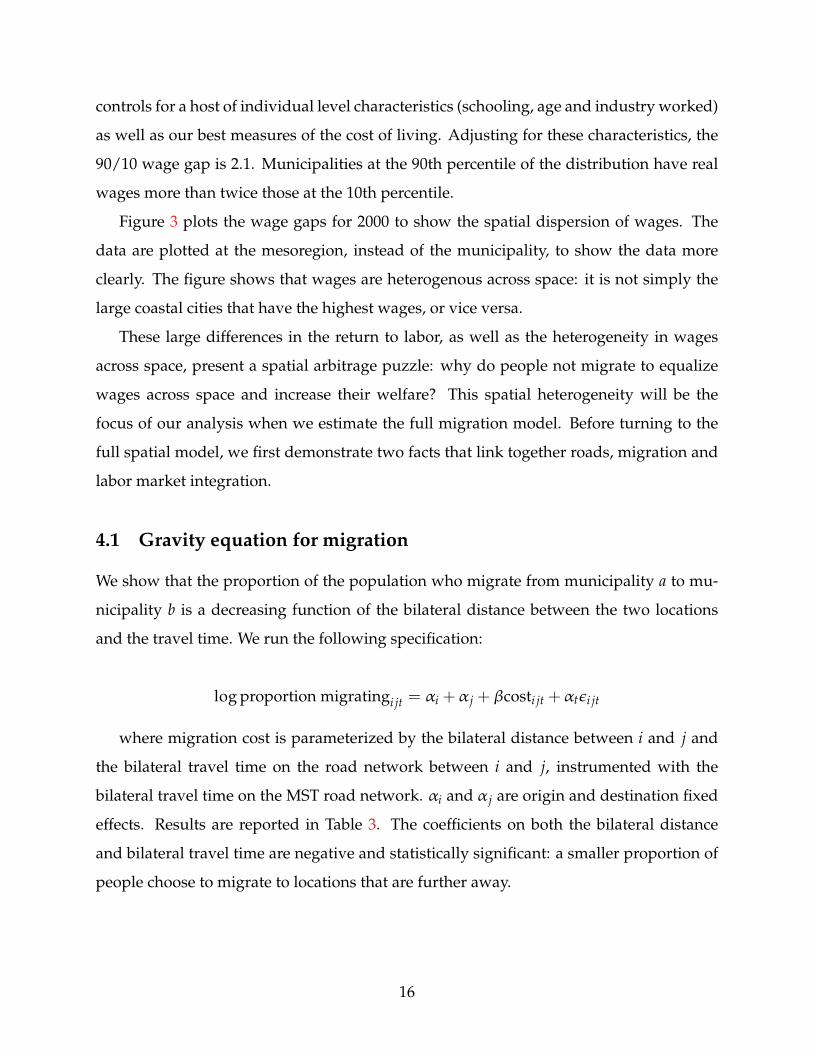
Figure 3 plots the wage gaps for 2000 to show the spatial dispersion of wages. The

data are plotted at the mesoregion, instead of the municipality, to show the data more

clearly. The figure shows that wages are heterogenous across space: it is not simply the

large coastal cities that have the highest wages, or vice versa.

These large differences in the return to labor, as well as the heterogeneity in wages

across space, present a spatial arbitrage puzzle: why do people not migrate to equalize

wages across space and increase their welfare? This spatial heterogeneity will be the

focus of our analysis when we estimate the full migration model. Before turning to the

full spatial model, we first demonstrate two facts that link together roads, migration and

labor market integration.

4.1 Gravity equation for migration

We show that the proportion of the population who migrate from municipality a to mu-

nicipality b is a decreasing function of the bilateral distance between the two locations

and the travel time. We run the following specification:

log proportion migratingi jt = αi +α j +βcosti jt +αtεi jt

where migration cost is parameterized by the bilateral distance between i and j and

the bilateral travel time on the road network between i and j, instrumented with the

bilateral travel time on the MST road network. αi and α j are origin and destination fixed

effects. Results are reported in Table 3. The coefficients on both the bilateral distance

and bilateral travel time are negative and statistically significant: a smaller proportion of

people choose to migrate to locations that are further away.

16

4.2 Roads reduce pass-through of productivity shocks

Next, we turn to a measure of labor market integration. We show that roads reduce the

pass-through of exogenous productivity shocks. To do this, we estimate the specification

from Jayachandran (2006):

log wit = α1 log TFPit +α2roadsit +α3 log TFPXroadsit +εit

We construct productivity shocks in two ways. First, following Jayachandran (2006),

we construct a value-weighted yield measure using output of the four main crops pro-

duced in Brazil. We instrument crop yields with monthly rainfall. The second produc-

tivity shock we use is a local labor demand shock, known as a Bartik shift-share shock

Bartik (1991).21 Results are reported in Table 4. A positive productivity shock increases

wages; and the interaction between the productivity shock and access to roads is nega-

tive. This holds for both agricultural and non-agricultural wages, using either rainfall or

Bartik share-shifter shocks to instrument for productivity shocks. This is consistent with

roads affecting labor supply elasticity, for example through making migration less costly,

and hence increasing labor market integration between municipalities.

These results suggest a relationship between roads, wages, and migration. However,

to separately identify the effects of amenities, income and migration costs it is necessary

to estimate the fully specified spatial equilibrium model. This is what we turn to next.

5 Model

This section presents the spatial equilibrium model. The framework is based on Moretti

(2011). We augment the model by adding in pairwise location-specific migration costs as

well as costly trade of goods across space, following Eaton and Kortum (2002).

In the model, agents gain indirect utility from real wages and amenities, which vary

by location. Migration is costly and depends on the origin and destination. Agents choose

the location which maximizes their utility, and will migrate from the current location if

21The Bartik shock is described in Section 5.

17

the value of moving to another location and paying the cost to do so is higher than the

utility from remaining where they are. Nominal wage differences across locations reflect

productivity differences; real wages reflect differences in nominal wages and differences

in prices. Prices are determined by market access. The utility agents receive also depends

on the cost of living. Each location has a rental market, with a housing supply elasticity

that determines the response of rental rates to increased demand for housing. A location

that receives a positive productivity shock will have higher nominal wages. These nom-

inal wages will attract migrants. An inflow of migrants will increase the rental rate of

housing, hence reducing the real wage and reducing the returns to migration.

Differences in real wages across space can arise from both migration costs as well as

differences in amenity values. In the original Roback model of migration (Roback, 1982),

all agents are indifferent across locations, and differences in real wages are equal to the

difference in amenity value of locations across space. With an idiosyncratic taste com-

ponent for location, such as in Moretti (2011), the marginal, rather than the average, mi-

grant is indifferent across location. Introducing migration costs into the model generates

a wedge in utility for the marginal migrant. This can lead to larger gaps in real wages

than if labor were perfectly mobile: without migration costs the agent may migrate, driv-

ing up rental rates in the destination and reducing them in the origin, hence reducing the

real wage gap between origin and destination. With migration costs, the agent no longer

migrates and so the wage differential is larger. The magnitude of these effects is the aim

of our empirical estimation.

We now set up the key ingredients of the model: equations specifying labor demand,

labor supply and housing supply, and show how these equations form the spatial equi-

librium system.

5.1 Labor demand

The production side of the economy is based on a standard model of locations producing

goods based on their comparative advantage (Eaton and Kortum, 2002; Redding, 2014).

Assume that there is a continuum of goods, m ∈ [0, 1], which are produced in each loca-

18

tion j at time t according to the following production function:

Yjt(m) = z jt(m)Lαjt(m)

where z jt(m) is location- and good-specific productivity and L jt(m) is labor.

Because labor markets are competitive, labor is paid its marginal revenue, so that

w jt(m) = p jt(m)αz jt(m)Lα−1jt (m)

where w jt(m) is the nominal wage paid to workers in location j in time t and p jt(m)

is the unit price a firm receives from selling the good. We assume that α is equal to

one, which is equivalent to assuming perfect capital mobility (i.e. Moretti (2011)).22 Each

location must have the same wage across goods it it producing. From this assumption,

we derive the labor demand function for location j in time t as

w jt = p jt(m)z jt(m)∀m (1)

which implies that labor demand is only a function of location and good-specific produc-

tivity. Additionally, nominal wage differences between two locations reflect productivity

differences and differences in producer prices.

5.2 Price determination

We allow for trade between two locations to take place and affect the local prices faced by

consumers (Eaton and Kortum (2002), Redding and Turner (2014)). The cost in location j

in time t of a good of type m made in location k is:

p jkt(m) = d jkt pkt(m)

where d jkt ≥ 1 are shipping costs. The shipping cost is the amount of the good that

22The implication that capital is perfectly mobile and therefore nominal wage differences purely reflectproductivity differences is a strong assumption. For a study that relaxes the perfect capital mobility as-sumption, see Ottaviano and Peri (2012).

19

needs to be shipped so that one unit of output from j arrives at k. We assume that good

markets are competitive, which implies that pkt(m) = MCkt(m) = wktzkt(m)

and

p jkt(m) = d jktwkt

zkt(m)

.

Location k’s productivity draw for each good m comes from a Frechet distribution

Fkt = e−Tktz−θ , where Tkt is the average productivity for location k in time t, and θ repre-

sents the productivity dispersion across goods.23 Consumers in location j purchase each

good from the locations that produce the good at the lowest cost. Therefore, using the

properties of the Frechet distribution yields an expression for the share of trade flows

into j from k:

X jkt

Yjt=

Tkt(d jktwkt

)−θ∑s∈N Tst

(d jstwst

)−θ (2)

Additionally, from the CES preferences for goods we can derive a consumer price

index for location j as follows:

Pjt = γ

[∑

s∈NTst(d jstwst

)−θ]−1θ

(3)

5.3 Housing markets

All housing is owned by absentee landlords. The elasticity of rental rates to labor is given

by:

log r jt = log ht + ηhouse log L jt (4)

where ηhouse is the elasticity of house prices to population. If it is easy to expand the

housing supply (for example, there is a lot of available land), then ηhouse will be small. If

it is not easy to expand the housing supply (for example, very strict zoning regulations),

then ηhouse will be large: the price of housing will increase a lot when there is a larger

23Productivity shocks are independent across goods, locations, and time.

20

workforce. Each worker demands one unit of housing, so the equilibrium in the housing

market will equate housing supply with labor supply.

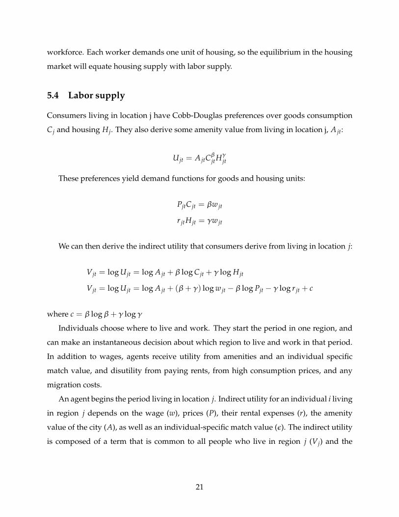
5.4 Labor supply

Consumers living in location j have Cobb-Douglas preferences over goods consumption

C j and housing H j. They also derive some amenity value from living in location j, A jt:

U jt = A jtCβjtH

γjt

These preferences yield demand functions for goods and housing units:

PjtC jt = βw jt

r jtH jt = γw jt

We can then derive the indirect utility that consumers derive from living in location j:

Vjt = log U jt = log A jt +β log C jt +γ log H jt

Vjt = log U jt = log A jt + (β+γ) log w jt −β log Pjt −γ log r jt + c

where c = β logβ+γ logγ

Individuals choose where to live and work. They start the period in one region, and

can make an instantaneous decision about which region to live and work in that period.

In addition to wages, agents receive utility from amenities and an individual specific

match value, and disutility from paying rents, from high consumption prices, and any

migration costs.

An agent begins the period living in location j. Indirect utility for an individual i living

in region j depends on the wage (w), prices (P), their rental expenses (r), the amenity

value of the city (A), as well as an individual-specific match value (ε). The indirect utility

is composed of a term that is common to all people who live in region j (Vj) and the

21

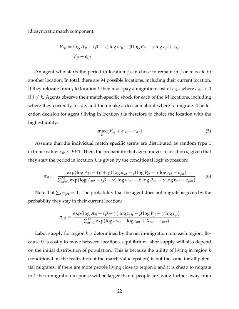
idiosyncratic match component:

Vi jt = log A jt + (β+γ) log w jt −β log Pjt −γ log r jt +εi jt

= Vjt +εi jt

An agent who starts the period in location j can chose to remain in j or relocate to

another location. In total, there are M possible locations, including their current location.

If they relocate from j to location k they must pay a migration cost of c jkt, where c jkt > 0

if j 6= k. Agents observe their match-specific shock for each of the M locations, including

where they currently reside, and then make a decision about where to migrate. The lo-

cation decision for agent i living in location j is therefore to choice the location with the

highest utility:

maxk{Vkt +εikt − c jkt} (5)

Assume that the individual match specific terms are distributed as random type 1

extreme value: εik ∼ EV1. Then, the probability that agent moves to location k, given that

they start the period in location j, is given by the conditional logit expression:

π jkt =exp(log Akt + (β+γ) log wkt −β log Pkt −γ log rkt − c jkt)

∑Mm=1 exp(log Amt + (β+γ) log wmt −β log Pmt −γ log rmt − c jmt)

(6)

Note that ∑k π jkt = 1. The probability that the agent does not migrate is given by the

probability they stay in their current location:

π j jt =exp(log A jt + (β+γ) log w jt −β log Pjt −γ log r jt)

∑Mm=1 exp(log wmt − log rmt + Xmt − c jmt)

Labor supply for region k is determined by the net in-migration into each region. Be-

cause it is costly to move between locations, equilibrium labor supply will also depend

on the initial distribution of population. This is because the utility of living in region k

(conditional on the realization of the match value epsilon) is not the same for all poten-

tial migrants: if there are more people living close to region k and it is cheap to migrate

to k the in-migration response will be larger than if people are living further away from

22

region k and it is expensive to migrate there. In a world without bilateral migration costs,

labor supply does not depend on the distribution of population because the cost does not

differ based on current origin - people migrate to region k if it provides the highest level

of utility, independent of their current location.

Given the initial distribution of the population, N j,t−1, ∀ j = 1, 2, ..., M, the labor sup-

ply in locality k is the net inflow of labor into region k from every region (including those

who start in k and chose not to migrate out):

Lkt =M

∑j=1

π jktN j,t−1

=M

∑j=1

exp(log Akt + (β+γ) log wkt −β log Pkt −γ log rkt − c jkt)

∑Mm=1 exp(log Amt + (β+γ) log wmt −β log Pmt −γ log rmt − c jmt)

N j,t−1 (7)

5.5 Spatial equilibrium

The spatial equilibrium is given by solving a system of simultaneous equations for gross

migration from j to k (π∗jkt), equilibrium labor (L∗kt), wage (w∗kt), price (P∗kt), and housing

quantities (r∗kt) for each region k, such that:

1. Labor demand is given by equation 1:

w∗jt = P∗jtz jt

2. Price index is given by equation 3:

P∗jt = γ

[∑

s∈NTst(d jstw∗st

)−θ]−1θ

3. Housing supply is given by equation 4:

log r∗kt = log ht + ηhouse log L∗kt

23

4. Migration rates are given by 6:

π∗jkt =exp(log A jt + (β+γ) log w∗jt −β log P∗jt −γ log r∗jt − c jkt)

∑Mm=1 exp(log Amt + (β+γ) log w∗mt −β log P∗mt −γ log r∗mt − c jmt)

5. Labor supply is given by equation 7:

L∗kt =M

∑j=1

π∗jktN j,t−1

The spatial equilibrium yields that the marginal migrant is indifferent between staying

in their current location and migrating. In a world where migration was costless, the

marginal migrant would receive the same utility at each location. However, with costly

migration, the marginal migrant internalizes the cost of migrating and will only migrate if

the utility at the new destination is large enough to compensate for the cost of migrating.

Migration costs therefore introduce a wedge in utility across locations.

6 Estimation

This section describes the procedure to estimate the spatial equilibrium model. Consider

an initial spatial equilibrium where the number of people in region j at time t is given by

N jt. The economy experiences productivity shocks in period t + 1, which generate new

wage shocks for each location. The productivity shocks propagate through the economy.

Initially, the productivity shock in k increases nominal wages in region k, and will also

decrease the price of that good produced in k. This will increase the returns to migrating,

and so people from every other region will migrate into k. At the same time, trade will

increase with other locations, as the price of the good produced in k has now decreased.

As labor migrates in, the demand for housing increases, pushing up the rental rate for

housing. As trade increases, the overall effect on the price index is smaller, decreasing

real wages. The rate of increase of rental rates will depend on the elasticity of housing

to population. As the rental rate for housing increases, the real return to migration to

region k decreases. Agents will continue to migrate into k until the marginal migrant is

24

indifferent between staying in their initial region j and migrating to k. The new spatial

equilibrium is the allocation of individuals across space, N j,t+1. The goal of the estimation

is to predict the new spatial allocation as closely as possible.

To estimate the model we implement a two-step estimator, following Diamond (2013),

based on a two-step BLP estimator. We need to estimate one more adjustment process -

the effect of market access on prices - in order to convert nominal wages into real wages.

The first step of the estimation process is to estimate the common utility for each region

separately from the transportation cost. We then estimate a trade-cost model to construct

a weighted index of market access. We then use the change in the common utility over

the 10-year census periods to identify the parameters determining the spatial equilibrium

process: elasticities of utility to changes in rents and wages, and elasticity of house prices

to changes in population, and the effect of the change of wages on the change in consumer

prices, using the relationship derived from the market access index. We use three sets of

instruments to identify the model. To identify the effect of roads on migration costs in the

first stage estimation, we use the instrument generated by the construction of highways

linking Brasilia with state capitals. To identify the spatial adjustment parameters in the

second stage we use a combination of moment conditions derived from initial conditions

(the population distribution across space) and exogenous productivity shocks.

6.1 First stage: estimation of transportation costs

The first stage of the estimation process is to use the observed gross migration flows to

separately estimate the common utility (Vj) from the transport cost (c jk). A key part of our

analysis is to identify the bilateral migration costs of moving between j and k. In order

to estimate these costs, it is necessary to have data on gross migration flows, not just the

net population allocation.This is because due to preference shocks, in the data we will see

observationally equivalent people migrating between j and k in both periods in response

to the same wage shock. Our analysis is similar to the approach used for identifying costs

of switching industries in Artuc et al. (2010).

From equation 6, the gross migration flows between j and k are given by the following

25

equation, which takes the form of a conditional logit:

π jkt =exp(log wkt

Pkt− log rkt + Xkt − c jkt)

∑Mm=1 exp(log wmt − log rmt + Xmt − c jmt)

=exp(Vkt − c jkt)

∑Mm=1 exp(Vmt − c jmt)

We assume a parametric form for c jkt, consisting of a common component across all

migrants, and a variable component depending on the pairwise migration move:

c jkt = αt +βX jkt (8)

The vector X jkt will include variables such as the Euclidean distance between j and k

as well as a measure of the road coverage between the two locations. The specification

for transportation costs is discussed further in the empirical section.

The likelihood function is constructed from the observed location choices. Consider

individual i j who was living in location j at the end of period t− 1. In total, N j people

were in location j at the end of period t− 1. In period t, each individual i j has moved to

location k with probability Pjkt. The likelihood function is therefore:

LLL((Vk,t)Mk=1,α,β) = ∑

j∑k

N j

∑i j

I(di j = k)Pjkt

LLL((Vk,t)Mk=1,α,β) = ∑

j∑k

N j

∑i j

I(di j = k)exp(Vk,t − I(k 6= j)(αt +βX jkt))

∑Mm=1 exp(Vm,t − I(m 6= j)(αt +βX jmt))

(9)

The likelihood function is globally concave and can be estimated by maximum like-

lihood. The first stage of the estimation therefore uses observed migration flows and

extracts the migration cost coefficients and the location-specific utilities.

26

6.2 Second stage: estimate of trade costs

The second stage we estimate the parameters determining costly trade across space. From

equation 2, trade flows are given by:

X jkt

Yjt=

Tkt(d jktwkt

)−θ∑s∈N Tst

(d jstwst

)−θTherefore, we estimate a fixed effects gravity equation:

log X jk = α j + log roads jk + log distance jk︸ ︷︷ ︸log d jk

+αk +ε jk

This yields the coefficients for d jst, ∀ j, s. Then, we log-linearize the price index 3 to

yield:

log Pnt = ∑i∈N

(Ti

d−θnit

∑s∈N d−θn jt

)log w

−1θ

it

This gives an adjustment to capture “market access” term in our third stage (we in-

strument wage shocks so only consider own shock wi):

∆ log Pit = −1θ

1

∑s∈N d−θn jt∆ log wit

6.3 Third stage: estimation of spatial equilibrium

Once we have recovered the mean level of utility for each region Vjt, we then relate this to

observable changes in wages and rents that occurred over this period. We estimate four

structural parameters: the elasticity of utility to real wages, γw, the elasticity of utility

to rents, γr, the elasticity of wages to productivity shocks, αA, and the elasticity of rental

rates to population ηhouse. To estimate these parameters, we use a GMM estimation proce-

dure. We construct exogenous productivity shocks to use as instruments for productivity

differences across space. In addition, we use initial conditions to generate moments to

generate an over-identification test of the model.

27

The specific productivity shock we construct will be a Bartik shock (Bartik (1991)).24

The Bartik shock takes the national-level growth rate in wages for each industry, and

constructs a region specific wage shock based on the initial industry specialization of

each region. Precisely, we compute the nation-wide increase in wages for each industry

between period t and period t + 1 and then assign a predicted wage shock to region k,

based on the baseline composition of industry in region k. Let the Bartik shock for region

k be given by ∆Bk,t+1 = Bk,t+1 − Bkt :

∆Bk,t+1 = ∑ind

(∆ log wind,−k,t+1)Lind,k,t

Lk,t

where log wind,−k,t is the average log wages in industry ind in year t, excluding work-

ers in region k. The Bartik shocks utilizes variation across space in the location of industry.

The second set of instruments we will use to construct moment inequalities in the

estimation procedure is the initial allocation of people across space, N jt.

The change in indirect utility for region k between period t + 1 and t is given by:

∆Vk,t+1 = αw∆ logwk,t+1

pk,t+1−αr∆ log rk,t+1 + ∆Xk,t+1

That is, utility is composed of differences in real returns across space. We assume that

location amenities change exogenously, so ∆X j,t+1 = αt.

∆Vk,t+1 = αw∆ logwk,t+1

pk,t+1−αr∆ log rk,t+1 +αt

We have recovered ∆Vk,t+1 from the first stage estimation equation. We now use the

equations that explain the spatial equilibrium model to estimate the underlying parame-

ters of the spatial equilibrium model.

6.3.1 Labor demand

The Bartik instrument provides variation in the productivity shock for region k:

24Bartik shocks are extensively used in urban economics to generate spatial productivity differences. Forrecent examples, see for example Diamond (2013); Notowidigdo (2013). They have been less extensivelyused in developing countries, one exception is Theoharides (2013) who studies the effect of migrant demandshocks in the Philippines.

28

∆ log wk,t+1 = αA∆Bk,t+1 +εwk,t+1

The identifying assumption is that the error term in the labor demand equation is not

correlated with the Bartik shock. In addition, the initial allocation of population is pre-

determined, so we require that the error term is not correlated with the initial population

Nkt:

E(∆Bk,t+1εwk,t+1) = 0

E(Nk,tεwk,t+1) = 0

6.3.2 Housing supply

Housing supply depends on the elasticity of house prices to population increases. The

Bartik shock identifies the house price elasticity through the predicted in-migration of

labor in response to the realized productivity shock, and allowing a trend constant across

all regions (αt).

∆ log rk,t+1 = ηhouse∆ log Lk,t+1 +αt +εrk,t+1

Identifying restrictions:

E(∆Bk,t+1εrj,t+1) = 0

E(Nkεrj,t+1) = 0

Together, these set of instruments identify the structural parameters determining the

effect of wages on indirect utility, γw, the effect on rents on indirect utility, γr, the elasticity

of wages to productivity shocks,αA, and the elasticity of rental rates to population ηhouse.

In the estimation, we normalizeγr to be 1, and so we estimate the relative weight of wages

to utility in the utility function.

29

7 Structural results

We first present the estimates for the spatial equilibrium model. We next use the estimates

to construct counterfactuals.

7.1 Estimation of parameters

The estimation occurs in three stages. The first stage of the estimation procedure is to

estimate the indirect utility for each location and the migration cost function. The second

stage is to estimate the cost of shipping goods across space and construct a market access

index. The third stage is decompose the change in utility into the change in real wages,

rents and amenities.

7.1.1 Estimation of migration costs

We specify the migration cost function as

c jkt = αt +β1Euclidean distance jk +β2highway distance jkt, ∀ j 6= k

The intercept of the cost equation, αt, measures the fixed cost of migration. The other

two coefficients measure variable costs of migration, depending on origin and destina-

tion. For each bilateral pair, we include both the euclidean distance between the two

locations, as well as the travel distance based on the existing road networks. Because the

road network is likely endogenous, we instrument it by the travel time on the predicted

MST network.

The migration cost function is identified by looking at the gross flows of migrants.

Agents who can travel to a region more cheaply will respond more to a given wage shock

in that region.25 This variation in migration responses at origin, given the same wages in

destination, identifies the migration cost separately from the utility gained once the desti-

nation is reached. The actual migration cost occurred will also depend on the destination

25Part of this cost may also be that people who live closer to major highways have better informationabout the wage rates in other locations. We include this reduction in the costs of acquiring information aspart of the cost reduction of roads.

30

chosen: for example, destinations that are further away may incur a large migration cost

that destinations that are closer and easier to migrate to. We capture this by including

the Euclidean distance between the centroids of each region. The gross migration flows

follow a gravity model, and so if it is more costly to travel longer distances we would

expect to see a positive coefficient for β1 and β2. If people dislike migration, as has been

found in many other studies, then we would expectαt to also be positive.

Note that the identification assumptions for the first stage results are relatively min-

imal. Because we do not explicitly model wages and rental rates in this stage, instead,

capturing them in a destination fixed effect, identification comes from the fact that we

have bilateral migration moves for each destination. In particular, any concerns about the

determinants of wages do not affect the identification of the migration cost as long as all

individuals face the same rental, wage and amenity markets once they have reached the

destination.

We estimate the migration cost function by estimating a conditional logit, using the

likelihood function specified in Equation 9. The point estimates are reported in Table 5.

All components of the migration cost are positive, as expected, and strongly statistically

significant: migration costs are a significant component in the decision of whether, and

where, to migrate. The fixed cost of migration is substantial. This coefficient reflects any

dislike of moving. The bilateral distance is positive and significant: traveling a longer

distance is more costly. However, the actual distance on a road is also strongly negative

and significant. This means that even controlling for the difference between two locations,

the actual travel time will affect the migration decision. This is important because neither

a dislike of moving nor Euclidean distance are variables that are under the control of

policy makers. However, distance on a road is a policy-relevant variable. We explore the

responsiveness of migration rates to changes in road travel time below.

Figure 4 shows the fit of the model from the first stage. The figure plots predicted

migration rates against the realized migration rates, where each point in the plot is a

bilateral pair. If no-one from the origin migrated, this would correspond to a migration

rate of 1 in the diagram for one bilateral point, and a migration rate of 0 for the N− 1 other

bilateral pairs. The graph shows that there is clustering around 0 and 1: for every location,

31

the most common migration destination is to not migrate, and on average, migration

rates are small to other regions. This is clear: the overall migration rate is 8.7%, so more

than 90% of people are non-migrants. The fit of the data is good: the R-squared from

a regression of actual migration rate of predicted migration rate is above 0.995 for each

year.

7.1.2 Estimation of trade costs

We specify the trade cost function as

d jkt = β1Euclidean distance jk +β2highway distance jkt +β3rail distance jkt, ∀ j 6= k

The trade cost function is identified from looking at bilateral gross trade flows. The

results are in Table 6. In all specifications, Euclidean distance is negative and statistically

significant.

The then use the implied measure of d jkt to compute a measure of market access at the

meso region:

εPjt ,p jt =1θ

1

∑s∈N d−θn jt

This index gives the elasticity of the equilibrium price index in one location to changes

in the price of the good it produces. The distribution of this index is graphed in Figure 5.

The elasticity ranges from 0.32 to 0.5. Meso regions that are well connected have a lower

elasticity - because they can trade easily with other locations, they export more of the

good they produce when they have a positive productivity shocks, and they import more

goods when their own goods are more expensive. Therefore, the pass through of shocks

into the CPI is smaller. However, meso regions who are not well connected, such as in

the North of the country with very little road access, or in the South of the country where

they are near the border with Uruguay and Paraguay, have much lower market access,

and hence, a higher elasticity of the consumer price index to own-productivty shocks.

32

7.1.3 Decompose indirect utility

The third step of the estimation recovers the underlying structural parameters that de-

termine the migration response to income shocks; the housing price response to labor

migration; and the wage response to TFP shocks. To estimate the model, it is necessary to

make an assumption about the production function, as such, the identification depends

on the production function specified. We estimate the second stage using two step GMM.

The point estimates are reported in Table 7. We show results with and without the adjust-

ment for consumer prices using the market access index. The elasticity of wages to TFP

is close to 1, which is as expected given that the Bartik shock is derived from mean wage

rates. The housing elasticity is 0.45, reflecting inelastic housing supply. This will be the

key variable that determines the general equilibrium effects of migration. The elasticity

of indirect utility to wages is 5.47 and statistically significant. The elasticity of utility to

rental prices has been normalized to -1 and is not reported in the table.

7.2 Welfare and migration effects of reducing travel costs

We now turn to the effect of migration costs on migration and welfare equalization across

space. Our model allows us to estimate partial equilibrium effects, and importantly, to

also compute the general equilibrium effects of migration, taking into account endoge-

nous responses of the housing market as agents migrate more in response to reductions

in migration costs. We highlight the magnitudes by undertaking two counterfactual pol-

icy exercises. We first compute the effect of the change in road access in partial equilib-

rium (holding all other endogenous variables constant). Next, we compute the general

equilibrium effect, allowing the endogenous response of the housing market to the in-

flow of new migrants. Without considering the general equilibrium effects the migration

response will be overstated.

The results are reported in Table 8. The results suggest a substantial effect on labor

allocation due to costs of migrating across space. In the data, 9.5% of adults aged over 20

migrated internally in 1980. If the average travel distance on a road was reduced by 50%

internal migration rates would increase to 13%, an increase of 40%. However, as people

33

migrate, there is an endogenous response of the housing market to an inflow of new

migrants. Column (2) shows the implied migration rate, taking into account the general

equilibrium response. On the extensive margin of migration, the general equilibrium

adjustment has a negligible effect on migration rates. However, as we will see, it will

generate differences in the level and dispersion of utility.

The second counterfactual experiment examines the migration response to a reduction

in the fixed cost of migration. Reducing the fixed cost of migration would increase inter-

nal migration rates to 46%. Here the the general equilibrium effects are approximately

2% smaller than the partial equilibrium effects, reflecting the endogenous reduction in

indirect utility as housing prices rise. However, fixed costs of migration may not be a pol-

icy relevant variable: this could easily capture the fact that people prefer to remain with

friends and family, and so reflects efficient non-migration. This is in contrast to the large

increase in migration rates from changing the marginal cost of migration, which does

provide evidence that access to transportation network impedes the efficient allocation of

labor across space.

We show the welfare effects of the policy that reduces the marginal cost of migrating

in Figure 6. The figure plots the distribution of indirect utility at baseline (estimated

from the data), and then after the reduction in migration costs, for each year. The dotted

line shows the partial equilibrium effects; the shaded line reflects the general equilibrium

effect. This would yield an increase in mean welfare of 8.1% (7.7% in GE), and a reduction

in the dispersion (standard deviation) by 6.2% (6.5% in GE). The mean increase in welfare

is reduced by 4.3% once the general equilibrium effects of migration are computed.

8 Conclusion

Wages in developing countries differ greatly across sector and across space. In Brazil,

the average wage in a municipality at the 90th percentile of the wage distribution is 3.2

times larger than the average wage in a municipality in the 10th percentile of the wage

distribution. Adjusting for individual characteristics, industry, and the cost of living, the

90/10 municipality wage gap is 2.1. These large differences in the return to labor present

34

a spatial arbitrage puzzle: why do people not migrate to equalize wages across space and

increase their welfare?

We propose one explanation: it is costly to move. To study the effect and magnitude of

migration costs on labor mobility, we construct a spatial equilibrium model. Our model

extends the standard spatial equilibrium model (Roback (1982); Moretti (2011)) to include

bilateral costs of migration and costly trade across space (Eaton and Kortum, 2002). We

use the construction of a planned capital city, Brasilia, to generate plausibly exogenous

variation in the national road network, and then examine whether having access to the

road network affects labor movement. We construct a novel dataset of bilateral inter-

municipality migration flows, covering 96% of the universe of internal migrants in Brazil

over the period 1980-2000. We first show that roads affect migration decisions and local

wages: i) a lower proportion of the origin population migrate to locations that are further

away, and ii) regions with road access have a lower pass-through of productivity shocks

into wages. Using the migration flow database and detailed data on the road network,

we then estimate the structural model to separate out the income, amenity and migration

effects of roads. The key result is that access to roads is an important determinant of

migration. Controlling for the euclidean distance between two location, reducing the

road distance by 50% would increase migration rates by 40%, and increase welfare by

over 8%. The welfare benefits are reduced by 4% once the general equilibrium effects of

migration are computed.

Our paper shows an important role for infrastructure in developing countries: facil-

itating the movement of labor to where their returns are highest. Costly migration can

generate inefficiencies in the allocation of labor across space. For example, a worker may

prefer to relocate to an area with a higher real wage, but the cost of moving may be too

high to make this decision optimal, reducing welfare. At an aggregate level, if certain

production locations require certain skills, the inability of labor to move easily may in-

creases the mismatch between labor and location, reducing productivity. The aggregate

effects of this misallocation, particularly for developing countries where infrastructure is

poor, is an important topic and will be pursued in future research.

35

References

Allen, Treb and Costas Arkolakis, “Trade and the Topography of the Spatial Economy,”Quarterly Journal of Economics, 2014, p. Quarterly Journal of Economics.

Artuc, E, S Chaudhuri, and J McLaren, “Trade shocks and labor adjustment: A structuralempirical approach,” The American Economic Review, 2010.

Banerjee, Abhijit, Esther Duflo, and Nancy Qian, “On the Road: Access to TransportationInfrastructure and Economic Growth in China,” 2009, pp. 1–22.

Bartik, Timothy J, “Who Benefits from State and Local Economic Development Policies?,”Books from Upjohn Press, 1991.

Baum-Snow, Nathaniel and Ronni Pavan, “Understanding the city size wage gap,” 2012.

Bird, Julia and Stephane Straub, “The Brasilia Experiment: Road Access and the SpatialPattern of Long-Term Local Development in Brazil,” 2014.

Bryan, Gharad and Melanie Morten, “The costs of spatial misallocation : Evidence fromIndonesia,” 2014.

Caselli, Francesco, “Accounting for Cross-Country Income Differences BT - Handbook ofeconomic growth,” in “Handbook of economic growth,” Vol. 1, Elsevier, 2005, pp. 679–741.

Chein, Flavia and Juliano Assuncao, “How does Emigration affect Labor Markets? Evi-dence from Road Construction in Brazil.,” 2009, pp. 1–32.

de Vasconcelos, Jose Romeu and Marcio Augusto de Oliveira, “Analise da Matrix popAtividade Economica do Comercio Interestadual no Brasil - 1999,” IPEA DIscussion Pa-per, 2006.

Diamond, Rebecca, “The Determinants and Welfare Implications of US Workers’ Diverg-ing Location Choices by Skill: 1980-2000,” 2013.

Eaton, Jonathan and Samuel Kortum, “Technology, Geography, and Trade,” Econometrica,2002, 70 (5), 1741–1779.

Epstein, D G, Brasilia: Plan and Reality, University of California Press, 1973.

Faber, Benjamin, “Trade Integration, Market Size, and Inudstrialization: Evidence fromChina’s National Trunk Highway System,” Review of Economic Studies, 2014.

Ghani, Ejaz, Arti Grover Goswami, and William R Kerr, “Highway to Success: The Im-pact of the Golden Quadrilateral Project for the Location and Performance of IndianManufacturing,” 2012.

36

Hassouna, M S and A A Farag, “MultiStencils Fast Marching Methods: A Highly AccurateSolution to the Eikonal Equation on Cartesian Domains,” Pattern Analysis and MachineIntelligence, IEEE Transactions on, 2007, 29 (9), 1563–1574.

Hornung, Erik, “Railroads and micro-regional growth in Prussia,” 2012.

Hsieh, Chang-Tai and Peter J Klenow, “Misallocation and Manufacturing TFP in Chinaand India,” Quarterly Journal of Economics, 2009, pp. 1–60.

IBGE, Anuario estatistico do Brasil - 1972 1972.

James, Preston and Spreidiao Faissol, “The Problem of Brazil’s Capital City,” GeorgraphicalReview, 1956, 46, 301–317.

Jayachandran, S, “Selling labor low: Wage responses to productivity shocks in developingcountries,” Journal of Political Economy, 2006.

Kaur, Supreet, “Nominal Wage Rigidity in Village Labor Markets,” 2012.

Kennan, J and J Walker, “The Effect of Expected Income on Individual Migration Deci-sions,” Econometrica, 2011.

Lagakos, David, Moll Benjamin, Tommaso Porzio, and Nancy Qian, “Experience Matters:Human Capital and Development Accounting,” 2012.

Mangum, Kyle, “A Dynamic Model of Cities and Labor Markets,” 2012.

Michaels, G, “The effect of trade on the demand for skill: evidence from the InterstateHighway System,” The Review of Economics and Statistics, 2008.

Moretti, Enrico, “Local Labor Markets,” Handbook of Labor Economics, 2011.

Morten, Melanie, “Temporary Migration and Endogenous Risk Sharing in Village India,”2013.

and Jaqueline Oliveira, “The Long-Run effects of Roads: Evidence from Planned Cap-ital Cities,” 2014.

Notowidigdo, Matthew, “The incidence of local labor demand shocks,” 2013.

Ottaviano, Gianmarco I P and Giovanni Peri, “Rethinking the effects of immigration onwages,” Journal of the European Economic Association, 2012, 10 (1), 152–197.

Redding, S J, “Goods Trade, Factor Mobility and Welfare,” NBER Working Paper, 2014.

Redding, Stephen and Daniel Sturm, “The Costs of Remoteness: Evidence from GermanDivision and Reunification,” The American Economic Review, 2008, 98 (5).

Redding, Stephen J and Matthew A Turner, “Transportation Costs and the Spatial Orga-nization of Economic Activity,” 2014.

37

Roback, J, “Wages, Rents, and the Quality of Life,” The Journal of Political Economy, 1982.

Sjaastad, L, “The costs and returns of human migration,” The Journal of Political Economy,1962.

Theoharides, Caroline, “The Effect of International Migration on Origin-Country Educa-tional Attainment,” 2013.

38

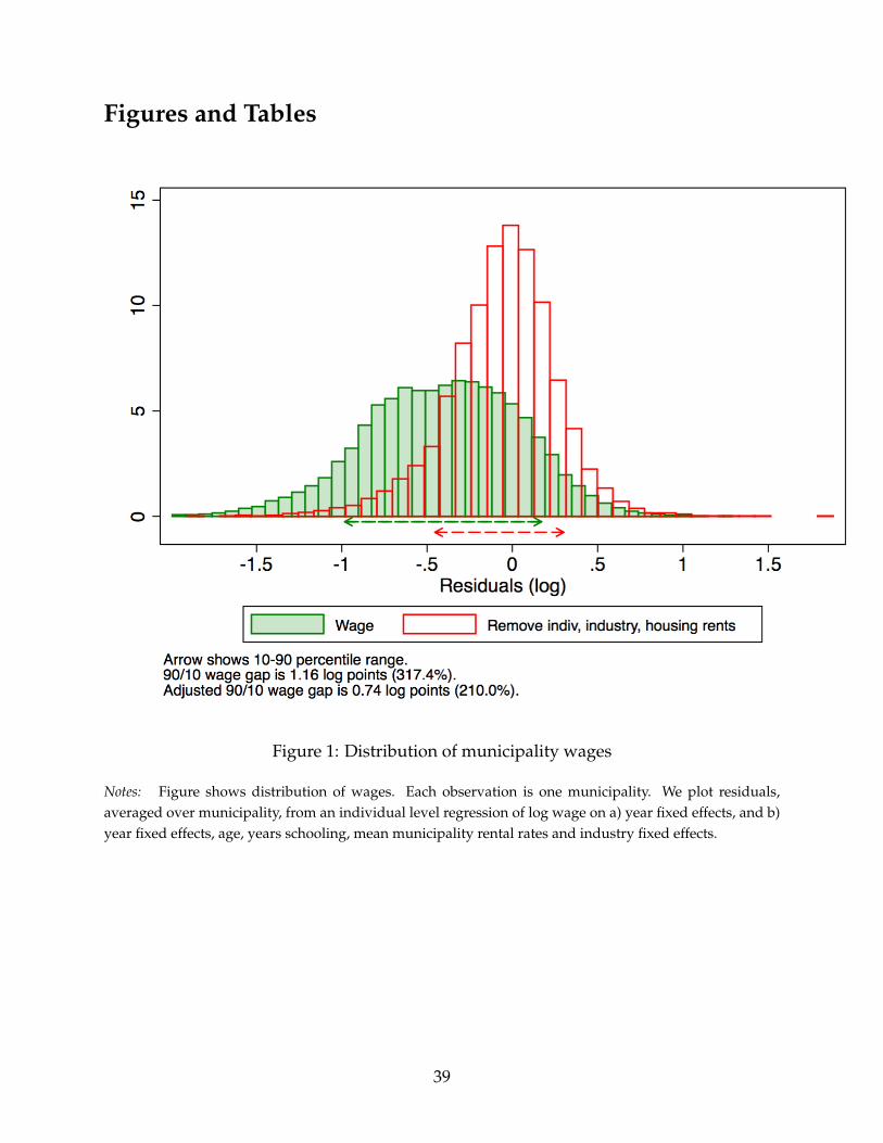
Figures and Tables

Figure 1: Distribution of municipality wages

Notes: Figure shows distribution of wages. Each observation is one municipality. We plot residuals,averaged over municipality, from an individual level regression of log wage on a) year fixed effects, and b)year fixed effects, age, years schooling, mean municipality rental rates and industry fixed effects.

39

Figure 2: Map of straight line instrument and radial highways

Notes: Figure shows Brasilia and the 26 state capitals. The map shows radial highways out of Brasiliaand the straight line instrument for roads. The straight line shows the minimum spanning tree instrumentbetween Brasilia and grouped state capitals. Source: Authors’ calculations based on maps obtained fromthe Brazilian Ministry of Transportation.

40

Figure 3: Wage gaps across space: removing individual and industry characteristics

Notes: Figure shows wage gaps, measured in log differences, across mesoregions in Brazil. Source: Au-thors’ calculations based on census data.

41

Figure 4: Predicted vs actual migration rates

Notes: Figure shows predicted migration rates again actual migration rates. Each dot is a bilateral mesoregion pair.Source: Authors’ calculations based on census data.

42

Figure 5: Index of market access

Notes: Calculated using spatial weight from price index. Places that are less connected (by road or bydistance) have a higher elasticity of their consumer price index to own shocks.

43

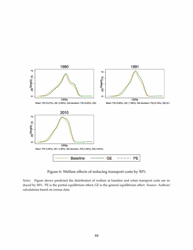
Figure 6: Welfare effects of reducing transport costs by 50%

Notes: Figure shows predicted the distribution of welfare at baseline and when transport costs are re-duced by 50%. PE is the partial equilibrium effect; GE is the general equilibrium effect. Source: Authors’calculations based on census data.

44

Table 1: First stage for straight line instrument

Log distance Indicator for road(1) (2) (3) (4)

Dep. variable: Dist. from paved road b/se b/se b/se b/se

Predicted road (log km) 0.113*** 0.148***(0.025) (0.041)

On straight-line path 0.111*** 0.163**(0.041) (0.064)

Area 0.000* 0.000***(0.000) (0.000)

Closer nearest big city -0.105** -0.038**(0.044) (0.018)

Closer to Brasilia 0.558* 0.206*(0.326) (0.121)

State FE Yes Yes Yes YesYear FE Yes Yes Yes Yes

R-Squared 0.497 0.515 0.563 0.570F-stat 20.5 12.7 7.3 6.4Number of municipalities 3659 3659 3659 3659

Notes: Table shows OLS regressions. Cols (1) and (2) show distance to nearest road asa function of the distance to the straight line distance between Brasilia and state capitals.Distances measured in log km. Col (3) regresses an indicator variable for having a pavedroad on an indicator variable for being on the straight line path. Stars indicate statisticalsignificance. ∗ ∗ ∗ < 0.01, ∗∗ < 0.05, ∗ < 0.1. Standard errors clustered at municipalitylevel..

45

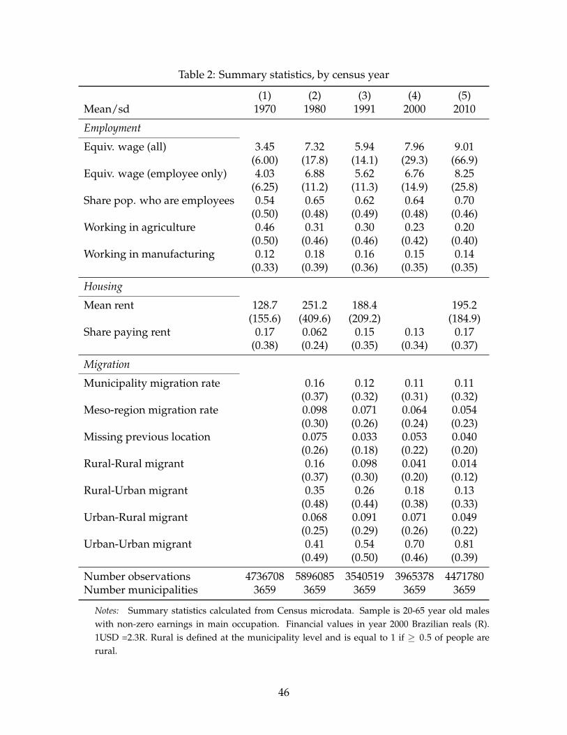
Table 2: Summary statistics, by census year

(1) (2) (3) (4) (5)Mean/sd 1970 1980 1991 2000 2010

Employment

Equiv. wage (all) 3.45 7.32 5.94 7.96 9.01(6.00) (17.8) (14.1) (29.3) (66.9)

Equiv. wage (employee only) 4.03 6.88 5.62 6.76 8.25(6.25) (11.2) (11.3) (14.9) (25.8)

Share pop. who are employees 0.54 0.65 0.62 0.64 0.70(0.50) (0.48) (0.49) (0.48) (0.46)

Working in agriculture 0.46 0.31 0.30 0.23 0.20(0.50) (0.46) (0.46) (0.42) (0.40)

Working in manufacturing 0.12 0.18 0.16 0.15 0.14(0.33) (0.39) (0.36) (0.35) (0.35)

Housing

Mean rent 128.7 251.2 188.4 195.2(155.6) (409.6) (209.2) (184.9)

Share paying rent 0.17 0.062 0.15 0.13 0.17(0.38) (0.24) (0.35) (0.34) (0.37)

Migration

Municipality migration rate 0.16 0.12 0.11 0.11(0.37) (0.32) (0.31) (0.32)

Meso-region migration rate 0.098 0.071 0.064 0.054(0.30) (0.26) (0.24) (0.23)

Missing previous location 0.075 0.033 0.053 0.040(0.26) (0.18) (0.22) (0.20)

Rural-Rural migrant 0.16 0.098 0.041 0.014(0.37) (0.30) (0.20) (0.12)

Rural-Urban migrant 0.35 0.26 0.18 0.13(0.48) (0.44) (0.38) (0.33)

Urban-Rural migrant 0.068 0.091 0.071 0.049(0.25) (0.29) (0.26) (0.22)

Urban-Urban migrant 0.41 0.54 0.70 0.81(0.49) (0.50) (0.46) (0.39)

Number observations 4736708 5896085 3540519 3965378 4471780Number municipalities 3659 3659 3659 3659 3659

Notes: Summary statistics calculated from Census microdata. Sample is 20-65 year old maleswith non-zero earnings in main occupation. Financial values in year 2000 Brazilian reals (R).1USD =2.3R. Rural is defined at the municipality level and is equal to 1 if ≥ 0.5 of people arerural.

46

Table 3: Gravity equation for migration

(1) (2)All pairs Only migrant pairs

Dep var: Prop. migrating b/se b/se

Log traveltime -8.29*** -36.5***(1.79) (8.47)

Log distance -0.88*** -0.58***(0.022) (0.059)

Origin FE Yes YesDestination FE Yes YesN 16061 15537

Notes: Data from 1980, 1991, 2000 and 2010 censuses. Each obser-vation is a bilateral meso-region pair (n=131). Total possible samplesize = 4 years*(1312) = 68, 644. Pairs dropped from regression ifzero pairwise migration. Robust standard errors reported.

Table 4: Roads reduce pass-through of productivty shocks.

Rainfall Shocks Bartik Shocks(1) (2) (3) (4)All Employees Baseline Adj. Labor

Dep var: Log wage b/se b/se b/se b/se

TFP shock 0.11*** 0.093** 0.91*** 1.00***(0.033) (0.031) (0.034) (0.035)

TFP X Road -0.21*** -0.21*** -0.24** -0.29**(0.054) (0.052) (0.090) (0.089)

Close to road 0.11 0.29** -0.34** -0.31**(0.12) (0.11) (0.12) (0.10)

N 10452 10452 16864 16864

Notes: Close to road is a dummy variable if the municipality is within the20th percentile distance to road, instrumented with the same definition for theinstrument. Robust standard errors clustered at municipality. Agriculturalshocks don’t include 2010 census as crop yields not available.

47

Table 5: Fixed and marginal costs of migration

(1) (2) (3) (4)1980 1991 2000 2010

Fixed cost of migrating 4.57*** 5.12*** 5.23*** 5.53***(0.0036) (0.0052) (0.0052) (0.0052)

Bilateral distance (km) 0.0020*** 0.0017*** 0.0017*** 0.0018***(0.0000040) (0.0000052) (0.0000050) (0.0000056)

Bilateral travel time 5.72*** 4.76*** 4.89*** 4.12***(0.025) (0.033) (0.032) (0.032)

No. individuals 5,370,772 3,219,779 3,575,695 3,991,674Mean migration rate 0.089 0.063 0.056 0.048Mean bilateral distance migrated 0.12 0.12 0.12 0.12Mean bilateral distance 0.16 0.17 0.17 0.16

Notes: Source: Brazilian Census data, 1980-2010. Table reports estimates from a conditional logit modelof migration. Location fixed effects estimated but not reported. Mean bilateral distance relative to N-SBrazil. Note: standard errrors should be boostrapped as distance to road is instrumented. This is inprogress.

Table 6: Trade gravity equations

1970 1999 Both(1) (2) (3) (4) (5) (6)

Dep. variable: Log trade b/se b/se b/se b/se b/se b/se

Log instrument distance -0.043** -0.047** -0.019 -0.018 -0.023 -0.018(0.019) (0.018) (0.017) (0.016) (0.019) (0.016)

Log distance -1.73*** -1.66*** -1.32*** -1.33*** -1.49*** -1.33***(0.11) (0.091) (0.085) (0.088) (0.067) (0.088)

Log rail distance -0.45 0.049 0.049(0.27) (0.24) (0.24)

Origin FE Yes Yes Yes Yes YesDestination FE Yes Yes Yes Yes YesYear FE Yes Yes Yes Yes YesNumber of obs 477 477 630 630 1107 630

Notes: Data is state-state bilateral trade flows.

48

Table 7: Structural coefficient estimates

No price correction With price correctionb/se b/se

Elasticity wages to TFP 1.01*** 1.01***(0.022) (0.022)

Elasticity rental rates to pop 0.45*** 0.45***(0.067) (0.065)

Elasticity utility to wages 5.47** 4.77**(2.64) (2.04)

Year FE Yes YesJ statistic 2.60 2.66p value 0.27 0.62

Notes: Estimated using 1980-2000 data. Coefficients calculated using two-step GMM.Elasticity of utility to rent normalized to -1. Robust standard errors provided. Overi-dentification J statistic and p-value provided.

Table 8: Counterfactual migration rates

1980 1991 2010(1) (2) (3) (4) (5) (6)PE GE PE GE PE GE

Migration rate

Baseline 0.095 0.095 0.060 0.060 0.048 0.048Reduce marginal cost by 50% 0.13 0.13 0.079 0.079 0.061 0.061Reduce fixed cost by 50% 0.46 0.45 0.43 0.43 0.43 0.43Data 0.094 0.094 0.062 0.062 0.050 0.050

Notes: Source: Brazilian Census data, 1980-2000. 1.5% sample. PE = partial equilibrium.GE = general equilibrium. Sample only individuals aged 20 and over. Table reportsestimates derived from structural estimation.

49

A Appendix

A.1 Self-reported agricultural income

In the Brazilian census, between 50-70% of the sample who report working in agriculture

are self-employed rather than employees.26 Self-reported income in censuses may not ac-

curately reflect agricultural wage income for at least three reasons: i) self-reported income

may be revenues, rather than income, ii) it may contain payments to both labor as well

as other factors of production such as capital, or iii) it may be more accurately provided

at the household, rather than the individual, level (Lagakos et al. (2012)). In this section

we use data from Brazilian agricultural censuses and present evidence that, despite the

potential problems, agriculture self-employment income as measured in population cen-

suses highly correlates with agriculture profits computed from agricultural censuses. In

addition, we run the reduced form analysis in the paper both including and excluding

non-employees, and results are robust.

Starting in 1970, the Agriculture Censuses were collected every five years. The agricul-

ture census allows us to measure agricultural income accurately as it covers the universe

of agricultural production unities, regardless of their size, output level, or location.27It is

worth mentioning that home gardens were not considered as agricultural unities for the

purpose of data collection. Nonetheless, we believe that we only miss some of the pro-

duction for own consumption of those who work mainly outside the agricultural sector.

We obtain the series of agriculture revenues and expenses at the AMC level from

IPEADATA. Agriculture revenue comprises proceeds from the sale of agricultural prod-

ucts, including final goods produced inside the agricultural unities, as well as revenues

from the rental of land and livestock and services rendered to third parts. Agriculture ex-

penses include expenses with wages, rents, other inputs, and operational expenses. Our

benchmark measure of AMC-level agricultural income is agricultural profits, as measured

by the difference between revenues and expenses. We used the years 1975, 1980, and 1996,

which are the closest to the population census years (1970, 1980 and 1991).

26The share of the population working in labor force declines from 46% in 1970 to 22% in 2010.27The agricultural censuses include unities located in urban areas.

50

Appendix Figure 1 displays the scatterplot of the agriculture (log) profits obtained

from the agriculture census against the agriculture self-employment (log) income com-

puted from the population census. The two income measures are positively correlated.

The R-squared from regressing the level of agriculture self-employment income on the

level of agriculture profits indicates is 0.80.

Appendix Figure 1: Comparison: population and agricultural censuses

51

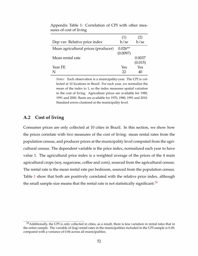
Appendix Table 1: Correlation of CPI with other mea-sures of cost of living

(1) (2)Dep var: Relative price index b/se b/se

Mean agricultural prices (producer) 0.026**(0.0097)

Mean rental rate 0.0037(0.015)

Year FE Yes YesN 22 40

Notes: Each observation is a municipality-year. The CPI is col-lected at 10 locations in Brazil. For each year, we normalize themean of the index to 1, so the index measures spatial variationin the cost of living. Agriculture prices are available for 1980,1991 and 2000. Rents are available for 1970, 1980, 1991 and 2010.Standard errors clustered at the municipality level.

A.2 Cost of living

Consumer prices are only collected at 10 cities in Brazil. In this section, we show how

the prices correlate with two measures of the cost of living: mean rental rates from the

population census, and producer prices at the municipality level computed from the agri-

cultural census. The dependent variable is the price index, normalized each year to have

value 1. The agricultural price index is a weighted average of the prices of the 4 main

agricultural crops (soy, sugarcane, coffee and corn), sourced from the agricultural census.

The rental rate is the mean rental rate per bedroom, sourced from the population census.

Table 1 show that both are positively correlated with the relative price index, although

the small sample size means that the rental rate is not statistically significant.28

28Additionally, the CPI is only collected in cities, as a result, there is less variation in rental rates that inthe entire sample. The variable of (log) rental rates in the municipalities included in the CPI sample is 0.49,compared with a variance of 0.84 across all municipalities.

52