Migration and Urbanisation in Post-Apartheid South …ftp.iza.org/dp10113.pdf · Migration and...

Forschungsinstitut zur Zukunft der ArbeitInstitute for the Study of Labor

DI

SC

US

SI

ON

P

AP

ER

S

ER

IE

S

Migration and Urbanisation inPost-Apartheid South Africa

IZA DP No. 10113

July 2016

Jan David BakkerChristopher ParsonsFerdinand Rauch

Migration and Urbanisation in Post-Apartheid South Africa

Jan David Bakker University of Oxford

Christopher Parsons

University of Western Australia and IZA

Ferdinand Rauch

University of Oxford and CEP

Discussion Paper No. 10113 July 2016

IZA

P.O. Box 7240 53072 Bonn

Germany

Phone: +49-228-3894-0 Fax: +49-228-3894-180

E-mail: [email protected]

Any opinions expressed here are those of the author(s) and not those of IZA. Research published in this series may include views on policy, but the institute itself takes no institutional policy positions. The IZA research network is committed to the IZA Guiding Principles of Research Integrity. The Institute for the Study of Labor (IZA) in Bonn is a local and virtual international research center and a place of communication between science, politics and business. IZA is an independent nonprofit organization supported by Deutsche Post Foundation. The center is associated with the University of Bonn and offers a stimulating research environment through its international network, workshops and conferences, data service, project support, research visits and doctoral program. IZA engages in (i) original and internationally competitive research in all fields of labor economics, (ii) development of policy concepts, and (iii) dissemination of research results and concepts to the interested public. IZA Discussion Papers often represent preliminary work and are circulated to encourage discussion. Citation of such a paper should account for its provisional character. A revised version may be available directly from the author.

IZA Discussion Paper No. 10113 July 2016

ABSTRACT

Migration and Urbanisation in Post-Apartheid South Africa* Under apartheid, black South Africans were severely restricted in their choice of location and many were forced to live in homelands. Following the abolition of apartheid they were free to migrate. Given gravity, a town nearer to the homelands can be expected to receive a larger inflow of people than a more distant town following the removal of mobility restrictions. Exploting this exogenous variation, we study the effect of migration on urbanisation and the distribution of population. In particular, we test if migration inflows led to displacement, path dependence, or agglomeration in destination areas. We find evidence for path dependence in the aggregate, but substantial heterogeneity across town densities. An exogenous population shock leads to an increase of the urban relative to the rural population, which suggests that exogenous migration shocks can foster urbanisation in the medium run. JEL Classification: R12, R23, N97, O18 Keywords: economic geography, migration, urbanisation, natural experiment Corresponding author: Christopher Parsons Economics (UWA Business School) University of Western Australia 35 Stirling Highway Crawley WA 6009 Australia E-mail: [email protected]

* We thank Daniel de Kadt and Melissa Sands who shared census data from 1991. We are grateful to Matteo Escudé, James Fenske, Doug Gollin, Vernon Henderson, Leander Heldring, Daniel Kaliski, Daniel de Kadt, Lu Liu, Chris Roth, Ludvig Sinander, Andrea Szabo, Tony Venables, Helene Verhoef, Johannes Wohlfart and seminar participants at Oxford and ABCA 2016 for useful comments and discussion. We gratefully acknowledge the support of an Africa Research Program on Spatial Development of Cities at LSE and Oxford funded by the Multi Donor Trust Fund on Sustainable Urbanization of the World Bank and supported by the UK Department for International Development.

1 Introduction

Consider the following thought experiment. What happens if a policy maker exogenouslyincreases the population of a random town? There are three possibilities, the town:may remain at the increased size, may revert back to its original level or it may finditself on a new growth trajectory and grow even further. Which of the three reactionsis observed may vary with the original size of the town as well as the magnitude of theshock. In answering this question we provide insights into the nature and evolution ofurbanised areas, the size and location of cities and the distribution of population in space.

In this paper, we use the abolition of mobility restrictions as a natural experiment, tostudy the effect of domestic migration on the distribution of population in post-apartheidSouth Africa. Under the apartheid regime, the black South African population wasseverely restricted in its mobility. Large parts of the population were forced to livein so-called homelands and townships. En-route to the democratic transition in 1994,these restrictions were lifted and in June 1991 black South Africans could move freelyfor the first time since the foundation of the state of South Africa in 1910. Substantialinternal migration flows resulted, which led to increased urbanisation during the 1990sand 2000s (see Figure 1 below).

The location of the homelands resulted from a long historical process beginning inthe 18th century (Lapping, 1986). It is therefore plausible to assume that their loca-tion, conditional on covariates, is quasi-random with respect to economic conditionstoday. Assuming the subsequent migration outflows from the homelands behavedaccording to gravity, we are able to exploit the exogenous effect of this positive mi-gration shock to identify the subsequent effects of increased internal mobility on thedistribution of population in South Africa. In other words, assuming migration costsincrease with distance, ceteris paribus, a town physically located nearer to a homeland isassumed to have received a larger inflow of previously mobility-restricted black migrants.

A town experiencing an exogenous migration shock can theoretically evolve in justthree ways. First, the town’s population could shrink back to the initial populationlevel, i.e. mean-revert. Such a reaction would be consistent with an optimal urbannetwork of relative city sizes, where relative sizes might be driven by location funda-mentals. Secondly, the town’s population could simply remain at the new populationlevel and not adjust endogenously to the shock. In this case, the distribution of citysizes would be path dependent. Thirdly, the city could grow further. This would beconsistent with a theory of multiple equilibria, where an initial population shock movesthe town onto a new population trajectory growth path from one equilibrium to another.

2

We provide quasi-experimental evidence that the aggregate population distribution ishighly path dependent. Distinguishing between rural and urban areas we find thatpopulation levels in areas with high initial population densities experience furtheragglomeration, i.e. there is endogenous in-migration after the shock. In rural areas,we cannot reject path dependent behaviour. This suggests that a positive exogenouspopulation shock generates a ‘Matthew effect’ (‘those who have will be given’), asdensely populated areas gain population relative to sparsely populated areas froman exogenous migration shock. We further investigate this heterogeneity by lookingat how the effect varies with both the initial population density and the reducedform size of the shock. We find that for a given initial density a bigger shock leadsto higher endogenous population growth. This is consistent with the idea that a sig-nificant shock is required to push a locality out of its current and into a new equilibrium.

Modifying the optimal city size model by Henderson (1974) we infer the shape of theagglomeration function from our empirical findings. In our version, agents’ utility isequal to the difference between the agglomeration function and the congestion cost curve.Assuming that the congestion cost curve is increasing and convex in population, we areable to relate our empirical results to the functional form of the agglomeration curve.The path-dependent evolution of the population level suggests that the agglomerationcurve has a slope similar to the congestion cost curve as a function of population density.This implies that an exogenous increase in population does not significantly affect theutility level of incumbents and suggests that there are infinitely many equilibria for thedistribution of population in space. The agglomeration effects in the densely populatedareas suggest that are potentially multiple equilibria in urban environments.

These results have important policy implications. Since positive population shocks havea permanent effect on the distribution of population in space, temporary policies thatinduce out-migration from some areas may influence the long-run distribution of citysizes. Such policies also affect the long-run distribution of population between rural andurban areas. Since the population increases more in urban than in rural areas, policiesthat induce migration also foster urbanisation. This suggests that policy makers areable to promote urbanisation and engineer the growth of metropolitan areas throughencouraging higher levels of migration. Conversely, policies that impede migration willhinder urbanisation.

The remainder of this paper is organised as follows. Section 2 discusses the relatedliterature, while section 3 details the historical development of South Africa thereby

3

providing evidence for the quasi-random location of the homelands. Section 4 introducesthe theoretical thought experiment that serves as a framework for the empirical analysispresented in Section 5. The heterogeneous responses to a positive population shock arediscussed in Section 6, while section 7 concludes.

2 Related literature

Our paper adds to the growing literature that exploits the exogenous variation resultingfrom apartheid policy to study the development of South Africa after 1994, see forexample de Kadt and Sands (2016), de Kadt and Larreguy (2016) and Dinkelman (2011,2013). We are the first to use this natural experiment to study the causal economiceffect of internal migration and how it effects the distribution of population in space.This paper, thereby, adds quasi-experimental evidence to the literatures that examinethe determinants of the uneven distribution of population in space and the relationshipbetween city size and population growth.

After Auerbach (1913) observed that the size distribution of cities follows a power law,there have been many attempts to explain this persistent empirical regularity (oftenreferred to as Zipf’s Law, after Zipf (1949)). Following the theoretical work by Gabaix(1999) who showed that Zipf’s Law emerges naturally if cities have equal relative growthrates (Gibrat’s Law), an extensive empirical literature on the distribution of populationhas developed. Davis and Weinstein (2002) find that the dispersion of populationis highly path-dependent and argue that this is due to the importance of locationfundamentals. They show that even after massive destruction and death caused bythe nuclear bombs, Hiroshima and Nagasaki rapidly returned to their pre-war growthpath. Studies by Brakman et al. (2004) for post-war Germany and by Miguel andRoland (2011) for Vietnam arrive at similar results. These studies though are unableto distinguish between the effects of path-dependence due to state-dependence (i.e.the presence of factors of production) and the importance of the initial natural advantage.

Bleakley and Lin (2012) therefore analyse path dependence by studying the devel-opment of towns that experienced a negative shock to their fundamentals, namelyportage cities that lost their natural trading advantage due to technological progress.This historical development allows the authors to disentangle state-dependence andthe natural advantage effect, since continuing agglomerations cannot be explained bynatural advantage. The main result of the study is that these former portage citiesmaintained their historical importance, a finding consistent with recent results from

4

local positive population shocks from German refugees after World War II that werehighly persistent and could not be explained by location fundamentals (Schumann, 2014).

We contribute to this literature in several ways. First, our study is the first to analysea large scale and indeed positive population shock. The studies of war destructionfind evidence of path-dependence but cannot isolate whether this is driven by naturalfundamentals, sunk investments, social networks or gains from agglomerations. Bleakleyand Lin (2012) provide evidence that it is not driven by location fundamentals, butcannot distinguish between other factors. Since we analyse a positive population shockin which incoming migrants have neither social networks nor private sunk investments,we are able to isolate the effect of gains from agglomeration. Secondly, we provideevidence from a credible natural experiment that is well-identified and are able todraw upon a much larger sample in estimation in comparison with most studies in thisliterature. Thirdly, we are the first to provide evidence from Africa, a region that isamongst the most rapidly urbanising regions in the world, the continent in which suchpolicies related questions matter most. Fourthly, many of the previous studies focussolely upon urban areas, whereas we are able to look at both rural and urban areas andthe differences between the two.

Our paper also speaks to the existing literature on the relationship between populationgrowth and the size of cities (e.g. Black and Henderson (2003), Eeckhout (2004),Duranton (2007), and Rossi-Hansberg and Wright (2007)). The majority of empiricalstudies find urban systems tend to obey Gibrat’s Law and that city size is uncorrelatedwith population growth, while others do find departures from Gibrat’s Law even forcities (Soo (2007), González-Val et al. (2013), and Holmes and Lee (2010)). Michaelset al. (2012) emphasise the importance of structural transformation for urbanisation. Intheir long-run study of population growth in the United States from 1880 to 2000, theyfind that areas with high initial population density obeyed Gibrat’s Law, i.e. subsequentpopulation growth was uncorrelated with initial population density. The increasingdispersion in the distribution of population was driven by heterogeneous growth ratesfor areas with intermediate densities. Up to a threshold of 7 people per km2, populationgrowth rate and initial population density are negatively correlated. For areas with aninitial density of 7-55 people per km2, they are positively correlated. They show thattheir result is driven by the differences in agriculture’s initial share in production andstructural transformation that shifted employment away from agriculture. Those areasthat did not experience a shift away from agriculture stagnated in terms of populationgrowth.

5

Our contribution to this research is two-fold. Most importantly, there are no studiesin this line of research that examine exogenous population shocks and Gibrat’s Law.Secondly, we are able to show how areas react differently depending upon initial popu-lation densities, thereby identifying rural and urban differences in the aftermath of anexogenous population shock.

3 Historical Background

Around two-thirds of South Africa’s total population live in urban areas, making it oneof the most urbanised countries in Africa. The process of urbanisation in South Africafundamentally differs from other African countries however. In the second half of the20th century, it was shaped by the apartheid policy of the National Party government(1948-1994). Apartheid - literally meaning “apart-ness” - was by its very nature a spatialconcept (Christopher, 2001). The government aimed to completely separate the blackand non-black populations. Policies spanned from installing two town hall bathroomsto segregating city quarters and creating native reserves, the so-called homelands (or‘bantustans’) that were to become independent states for the black population.

Segregation and mobility restrictions imposed on the black population had a longtradition in South Africa dating back to at least the 18th century (Lapping, 1986). Thesupport for apartheid policies in the run-up to the 1948 elections, especially among poorwhite South Africans, resulted from the increasing black urbanisation rate during thepreceding decades. These dynamics derived from the expansion of manufacturing andlabour shortages resulting from World War II (Ogura, 1996). It was generally believedthat the problem of white poverty was linked to increasing black urbanisation. TheNative Economic Commission (1930-32) provides an example as it explicitly namesblack urbanisation as a cause for greater levels of unemployment among low-skilledwhite people (Beinart, 2001, p.122). One of the main goals of the apartheid policieswas therefore to prevent and reverse black urbanisation, or to put it in the words of theStallard Commission (1922): ‘The Native should only be allowed to enter urban areas,[...], when he is willing to enter and to minister to the needs of the white man, andshould depart therefrom when he ceases so to minister.’ (Feinstein, 2005, p.152). Thepolicies that took shape after 1948 were therefore unique in aiming to achieve completespatial and social segregation and were achieved by mobilising significant governmentresources and displacing large numbers of black South Africans.

In order to control the movement of the black population, the government restricted

6

blacks’ rights to own land and their legal ability to settle where they wished. Theliterature distinguishes two dimensions of separation, ‘urban apartheid’ and ‘grandapartheid’ (Christopher, 2001). Urban apartheid aimed at creating separate quartersfor the black population that was allowed to stay permanently in urban areas. Grandapartheid rather aimed at moving the majority of the black population - that was notneeded as labourers in white urban areas - to native reserves.

The three main measures to implement ‘grand’ and ‘urban apartheid’ were the GroupAreas Act (1950), the Pass Laws Act (1952) and the Population Registration Act(1950). The latter assigned a population group to each citizen, which largely defined anindividual’s political and social rights. The Group Areas Act assigned a native reserveto each black population group and enabled the government to remove people thatwere not living in the area assigned to their population group. In order to control thepopulation flow and black urbanisation flows in particular, the government relied ona pass system. The Pass Laws Act forced every black African to carry an internalpassport at all times.1 If a black African could not present his passport documentinghis permission to be in a certain region, he was subject to arrest.

[Table 1: Population distribution across areas]

These strictly enforced laws significantly constrained the distribution of population inspace as well as the process of urbanisation. According to the Surplus People Project(1985),2 the South African government forcefully relocated at least 3.5 million peoplebetween 1960 and 1983. Additionally, several hundred thousand arrests were madeevery year under the pass laws (Beinart, 2001, p.158f). Table 1 displays the shareof the black population living in urban and rural areas within South Africa and thehomelands from 1950 to 1980. While the proportion living in urban areas in SouthAfrica stayed roughly constant over the three decades, the proportion living in ruralareas decreased by around 15%, while the homelands experienced a commensurateincrease. These movements resulted in densely populated areas in the homelands thatcan be defined as urban in terms of population densities, but not in terms of publicservice delivery or industrial development. This ‘dislocated urbanisation’ (Beinart,2001), driven by government decisions instead of economic fundamentals, providesevidence of the substantial impact that the apartheid policies had on the distribution ofpopulation. Overall, while apartheid policies failed to reverse the level of urbanisation of1It built on pre-apartheid legislation such as the Natives Urban Areas Act from 1923 and NativesUrban Areas Consolidation Act from 1945 that forced every black man in urban areas to carry passesat all times.

2The Surplus People Project was a non-governmental organisation that documented the forced removalthrough the apartheid government.

7

black South Africans, they were able to stop the trend towards increasing urbanisationdriven by economic growth and instead channel urbanisation dynamics away from(white) cities towards the homelands.

Table 2 shows the share of the population living in urban areas during apartheid by pop-ulation group. The three non-black population groups were already far more urbanisedin 1951 and by 1991 around 90% of the non-black population lived in urban areas. Theblack population was predominantly living in rural areas in 1951 and urbanised until1991, but remained significantly less urbanised than the other three population groups.As previously emphasised, this urbanisation was heavily influenced by governmentpolicies that kept the black population out of urban areas in ‘white’ South Africa andengineered urbanisation in the homelands. During the 1990s, urbanisation rapidlyincreased (see Figure 1). Since the non-black population was almost entirely urbanisedin 1991, this is evidence of large domestic migration flows of the black population.

[Figure 1: Urbanisation in South Africa over time]

Given the historical context, two main concerns arise regarding the proposed researchdesign, which uses distance to the nearest homeland as an instrument for migration.First, that the location of homelands is non-random and that these could have forinstance been placed nearer to large industrial centres to serve as labour reservoirs.Secondly, that the constraint on internal mobility was binding.

The homelands established under apartheid (see Figure 2) were confined to areas desig-nated as native reserves under the Native Land Act in 1913. This land comprised 7% ofthe overall area of South Africa and was largely inhabited by the black population, asthe government was unwilling to expropriate white farmers. Hence the land allocation in1913 failed to transfer large tracts of land between the different population groups andmerely legally consolidated the distribution of land that had emerged predominantlythrough the European conquest of African land (Neame, 1962, p.40f). Since land waslargely conquered for agricultural purposes, the African land reserves were of relativelylow quality.

In 1913, South Africa was predominantly an agricultural economy with just two im-portant industries - gold mining around Johannesburg and diamond mining aroundKimberley. These industries established a system of migrant labour. Both found itoptimal to change their entire workforce on a regular basis - every three to six months- and wanted workers’ families to remain in reserves. This allowed firms to pay low

8

wages since the workers’ families were supposed to find alternative work in the reserves(e.g. subsistence farming) which also constituted the (very low) opportunity cost ofthe worker. Additionally, they were able to send sick or injured workers back to thereserves where their tribe would take care of them (Lapping, 1986, p.26). This suggeststhat there was no need for specifically located labour reservoirs when the homelandswhere established. Therefore, no significant economic considerations appeared to havemotivated the location of homelands, except for perhaps agricultural factors.

[Figure 2: Map of homelands]

The 1936 Land Act and subsequent Government initiatives aimed at consolidatingnative territories to make them viable as independent states. There were no attemptsto relocate them for economic reasons. One possible economic reason would be theproximity of cheap labour. Instead of relocating the homelands, the government cre-ated black townships such as Soweto to serve as labour reservoirs. If a homeland wasconveniently located, many inhabitants commuted to work in white cities (KwaMashuand Umlazi in the homeland KwaZulu provide an example). There were therefore noincentives to relocate homelands as other ways to increase the pool of cheap labourproved more convenient.

A second concern when analysing the switch from the constrained equilibrium for theblack population under apartheid to the unconstrained equilibrium, is whether thisconstraint was binding. There are several observations that suggest that the constraintwas indeed binding and that the switch to an unconstrained equilibrium was a significantshock to the distribution of population. First, the homelands were much poorer thanother parts of South Africa. In 1985, GDP per capita in the homelands varied between600 and 150 Rands, an order of magnitude below the 7,500 Rand estimated for the restof South Africa (Christopher, 2001, p.93). Secondly, while more than 90% of whitesand Indians lived in urban areas in 1986, less than 60% of blacks did, and we observea large jump in urbanisation starting in the 1990s. Thirdly, while keeping blacks outof the urban areas was one of the major goals of apartheid policy, the absolute levelof black population in ‘white’ urban areas increased nevertheless. This suggests thatstrong urban attraction pulled blacks into urban areas, while apartheid reduced therate of urbanisation (Feinstein, 2005, p.157).

9

4 Theoretical Foundation

This section describes the three hypotheses that guide our empirical analysis and dif-ferent implications of these hypotheses for the shape of the agglomeration curve in amodified Henderson (1974) model.

Hypothesis 1: The population of a region shrinks below its new, back to its originalpopulation level (Mean Reversion).

The population a the region will shrink back to its initial size if it is part of an optimalnetwork of constant relative city sizes. Such an optimal network emerges if locationfundamentals are the main drivers of the location of cities as argued by Davis andWeinstein (2002). In this case, migrants displace incumbents.

Hypothesis 2: A region remains at its new population size. Population does notchange endogenously after the exogenous shock (Path Dependence).

The population level of a region does not change if urbanisation and the distribution ofpopulation are highly path dependent (Bleakley and Lin (2012), Michaels and Rauch(2013)), which can arise for various reasons. First, path dependence can be caused bysunk investment such as housing (Glaeser and Gyourko, 2005) that can explain whythe distribution of population in Japan has been highly path dependent over millennia(Davis and Weinstein, 2002). Since migration after apartheid constitutes a positive asopposed to a negative population shock in the destination area however, this reasoningcannot apply. In our setting, path dependence can arise if the utility of incumbentsis unaffected by the increase of population, or if there are high costs of moving forincumbents relative to gains from migration.

Hypothesis 3: The population of a region grows by more than the initial exogenousshock (Agglomeration).

In a world of multiple equilibria due to increasing returns - in line with benchmarkmodels of economic geography (e.g. Krugman (1991)) - a city can grow further if theinitial migration shock induces a shift between equilibria. If population exogenouslyincreases beyond a threshold that fosters the development of new industries, this mayalter the economic structure of an area significantly. Production technologies mightalso be affected which might increase labour demand and/or wages. Multiple equilibriaarise because increasing returns create an incentive for agents to co-locate.

10

These three hypotheses can be conceptualised in a modified version of the Henderson(1974) model. In the model, agents derive utility from locating in a certain area. Inequilibrium, there cannot be any gains from mobility such that utilities of all agentshave to be equal across locations. In the original Henderson model utility is derived fromconsumption, in this version utility stems from the difference between the agglomeration(A(N)) and the congestion cost (C(N)) curves, which are both functions of populationdensity (N).3 Spatial utility in region i is defined as: U(N i) = A(N i)− C(N i). Theagglomeration curve summarises the consumption gains from a greater number ofvarieties as well as higher wages resulting from productivity gains due to agglomerationeffects. The congestion cost curve is determined by rents and commuting costs. Thepopulation allocation equilibrium is determined by the indifference condition that thespatial utility from locating in a certain area has to be equalised across all K areas:U(N1) = ... = U(NK). When assuming a particular functional form for one of thetwo functions, we can infer characteristics of the shape of the other function from thethree hypotheses outlined above. There are no intuitive guidelines on the shape ofthe agglomeration curve as a function of population density A(N). The agglomerationfunction could be non-monotonic, as new industries could emerge that replace otherindustries when the population level crosses some threshold. This could result insignificant changes in the structure of the local economy. For the congestion cost curveC(N) on the other hand, given finite space, it is plausible to assume that it is increasing(C ′(N) > 0) in population density, convex (C ′′(N) > 0) and tending to infinity after acertain population density threshold has been reached (limN−→N̄C(N) =∞).

Given these assumptions on the congestion cost function, different shapes for the ag-glomeration function follow from the three hypotheses outlined above. The definitionof equilibrium implies that the utility across locations has to be equal before the shockhits. The population movements as a reaction to the exogenous shock then again haveto equalise the utility across locations to attain a new equilibrium.

[Figure 3: Three graphs as illustrations of theory]

In the empirical analysis, all areas are treated by a population shock with varyingintensity depending upon geographical proximity to the homelands. The utility level inthe initial equilibrium is denoted by U(N0). U(NS) denotes the utility level after theshock, and U(N1) is the utility level of the new equilibrium after agents have adjustedtheir location decisions. By the definition of equilibrium, U(N0) and U(N1) have to

3In the context of this stylised model, we use changes in the population level and changes in populationdensity interchangeably, since we consider a fixed amount of space.

11

be equal across all locations (treated and control), while U(NS) is not related to anequilibrium and can therefore vary across locations.

The population level mean reverts (Panel A in Figure 34) if the utility at the newpopulation level U(NS) is below the utility in the initial equilibrium U(N0) that can beattained in the untreated areas. Agents will move from the treated areas to the controlareas until the utilities are equalised across both types of locations U(NT

1 ) = U(NC1 ),

which leads to a reduction of population below NS. For the shape of the agglomerationfunction, this implies that its slope has to be locally smaller than the slope of thecongestion cost function.

The evolution of population is path dependent (Panel B) if the utility at the populationlevel after the shock is equal to the utility in the initial equilibrium U(N0) = U(NS).This implies that there are no gains from moving between control and treatment areasand therefore no endogenous adjustment of location decisions takes place, such that thenew population level is an equilibrium population level: NS = N1. Since the differencebetween agglomeration and congestion function at N0 is equal to the difference at NS,the slopes of the two functions between N0 and NS have to be equal. If this propertyholds globally, then there exist infinitely many equilibria of the spatial distribution ofpopulation.

In the case of agglomeration (Panel C), agents move from control areas to treated areas.This implies that gains from migration exist such that the utility level after the shockhas to be greater than the utility in the initial equilibrium: U(N0) < U(NS). Utilitycannot be strictly increasing in population between N0 and NS however, because thatwould imply the existence of gains from migration at N0. The existence of such gainswould contradict the definition of equilibrium, such that N0 cannot be an equilibrium.For N0 to be an equilibrium therefore, utility has to be non-monotonic, implying theexistence of multiple equilibria for the spatial distribution of population. In order forthe utility function to be non-monotonic, the slope of the agglomeration function hasto be non-monotonic.5

4Note that the graphs only display the evolution of population in treated areas.5Note that the functional form displayed in Panel C is just one example of a broad class of possibleagglomeration functions. In particular, it is not necessary for the slope of A(N) to be locally negativefor the existence of multiple equilibria.

12

5 Empirical Analysis

5.1 Data

In order to empirically test the three hypotheses, we make use of a unique geographicallyreferenced South African census dataset. It contains observations for the years 1991,1996, 2001 and 2011 at the ward level and hence bridges across the democratic transitionin 1994. This dataset consists of two parts. First, it contains publicly available censusdata aggregated to the ward level for the censuses in 1996, 2001 and 2011 provided byStatistics South Africa. This allows us to distinguish between the short-, medium- andlong-run effects of the exogenous population shock. Secondly, it contains data fromthe last census under the apartheid government in 1991. De Kadt and Sands (2016)matched a partial enumerator area map from the census in 1991 with the 100% sampleof the individual level census data made available by DataFirst at the University of CapeTown and aggregated it to the 2011 ward level. This last census was implemented inMarch 1991. This timing is crucial as the Native Land Act, the Population RegistrationAct and the Group Areas Act were repealed in June 1991. The Pass Laws Act wasalready repealed in 1986. While identification would be cleaner if data from before 1986were available, this is not a major impediment to the identification strategy. Giventhat the Group Areas Act and the Population Registration Act were still in place, theblack population was still severely constrained in its choice of residence until June 1991.6

[Table 2: Summary statistics around here]

5.2 Identification

Distance to the nearest homeland is implemented as an instrument for migration flowsin order to causally identify the effect of migration on population distribution. Thevalidity of the instrument relies on the conditional quasi-random allocation of home-lands, which has been argued for extensively in Section 2. The assumption may beviolated for areas adjacent to the homelands however, as they are likely to be affected

6The data from 1991 does not cover the entirety of South Africa. One general drawback of the datasetis that it does not cover the homelands. This does not affect the analysis since we only look atareas outside the homelands. Another more relevant drawback is that there are a few areas that arenot covered within South Africa (see Figure 5 in the appendix). This is due to two reasons. First,Statistics South Africa only has a partial map of the census enumeration areas in 1991. Therefore,part of the census data cannot be geographically referenced. Secondly, due to violent turmoil at thetime, some areas could not be visited by enumerators and no data are available on a granular level.This is potentially beneficial for our analysis since we exclude areas with high racial tension, whichcould otherwise bias our results. So, while this reduces the number of observations and therefore thestatistical power in the empirical analysis, our parameter estimates will remain consistent.

13

by economic spillovers from the neighbouring homeland in a variety of ways that arenot related to the cost of out-migration from the homelands. To adjust for this problem,we exclude areas within 10 km from the homelands as a robustness check to ensure thatthe estimates are not driven by local economic spillovers.

For our instrument to be informative people need to migrate according to gravity be-cause the cost of migration increases in distance, which would imply that a town locatednearer to the homelands ceteris paribus receives more migrants than a town furtheraway. The gravity assumption is a common assumption in the migration literature7

and the informativeness can be tested empirically by looking at the partial correlationbetween instrument and endogenous variable. The informativeness of distance as aninstrument crucially depends upon the level of fixed effects chosen, which affect thevariation in the data. As shown in Table 6 in the appendix, the informativeness ofthe instrument decreases almost monotonically in the granularity of the fixed effects.8

A trade-off therefore exists between accounting for local unobservables and retain-ing sufficient identifying variation to ensure the implementation of an informativeinstrument. Province level fixed effects are chosen in order to maintain sufficient identi-fying variation while accounting for potential differences in policies at the province level.9

5.3 Estimation

To estimate the causal effect of migration on the distribution of population, the followingsystem is estimated using two-stage least squares (2SLS):

BlackPopGri,t = α2 + log(distancei)π + Xi,1991γ2 + δp + υm (1)

∆Ni,t−1991 = α1 + ̂BlackPopGri,tβ + Xi,1991γ1 + δp + εm (2)

where ∆Ni,t−1991 denotes overall or non-black absolute population growth in ward i

between 1991 and t. Controls are included for population groups, population density,education, gender ratio, employment and income (Xi,1991) and province-level fixedeffects (δp) (see Table 3). The errors are clustered at the municipality level.10 Theward level is the lowest geographical level that can be tracked consistently over time

7For example, Peri (2012) uses distance to the Mexican border as an instrument for the intensity ofmigration to different US states.

8This is intuitive, since for example when using municipality level fixed effects, the identifying variationof the instruments explains in which part of Johannesburg migrants are going to settle. This is likelyto be uncorrelated with distance to homelands especially for urban areas.

9Provinces are equivalent to states in the US.10Using Conley (1999) standard errors to account for spatial correlation yields similar results.

14

and municipalities are the lowest level of local government. Distance is defined asthe distance to the nearest homeland measured from centroid to centroid. Since nomeasure of domestic migration is available in the census data, black population growthconditional on fixed effects and covariates is used as a proxy for black migration.11 Adummy variable for Cape Town is also included as the municipality is a special casein terms of location, politics and demographics and hence migration patterns. TheWestern Cape was the only province where the African National Congress did not comefirst in the general elections in 1994. Until today, it has not achieved the politicaldominance in the province or the municipality of Cape Town that it has in the rest ofthe country. In terms of demographics, there is a much higher white and especiallycoloured population in Cape Town than anywhere else in the country. Most importantly,there is a lot of circular migration from the Eastern and the Northern Cape into CapeTown. These migration dynamics in particular are quite distorting for the identificationstrategy and accordingly including a dummy for Cape Town significantly increases thepredictive power of the instrument.

5.4 Linking theory and the variable of interest in the empiricalestimation

In order to test the three competing hypotheses outlined in Section 4, it proves crucialto link the predictions from the hypotheses to the parameter of interest β. If theunderlying process was driven by mean reversion, then the effect of the exogenouspopulation shock as measured by β would be less than one and decreasing over time, asthe shock dissipates through the urban system. In the case of path dependence, β wouldbe expected to be equal to one in all periods. In the agglomeration scenario, β would besignificantly greater than one. If we use non-black instead of overall population growth,the same classification holds but has to be defined relative to 0 rather than to 1.

In order to assign these theoretical interpretations to the estimated parameters, wehave to avoid using percentage growth rates in the endogenous variable and in thedependent variables in the second stage. Using percentage growth would make theshock a function of the share of black population that already lives in the area, whichmakes the interpretation we are looking for impossible. Therefore we instead defineour variables of interest as absolute growth rates relative to the overall population inperiod t where t corresponds to 1996, 2001 and 2011. We incorporate this normalisingfactor since the size of the population shock should be measured relative to the overall11As has been used previously as a proxy for migration status, see for example Czaika and Kis-Katos(2009).

15

population rather than in absolute terms to get a good understanding of its impact.

6 Results

6.1 Baseline results

Table 3 summarises the main results and Table 4 provides further results from differentsub-samples as robustness checks. Each cell of the tables summarises one regression.12

Before moving on to interpreting the estimated coefficients of interest, we will discuss anumber of results. The difference of the parameters in Columns (1) and (2) in Table 3sums up to one. This is a mechanical effect stemming from the relation between theabsolute population growth values of black, non-black and overall population growth.13

This result holds exactly in the OLS specifications and approximately in the 2SLSestimations (Columns (3) and (4)). We therefore focus on the results for the effectson the non-black population in all other regressions and the subsequent discussion.The Angrist and Pischke (2009) F-statistic of the first stage is well above the ruleof thumb threshold of 10 for all specifications for the medium and long horizon.14

Weak instrument problems only arise for the short period between 1991-1996 and wewill not discuss these parameter estimates. The increased explanatory power over thelonger time horizons is consistent with the fact that migration decisions only adjustintermittently to a change in policy such as the end of apartheid.

In the OLS regression, we cannot reject the null hypothesis that the coefficient isdifferent from zero in the short-run (1991-1996). For the two subsequent periods onthe other hand, the coefficient estimates are well below zero. This suggests that blackpopulation growth occurred in areas with low non-black population growth and viceversa. These results should not be assigned a causal interpretation however, since theresult could be driven by unobserved shocks that induce black in-migration and whiteout-migration or vice versa jointly. The baseline results from the two-stage least squaresestimation (Columns (3) and (4)) suggest that the coefficient is not different from zeroat any horizon such that there is no causal effect from exogenous black migration onaggregate migration decisions of non-black incumbents. This is strong evidence that anexogenous population shock is absorbed without endogenous reaction of the populationlevel. The results suggest that the effect of an exogenous population shock on theaggregate long-run equilibrium of the population distribution is consistent with the12I.e. each cell in the first row of Table 4 summarises the causal partial effect of exogenous migrationof black population between 1991 and 1996 on the overall absolute non-black population growth ratebetween 1991 and 1996.

13 ∆Pt

∆Bt= ∆NBt+∆Bt

∆Bt= ∆NBt

∆Bt+ 1

14The corresponding first stage regressions for Tables 3 and 4 are reported in the appendix.

16

theoretical notion of path-dependence (Hypothesis 2).

[Table 3: Baseline regression results]

In addition to the baseline regressions, we report several regressions based on differentsub-samples as robustness checks (Table 4). We include a dummy for Johannesburg inColumn (1) as the largest metropolitan area and industrial centre to ensure that it isnot driving the results. As outlined above, we exclude areas close to the homelands,since for these distance to the nearest homeland could affect them not only throughmigration, but also through local economic spillovers (Column (2)). We also excludeareas with a low share of white population in 1991 because the migration restrictionsunder apartheid might have been less binding for these areas (Columns (3) and (4)).As a further robustness check, we exclude the areas in the upper tail of the distancedistribution in Column (5) to ensure that the high number of observations in the uppertail of the distance distribution does not skew the results. In Column (6) we reportresults using district instead of province fixed effects. We also aggregate wards up tothe municipality level and run a separate regression to test whether the results arerobust to using a different level of aggregation (Column (7)). These robustness testsusing different sub-samples as reported in Table 4 corroborate our baseline findingssince none of the coefficients significantly deviates from zero.

[Table 4: Robustness baseline regression results]

Overall, there is strong evidence for path dependence (Hypothesis 2). These resultssuggest that, in the aggregate, there is no strong evidence for multiple equilibria anda non-monotonic agglomeration curve or mean-reverting behaviour. The evidence infavour of path-dependence is consistent with an agglomeration function that has thesame slope as the congestion function or high costs of migration as found by Imbert andPapp (2014) for temporary labour migration in India. This corroborates the dynamicsfound by Bleakley and Lin (2012) for fall line cities in the US and Michaels and Rauch(2013) for Roman cities in France and Britain.

6.2 Heterogeneity

This Section discusses how the causal effect of migration on population growth variesacross two dimensions, the initial population density or level of urbanisation of an areaand the size of the exogenous population shock.

17

First, we are interested in how the causal effect varies with initial population density. Inthis case, theory does not provide clear guidance. Due to the convexity of the cost curve,the causal effect of migration could be decreasing in initial population density becausethe additional costs generated by new migrants reduce the utility level of incumbents.At the same time, Michaels et al. (2012) show that long-run population growth inthe US is smaller for low initial population densities and increases with populationdensity after a cut-off of 7 people per km2. Such a result would be consistent withan agglomeration curve that is much steeper in urban than in rural areas. This couldsuggest that in densely populated areas, exogenous migration leads to a larger increasein population than in less densely populated areas.

In order to estimate how the effect of a positive population shock varies across initialpopulation densities, we define a dummy variable for high initial population densityand for high initial share of urbanised households. The results reported in Table 5 showthat there is a positive and significant interaction between high initial density and thepopulation shock. This suggests that areas with high initial density experience a signifi-cant endogenous inflow of population as a reaction to the exogenous population shockwhile others do not. This effect exists in the medium and long-run but is economicallystronger in the medium run for population density. It looses significance in the long-runfor the share of urbanised households. The results of both specifications indicate thatthe population dynamics induced by a positive population shock differ between lessdensely populated rural areas and highly populated urban areas. While we cannotreject path dependence for rural areas, there is a significant and positive effect in urbanareas suggesting that an exogenous population shock leads to endogenous immigration.This is evidence for the existence of multiple equilibria within urban areas.

[Table 5: Dummy for high initial population density/share of urban households]

We also add the size of the shock as an additional dimension of heterogeneity. So weestimate how non-black population growth varies with the size of the shock and initialpopulation density. In order to do so we combine the deciles of the two distributionsand estimate 100 separate conditional means:

∆NBi,2011 =10∑

j=1

10∑k=1

βj,k

[1[if Popdeni,1991 in decile j]× 1[if distancei in decile k]

]

+ γ′Xi,1991 + δp + εm (3)

The βj,ks are the coefficients of interest and estimate how the conditional non-black

18

population growth varies by the deciles of the initial population density distributionand the size of the shock distribution. The size of the shock is measured using thereduced form, i.e. distance to the nearest homeland. While the estimates do not providethe same clear cut causal evidence as the two stage least squares approach they areindicative on how the effect of the exogenous population shock varies with the size ofthe shock and the initial density. The results displayed in Figure 4 suggest that for agiven initial density an increase in the size of a shock results in a higher populationgrowth rate. This is in line with the idea that it requires a substantial shock to switchbetween equilibria.

[Figure 4: 3d graph]

The fact that the population of more densely populated areas increases relative to lessdensely populated areas could be interpreted as a ‘Matthew effect’15 of an exogenouspopulation shock. In general terms, a ‘Matthew effect’ describes a situation where ‘therich get richer and the poor get poorer’.16 In this case, areas rich in population gainover-proportionally from a positive population shock.

In the context of the modified Henderson model presented in Section 4, this resultsuggests that the shape of the agglomeration function is different between urban andrural areas for the relevant population levels. In rural areas the gains from agglomerationare below the increased congestion cost if the population increases exogenously. Inurban areas, the gains from an increase in population seem to be equal to the additionalcosts. The gains from agglomeration therefore seem to be much larger in urban areasthan in less densely populated rural areas.

These heterogeneous gains from agglomeration arise in a simple two-sector economicgeography model. The agricultural sector produces food using a fixed endowment ofland and labour under a technology with decreasing returns to labour.17 The industrialsector, consisting of manufacturing and services, produces consumption goods usingcapital and labour with external agglomeration economies. Labour is perfectly mobileacross sectors and locations. Areas with low population density are predominantlyagricultural, while urban areas are predominantly industrial. If an exogenous population15‘For unto every one that hath shall be given, and he shall have abundance: but from him that hathnot shall be taken even that which he hath.’ Matthew 25:29, (American Bible Society, 1999).

16Similar dynamics have been discovered in various fields such as the philosophy of science (Merton,1968), education (Adams, 1990) and individual career dynamics (Petersen et al., 2011). In economicsit is well established in the new new trade literature where big firms gain over-proportionally fromtrade liberalisation (Mrázová and Neary, 2013).

17Capital could be included as an additional factor in production but does not change the resultingdynamics and is therefore omitted.

19

shock hits both urban and rural areas, the marginal product of labour decreases inrural areas and generates displacement effects because the real wage decreases. Thisdynamic arises naturally from the assumption that there is only a fixed amount of landavailable for agricultural production. In urban areas, an increase in the labour forcegenerates higher investment in capital (assuming a constant real interest rate equal tothe world interest rate). Therefore, the marginal product of labour does not fall andmight even increase due to external economies of scale. This generates agglomerationeffects or a path-dependent evolution of population in urban areas.

A similar result emerges in a standard model used in the migration literature (e.g. Borjas(1999) and Kremer and Watt (2006)) that distinguishes between low- and high-skilledlabour used in production in urban areas. The production in rural areas only useslow-skilled labour and the fixed amount of land as inputs with the same technologyas above. In urban areas, low- and high-skilled labour are used as complements inproduction with a constant returns to scale technology. In this framework, the popu-lation shock we analyse in the data is best approximated by an increase of unskilledlabour, since the apartheid government only provided a bare minimum of schooling tothe black population (Feinstein, 2005, p.159f). In the model, an increase in unskilledlabour increases the wage for high-skilled labour and the rents for capital. If the supplyof capital is elastic, this leads to an increase in capital and an inflow of skilled workerssuch that all factor prices return to their initial equilibrium values. Therefore, anexogenous increase in the number of unskilled workers attracts skilled workers suchthat the population level of urban areas experiences agglomeration and a shift towardsa new equilibrium.

7 Conclusion

We study the effect of an exogenous migration shock generated by the abolition ofmigration restrictions for the black population on the distribution of population in SouthAfrica. There are three ways in which an area can react to an exogenous populationshock that arise from different theories describing the distribution of population inspace. The population level of an area could mean revert towards its initial level, itcould remain at the new population level (path dependence) or it could grow further, i.e.agglomerating population, suggesting the existence of multiple equilibria. Using a modi-fied Henderson model and assuming an increasing and convex congestion cost curve, weare able to infer the shape of the agglomeration function from these different predictions.

20

The empirical results suggest that in the aggregate, the reaction of the populationlevel to an exogenous population shock is consistent with path dependence. For themodified Henderson model, where the spatial utility is equal to the difference betweenthe agglomeration and congestion cost curve, path dependence implies that the twocurves have a similar slope such that many, possibly infinitely many equilibria of thedistribution of population in space exist. This has important policy implications. Sincethe population level of a region behaves according to path dependence, a temporarypolicy measure that induces migration can permanently change the distribution ofpopulation.

Additionally, we find that the reaction of an area to an exogenous population shockvaries with the initial population density. In rural areas with low initial populationdensities, the effect of an exogenous population shock is significantly smaller thanin urban areas with high population densities. In urban areas, the dynamics of thepopulation level are consistent with agglomeration. We provide evidence that for agiven initial population density a bigger exogenous population shock leads to moreendogenous immigration and therefore makes the transition to a new equilibrium morelikely. In the context of the modified Henderson model, this result shows that theagglomeration curve in rural areas is much more concave than in urban areas andis also suggests that it’s slope is not monotone. These results are consistent with asimple economic geography model where production in rural areas features decreasingreturns to labour due to a fixed endowment of land usable for agricultural purposes. Asteeper agglomeration function in urban areas also emerges in a standard model fromthe migration literature that features complementarities between low- and high-skilledlabour in urban, but not in rural areas. If an exogenous population shock hits bothrural and urban areas, these different dynamics increase the share of the populationliving in cities. Exogenous migration, thus, generates urbanisation. From a publicpolicy perspective, this is of vital importance because it suggests that urbanisation canbe engineered by public policies that induce migration.

21

References

Adams, M. J. (1990): Beginning to Read: Thinking and Learning about Print. MITPress, Cambridge.

American Bible Society (ed.) (1999): The Holy Bible, King James Version.American Bible Society.

Angrist, J. D., and J. S. Pischke (2009): Mostly Harmless Econometrics. Princeton,NJ: Princeton University Press.

Auerbach, F. (1913): “Das Gesetz der Bevölkerungskonzentration,” PetermannsGeogr Mitt, 59, 74–76.

Beinart, W. (2001): Twentieth-Century South Africa. Oxford University Press.

Black, D., and V. Henderson (2003): “Urban evolution in the USA,” Journal ofEconomic Geography, 3(4), 343–372.

Bleakley, H., and J. Lin (2012): “Portage and Path Dependence,” The QuarterlyJournal of Economics, 127(2), 587–644.

Borjas, G. J. (1999): “The economic analysis of immigration,” Handbook of LaborEconomics, 3, 1697–1760.

Brakman, S., H. Garretsen, and M. Schramm (2004): “The strategic bombingof German cities during World War II and its impact on city growth,” Journal ofEconomic Geography, 4(2), 201–218.

Christopher, A. J. (2001): The Atlas of Changing South Africa. Routledge.

Conley, T. G. (1999): “GMM estimation with cross sectional dependence,” Journalof Econometrics, 92(1), 1–45.

Czaika, M., and K. Kis-Katos (2009): “Civil Conflict and Displacement: Village-Level Determinants of Forced Migration in Aceh,” Journal of Peace Research, 46(3),399–418.

Davis, D. R., and D. E. Weinstein (2002): “Bones, Bombs, and Break Points: TheGeography of Economic Activity,” American Economic Review, 92(5), 1269–1289.

de Kadt, D., and H. Larreguy (2016): “Agents of the Regime? Traditional Leadersand Electoral Clientelism in South Africa,” working paper.

de Kadt, D., and M. Sands (2016): “Segregation drives racial voting: New evidencefrom South Africa,” working paper.

22

Dinkelman, T. (2011): “The Effects of Rural Electrification on Employment: NewEvidence from South Africa,” American Economic Review, 101(7), 3078–3108.

(2013): “Mitigating Long-run Health Effects of Drought: Evidence from SouthAfrica,” Working Paper 19756, National Bureau of Economic Research.

Duranton, G. (2007): “Urban evolutions: The fast, the slow, and the still,” TheAmerican Economic Review, pp. 197–221.

Eeckhout, J. (2004): “Gibrat’s law for (all) cities,” American Economic Review, pp.1429–1451.

Feinstein, C. (2005): An Economic History of South Africa. Cambridge UniversityPress.

Gabaix, X. (1999): “Zipf’s Law for Cities: An Explanation,” The Quarterly Journalof Economics, 114(3), 739–767.

Glaeser, E. L., and J. Gyourko (2005): “Urban Decline and Durable Housing,”Journal of Political Economy, 113(2), 345–375.

González-Val, R., L. Lanaspa, and F. Sanz-Gracia (2013): “New evidence onGibrat’s law for cities,” Urban Studies, 51(1), pp. 93–115.

Henderson, J. V. (1974): “The Sizes and Types of Cities,” The American EconomicReview, 64(4), pp. 640–656.

Holmes, T. J., and S. Lee (2010): “Cities as six-by-six-mile squares: Zipf’s law?,”in Agglomeration Economics, pp. 105–131. University of Chicago Press.

Imbert, C., and J. Papp (2014): “Short-term Migration and Rural Workfare Programs:Evidence from India,” Job Market Paper, University of Oxford.

Kremer, M., and S. Watt (2006): “The globalization of household production,”Weatherhead Center For International Affairs, Harvard University.

Krugman, P. (1991): “Increasing Returns and Economic Geography,” Journal ofPolitical Economy, 99(3), 483–99.

Lapping, B. (1986): Apartheid: A History. Grafton Books.

Merton, R. K. (1968): “The Matthew effect in science,” Science, 159(3810), 56–63.

Michaels, G., and F. Rauch (2013): “Resetting the Urban Network: 117-2012,”CEP Discussion Paper No 1248.

23

Michaels, G., F. Rauch, and S. Redding (2012): “Urbanization and structuraltransformation,” Quarterly Journal of Economics, 127(2), 535–586.

Miguel, E., and G. Roland (2011): “The long-run impact of bombing Vietnam,”Journal of Development Economics, 96(1), 1 – 15.

Mrázová, M., and J. P. Neary (2013): “Selection effects with heterogeneous firms,”CEPR Discussion Paper No. DP9288.

Neame, L. E. (1962): The History of Apartheid. Pall Mall Press.

Ogura, M. (1996): “Urbanization and apartheid in South Africa: Influx controls andtheir abolition,” The Developing Economies, 34(4), 402–423.

Peri, G. (2012): “The Effect Of Immigration On Productivity: Evidence From U.S.States,” The Review of Economics and Statistics, 94(1), 348–358.

Petersen, A. M., W.-S. Jung, J.-S. Yang, and H. E. Stanley (2011): “Quan-titative and empirical demonstration of the Matthew effect in a study of careerlongevity,” Proceedings of the National Academy of Sciences, 108(1), 18–23.

Rossi-Hansberg, E., and M. L. Wright (2007): “Urban structure and growth,”The Review of Economic Studies, 74(2), 597–624.

Schumann, A. (2014): “Persistence of Population Shocks: Evidence from the Occupa-tion of West Germany after World War II,” American Economic Journal: AppliedEconomics, 6(3), 189–205.

Soo, K. T. (2007): “Zipf’s Law and urban growth in Malaysia,” Urban Studies, 44(1),1–14.

Surplus People Project (1985): The Surplus People. Ravan Press, Johannesburg.

Turok, I. (2012): Urbanisation and Development in South Africa: Economic Im-peratives, Spatial Distortions and Strategic Responses. International Institute forEnvironment and Development.

Zipf, G. K. (1949): Human behavior and the principle of least effort. Addison-WesleyPress.

24

A Tables and figures

Table 1: Descriptive statistics on the population distribution

Distribution of blackpopulation across area types

Share of urbanised populationacross population groups

Year Urban Rural Homelands Year White Coloured Indian Black1950 25.4 34.9 39.7 1951 78 65 78 271960 29.6 31.3 39.1 1960 84 68 83 321970 28.1 24.5 47.4 1980 88 75 91 491980 26.7 20.6 52.7 1991 91 83 96 58Source: Surplus People Project (1985, p.18)

Figure 1: Urban share of the national population (%), 1911-2001

Data from Turok (2012), red vertical lines mark the apartheid regime of the National Party (1948-1991)

25

Figure 2: Homelands (Bantustans) established under apartheid

Table 2: Summary statistics of included variables

(1) (2) (3) (4) (5)VARIABLES N mean sd min maxExcluded instrument

log distance 2,093 4.092 1.564 0.0529 6.746Endogenous variables

∆Black Population (1991-1996) 2,093 -1.081 20.75 -615.4 0.200∆Black Population (1991-2001) 2,093 0.0310 0.0381 -0.200 0.100∆Black Population (1991-2011) 2,093 0.0179 0.0207 -0.168 0.0499

Dependent variables∆Total Population (1991-1996) 2,093 -1.787 29.81 -829 0.200∆Total Population (1991-2001) 2,093 0.0348 0.0417 -0.358 0.1000∆Total Population (1991-2011) 2,093 0.0214 0.0213 -0.168 0.0500∆Nonblack Population (1991-1996) 2,093 -0.709 18.51 -773.8 0.192∆Nonblack Population (1991-2001) 2,093 0.00380 0.0211 -0.294 0.0960∆Nonblack Population (1991-2011) 2,093 0.00354 0.00989 -0.0669 0.0425

Province fixed effectsEastern Cape 2,093 0.100 0.301 0 1Free State 2,093 0.0994 0.299 0 1Gauteng 2,093 0.172 0.378 0 1KwaZulu-Natal 2,093 0.145 0.352 0 1Limpopo 2,093 0.0674 0.251 0 1Mpumalanga 2,093 0.102 0.302 0 1North West 2,093 0.0726 0.260 0 1Northern Cape 2,093 0.0717 0.258 0 1Western Cape 2,093 0.170 0.375 0 1

26

Figure 3: Modified Henderson model with gains from agglomeration andcongestion costs

(a) Mean reversion (b) Path dependence

(c) Agglomeration and multiple equilibria

27

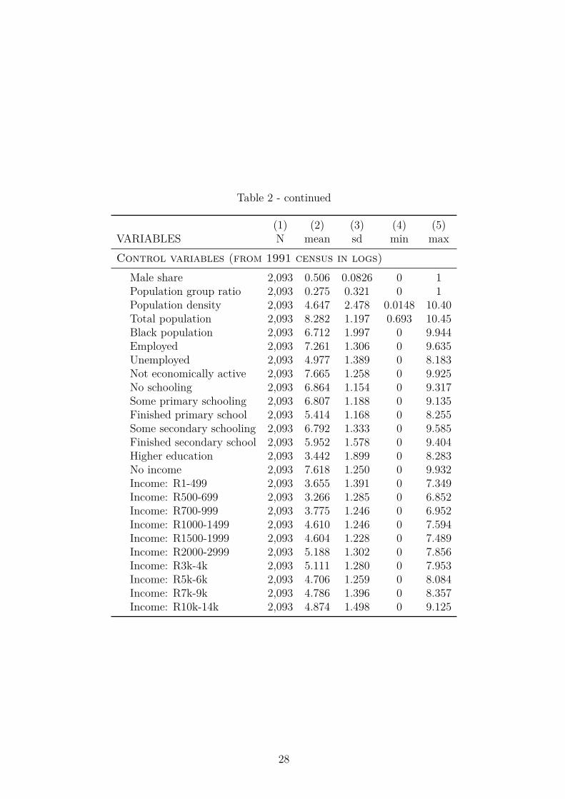
Table 2 - continued

(1) (2) (3) (4) (5)VARIABLES N mean sd min maxControl variables (from 1991 census in logs)

Male share 2,093 0.506 0.0826 0 1Population group ratio 2,093 0.275 0.321 0 1Population density 2,093 4.647 2.478 0.0148 10.40Total population 2,093 8.282 1.197 0.693 10.45Black population 2,093 6.712 1.997 0 9.944Employed 2,093 7.261 1.306 0 9.635Unemployed 2,093 4.977 1.389 0 8.183Not economically active 2,093 7.665 1.258 0 9.925No schooling 2,093 6.864 1.154 0 9.317Some primary schooling 2,093 6.807 1.188 0 9.135Finished primary school 2,093 5.414 1.168 0 8.255Some secondary schooling 2,093 6.792 1.333 0 9.585Finished secondary school 2,093 5.952 1.578 0 9.404Higher education 2,093 3.442 1.899 0 8.283No income 2,093 7.618 1.250 0 9.932Income: R1-499 2,093 3.655 1.391 0 7.349Income: R500-699 2,093 3.266 1.285 0 6.852Income: R700-999 2,093 3.775 1.246 0 6.952Income: R1000-1499 2,093 4.610 1.246 0 7.594Income: R1500-1999 2,093 4.604 1.228 0 7.489Income: R2000-2999 2,093 5.188 1.302 0 7.856Income: R3k-4k 2,093 5.111 1.280 0 7.953Income: R5k-6k 2,093 4.706 1.259 0 8.084Income: R7k-9k 2,093 4.786 1.396 0 8.357Income: R10k-14k 2,093 4.874 1.498 0 9.125

28

Table 3: OLS and 2SLS baseline regressions

(1) (2) (3) (4)OLS 2SLS

Population growth Nonblack growth Population growth Nonblack growth

Panel A: Population growth rates (1991-1996)∆Black Population 1.126 0.127 0.360 -0.640

(0.0814) (0.0815) (0.862) (0.862)FS AP F-Stat - - 2.52 2.52

Panel B: Population growth rates (1991-2001)∆Black Population 0.899∗ -0.101∗ 1.061 0.0614

(0.0393) (0.0393) (0.115) (0.115)FS AP F-Stat - - 29.98 29.98

Panel C: Population growth rates (1991-2011)∆Black Population 0.895∗∗∗ -0.105∗∗∗ 0.993 -0.00709

(0.0236) (0.0236) (0.0873) (0.0873)FS AP F-Stat - - 42.95 42.95

Province fixed effects Yes Yes Yes Yes

Controls Yes Yes Yes Yes

Observations 2093 2093 2093 2093

Notes. This Table displays estimates of equation (2) in the text. Each cell presents estimates from aseparate regression. The baseline sample consists of all wards inside South Africa for which 1991 data isavailable. The standard errors are clustered on the municipality level. There are 201 clusters. Columns(1) and (2) are estimated using OLS and columns (3) and (4) are estimated using 2SLS where the naturallog of distance to the nearest homeland is used to instrument for absolute black population growth inthe relevant time period divided by the overall population. The outcome variable is absolute overall ornon-black population growth in the relevant time period divided by overall population. The relevanttime periods are 1991-1996 in Panel A, 1991-2001 in Panel B and 1991-2011 in Panel C. Controls includevariables on education, income, population group, population density and employment in 1991. There arenine provinces for which fixed effects are included. The estimated coefficients for the first stage regressionsare reported in the appendix. Coefficients that are significantly different from zero at the 90% level ofconfidence are marked with a *; at the 95% level, a **; and at the 99% level, a *** in columns (2) and(4). In columns (1) and (3) they denote statistical significant departures from one. Standard errors inparentheses.

29

Table 4: 2SLS regressions using different sub-samples

(1) (2) (3) (4) (5) (6) (7)Dummy for

Johannesburg Drop within 10 km Drop < 5% white Drop < 10% white Drop distance ≥ 6 Districtfixed effects

Municipalitylevel

Panel A: Population growth rates (1991-1996)∆Black Population -0.640 -0.385 22.37 19.75 -0.655 -1.652 -0.174∗∗∗

(0.861) (0.442) (32.85) (25.53) (0.853) (1.926) (0.0576)FS AP F-Stat 2.52 1.36 0.25 0.31 2.61 1.67 10.27

Panel B: Population growth rates (1991-2001)∆Black Population 0.0688 0.0661 0.170 0.231 0.00799 -0.0392 0.0379

(0.112) (0.189) (0.144) (0.173) (0.108) (0.0837) (0.154)FS AP F-Stat 32.23 12.51 30.67 25.55 30.55 34.68 11.17

Panel C: Population growth rates (1991-2011)∆Black Population -0.00019 0.0460 0.0486 0.0618 -0.0747 -0.119 -0.0742

(0.0857) (0.131) (0.139) (0.146) (0.0879) (0.0771) (0.151)FS AP F-Stat 44.67 20.69 31.09 28.89 42.81 36.59 12.91

District fixed effects No No No No No Yes No

Province fixed effects Yes Yes Yes Yes Yes No Yes

Controls Yes Yes Yes Yes Yes Yes Yes

Observations 2093 1790 1374 1137 1730 2093 203

Notes. This Table displays estimates of equation (2) in the text for different sub-samples. Column headings denote sub-sample used in each specification.Each cell presents estimates from a separate regression. The standard errors are clustered on the municipality level. There are 201 clusters. All columns areestimated using 2SLS where the natural log of distance to the nearest homeland is used to instrument for absolute black population growth in the relevanttime period divided by the overall population. The outcome variable is absolute non-black population growth in the relevant time period divided by the overallpopulation. The relevant time periods are 1991-1996 in Panel A, 1991-2001 in Panel B and 1991-2011 in Panel C. Controls include variables on education,income, population group, population density and employment in 1991. There are nine provinces for which fixed effects are included. The estimated coefficientsfor the first stage regressions are reported in the appendix. Coefficients that are significantly different from zero at the 90% level of confidence are marked witha *; at the 95% level, a **; and at the 99% level, a ***. 95% confidence intervals are in brackets.

30

Figure 4: The effect of initial density and size of shock for populationgrowth

This figure displays the βj,k coefficients resulting from estimating equation (3) in the main text.The size of the shock increases along the x-axis. It starts off with the highest decile of the distancedistribution going to the decile with the lowest values (i.e. those closest to a homeland). Similarly,the first value on the y-axis corresponds to those wards in the lowest decile of the initial populationdensity distribution while the last one contains the highest decile. The z-axis displays differences inthe conditional mean of non-black population growth in the period 1991-2011.

31

Table 5: Heterogeneity with respect to the initial population densityand level of urbanisation

(1) (2)High population density

dummyHigh urban share

dummy

Panel A: Population growth rates (1991-1996)∆Black Population -0.897 -7.333

(1.425) (11.35)High initial urban share dummy × 7.589∆Black Population (11.56)High initial population density dummy × 0.509∆Black Population (1.133)

FS AP F-Stat: ∆Black Population 0.81 0.07FS AP F-Stat: Urban interaction - 0.07FS AP F-Stat: Density interaction 0.45 -

Panel B: Population growth rates (1991-2001)∆Black Population 0.106 0.00167

(0.138) (0.111)High initial urban share dummy × 0.178∗∗

∆Black Population (0.0840)High initial population density dummy × 0.681∗∗

∆Black Population (0.284)


Panel C: Population growth rates (1991-2011)∆Black Population -0.0432 -0.0138

(0.0924) (0.0827)High initial urban share dummy × 0.0399∆Black Population (0.0619)High initial population density dummy × 0.348∗∗

∆Black Population (0.152)


Province fixed effects Yes Yes

Controls Yes Yes

Observations 2093 2093

Notes. This Table displays estimates of equation (2) in the text with anadditional interaction term. Each column displays one specification. Thestandard errors are clustered on the municipality level. There are 201 clusters.All columns are estimated using 2SLS. Absolute black population growth dividedby the overall population and the same term interacted with a dummy for highpopulation density in 1991 or for high urban share of households are theendogenous variables. Log distance to the nearest homeland and log distance tothe nearest homeland times a dummy for high population density in 1991 or highurban share of households are used as instruments for the endogenous variables.An area is defined as having a high initial population density if it is among the25% most dense areas. An area is defined as having a high urban share if itis among the areas with the 75% highest share of urban households in 1991.The outcome variable is absolute non-black population growth in the relevanttime period divided by the overall population. The relevant time periods are1991-1996 in Panel A, 1991-2001 in Panel B and 1991-2011 in Panel C. Controlsinclude variables on education, income, population group, population densityand employment in 1991. There are nine provinces for which fixed effects areincluded. The estimated coefficients for the first stage regressions are reportedin the appendix. Coefficients that are significantly different from zero at the90% level of confidence are marked with a *; at the 95% level, a **; and at the99% level, a ***. 95% confidence intervals are in brackets.

32

Figure 5: Missing wards

All wards are hollow. Those areas with red borders and fill are missing. The former homelands aregreen.

33

Table 6: Summary of first stage regressions for the baseline specificationswith different fixed effects

(1) (2) (3) (4)No FE Province FE District FE Municipality FE

Panel A: Population growth rates (1991-1996)log distance 0.308 -0.940 -0.936 -1.148

(0.365) (0.593) (0.723) (0.993)

Panel B: Population growth rates (1991-2001)log distance -0.00733∗∗∗ -0.00675∗∗∗ -0.00647∗∗∗ -0.00323∗∗

(0.000811) (0.00123) (0.00110) (0.00144)

Panel C: Population growth rates (1991-2011)log distance -0.00423∗∗∗ -0.00354∗∗∗ -0.00381∗∗∗ -0.00172∗∗

(0.000398) (0.000540) (0.000629) (0.000737)Level ofFixed effects

No Province District Municipality


Observations 2093 2093 2093 2093

Notes. This Table displays estimates of equation (1) in the main text. Col-umn headings denote different specification. Each cell presents estimatesfrom a separate regression. The standard errors are clustered on the munici-pality level. There are 201 clusters. All columns are estimated using OLSwhere the natural log of distance to the nearest homeland is the variable ofinterest. The outcome variable is absolute black population growth in therelevant time period divided by the overall population. The relevant timeperiods are 1991-1996 in Panel A, 1991-2001 in Panel B and 1991-2011 inPanel C. Controls include variables on education, income, population group,population density and employment in 1991. Fixed effects at varying levelsare included. The estimated coefficients for the first stage regressions arereported in the appendix. Coefficients that are statistically significant at the90% level of confidence are marked with a *; at the 95% level, a **; and atthe 99% level, a ***. Standard errors in parentheses.

34

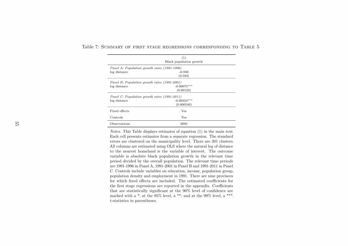
Table 7: Summary of first stage regressions corresponding to Table 5

(1)Black population growth

Panel A: Population growth rates (1991-1996)log distance -0.940

(0.593)

Panel B: Population growth rates (1991-2001)log distance -0.00675∗∗∗

(0.00123)

Panel C: Population growth rates (1991-2011)log distance -0.00354∗∗∗

(0.000540)

Fixed effects Yes

Controls Yes

Observations 2093

Notes. This Table displays estimates of equation (1) in the main text.Each cell presents estimates from a separate regression. The standarderrors are clustered on the municipality level. There are 201 clusters.All columns are estimated using OLS where the natural log of distanceto the nearest homeland is the variable of interest. The outcomevariable is absolute black population growth in the relevant timeperiod divided by the overall population. The relevant time periodsare 1991-1996 in Panel A, 1991-2001 in Panel B and 1991-2011 in PanelC. Controls include variables on education, income, population group,population density and employment in 1991. There are nine provincesfor which fixed effects are included. The estimated coefficients forthe first stage regressions are reported in the appendix. Coefficientsthat are statistically significant at the 90% level of confidence aremarked with a *; at the 95% level, a **; and at the 99% level, a ***.t-statistics in parentheses.

35

Table 8: Summary of first stage regressions corresponding to Table 6

(1) (2) (3) (4) (5) (6) (7)Dummy forJohannesburg Drop within 10 km Drop < 5% white Drop < 10% white Drop distance ≥ 6 District

fixed effectsMunicipalitylevel

Panel A: Population growth rates (1991-1996)log distance -0.947 -0.805 0.0758 0.106 -1.004 -0.936 -0.948

(0.597) (0.689) (0.152) (0.189) (0.622) (0.723) (0.700)

Panel B: Population growth rates (1991-2001)log distance -0.00697∗∗∗ -0.00625∗∗∗ -0.00777∗∗∗ -0.00747∗∗∗ -0.00693∗∗∗ -0.00647∗∗∗ -0.00602∗∗∗

(0.00123) (0.00177) (0.00140) (0.00148) (0.00125) (0.00110) (0.00137)

Panel C: Population growth rates (1991-2011)log distance -0.00367∗∗∗ -0.00395∗∗∗ -0.00345∗∗∗ -0.00359∗∗∗ -0.00345∗∗∗ -0.00381∗∗∗ -0.00316∗∗∗

(0.000550) (0.000868) (0.000619) (0.000668) (0.000527) (0.000629) (0.0005)Level ofFixed effects

Province Province Province Province Province District Province

Controls Yes Yes Yes Yes Yes Yes Yes

Observations 2093 1790 1374 1137 1730 2093 203

Notes. This Table displays estimates of equation (1) in the main text. Column headings denote different specification. Each cell presents estimatesfrom a separate regression. The standard errors are clustered on the municipality level. There are 201 clusters. All columns are estimated using OLSwhere the natural log of distance to the nearest homeland is the variable of interest. The outcome variable is absolute black population growth in therelevant time period divided by the overall population. The relevant time periods are 1991-1996 in Panel A, 1991-2001 in Panel B and 1991-2011 inPanel C. Controls include variables on education, income, population group, population density and employment in 1991. There are nine provincesfor which fixed effects are included. The estimated coefficients for the first stage regressions are reported in the appendix. Coefficients that arestatistically significant at the 90% level of confidence are marked with a *; at the 95% level, a **; and at the 99% level, a ***. Standard errors inparentheses.

36

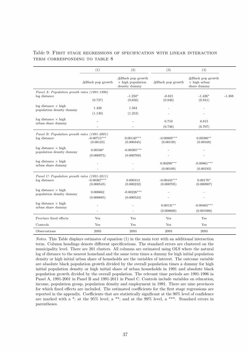
Table 9: First stage regressions of specification with linear interactionterm corresponding to table 8

(1) (2) (3) (4)

∆Black pop growth∆Black pop growth× high populationdensity dummy

∆Black pop growth∆Black pop growth× high urbanshare dummy

Panel A: Population growth rates (1991-1996)log distance -1.250∗ -0.821 -1.426∗ -1.388

(0.727) (0.656) (0.846) (0.841)

log distance × highpopulation density dummy 1.426 1.564 - -

(1.130) (1.253) - -

log distance × highurban share dummy - - 0.710 0.815

- - (0.736) (0.707)

Panel B: Population growth rates (1991-2001)log distance -0.00715∗∗∗ 0.00140∗∗∗ -0.00869∗∗∗ 0.00386∗∗

(0.00123) (0.000345) (0.00139) (0.00168)

log distance × highpopulation density dummy 0.00166∗ -0.00365∗∗∗ - -

(0.000975) (0.000769) - -

log distance × highurban share dummy - - 0.00290∗∗∗ -0.00861∗∗∗

- - (0.00109) (0.00193)

Panel C: Population growth rates (1991-2011)log distance -0.00367∗∗∗ 0.000312 -0.00445∗∗∗ 0.00176∗

(0.000545) (0.000232) (0.000705) (0.000907)

log distance × highpopulation density dummy 0.000662 -0.00226∗∗∗ - -

(0.000685) (0.000524) - -

log distance × highurban share dummy - - 0.00131∗∗ -0.00465∗∗∗

- - (0.000600) (0.001000)

Province fixed effects Yes Yes Yes Yes


Observations 2093 2093 2093 2093

Notes. This Table displays estimates of equation (1) in the main text with an additional interactionterm. Column headings denote different specifications. The standard errors are clustered on themunicipality level. There are 201 clusters. All columns are estimated using OLS where the naturallog of distance to the nearest homeland and the same term times a dummy for high initial populationdensity or high initial urban share of households are the variables of interest. The outcome variableare absolute black population growth divided by the overall population times a dummy for highinitial population density or high initial share of urban households in 1991 and absolute blackpopulation growth divided by the overall population. The relevant time periods are 1991-1996 inPanel A, 1991-2001 in Panel B and 1991-2011 in Panel C. Controls include variables on education,income, population group, population density and employment in 1991. There are nine provincesfor which fixed effects are included. The estimated coefficients for the first stage regressions arereported in the appendix. Coefficients that are statistically significant at the 90% level of confidenceare marked with a *; at the 95% level, a **; and at the 99% level, a ***. Standard errors inparentheses.

37

Migration and Urbanisation in Post-Apartheid South …ftp.iza.org/dp10113.pdf · Migration and...

Documents

Transcript of Migration and Urbanisation in Post-Apartheid South …ftp.iza.org/dp10113.pdf · Migration and...