Middle East Technical University Department of Mechanical...

Middle East Technical University

Department of Mechanical Engineering

ME 413 Introduction to Finite Element Analysis

Chapter 4

Trusses, Beams and Frames

These notes are prepared by

Dr. Cüneyt Sert

http://www.me.metu.edu.tr/people/cuneyt

[email protected]

These notes are prepared with the hope to be useful to those who want to learn and teach FEM. You are free to use them. Please send feedbacks to the above email address.

4-1

What Is This Chapter About?

• We’ll study FEM formulations of

• deformation of planar trusses

• bending of beams

• deformation of frames (as the superposition of planar truss and beam formulations)

• These problems will be studied as 1D, but there will be multiple unknowns at a node.

• We’ll modify the 1D FEM code to solve these problems.

METU – Dept. of Mechanical Engineering – ME 413 Int. to Finite Element Analysis – Lecture Notes of Dr. Sert 4-2

Deformation of a Bar

• A bar is a structural member that is loaded axially.

• It is either in direct tension or compression.

• Axial deformation, 𝑢, is governed by the following DE

−𝑑

𝑑𝑥𝐸𝐴𝑑𝑢

𝑑𝑥= 0

solution of which is linear for constant 𝐸 and 𝐴.

• Even a single linear element can solve this problem exactly.


𝐹 𝐸, 𝐴

𝑥

Deformation of a Bar (cont’d)

• Elemental weak form of the problem is

𝐸𝐴𝑑𝑢

𝑑𝑥

𝑑𝑤

𝑑𝑥 𝑑𝑥

Ω𝑒 = 𝑤𝐸𝐴

𝑑𝑢

𝑑𝑥𝑥2𝑒

𝑄2𝑒

+ −𝑤𝐸𝐴𝑑𝑢

𝑑𝑥𝑥1𝑒

𝑄1𝑒

• SV of the problem is the axial force : 𝐸𝐴𝑑𝑢

𝑑𝑥𝑛𝑥

• Elemental stiffness matrix is

• Elemental system is


𝐾𝑖𝑗𝑒 = 𝐸𝐴

𝑑𝑆𝑖𝑑𝜉

1

𝐽𝑒 𝑑𝑆𝑗

𝑑𝜉

1

𝐽𝑒 𝐽𝑒𝑑𝜉

Ω𝑒

𝐸𝐴

ℎ𝑒1 −1−1 1

𝑢1𝑒

𝑢2𝑒 =

𝑄1𝑒

𝑄2𝑒

Elemental force vector is zero

• A truss consists of several bars connected with frictionless pin joints.

• Note that this is not the actual meaning of truss in civil engineering.

• Each member can only carry axial force, but no shear force or bending moment.

• All members of a planar truss lie on a 2D plane. Space truss is the 3D version.

• A truss can be loaded with multiple point forces at its joints.

• Typically there is at least one fixed joint.

• Some joints might have restricted motion.

• Deformations are small, i.e. general shape of the truss is similar before and after loading.

Planar Truss


𝐹1

𝐹2

• Each member of a truss can be treated as an element of a FE mesh.

• The elemental system derived previously for a bar is valid for each member.

• But in order to be able to use it, different coordinate systems aligned with each member should be used. These local coordinates are shown below with 𝑥 1 and 𝑥 2.

Planar Truss – Local Coordinates


e=1

𝑥 1

𝑄 11

𝑄 21

𝐸𝐴

ℎ11 −1−1 1

𝑢 11

𝑢 21 =

𝑄 11

𝑄 21

Nodal deflections of e=1 in 𝑥 1 direction

Nodal forces of e=1 in 𝑥 1 direction

For the 1st member

1

2 e=2

𝑥 2

𝑄 12 𝑄 2

2

𝐸𝐴

ℎ21 −1−1 1

𝑢 12

𝑢 22 =

𝑄 12

𝑄 22

Nodal deflections of e=2 in 𝑥 2 direction

Nodal forces of e=2 in 𝑥 2 direction

For the 2nd member

1 2

• During the assembly of the elemental systems, PVs and SVs written for a common 𝑥𝑦 coordinate system should be used.

• For each element a transformation between local 𝑥 coordinate and the global 𝑥𝑦 coordinates is necessary.

• This is a purely geometrical transformation.

Planar Truss – Transformation Matrix


𝑢1𝑥𝑒 = 𝑢 1

𝑒 cos (𝜃𝑒)

𝑢1𝑦𝑒 = 𝑢 1

𝑒 sin (𝜃𝑒)

Multiply the 1st eqn with cos (𝜃𝑒) and the 2nd eqn with sin 𝜃𝑒 and add them up.

𝑢1𝑥𝑒 cos 𝜃𝑒 + 𝑢1𝑦

𝑒 sin 𝜃𝑒 = 𝑢 1𝑒 cos2 𝜃𝑒 + sin2 𝜃𝑒

1

𝑢 1𝑒 = 𝑢1𝑥

𝑒 cos 𝜃𝑒 + 𝑢1𝑦𝑒 sin 𝜃𝑒

e

𝑥 𝑒

𝑢 1𝑒

𝜃𝑒

𝑄 1𝑒

𝑢 2𝑒

𝑄 2𝑒

𝑥

𝑦 𝑢1𝑦𝑒

𝑢1𝑥𝑒 𝑄1𝑦

𝑒

𝑄1𝑥𝑒

𝑢2𝑦𝑒

𝑢2𝑥𝑒

𝑄2𝑦𝑒

𝑄2𝑥𝑒

1

2

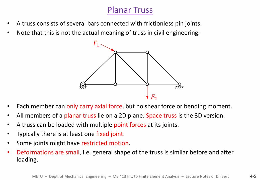
• Similary for the 2nd node of element e : 𝑢 2𝑒 = 𝑢2𝑥

𝑒 cos 𝜃𝑒 + 𝑢2𝑦𝑒 sin 𝜃𝑒

• Together these two eqns become

𝑢 1𝑒

𝑢 2𝑒 =cos (𝜃𝑒) sin(𝜃𝑒) 0 0

0 0 cos (𝜃𝑒) sin(𝜃𝑒)

𝑢1𝑥𝑒

𝑢1𝑦𝑒

𝑢2𝑥𝑒

𝑢2𝑦𝑒

𝑢 𝑒 = [𝑇𝑒] Δ𝑒

• A similar eqn can be written for the SVs too

𝑄 𝑒 = [𝑇𝑒] 𝑄𝑒


Transformation matrix, [𝑇𝑒]

Δ𝑒 includes both 𝑢𝑥𝑒’s and 𝑢𝑦

𝑒 ’s.

Each node has 2 unknowns and in total one element has 4 unknowns.

𝑄𝑒 = 𝑄1𝑥𝑒 𝑄1𝑦

𝑒 𝑄2𝑥𝑒 𝑄2𝑦

𝑒 𝑇

Planar Truss – Transformation Matrix (cont’d)

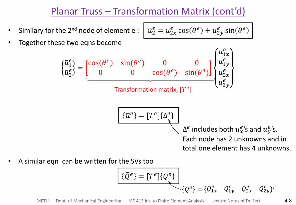
• [𝑇𝑒] can be used to transform the original 2x2 elemental system into a new 4x4 elemental system

• Original 2x2 elemental system using bars :

• Using 𝑢 𝑒 = [𝑇𝑒] Δ𝑒 and 𝑄 𝑒 = [𝑇𝑒] 𝑄𝑒

𝐾 𝑒 [𝑇𝑒] Δ𝑒 = [𝑇𝑒] 𝑄𝑒

• Premultiply this eqn by 𝑇𝑒 𝑇

𝑇𝑒 𝑇 𝐾 𝑒 [𝑇𝑒] Δ𝑒 = 𝑇𝑒 𝑇[𝑇𝑒] 𝑄𝑒


𝐸𝐴

ℎ𝑒1 −1−1 1

𝑢 1𝑒

𝑢 2𝑒 =

𝑄 1𝑒

𝑄 2𝑒

or 𝐾 𝑒 𝑢 𝑒 = {𝑄 𝑒}

𝐾𝑒 1

Planar Truss – [𝐾𝑒] Transformation Matrix

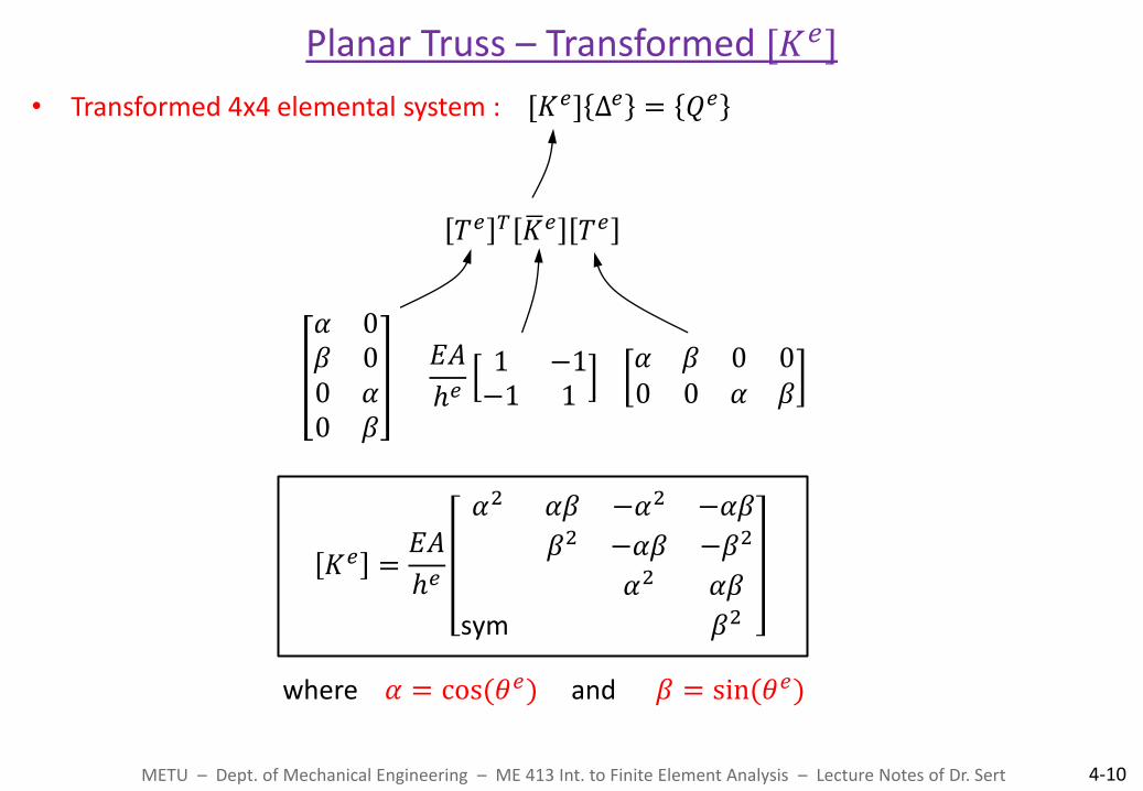
• Transformed 4x4 elemental system : [𝐾𝑒] Δ𝑒 = 𝑄𝑒


𝛼 0𝛽 00 𝛼0 𝛽

𝐸𝐴

ℎ𝑒1 −1−1 1

𝛼 𝛽 0 00 0 𝛼 𝛽

𝑇𝑒 𝑇 𝐾 𝑒 𝑇𝑒

𝐾𝑒 =𝐸𝐴

ℎ𝑒

𝛼2 𝛼𝛽 −𝛼2 −𝛼𝛽

𝛽2 −𝛼𝛽 −𝛽2

𝛼2 𝛼𝛽

sym 𝛽2

where 𝛼 = cos(𝜃𝑒) and 𝛽 = sin(𝜃𝑒)

Planar Truss – Transformed [𝐾𝑒]

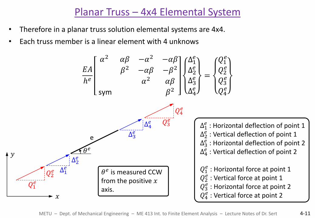
• Therefore in a planar truss solution elemental systems are 4x4.

• Each truss member is a linear element with 4 unknows

𝐸𝐴

ℎ𝑒

𝛼2 𝛼𝛽 −𝛼2 −𝛼𝛽

𝛽2 −𝛼𝛽 −𝛽2

𝛼2 𝛼𝛽

sym 𝛽2

Δ1𝑒

Δ2𝑒

Δ3𝑒

Δ4𝑒

=

𝑄1𝑒

𝑄2𝑒

𝑄3𝑒

𝑄4𝑒

Planar Truss – 4x4 Elemental System


e

𝜃𝑒

𝑥

𝑦 Δ2𝑒

Δ1𝑒 𝑄2

𝑒

𝑄1𝑒

Δ4𝑒

Δ3𝑒

𝑄4𝑒

𝑄3𝑒 Δ1

𝑒 : Horizontal deflection of point 1 Δ2𝑒 : Vertical deflection of point 1 Δ3𝑒 : Horizontal deflection of point 2 Δ4𝑒 : Vertical deflection of point 2

𝑄1𝑒 : Horizontal force at point 1 𝑄2𝑒 : Vertical force at point 1 𝑄3𝑒 : Horizontal force at point 2 𝑄4𝑒 : Vertical force at point 2

𝜃𝑒 is measured CCW from the positive 𝑥 axis.

• Consider the following truss problem.

• There are 𝑁𝐸 = 3 elements and 𝑁𝑁 = 3 nodes.

• At each node there are 𝑁𝑁𝑈 = 2 unknown deflections. Totally there are 𝑁𝑈 = 6 unknowns.

• 4 of these unknowns are known. Nodes 1 and 2 are fixed.

• We need to determine 2 deflections (horizontal and vertical) at node 3 and, if desired, the reaction forces at nodes 1 and 2.

Planar Truss – Local to Global Unknown Mapping


2𝑃

𝑃

1 2

3

e=1

e=2 e=3

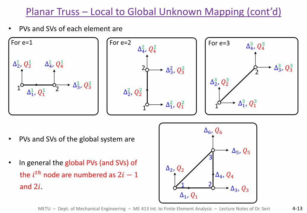
• PVs and SVs of each element are

• PVs and SVs of the global system are

• In general the global PVs (and SVs) of

the 𝑖𝑡ℎ node are numbered as 2𝑖 − 1

and 2𝑖.


1 2

3

Δ1, 𝑄1

Δ2, 𝑄2

Δ3, 𝑄3

Δ4, 𝑄4

Δ5, 𝑄5

Δ6, 𝑄6

Δ11 , 𝑄11

Δ31 , 𝑄31

Δ21 , 𝑄21 Δ4

1 , 𝑄41

For e=1

1 2

Δ12, 𝑄12

Δ32 , 𝑄32

Δ22 , 𝑄22

Δ42, 𝑄42

For e=2

1

2

Δ13, 𝑄13

Δ33 , 𝑄33

Δ23 , 𝑄23

Δ43 , 𝑄43 For e=3

1

2

Planar Truss – Local to Global Unknown Mapping (cont’d)

• Assembly process is about local-to- global unknown mapping for each element


Δ1 Δ2 Δ3 Δ4 Δ5 Δ6

= Δ Global unknowns

Unknowns of e=1 : Δ1 =

Δ11

Δ21

Δ31

Δ41


Δ12

Δ22

Δ32

Δ42


Δ13

Δ23

Δ33

Δ43

Planar Truss – Local to Global Unknown Mapping (cont’d)

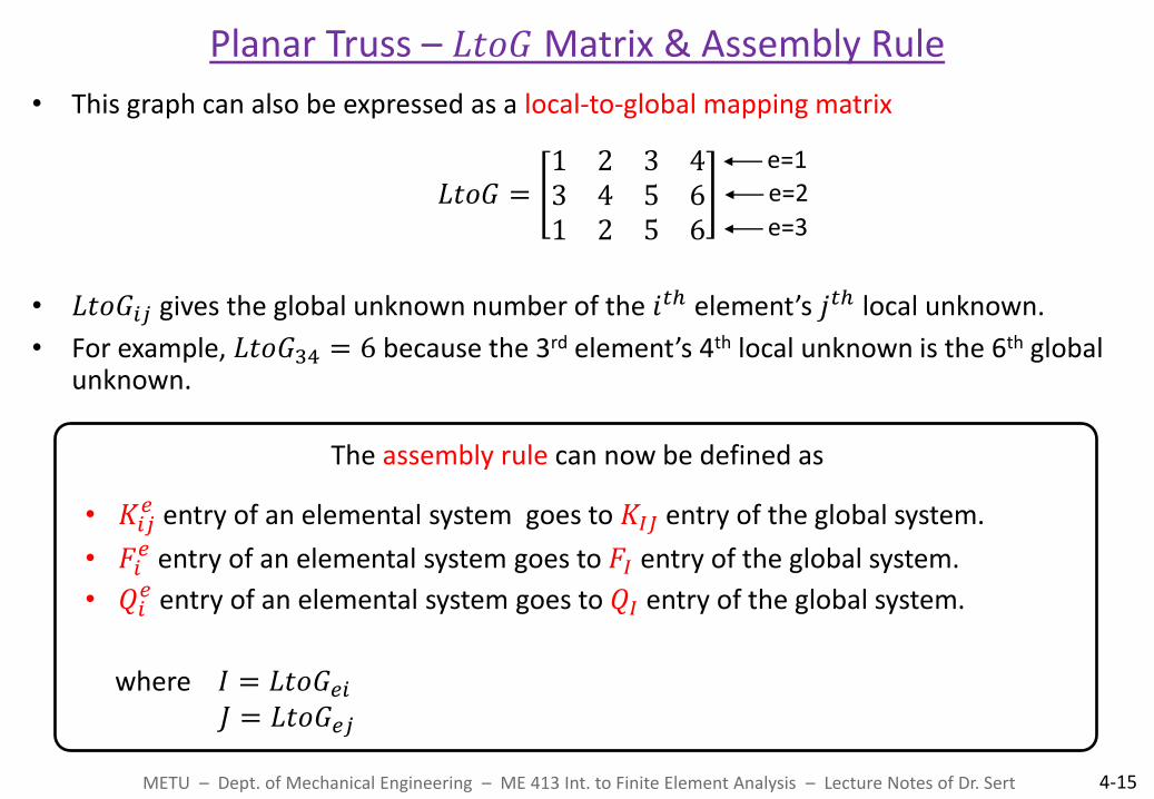
• This graph can also be expressed as a local-to-global mapping matrix

𝐿𝑡𝑜𝐺 =1 2 3 43 4 5 61 2 5 6

• 𝐿𝑡𝑜𝐺𝑖𝑗 gives the global unknown number of the 𝑖𝑡ℎ element’s 𝑗𝑡ℎ local unknown.

• For example, 𝐿𝑡𝑜𝐺34 = 6 because the 3rd element’s 4th local unknown is the 6th global unknown.

The assembly rule can now be defined as

• 𝐾𝑖𝑗𝑒 entry of an elemental system goes to 𝐾𝐼𝐽 entry of the global system.

• 𝐹𝑖𝑒 entry of an elemental system goes to 𝐹𝐼 entry of the global system.

• 𝑄𝑖𝑒 entry of an elemental system goes to 𝑄𝐼 entry of the global system.

where 𝐼 = 𝐿𝑡𝑜𝐺𝑒𝑖 𝐽 = 𝐿𝑡𝑜𝐺𝑒𝑗

Planar Truss – 𝐿𝑡𝑜𝐺 Matrix & Assembly Rule


e=1 e=2

e=3

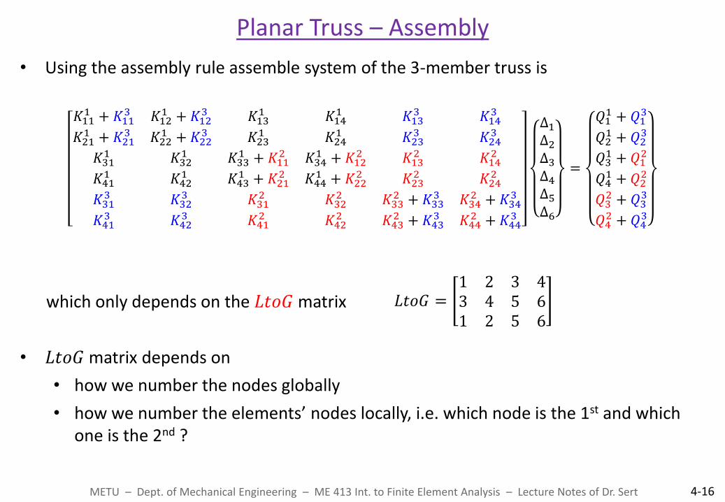
• Using the assembly rule assemble system of the 3-member truss is

𝐾111 + 𝐾11

3 𝐾121 + 𝐾12

3 𝐾131 𝐾14

1 𝐾133 𝐾14

3

𝐾211 + 𝐾21

3 𝐾221 + 𝐾22

3 𝐾231 𝐾24

1 𝐾233 𝐾24

3

𝐾311 𝐾32

1 𝐾331 + 𝐾11

2 𝐾341 + 𝐾12

2 𝐾132 𝐾14

2

𝐾411 𝐾42

1 𝐾431 + 𝐾21

2 𝐾441 + 𝐾22

2 𝐾232 𝐾24

2

𝐾313 𝐾32

3 𝐾312 𝐾32

2 𝐾332 + 𝐾33

3 𝐾342 + 𝐾34

3

𝐾413 𝐾42

3 𝐾412 𝐾42

2 𝐾432 + 𝐾43

3 𝐾442 + 𝐾44

3

Δ1Δ2Δ3Δ4Δ5Δ6

=

𝑄11 + 𝑄1

3

𝑄21 + 𝑄2

3

𝑄31 + 𝑄1

2

𝑄41 + 𝑄2

2

𝑄32 + 𝑄3

3

𝑄42 + 𝑄4

3

which only depends on the 𝐿𝑡𝑜𝐺 matrix

• 𝐿𝑡𝑜𝐺 matrix depends on

• how we number the nodes globally

• how we number the elements’ nodes locally, i.e. which node is the 1st and which one is the 2nd ?

Planar Truss – Assembly


𝐿𝑡𝑜𝐺 =1 2 3 43 4 5 61 2 5 6

• Consider the following truss problem with 2 point loads.

• How should we use the points loads?

• They are used in the boundary term vector.

• 𝑄 of this problem is

𝑄 =

𝑄1𝑄2𝑄3𝑄4𝑄5𝑄6

=

𝑄11 + 𝑄1

3

𝑄21 + 𝑄2

3

𝑄31 + 𝑄1

2

𝑄41 + 𝑄2

2

𝑄32 + 𝑄3

3

𝑄42 + 𝑄4

3

• If there is no horizontal (or vertical) force at a node, the corresponding SV is set to zero.

• If there is a given point load at a node, the corresponding SV is set to the given value.

• At supports SV(s) are unknown and can be calculated during post-processing.

• Be careful with the direction (sign) of forces.

Planar Truss – Point Loads


2𝑃

𝑃

1 2

3

e=1

e=2 e=3

𝑥

𝑦

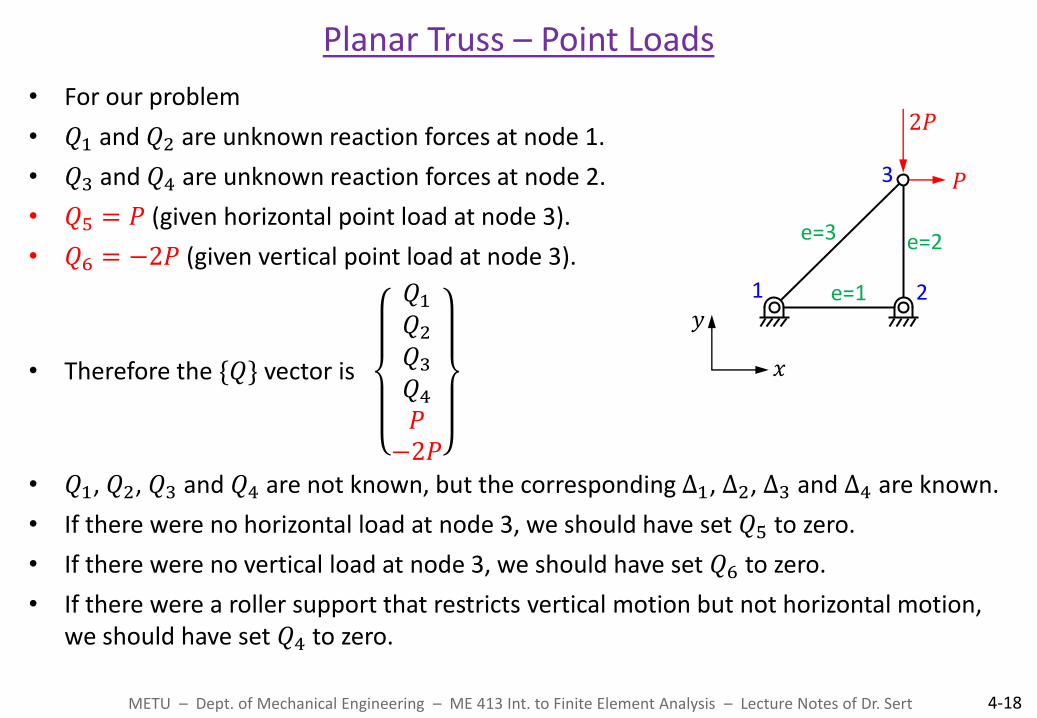
• For our problem

• 𝑄1 and 𝑄2 are unknown reaction forces at node 1.

• 𝑄3 and 𝑄4 are unknown reaction forces at node 2.

• 𝑄5 = 𝑃 (given horizontal point load at node 3).

• 𝑄6 = −2𝑃 (given vertical point load at node 3).

• Therefore the {𝑄} vector is

𝑄1𝑄2𝑄3𝑄4𝑃−2𝑃

• 𝑄1, 𝑄2, 𝑄3 and 𝑄4 are not known, but the corresponding Δ1, Δ2, Δ3 and Δ4 are known.

• If there were no horizontal load at node 3, we should have set 𝑄5 to zero.

• If there were no vertical load at node 3, we should have set 𝑄6 to zero.

• If there were a roller support that restricts vertical motion but not horizontal motion, we should have set 𝑄4 to zero.

Planar Truss – Point Loads


2𝑃

𝑃

1 2

3

e=1

e=2 e=3

𝑥

𝑦

Example 4.1


Example 4.1 : Solve the following truss problem.

• Find the deflection of the nodes.

• Determine the forces and stresses in each member.

• Determine the reaction forces at the supports.

𝐸 and 𝐴 values are the same for each member.

e.g.

2𝑃

𝑃

1 2

3

e=1

e=2 e=3

𝐿

𝐿

Example 4.1 (cont’d)


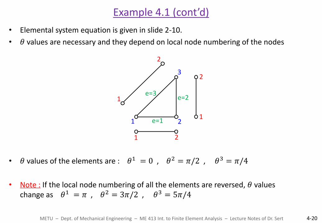
• Elemental system equation is given in slide 2-10.

• 𝜃 values are necessary and they depend on local node numbering of the nodes

• 𝜃 values of the elements are : 𝜃1 = 0 , 𝜃2 = 𝜋/2 , 𝜃3 = 𝜋/4

• Note : If the local node numbering of all the elements are reversed, 𝜃 values change as 𝜃1 = 𝜋 , 𝜃2 = 3𝜋/2 , 𝜃3 = 5𝜋/4

1 2

3

e=1

e=2 e=3

1

2

1

2

1 2

• Elemental systems are

For e=1 :

For e=2 :

For e=3 :



𝛼 = cos 𝜃1 = 1 𝛽 = sin 𝜃1 = 0 ℎ1 = 𝐿

𝛼 = cos 𝜃2 = 0 𝛽 = sin 𝜃2 = 1 ℎ2 = 𝐿

𝛼 = cos 𝜃3 = 1/ 2

𝛽 = sin 𝜃3 = 1/ 2

ℎ3 = 2𝐿

→ 𝐾1 =𝐸𝐴

𝐿

1 0 −1 0 0 0 0 1 0 0

sym.

→ 𝐾2 =𝐸𝐴

𝐿

0 0 0 0 1 0 −1 0 0 1

sym.

→ 𝐾3 =𝐸𝐴

2 2𝐿

1 1 −1 −1 1 −1 −1 1 1 1

sym.

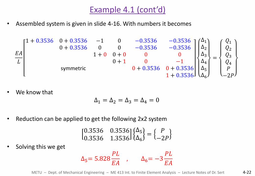
• Assembled system is given in slide 4-16. With numbers it becomes

𝐸𝐴

𝐿

1 + 0.3536 0 + 0.3536 −1 0 −0.3536 −0.3536 0 + 0.3536 0 0 −0.3536 −0.3536 1 + 0 0 + 0 0 0 0 + 1 0 −1 symmetric 0 + 0.3536 0 + 0.3536 1 + 0.3536

Δ1Δ2Δ3Δ4Δ5Δ6

=

𝑄1𝑄2𝑄3𝑄4𝑃−2𝑃

• We know that Δ1 = Δ2 = Δ3 = Δ4 = 0

• Reduction can be applied to get the following 2x2 system

0.3536 0.35360.3536 1.3536

∆5∆6=𝑃−2𝑃

• Solving this we get

∆5= 5.828𝑃𝐿

𝐸𝐴 , ∆6= −3

𝑃𝐿

𝐸𝐴



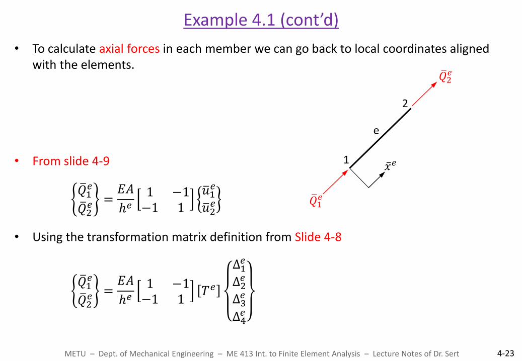
• To calculate axial forces in each member we can go back to local coordinates aligned with the elements.

• From slide 4-9

𝑄 1𝑒

𝑄 2𝑒 =𝐸𝐴

ℎ𝑒1 −1−1 1

𝑢 1𝑒

𝑢 2𝑒

• Using the transformation matrix definition from Slide 4-8

𝑄 1𝑒

𝑄 2𝑒 =𝐸𝐴

ℎ𝑒1 −1−1 1

𝑇𝑒

Δ1𝑒

Δ2𝑒

Δ3𝑒

Δ4𝑒



e

𝑥 𝑒

𝑄 1𝑒

𝑄 2𝑒

1

2

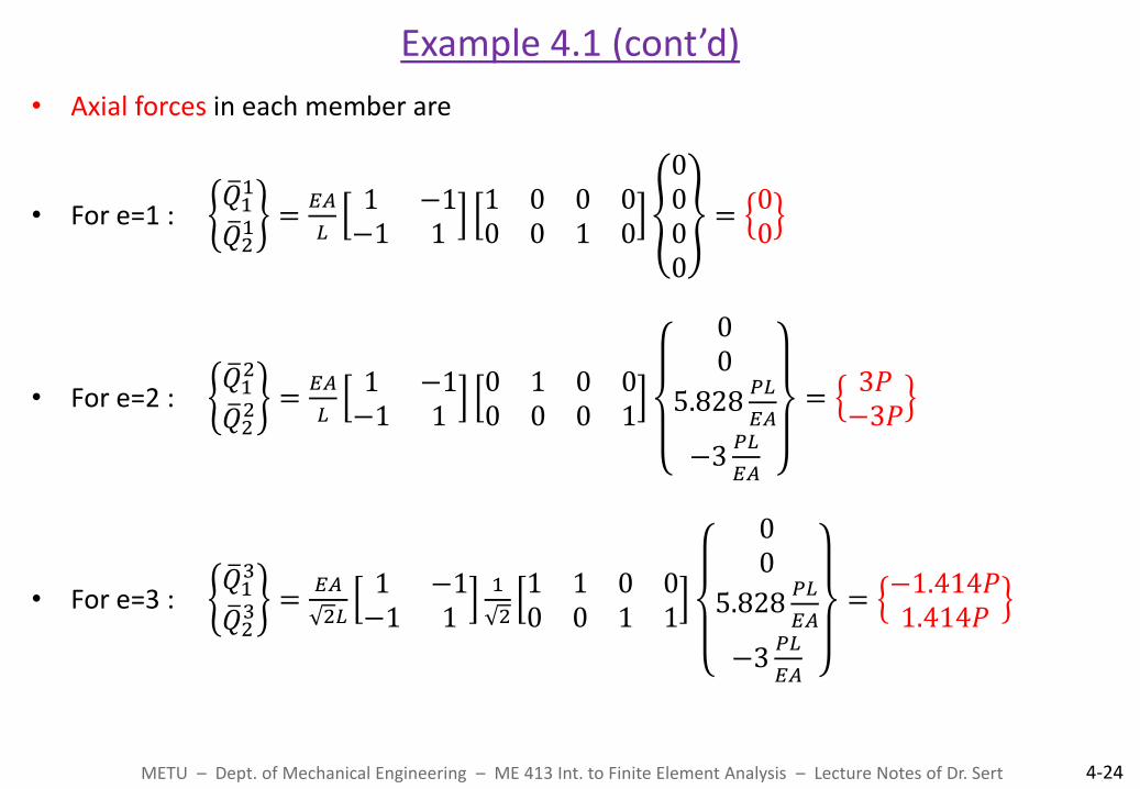
• Axial forces in each member are

• For e=1 : 𝑄 11

𝑄 21 =

𝐸𝐴

𝐿

1 −1−1 1

1 0 0 00 0 1 0

0000

=00

• For e=2 : 𝑄 12

𝑄 22 =

𝐸𝐴

𝐿

1 −1−1 1

0 1 0 00 0 0 1

00

5.828𝑃𝐿

𝐸𝐴

−3𝑃𝐿

𝐸𝐴

=3𝑃−3𝑃

• For e=3 : 𝑄 13

𝑄 23 =

𝐸𝐴

2𝐿

1 −1−1 1

1

2

1 1 0 00 0 1 1

00

5.828𝑃𝐿

𝐸𝐴

−3𝑃𝐿

𝐸𝐴

=−1.414𝑃1.414𝑃



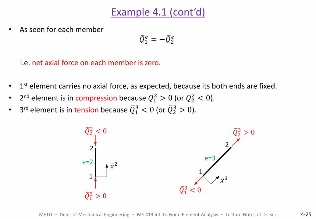
• As seen for each member 𝑄 1𝑒 = −𝑄 2

𝑒

i.e. net axial force on each member is zero.

• 1st element carries no axial force, as expected, because its both ends are fixed.

• 2nd element is in compression because 𝑄 12 > 0 (or 𝑄 2

2 < 0).

• 3rd element is in tension because 𝑄 13 < 0 (or 𝑄 2

3 > 0).



e=2

1

2

𝑄 12 > 0

𝑄 22 < 0

𝑥 2 e=3

1

2

𝑄 13 < 0

𝑄 23 > 0

𝑥 3

• Axial stresses in each element can be calculated.

For e=1 : 𝜎1 =𝑄 21

𝐴= 0

For e=2 : 𝜎2 =𝑄 22

𝐴= −3

𝑃

𝐴 (Negative stress indicates compression)

For e=3 : 𝜎3 =𝑄 23

𝐴= 1.414

𝑃

𝐴 (Positive stress indicates tension)

• Finally forces at the supports can be calculated using the 6x6 system of Slide 4-22.

At node 1 : 𝑄1 =𝐸𝐴

𝐿1.3536∆1 + 0.3536∆2 − ∆3 − 0.3536∆5 − 0.3536∆6 = −𝑃

𝑄2 =𝐸𝐴

𝐿0.3536∆1 + 0.3536∆2 − 0.3536∆5 − 0.3536∆6 = −𝑃

At node 2 : 𝑄3 =𝐸𝐴

𝐿−∆1 + ∆3 = 0

𝑄4 =𝐸𝐴

𝐿∆4 − ∆6 = 3𝑃



𝑃

𝑃

3𝑃 Forces at the supports are the opposite of the calculated ones

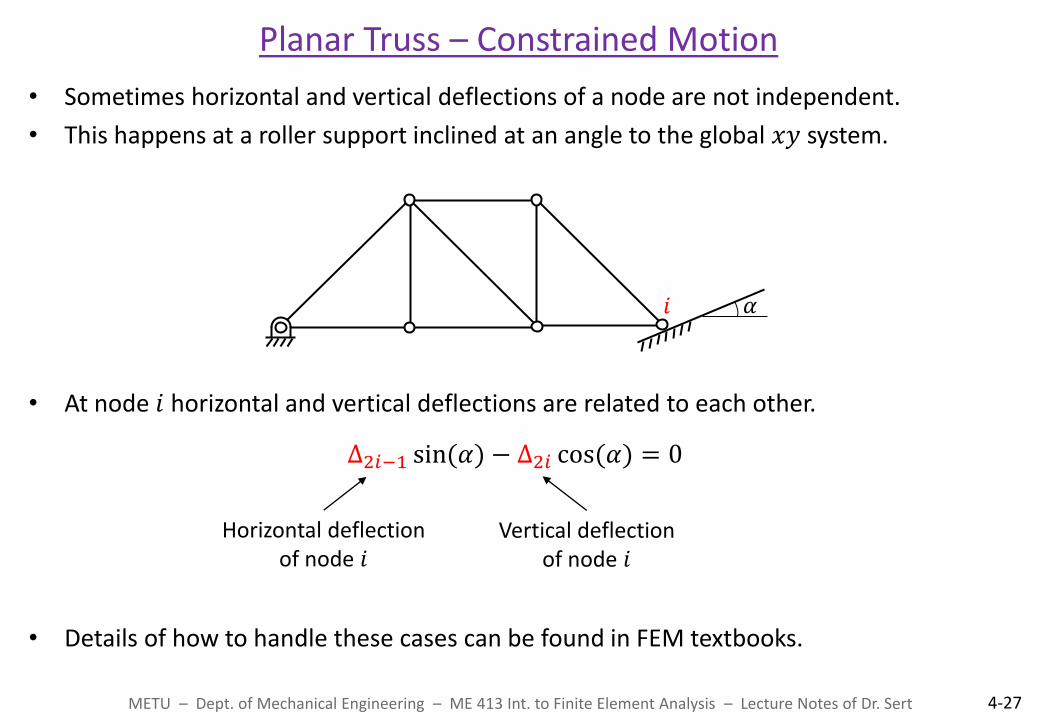
• Sometimes horizontal and vertical deflections of a node are not independent.

• This happens at a roller support inclined at an angle to the global 𝑥𝑦 system.

• At node 𝑖 horizontal and vertical deflections are related to each other.

∆2𝑖−1 sin(𝛼) − ∆2𝑖 cos(𝛼) = 0

• Details of how to handle these cases can be found in FEM textbooks.

Planar Truss – Constrained Motion


𝛼 𝑖

Horizontal deflection of node 𝑖

Vertical deflection of node 𝑖

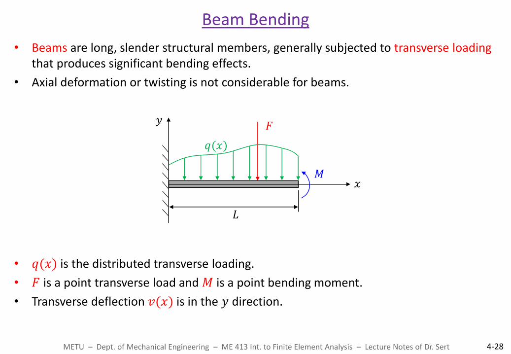
• Beams are long, slender structural members, generally subjected to transverse loading that produces significant bending effects.

• Axial deformation or twisting is not considerable for beams.

• 𝑞(𝑥) is the distributed transverse loading.

• 𝐹 is a point transverse load and 𝑀 is a point bending moment.

• Transverse deflection 𝑣(𝑥) is in the 𝑦 direction.

Beam Bending


𝑞(𝑥)

𝐿

𝑥

𝑦 𝐹

𝑀

• The assumption behind the Euler-Bernoulli beam theory is that plane cross sections perpendicular to the longitudinal axis of the beam before bending, remain perpendicular to the longitudional axis after bending.

• Governing DE is

• 𝑣(𝑥) : Unknown transverse deflection

• 𝑞(𝑥) : Known distributed transverse load

• 𝐸𝐼 : Known flexural rigidity of the beam, i.e. product of modulus of elasticity and the

second moment of inertia.

Euler-Bernoulli Beam Theory


𝑥 Before bending :

After bending :

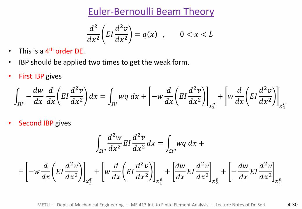
𝑑2

𝑑𝑥2𝐸𝐼𝑑2𝑣

𝑑𝑥2= 𝑞 𝑥 , 0 < 𝑥 < 𝐿

𝑑2


𝑑𝑥2= 𝑞 𝑥 , 0 < 𝑥 < 𝐿

• This is a 4th order DE.

• IBP should be applied two times to get the weak form.

• First IBP gives

−𝑑𝑤

𝑑𝑥 𝑑

𝑑𝑥𝐸𝐼𝑑2𝑣

𝑑𝑥2𝑑𝑥

Ω𝑒= 𝑤𝑞 𝑑𝑥

Ω𝑒+ −𝑤

𝑑


𝑑𝑥2𝑥2𝑒

+ 𝑤𝑑


𝑑𝑥2𝑥1𝑒

• Second IBP gives

𝑑2𝑤


𝑑𝑥2𝑑𝑥

Ω𝑒= 𝑤𝑞 𝑑𝑥

Ω𝑒+

+ −𝑤𝑑


𝑑𝑥2𝑥2𝑒

+ 𝑤𝑑


𝑑𝑥2𝑥1𝑒

+𝑑𝑤


𝑑𝑥2𝑥2𝑒

+ −𝑑𝑤


𝑑𝑥2𝑥1𝑒

Euler-Bernoulli Beam Theory


• There are two PVs Transverse deflection : 𝑣

Slope : 𝑑𝑣

𝑑𝑥

• There are two SVs

Shear force : 𝑑


𝑑𝑥2

Bending moment : 𝐸𝐼𝑑2𝑣

𝑑𝑥2

• Sign conventions are

• Deflection in +𝑦 direction (upward) is positive.

• CCW rotation of the beam corresponds to positive slope.

• Shear force in +𝑦 direction (upward) is positive.

• CCW moment (in +𝑧 direction) is positive.

Euler-Bernoulli Beam Theory (cont’d)


• 2 node beam element has 4 PVs and 4 SVs

Two Node Beam Element


2 1 e

Δ1𝑒

Δ2𝑒

Δ3𝑒

Δ4𝑒 Δ𝑒 =

Δ1𝑒

Δ2𝑒

Δ3𝑒

Δ4𝑒

Transverse deflection at node 1

Transverse deflection at node 2

Slope at node 1

Slope at node 2

2 1 e

𝑄1𝑒

𝑄2𝑒

𝑄3𝑒

𝑄4𝑒 𝑄𝑒 =

𝑄1𝑒

𝑄2𝑒

𝑄3𝑒

𝑄4𝑒

Shear force at node 1

Shear force at node 2

Bending moment at node 1

Bending moment at node 2

• Weak form of the problem contains 2nd derivative of the transverse deflection.

• Not only the transverse deflection, but also its first derivative, i.e. slope should be continuous, because slope is a PV too.

• Over each element FE solution is

𝑣𝑒 = 𝑆𝑗 Δ𝑗𝑒

4

𝑗=1

• A 𝐶0 continuous solution for Δ𝑒 is NOT enough. It should be at least 𝐶1 continuous.

• Lagrange type shape functions used previously are not suitable.

• Hermite type shape functions should be used.

Hermite Type Shape Functions


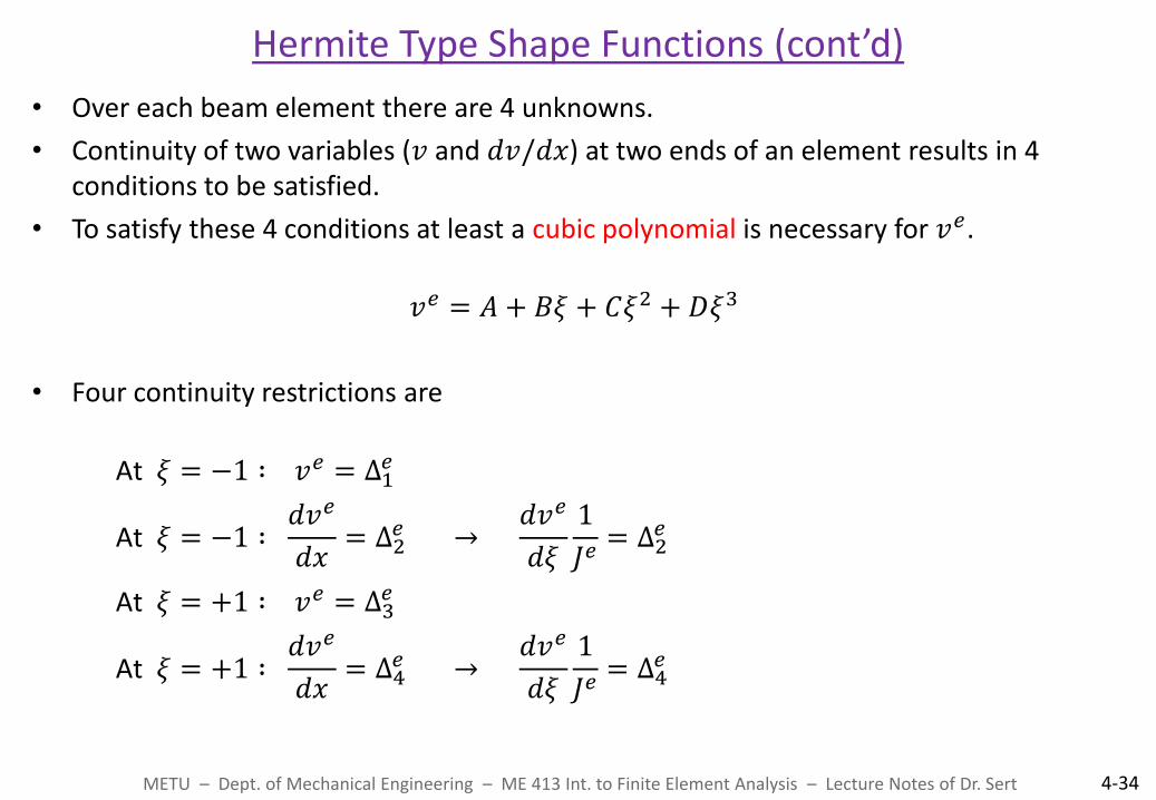
• Over each beam element there are 4 unknowns.

• Continuity of two variables (𝑣 and 𝑑𝑣/𝑑𝑥) at two ends of an element results in 4 conditions to be satisfied.

• To satisfy these 4 conditions at least a cubic polynomial is necessary for 𝑣𝑒.

𝑣𝑒 = 𝐴 + 𝐵𝜉 + 𝐶𝜉2 + 𝐷𝜉3

• Four continuity restrictions are

At 𝜉 = −1 ∶ 𝑣𝑒 = Δ1

𝑒

At 𝜉 = −1 ∶ 𝑑𝑣𝑒

𝑑𝑥= Δ2𝑒 →

𝑑𝑣𝑒

𝑑𝜉

1

𝐽𝑒= Δ2𝑒

At 𝜉 = +1 ∶ 𝑣𝑒 = Δ3𝑒

At 𝜉 = +1 ∶ 𝑑𝑣𝑒

𝑑𝑥= Δ4𝑒 →

𝑑𝑣𝑒

𝑑𝜉

1

𝐽𝑒= Δ4𝑒

Hermite Type Shape Functions (cont’d)


• Using 𝐽𝑒 these 4 conditions become

Δ1𝑒 = 𝐴 − 𝐵 + 𝐶 − 𝐷

Δ2𝑒 = 𝐵 − 2𝐶 + 3𝐷

2

ℎ𝑒

Δ3𝑒 = 𝐴 + 𝐵 + 𝐶 + 𝐷

Δ4𝑒 = 𝐵 + 2𝐶 + 3𝐷

2

ℎ𝑒

• Solve for 𝐴, 𝐵, 𝐶 and 𝐷 in terms of Δ1𝑒 , Δ2𝑒 , Δ3𝑒 and Δ4

𝑒 .

• Substitute them into the following equation

𝑆𝑗 Δ𝑗𝑒

4

𝑗=1

= 𝐴 + 𝐵𝜉 + 𝐶𝜉2 + 𝐷𝜉3

• And identify the 4 Hermite type cubic shape functions.



𝑣𝑒 𝑣𝑒

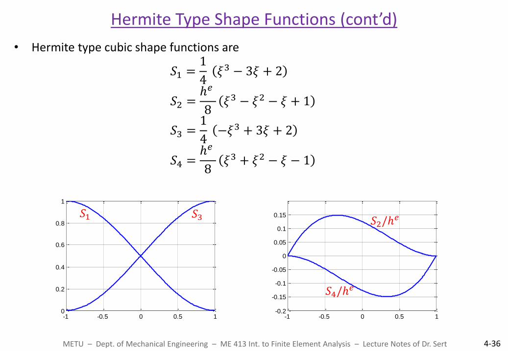
• Hermite type cubic shape functions are

𝑆1 =1

4 𝜉3 − 3𝜉 + 2

𝑆2 =ℎ𝑒

8𝜉3 − 𝜉2 − 𝜉 + 1

𝑆3 =1

4 −𝜉3 + 3𝜉 + 2

𝑆4 =ℎ𝑒

8𝜉3 + 𝜉2 − 𝜉 − 1



-1 -0.5 0 0.5 10

0.2

0.4

0.6

0.8

1

-1 -0.5 0 0.5 1-0.2

-0.15

-0.1

-0.05

0

0.05

0.1

0.15𝑆1 𝑆3 𝑆2/ℎ𝑒

𝑆4/ℎ𝑒

• From Slide 4-30, elemental stiffness matrix and force vector are

𝐾𝑖𝑗𝑒 = 𝐸𝐼

𝑑2𝑆𝑖𝑑𝜉21

𝐽𝑒

2𝑑2𝑆𝑗

𝑑𝜉21

𝐽𝑒

2

𝐽𝑒𝑑𝜉1

−1

𝐹𝑖𝑒 = 𝑞 𝑆𝑖 𝐽

𝑒𝑑𝜉1

−1

• Evaluating these using Hermite type shape functions

2𝐸𝐼

(ℎ𝑒)3

6 3ℎ𝑒 −6 3ℎ𝑒

2 ℎ𝑒 2 −3ℎ𝑒 ℎ𝑒 2

6 −3ℎ𝑒

sym 2 ℎ𝑒 2

Δ1𝑒

Δ2𝑒

Δ3𝑒

Δ4𝑒

=𝑞ℎ𝑒

12

6ℎ𝑒

6−ℎ𝑒

+

𝑄1𝑒

𝑄2𝑒

𝑄3𝑒

𝑄4𝑒

Elemental System for a Beam


𝐾𝑒 𝐹𝑒

𝑞 is the part of the distributed transverse load, simplified as uniform over element e

Example 4-2


Example 4.2 : For the following clamped beam with 𝐸𝐼 = 4 × 106 Nm, use two equal length elements to determine

• the transverse deflection of the tip

• the reaction force at the middle support.

e.g.

𝑞 = 400 N/m

5 m 5 m

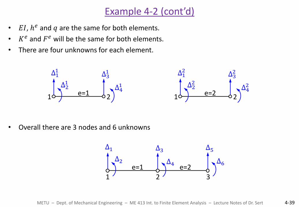
• 𝐸𝐼, ℎ𝑒 and 𝑞 are the same for both elements.

• 𝐾𝑒 and 𝐹𝑒 will be the same for both elements.

• There are four unknowns for each element.

• Overall there are 3 nodes and 6 unknowns

Example 4-2 (cont’d)


2 1 e=1

Δ11

Δ21

Δ31

Δ41

2 1 e=2

Δ12

Δ22

Δ32

Δ42

2 1

e=1

Δ1

Δ2

Δ3

Δ4

3

Δ5

Δ6 e=2

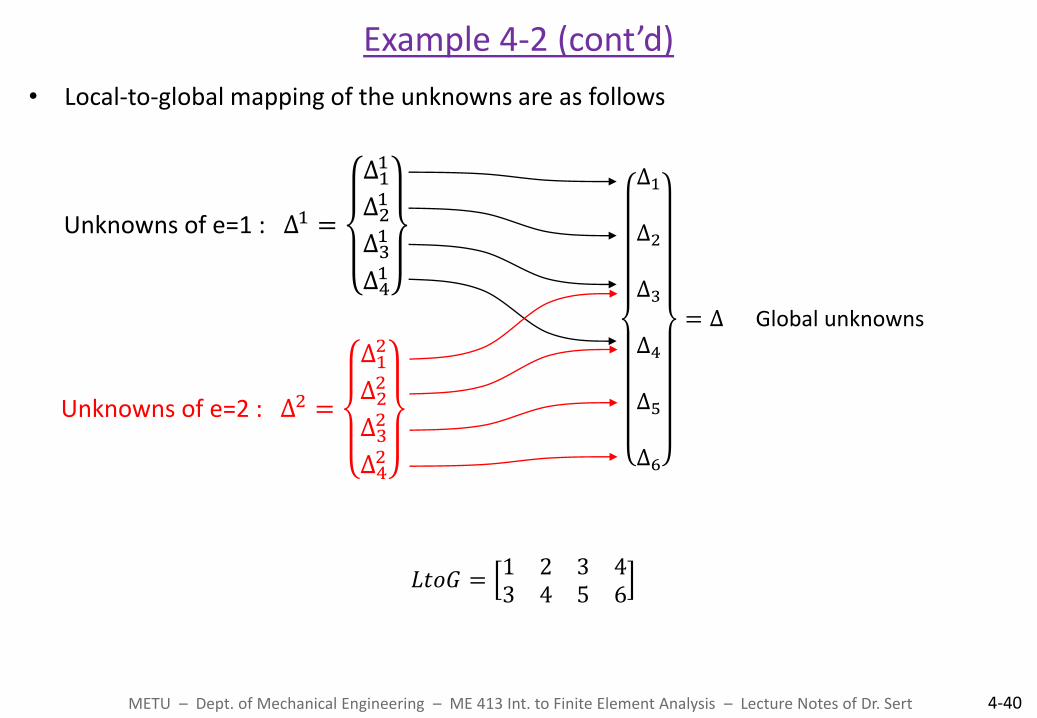
• Local-to-global mapping of the unknowns are as follows



Δ1 Δ2 Δ3 Δ4 Δ5 Δ6

= Δ Global unknowns


Δ11

Δ21

Δ31

Δ41


Δ12

Δ22

Δ32

Δ42

𝐿𝑡𝑜𝐺 =1 2 3 43 4 5 6

• Assembled system is

2𝐸𝐼

(ℎ𝑒)3

6 3ℎ𝑒 −6 3ℎ𝑒 0 03ℎ𝑒 2(ℎ𝑒)2 −3ℎ𝑒 (ℎ𝑒)2 0 0

−6 −3ℎ𝑒 6 + 6 −3ℎ𝑒 + 3ℎ𝑒 −6 3ℎ𝑒

3ℎ𝑒 (ℎ𝑒)2 −3ℎ𝑒 + 3ℎ𝑒 2(ℎ𝑒)2+2(ℎ𝑒)2 −3ℎ𝑒 (ℎ𝑒)2

0 0 −6 −3ℎ𝑒 6 −3ℎ𝑒

0 0 3ℎ𝑒 (ℎ𝑒)2 −3ℎ𝑒 2(ℎ𝑒)2

Δ1Δ2Δ3Δ4Δ5Δ6

=𝑞ℎ𝑒

12

6ℎ𝑒

6 + 6−ℎ𝑒 + ℎ𝑒

6−ℎ𝑒

+

𝑄11

𝑄21

𝑄31 + 𝑄1

2

𝑄41 + 𝑄2

2

𝑄32

𝑄42



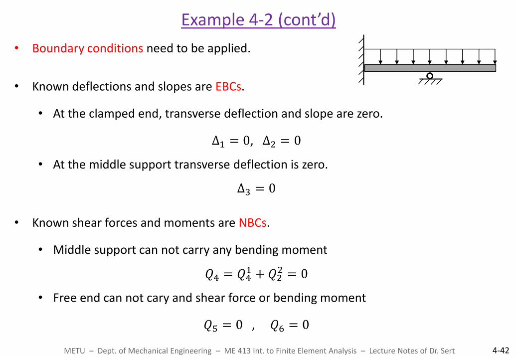
• Boundary conditions need to be applied.

• Known deflections and slopes are EBCs.

• At the clamped end, transverse deflection and slope are zero.

Δ1 = 0, Δ2 = 0

• At the middle support transverse deflection is zero.

Δ3 = 0

• Known shear forces and moments are NBCs.

• Middle support can not carry any bending moment

𝑄4 = 𝑄41 + 𝑄2

2 = 0

• Free end can not cary and shear force or bending moment

𝑄5 = 0 , 𝑄6 = 0



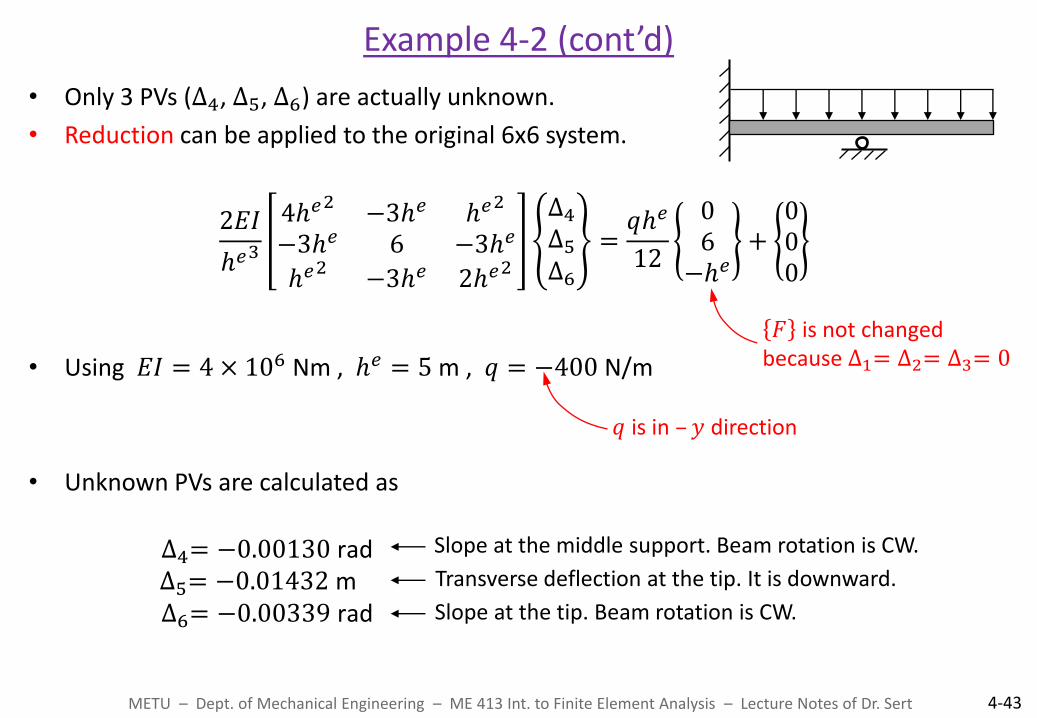
• Only 3 PVs (Δ4, Δ5, Δ6) are actually unknown.

• Reduction can be applied to the original 6x6 system.

2𝐸𝐼

ℎ𝑒3

4ℎ𝑒2−3ℎ𝑒 ℎ𝑒

2

−3ℎ𝑒 6 −3ℎ𝑒

ℎ𝑒2−3ℎ𝑒 2ℎ𝑒

2

Δ4Δ5Δ6

=𝑞ℎ𝑒

12

06−ℎ𝑒+000

• Using 𝐸𝐼 = 4 × 106 Nm , ℎ𝑒 = 5 m , 𝑞 = −400 N/m

• Unknown PVs are calculated as

∆4= −0.00130 rad∆5= −0.01432 m ∆6= −0.00339 rad



𝑞 is in – 𝑦 direction

Slope at the middle support. Beam rotation is CW.

Transverse deflection at the tip. It is downward.

Slope at the tip. Beam rotation is CW.

𝐹 is not changed because ∆1= ∆2= ∆3= 0

• To find the unknown SVs we can use the calculated PVs in the original 6x6 system.

• Unknown SVs can be calculated as

𝑄1 = −250 N 𝑄2 = −1250 Nm𝑄3 = 4250 N



Force applied by the wall at the clamped end.

Moment applied by the wall at the clamped end.

Force acting by the middle support.

4250 N

250 N

1250 Nm

400 N/m

Example 4-3


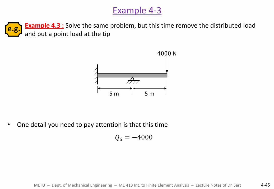
Example 4.3 : Solve the same problem, but this time remove the distributed load and put a point load at the tip

• One detail you need to pay attention is that this time

𝑄5 = −4000

e.g.

4000 N

5 m 5 m

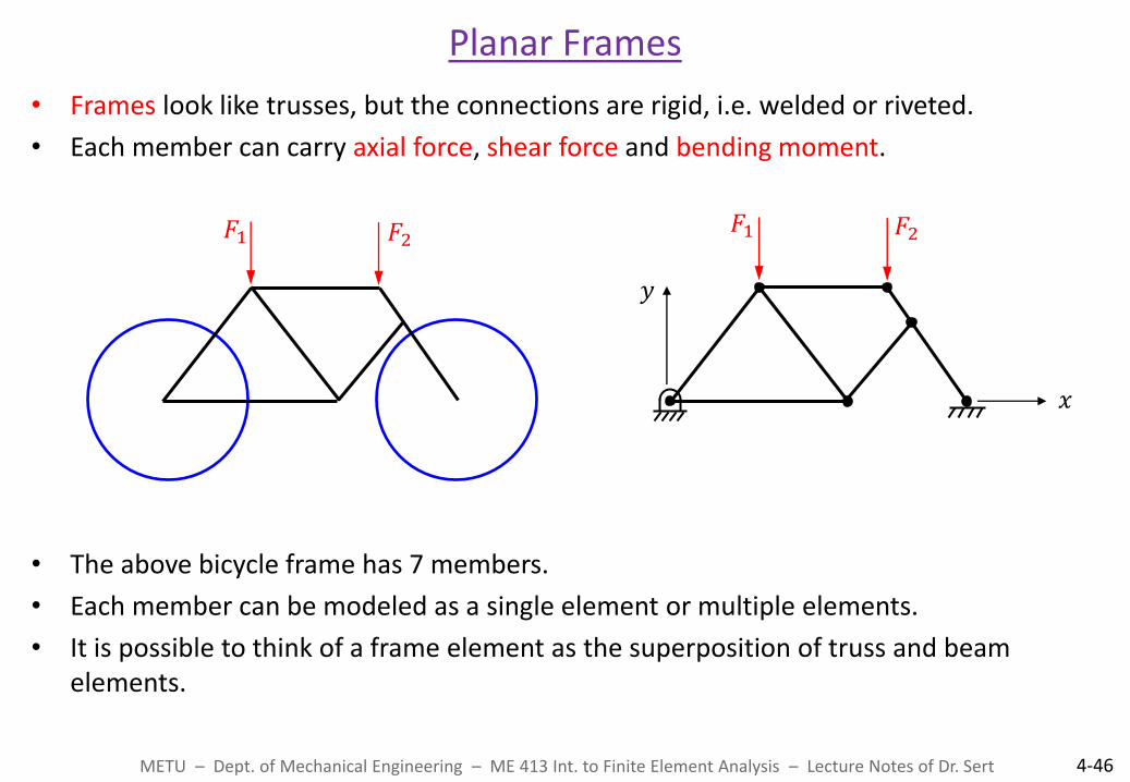
• Frames look like trusses, but the connections are rigid, i.e. welded or riveted.

• Each member can carry axial force, shear force and bending moment.

• The above bicycle frame has 7 members.

• Each member can be modeled as a single element or multiple elements.

• It is possible to think of a frame element as the superposition of truss and beam elements.

Planar Frames


𝐹1 𝐹2

𝑥

𝑦

𝐹1 𝐹2

• Frame elements are based on arbitrarily oriented beam elements.

• Similar to a truss element, it is possible to study the beam element using either the local 𝑥 𝑒, 𝑦 𝑒 coordinates or the global 𝑥, 𝑦 coordinates.

Arbitrarily Oriented Beam Element


𝑥

𝑦

e Δ2𝑒 Δ1𝑒

Δ6𝑒

1

2 Δ3𝑒

Δ5𝑒

Δ4𝑒

e

𝜃𝑒 Δ 2𝑒

Δ 1𝑒

Δ 4𝑒

Δ 3𝑒

𝑥 𝑒

1

2

𝑦 𝑒

Unknowns in local coordinates

Node 1 : Δ 1𝑒 , Δ 2𝑒

Node 2 : Δ 3𝑒 , Δ 3𝑒

Unknowns in global coordinates

Node 1 : Δ1𝑒 , Δ2𝑒 , Δ3𝑒

Node 2 : Δ4𝑒 , Δ5𝑒 , Δ6𝑒

• Relation between local and global unknowns are

Δ 1𝑒 = −sin 𝜃𝑒 Δ1

𝑒 + cos(𝜃𝑒) Δ2𝑒

Δ 2𝑒 = Δ3

𝑒

Δ 3𝑒 = −sin 𝜃𝑒 Δ4

𝑒 + cos(𝜃𝑒) Δ5𝑒

Δ 4𝑒 = Δ6

𝑒

• These relations can be expressed using the following transformation matrix.

Δ 1𝑒

Δ 2𝑒

Δ 3𝑒

Δ 4𝑒

=

−𝛽 𝛼 0 0 0 00 0 1 0 0 00 0 0 −𝛽 𝛼 00 0 0 0 0 1

Δ1𝑒

Δ2𝑒

Δ3𝑒

Δ4𝑒

Δ5𝑒

Δ6𝑒

where 𝛼 = cos(𝜃𝑒) and 𝛽 = sin(𝜃𝑒)

Transformation Matrix of a Beam Element


Transformation matrix of the beam element

• We now have transformation matrices for arbitrarily oriented beam and truss elements.

• Frame elements carry axial force, shear force and bending moment.

• They can be obtained by the superposition of beam and truss elements.

• Frame element has 3 unknowns at each node.

Frame Element


e

𝜃𝑒 Δ 3𝑒

Δ 2𝑒 Δ 6

𝑒

Δ 5𝑒

𝑥 𝑒

1

2

𝑦 𝑒

Δ 1𝑒

Δ 4𝑒

e

Δ3𝑒

Δ2𝑒 Δ6

𝑒

Δ5𝑒

𝑥 1

2

𝑦

Δ1𝑒

Δ4𝑒

Frame element in local coordinates

Frame element in global coordinates

• Elemental system of the frame element in local unknowns is obtained by the proper combination of those of truss and beam elements

𝐾 𝑒 Δ 𝑒 = 𝐹𝑒

𝐸𝐴

ℎ𝑒0 0

−𝐸𝐴

ℎ𝑒0 0

12𝐸𝐼

ℎ𝑒 36𝐸𝐼

ℎ𝑒 20−12𝐸𝐼

ℎ𝑒 36𝐸𝐼

ℎ𝑒 2

4𝐸𝐼

ℎ𝑒0−6𝐸𝐼

ℎ𝑒 22𝐸𝐼

ℎ𝑒

𝐸𝐴

ℎ𝑒0 0

12𝐸𝐼

ℎ𝑒 3−6𝐸𝐼

ℎ𝑒 2

4𝐸𝐼

ℎ𝑒

Δ 1𝑒

Δ 2𝑒

Δ 3𝑒

Δ 4𝑒

Δ 5𝑒

Δ 6𝑒

=

0𝑞ℎ𝑒

2𝑞 ℎ𝑒 2

120𝑞ℎ𝑒

2−𝑞 ℎ𝑒 2

12

Frame Element (cont’d)


These are coming from 𝐾 𝑒 of the truss

element (Slide 4-9)

The rest is coming from 𝐾 𝑒 of the beam

element (Slide 4-37)

𝑞 is the constant distributed transverse load

𝐾 𝑒

{𝐹 𝑒}

Symmetric

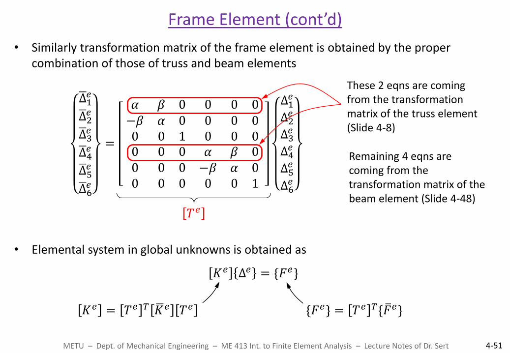
• Similarly transformation matrix of the frame element is obtained by the proper combination of those of truss and beam elements

Δ 1𝑒

Δ 2𝑒

Δ 3𝑒

Δ 4𝑒

Δ 5𝑒

Δ 6𝑒

=

𝛼 𝛽 0 0 0 0−𝛽 𝛼 0 0 0 00 0 1 0 0 00 0 0 𝛼 𝛽 00 0 0 −𝛽 𝛼 00 0 0 0 0 1

Δ1𝑒

Δ2𝑒

Δ3𝑒

Δ4𝑒

Δ5𝑒

Δ6𝑒

• Elemental system in global unknowns is obtained as

𝐾𝑒 Δ𝑒 = {𝐹𝑒}

Frame Element (cont’d)


These 2 eqns are coming from the transformation matrix of the truss element (Slide 4-8)

Remaining 4 eqns are coming from the transformation matrix of the beam element (Slide 4-48)

𝑇𝑒

𝐾𝑒 = 𝑇𝑒 𝑇 𝐾 𝑒 𝑇𝑒 {𝐹𝑒} = 𝑇𝑒 𝑇{𝐹 𝑒}

Example 4-3


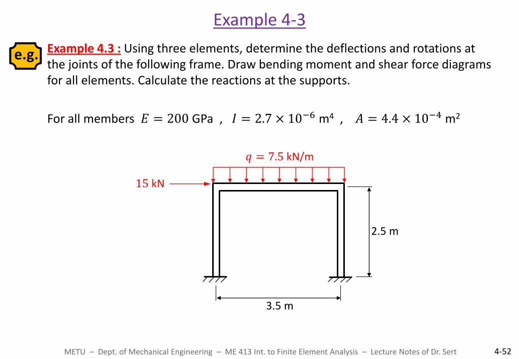
Example 4.3 : Using three elements, determine the deflections and rotations at the joints of the following frame. Draw bending moment and shear force diagrams for all elements. Calculate the reactions at the supports.

For all members 𝐸 = 200 GPa , 𝐼 = 2.7 × 10−6 m4 , 𝐴 = 4.4 × 10−4 m2

e.g.

𝑞 = 7.5 kN/m

3.5 m

2.5 m

15 kN

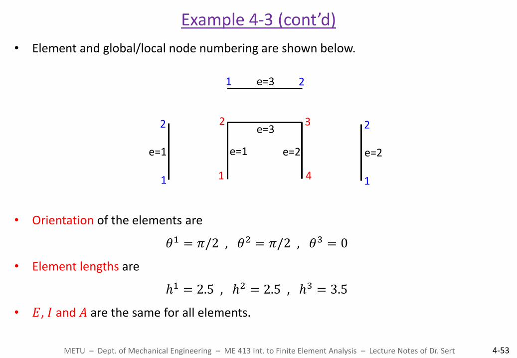
• Element and global/local node numbering are shown below.

• Orientation of the elements are

𝜃1 = 𝜋/2 , 𝜃2 = 𝜋/2 , 𝜃3 = 0

• Element lengths are

ℎ1 = 2.5 , ℎ2 = 2.5 , ℎ3 = 3.5

• 𝐸, 𝐼 and 𝐴 are the same for all elements.



1

2 3

4 1

e=1

e=3

e=2 e=1

2

1

e=2

2

1 2 e=3

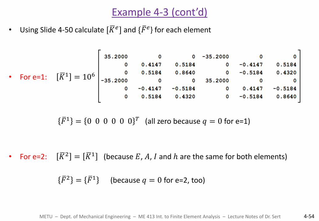
• Using Slide 4-50 calculate [𝐾 𝑒] and {𝐹 𝑒} for each element

• For e=1: 𝐾 1 = 106

𝐹 1 = 0 0 0 0 0 0 𝑇 (all zero because 𝑞 = 0 for e=1)

• For e=2: 𝐾 2 = 𝐾 1 (because 𝐸, 𝐴, 𝐼 and ℎ are the same for both elements)

𝐹 2 = 𝐹 1 (because 𝑞 = 0 for e=2, too)



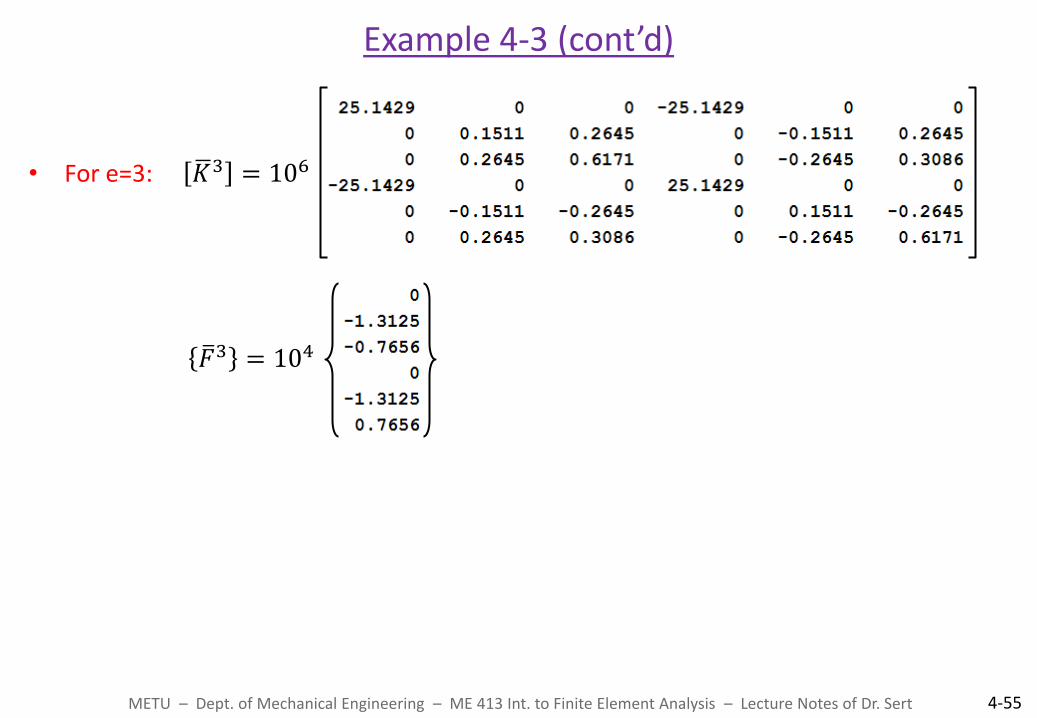
• For e=3: 𝐾 3 = 106

𝐹 3 = 104



• Now the transformation matrices for each element need to be calculated using Slide 4-51.

• For e=1: 𝑇1 =

0 1 0 0 0 0−1 0 0 0 0 00 0 1 0 0 00 0 0 0 1 00 0 0 −1 0 00 0 0 0 0 1

• For e=2: 𝑇2 = 𝑇1 (because 𝜃2 = 𝜃1)

• For e=3: 𝑇3 =

1 0 0 0 0 00 1 0 0 0 00 0 1 0 0 00 0 0 1 0 00 0 0 0 1 00 0 0 0 0 1

(This is the unity matrix because 𝑥 3 = 𝑥)



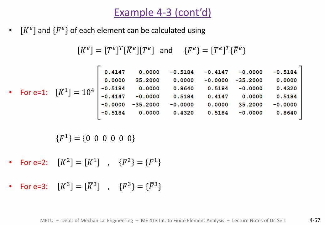
• [𝐾𝑒] and {𝐹𝑒} of each element can be calculated using

𝐾𝑒 = 𝑇𝑒 𝑇 𝐾 𝑒 𝑇𝑒 and {𝐹𝑒} = 𝑇𝑒 𝑇{𝐹 𝑒}

• For e=1: 𝐾1 = 104

𝐹1 = 0 0 0 0 0 0

• For e=2: 𝐾2 = 𝐾1 , 𝐹2 = 𝐹1

• For e=3: 𝐾3 = 𝐾 3 , {𝐹3} = {𝐹 3}



• Now we have three 6x6 elemental systems.

• Let’s assemble them into the 12x12 global system.

• LtoG mapping is as follows

𝐿𝑡𝑜𝐺 =1 2 3 4 5 610 11 12 7 8 94 5 6 7 8 9


1

2 3

4

Δ11 , Δ21 , Δ31

e=1

e=3

e=2 e=1

2

1

e=2

2

1 2 e=3

1

Δ41 , Δ51 , Δ61

Δ12, Δ22 , Δ32

Δ42, Δ52, Δ62

Δ13, Δ23 , Δ33 Δ4

3 , Δ53 , Δ63

Δ1, Δ2, Δ3 Δ10, Δ11, Δ12

Δ4, Δ5, Δ6 Δ7, Δ8, Δ9


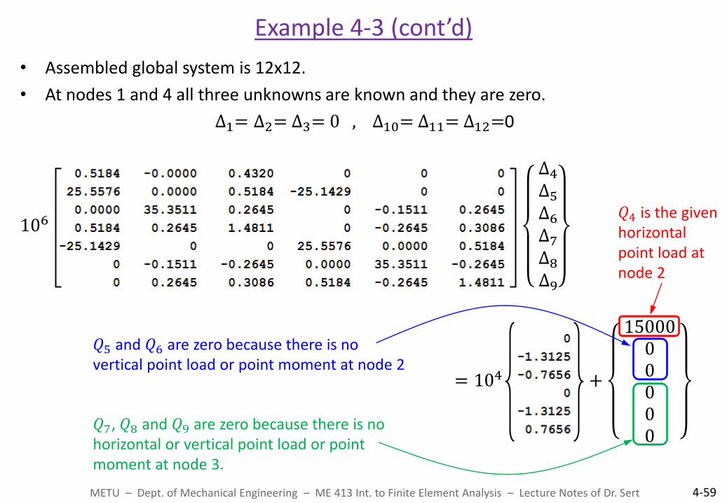
• Assembled global system is 12x12.

• At nodes 1 and 4 all three unknowns are known and they are zero.

∆1= ∆2= ∆3= 0 , ∆10= ∆11= ∆12=0

106

Δ4Δ5Δ6Δ7Δ8Δ9

= 104 +

1500000000


𝑄4 is the given horizontal point load at node 2

𝑄5 and 𝑄6 are zero because there is no vertical point load or point moment at node 2

𝑄7, 𝑄8 and 𝑄9 are zero because there is no horizontal or vertical point load or point moment at node 3.


• Solving for the unknown deflecions we get

Δ4Δ5Δ6Δ7Δ8Δ9

=

• Both nodes 2 and 3 move in +𝑥 and −𝑦 directions. Also they rotate CW.

• Now the forces and moments at the supports (𝑄1, 𝑄2, 𝑄3, 𝑄10, 𝑄11, 𝑄12) can be calculated.

• Also axial stress, shear stress and bending stress over each element can be determined.

• Question : Will the solution improve by using more elements?


Horizontal deflection, vertical deflection and rotation of node 2

Horizontal deflection, vertical deflection and rotation of node 3


Middle East Technical University Department of Mechanical...

Documents

Transcript of Middle East Technical University Department of Mechanical...