Microwave Engineering Course - University of Misan · Microwave Engineering Course 4th Stage...
85
Microwave Engineering Course 4 th Stage Electrical Engineering Department College of Engineering Misan University 2015-2016 Instructor Prof. Dr. Ahmad H. Abood
Transcript of Microwave Engineering Course - University of Misan · Microwave Engineering Course 4th Stage...

Microwave Engineering Course 4th Stage
Electrical Engineering Department
College of Engineering
Misan University
2015-2016
Instructor
Prof. Dr. Ahmad H. Abood

Part VI
Microwave Components

Outline course Resonant cavities
Rectangular cavity resonators
Circular cavity resonators
Q- factor of cavity resonator
Microwave hybrid circuits
The S- parameter theory
Properties of S-parameter
Three port devices
Directional couplers
Outline course

Outline course Circulators and isolators
Hybrid couplers
Outline course

Outline course Resonant cavities
Rectangular cavity resonators
Circular cavity resonators
Q- factor of cavity resonator
Microwave hybrid circuits
The S- parameter theory
Properties of S-parameter
Three point devices
Directional couplers
Outline course
Resonant cavities

Microwave resonators are used in a variety of
applications, including filters, oscillators, frequency meters,
and tuned amplifiers. Because the operation of microwave
resonators is very similar to that of lumped-element
resonators of circuit theory, we will begin by reviewing the
basic characteristics of series and parallel RLC resonant
circuits. We will then discuss various implementations of
resonators at microwave frequencies using distributed
elements such as transmission lines, rectangular and circular
waveguides, and dielectric cavities. We will also discuss the
excitation of resonators using apertures and current sheets.

Outline course Resonant cavities
Rectangular cavity resonators
Circular cavity resonators
Q- factor of cavity resonator
Microwave hybrid circuits
The S- parameter theory
Properties of S-parameter
Three point devices
Directional couplers
Outline course
Rectangular cavity resonators

Microwave resonators can also be constructed from closed sections of
waveguide. Because radiation loss from an open-ended waveguide can be
significant, waveguide resonators are usually short circuited at both ends, thus
forming a closed box, or cavity. Electric and magnetic energy is stored within
the cavity enclosure, and power is dissipated in the metallic walls of the cavity
as well as in the dielectric material that may fill the cavity. Coupling to a
cavity resonator may be by a small aperture, or a small probe or loop. We will
see that there are many possible resonant modes for a cavity resonator,
corresponding to field variations along the three dimensions of the structure.
We will first derive the resonant frequencies for a general TE or TM
resonant mode of a rectangular cavity, and then derive an expression for the unloaded Q of the TE10l mode. A complete treatment of the unloaded Q for
arbitrary TE and TM modes can be made using the same procedure, but is not
included here because of its length and complexity.
Resonant Frequencies
The geometry of a rectangular cavity is shown in Figure 6.6. It consists of a
length, d, of rectangular waveguide shorted at both ends (z = 0, d). We will
find the resonant

frequencies of this cavity under the assumption that the cavity is
lossless, then determine the unloaded Q using the perturbation
method outlined in Section 2.7. Although we could begin with
the Helmholtz wave equation and the method of separation of
variables to solve for the electric and magnetic fields that satisfy
the boundary conditions of the cavity, it is easier to start with the
fields of the TE or TM waveguide modes since these already
satisfy the necessary boundary conditions on the side walls (x =
0, a and y = 0, b) of the cavity. Then it is only necessary to
enforce the boundary conditions that Ex = Ey = 0 on the end walls
at z = 0, d.
The transverse electric fields (Ex , Ey) of the TEmn or TMmn
rectangular waveguide mode can be written as
𝐸 𝑡(𝑥, 𝑦, 𝑧) = 𝑒 (𝑥, 𝑦) 𝐴+𝑒−𝑗𝛽𝑚𝑛𝑧 + 𝐴−𝑒+𝑗𝛽𝑚𝑛𝑧

where 𝑒 (𝑥, 𝑦) is the transverse variation of the mode, and A+, A-
are arbitrary amplitudes of the forward and backward traveling
waves. The propagation constant of the m, nth TE or TM mode is
𝛽𝑚𝑛 = 𝑘2 +𝑚𝜋
𝑎
2
+𝑛𝜋
𝑏
2
where 𝑘 = 𝜔 𝜇𝜀 e and μ and are the permeability and
permittivity of the material filling the cavity. Applying the
condition that 𝐸 𝑡= 0 at z = 0 to (6.36) implies that A+ =−A- (as
we should expect for reflection from a perfectly conducting
wall). Then the condition that 𝐸 𝑡= 0 at z = d leads to the
equation 𝐸 𝑡 = −𝑒 𝑥, 𝑦 𝐴+2𝑗𝑠𝑖𝑛𝛽𝑚𝑛𝑑 = 0
𝛽𝑚𝑛𝑑 = 𝑙𝜋, 𝑙 = 1,2,…
A resonance wave number for the rectangular cavity can be
defined as

𝑘𝑚𝑛𝑙 =𝑚𝜋
𝑎
2
+𝑛𝜋
𝑏
2
+𝑙𝜋
𝑑
2
Then we can refer to the TEmnl or TMmnl resonant mode of the
cavity, where the indices m, n, l indicate the number of variations
in the standing wave pattern in the x, y, z directions, respectively.
The resonant frequency of the TEmnl or TMmnl mode is given by
𝑓𝑚𝑛𝑙 =𝑐𝑘𝑚𝑛𝑙
2𝜋 𝜇𝑟𝜀𝑟=
𝑐
2𝜋 𝜇𝑟𝜀𝑟
𝑚𝜋
𝑎
2
+𝑛𝜋
𝑏
2
+𝑙𝜋
𝑑
2
If b<a<d, the dominant resonant mode (lowest resonant
frequency) will be the TE101 mode, corresponding to the TE10
dominant waveguide mode in a shorted guide of length λg/2, and
is similar to the short-circuited λ/2 transmission line resonator.
The dominant TM resonant mode is the TM110 mode.

The stored electric energy is,
𝑊𝑒 =𝜀
4 𝑬𝑦 ∙ 𝑬𝑦
∗
𝑉
𝑑𝑣 =𝜀
4 𝑬𝑜
2
𝑑
0
𝑠𝑖𝑛𝜋𝑥
𝑎
2
𝑠𝑖𝑛𝜋𝑧
𝑑
2
𝑑𝑥𝑑𝑦𝑑𝑧
𝑏
0
𝑎
0
=𝜀𝑏𝐸𝑜
2
4
1
21 − 𝑐𝑜𝑠
2𝜋𝑥
𝑎𝑑𝑥
𝑎
0
1
21 − 𝑐𝑜𝑠
2𝜋𝑧
𝑑𝑑𝑧
𝑑
0
=𝜀𝑎𝑏𝑑𝐸𝑜
2
16
while the stored magnetic energy is,
𝑊𝑚 =μ
4 (𝑯𝑥 ∙ 𝑯𝑥
∗ + 𝑯𝑧 ∙ 𝑯𝑧∗)
𝑉
𝑑𝑣 =𝜇𝑎𝑏𝑑𝐸𝑜
2
16
1
𝑍𝑇𝐸2 +
𝜋2
𝑘2𝜂2𝑎2 =𝜇𝑎𝑏𝑑𝐸𝑜
2
16𝜂2 = 𝑊𝑒
Showing that We = Wm at resonance. The condition of equal
stored electric and magnetic energies at resonance also applied to
the RLC resonant circuits

Outline course Resonant cavities
Rectangular cavity resonators
Circular cavity resonators
Q- factor of cavity resonator
Microwave hybrid circuits
The S- parameter theory
Properties of S-parameter
Three point devices
Directional couplers
Outline course
Circular cavity resonators

CIRCULAR WAVEGUIDE CAVITY RESONATORS
A cylindrical cavity resonator can be constructed from a section of circular waveguide shorted at both ends, similar to rectangular
cavities. Because the dominant circular waveguide mode is the
TE11 mode, the dominant cylindrical cavity mode is the TE111
mode. We will derive the resonant frequencies for the TEnm and
TMnm circular cavity modes, and an expression for the unloaded
Q of the TEnm mode. Circular cavities are often used for
microwave frequency meters. The cavity is constructed with a
movable top wall to allow mechanical tuning of the resonant
frequency, and the cavity is loosely coupled to a waveguide
through a small aperture. In operation, power will be absorbed by
the cavity as it is tuned to the operating frequency of the system;
this absorption can be monitored with a power meter elsewhere
in the system.

The mechanical tuning dial is usually directly calibrated in
frequency, as in the model shown in Figure 6.7. Because
frequency resolution is determined by the Q of the resonator, the
TE011 mode is often used for frequency meters because its Q is
much higher than the Q of the dominant circular cavity mode.
This is also the reason for a loose coupling to the cavity.
Figure 6.7

Resonant Frequencies
The geometry of a cylindrical cavity is shown in Figure 6.8. As in
the case of the rectangular cavity, the solution is simplified by
beginning with the circular waveguide modes, which already
satisfy the necessary boundary conditions on the wall of the
circular waveguide. From Table 3.5, the transverse electric fields
(Eρ, Eφ) of the TEnm or TMnm circular waveguide mode can be
written as
𝐸 𝑡(𝜌, 𝜙, 𝑧) = 𝑒 (𝜌, 𝜙) 𝐴+𝑒−𝑗𝛽𝑚𝑛𝑧 + 𝐴−𝑒+𝑗𝛽𝑚𝑛𝑧
where 𝑒 (𝜌, 𝜙) represents the transverse variation of the mode,
and A+ and A− are arbitrary amplitudes of the forward and
backward traveling waves. The propagation constant of the TEnm
mode is, from (3.126),
𝛽𝑚𝑛 = 𝑘2 +𝑝′𝑚𝑛
𝑎
2

a
j
z
x 𝑬𝜌 𝑬𝜙
d
a -a
l =1 l =2
d
while the propagation constant of the TMnm mode is, from
(3.139),
𝛽𝑚𝑛 = 𝑘2 +𝑝𝑚𝑛
𝑎
2


Outline course Resonant cavities
Rectangular cavity resonators
Circular cavity resonators
Q- factor of cavity resonator
Microwave hybrid circuits
The S- parameter theory
Properties of S-parameter
Three point devices
Directional couplers
Outline course
Q- factor of cavity resonators

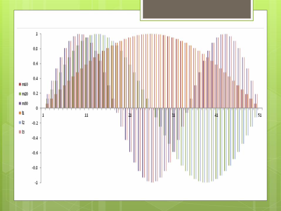
Quality factor: Is the ratio of stored energy to energy dissipated per cycle divided by 2
Stored energy over cavity volume is
where the first integral applies to the time the
energy is stored in the E-field and the second
integral as it oscillates back into the H-field.
dvEW s 2
0
2
edvHW s
20
2
Losses on cavity walls are introduced by
taking into account the finite conductivity of
the walls.
Since, for a perfect conductor, the linear
density of the current J along walls of
structure is 𝑱 = 𝑛 × 𝑯

dss
surf
d HRP
2
2with s = inner surface of conductor
We can write
Rsurf = surface resistance
δ = skin depth
10
fR surf
For Cu, Rsurf = 2.61 10-7 Ω

A. Q- factor of rectangular cavity resonators
The unloaded Q of the cavity with lossy conducting walls but
lossless dielectric can be found as
For small losses we can find the power dissipated in the cavity
walls using the perturbation method of Section 2.7. Thus, the
power lost in the conducting walls is given by(1.131) as
𝑃𝑐 =𝑅𝑠
2 𝐻𝑡
2𝑑𝑠
𝑤𝑎𝑙𝑙
Where 𝑅 = ωμ𝑜/2σ is the surface resistivity of the metallic
walls, and Ht is the tangential magnetic field at the surface of the
walls. Using (6.42b), (6.42c) in (6.44) gives

Unloaded Q of the TE10 Mode
From Table 3.2, (6.36), and the fact that A− = −A+, the total fields
for the TE10 resonant mode can be written as
Letting E0 = −2jA+ and using (6.38) allows these expressions to
be simplified to

𝑷𝒄 =𝑹𝒔
𝟐
𝟐 𝑯𝒙(𝒛 = 𝟎) 𝟐𝒅𝒙𝒅𝒚
𝒂
𝟎
+ 𝟐
𝒃
𝟎
𝑯𝒛(𝒙 = 𝟎) 𝟐𝒅𝒚𝒅𝒛
𝒃
𝟎
+
𝒅
𝟎
𝟐 𝑯𝒙(𝒚 = 𝟎) 𝟐 + 𝑯𝒛(𝒙 = 𝟎) 𝟐 𝒅𝒙𝒅𝒛
𝒂
𝟎
𝒅
𝟎
=𝑹𝒔𝑬𝒐
𝟐𝝀𝟐
𝟖𝜼𝟐
𝒍𝟐𝒂𝒃
𝒅𝟐 +𝒃𝒅
𝒂𝟐 +𝒍𝟐𝒂
𝟐𝒅+
𝒅
𝟐𝒂
where use has been made of the symmetry of the cavity in
doubling the contributions from the walls at x = 0, y = 0, and z =
0 to account for the contributions from the walls at x = a, y = b,
and z = d, respectively. The relations k = 2π/λ and ZTE = kη/β =
2dη/λ were also used in simplifying (6.45). Then, from (6.7), the
unloaded Q of the cavity with lossy conducting walls but lossless
dielectric can be found as


a
b
d
z
y
x
a= 4.755 cm
b= 2.215 cm
d= ?
H band is 6-8 GHz


B. Q- factor of circular cavity resonators
The power loss in the conducting walls is


d
a


Outline course Resonant cavities
Rectangular cavity resonators
Circular cavity resonators
Q- factor of cavity resonator
Microwave hybrid circuits
The S- parameter theory
Properties of S-parameter
Three point devices
Directional couplers
Outline course
Microwave hybrid circuits
Microwave Hybrid Circuits
Microwave circuits consists of several microwave devices
connected in some way to achieve the desired transmission of a
microwave signal. The interconnection of two or more
microwave devices may be regarded as a microwave junction.
Such as waveguide Tees as the E-plane tee, H-plane tee, Magic
tee, hybrid ring tee (rat-race circuit), directional coupler and the
circulator.


Outline course Resonant cavities
Rectangular cavity resonators
Circular cavity resonators
Q- factor of cavity resonator
Microwave hybrid circuits
The S- parameter theory
Properties of S-parameter
Three point devices
Directional couplers
Outline course
The S- parameter theory
Properties of S-parameter

The external behaviour of this
black box can be predicted
without any regard for the contents
of the black box.
This black box could contain
anything:
a resistor,
a transmission line
or an integrated circuit.
S-parameters are a useful method for representing a circuit as a
“black box”

A “black box” or network may have any number of ports.
This diagram shows a simple
network with just 2 ports.
Note :
.pair of linesis a terminal portA

Power, voltage and current
can be considered to be in
the form of waves travelling
in both directions.
For a wave incident on Port 1,
some part of this signal
reflects back out of that port
and some portion of the signal
exits other ports.
S-parameters are measured by sending a single frequency signal
into the network or “black box” and detecting what waves exit
from each port.
For high frequencies, it is
convenient to describe a given
network in terms of waves rather
than voltages or currents. This
permits an easier definition of
reference planes.

.11First lets look at S
S11 refers to the signal
reflected at Port 1 for the
signal incident at Port 1.
Scattering parameter S11
is the ratio of the two
waves b1/a1.
I have seen S-parameters described as S11, S21, etc.
Can you explain?

Now lets look at S21.
S21 refers to the signal
exiting at Port 2 for the
signal incident at Port 1.
Scattering parameter S21
is the ratio of the two
waves b2/a1.
S21? Surely that should be S12??
S21 is correct! S-parameter convention always refers to the
responding port first!
I have seen S-parameters described as S11, S21, etc. Can you
explain?


A linear network can be characterised by a set of simultaneous
equations describing the exiting waves from each port in terms of
incident waves.
S11 = b1 / a1
S12 = b1 / a2
S21 = b2 / a1 or
S22 = b2 / a2
Note again how the subscript follows the parameters in the ratio
(S11=b1/a1, etc...)
I have seen S-parameters described as S11, S21, etc. Can you explain?
𝑺 =
𝑏1
𝑎1
𝑏1
𝑎2
𝑏2
𝑎1
𝑏2
𝑎2
𝑏1
𝑏2=
𝑆11 𝑆12𝑆21 𝑆22
𝑎1
𝑎2
𝑏 = 𝑺𝑎

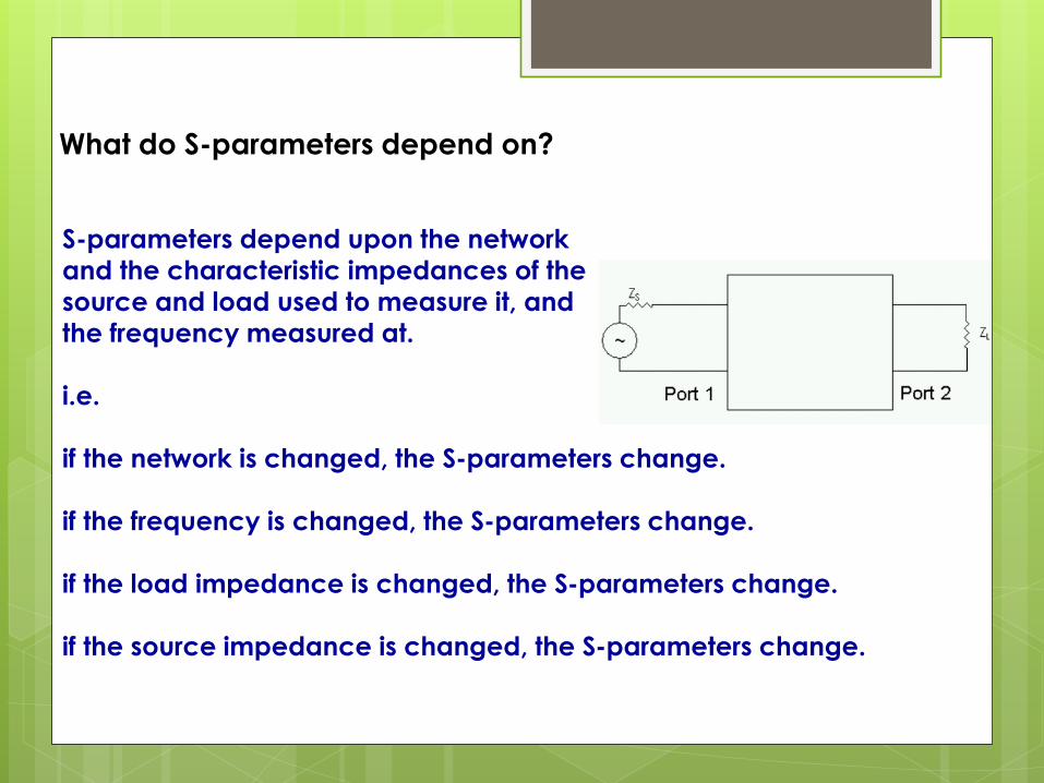
S-parameters depend upon the network
and the characteristic impedances of the
source and load used to measure it, and
the frequency measured at.
i.e.
if the network is changed, the S-parameters change.
if the frequency is changed, the S-parameters change.
if the load impedance is changed, the S-parameters change.
if the source impedance is changed, the S-parameters change.
What do S-parameters depend on?

This is the matrix algebraic representation of 2 port
S-parameters:
Some matrices are symmetrical. A symmetrical
matrix has symmetry about the leading diagonal.
In the case of a symmetrical 2-port network, that
means that S21 = S12 and interchanging the input
and output ports does not change the transmission
properties.
A transmission line is an example of a symmetrical
2-port network.

Parameters along the leading diagonal, S11 &
S22, of the S-matrix are referred to as reflection
coefficients because they refer to the
reflection occurring at one port only.
Off-diagonal S-parameters, S12, S21, are
referred to as transmission coefficients
because they refer to what happens from one
port to another.

𝒂𝟏 𝒂𝟐
𝒂𝟑 𝒂𝟒
𝒃𝟏 𝒃𝟐
𝒃𝟑 𝒃𝟒

Summry
• S-parameters are a powerful way to describe an electrical network
• S-parameters change with frequency / load impedance / source
impedance / network
• S11 is the reflection coefficient
• S21 describes the forward transmission coefficient (responding port 1st!)
• S-parameters have both magnitude and phase information
• Sometimes the gain (or loss) is more important than the phase shift and
the phase information may be ignored
• S-parameters may describe large and complex networks.

Outline course Resonant cavities
Rectangular cavity resonators
Circular cavity resonators
Q- factor of cavity resonator
Microwave hybrid circuits
The S- parameter theory
Properties of S-parameter
Three port devices
Directional couplers
Outline course
Three port devices

• Power division and combining can be achieved with 3-
Port networks.
• For a 3-port network, the S-matrix has 9 elements.
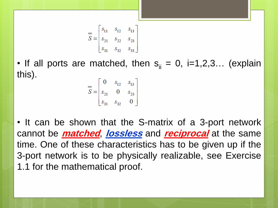
• If all ports are matched, then sii = 0, i=1,2,3… (explain
this).
• It can be shown that the S-matrix of a 3-port network
cannot be matched, lossless and reciprocal at the same
time. One of these characteristics has to be given up if the
3-port network is to be physically realizable, see Exercise
1.1 for the mathematical proof.

• A lossless network results in Unitary S-matrix.
• When the S-matrix is non-reciprocal (sijsji), but the
conditions of port match and lossless apply, the 3-port
network is known as a Circulator.
• Circulator usually has ferrite material at the junction to
cause the non-reciprocity condition.

• A lossy 3-Port network can be reciprocal and matched at
all ports. This type of network is useful as power divider, in
addition it can be made to have isolation between its output
ports (for instance s23 = s32 =0
• A third type of 3-Port network, which is also used as power
divider is reciprocal, lossless and matched at only 2 ports. It
can be shown that its S-matrix is given by:

To fulfill (2) for arbitrary S-parameters, 2 of s12, s13 and s23
must be 0. Substituting this result into (1), it is discovered
that (1) cannot be fulfilled. This leads to a contradiction,
which shows that our assumption of a 3-port network with
matched, reciprocal and lossless conditions is wrong.
…………….(2)
………………(1)

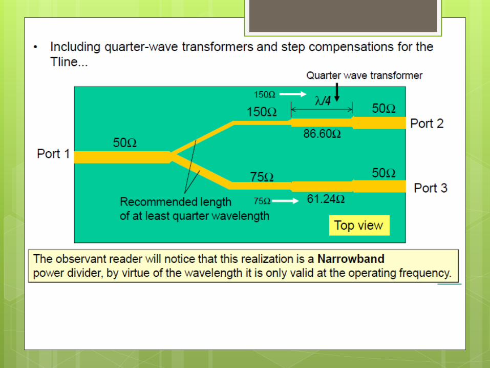
• The T- junction power divider is a simple 3-port network
that can be used for power division or power combining,
and can be implemented on stripline, coaxial cable, and
waveguide technologies.
T- Junction Power Divider
Various Configurations of T- Junction Power Divider

Example 1.2: T- Junction Power Divider Design
• A lossless T-junction power divider has a source
impedance of Zc = 50W. The impedance is matched at the
input. Find the output characteristic impedance so that the
input power is divided in a 2:1 ratio. Compute the reflection
coefficients seen looking into the output ports.
• Implement this power divider using microstrip line on a
printed circuit board.


Outline course Resonant cavities
Rectangular cavity resonators
Circular cavity resonators
Q- factor of cavity resonator
Microwave hybrid circuits
The S- parameter theory
Properties of S-parameter
Three port devices
Directional couplers
Outline course
Directional couplers
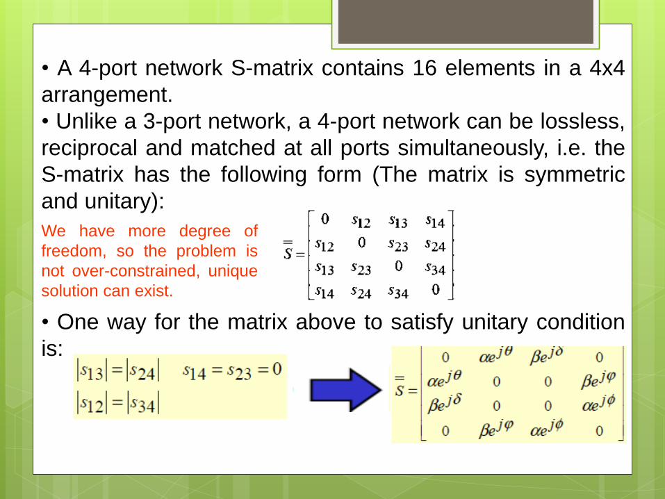
• A 4-port network S-matrix contains 16 elements in a 4x4
arrangement.
• Unlike a 3-port network, a 4-port network can be lossless,
reciprocal and matched at all ports simultaneously, i.e. the
S-matrix has the following form (The matrix is symmetric
and unitary):
We have more degree of
freedom, so the problem is
not over-constrained, unique
solution can exist.
• One way for the matrix above to satisfy unitary condition
is:

• It is customary to fix s12, s13 and s24 as:
• Further application of unitary condition yields:
• Letting n = 0, there are 2 choices that is commonly used
in practice.
• q = f = /2: q = 0, f = :
q +f 2n
or
𝑆12 = 𝑆34 = 𝛼
𝑆13 = 𝛽𝑒𝑗𝛿
𝑆24 = 𝛽𝑒𝑗𝜑


From: paginas.fe.up.pt/~hmiranda/etele/microstrip/

Outline course Circulators and isolators
Hybrid couplers
Outline course
Circulators and isolators

An RF circulator is a three-port
ferromagnetic passive device
used to control the direction of
signal flow in a circuit and is a
very effective, low-cost alternative
to expensive cavity duplexers in
base station and in-building mesh
networks. An RF isolator is a two port
ferromagnetic passive device
which is used to protect other RF
components from excessive
signal reflection. Isolators are
commonplace in laboratory
applications t o separate a device
under test (DUT) from sensitive
signal sources.
Isolator & Circulator Basics
Circulator Isolator

• Both use the unique properties of ferrites in a magnetic
field
• Isolator passes signals in one direction, attenuates in the
other
• Circulator passes input from each port to the next around
the circle, not to any other port

As described earlier, a common application for a circulator is as an inexpensive
duplexer (a device enabling a transmitter and receiver to sharing one antenna).
Figure 2 shows that when the transmitter sends a signal, the output goes
directly to the antenna port and is isolated from the receiver. Good isolation is
key to ensure that a high-power transmitter output signal does not get back to
the receiver front end as is governed by the return loss of the antenna. In this
configuration, all signals from the antenna go straight to the receiver and not
the transmitter because of the circular signal flow (remember the cup of water).
Figure 2: Single Isolator
Clockwise circulation Counterclockwise circulation

Figure 3 illustrates the most common application for an isolator. The
isolator is placed in the measurement path of a test bench between a
signal source and the device under test (DUT) so that any reflections
caused by any mismatches will end up at the termination of the isolator
and not back into the signal source. This example also clearly
illustrates the need to be certain that the termination at the isolated port
is sufficient to handle 100% of the reflected power should the DUT be
disconnected while the signal source is at full power. If the termination
is damaged due to excessive power levels, the reflected signals will be
directed back to the receiver because of the circular signal flow.
Figure 3: Single Isolator

When greater isolation is required, a dual junction isolator
is used as shown in Figure 4. A dual junction isolator is
effectively two isolators in series but contained in a single
package. Typical isolation performance can range from 40
to 50 dB with this type of design.
Figure 4: Dual Junction Isolator

Outline course Circulators and isolators
Hybrid couplers
Outline course
Hybrid coupler

Hybrids
Quadrature Hybrid (90o phase shift)
90o or 180o couplers which split the power equally between direct and
coupled ports are called Hybrids
The basic operation of the branch-line coupler is as follows. With all ports matched,
power entering port 1 is evenly divided between ports 2 and 3, with a 90◦ phase shift
between these outputs. No power is coupled to port 4 (the isolated port). The scattering
matrix has the following form:

The 180o hybrid junction is a four-port network with a 180o phase shift between the
two output ports. It can also be operated so that the outputs are in phase. With reference
to the 180o hybrid symbol shown in Figure 7.41, a signal applied to port 1 will be
evenly split into two in-phase components at ports 2 and 3, and port 4 will be isolated.
If the input is applied to port 4, it will be equally split into two components with a 180o
phase difference at ports 2 and 3, and port 1 will be isolated. When operated as a
combiner, with input signals applied at ports 2 and 3, the sum of the inputs will be
formed at port 1, while the difference will be formed at port 4. Hence, ports 1 and 4 are
referred to as the sum and difference ports, respectively. The scattering matrix for the
ideal 3 dB 180o hybrid thus has the following form:
Quadrature Hybrid (180o phase shift)