Microstructural Finite ElementModeling of Metals

Mikael Nygards

Doctoral Thesis no.53, 2003ISRN KTH/HLF/R- -03/02SE

Department of Solid MechanicsRoyal Institute of Technology

SE-100 44 Stockholm, SWEDEN

Front page: Periodic cell generated by the Voronoi algorithm containing 50 polyhead-rons.

TRITA HLF-0328ISSN 1104-6813ISRN KTH/HLF/R- -03/02- -SE

Akademisk avhandling som med tillstand av Kungliga Tekniska hogskolan i Stockholmframlaggs till offentlig granskning for avlaggande av teknisk doktorsexamen onsda-gen den 16 april 2003 kl 13:15 i kollegiesalen, Valhallavagen 79, Kungliga Tekniskahogskolan i Stockholm.

Preface

When I started as a PhD student in September 1998, I didn’t know much about theDepartment of Solid Mechanics at KTH. Rumors did however say that Professor PeterGudmundson was an excellent advisor. Therefore, I immediately accepted the offer tocome and work for him. I have had no reason to regret that. Now, I can conclude thatPeter is an excellent leader and co-worker that has supported and guided me during thepast years.

This work has been financed by the Swedish Foundation for Strategic Research,SSF, through the Brinell Centre at KTH. The Brinell Centre is a multidisciplinary re-search school where I had the opportunity to meet graduate students from other depart-ments. This has broaden my horizons for research, since I have learnt about researchthat I would not have seen otherwise. At the Brinell centre, the work has been part ofa multidisciplinary project group called Computational Material Science. This projecthas been performed in collaboration with Dilip Chandrasekaran, at the Department ofMaterials Science and Engineering at KTH. We have used the same material to modeldifferent mechanisms, and we have together performed the experiments reported inthe thesis. I really appreciate Dilip’s thorough knowledge of the steels used, and hismicroscopical skills that have been fruitful in analyzing the microstructures.

During two trips to the United States I had the pleasure to travel together withDr Adam Wikstrom. These were great trips where we learned a lot, especially how toget really large rental cars, but also how cooperation can result in papers.

A reliable computer and network is necessary when you do computational work. Iam indebted to Per Berg for suppling that, and also his ability to supply me with thebest and newest computers over the years.

I also want to thank all my other colleagues at the Department of Solid Mechanicsfor making the time at work enjoyable, and especially to all of those participitating inall kinds of sport events that we do.

Lastly, to my beloved wife Karin whom I met, married and built our house withduring the past years. You have given me wonderful life outside work.

Tullinge in February 2003

v

List of appended papers

� Paper A: Micromechanical Modeling of Ferritic/Pearlitic SteelsMikael Nygards and Peter GudmundsonMaterials Science and Engineering A, 325:435-443, 2002.

� Paper B: Three-Dimensional Periodic Voronoi Grain Models and Micromechan-ical FE-Simulations of a Two-Phase SteelMikael Nygards and Peter Gudmundson,Computational Materials Science, 24:513-519, 2002

� Paper C: Anisotropy and texture in Thin Copper Films - an Elasto-Plastic Anal-ysisAdam Wikstrom and Mikael NygardsActa Materialia, 50:857-870, 2002.

� Paper D: Number of grains necessary to homogenize elastic materials with cu-bic symmetryMikael NygardsMechanics of Materials, in press 2003.

� Paper E: Comparison of Surface Displacement Measurements in a Ferritic SteelUsing AFM and Non-Local PlasticityDilip Chandrasekaran and Mikael NygardsReport 329, Department of Solid Mechanics, KTH, Stockholm, 2003Materials Science and Engineering A, in press 2003.

� Paper F: Incorporating Strain Gradients in Micromechanical Modeling of Poly-crystalline AluminumMikael NygardsReport 330, Department of Solid Mechanics, KTH, Stockholm, 2003submitted to Thermec 2003, Madrid, Spain, July 2003.

� Paper G: Numerical Investigation of the Effect of Non-Local Plasticity on Sur-face Roughening in MetalsMikael Nygards and Peter GudmundsonReport 331, Department of Solid Mechanics, KTH, Stockholm, 2003submitted to Mechanics of Materials, 2003.

vii

Abstract

The mechanical properties of metals have been investigated. This has been done bycreating micromechanical models based on the microstructural data available for thematerials of interest. Thus, models containing a grain structure with appropriate con-stitutive equations have been created. Periodic cells on the micrometer scale have beenshown to be sufficient to represent the materials, when macroscopic properties are eval-uated.

Micromechanical modeling by the finite element method can be divided into threedifferent parts: geometry, boundary conditions and constitutive equations. These partshave more or less been illustrated and used in the seven appended papers.

The geometric outlines of the grain structures are represented by the Voronoi algo-rithm. Hence, polyheadrons are used to represent three-dimensional grain structures,while two-dimensional models are represented by polygons. Two different approachesare used. Either, space is divided into grains by application of the Voronoi algorithm.Thus, grain boundaries are represented by planes or lines. Thereafter, the grains aremeshed with an adaptive mesh generator. Alternatively, a mesh is created before theVoronoi algorithm is applied. The grain boundaries will in the latter case be kinky,since the outline of the predefined mesh is followed when grains are formed. The for-mer method results in smaller elements close to grain boundaries. This fact is used tostudy two-phase ferrite-pearlite steels, since pearlite and the small elements have thesame location.

Representative volume elements (RVEs) of the materials are created by consideringa sufficient number of grains, and it is shown how this number depends on anisotropyand loading. To avoid edge effects in the models, the volume elements are made pe-riodic and periodic boundary conditions are utilized to constrain the models. In thepresent implementation of periodic boundary conditions, average stresses and/or aver-age strains are prescribed over the periodic cell.

A non-local crystal plasticity theory that incorporates slip gradients in the harden-ing has been implemented. It is shown that this concept can be used to account for theeffect “smaller is harder”. Furthermore, the effect of non-local plasticity on the defor-mation of a free surface is investigated in detail. It is shown that the surface roughnessdecreases as an effect of strain gradients.

Lastly, all numerical work done here aims to mimic experiments that have beenperformed. This includes microscopic investigations, tensile testing, investigations byatomic force microscopy, but also experimental data from the literature.

ix

Contents

1 Introduction to modeling of materials 11.1 Length scales in modeling of materials . . . . . . . . . . . . . . . . . 11.2 Problem solving strategy . . . . . . . . . . . . . . . . . . . . . . . . 3

2 Material characterization 42.1 Microstructural aspects . . . . . . . . . . . . . . . . . . . . . . . . . 42.2 Grain size and lamellar spacings . . . . . . . . . . . . . . . . . . . . 52.3 Stress-strain relationship . . . . . . . . . . . . . . . . . . . . . . . . 72.4 Hardness . . . . . . . . . . . . . . . . . . . . . . . . . . . . . . . . 10

3 Experimental findings 113.1 The Hall-Petch effect . . . . . . . . . . . . . . . . . . . . . . . . . . 113.2 Local behavior . . . . . . . . . . . . . . . . . . . . . . . . . . . . . 12

3.2.1 Atomic Force Microscopy (AFM) . . . . . . . . . . . . . . . 133.2.2 Speckle methods . . . . . . . . . . . . . . . . . . . . . . . . 133.2.3 Electron backscattered diffraction (EBSD) . . . . . . . . . . . 133.2.4 Future needs . . . . . . . . . . . . . . . . . . . . . . . . . . 13

4 Micromechanical modeling 144.1 Geometrical models . . . . . . . . . . . . . . . . . . . . . . . . . . . 14

4.1.1 Voronoi models . . . . . . . . . . . . . . . . . . . . . . . . . 154.1.2 Micrograph model . . . . . . . . . . . . . . . . . . . . . . . 17

4.2 Representativity . . . . . . . . . . . . . . . . . . . . . . . . . . . . . 174.3 Periodic Boundary Conditions . . . . . . . . . . . . . . . . . . . . . 174.4 Crystal plasticity . . . . . . . . . . . . . . . . . . . . . . . . . . . . 19

4.4.1 Gradient dependent plasticity . . . . . . . . . . . . . . . . . 204.5 Macroscopic properties . . . . . . . . . . . . . . . . . . . . . . . . . 214.6 Local properties . . . . . . . . . . . . . . . . . . . . . . . . . . . . . 214.7 Two-dimensional examples . . . . . . . . . . . . . . . . . . . . . . . 214.8 Computer resources . . . . . . . . . . . . . . . . . . . . . . . . . . . 23

5 Discussion and outlook 27

6 Summary of appended pappers 30

x

Chapter 1

Introduction to modeling ofmaterials

The fields of solid mechanics and materials science are by tradition old and basic areasof knowledge that are mandatory in several engineering programs. Although, those arecutting edge research areas. Great progress is still made within the respective fields.In this thesis, one branch of solid mechanics research (in the borderland to materialsscience) is highlighted by modeling materials via microstructure. If one considers solidmechanics as a discipline where the objective is to create models for material and struc-tural behavior, and materials science as a discipline where mechanisms are studied indetail, then the objective has been to combine these two. Modeling is the primary inter-est, but the models have been formulated by consideration of as much microstructuralinformation as possible. This should be considered as background and motivation forthe research presented here.

The arrangement of crystallites and crystal defects are usually refered to as themicrostructure of materials. This arrangement is of great importance for the mechanicalproperties. A good understanding of the role of the microstructure gives great insightinto the mechanical behavior of materials.

Generally, it is of interest to characterize materials before they are used. Dependingon the use of a material, there are several properties of importance. That can be thematerial’s mechanical, chemical, physical, biological etc. properties. In this thesis,exclusively metals and their mechanical properties are considered. However, in realitya combination of all environmental aspects should be used in the characterization of amaterial.

Modeling of materials may be performed at different length scales, depending onthe area of interest. Even though there are orders of magnitude between the differentscales in modeling of materials, there are still several similarities regarding mechanicalproperties and modeling approaches.

1.1 Length scales in modeling of materials

Depending on how one looks at a material it can differ considerably. With the bare eyeit is difficult to reveal any structure in a piece of steel. A normal person has difficul-ties in determining the mechanical properties by just looking at the material without

1

2 CHAPTER 1. INTRODUCTION TO MODELING OF MATERIALS

instruments. It is usually necessary to polish and etch the surface to reveal the mi-crostructure. At first (almost visible with the bare eye) a mesostructure is visible. Itcan be processing parameters that result in a gradient structure, e.g. different grain sizethrough the specimen. This structure influences the properties quite much, but is alsodifficult to predict since it is a processing effect. Through a microscope it becomesclear that materials have a microstructure. The microstructure of a metal is built byordered blocks (grains), with a distribution of crystallographic orientations (texture).The process where the material is fabricated determines the microstructure. The poly-crystalline structure of grains in metals usually have different size, topology, phase anddispersion. All these parameters affect the mechanical properties of the metal, andmaterials with very different properties can be created by changing these parametersduring processing.

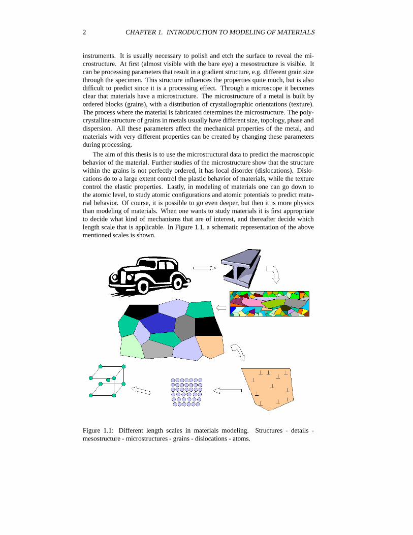
The aim of this thesis is to use the microstructural data to predict the macroscopicbehavior of the material. Further studies of the microstructure show that the structurewithin the grains is not perfectly ordered, it has local disorder (dislocations). Dislo-cations do to a large extent control the plastic behavior of materials, while the texturecontrol the elastic properties. Lastly, in modeling of materials one can go down tothe atomic level, to study atomic configurations and atomic potentials to predict mate-rial behavior. Of course, it is possible to go even deeper, but then it is more physicsthan modeling of materials. When one wants to study materials it is first appropriateto decide what kind of mechanisms that are of interest, and thereafter decide whichlength scale that is applicable. In Figure 1.1, a schematic representation of the abovementioned scales is shown.

Figure 1.1: Different length scales in materials modeling. Structures - details -mesostructure - microstructures - grains - dislocations - atoms.

1.2. PROBLEM SOLVING STRATEGY 3

1.2 Problem solving strategy

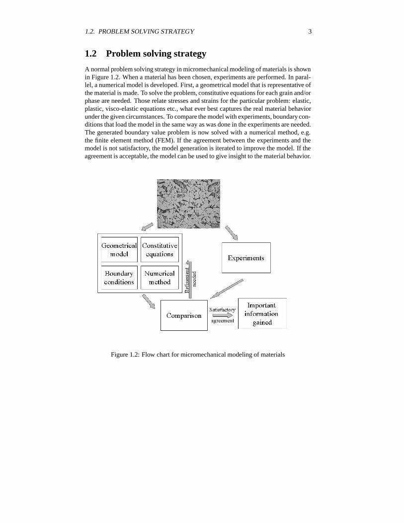
A normal problem solving strategy in micromechanical modeling of materials is shownin Figure 1.2. When a material has been chosen, experiments are performed. In paral-lel, a numerical model is developed. First, a geometrical model that is representative ofthe material is made. To solve the problem, constitutive equations for each grain and/orphase are needed. Those relate stresses and strains for the particular problem: elastic,plastic, visco-elastic equations etc., what ever best captures the real material behaviorunder the given circumstances. To compare the model with experiments, boundary con-ditions that load the model in the same way as was done in the experiments are needed.The generated boundary value problem is now solved with a numerical method, e.g.the finite element method (FEM). If the agreement between the experiments and themodel is not satisfactory, the model generation is iterated to improve the model. If theagreement is acceptable, the model can be used to give insight to the material behavior.

Figure 1.2: Flow chart for micromechanical modeling of materials

Chapter 2

Material characterization

In Paper A, Paper B and Paper E, hot rolled HSLA-steels with varying carbon contentsare chosen as appropriate model materials. The microstructure of these steels usuallyconsists of several phases with different mechanical properties. This makes them suit-able for modeling the effect of different grain structures on the mechanical properties.The general microstructure including specifically the lamellar spacing in the pearliteis investigated. From the mechanical viewpoint, the stress-strain relationship and thehardness of the materials are studied.

2.1 Microstructural aspects

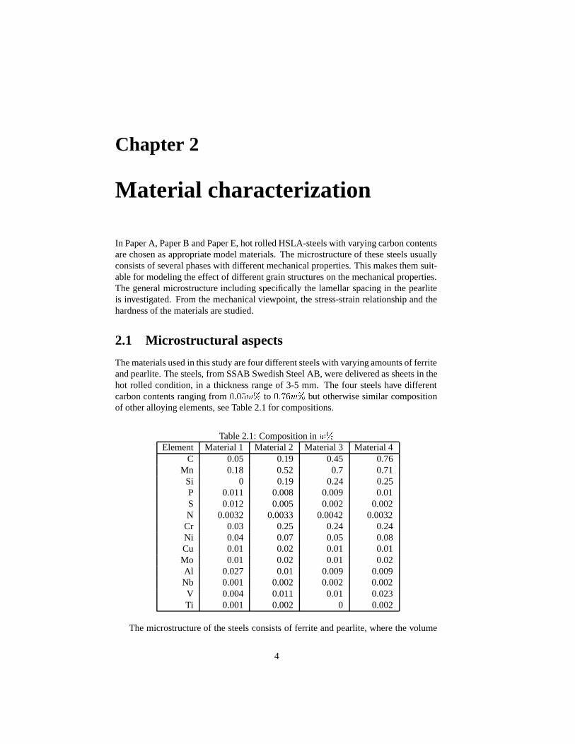
The materials used in this study are four different steels with varying amounts of ferriteand pearlite. The steels, from SSAB Swedish Steel AB, were delivered as sheets in thehot rolled condition, in a thickness range of 3-5 mm. The four steels have differentcarbon contents ranging from ������ to ������ but otherwise similar compositionof other alloying elements, see Table 2.1 for compositions.

Table 2.1: Composition in ��Element Material 1 Material 2 Material 3 Material 4

C 0.05 0.19 0.45 0.76Mn 0.18 0.52 0.7 0.71

Si 0 0.19 0.24 0.25P 0.011 0.008 0.009 0.01S 0.012 0.005 0.002 0.002N 0.0032 0.0033 0.0042 0.0032

Cr 0.03 0.25 0.24 0.24Ni 0.04 0.07 0.05 0.08Cu 0.01 0.02 0.01 0.01Mo 0.01 0.02 0.01 0.02Al 0.027 0.01 0.009 0.009Nb 0.001 0.002 0.002 0.002V 0.004 0.011 0.01 0.023Ti 0.001 0.002 0 0.002

The microstructure of the steels consists of ferrite and pearlite, where the volume

4

2.2. GRAIN SIZE AND LAMELLAR SPACINGS 5

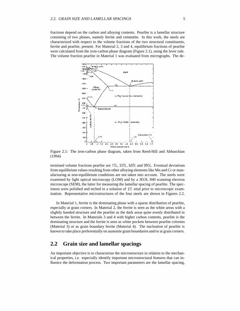
fractions depend on the carbon and alloying contents. Pearlite is a lamellar structureconsisting of two phases, namely ferrite and cementite. In this work, the steels arecharacterized with respect to the volume fractions of the two structural constituents,ferrite and pearlite, present. For Material 2, 3 and 4, equilibrium fractions of pearlitewere calculated from the iron-carbon phase diagram (Figure 2.1), using the lever rule.The volume fraction pearlite in Material 1 was evaluated from micrographs. The de-

Figure 2.1: The iron-carbon phase diagram, taken from Reed-Hill and Abbaschian(1994)

termined volume fractions pearlite are ��, ���, ��� and �. Eventual deviationsfrom equilibrium values resulting from other alloying elements like Mn and Cr or man-ufacturing at non-equilibrium conditions are not taken into account. The steels wereexamined by light optical microscopy (LOM) and by a JEOL 840 scanning electronmicroscope (SEM), the latter for measuring the lamellar spacing of pearlite. The spec-imens were polished and etched in a solution of � nital prior to microscopic exam-ination. Representative microstructures of the four steels are shown in Figures 2.2.

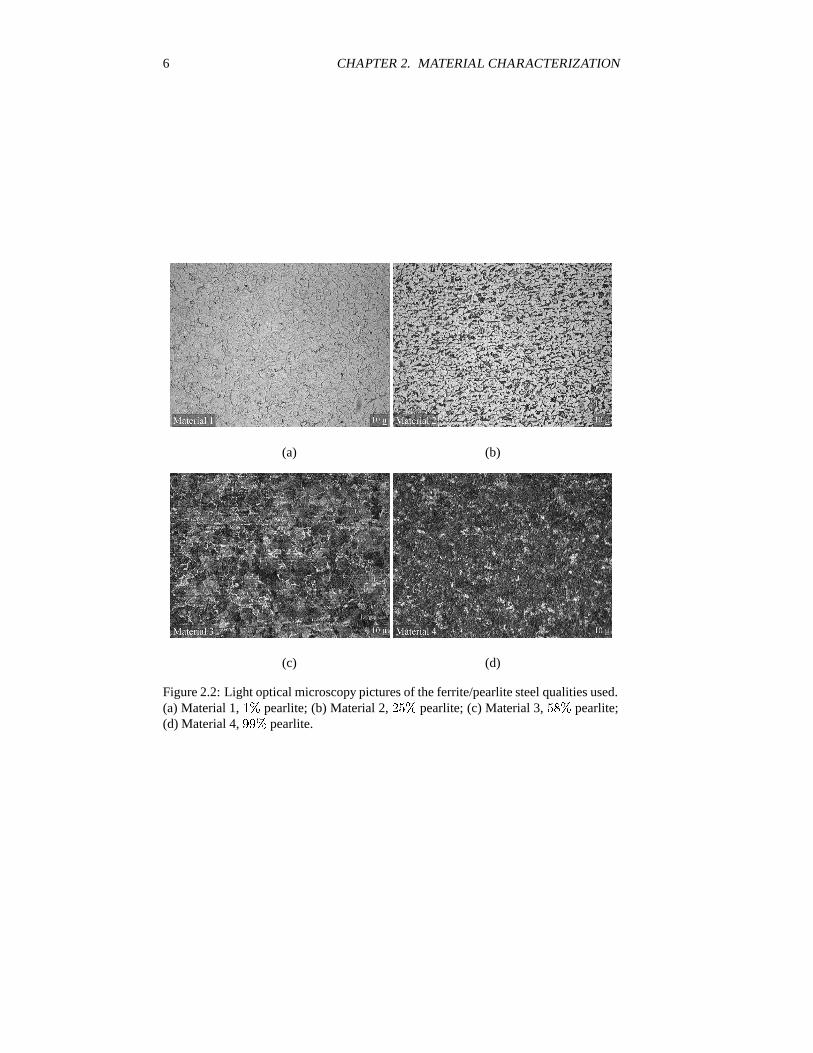
In Material 1, ferrite is the dominating phase with a sparse distribution of pearlite,especially at grain corners. In Material 2, the ferrite is seen as the white areas with aslightly banded structure and the pearlite as the dark areas quite evenly distributed inbetween the ferrite. In Materials 3 and 4 with higher carbon contents, pearlite is thedominating structure and the ferrite is seen as white pockets between pearlite colonies(Material 3) or as grain boundary ferrite (Material 4). The nucleation of pearlite isknown to take place preferentially on austenite grain boundaries and/or at grain corners.

2.2 Grain size and lamellar spacings

An important objective is to characterize the microstructure in relation to the mechan-ical properties, i.e. especially identify important microstructural features that can in-fluence the deformation process. Two important parameters are the lamellar spacing,

6 CHAPTER 2. MATERIAL CHARACTERIZATION

(a) (b)

(c) (d)

Figure 2.2: Light optical microscopy pictures of the ferrite/pearlite steel qualities used.(a) Material 1, �� pearlite; (b) Material 2, ��� pearlite; (c) Material 3, ��� pearlite;(d) Material 4, � pearlite.

2.3. STRESS-STRAIN RELATIONSHIP 7

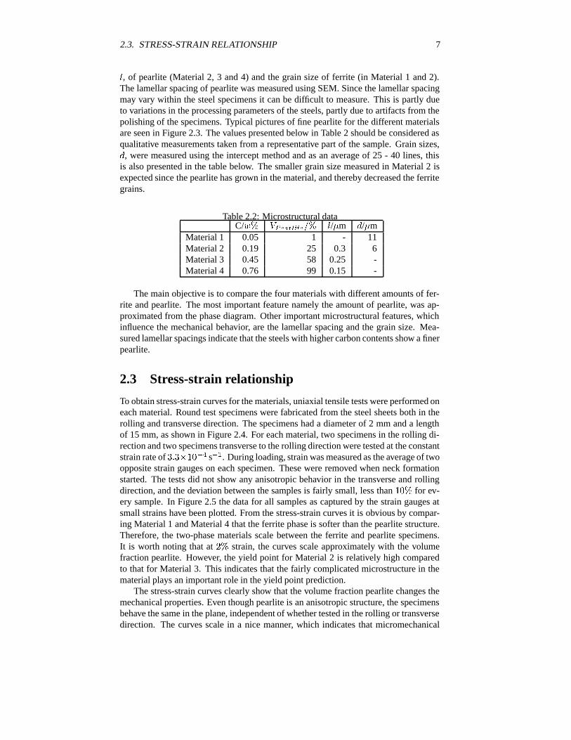
�, of pearlite (Material 2, 3 and 4) and the grain size of ferrite (in Material 1 and 2).The lamellar spacing of pearlite was measured using SEM. Since the lamellar spacingmay vary within the steel specimens it can be difficult to measure. This is partly dueto variations in the processing parameters of the steels, partly due to artifacts from thepolishing of the specimens. Typical pictures of fine pearlite for the different materialsare seen in Figure 2.3. The values presented below in Table 2 should be considered asqualitative measurements taken from a representative part of the sample. Grain sizes,�, were measured using the intercept method and as an average of 25 - 40 lines, thisis also presented in the table below. The smaller grain size measured in Material 2 isexpected since the pearlite has grown in the material, and thereby decreased the ferritegrains.

Table 2.2: Microstructural dataC/�� ����������� �/�m �/�m

Material 1 0.05 1 - 11Material 2 0.19 25 0.3 6Material 3 0.45 58 0.25 -Material 4 0.76 99 0.15 -

The main objective is to compare the four materials with different amounts of fer-rite and pearlite. The most important feature namely the amount of pearlite, was ap-proximated from the phase diagram. Other important microstructural features, whichinfluence the mechanical behavior, are the lamellar spacing and the grain size. Mea-sured lamellar spacings indicate that the steels with higher carbon contents show a finerpearlite.

2.3 Stress-strain relationship

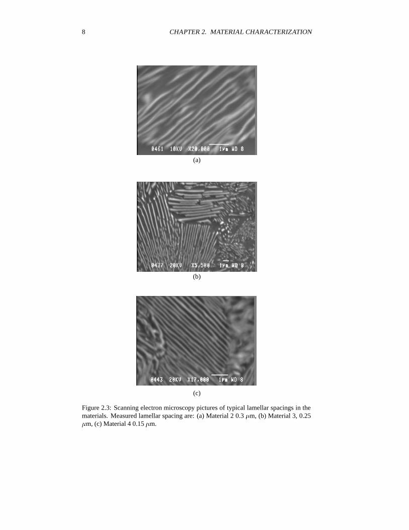
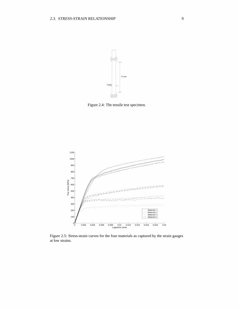
To obtain stress-strain curves for the materials, uniaxial tensile tests were performed oneach material. Round test specimens were fabricated from the steel sheets both in therolling and transverse direction. The specimens had a diameter of 2 mm and a lengthof 15 mm, as shown in Figure 2.4. For each material, two specimens in the rolling di-rection and two specimens transverse to the rolling direction were tested at the constantstrain rate of �������� s��. During loading, strain was measured as the average of twoopposite strain gauges on each specimen. These were removed when neck formationstarted. The tests did not show any anisotropic behavior in the transverse and rollingdirection, and the deviation between the samples is fairly small, less than ��� for ev-ery sample. In Figure 2.5 the data for all samples as captured by the strain gauges atsmall strains have been plotted. From the stress-strain curves it is obvious by compar-ing Material 1 and Material 4 that the ferrite phase is softer than the pearlite structure.Therefore, the two-phase materials scale between the ferrite and pearlite specimens.It is worth noting that at �� strain, the curves scale approximately with the volumefraction pearlite. However, the yield point for Material 2 is relatively high comparedto that for Material 3. This indicates that the fairly complicated microstructure in thematerial plays an important role in the yield point prediction.

The stress-strain curves clearly show that the volume fraction pearlite changes themechanical properties. Even though pearlite is an anisotropic structure, the specimensbehave the same in the plane, independent of whether tested in the rolling or transversedirection. The curves scale in a nice manner, which indicates that micromechanical

8 CHAPTER 2. MATERIAL CHARACTERIZATION

(a)

(b)

(c)

Figure 2.3: Scanning electron microscopy pictures of typical lamellar spacings in thematerials. Measured lamellar spacing are: (a) Material 2 0.3 �m, (b) Material 3, 0.25�m, (c) Material 4 0.15 �m.

2.3. STRESS-STRAIN RELATIONSHIP 9

15 mm

2 mm

Figure 2.4: The tensile test specimen.

0 0.002 0.004 0.006 0.008 0.01 0.012 0.014 0.016 0.018 0.020

100

200

300

400

500

600

700

800

900

1000

1100

Logaritmic strain

Tru

e st

ress

[MP

a]

Material 1Material 2Material 3Material 4

Figure 2.5: Stress-strain curves for the four materials as captured by the strain gaugesat low strains.

10 CHAPTER 2. MATERIAL CHARACTERIZATION

modeling based on microstructural data is possible, in order to predict the deformationbehavior. The deformation seems to follow a parabolic hardening which is as expectedfor these materials. The four steels show a fairly similar hardening behavior, whilethe difference in yield stress is large. This is mainly due to the increasing amountsof pearlite with increasing alloying contents, but also due to an increase in the yieldstrength due to alloying elements by solid solution hardening.

2.4 Hardness

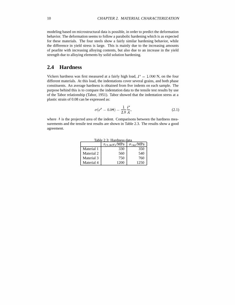
Vickers hardness was first measured at a fairly high load, � � ����� N, on the fourdifferent materials. At this load, the indentations cover several grains, and both phaseconstituents. An average hardness is obtained from five indents on each sample. Thepurpose behind this is to compare the indentation data to the tensile test results by useof the Tabor relationship (Tabor, 1951). Tabor showed that the indentation stress at aplastic strain of 0.08 can be expressed as:

� � ����� ��

���

�

�� (2.1)

where � is the projected area of the indent. Comparisons between the hardness mea-surements and the tensile test results are shown in Table 2.3. The results show a goodagreement.

Table 2.3: Hardness data�����/MPa ���/MPa

Material 1 330 350Material 2 560 540Material 3 750 760Material 4 1200 1250

Chapter 3

Experimental findings

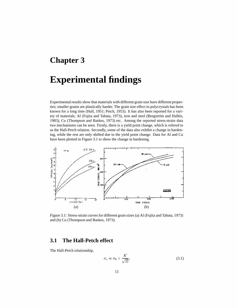
Experimental results show that materials with different grain size have different proper-ties; smaller grains are plastically harder. The grain size effect in polycrystals has beenknown for a long time (Hall, 1951; Petch, 1953). It has also been reported for a vari-ety of materials; Al (Fujita and Tabata, 1973), iron and steel (Bergstrom and Hallen,1983), Cu (Thompson and Baskes, 1973) etc. Among the reported stress-strain datatwo mechanisms can be seen. Firstly, there is a yield point change, which is refered toas the Hall-Petch relation. Secondly, some of the data also exhibit a change in harden-ing, while the rest are only shifted due to the yield point change. Data for Al and Cuhave been plotted in Figure 3.1 to show the change in hardening.

(a) (b)

Figure 3.1: Stress-strain curves for different grain sizes (a) Al (Fujita and Tabata, 1973)and (b) Cu (Thompson and Baskes, 1973).

3.1 The Hall-Petch effect

The Hall-Petch relationship,

� � � � ��� (3.1)

11

12 CHAPTER 3. EXPERIMENTAL FINDINGS

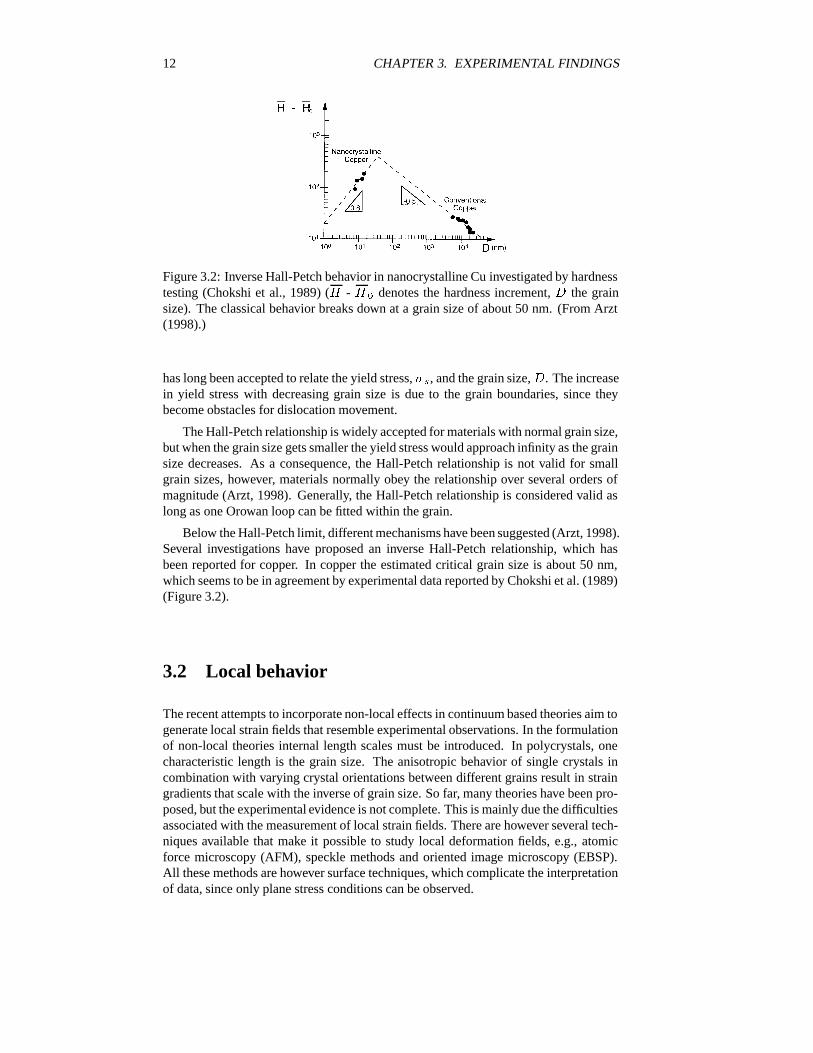
Figure 3.2: Inverse Hall-Petch behavior in nanocrystalline Cu investigated by hardnesstesting (Chokshi et al., 1989) (� - � � denotes the hardness increment, � the grainsize). The classical behavior breaks down at a grain size of about 50 nm. (From Arzt(1998).)

has long been accepted to relate the yield stress, �, and the grain size, �. The increasein yield stress with decreasing grain size is due to the grain boundaries, since theybecome obstacles for dislocation movement.

The Hall-Petch relationship is widely accepted for materials with normal grain size,but when the grain size gets smaller the yield stress would approach infinity as the grainsize decreases. As a consequence, the Hall-Petch relationship is not valid for smallgrain sizes, however, materials normally obey the relationship over several orders ofmagnitude (Arzt, 1998). Generally, the Hall-Petch relationship is considered valid aslong as one Orowan loop can be fitted within the grain.

Below the Hall-Petch limit, different mechanisms have been suggested (Arzt, 1998).Several investigations have proposed an inverse Hall-Petch relationship, which hasbeen reported for copper. In copper the estimated critical grain size is about 50 nm,which seems to be in agreement by experimental data reported by Chokshi et al. (1989)(Figure 3.2).

3.2 Local behavior

The recent attempts to incorporate non-local effects in continuum based theories aim togenerate local strain fields that resemble experimental observations. In the formulationof non-local theories internal length scales must be introduced. In polycrystals, onecharacteristic length is the grain size. The anisotropic behavior of single crystals incombination with varying crystal orientations between different grains result in straingradients that scale with the inverse of grain size. So far, many theories have been pro-posed, but the experimental evidence is not complete. This is mainly due the difficultiesassociated with the measurement of local strain fields. There are however several tech-niques available that make it possible to study local deformation fields, e.g., atomicforce microscopy (AFM), speckle methods and oriented image microscopy (EBSP).All these methods are however surface techniques, which complicate the interpretationof data, since only plane stress conditions can be observed.

3.2. LOCAL BEHAVIOR 13

3.2.1 Atomic Force Microscopy (AFM)

AFM offers the opportunity to study surface topology, and thereby deformations al-ready at initiation of plastic deformation. Essentially, two types of deformations at dif-ferent length scales may be evaluated form the measurements. First, there are discretesteps that form on the surface due to slip bands, which has successfully been studiedby the technique in single crystals (Brinck et al., 1998; Coupeau et al., 1999; Stanfordand Ferry, 2001). Secondly, deformation bands, consisting of many slip bands, canbe studied as they form gradients within grains and closer to boundaries (Tong et al.,1997). The former is of the length of nm, while the latter can be of the length of �m.

3.2.2 Speckle methods

Digital speckle photography is commonly used to map strain fields. A random dottedpattern is applied on the surface, and the displacement field is measured by a compari-son of the pattern before and after deformation. Thereafter, in-plane strain componentsare determined by differention of the displacement fields. The method works well forfairly large specimens, where the camera is placed in front of the specimen, e.g. sheartesting specimens (Petterson, 2002). The method should also work for microstructures,if the camera is mounted on a microscope (microscopic speckle photography). How-ever, it does not seem to have been applied for measurements of local strain fields inpolycrystals.

3.2.3 Electron backscattered diffraction (EBSD)

Plastic deformations generally result in crystal rotations. By the EBSD technique it ispossible to study crystal orientation locally. Thereby, maps of local orientation pertur-bations within grains can be created. The main problem today lies in the interpretationof the results at small deformations. One has to reach deformations of 10-30% toget representative and reproducible results over grain boundaries (Randle et al., 1996;Davies and Randle, 1999, 2000). One possible approach is to use the results and corre-late those to the formation of geometrically necessary dislocations (Sun et al., 1998).

3.2.4 Future needs

All methods mentioned above measure surface activity, although different mechanisms.AFM measures out-of-plane deformation. Speckle methods measure in plane defor-mation, while EBSD measures lattice rotations. Even though different properties aremeasured there should be a relation between the results. The character of deformationis the same. As a material volume deforms it can be elongated, and at the same timerotate and thus also change its out-of-plane position. A very promising and exteremlyinteresting work in this area is done by Chandrasekaran and Nygards (2003). Quany-itative comparisons are made between data from AFM and ESD. Preliminary resultsindicate a close correlation between the two methods. This opens new posibilities fordata evaluation of the two methods.

Chapter 4

Micromechanical modeling

Micromechanical modeling has potential to increase the understanding of material be-havior. A representative volume element (RVE), that has the same average behavioras a larger model, is considered. As discussed in the earlier sections, a polycrystallinematerial consists of grains with different orientations. A micromechanical model of apolycrystalline material should therefore consist of a grain structure. A material canalso have different constituents; a two-phase material has two different materials thatbuild up the grain structure. In micromechanical modeling it is important to catch themost important issues in the model formulation. For a two-phase material, the volumefractions of the two phases may be more important to consider, than the directions ofthe constituents. To create the best model, both issues should however be included.However, at the end of the model generation, it is often necessary to make trade-offsbetween details and computational efficiency. At that point it is important to remem-ber the importance of different effects. Hence, in generating micromechanical modelscertain aspects need to be considered. The following issues should be considered in afinite element model:

� Geometry

� Representativity

� Boundary conditions

� Constitutive equations

4.1 Geometrical models

When accurate stress and strain fields are desired within the RVE, the morphologyshould be as realistic as possible. The microstructure should be represented by agrain structure. Since grain structures are three-dimensional, three-dimensional mod-els should be prefered as was done in Papers B, C, D, E, F and G. However, since thesemodels are computational demanding, two-dimensional approximations can be madein several applications to enlighten certain issues, as was done in Paper A. Below someapproaches to generate geometrical models are outlined.

14

4.1. GEOMETRICAL MODELS 15

4.1.1 Voronoi models

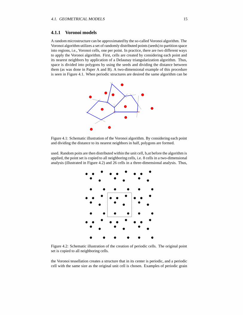
A random microstructure can be approximated by the so-called Voronoi algorithm. TheVoronoi algorithm utilizes a set of randomly distributed points (seeds) to partition spaceinto regions, i.e., Voronoi cells, one per point. In practice, there are two different waysto apply the Voronoi algorithm. First, cells are created by considering each point andits nearest neighbors by application of a Delaunay triangularization algorithm. Thus,space is divided into polygons by using the seeds and dividing the distance betweenthem (as was done in Paper A and B). A two-dimensional example of this procedureis seen in Figure 4.1. When periodic structures are desired the same algorithm can be

Figure 4.1: Schematic illustration of the Voronoi algorithm. By considering each pointand dividing the distance to its nearest neighbors in half, polygons are formed.

used. Random poits are then distributed within the unit cell, b,ut before the algorithm isapplied, the point set is copied to all neighboring cells, i.e. 8 cells in a two-dimensionalanalysis (illustrated in Figure 4.2) and 26 cells in a three-dimensional analysis. Thus,

Figure 4.2: Schematic illustration of the creation of periodic cells. The original pointset is copied to all neighboring cells.

the Voronoi tessellation creates a structure that in its center is periodic, and a periodiccell with the same size as the original unit cell is chosen. Examples of periodic grain

16 CHAPTER 4. MICROMECHANICAL MODELING

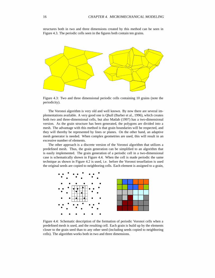
structures both in two and three dimensions created by this method can be seen inFigure 4.3. The periodic cells seen in the figures both contain ten grains.

Figure 4.3: Two and three dimensional periodic cells containing 10 grains (note theperiodicity).

The Voronoi algorithm is very old and well known. By now there are several im-plementations available. A very good one is Qhull (Barber et al., 1996), which createsboth two and three-dimensional cells, but also Matlab (1997) has a two-dimensionalversion. As the grain structure has been generated, the polygons are divided into amesh. The advantage with this method is that grain boundaries will be respected, andthey will thereby be represented by lines or planes. On the other hand, an adaptivemesh generator is needed. When complex geometries are used, this will result in anexcessive number of elements.

The other approach is a discrete version of the Voronoi algorithm that utilizes apredefined mesh. Thus, the grain generation can be simplified to an algorithm thatis easily implemented. The grain generation of a periodic cell in a two-dimensionalcase is schematically shown in Figure 4.4. When the cell is made periodic the sametechnique as shown in Figure 4.2 is used, i.e. before the Voronoi tessellation is usedthe original seeds are copied to neighboring cells. Each element is assigned to a grain,

Figure 4.4: Schematic description of the formation of periodic Voronoi cells when apredefined mesh is used, and the resulting cell. Each grain is build up by the elementscloser to the grain seed than to any other seed (including seeds copied to neighboringcells). The algorithm works both in two and three dimensions.

4.2. REPRESENTATIVITY 17

depending on the closest seed, which is described in Paper D. The fact that the mesh ispredefined makes the latter method very reliable and computational attractive. On theother hand, grain boundaries become very kinky because of the predefined mesh.

4.1.2 Micrograph model

Another approach is to start with an actual photograph of the microstructure, and fromthere create a mesh. For this purpose, NIST has developed a software called Object-Oriented Finite Element Analysis of Real Material Microstructures (OOF) (Carteret al., 2000). The program takes a scanned picture of the microstructure as input, andcreates a mesh. Basically, different phases and/or grains are sorted out because of theircolor.

4.2 Representativity

One of the purposes of micromechanical modeling is to consider only a small part of amaterial. This is possible if the model is a representative volume element. The phraserepresentative volume was introduced by Hill (1963).

In model formulation there is a trade-off between representativity and computa-tional effort. As a model is made larger it becomes more representative, but the mem-ory allocation resources also increases. Thus, the RVE size is mostly determined by thecomputer capacity. Instead, many simulations can be performed, which gives statisti-cal background of the performance of the model. Especially in grain structures, fairlylarge models are needed to achieve representativity. This issue is discussed in detail inPaper D.

Also the material models affect the representativity. In Paper D, elasticity is con-sidered. Plastic deformations normally make materials more isotropic, since a relativesoftening occurs. Evaluation of the number of grains necessary in an elastic analysisshould therefore be an upper limit when plasticity is considered.

4.3 Periodic Boundary Conditions

Boundary conditions corresponding to an average strain � may for a periodic cell beexpressed as

��� � ��� � � �� � �� �� (4.1)

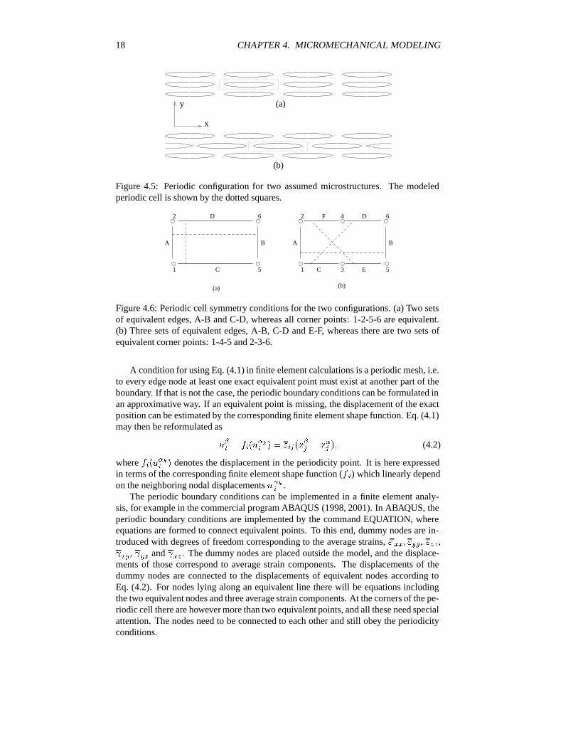
where �� denotes the displacement vector and � the position. In Eq. (4.1), � and �are equivalent boundary points according to the periodicity conditions. In order for aunit cell to be periodic, all outer edges must fulfill a periodicity condition, i.e. everypoint must have at least one equivalent point. As long as periodicity conditions canbe formulated for a given cell, then the same cell can be used to model material withdifferent configurations. In Figure 4.5, two different models of materials are shown.The periodicity is different in the two materials. However the same cell, indicated bythe rectangular box, can be used to model both materials. In this specific case there willbe different numbers of eqivalent edges, as shown in Figure 4.6. The cell (a) has twopairs of equvalent edges, and all corner points are equivalent. Cell (b) on the other handhas three pairs of equivalent edges, and two sets of equvivalent points. More detailsregarding equivalent points and ways to chose the periodic cells can be found in PaperA.

18 CHAPTER 4. MICROMECHANICAL MODELING

y (a)

(b)

x

Figure 4.5: Periodic configuration for two assumed microstructures. The modeledperiodic cell is shown by the dotted squares.

1 5

A

C

A

C

D

B B

D

E

F2 4 6

5 1

2 6

3

(a) (b)

Figure 4.6: Periodic cell symmetry conditions for the two configurations. (a) Two setsof equivalent edges, A-B and C-D, whereas all corner points: 1-2-5-6 are equivalent.(b) Three sets of equivalent edges, A-B, C-D and E-F, whereas there are two sets ofequivalent corner points: 1-4-5 and 2-3-6.

A condition for using Eq. (4.1) in finite element calculations is a periodic mesh, i.e.to every edge node at least one exact equivalent point must exist at another part of theboundary. If that is not the case, the periodic boundary conditions can be formulated inan approximative way. If an equivalent point is missing, the displacement of the exactposition can be estimated by the corresponding finite element shape function. Eq. (4.1)may then be reformulated as

��� � �� ���� � � � �

� � �� �� (4.2)

where �� ���� � denotes the displacement in the periodicity point. It is here expressed

in terms of the corresponding finite element shape function (� �) which linearly dependon the neighboring nodal displacements ���

� .The periodic boundary conditions can be implemented in a finite element analy-

sis, for example in the commercial program ABAQUS (1998, 2001). In ABAQUS, theperiodic boundary conditions are implemented by the command EQUATION, whereequations are formed to connect equivalent points. To this end, dummy nodes are in-troduced with degrees of freedom corresponding to the average strains, ��� ��, ��,���, ��� and ���. The dummy nodes are placed outside the model, and the displace-ments of those correspond to average strain components. The displacements of thedummy nodes are connected to the displacements of equivalent nodes according toEq. (4.2). For nodes lying along an equivalent line there will be equations includingthe two equivalent nodes and three average strain components. At the corners of the pe-riodic cell there are however more than two equivalent points, and all these need specialattention. The nodes need to be connected to each other and still obey the periodicityconditions.

4.4. CRYSTAL PLASTICITY 19

The reaction forces at the dummy nodes may by use of the principle of virtual workbe identified as the corresponding average stresses ��, ��, ��, ���, � ��, ��� timesthe volume of the periodic cell. By this procedure, a complete stress-strain response isevaluated by reading node displacements and node forces of the dummy nodes. Hence,integration is not needed, which simplifies the interpretation of the results considerably.In practice, one loads the model by constraining a combination of average stresses andaverage strains over the periodic cell, while the non-constrained properties are readfrom the nodes.

4.4 Crystal plasticity

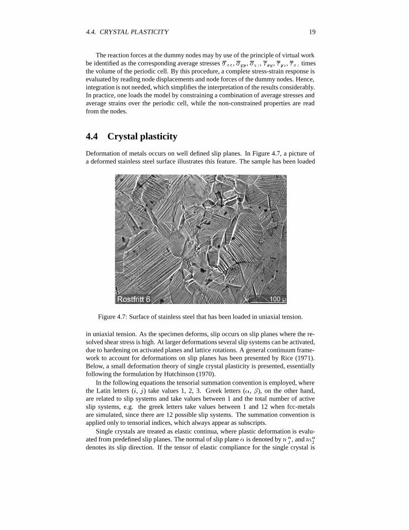
Deformation of metals occurs on well defined slip planes. In Figure 4.7, a picture ofa deformed stainless steel surface illustrates this feature. The sample has been loaded

Figure 4.7: Surface of stainless steel that has been loaded in uniaxial tension.

in uniaxial tension. As the specimen deforms, slip occurs on slip planes where the re-solved shear stress is high. At larger deformations several slip systems can be activated,due to hardening on activated planes and lattice rotations. A general continuum frame-work to account for deformations on slip planes has been presented by Rice (1971).Below, a small deformation theory of single crystal plasticity is presented, essentiallyfollowing the formulation by Hutchinson (1970).

In the following equations the tensorial summation convention is employed, wherethe Latin letters (�, �) take values 1, 2, 3. Greek letters (�, �), on the other hand,are related to slip systems and take values between 1 and the total number of activeslip systems, e.g. the greek letters take values between 1 and 12 when fcc-metalsare simulated, since there are 12 possible slip systems. The summation convention isapplied only to tensorial indices, which always appear as subscripts.

Single crystals are treated as elastic continua, where plastic deformation is evalu-ated from predefined slip planes. The normal of slip plane � is denoted by � �

, and ��

denotes its slip direction. If the tensor of elastic compliance for the single crystal is

20 CHAPTER 4. MICROMECHANICAL MODELING

�� �� and �� denotes the stress tensor, the total strain rate can be expressed as,

�� ��� �� ��� ��

�

��

��� ��� �

� ���

��� �� (4.3)

where �� is slip on slip system �.The resolved shear stress, ��, on each slip plane can be evaluated as,

�� ��

�� �

�� �

� ���

��� �� (no sum on �) (4.4)

On each slip plane there is a critical resolved shear stress, � ���. As deformationprogresses hardening occurs. According to Hill (1965) the rate of change in yieldstresses are assumed to be related to the slip rates of all active slip planes �. Thus, thecritical resolved shear stress on slip plane � changes,

����� ���

��� ��� � (4.5)

where ��� are the instantaneous hardening coefficients, which in general depend on thedeformation history. As the constitutive framework is used to model materials, there isa great variety of functions that can be used to represent different materials. Generally,the coefficients ��� are determined from comparisons to experiments.

In the crystal plasticity implementation used here (Huang, 1991) a visco-plasticformulation is used. Then, the flow rule is formulated as

��� � �����

����

������

����

�������

� (4.6)

where ��� and � are a material constants that need to be defined. If a large power-lawcoefficient � is chosen, � � ��, the formulation is essentially rate independent. In thevisco-plastic formulation all slip planes are potentially active.

4.4.1 Gradient dependent plasticity

A non-local theory has been developed by Acharya and Bassani (1996, 2000) by in-troducing strain gradients in the hardening moduli, ��� . The hardening moduli aremade non-local by incorporating Nye’s (Nye, 1953) tensor � � as a gradient measure,accordingly

��� � ��� ��� �� �� (4.7)

Thus, the hardening moduli depend both on slip and on their graidients through Nye’sdislocation tensor that is used as an incompatibility measure. In crystal plasticity the-ory, Nye’s tensor �� can be expressed as

�� � � ������� � � ��

��

������� �

�� � (4.8)

where � �� is the alternating symbol.There are however outstanding issues on how Nye’s tensor are calculated under

multiple slip (Arsenlis and Parks, 1999). Therefore, another proposal for the incor-poration of plastic strain gradients is given in Paper F. The length of the slip gradientvector is utilized as a parameter that influences the hardening modulus for each slipplane, accordingly,

��� � ��� ��� �������

����� (4.9)

where � is an internal length scale.

4.5. MACROSCOPIC PROPERTIES 21

4.5 Macroscopic properties

When a micromechanical model can be used to homogenize a material behavior themodel is good. To achieve this, macroscopic properties of the model need to be eval-uated. In principle, there are two ways of evaluating macroscopic properties from afinite element model. Firstly, one could do a summation of all stresses and strains inall the elements, and then calculate the averages. Secondly, boundary conditions canbe formulated to simplify the evaluation process, e.g. as described by the periodicboundary condition formulation above. The advantage with the latter approach is thatit simplifies the evaluation considerably. Especially large and complex geometries arepreferably evaluated in this way, compare Paper B.

4.6 Local properties

The purpose of studying the local behavior within an RVE is to gain further insightof the deformation mechanisms. Generally, local properties are more sensitive to dis-cretization errors and geometric simplifications in comparison to macroscopic proper-ties such as average stresses or strains. Therefore, efforts should be made to create asrealistic models as possible before local behavior is studied. Microstructures can e.g.be represented by three-dimensional models as done in Papers B, C, D, F and G.

Especially in Paper C, an attempt is made to evaluate average properties withingrains of different orientations. This is a very enlightening example of how the averagebehavior differs only due to a change of orientation even though the material constantsare the same.

In Papers E and G, local properties are evaluated on a surface. These are goodexamples of how numerical data can be compared to experiments.

4.7 Two-dimensional examples

To demonstrate how different geometrical models behave, three different finite elementbased micromechanical models are presented below. The purpose of all models is togenerate periodic cells representing Material 2 and Material 3, that were character-ized in Chapter 2. These two materials are ferrite/pearlite steels with pearlite fractions0.25 and 0.58 respectively. For this purpose, it is assumed that the ferrite and pearlitehave the same isotropic elastic properties, E=202 GPa and �=0.3, while the plasticproperties differ. The experimental stress-strain curves presented in Paper A for ferrite(Material 1) and pearlite (Material 4) are used as input for the phases’ plastic propertiesin the FE-models. Furthermore, it is assumed that the ferrite phase behaves in the sameway in a two-phase material, as it does as a single phase material. The same assump-tion also goes for the pearlite structure. The intention is thereafter to model the mixedmaterials, based on the volume fraction of the constituent phases.

In Paper A, the generation of two-dimensional periodic cells by the Voronoi algo-rithm for simulation of Material 2 and Material 3 is described in detail. Models are alsogenerated from pictures of microstructures. These micrographs are based on the pic-tures in Figure 2.2b and Figure 2.2c. By use of the program OOF (Carter et al., 2000),meshes with 7240 and 7165 elements for the two materials resulted. The program con-tains a mesh generator and a finite element solver. For present purposes, only the meshgenerator is utilized, since the mesh is exported to ABAQUS (1998), to enable the use

22 CHAPTER 4. MICROMECHANICAL MODELING

of elastic-plastic material models and generalized plane strain elements. As a resultof this approach, unit cells containing 25% and 81% pearlite were created to representMaterial 2 and Material 3.

Some very simple models have also been incorporated in this analysis to investigateif it is worth the effort doing a more sophisticated model. The models have a squareunit cell with a circular inclusion. To model Material 2, the matrix represents theferrite and the circle that fills 25% of the cell represents the pearlite. For Material 3the internal circle represents the ferrite and the matrix the pearlite which in this casefills 58% of the cell. These models are meshed with the same Matlab (1997) routine asthe Voronoi models, which creates a periodic mesh containing 1320 and 1280 elementsrespectively. In addition, inverted circle models were also created. In these, the minorphase represent the matrix, and the major phase the internal circle.

The periodic boundary conditions presented in Eq. (4.1) were utilized for the Voronoimodel, but Eq. (4.2) had to be used on the Micrograph model and circle models, be-cause in these cases the mesh generator did not create a periodic node set.

In addition to the numerical models, also the rule of mixtures for stresses is used tocompare the results. This model can be used for predicting the mechanical behavior oftwo-phase materials. The effective stress is expressed as,

� � �� ��� � ��� (4.10)

where �� is the volume fraction of pearlite, and � and � are the stresses in the ferriteand pearlite at the strain �. This expression has also been used in the analysis for com-parisons with the experimental results and the finite element models. For Material 2,��=0.25 and for Material 3 ��=0.58.

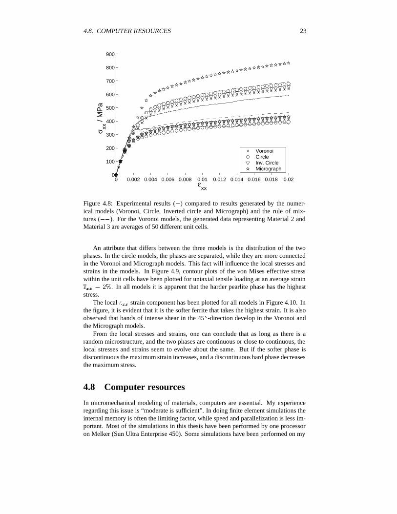
The experimental results, the data generated by the finite element models and byrule of mixture are presented in Figure 4.8. In the figure, the average uniaxial stressin the loading direction �� is plotted versus average strain �� over the representa-tive cell. The Voronoi results represent averages of 50 simulations for each material,where the standard deviation at �� � �� is smaller than 6.4 MPa for Material 2 and14 MPa for Material 3. It is evident that there is a quite good agreement between theexperimental and most simulated data.

For Material 2, the agreement between the experimental data and the Voronoi andcircle model is good at higher strains. The circle model fits quite well to the exper-iments, while the Voronoi model predicts slightly higher stresses. The Micrographmodel and the inverted circle model coincide in the plot, and predict even higherstresses. Compared to the experimental stress at 2% strain, the Voronoi model is 6%and the Micrograph model and inverted circle model are 11% larger.

Unfortunately, none of the models is able to predict the mechanical response ofthe material around the yield point. One can see that the experimental tensile test datahas higher yield stresses than the data generated by the models. This indicates that thefairly complicated microstructure in the two materials plays an important role in theyield point prediction. Possible explanations to the behavior can be that there are eitherLuder band formation, or residual stresses in the phases. None of these effects havebeen incorporated in the models.

For Material 3, all models predict the initial response quite well. The experimen-tal and simulated data capture the same behavior, but as strain increases, the modelspredict higher stresses than the experiments. Compared to the experimental stress at2% strain, the Voronoi model is 7% larger, the inverted circle model is 11% larger, thecircle model is 15% larger and the Micrograph model is as mush as 40% larger.

4.8. COMPUTER RESOURCES 23

0 0.002 0.004 0.006 0.008 0.01 0.012 0.014 0.016 0.018 0.020

100

200

300

400

500

600

700

800

900

εxx

σ xx /

MP

a

Voronoi Circle Inv. CircleMicrograph

Figure 4.8: Experimental results (�) compared to results generated by the numer-ical models (Voronoi, Circle, Inverted circle and Micrograph) and the rule of mix-tures (��). For the Voronoi models, the generated data representing Material 2 andMaterial 3 are averages of 50 different unit cells.

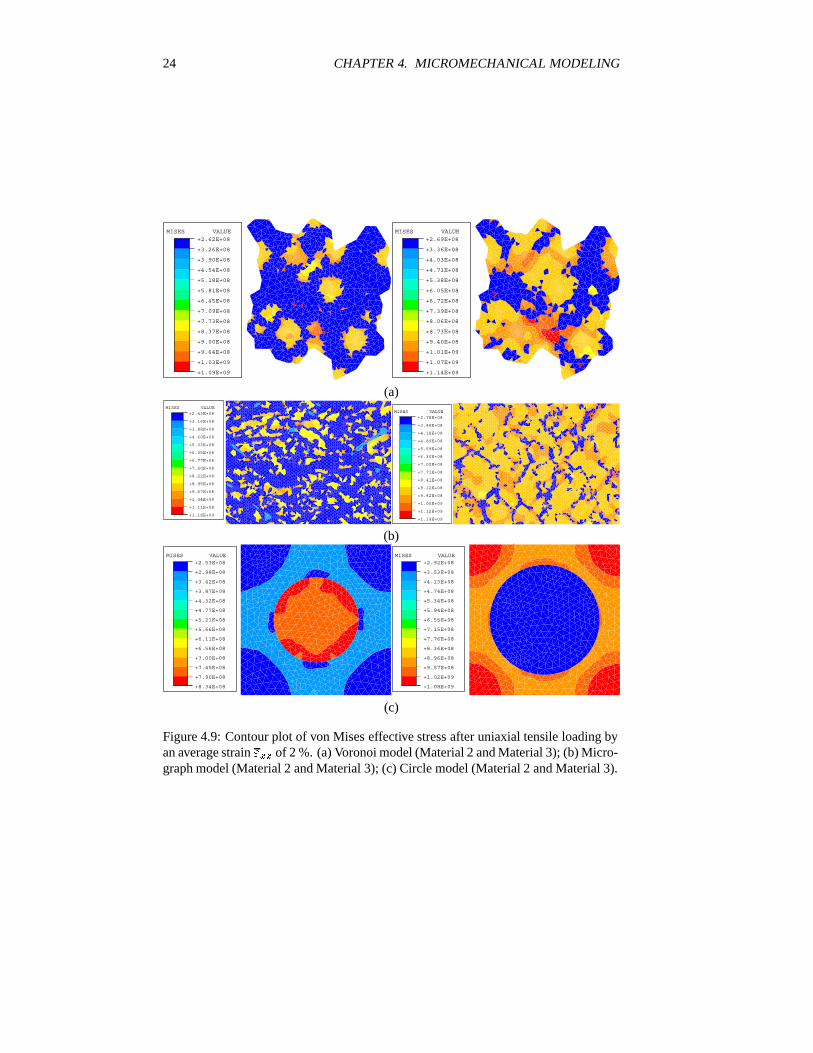
An attribute that differs between the three models is the distribution of the twophases. In the circle models, the phases are separated, while they are more connectedin the Voronoi and Micrograph models. This fact will influence the local stresses andstrains in the models. In Figure 4.9, contour plots of the von Mises effective stresswithin the unit cells have been plotted for uniaxial tensile loading at an average strain�� � ��. In all models it is apparent that the harder pearlite phase has the higheststress.

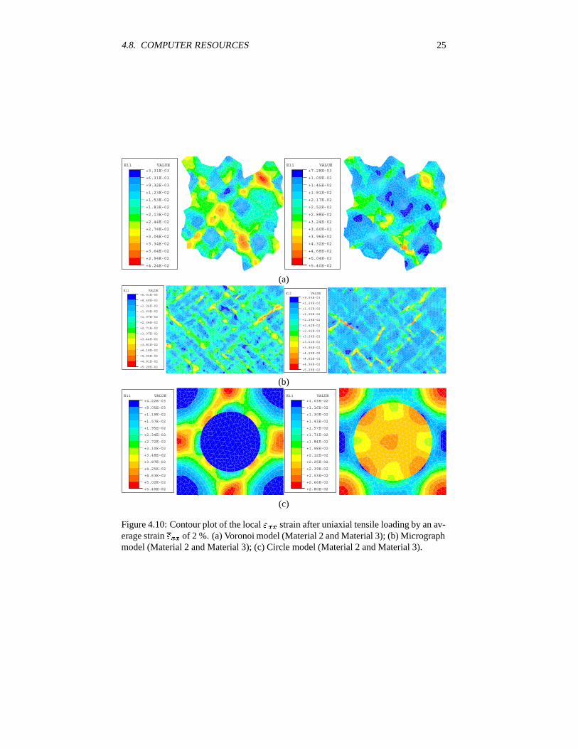
The local �� strain component has been plotted for all models in Figure 4.10. Inthe figure, it is evident that it is the softer ferrite that takes the highest strain. It is alsoobserved that bands of intense shear in the 45�-direction develop in the Voronoi andthe Micrograph models.

From the local stresses and strains, one can conclude that as long as there is arandom microstructure, and the two phases are continuous or close to continuous, thelocal stresses and strains seem to evolve about the same. But if the softer phase isdiscontinuous the maximum strain increases, and a discontinuous hard phase decreasesthe maximum stress.

4.8 Computer resources

In micromechanical modeling of materials, computers are essential. My experienceregarding this issue is “moderate is sufficient”. In doing finite element simulations theinternal memory is often the limiting factor, while speed and parallelization is less im-portant. Most of the simulations in this thesis have been performed by one processoron Melker (Sun Ultra Enterprise 450). Some simulations have been performed on my

24 CHAPTER 4. MICROMECHANICAL MODELING

MISES VALUE+2.62E+08

+3.26E+08

+3.90E+08

+4.54E+08

+5.18E+08

+5.81E+08

+6.45E+08

+7.09E+08

+7.73E+08

+8.37E+08

+9.00E+08

+9.64E+08

+1.03E+09

+1.09E+09

MISES VALUE+2.69E+08

+3.36E+08

+4.03E+08

+4.71E+08

+5.38E+08

+6.05E+08

+6.72E+08

+7.39E+08

+8.06E+08

+8.73E+08

+9.40E+08

+1.01E+09

+1.07E+09

+1.14E+09

(a)MISES VALUE

+2.43E+08

+3.16E+08

+3.88E+08

+4.60E+08

+5.33E+08

+6.05E+08

+6.77E+08

+7.50E+08

+8.22E+08

+8.95E+08

+9.67E+08

+1.04E+09

+1.11E+09

+1.18E+09

MISES VALUE+2.78E+08

+3.48E+08

+4.18E+08

+4.89E+08

+5.59E+08

+6.30E+08

+7.00E+08

+7.71E+08

+8.41E+08

+9.12E+08

+9.82E+08

+1.05E+09

+1.12E+09

+1.19E+09

(b)MISES VALUE

+2.53E+08

+2.98E+08

+3.42E+08

+3.87E+08

+4.32E+08

+4.77E+08

+5.21E+08

+5.66E+08

+6.11E+08

+6.56E+08

+7.00E+08

+7.45E+08

+7.90E+08

+8.34E+08

MISES VALUE+2.92E+08

+3.53E+08

+4.13E+08

+4.74E+08

+5.34E+08

+5.94E+08

+6.55E+08

+7.15E+08

+7.76E+08

+8.36E+08

+8.96E+08

+9.57E+08

+1.02E+09

+1.08E+09

(c)

Figure 4.9: Contour plot of von Mises effective stress after uniaxial tensile loading byan average strain �� of 2 %. (a) Voronoi model (Material 2 and Material 3); (b) Micro-graph model (Material 2 and Material 3); (c) Circle model (Material 2 and Material 3).

4.8. COMPUTER RESOURCES 25

E11 VALUE+3.31E-03

+6.31E-03

+9.32E-03

+1.23E-02

+1.53E-02

+1.83E-02

+2.13E-02

+2.44E-02

+2.74E-02

+3.04E-02

+3.34E-02

+3.64E-02

+3.94E-02

+4.24E-02

E11 VALUE+7.28E-03

+1.09E-02

+1.45E-02

+1.81E-02

+2.17E-02

+2.52E-02

+2.88E-02

+3.24E-02

+3.60E-02

+3.96E-02

+4.32E-02

+4.68E-02

+5.04E-02

+5.40E-02

(a)E11 VALUE

+5.01E-03

+8.68E-03

+1.24E-02

+1.60E-02

+1.97E-02

+2.34E-02

+2.71E-02

+3.07E-02

+3.44E-02

+3.81E-02

+4.18E-02

+4.54E-02

+4.91E-02

+5.28E-02

E11 VALUE+9.55E-03

+1.29E-02

+1.62E-02

+1.95E-02

+2.29E-02

+2.62E-02

+2.96E-02

+3.29E-02

+3.62E-02

+3.96E-02

+4.29E-02

+4.62E-02

+4.96E-02

+5.29E-02

(b)E11 VALUE

+4.22E-03

+8.05E-03

+1.19E-02

+1.57E-02

+1.95E-02

+2.34E-02

+2.72E-02

+3.10E-02

+3.48E-02

+3.87E-02

+4.25E-02

+4.63E-02

+5.02E-02

+5.40E-02

E11 VALUE+1.03E-02

+1.16E-02

+1.30E-02

+1.43E-02

+1.57E-02

+1.71E-02

+1.84E-02

+1.98E-02

+2.12E-02

+2.25E-02

+2.39E-02

+2.53E-02

+2.66E-02

+2.80E-02

(c)

Figure 4.10: Contour plot of the local �� strain after uniaxial tensile loading by an av-erage strain �� of 2 %. (a) Voronoi model (Material 2 and Material 3); (b) Micrographmodel (Material 2 and Material 3); (c) Circle model (Material 2 and Material 3).

26 CHAPTER 4. MICROMECHANICAL MODELING

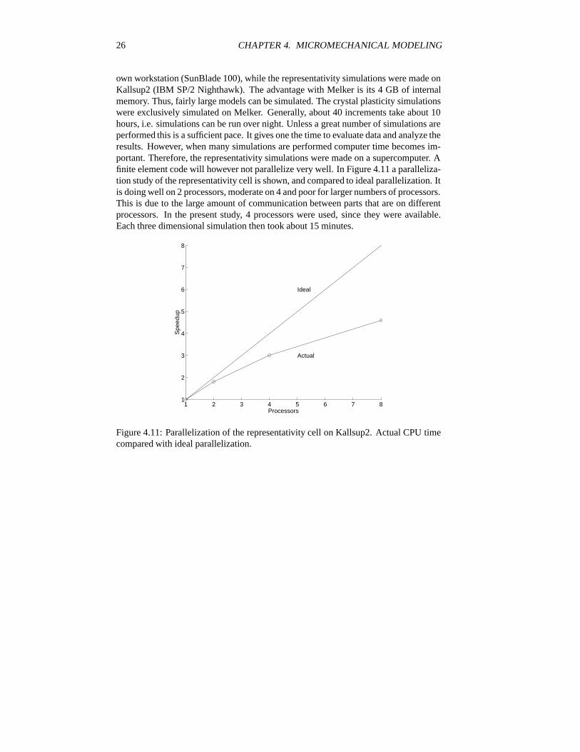
own workstation (SunBlade 100), while the representativity simulations were made onKallsup2 (IBM SP/2 Nighthawk). The advantage with Melker is its 4 GB of internalmemory. Thus, fairly large models can be simulated. The crystal plasticity simulationswere exclusively simulated on Melker. Generally, about 40 increments take about 10hours, i.e. simulations can be run over night. Unless a great number of simulations areperformed this is a sufficient pace. It gives one the time to evaluate data and analyze theresults. However, when many simulations are performed computer time becomes im-portant. Therefore, the representativity simulations were made on a supercomputer. Afinite element code will however not parallelize very well. In Figure 4.11 a paralleliza-tion study of the representativity cell is shown, and compared to ideal parallelization. Itis doing well on 2 processors, moderate on 4 and poor for larger numbers of processors.This is due to the large amount of communication between parts that are on differentprocessors. In the present study, 4 processors were used, since they were available.Each three dimensional simulation then took about 15 minutes.

1 2 3 4 5 6 7 81

2

3

4

5

6

7

8

Processors

Spe

edup

Ideal

Actual

Figure 4.11: Parallelization of the representativity cell on Kallsup2. Actual CPU timecompared with ideal parallelization.

Chapter 5

Discussion and outlook

Over the years the ability to do advanced micromechanical modeling of materials, es-pecially modeling of microstructures, has increased. Since microstructures contain alot of data, models easily become very large and complex. It is therefore easy to realizewhat the increased computer capacity the last 20 years has done. Today one solvesproblems, that 20 years ago were too large, in the matter of seconds. By this revolutionin computer capacity also the complexity of the investigated problems has increased.In the future, even larger problems will most probably be solved. Thus, the ability tomake good research lies in the field of formulating the problems. It is important toconsider the most appropriate mechanisms in defining the problem. The mechanismsshould also be based on a solid physical background before equations are formed.

The ideas and proposed models presented in the thesis have at least one thing incommon. The microstructure of materials is used to gain more information about thematerial. Models have been created to investigate effects of loading, morphology, elas-tic and plastic properties etc. These effects can be difficult to test by experiments. Itcan e.g. be difficult to test a material under biaxial loading, but fairly simple in a nu-merical model. Special care has been made to create geometrical models that haveresemblance to actual microstructures. Geometrical models have been created by theVoronoi algorithm. As the algorithm is used in three dimensions, models with enor-mous complexity can be formed. Even though the models can look complicated tohandle they are straightforward to deal with numerically. This is however due to greatfreeware software that is available at the Internet. As a matter of fact when complicatedproblems are solved, the greatest solutions can be found out there. Even though the ac-tual problem is not available, similar problems often have an existing solution. TheVoronoi algorithm is utilized in several diverse areas, such as: molecular classification,circuit layout, pattern identification and speech coding.

The size of the representative cell in micromechanical modeling is often determinedby the computer capacity. However, details regarding the size determination are oftenfuzzy. One important issue that has not been considered in the thesis is how loadingis prescribed. Periodic boundary conditions and periodic cells have been applied inthe present work. Thus, edge effects are avoided. Another alternative is to prescribestresses and/or strains along the outer boundaries. But, if that is the case boundary layereffects will result. The macroscopic properties will then be altered, and local propertiescan not be studied in the vicinity of the boundaries. Exactly how the macroscopicproperties are affected has not been studied here. One thing is however certain, a largercell than necessary needs to be modeled. In this thesis, a concept that work very well for

27

28 CHAPTER 5. DISCUSSION AND OUTLOOK

modeling of microstructures and that can be improved to have a user friendly interfacehas been developed. The boundary conditions can easily handle any combination ofaverage stress and strain components.

Modeling of materials from microstructure is important since the microstructureeasily is revealed and used to characterize the material. A great challenge lies in theapproach where a grain structure is considered (as done in several papers here). Fromthe revealed microstructure, it is also possible to predict the macroscopic propertieswhen size, constituents, morphology and other relevant paramters are known. On theopposite, it is possible to go down to smaller scales to study certain aspects in moredetail, but then the coupling to macroscopic properties are lost. Therefore, the aim inmicromechanical modeling of materials should be to improve the models, rather thanincreasing the complexity. Detailed studies are however very important backgroundinformation for the creation of appropriate models.

By now we have the ability to do continuum modeling down to the grain level, asshown in this thesis. To create even better micromechanical models the aim shouldbe to improve the constitutive equations. As shown, non-local plasticity theories canpredict a size effect that has been observed in materials science for a very long time.The interest in non-local continuum mechanics theories has however just recently in-creased. This is mainly due to the earlier difficulties in doing advanced models. Nowwhen it becomes possible to implement non-local theories the important task lies indetermining how they should be formulated, and details in the implementions can alsobecome important. The main objective must be to compare numerical work with exper-iments. If the theories are not able to predict classical experimental findings, they willnot last long. It is also very important to get a physical background to proposed models.When a model with a rigid physical basis that predicts experimental work exists, thenwe can start to understand deformation mechanisms within grain structures.

The non-local theory implemented here, where gradients only enter in the harden-ing relation, is fairly straigthforward to implement. This is because an existing FE-codeonly needs little modification. Since only the hardening relations are affected, there isno need to change the equilibrium equations. Therefore, traditional solvers can beused. In other non-local formulations where new equilibrium equations are introduced,the implementation is more complicated. However, interesting work lies ahead thatwill increase the general knowledge about non-local theories, and especailly the use ofthem.

With micromechanical modeling of grain structures it is possible to gain knowledgeabout deformation mechanisms in the micrometer range. If one can predict macro-scopic properties by models like this, then there is an industrial interest in modeling. Ifnew materials can be engineered from results based on simulations, then more adequateexperimental work can be performed from the beginning. Instead of buying/makingmaterials by trial and error more specific demands can be stated if the desired mi-crostructure and properties are known. It is therefore my opinion that the industryshould make greater efforts in continuum modeling of microstructures. There is aninitial effort to create appropriate tools, but thereafter modeling can be very straight-forward. Models are easily changed in the matter of hours to cover new aspects.

In this work the finite element method has been utilized exclusively. The methodis easily applicable to micromechanical problems, since solvers and constitutive equa-tions are implemented in commercial programs. Thus, only the problem formulationneeds to be considered in creating models. However, FEM is very computer intensiveand parallelizations of the codes give only moderate improvements. The question thenarises to what extent FEM can be utilized in modeling of microstructures. As larger

29

models with more grains are considered, more memory is needed. Whether large mod-els will increase the knowledge of materials is questionable, since the amount of dataincreases considerably. Many people will use FEM to model microstructures, but myopinion is that a stage will be reached where no further scientific information is gained.This is mainly due to the character of deformation. Consider a grain structure, wherethe grain boundaries present obstacles for dislocation movements, i.e. contribute tohardening under plastic deformation. Thus, around grain boundaries there is great ac-tivity, while the grain interior is fairly unaffected. If the deformation characteristicsis known within the grains, i.e if dislocation activity could be caught in a continuummodel, then it would be sufficient to model only the grain boundaries, or other obsta-cles. What is needed then is correct constitutive equations. One needs to characterizethe stress and/or strain gradients that appears in materials, and incorporate those in theequations. Large scale problems could then be solved more easily, without an excessiveamount of data from points that play a smaller role in the deformation. But to reachthat stage there are several obstacles that need to be passed (probably through the finiteelement method).

Within the field of micromechanical modeling of metals through grain structuremore work is interesting. I believe that interesting results can be achieved within thesefields:

� Experimental investigation of surfaces (and also of bulk material). Analysis ofthe character of the deformation within grains, and particularly the effect of grainboundaries. Several surface analysis techniques are now becoming availible inmany labs, such as: AFM, EBSD, speckle methods etc.

� Development of phenomenological models to explain the size effect in a contin-uum description.

� Implementation of non-local plasticity theories.

� Development of numerical methods as a complement to the finite element method.

If one leaves the mechanical properties, similar approaches and problems will probablyalso be of interest in the study of magnetic and electrical properties.

Chapter 6

Summary of appended pappers

Paper A:Micromechanical Modeling of Ferritic/Pearlitic Steels

A two-dimensional micromechanical model based on the Voronoi algorithm is pre-sented to model two-phase ferritic/pearlitic steels. Special care is taken to generateperiodic grain structures as well as periodic finite element meshes. The model is eval-uated by generalized plane strain finite element calculations. Periodic representativecells are generated with the desired volume fraction pearlite. Loading by an arbitrarycombination of average stresses or strains is possible by application of periodic bound-ary conditions.

Uniaxial tension tests are performed on pure ferrite and pearlite specimens, as wellas on materials containing 25% and 58% pearlite. Modeling of the two-phase materialswere performed by use of the stress-strain curves of the pure phases, in the descriptionof the plastic properties. Comparisons between generated data and experiments at aloading strain of 2% show good agreement.

Moreover, local stresses and strains are studied within the different unit cells. Inaddition, the model is used to investigate the plastic behavior under biaxial loading. Itis shown that Hill’s yield criterion gives a good fit to the numerical data.

Paper B:Three-Dimensional Periodic Voronoi Grain Models andMicromechanical FE-Simulations of a Two-Phase Steel

A three-dimensional model is proposed for modeling of microstructures. The model isbased on the finite element method with periodic boundary conditions. The Voronoi al-gorithm is used to generate the geometrical model, which has a periodic grain structurethat follows the original boundaries of the Voronoi cells. As an application, the modelis used to simulate two-phase ferrite/pearlite steels. It is shown that periodic cells withonly five grains generate representative stress-strain curves. The model is comparedwith uniaxial tensile tests as well as with a two-dimensional model.

30

31

Paper C:Anisotropy and texture in Thin Copper Films - an Elasto-Plastic Analysis

The role of elastic anisotropy on the stress inhomogeneity and effective behavior ofcolumnar grained textured Cu thin films have been analyzed within a continuum frame-work. The analysis is based on a three-dimensional model of a film/substrate system.The film exhibits a fiber texture with (111), (001) and randomly oriented grains. Mainlytwo load cases have been considered. Biaxial loading of a film deposited on a siliconsubstrate and tensile loading of a film deposited on a polyimide substrate. The stressdistributions in the (111) and (001) grains were generally found to be very differentwhen subjected to biaxial loading and quite similar when subjected to tensile load-ing. When plastic behavior is invoked, a structural hardening effect is observed. Theplastic behavior differs significantly between biaxial and tensile cyclic loading respec-tively. A new orientation dependent hardening law is proposed. This hardening lawcauses the plastic hardening behavior to be orientation dependent and scale with elas-tic anisotropy. The newly proposed hardening law is demonstrated on a film with smallgrain aspect ratio.

Paper D:Number of grains necessary to homogenize elastic mate-rials with cubic symmetry

A numerical model based on the finite element method is presented for modeling ofmicrostructures. The model uses a discrete version of the Voronoi algorithm to partitionthe mesh into grains. The model is utilized to study representativity of grain structures.The number of grains needed in a representative volume element (RVE) is evaluatedfor materials with cubic symmetry and random texture. It is shown that the number ofgrains needed depend on the anisotropy, and a simple expression that relates anisotropyand the number of grains is suggested.

Paper E:Comparison of Surface Displacement Measurements ina Ferritic Steel Using AFM and Non-Local Plasticity

An attempt to experimentally study deformation characteristics around grain bound-aries and analyze the presence of strain gradients is presented. The evolution of sur-face profiles is studied by AFM at relatively small strains. The results indicate thatthis method can be used to draw conclusions about the deformation characteristics,e.g. in large grains the surface profile seems to vary within a grain. This latter effectcan be seen as an indication of the inhomogeneous deformation occurring within largegrains. The results are also compared with FEM calculations using a non-local crystalplasticity theory that incorporates strain gradients in the hardening moduli.

32 CHAPTER 6. SUMMARY OF APPENDED PAPPERS

Paper F:Incorporating Strain Gradients in Micromechanical Mod-eling of Polycrystalline Aluminum

It is a well known fact that polycrystals exhibit a grain size dependence. Traditionalcontinuum models can however not catch this effect. Lately, there has however beenan increased interest in the development of non-local theories, that can account for thesize effect. In this work a non-local crystal plasticity theory is implemented, whereslip gradients enter in the hardening modulus. A new proposal of how the gradientscan be incorporated in the hardening modulus is presented. The non-local theory isused in a three-dimensional finite element model to model Aluminum (Al). A repre-sentative volume element (RVE) containing a random grain structure is used to modelthe material by the finite element method (FEM). Thus, the mesh is partitioned into aperiodic grain structure by a discrete version of the Voronoi algorithm. The model isused to simulate uniaxial tension, by using periodic boundary conditions to constrainthe model. The non-local theory contains an internal length scale � that needs to be setin the model. As the simulations are compared to reported experimental data on Al,the internal length is set. The coupling between the microstructure and the numericalmodel is discussed, and the proposed hardening relation is justified. It is shown that amodel containing 30 grains predict the grain size effect well. But cells containing 15,45 and 60 grains are also investigated. It is shown that the size effect can be predictedby changing the size of the periodic cell, and also by changing the number of grains inthe cell.

Paper G:Numerical Investigation of the Effect of Non-Local Plas-ticity on Surface Roughening in Metals

A non-local crystal plasticity theory that incorporates strain gradients in the hardeningrelation has been implemented. It is proposed that a gradient term enters the hardeningmodulus through a square-root dependence, which introduces an internal length scale.The relation has resemblance to the Hall-Petch relation. Simulations of polycrystallinematerials are performed through a numerical finite element model that partition themesh into grains through a discrete version of the Voronoi algorithm. Numerical simu-lations of a surface and its roughness are performed since it mimics experimental work,and comparisons to experiments are made. The effect of microstructure, the internallength scale, anisotropy and hardening is presented.

Bibliography

ABAQUS (1998). ABAQUS. Hibbitt, Karlsson & Sorensen Inc, Pawtucket, RI, USA,5.8 edition.

ABAQUS (2001). ABAQUS. Hibbitt, Karlsson & Sorensen Inc, Pawtucket, RI, USA,6.2 edition.

Acharya, A. and Bassani, J. (1996). On non-local flow theories that preserve the clas-sical structure of incremental boundary value problems. In Pineau, A. and Zaoui,A., editors, IUTAM Symposium on Micromechanics of Plasticity and Damage ofMultiphase Materials, pages 3–9. Kluwer Academic Publishers.

Acharya, A. and Bassani, J. (2000). Incompatibility and crystal plasticity. J. Mech.Phys. Solids, 48:1565–1595.

Arsenlis, A. and Parks, D. (1999). Crystallographic aspects of geometrically-necessaryand statistically-stored dislocation density. Acta Mater., 47(5):1597–1611.

Arzt, E. (1998). Size effects in materials due to microstructural and dimensional con-straints: a comparative review. Acta Mater., 46(16):5611–5626.

Barber, C., Dobkin, D., and Huhdanpaa, H. (1996). The Quickhull algorithm for con-vex hulls. ACM Trans. on Mathematical Software.

Bergstrom, Y. and Hallen, H. (1983). Hall-petch relationships of iron and steel. MetalScience, 17:341–347.

Brinck, A., Engelke, C., and Neuhauser, H. (1998). Quantitative AFM investigation ofslip line structure in Fe�Al single crystals after deformation at various temperatures.Mater. Sci. Eng. A, 258:37–41.

Carter, W., Langer, S., and Jr., E. F. (2000). The OOF Manual. NIST,http://www.ctcms.nist.gov, 1.0.8.6 edition.

Chandrasekaran, D. and Nygards, M. (2003). A study of the surface deformation be-haviour at grain boundaries in an ultra low-carbon steel. in preparation.

Chokshi, A., Rosen, A., Karch, J., and Gleiter, H. (1989). On the validity of the hall-petch relationship in nanocrystalline materials. Scripta Metall., 23:1679–1683.

Coupeau, C., Bonneville, J., Matterstock, B., Grilhe, J., and Martin, J.-L. (1999). Slipline analysis in Ni�Al by atomic force microscopy. Scripta Mat., 41(9):945–950.

Davies, R. and Randle, V. (1999). Application of crystal orientation mapping to localorientation perturbations. Eur. Phys. J. AP, 7:25–32.

33

34 BIBLIOGRAPHY

Davies, R. and Randle, V. (2000). Orientation perturbations near triple junctions in anon-cell forming aluminium-magnesium alloy. Mater. Sci. Eng. A, 283:251–265.

Fujita, H. and Tabata, T. (1973). The effect of grain size and deformation sub-structureon mechanical properties of polycrystalline aluminum. Acta Metall., 21:355–365.

Hall, E. (1951). The deformation and ageing of mild steel: III discussion of results.Proc. Phys. Soc. B, 64:747–753.

Hill, R. (1963). Elastic properties of reinforced solids: some theoretical principles. J.Mech. Phys. Solids, 11:357–372.

Hill, R. (1965). Generalized constitutive relations for incremental deformation of metalcrystls by multislip. J. Mech. Phys. Solids.

Huang, Y. (1991). A user-subroutine incorporating single crystal plasticity in theabaqus finite element program. Technical report, Division of Applied Sciences, Har-vard University, Cambridge, Massachusetts.

Hutchinson, J. (1970). Elastic-plastic behaviour of polycrystalline metals and compos-ites. Proc. Roy. Soc. Lond. A, 319:247–272.

Matlab (1997). Matlab 5.1. The MathWorks Inc., Natick, Massachusetts 01760, USA,5.1 edition.

Nye, J. (1953). Some geometrically relations in dislocated crystals. Acta Metall.,1:153–162.

Petch, N. (1953). The cleavage strength of polycrystals. J. Iron Steel Inst., 174:25–28.

Petterson, K. (2002). Development of the inclined double notch shear test for de-termination of interlaminar properties of composite laminates. Licentiate Thesis,Department of Solid Mechanics, KTH, Stockholm.

Randle, V., Hansen, N., and Jensen, D. J. (1996). The deformation behaviour of grainboundary regions in polycrystalline aluminium. Phil. Mag. A, 73(2):265–282.

Reed-Hill, R. and Abbaschian, R. (1994). Physical Metallugy Principles. PWS Pub-lishing Company.

Rice, J. (1971). Inelastic constitutive relations for solids: An internal-variable theoryand its application to metal plasticity. J. Mech. Phys. Solids, 19:433–455.

Stanford, N. and Ferry, M. (2001). Observations using atomic force microscopy ofsurface-relief associated with deformation in cube-oriented single crystals. ScriptaMat., 44:941–946.

Sun, S., Adams, B., Shet, C., Saigal, S., and King, W. (1998). Mesoscale investigationof the deformation field of an aluminium bicrystal. Scripta Mat., 39:501–508.

Tabor, D. (1951). Hardness of Metals. Oxford: University Press.

Thompson, A. and Baskes, M. (1973). Influence of grain size on the work hardeningof face-centered cubic polycrystals. Phil. Mag. A, 28:301–308.

Tong, W., Jr., L. H., Weiland, H., and Wieserman, L. (1997). In-situ surface char-acterization of a binary aluminum alloy during tensile deformation. Scripta Mat.,36(11):1339–1344.