MICROSTRUCTURAL DEVELOPMENT AND SULFATE ATTACK MODELING IN

BLENDED CEMENT-BASED MATERIALS

by

Raphaël Tixier

has been approved

December 2000

APPROVED:

, Chair

Supervisory Committee

ACCEPTED:

Department Chair

Dean, Graduate College

iii

ABSTRACT

Blending portland cement with pozzolanic admixtures is an effective way to

improve the strength and durability of concrete. Additional benefits of this approach are

that many pozzolanic materials used for blending today would be otherwise discarded in

landfills. This reuse and recycling approach contributes to the solution of major

environmental problems. To determine the role of a given type of mineral admixture in

concrete, research efforts were carried out in two directions: characterization of the

microstructural and macrostructural properties of candidate materials used for blending

and the effect of microstructural changes on the durability of the material. In order to

achieve the second task, a comprehensive model for the effects of externa l agents on the

integrity of the material is needed. Copper slag was selected as a potential candidate and

important source of mineral admixture for the fabrication of blended cements.

Preliminary experimental results indicated that use of copper slag may result in an

improvement in the resistance to sulfate attack. From the characterization and hydration

viewpoint, this study presents several aspects of the role played by copper slag in the

properties of concrete. Characterization studies describe the chemical, physical and

mineralogical composition of the copper slag using quantitative Xray diffraction,

Differential Thermogravimetry, and Raman Spectroscopy. The potential densification

and increase of strength due to calcium hydroxide was examined by analyzing pastes

made of calcium hydroxide and slag, and pastes made of portland cement and slag. It was

concluded that the increase in strength and durability of cement-based materials with

copper slag is due to a reduction in the capillary porosity, and improved by the minor

iv

pozzolanic properties. A model for the external sulfate attack of concrete was also

developed. The physico-chemical properties of hardened cements are used as inputs to

predict the undesirable expansion of cement-based materials subjected to sulfate attack.

This model is based on a numerical solution of the diffusion-reaction equation. An

innovative concept of moving boundary due to mechanical damage is introduced.

Damage accumulation due to cracking results in a progressive increase of the diffusivity

in the zone comprised between the surface exposed to sulfates and the internal moving

boundary. A well defined boundary separates the uncracked and cracked zones. Cracking

is the consequence of the expansion of ettringite in an initially microcracked brittle

material. Expansion is modelled as the change in volume of calcium aluminates (residual

tricalcium aluminate, calcium aluminate, monosulfate hydrate, and tetracalcium

aluminate hydrate) when they are transformed into ettringite. Cracking causes softening

of the material in the cracked zone, leading to a reduction of the global stiffness of the

body subject to the attack. The outputs of the model are compared to experimental data

from the literature. The diffusion coefficient of the mortar or concrete and the tricalcium

aluminate content of the cement appear to be the most important parameters with respect

to the rate and amplitude of expansion.

v

ACKNOWLEDGMENTS

I would like to express my gratitude to my advisor Professor Barzin Mobasher for

accepting me at Arizona State University, for his guidance during the steps of this

research, for the support he provided to me, and for the numerous discussions we had

about very diverse topics.

I address my sincere thanks to Professors Bill Houston, Emmanuel B. Owusu-

Antwi, and Michael Mamlouk, for participating in the committee and for their

encouragements.

Many persons from the faculty and staff of Arizona State University facilitated

this research: I thank them all. My particular gratitude goes to Mrs. Cynthia H. Polsky

who ran the Raman experiments.

Finally, I would like to thank my family for sharing all the difficulties with me.

vi

TABLE OF CONTENTS

Page

LIST OF TABLES……………………….……………………………………………….ix

LIST OF FIGURES………………………………………………………………………xi

CHAPTER

1 INTRODUCTION………………………………………………………..1

Error! No table of contents entries found.REFERENCES...……………………………………………………………….140

APPENDIX Page

A SOLUTION OF THE FINITE DIFFERENCE SCHEME

FOR THE DIFFUSION-REACTION EQUATION…………..182

B MATLAB PROGRAM FOR NUMERICAL SOLUTION

PRESENTED IN APPENDIX A………………………………189

C SOLUTION OF THE FINITE DIFFERENCE SCHEME

FOR COMPOSITE MATERIAL……………………………...192

D MATLAB PROGRAM FOR NUMERICAL SOLUTION

PRESENTED IN APPENDIX C………………………………202

E NUMERICAL SOLUTION FOR THE DIFFUSION

EQUATION WITH NO REACTION,

WITH A MOVING BOUNDARY……………………………..204

F MATLAB PROGRAM FOR NUMERICAL SOLUTION

vii

PRESENTED IN APPENDIX E………………………………221

G NUMERICAL SOLUTION FOR THE DIFFUSION-REACTION

EQUATION WITH A MOVING BOUNDARY………………227

H MATLAB PROGRAM FOR NUMERICAL SOLUTION

PRESENTED IN APPENDIX G………………………………225

I ESTIMATION OF THE INITIAL CONCENTRATION

IN CALCIUM ALUMINATES IN CONCRETE………………247

J COMPARISON OF DIFFUSION IN AN INFINITELY LONG

CYLINDER OR PRISM………………………………………..250

ix

LIST OF TABLES

Table Page

Error! No table of figures entries found.

xi

LIST OF FIGURES

Figure Page

Error! No table of figures entries found.

CHAPTER 1

INTRODUCTION

The concrete industry is faced to two important challenges, technical and

environmental. On the technical side, although it may be relatively easy to attain the level

of strength required by design criteria, development of criteria for a durability based

design is still an open field. Numerous agents and mechanisms are known to be able to

cause the degradation of the quality of concrete with time. Examples include aggregate-

alkali reaction, carbonation, chloride ingress, delayed ettringite formation, pure water

attack, microbial attack and internal or external sulfate attack. Many of these mechanisms

of deterioration may be related to the microstructure of the material.

Environmental concerns with concrete are mostly due to the production of

cement. Despite notable progress during the last decades, this process is still very energy

consuming, with an energy source which is almost uniquely fossil based. Subsequently,

the cement industry is responsible for releasing in the atmosphere significant quantities of

carbon dioxide. The CO2 release is both from the combustion of the fuel and from the

calcination of the calcareous rocks which are part of the raw materials. Production of

each ton of portland cement releases as much as one ton of CO2.

In the same time, other industries, for example metallurgy, municipal waste

incineration or electricity production, have to cope with the problem of their own by-

products such as slag and fly ash. These waste materials being produced in large amounts

occupy valuable space to be stockpiled or disposed in landfills, and present

2

environmental hazards such as dust contamination or leaching of heavy metals in the

groundwater.

One of the proposed solutions is to recycle certain by-products in concrete, in lieu

of portland cement1. This will reduce the quantity of waste disposal, while decreases the

dependance on the production of cement. Use as a raw material for cement production is

also a possibility. Furthermore, it appears that the introduction of ineral admixtures

improves the microstructure of cement-based materials. This is mainly because the by-

products are chemically reactive, displaying latent hydraulic properties (blast furnace

slags) or pozzolanic properties (fly ash, silica fume). Their physical properties such as

grain shape and particle size distribution, are of great importance in consideration to

aggregate-paste interface characteristics, fresh concrete workability, or packing

efficiency.

To reach the maximum efficiency in using mineral admixtures, it is first necessary

to study their intrinsic physical and chemical properties. This characterization facilitates

the proportioning of the blended cement so that for a given clinker, the desired properties

are attained. Subsequently, the microstructure of the hydration products has to be

examined and compared to that of hydrated plain cement. The microstructural properties

of the paste and the interfacial zone between aggregate and paste determine most of the

macrostructural characteristics, durability to different exposure conditions, mechanical

behavior, porosity, diffusivity and permeability.

3

With proper modeling of the microstructure, and knowledge of the

macrostructural properties, it is possible to model the phenomena involved in durability

problems, such as diffusion and chemical reactions with ingressing ions. The ultimate

stage of this methodology is to predict the life expectancy of the concrete structure, by

determining the effects of aggressive agents on the strength and stiffness of the concrete.

Life cycle cost analysis is then possible.

In a first part, the present study emphasizes the potential use of a particular

mineral admixture, a copper slag produced in Arizona. After reviewing the present

knowledge about copper slag, the mineralogical and chemical properties of this by-

product are established using characterization techniques, and compared to similar

materials. Its potential reactivity is discussed. Then, hydration reaction of portland

cement in presence of copper are being examined following two steps, by studying the

hydration of mixes of lime/copper slag, and then of portland cement/copper slag.

The second part relates to a particular durability topic, the external sulfate attack.

This type of degradation occurs very frequently in the field, and the use of blended

cements has been proven to be effective in preventing it. At first, the consequences of

external sulfate attack are presented and the possible underlying physical and chemical

mechanisms are discussed. After reviewing the models discussed in the literature, a

modelling effort is carried out in several steps involving diffusion, chemical reaction,

damage and existence of a moving boundary. Expansion of concrete with time is the

phenomenon being studied here. The important parameters implicated in the model are

4

detailed. Finally, the model is used to predict several sets of expansion data on mortar

and concrete from the literature. Limitations of both the tests and the model are discussed

in detail. Finally directions to further improve the model are proposed. These

improvements may be achieved through incorporation of other parameters in the model,

and measurements of ill-defined properties.

CHAPTER 2

COPPER SLAG AS PORTLAND CEMENT REPLACEMENT

2.1. Introduction

2.1.1. Metallurgy of copper

The two main modes of extraction of copper from copper ore are the

pyrometallurgical method and the hydrometallurgical method2,3. The pyrometallurgical

method is the only method applicable to ores containing copper- iron-sulfide minerals

(such as chalcopyrite and chalcobornite), which are the most abundant. The waste

material produced by the hydrometallurgical method is not a slag.

Because of the low copper content of the ores (of the order of 0.5%), copper

extraction is achieved in several steps during the smelting operation. Initially a copper

concentrate (25 to 40% Cu) is produced obtained by fine grinding and separation by

flotation. The copper concentrate is smelted at a temperature of 1250°C with the goal of

obtaining an intermediate product, called “matte”, which is enriched in copper by

removing parts of the iron and the sulfur. Smelting slag and sulfur dioxide gas are

generated as by products. Silica is added in the smelting furnace as a “flux” to facilitate

the separation of matte and slag. The matte is mainly made of copper (35 to 70% Cu),

iron and sulfur, the slag of iron and silica.

Smelting can be accomplished by different techniques:

6

q Reverberatory furnace smelting: the concentrate and the flux are heated at

melting temperature but there is only a limited exchange between these

materials and the atmosphere within the furnace.

q Flash furnace smelting: oxygen is injected in the furnace to enhance the

oxidation of iron and sulfur.

q Electric furnace smelting: the heat needed to perform the smelting operation is

brought by passing electricity through the slag. No oxygen is added.

The matte is further “converted” to copper metal (“blister copper”). The

conversion operation oxidizes and removes the remaining iron and sulfur from the matte

by blowing air or oxygen onto the molten matte. More silica flux is added to facilitate the

removal of iron oxides under the form of a converter slag.

In both operations, smelting and converting, iron is oxidized then combined with

silica to form slag, and sulfur is oxidized and is evacuated under the form of sulfur

dioxide.

Blister copper obtained after convertion has to be further refined. This operation

is beyond the scope of the present study.

2.1.2. Processing of copper slags

Since smelting slags contain traces amounts of copper (from 0.5 to 2%), it may or

may be not economical to try to recover this metal by settling the molten slag or flotation

7

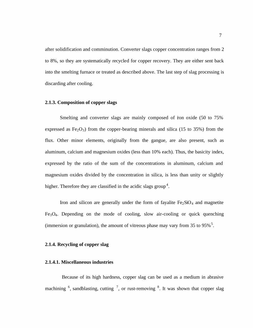
after solidification and comminution. Converter slags copper concentration ranges from 2

to 8%, so they are systematically recycled for copper recovery. They are either sent back

into the smelting furnace or treated as described above. The last step of slag processing is

discarding after cooling.

2.1.3. Composition of copper slags

Smelting and converter slags are mainly composed of iron oxide (50 to 75%

expressed as Fe2O3) from the copper-bearing minerals and silica (15 to 35%) from the

flux. Other minor elements, originally from the gangue, are also present, such as

aluminum, calcium and magnesium oxides (less than 10% each). Thus, the basicity index,

expressed by the ratio of the sum of the concentrations in aluminum, calcium and

magnesium oxides divided by the concentration in silica, is less than unity or slightly

higher. Therefore they are classified in the acidic slags group 4.

Iron and silicon are generally under the form of fayalite Fe2SiO4 and magnetite

Fe3O4. Depending on the mode of cooling, slow air-cooling or quick quenching

(immersion or granulation), the amount of vitreous phase may vary from 35 to 95%5.

2.1.4. Recycling of copper slag

2.1.4.1. Miscellaneous industries

Because of its high hardness, copper slag can be used as a medium in abrasive

machining 6, sandblasting, cutting 7, or rust-removing 8. It was shown that copper slag

8

may be used as blasting grit in a sand blasting operation. The spent grit can then be

recycled as fine aggregate replacement for manufacturing precast concrete blocks 9. Use

of copper slag as solar energy storage material 10 and component of concrete-based

artificial marble 11 or brick- like elements 12 has also been reported. Melted with other

slags 13, copper slag can be a resource to produce mineral wool for thermal insulation.

2.1.4.2. Mining industry

Copper slag has been used as a replacement of portland cement for backfilling

stabilization purposes. At Mount Isa (Australia), cemented hydraulic fill whose binding

phase contains 1/3 portland cement and 2/3 copper slag, have been proven technically

and economically feasable through an extensive experimental study conducted since 1973

14’15,16,17.

Similar successful formulations have been used in Arizona 18, Ontario19,20 and

South Africa21.

2.1.4.3. Concrete aggregate replacement

Although not as interesting as cement replacement, the possibility of the use of

copper slag as aggregate for concrete has been studied. Replacement of the coarse

fraction of natural aggregates by copper slag of equivalent size distribution decreased

slightly the compressive strength of concrete22. But, in the case of replacement of the fine

aggregates, presence of sulfates caused durability problems23.

9

2.1.4.4. Portland cement replacement in concrete

Few commercial uses of copper slag as replacement of portland cement in

concrete have been reported in the literature Its potential use has also been acknowledged

by the industry24. Several patents have been issued 25’

26, 27. Studies in Poland, Spain,

Canada and Arizona have demonstrated the interest of replacing portland cement by

copper slag. These studies will be discussed in the next section. Spanish studies state a

valid industrial use however, no detail is given28.

2.1.4.5. Other uses in construction

The use of copper slag as ballast and pavement base has been reported 29,30’31,32,33,

as well as the potential use as fill material34. Non-ferrous slags are also used as raw

materials in cement manufacturing 35.

2.2. Preliminary works

2.2.1. Backfilling-related studies

The first industry interested in using copper slag to replace portland cement was

the mining industry in Australia (Mount Isa operation). Mixtures with binder content

ranging from 1 to 20% were tested 17, and the slag/cement ratio varied from 0 to 10. The

slag was quenched then ground. It was shown that mixtures with 3 or 4% of cement and 6

to 16% of slag presented higher compressive strength that a mixture with 5% cement and

no slag. Mixtures with 3% of cement and 6 to 15% slag performed better than the mixture

10

with 4% cement and no slag. Although the effect of the modification of the particle size

distribution due to the replacement of the aggregates (hydraulic fill) by slag is not

distinguished from the binding properties of the latter, the authors conclude that the slag

exhibit a “pozzolanic behavior”.

Further studies on Mount Isa quenched copper slag have been carried out 36. From

optical microscopy, it was determined that the slag was half glassy-half crystalline.

Calorimetry measurements on pastes made of calcium hydroxide and finely ground slag

(up to 6060 cm2/g) have shown that a reaction occurred between the two compounds.

With slag ground at a lower fineness (2180 cm2/g), non-evaporable water of similar

pastes was measure to determine the hydration reaction. XRD and SEM investigations

demonstrated the formation of a hydration product, which was not characterized. When

the slag was mixed with portland cement instead of calcium hydroxide, the peak

corresponding to the hydration product was also detected by X-ray diffraction.

In Falconbridge, Ontario, a similar study was carried out for mixtures with 6%

cement and in 0-18% slag. Results were compared to control mixtures 19. The slag has

also been quenched before grinding. Although the mix design methodology is

comparable in most of the cases to the previous one, beneficial effects of the addition of

slag was evident by equal compressive strengths of the 6% cement mix to a 3% cement

/3% slag mix. Furthermore a higher amount of chemically bound water was found with

the samples containing slag. Some tests were also run with air-cooled slag, however the

compressive strength obtained was not as important.

11

2.2.2. Cement replacement in concrete-related studies

2.2.2.1. Copper slag in Canada

An important study has been carried out in the 1980’s to characterize non-ferrous

slags and assess their behavior when mixed with cement. Both quenched and air-cooled

reverberatory copper slags were studied. The important results of this study include 5,37,

38:

q Slags are more difficult to grind than portland cement, the grinding energy

needed to reach a same fineness increasing with the glass content.

q Measurement of glass content could not be realized by X-ray diffraction or

optical microscopy but only by image analysis of SEM micrographs.

q Reactivity of slags measured by strength development is increased by a higher

fineness up to 4000 cm2/g Blaine. For slags with higher Blaine values the

reactivity seems to be governed by the rate of replacement.

q Dissolution analysis of cement/slag slurries indicate an acceleration of the

hydration of C3S after 24 hours

q Slags presenting a higher glass content tend to display higher compressive

strength when tested according to Standard ASTM C989 (replacement of 50%

of cement by slag) but with different mix design parameters, air-cooled slag

(i.e. with a lower glass content) have been found to display a comparable or

12

higher activity. Thus glass content does not appear as a definitive indicator of

reactivity (however, it is reported elsewhere 39, that “copper and nickel slags

are not cementitious because they are deficient in calcium. When rapidly

cooled, they yield pozzolanic products.”)

2.2.2.2. Copper slag in Spain

Quenched copper slag was studied with special emphasis on durability properties.

Copper slag was found to exhibit pozzolanic properties, which was lower than a reference

natural pozzolan at 28 days, but was comparable at long-term 28.

Results show the influence of copper slag on portland cement hydration at early

ages. Determination of the composition of the pore solution shows that the presence of

copper slag in portland cement pastes led to an increase of the concentration in calcium

ion at 28 days; but at 56 days calcium concentrations in pastes with or without slag were

comparable. Conversely, potassium concentration decreased with slag content at 28 days

then at 56 days is independent of the slag content40. In another study, replacement of

cement by copper slag in pastes led to an improvement of resistance to an aggressive

chloride-sulfate solution41.

2.2.2.3. Copper slag in Poland

Compressive strength measurements on portland cement mortars at replacement

levels of 30%-70% have shown that quenched copper slag has a “low hydraulic activity”.

This value was higher than the reference inert quartz powder42.

13

Quenched copper slag, activated with sodium hydroxide, with no addition of

cement, used as binder in steam-cured mortars, enabled these mortars to reach

comparable flexural and compressive strength as portland cement mortars43.

2.2.2.4. Copper slag in Arizona

By means of mercury intrusion porosity, the pore size distribution of a 28 days-

aged paste with 90% portland cement /10% copper slag was compared to a 100%

portland cement paste. It was found that the slag /cement paste presented a lower

capillary porosity (pore size larger than 10 µm) and a higher gel porosity (pore size

smaller than 50 nm). Also, compressive strength tests of mortars demonstrated that the

replacement of up to 15% cement by slag led to an increase of up to 45% at 90 days. At

early ages (1 and 7 days), slag replacement induces a small decrease of strength44, 45, 46.

Another study on the same copper slag proved that introduction of this admixture

in concrete enhances the durability properties. Nevertheless fracture tests showed that

copper slag makes concrete more brittle47.

2.3. Scope

Since Arizona is the major producer of copper within the USA (66% of the U.S.

copper extraction48) mining operations in this state generate significant quantities of

copper slag. Thus it is of great interest to find a way to use this material, in order to

eliminate disposal costs. On the other hand, replacement of cement by slag lowers the

cost of concrete and improves its durability properties.

14

The objective of this study was to characterize a copper slag from Arizona, from a

chemical, physical, and mineralogical point of view and understand the mechanisms of

reaction between copper slag and portland cement

The physical characteristics determined were particle size distribution, Blaine

fineness and specific gravity. The chemical composition indicated which are the

proportions of different oxides present in the slag, compared to other slag compositions

given in the literature. The mineralogical analysis enables one to determine how the

oxides are combined to form distinct minerals.

Mixed with water, most slags do not generate hydration products. An activator

must be added to trigger their reactivity; activators may be bases such as sodium or

calcium hydroxide4. This is why slags react when added to portland cement, since its

hydration produces calcium hydroxide (in this case named portlandite) as one of the

hydration products.

Using calcium hydroxide it may be possible to experimentally model the reaction

which occurs within the cement paste between portlandite and copper slag. The evolution

of the microstructure with time of calcium hydroxide/slag pastes have been studied. Then

pastes of cement mixed with slag were prepared to observe the modification of the

hydration of portland cement due to the presence of copper slag.

15

2.4. Experimental procedures

The specific gravity and the fineness were determined according to the procedures

established respectively in standards ASTM C128 and C204. The particle size

distribution was measured using a sonic sifter. The chemical composition was defined

through a JEOL JXA 8600 electron microprobe. The pastes were prepared with an

electric blender. After mixing, the samples were cast in small plastic containers and

stored in a 23°C temperature and 100% RH atmosphere. A RIGAKU D/Max- IIB

automated powder diffractometer (Cu Kα1 radiation) was used to obtain all XRD patterns.

Raman spectroscopy was carried out at room temperature on an Instruments S.A.

triple spectrometer (S3000) using the 200 mW of the 488.0 nm line of an Ar+ laser as the

excitation source focused to 1 to 5 µm at the sample. A liquid-nitrogen cool CCD

detector (PI-100) was used. The spectra were recorded using 180° backscattering

geometry. The thermogravimetry analysis of the slag/cement pastes has been conducted

with a SETARAM TG-DTA 92 apparatus.

2.5. Materials

The copper slag was obtained from Minerals Research and Recovery Inc., a

mining operation located in Ajo, Arizona. The smelter is a reverberatory furnace. After

copper recovery and cooling at ambient temperature, the slag is crushed as grains to be

possibly used in some industries. Dust produced by the crushing operation is collected in

a baghouse. This dust which is stockpiled on the site is the material used by the present

16

study. The advantage of this material is that no grinding is necessary before introducing it

in concrete as cement replacement.

The calcium hydroxide used in the calcium hydroxide / slag interaction model

was a commercial hydrated lime (ASTM type S). Analysis of this hydrated lime by

means of X-rays diffraction (XRD) shows that the minor constituents are magnesium

hydroxide (brucite) and calcium carbonate (calcite). The XRD pattern is represented in

Figure II-1. Traces of magnesium oxide (periclase) and magnesium calcium carbonate

(dolomite) are also present.

Figure II-1. XRD pattern of the hydrated lime

17

The portland cement is a commercial cement (ASTM type I). The XRD pattern of

this cement reveals the usual major components of this type of cement: C3S (alite) and β-

C2S (belite)S. Minor constituents are C3A, C4AF, 2HSC (gypsum) and CC (calcite). The

XRD pattern of the portland cement is given in Figure II-2.

Figure II-2. XRD pattern of the portland cement

S Cement clinker constituents are expressed using the usual cement chemistry notation: CaO =

C, SiO2 = S, Al2O3 = A, Fe2O3 = F, SSO =3 , CCO =2 , H2O =H.

2θ Kα1 Cu

F A G F

A,C

A,B

A

B,A

B,A

A

F

C

A

C

A,B

C F

A A A,C G,B

D

A: C3S

B: β-C2S

C: calcite

D: C3A

F: C4AF

G: gypsum

18

For the study of copper slag/ calcium hydroxide paste, a commercial activator*,

was used. This activator was identified as a mineral blend of microsilica with bassanite

(calcium sulfate hemi-hydrate: CaSO4,½(H2O)); this blend will be referred as to

“activator”. The XRD pattern of this activator is provided in Figure II-3.

Figure II-3. XRD pattern of the activator

* Force 10,000 manufactured by W.R. GRACE Construction Products Div.

19

2.6. Results

2.6.1. Physical properties of copper slag

2.6.1.1. Specific gravity

The specific gravity as measured by ASTM C128 was 3.50. This value fits in the

range of values reported in the literature as indicated in Table II-1.

Table II-1. Specific gravity of various copper slags

Reference Slag origin Specific gravity

Quebec 3.53

Ontario 3.90 5

Australia 3.40 28 Spain 3.72 to 3.98 43 Poland 2.90 17 Australia 3.59 19 Ontario 3.49

20

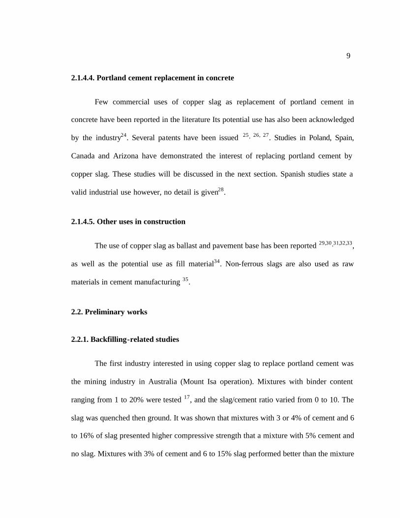
Since iron is the heaviest element in copper slags, it is tempting to find a

correlation between iron oxide content and specific gravity. This relationship is

represented in Figure II-4. The regression coefficient for a linear regression is equal to

0.94.

Figure II-4. Relationship between iron oxide content and specific gravity

2.5

2.7

2.9

3.1

3.3

3.5

3.7

3.9

0 10 20 30 40 50 60 70 80 90

Fe2O3 content (%)

21

2.6.1.2. Particle size distribution

The particle size distribution was determined by using an ATM sonic sifter, a

stack of sieves subjected to a high frequency acoustic vibrating motion. The high

frequency vibration enables use sieves with apertures smaller than the conventional

sieves. The particle size distribution of the representative sample of slag is shown in

Figure II-5.

Figure II-5. Particle size distribution of copper slag

0 100 200 300Particle Size, microns

0

20

40

60

80

100

Perc

ent P

assi

ng

22

2.6.1.3. Blaine fineness

The fineness of the copper slag was measured according to ASTM Standard C

204 using the Blaine air permeability test. As required by the standard, the constant “b”

used in the calculation of the value of the fineness, is to be determined for all materials

different from portland cement. In the case of the copper slag, the value of “b” was found

equal to 0.903. The average Blaine fineness of two replicate samples was 2700 cm2/g. In

order to compare the fineness of the slag to that of portland cement, the area of the grains

per unit of volume (intrinsic value) instead of the area per unit of weight (whose value

depends on the specific gravity) must be calculated. One would obtain a specific surface

area of 9450 cm2/cm3 for the slag and 10,900 cm2 /cm3 for a typical Type I Portland

Cement (Blaine fineness : 3460 cm2/g) ; indicating that both materials are in the same

range of fineness.

2.6.2. Chemical composition

The chemical composition, determined by the means of an electron microprobe

(average of 10 points), is indicated in Table II-2, along with the composition of other

copper slags from the literature.

23

Table II-1. Chemical composition (in % weight) of different copper slags

Source Origin Cu CuO SiO2 Fe2O3 MnO CaO MgO Al2O3 S SO3 LOI from[49] Copper Queen 1.35 15.9 64.2 0.3 7.0 1.1 10.0 0.2

Detroit 24.9 51.9 5.8 7.3 1.7 8.4 Prince 1.15 19.1 54.1 0.3 12.3 2.5 10.3 0.2 Old Dominion 2.36 17.1 71.5 1.0 3.2 1.6 3.3 United Verde 0.12 1.79 24.7 58.2 9.0 0.5 5.7 Bisbee 0.25 21.7 50.0 7.0 21.0

from [50] U.S.A. 0.4 29.3 57.0 0.05 3.8 0.8 4.0 from [5] Quebec 0.4 34.5 49.5 0.1 2.2 1.5 6.6 1.2 -5.2

Quebec 0.4 36.8 50.0 0.09 1.9 1.5 7.2 1.1 -6.1 Ontario 1.1 26.5 60.1 0.1 2.1 1.6 3.7 1.3 -5.9

from [28] Spain 0.93 18.4 76.9 0.02 0.32 0.01 3.0 0.50 -5.4 from [43] Poland 43.1 13.4 19.3 5.6 15.8 0.65 0.05 from [23] Taiwan 34.3 53.7 7.9 0.94 3.8 3.78 from [51] smelter 0.29 24.4 67.0 3.1 4.5 0.7

converter 1.76 15.8 78.2 0.4 2.9 0.9 Present study 0.65 35.2 52.8 0.03 3.3 0.57 5.0 2.46 -4.57

Note 1: negative LOI values indicate a gain due to oxidation of sulfur and iron oxide FeO. Note 2: analytical methods used in the cited references may be different from the one used in the present study. Some authors indicate that their results were obtained through wet chemical analysis.

Iron oxide is the major component of copper slags, silica being the second most

important. The sum of iron, silicon, aluminum, calcium, and magnesium oxides

constitutes 95% or more of the total oxides The copper slag studied here does not present

any singularity when compared with most of the copper slags of other origins.

It is possible to compare the chemical composition of copper slags with that of

iron blast-furnace slags, on a ternary diagram (CaO+MgO+Al2O3)-SiO2-Fe2O3 52. The

copper slag studied here is represented on this diagram (see Figure II-6).

24

Figure II-6. Representation of slags in the system (Cao+MgO+Al2O3)-SiO2-Fe2O3 (after

52)

CaO +MgO +Al2O3

Fe2O3

SiO2

20

20

20

40

40

40

60

60

60 80

80

80 steel slags

non-ferrous slags

copper slag

25

2.6.3. Mineralogical composition

Qualitative X-ray diffraction has been used for mineralogical characterization.

2.6.3.1. X-ray diffraction study

X-ray diffraction is based on Bragg’s law53, which describes the interaction

between a radiation and a geometrically organized arrangement of atoms (crystalline

lattice):

, = θλ sind2

where λ is the wavelength of the incident radiation,

θ is the angle of incidence,

and d the spacing between crystalline planes.

When the so-called powder method is used, the wavelength λ is kept constant

whereas the angle of incidence θ is variable. When θ reaches a value that verifies Bragg’s

law, the intensity of the diffracted radiation passes by a maximum (peak). Each peak

corresponds to a value of d-spacing. Every crystalline structure is characterized by a set

of d-spacings, corresponding to all the crystalline planes. The ICDD database contains

the values of the d-spacings of all known crystals, along with the relative intensity

expected for each peak, with respect to the strongest peak. Therefore, interpreting a XRD

26

diagram is a matter of finding in the database which crystal(s) correspond(s) to the

recorded peaks.

As underlined above, XRD gives optimal results in term of characterization when

crystalline components are analyzed. In the case of glassy materials, where atoms adopt a

much less organized structure, the XRD diagram presents the shape of a broad hump

(halo) which displays a maximum corresponding to the most probable spacing between

atoms 53. When a component is partly crystalline, partly glassy, the diagram is made of a

halo surmounted by a set of peaks. Granulated (quenched) iron blast- furnace slags are

mostly glassy, thus present either a single-halo diagram or a halo-and-peaks diagram 4.

The XRD pattern obtained for the total fraction of the copper slag of the present

study is presented in Figure II-7.

27

Figure II-7. XRD pattern of studied copper slag

XRD patterns have also been generated for 3 separate dimensional fractions: less

than 45 µm (Figure II-8), 45 µm to 75 µm (Figure II-9), greater than 75 µm (Figure II-

10).

28

Figure II-8. XRD pattern of fraction less than 45 µm

Figure II-9. XRD pattern of 45 µm to 75 µm fraction

29

Figure II-10. XRD pattern of fraction greater than 75 µm

The observed peaks correlate well with the reference patterns for Fe3O4

(magnetite), and Fe2SiO4 (fayalite) as the main phases present in the slag. Although

aluminum has been detected in notable proportion by the chemical analysis, no

aluminum-bearing component has been identified by the XRD method. This is possibly

due to the fact that the peaks of fayalite are intense and in great number, thus may hide a

minor constituent.

The slag used in the present study appears to be well crystallized, which is

consistent with its mode of cooling (air-cooling). The X-ray diffraction pattern does not

display the usually broad halo of the high glass-content slags. One can also note that the

30

background radiation is fairly high, which is due to the fluorescent radiation emitted by

the important proportion of iron in the slag, excited by the Cu Kα1 radiation.

The absence of a glassy halo in non-ferrous slags, even though glass may be

present, has also been noted in the literature 37. Consequently, it was not possible to

determine the glass content of the present slag by using the methods based on XRD 54,55.

Other methods exist, based on image analysis of SEM or optical micrographs 5,56,57.

2.6.3.2. Raman spectroscopy study

Since conventional methods did not enable us to determine the absence or

presence of glass, another type of characterization device was used: Raman spectroscopy.

Similar to Infrared spectroscopy, Raman spectroscopy is based on the analysis of the

interaction of light with the molecules of a material 58. But, whereas Infrared

spectroscopy is related to the absorption of light by the molecules, Raman spectroscopy

deals with the scattering of the light beam by the bonds within molecules. This

phenomenon involves a change in wavelength of the incident radiation. This change is

recorded and is correlated to a given bond in a molecule. A laser provides the incident

monochromatic beam. The scattered radiation is diffracted by a grating then analyzed by

a CCD camera 59. Powders or single crystal samples can be analyzed. The method is

applicable to minerals 60.

When crystalline materials are analyzed by Raman spectroscopy, the

corresponding spectra are made of peaks, because of the periodicity of the structure.

31

Glasses provide broad humps, since here bonds are aperiodic61, 62 . The Raman spectrum

corresponding to the copper slag studied in this work is presented in Figure II-11. This

spectrum displays only peaks, which means that the material is mostly in a crys talline

form.

Figure II-11. Raman spectrum of studied copper slag

2.6.3.3. Conclusion

The copper slag presently does not seem to exhibit a very glassy structure. The

hydraulic potential of a blast- furnace slag is related to its physical state, i.e. crystalline or

amorphous 63. When a blast- furnace slag is entirely in crystalline form, it is said that it

-1000 -500 0 500 1000 1500 2000 2500

Wave number (cm-1)

32

has “no or only very weak hydraulic or latent hydraulic” 64. It has also been shown that,

when used in mortars with portland cement:

q fully glassy slags do no t lead to the highest mortar strength and

q slags containing 35% of crystalline phase exhibit a strength comparable to slags

containing 5% of crystalline phase 56.

Similar conclusions have been drawn by other autho rs 57, 65, although they do not

concern non-ferrous slags.

2.6.4. Study of copper slag/ lime pastes

2.6.4.1. Methodology

The purpose of studying slag/ lime pastes is to better understand the reaction

between one of the hydration products of portland cement, calcium hydroxide, without

the interference of the other compounds. Such reaction is characterized by the decrease of

the quantity of calcium hydroxide and the formation of an hydration product.

In a previously cited study 36, non-evaporable water measurements and semi-

quantitative XRD have shown that a maximum quantity of hydration products was

formed for slag/calcium hydroxide pastes containing 90 to 95% slag.

Two series of pastes were investigated:

33

q Pastes containing 95% copper slag and 5% lime, prepared with a water/solid ratio of

0.23.

q Pastes containing 85% copper slag, 10% activator (see 2.5), and 5% lime prepared

with a water/solid ratio of 0.29. Tap water was used to prepare the pastes.

The difference in water/solid ratio stands for the goal of obtaining a comparable

consistency for the two series. Three identical replicates of each series were prepared

After mixing, the samples were cast in small plastic containers and stored in a

23°C temperature and 100% RH atmosphere.

The specimens were examined at 1, 2, 7, 14, 28, 56, 90 and 180 days by X-ray

diffraction. The so-called “semi - quantitative method”, based on the premise that the

quantity of a component is proportional to the intensity of its diffraction peaks, was used

here. In that method, after the nature of the components has been determined (qualitative

analysis), the intensity of the most interesting diffraction peaks is measured for each

testing time. Then, the relative intensity of these peaks is computed by dividing their

intensity I(t) by the intensity of the peak of an internal standard I0(t) (belonging to the

sample studied) or external standard (introduced in the sample) corresponding to an inert

component whose quantity remains constant with time (see Figure II-12). Such a

procedure is necessary because the characteristics of the XRD installation may vary with

time, which means that the intensity of the peaks corresponding to an inert mineral, thus

its quantity, may appear to vary with time, only because of variable equipment

34

conditions. The computation of the relative intensity enables one to cancel out these

variations. Obviously, this method indicates only the variation with time of the relative

quantity of a given component. But this is appropriate in the case of the study of the

kinetics of hydration reactions, since one is interested in:

q components whose quantity is maximum at the origin of time: non-inert

components forming the initial sample, and

q components whose quantity is equal to zero at the origin of time: hydration

products.

Figure II-12. Principle of XRD semi-quantitative method

In the present case, the only non- inert component in the slag/lime pastes (in the

absence of activator) is the calcium hydroxide present in the lime. The complexity of the

problem is that the most intense peaks of calcium hydroxide (d =4.900 Å, 2.628 Å, 1.927

Å1) correspond to spacings close to fayalite (d =2.633 Å, d =2.619 Å, d =1.922 Å2) or

1 JCPDS-ICDD data sheet n°4.733 2 JCPDS-ICDD data sheet n°34.178

I0(t)

I(t)

35

magnetite (d =4.852 Å 3) peaks. Therefore, the intensity of calcium hydroxide peaks is

compounded with the intensity of the peaks of these inert crystalline phases. The other

peaks of calcium hydroxide are too weak and/or hidden by other peaks of fayalite or

magnetite. Thus, the following methodology has been applied:

q computation of the average relative intensity of some major fayalite peaks, for the

three replicates with the internal standard being the most intense fayalite peak (d

=2.500 Å). These peaks are chosen not to correspond with calcium hydroxide peaks

except one (d =2.633 Å).

q plotting of these relative intensities versus time. If the amount of calcium hydroxide

would decrease, the relative intensity of the 2.633 Å peak would decrease also, but

the relative intensities corresponding to the other fayalite peaks should remain

constant.

The ratio of the intensity of the 2.63 Å peak to other inert mineral peaks (fayalite

d = 2.829 Å and magnetite d = 2.532 Å) peak was plotted against time, to confirm the

variation of that compounded peak.

3 JCPDS-ICDD data sheet n°19.629

36

2.6.4.2. Results for pastes without activator

The variation with time of the relative intensity of different fayalite peaks is

described by Figure II-13.

Figure II-13. Copper slag/lime pastes without activator. Variation with time of the

relative intensity of fayalite (F) peaks

It is shown by this figure that only the intensity of the 2.63 Å peak decreases slightly

from about the age of 28 days whereas the other ratios remain constant. This means that

the quantity of calcium hydroxide decreases, which is indicative of a reaction between

2 3 4 5 6789 2 3 4 56789 21 10 100

Time, Days

0.0

0.4

0.8

1.2

1.6

Rel

ativ

e In

tens

ity

F3.97/F2.5

F2.84/F2.5

F3.56/F2.5

F2.63/F2.5

37

slag and calcium hydroxide. This is confirmed by the study of the ratio of the intensity of

the 2.63 Å peak to other inert minerals peaks, as shown by Figure II-14.

Figure II-14. Copper slag/lime pastes without activator. Variation with time of the

relative intensity of the 2.63 Å peak to fayalite (F) 2.829 Å, 2.500 Å and magnetite (M)

2.532 Å peaks

However, no hydration product has been detected, possibly because of the great

number of peaks of inert minerals, which may have hidden its peak (if it is a crystalline

hydrate). It should also be noted that this reaction is not very intense.

2 3 4 5 6789 2 3 4 5 6789 21 10 100

Time, Days

0.0

0.2

0.4

0.6

Rel

ativ

e In

tens

ity

F2.63/F2.5

F2.63/M2.53

F2.63/F2.84

38

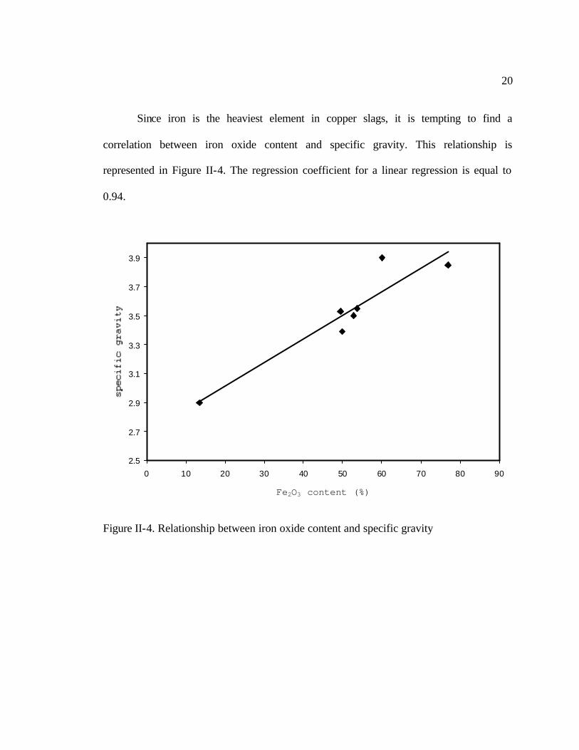
Figure II-15 and Figure II-16 display typical XRD patterns of slag/lime pastes at 1

day and 180 days.

Figure II-15. XRD pattern of slag/lime pastes at 1 day

39

Figure II-16. XRD pattern of slag/lime pastes at 180 days

2.6.4.3. Results for pastes with activator

The variation with time of the relative intensity of fayalite peaks is described by

Figure II-17.

40

Figure II-17. Copper slag/lime pastes with activator. Variation with time of the relative

intensity of fayalite (F) peaks

As for the pastes with activator, it is shown by Figure II-17 that only the intensity

of the 2.63 Å peak decreases whereas the other ratios remain constant. This observation

indicates a reaction between slag and calcium hydroxide. This is also confirmed by the

study of the ratio of the intensity of the 2.63 Å peak to other inert minerals peaks, as

shown by Figure II-18.

2 3 4 5 6789 2 3 4 5 6789 21 10 100

Time, Days

0.0

0.4

0.8

1.2

1.6

Rel

ativ

e In

tens

ity

F3.97/F2.5

F2.84/F2.5

F3.56/F2.5

F2.63/F2.5

41

Figure II-18. Copper slag/lime pastes with activator. Variation with time of the relative

intensity of the 2.63 Å peak to fayalite (F) 2.829 Å and magnetite (M) 2.532 Å peaks

Again, no hydration product has been detected, and it can be noted that the

reaction is not very intense, despite the presence of the activator. Figure II-19 and Figure

II-20 display typical XRD patterns of slag/lime pastes with activator at 1 day and 180

days.

2 3 4 5 6789 2 3 4 5 6789 21 10 100

Time, Days

0.0

0.2

0.4

0.6

Rel

ativ

e In

tens

ity

F2.63/F2.5

F2.63/M2.53

F2.63/F2.84

42

Figure II-19. XRD pattern of slag/lime pastes with activator at 1 day

Figure II-20. XRD pattern of slag/lime pastes with activator at 180 days

43

2.6.5. Study of copper slag/ portland cement pastes

2.6.5.1. Methodology

In the case of portland cement /copper slag pastes, it is interesting to study not

only the rate of formation of calcium hydroxide formed by the hydration of the cement,

but also the rate of disappearance of some of the main compounds which constitute the

anhydrous cement. To investigate the effect of the copper slag on the hydration process

of the portland cement, a paste blend of 85% portland cement and 15% copper slag was

compared to a paste made up of 100% portland cement. A water to cement ratio of 0.34

was used for both mixtures. After mixing, the samples were cast in small plastic

containers and stored in the same conditions as the slag/lime pastes. Three replicates of

each mixture were studied at 2, 7, 14, 28 and 56 days of curing.

To monitor the rate of formation of calcium hydroxide, which is called

portlandite when it is the result of portland cement hydration, two methods have been

used:

Using semi-quantitative XRD, the intensity of the d =2.500 Å fayalite peak

present in the cement/slag pastes patterns was used as reference for both two types of

pastes in order to offset the time variability of the XRD installation. The intensity of the

peaks obtained for the slag/cement pastes was corrected to match the intensities of the

100% cement pastes. The d= 2.629 Å peak has been used for the portlandite; as seen

previously, this peak is augmented by the d= 2.633 Å peak of fayalite in the case of the

44

slag/cement pastes. But since only 15% of slag are present in these mixtures, and since

this fayalite peak is not very intense, the effect of this peak in the value of the resultant

has been neglected. This tends to slightly overestimate the amount of portlandite.

Thermogravimetry analysis (TGA) enables determination of the amount of water

bound in portlandite, and the total amount of chemically bound water. Thermogravimetry

analysis consists of the recording of the loss of weight of a sample being progressively

heated up to a constant weight. In the case of cementitious hydrated materials, weight

loss is due mainly to mineral decomposition and evaporation of the total chemically

bound water (considered from 105°C to 900°C). The amount of water bound in

portlandite is determined by the step between 425°C and 550°C measured from the loss

of weight – temperature curves 66’ 67. The slope and the intercept of the tangent at 550°C

are computed by linear regression, and the water bound in portlandite is obtained by the

difference of weight loss between 425°C, read on the curve, and the ordinate of the

tangent for 425°C. Figure II-21 describes this procedure. The weight loss magnitudes

were normalized based on the weight of raw cement in the reference specimens (100%

portland cement pastes).

45

Figure II-21. Procedure for determination of water bound in portlandite (after66)

Whereas TGA was used to study the hydrates formed, the anhydrous components

of portland cement were analyzed using semi-quantitative XRD. The d=2.74 Å peak,

common to both alite and belite, has been used to monitor the decrease of the anhydrous

calcium silicates using also the d=2.500 Å fayalite peak intensity as reference. Alite

(C3S) and belite (β-C2S) make up about 75% of this type of cement and determine most

of the properties of the hydrated cement paste.

400 500 T °C

weight loss

step

46

2.6.5.2. Results

The process of formation of portlandite, monitored through semi-quantitative

XRD is described in Figure II-22. In this figure, the solid lines correspond to the average

of the three replicates and the dashed lines to the confidence interval for a level of

confidence of 95%. It can be seen that no significant difference in portlandite formation

between cement pastes with and without slag can been detected.

Figure II-22. Variation of portlandite in cement/slag pastes

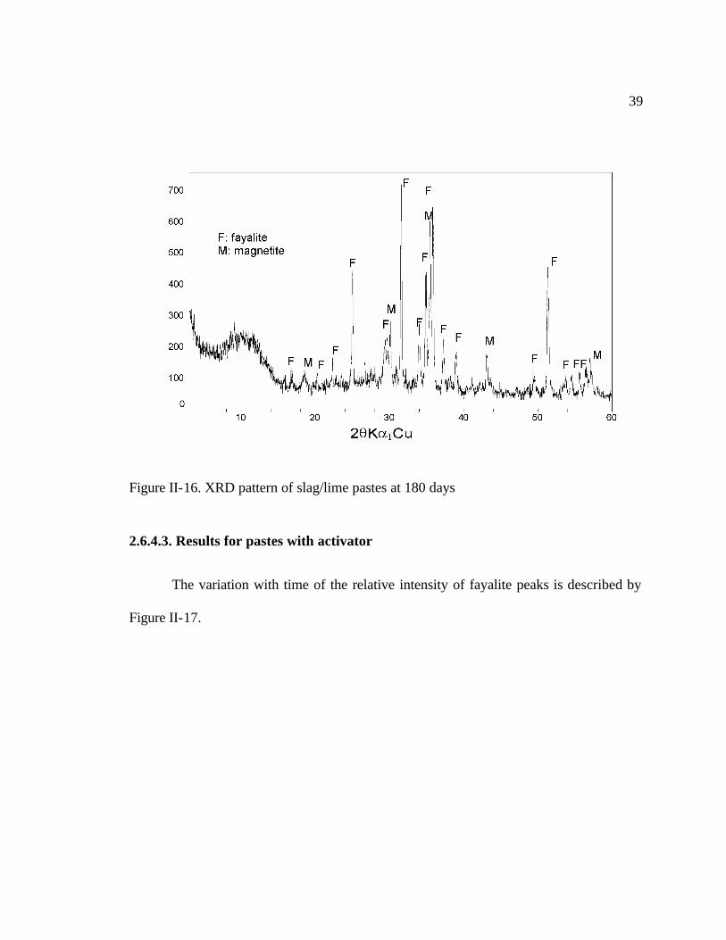
In a similar manner, the variation of the relative quantity of alite/belite is

indicated in Figure II-23. Again, it is not possible to distinguish a difference between

0 20 40 60Time, Days

4

6

8

10

Rel

ativ

e In

tens

ity

100 % cement

85 % cement / 15 % slag

47

plain cement and slag blended cement. This is consistent with the conclusion relative to

the formation of portlandite since this hydrate is formed only by both alite and belite.

Figure II-23. Variation of the relative quantity of alite/belite in cement/slag pastes

0 20 40 60Time, Days

0

1

2

3

4

Rel

ativ

e In

tens

ity

100 % cement

85 % cement / 15 % slag

48

Figure II-24 and Figure II-25 display typical XRD patterns of 100% cement and

85% cement / 15% copper slag pastes at 56 days.

Figure II-24. XRD pattern of 100% cement paste at 56 days

49

Figure II-25. XRD pattern of 85% cement - 15% copper paste at 56 days

Data obtained from thermogravimetry analysis are reported in Figure II-26 and

Figure II-27.

50

Figure II-26. Variation with time of the amount of water bound in portlandite

0.0

0.5

1.0

1.5

2.0

2.5

3.0

time (days)

100 % OPC

85 % OPC - 15 % slag

2 7 14 5 6

51

Figure II-27. Variation with time of the total amount of chemically bound water

Although at early age the presence of copper slag seems to accelerate the

hydration of portland cement slightly (more portlandite is detected and the amount of

bound water is higher), long-term values of the total chemically bound water are

comparable in pastes with and without slag, which indicates that the copper slag has little

influence on the long-term hydration of the cement. The slightly lower amount of

portlandite at long-term in the cement-slag paste, compared to the cement-only paste

seems to indicate a weak reaction between slag and calcium hydroxide, as noted in the

study of the pastes slag/lime. Nevertheless, the amount of calcium hydroxide does not

0

5

10

15

20

time (days)

100 % OPC

85 % OPC - 15 % slag

2 7 14 5 6

52

appear to decrease, because the weak reaction of consumption of calcium hydroxide by

slag may be offset by the slow yet continuing formation of this hydrate by the cement

after 28 days 68.

The weight of loss curves for the TGA analysis are reported in Figure II-28,

Figure II-29, Figure II-30, and Figure II-31.

Figure II-28. Weight of loss curves of cement and cement/slag pastes at 2 days

0

5

10

15

20

25

0 200 400 600 800 1000

temperature (degrees C)

100 % cement

85 % cement - 15 % slag

53

Figure II-29. Weight of loss curves of cement and cement/slag pastes at 7 days

0

5

10

15

20

25

0 200 400 600 800 1000

temperature (degrees C)

85 % cement - 15 % slag

100 % cement

54

Figure II-30. Weight of loss curves of cement and cement/slag pastes at 14 days

0

5

10

15

20

25

0 200 400 600 800 1000

temperature (degrees C)

85 % cement - 15 % slag

100 % cement

55

Figure II-31. Weight of loss curves of cement and cement/slag pastes at 56 days

2.7. Conclusions

The potential use of ground copper slag as a mineral admixture for concrete has

been studied, from the viewpoint of characterization and effect on cement hydration

properties.

By different characterization methods, it was found that the copper slag studied is

mainly a crystalline material, made up of the minerals fayalite and magnetite. This type

of composition is typical of air-cooled non-ferrous slags.

0

5

10

15

20

25

0 200 400 600 800 1000

temperature (degrees C)

85 % cement - 15 % slag

100 % cement

56

The monitoring of lime-copper slag pastes indicates that, at long term, the

quantity of available calcium hydroxide decreases, indicating a possible pozzolanic

reaction. The use of an activator did not enhance this reaction. Such a reaction was not

detected for portland cement-copper slag pastes. Nevertheless, past studies show a

reduction in the capillary porosity by the copper slag grains. This leads to an increase in

strength and durability of mortars and concrete with copper slag as a mineral admixture,

possibly improved by the minor pozzolanic properties.

CHAPTER 3

MODELING OF DAMAGE DUE TO EXPANSION IN BLENDED

CEMENT MORTARS SUBJECTED TO EXTERNAL SULFATE ATTACK

3.1. Introduction

As mentioned in Chapter 2, previous studies have shown that the replacement of

cement by copper slag in mortar improves the resistance to external sulfate attack. The

effects and causes of this durability problem have been extensively investigated for

decades (beginning in the XVIIIth century69), since it is responsible for the degradation of

a large number of structures worldwide. Nonetheless, “the literature on sulfate attack is

complex and confusing” and “the mechanisms by which the various external sulfates

attack concrete are still a matter of some controversy” 70.

Internal sulfate attack, such as delayed ettringite formation, is not considered in

this chapter. Although another form of internal sulfate attack has been called “secondary

ettringite formation”71, the term “secondary ettringite” will be used here to qualify

ettringite formation due to external sulfate attack.

The main reported vectors responsible for transport mechanism of sulfates are

groundwater72, sewage water, industrial solutions, or polluted atmospheric air73. The

sulfates contained in sea water do not appear to be directly responsible of

degradation74,75, although the sulfates concentration is high; harmful actions for concrete

in marine environment are due to dissolved carbon dioxide and magnesium ions, with

chloride ions leading to reinforcement corrosion. Although secondary ettringite is formed

58

due to sulfates ingress, it is said that the presence of chloride ions hinders its expansion

(due to binding of calcium aluminates in Friedel’s salt). Nevertheless, cracks filled with

ettringite have been observed in field concrete exposed to sea water76.

The nature of and concentration of sulfates present in the aggressive agents is

very variable. The cations associated with sulfates can be calcium, magnesium, sodium,

ammonium or potassium, magnesium being the most destructive77,78. Concentration

levels of 150 ppm and higher are considered aggressive and require mitigation, with more

drastic precautions as the concentration increases 79. Typical concentration level of

sulfates in tap water is of the order of 400 ppm in Phoenix, AZ.

The magnitude of the concrete durability problem and the extent of degradation

due to sulfate attack may be directly related to the composition of the material and its

subsequent physical characteristics (pores system, permeability80,81 and strength). The

pore size distribution of the hardened cement paste, which is the matrix of the concrete, is

made up of “capillary pores” and “gel pores”82. The proportion of capillary pores is more

important in normal strength concrete than in high-strength concrete, which determines

the higher permeability of the former. Composition parameters include nature and dosage

of cement, presence of mineral admixtures, water/cement ratio, mode of curing. The role

of the microstructure of the aggregate/paste zone 83,84 and the influence of the

mineralogical nature of the aggregates85 have also been studied.

The mode of exposure of sulfates with concrete is also very important: cyclic

wetting-drying exposure can be more harmful than continuous soaking8687.

59

Corrosion of reinforcement steel bars by chlorides is accelerated when sulfates

have also ingressed88, resulting in the overall damage of the structure.

A single widely recognized test to assess the sulfate resistance of concrete does

not exist yet. However, one can distinguish two broad families:

q tests based on the measurement of the expansion of mortar89 or concrete

specimens90,

q tests determining the loss of strength91 (through mechanical or ultrasonic

tests).

For a given test procedure, the difficulty lies in the determination of an acceptance

criterion with respect to field conditions 92. Many procedures utilize a 0.1% expansion

threshold as the limit, but this level is quite arbitrary based on service record.

Since expansion appears to be the main phenomenon in the case of sodium sulfate

attack, and loss of strength the one in case of magnesium sulfate attack, it is suggested

that the corresponding tests be applied taking into account the nature of the cations 93. But

the same study points out that, depending on the nature of the binder, the amplitude of the

concomittant phenomenon can greatly vary 94.

Other tests include the measurement of the weight change of the specimens, for

example during soaking-drying cyclic tests 95.

60

3.2. Effects of sulfate attack on concrete microstructure

Depending of the nature of the associated cation77 two principal phenomena are

observed to occur. These mechanisms may or may not occur concurrently when concrete

is attacked by sulfates:

q expansion followed by cracking and disintegration,

q softening and decomposition,

Cracks often occur parallel to the surface of the concrete, but also at the

aggregate/paste interface. They are often filled with gypsum and/or ettringite. These

minerals can be identified by optical microscopy or SEM 96, using standard petrographic

techniques.

Removal of successive layers (of a specimen subjected to sulfate attack) and

analysis of the resulting surfaces has shown the presence of gypsum, then ettringite, then

monosulfate, from the surface towards the core of the specimen, with decrease of the

quantity of portlandite observed from the core towards the surface97; decalcification of C-

S-H was demonstrated by X-ray microanalysis. Ettringite formation, leading to

expansion, does not seem to occur necessarily at aluminates sites, but in a more diffuse

manner throughout in the microstructure98.

When magnesium sulfate is involved, decalcification of C-S-H corresponds to the

formation of M-S-H (magnesium silicate hydrate) which does not have cementitious

properties99.

61

Subsequent loss of resistance of the matrix due to this type of deterioration was

often shown indirectly by measurement of the loss of strength of specimens, or by micro-

hardness measurements100. The effect of cracking and/or leaching of calcium may lead to

an increase of the permeability 101 and diffusivity102.

The complexity of the physico-chemical mechanisms observed in permeable

structural concrete sub jected to sulfate-bearing groundwater ingress and evaporation, has

been recently exposed. Bands of gypsum form parallel to the surface exposed to the soil,

ettringite is associated to local cracking, portlandite and C-S-H are decalcified, as well as

unhydrated alite and belite, and new minerals crystallize in the subsequent gaps103,104.

The presence of magnesium silicate, brucite, Friedel’s salt and sodium carbonate show

that many types of ions are transported through the porous structure and react with the

cement paste105.

A simplified cracking mechanism of mortars exposed to a sodium sulfate solution,

has been proposed based on microstructural observations. Ettringite forms in the surface

layer, which leads to cracking in this layer and to a lower amount of cracking in the

subsequent layers into which sulfate ions have not ingressed yet; then, when ettringite is

formed in this second layer, it induces cracking in the next non- invaded layer, whereas its

own expansion is being restrained by the presence of the third layer 106.

In a laboratory case of magnesium sulfate attack, it has been observed gypsum

deposits form within the material in layers parallel to the surface, while there is a brucite

layer at the surface. Meanwhile, ettringite was formed in very small quantities 107,108.

62

A less frequent and different form of sulfate attack occurs in cases when the

temperature is cold (5 to 15°C) and carbonate ions are present109. The mechanism

involves the rapid breakdown of C-S-H, which leads to total decomposition of the

hydrated cement paste. Silicates from C-S-H, and carbonates are involved in a new

compound called thaumasite.

Other forms of attack involving sulfates are 110:

q degradation caused by expansive crystallization of sulfate salts at the surface

of the concrete when water evaporates111,

q naturally occurring sulfitic minerals forming sulfuric acid whose pH is low

enough to attack concrete, with symptoms resembling “conventional” sulfate

attack.

3.3. Physico-chemical mechanisms involved in sulfate attack

To simplify the problem, two types of chemical reactions, which are linked, are

believed to occur as sulfate ions ingress in concrete:

q Decomposition or alteration of calcium-based hydrates, portlandite and C-S-H

(decalcification reactions), due to removal or substitution of calcium ions

from the structure of these hydrates.

q Formation of expansive products from calcium aluminates, hydrated or not

(expansion-type reactions). Expansion is attributed to the lower specific

63

gravity of the newly formed ettringite, compared to the initial reactants. The

validity of this one and other ettringite-related mechanisms have been

analyzed, none of them has been deemed fully satisfactory to explain

expansion112. Expansion causes distresses such as cracking and spalling. The

network of cracks formed is a path for aggressive agents to further invade the

structure.

In this chapter, only the expansion-type reactions will be considered. This

hypothesis states that compared to the original compounds, expansion is due to the much

lower specific gravity of ettringite,.

3.3.1. Compounds present in hydrated cement paste

To describe the reactions taking place during sulfate attack, it is necessary to

establish the constitution of the compounds originally present in the hydrated cement

paste. C2S and C3S form portlandite and C-S-H. C3A can lead to the following

reactions 113, depending on the conditions (such as gypsum content in cement and

water/cement ratio):

q Formation of tetracalcium aluminate hydrate, according to the reaction:

1343 12 AHCHCHAC →++

q Formation of ettringite, (referred as primary ettringite, as opposed to the

secondary ettringite due to sulfate attack):

64

ettringite gypsum H S A C HHS3C AC 323623 →++ 26

q Conversion of primary ettringite into calcium aluminate monosulfate hydrate,

most often referred as “monosulfate”, following the reaction:

If the two previous reactions are added up, the transformation of C3A to

monosulfate is given by:

emonosulfat gypsum H S A C HHSC AC 12423 →++ 10

Also, some C3A may have not reacted as is referred to as residual C3A. C4AF

hydration corresponds to similar reactions, with iron-bearing hydrates and amorphous

phases114.

3.3.2. Expansion reactions

The expansion-type reactions are originated from the combination between

portlandite and ingressing sulfate ions, which leads to the formation of gypsum, as for

example with sodium sulfate77 :

Ca(OH)2 + Na2SO4.10H2O → CaSO4.2H2O + 2 NaOH + 8 H2O

emonosulfatettringiteH S A C 34H ACH S A C 12433236 →++ 2

65

Then, gypsum can react with tetracalcium aluminate hydrate, monosulfate or

residual C3A to form expansive ettringite, according to the following equations,

expressed in shorthand cement chemistry notation (see Chapter 2):

CHH S A C 14H HSC 3AHC 32362134 +→ ++

32362124 H S A CH16HSC2H S A C →++

323623 H S A C H26HS3C AC →++

Another mechanism has been suggested, that the attack occurs first on C4AH13,

with direct formation of monosulfate and ettringite, followed by formation of gypsum

from portlandite115,116.

Another school of thought proposes that the formation of ettringite itself is not

expansive, but that this compound has a colloidal structure that can adsorb significant

quantities of water, which causes expansion 117,118,119,120.

Previously, it was thought that gypsum is formed during a through-solution, thus

this formation would not induce a volume increase. Although the question is debated, it

has been shown recently, using alite paste and mortar, that the formation of gypsum itself

also causes expansion121,122.

3.4. Mitigation of sulfate attack

Techniques to prevent sulfate attack of concrete include:

66

q Coating of the surface to stop ions ingress 123,124.

q Design of very compact, well cured concrete125,126.

q Use of so-called calcium sulfoaluminate cements (based on SAC 34 )127.

q Use of a cement with low C3A content 128,129,130,131 (for example ASTM type II

and V cements). In this type of cement, C3A is partially replaced by C4AF,

this compound being much less sensitive to sulfate attack. Nonetheless, the

ratio C3S/ C2S is also an important parameter since C3S produces more

portlandite than C2S 132. It has been emphasized that the use of so-called

sulfate-resistant cement should be concomitant with sound physical properties

for the mix design, such as low permeability133. Also, because residual C4AF

and/or C4AF hydration products may be also responsible for sulfate attack, but

at a slower rate than C3A, a standard limit has been imposed on the total

amount of calcium aluminates in cement, expressed as 2×[C3A]+[C4AF]134.

q Partial replacement of cement by mineral admixtures135,136, such as natural

pozzolans 137, fly ash138,139,140, silica fume 141,142,143,144, thermally treated clay145

,rice husk ash146, or blast-furnace slag147,148,149,150 . The use of admixtures has

multiple beneficial effects:

• Dilution of C3A, since less cement is present.

• Reduction of the amount of portlandite, for the same reason.

67

• Further reduction of the amount of portlandite, when consumed by the

pozzolanic reaction.

• Reduction of permeability, due to better packing and/or formation of

denser hydrates.

Slag cements, in which blast- furnace is the dominant component and portland

clinker the minor component, are another alternative. The sulfate resistance of

such cements, from the secondary ettringite formation point of view, is linked

to the aluminate content of the slag, the slag content in the cement, and the

amount of sulfates added originally to the anhydrous cement151. Nevertheless,

softening due to decalcification of C-S-H is the driving cause of their

degradation152. It is not clear whether slag cements display a higher sulfate

resistance than low C3A- portland cements or not 153,154.

Studies of slag cements pastes (and high volume fly ash cement pastes), with

low water/solids ratio (0.26 to 0.28), exposed to sulfates-bearing groundwater,

have shown that very little ettringite or gypsum has formed, which is

attributed to the low permeability of the materials. But ettringite and gypsum

were found in large amounts in cracks pre-existing in some specimens 155.

The use of admixture may reduce the resistance to sulfate attack, for some

high-calcium fly ashes156. The beneficial use of silica fume has been

somewhat questioned 157,158,159 , especially is the case of magnesium sulfate

68

attack. A particular case of slag cement is the “supersulfated cement”, which

may contain up to 15% of gypsum, and was proved to be very effective in

term of sulfate resistance4.

3.5. Modeling of sulfate attack

The principal effect of sulfate attack is to reduce the service life of the concrete

structures due to degradation. The ultimate goal of modeling of sulfate attack is to predict

the service life of a structure given the environmental conditions and the characteristics

of the structure and the concrete.

3.5.1. Literature review

Several models for sulfate attack have been devised by researchers using

approaches based on different scientific fields: engineering, mechanics, physics and

mathematics. This diversity in approach may explain the different assumptions and the

various mechanisms considered.

The project of disposal of low-level radioactive nuclear wastes in buried concrete

vaults160 has led to the question of the long-term durability of the concrete. One model

proposes that the rate of spalling be expressed as a function of the elastic and fracture

properties of concrete, its intrinsic sulfate diffusion coefficient, the external sulfate

concentration and the concentration of ettringite161, based on an empirical relationship

between ettringite formation and expansion162. The expansive strain is linearly related to

the concentration of ettringite. This approach has been incorporated in the 4SIGHT

69

program, which predicts the durability of concrete structures163, 164 , as well as in a model

that calculates the service life of structures subjected to the ingress of sulfates by

sorption165.

Another approached is based on a general conservation equation involving

diffusion, convection, chemical reaction and sorption166, as phenomena governing the

transfer of mass through concrete. In the case of sulfates, the authors assume that the

process is controlled by reaction rather than diffusion, based on an empirical linear

equation that links the depth of deterioration at a given time to the C3A content and the

concentration of magnesium and sulfate in the original solutions. Quasi-steady state is

then supposed to be reached quickly, and the integration of the resulting differential

equation yields the theoretical position of the deterioration front as a function of time.

This result is being used in a further model that predicts the expansion167 of mortar bars,

using a logarithmic fit of the expansion versus time curves, and a fractal analysis of the

sulfate attack- induced crack network. The fractal dimension is tied to the “time order” of

the degradation, this parameter being characteristic of the rate of degradation168,169 . For

example, in the case of sulfate expansion, the time order is given by the slope of the

logarithmic fit of the expansion versus time curves. This approach is integrated in a study

of the different aggressive agents affecting the long-term durability of low level nuclear

waste concrete barriers170.

A solution of the diffusion equation with a term for first order chemical reaction

has been proposed to determine the sulfate concentration as a function of time and

70

space171,172, but the chemical composition of the cement does not appear to be taken into

account. The diffusion coefficient is considered as a function of the capillary porosity,

which varies with time because capillary pores fill up with the recently formed minerals.

No further attempt was made to predict durability parameters.

Clifton et al.. used the finite difference method to solve the diffusion equation

with first order chemical reaction, as applied to the reaction between sulfates and

portlandite173. The “random walkers method” has also been applied. Only concentration

profiles were devised.

Chemical and physical phenomena can be described by a general equation

expressing the variation of concentration of ionic species through a permeable

material174. The concrete is here considered as non-saturated. Effect of temperature is

accounted for. Different models for chemical and physical interactions terms are

reviewed175.

Stresses within the concrete can be computed assuming that a specimen subjected

to sulfate attack can be modelled as an elastic matrix containing expansive inclusions; the

simulation of the expansion of sites located within the surface of the specimen yields

random tensile stress fields compatible with the random crack network observed

experimentally252.

A computer program has been developed to determine the concentration of the

various species in building materials subjected to chemical attack, then the extent of the

71

distresses due to the chemical transformations 176, 177. The chemical calculations are based

on thermodynamical and kinetical considerations, and different modes of transport can be

adopted. The residual strength of the material is derived from a formula involving the

porosity, and the expansion from the amount of secondary ettringite formed and the pore

radius distribution. Expansion data are in good agreement with simulations.

Using micromechanics theory and the diffusion-reaction equation yields a

complex model that predicts the expansion of mortar bars178 has been developed for the

1-D case.

A pure mathematics study of coupled diffusion-reaction equations for gypsum

formation in concrete has been presented179.

From the molar volumes of the different components of the cement paste, and its

microstructural parameters (degree of hydration, capillary porosity), the expansion is

predicted, assuming no expansion occurs until the capillary pores are totally filled with

ettringite180. Depending on the type of secondary reaction, expansion may or may not

globally occur. It would appear that conversion of monosulfate is not always expansive.

3.5.2. Model proposed

3.5.2.1. Chemical interactions

The formation of ettringite from sulfates and calcium aluminates will be

simplified here as a second order homogeneous one-step reactions :

72

3236134 H S A C S 3AHC → +

3236124 H S A CS2H S A C →+

32363 H S A C S3 AC →+

To simplify, these reactions will be lumped in a single one:

3236 H S A C Sq CA →+

where “CA” signifies an equivalent grouping C4AH13, monosulfate and residual

C3A. The molar concentration in “CA” is the weighted average of the concentration of

the three components. Likewise, q represents the average stoechiometric coefficient of

the lumped reaction, obtained from the coefficients of the individual reactions (i.e.: 3, 2

and 3). The method to compute q is given in Appendix I.

The rates of reaction can be expressed as181,182:

U U k - dT

U d

ACSO

SO

4

4 =

q

U U k -

dTU d

ACSOAC 4=

with: U, molar concentration,

73

T, time,

k rate constant.

3.5.2.2. Diffusion and reaction

The case treated here is for a saturated concrete, indicating that sorption is not

involved183,184. The unsteady-state diffusion of sulfates ions will be considered obeying to

Fick’s second law185:

2

2

XU

DTU

∂∂

=∂∂

with:

U, concentration,

T, time,

X, distance,

D, diffusion coefficient.

The combination of Fick’s diffusion, convection transport, and chemical reaction

can be expressed by the equation186:

74

transportratereactiononaccumulaticonvectionmolecular

rtc

cucD

++=

+∂∂

+∇=∆ 2

with: u, velocity,

c, concentration,

t, time,

D, diffusion coefficient.

The term “molecular transport” corresponds to diffusion, which is a phenomenon

driven by a difference of concentration between two regions, and caused by particles

random agitation. Convection is driven by a difference of pressure or temperature, or by

diffusion itself in concentrated solutions 187.

In dilute solutions, without any pressure or temperature gradient, the term due to

convection cancels out, and for a first order chemical reaction, the following equation is

obtained:

kUXUD

TU −

∂∂=

∂∂

2

2

An analytical solution of this equation has been devised188.

75

Without convection, and with a second order reaction, with U U4SO= and

U C CA= , the following equations are obtained:

kUC -2

2

XU

DTU

∂∂

=∂∂

[Eq. 1.]

qkUC -

TC =

∂∂

[Eq. 2.]

Note that no diffusion term is present for “CA” because the calcium aluminates

are not mobile.

Using the change of variable Z = U –qC 189, and by simple manipulation of

Eqs.1.and 2., the following equation is obtained: 2

2

XZ

DTZ

∂∂

=∂∂

[Eq.3.], which is Fick’s

second equation with Z as unique variable.

So far, the geometry of the problem and initial conditions have not been defined.

The concrete body will be here a slab exposed to the same sulfate solution on both faces.

These conditions are shown in Figure III-1.

U0 U0

U plane of symmetry

calcium aluminates

sulfates

76

Figure III-1. Geometry and initial conditions of problem

Thus, the boundary conditions are Dirichlet type190 and can be expressed for

equation 3.as:

for all T, at X = 0 and X = L: U = U0 and C = 0 so Z = U0,

and the initial condition is:

for T = 0, 0 <X < L: U=0 and C=Ca so Z= - q Ca,

with U0 being the sulfates concentration of the aggressive solution and Ca the

initial uniform concentration in “CA”.

Now we can substitute q

Z-U C = in Eq.1.:

qZ)-kU(U

-XU

DTU

2

2

∂∂

=∂∂

[Eq 4.]

with boundary and initial conditions :

77

for all T, at X = 0 and X = L: U = U0, Z = U0,

for T = 0, 0 <X < L: U= 0, Z = - q Ca.

To simplify these PDEs, it is possible to normalize them:

Let L be the thickness of the slab,

X = x L,

T = L2 t/ D,

u = U / U0, z = Z/U0, and c = C / U0

Now Eq.3. is:

2

2

xz

tz

∂∂

=∂∂

[Eq.5.] with boundary and initial conditions:

for all t, at x = 0 and x = 1: z = 1,

for t = 0, 0 <x < 1: z = - q Ca /U0.

and Eq.4. is

ruzrux

utu

+−∂∂

=∂∂ 2

2

2

[Eq. 6.]with

78

and boundary and initial conditions:

for all t, at x = 0 and x = 1: u = 1,

for t = 0, 0 <x < 1: u=0.

3.5.2.3. Numerical solution of the diffusion-reaction equation

Second order partial differential equations can be classified into three categories,

with respect to the coefficients of the derivatives involved in the equation191: elliptic,

parabolic and hyperbolic. Equation 6. is of the parabolic type. An analytical method such

as separation of variables192 is not applicable because of the non- linear term

corresponding to the second order chemical reaction. But a numerical finite difference

method such as the Crank-Nicolson method can be used193.

To overcome the non- linearity, the Douglas’ method for nonlinear parabolic

equations will be implemented194. This method is based on the forward projection of the

function u to half- level of time, using a truncated Taylor series:

∆

∂∂

+=+ 2,

,21

,

ttu

uuji

jiji

[Eq. 7.]

with:

i space increment,

qDUkL

r 02

=

79

j time increment,

∆t normalized time interval.

For the equation:

ruz ruxu

tu 2 +−

∂∂

=∂∂

2

2

[Eq.6.]

the expression of u i,j+1/2 is:

{ }

∆

+−∆+=+ 2

)( ,,2,,

2,

21

,

tzruruuuu jijijijiXji

ji

with 2

,1,,1

2

2

,2

)(2

)(x

uuuxu

u jijijijix ∆

+−=

∂∂

=∆ −+ ,

with ∆x space increment.

Now let’s use the expression of u i,j+1/2 in the analog of Eq. 6. obtained through

Crank-Nicolson formula:

jijiji

jijijijix

jiji zruuuu

ruut

uu,

21

,21

,

1,,1,,

2,1,

2)(

21

++

++

+ ++

−+∆=∆−

[Eq.8.]

This equation corresponds to a system of linear equations with unknowns ui,j+1.

The solution of this system is presented in Appendix A. The problem of numerical

dispersion due to truncation errors and the problems of divergence/oscillation and

80

uniqueness of the solution are not treated here because they are beyond the scope of this

work. In regard to the dispersion, comparison was made with available analytical

solutions for specific cases, for example the equation: kUXUD

TU −

∂∂=

∂∂

2

2

, which is a

particular case of equation 4. (a very good agreement was found). Regarding stability and

uniqueness, it will be assumed that the numerical solution is correct and unique as long as

it does not diverge or oscillate. Stability of the solution depends on the values of ∆x, ∆t,

D and k (as shown for equation kUXUD

TU −

∂∂=

∂∂

2

2195) and was attained here through

trial and error by adjusting ∆x and ∆t.

The closed form solution for the variable z, solution of Equation 5., is given by

196:

)exp(sin4

)exp(sin1cos2

1),( 22

0

022

1

tkk

xkztnxn

nn

txzmn

ππ

πππ

ππ

−+−−

+= ∑∑∞

=

∞

=

with z0 = - q Ca /U0 and k = 2m + 1.

It can also be obtained numerically using a new method based on an exponential

form of the finite difference analog of the solution of Fick’s equation, coupled with sub-

interval time step elimination 197,198,199,200,201,202. This method, deemed more efficient than

other finite difference methods203 is also presented in Appendix A.

81

The finite difference scheme presented here has been implemented using the

programming language Matlab. This language is oriented towards matrices manipulations

and computations 204,205, such creation of diagonal-type matrices and addressing of such

sparse matrices, which makes it particularly suitable for this application. The code is

presented in Appendix B.

3.5.2.4. Simulations with the diffusion-reaction model

To appreciate the role of the various parameters, a parametric analysis was

conducted. The program has been run for the following values: U0 = 35.2 mol/m3, initial

“CA” content: 8.15, 82.5 or 252 mol/ m3 , k = 10 –6 to 10 –9 m3 /(mol.s), L=25 mm, D=10

–11, 10 –12, 10 –13 m2/s. The initial set of plots represent the effect of the initial “CA”

content on the concentration profiles for both the sulfate and the reacted calcium

aluminates, for the case D=10 –12 m2/s, k=10 –8 m3 /(mol.s) (see Figure III-2, Figure III-3

and Figure III-4).

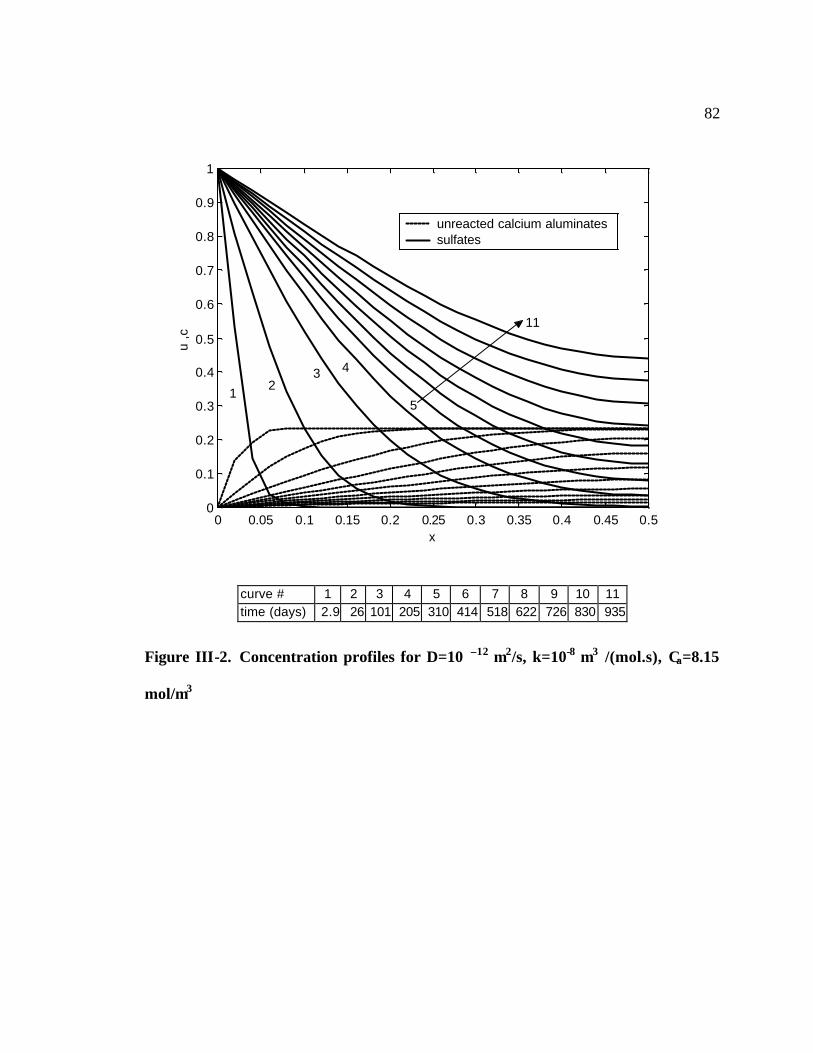
82

curve # 1 2 3 4 5 6 7 8 9 10 11 time (days) 2.9 26 101 205 310 414 518 622 726 830 935

Figure III-2. Concentration profiles for D=10 –12 m2/s, k=10-8 m3 /(mol.s), Ca=8.15

mol/m3

0 0.05 0.1 0.15 0.2 0.25 0.3 0.35 0.4 0.45 0.50

0.1

0.2

0.3

0.4

0.5

0.6

0.7

0.8

0.9

1u

,c

x

unreacted calcium aluminatessulfates

1 2

3 4

5

11

83

curve # 1 2 3 4 5 6 7 8 9 10 11 time (days) 5.8 52 214 434 654 874 1094 1314 1534 1754 1973

Figure III-3. Concentration profiles for D=10 –12 m2/s, k=10-8 m3 /(mol.s), Ca=8.15

mol/m3

0 0.05 0.1 0.15 0.2 0.25 0.3 0.35 0.4 0.45 0.50

0.5

1

1.5

2

2.5

u ,c

x

unreacted calcium aluminatessulfates

1 2 3

4 5 to 11

84

curve # 1 2 3 4 5 6 7 8 9 10 11 time (days) 11.6 104 289 590 891 1192 1493 1794 2095 2396 2697

Figure III-4. Concentration profiles for D=10–12 m2/s, k=10-8 m3 /(mol.s), Ca=252

mol/m3

Then the influence of the value of the rate constant k on the evolution of the

calcium aluminates concentration profiles is presented in, Figure III-5, Figure III-6 and

Figure III-8. As expected, when the rate constant increases, so does the rate of

consumption of calcium aluminates. But it can be seen that the influence of the rate

0 0.05 0.1 0.15 0.2 0.25 0.3 0.35 0.4 0.45 0.50

1

2

3

4

5

6

7

8

u ,c

x

unreacted calcium aluminatessulfates

1 2

3

4 5 to 11

85

constant value is important only for the lowest calcium aluminates initial content. In this

case, as time increases, the difference between the various curves diminishes. The

anomalies observed for Ca =8.15 mol/m3 and k=10 –6 m3 /(mol.s) are not being explained.

Figure III-5. Influence of rate constant on “CA” profiles for Ca =8.15 mol/m3

0 0.05 0.1 0.15 0.2 0.25 0.3 0.35 0.4 0.45 0.50

0.05

0.1

0.15

0.2

0.25

c

x

k=10-6

10-7

10-8

10-9

20 days

135 days

550 days

86

Figure III-6. Influence of rate constant on “CA” profiles for Ca =82.5 mol/m3

0 0.05 0.1 0.15 0.2 0.25 0.3 0.35 0.4 0.45 0.50

0.5

1

1.5

2

2.5

c

x

k=10-6

10-7

10-8

10-9

20 days

450 days

920 days

1730 days

87

Figure III-7. Influence of rate constant on “CA” profiles for Ca =252 mol/m3

The effect of increasing the value of the diffusivity is to increase the time to

completion of the reaction, i.e. the time necessary to consume all the initially present

calcium aluminates. This is shown in Figure III-8. The effect of a 10-fold increase of D is

much more important than the same operation on the rate constant.

0 0.05 0.1 0.15 0.2 0.25 0.3 0.35 0.4 0.45 0.50

1

2

3

4

5

6

7

8c

x

k=10-6

10-7

10-8

10-9300 days

600 days

70 days

1210 days

2440 days

88

Figure III-8. Effect of diffusivity on the end of reaction time for different rate

constants and initial calcium aluminate contents

0 50 100 150 200 250 30010

1

102

103

104

105

initial calcium aluminate content (mol/m3 of mortar)

time

to c

ompl

etio

n of

rea

ctio

n (d

ays) D=10-13 m2/s

D=10-12 m2/s

D=10-11 m2/s

k=10-7 mol/m3/s

k=10-8 mol/m3/s

k=10-9 mol/m3/s

89

3.5.2.5. Effect of cracking

As pointed out by several authors, expansion due to ettringite formation leads to

cracking, hence to an increase of the diffusion coefficient. Likewise, softening due to the

chemical action of sulfates on calcium hydrates, tends to increase the diffusion

coefficient. This change in the diffusion coefficient is probably not defined by a

rigorously defined sharp boundary. In a first approach, it is proposed that the material

subjected to sulfate attack be divided into two regions, one comprised between the

surface and a plane of abscissa XS with a diffusion coefficient D1, and a region comprised

between X=XS and X=L/2 (plane of symmetry), with a diffusion coefficient D2 lower

than D1 (discontinuous diffusivity). D2 represents the diffusion coefficient of the original

unaltered material. The boundary moves with time towards the middle of the slab. The

rate of motion is imposed by the value of the total amount of calcium aluminate that has

reacted, provoking the initiation of cracks.

The geometry of the problem is presented in Figure III-9.

90

(a)

(b)

Figure III-9. Geometry of moving boundary problem, with discontinuous

diffusivity. (a) at T=0. (b) at T>0

D2

X

plane of symmetry

L/2

D

XS (0)=0

D2

D1

0 X

plane of symmetry

L/2

D

XS (T)

uncracked zone cracked zone

91

Then, in a second approach, the diffusivity D1 in the cracked zone will be

considered as a variable of the damage due to cracking. The damage parameter takes a

value between 0 (when the material is undamaged), and 1 (when it has failed) and will be

defined further in detail in the subsequent sections. This leads to a case of continuous

diffusivity. A linear relationship between damage parameter ω and diffusivity D will be

assumed (see also Figure III-10):

( ) ( ) 221 DDDD +−= ωω

Figure III-10. Schematic representation of the assumed relationship between

diffusivity and damage parameter

ω10

D2

D1

D

92

Since the damage parameter is not likely to be a linear function of the abscissa X,

the variation of D with X is not likely to be linear, either (see Figure III-11).

Figure III-11. Geometry of moving boundary problem, with continuous diffusivity,

at T>0

For the present work, a maximum increase of the diffusivity by a factor of 10, as

suggested in the literature206, has been chosen. That is: ( )

102

max1 =D

D for ω =1.

3.5.2.6. Numerical solution of the moving boundary diffusion-reaction equation

The methodology to solve the moving boundary diffusion-reaction equation is the

following:

1. solve the equation for the fixed boundary (composite medium).

D2

D1

0 X

plane of symmetry

L/2

D

XS (T)

93

2. solve the moving boundary problem for the diffusion equation with no reaction

(second Fick’s law with moving boundary), for the two cases: discontinuous and

continuous diffusivity.

3. apply the method devised for the previous step to the moving boundary diffusion-

reaction equation.

The solution for the first step (composite medium), based on the notion of

“junction conditions” 207,208 and using a method of fictitious values209, is described in

Appendix C.

The moving boundary problem for the diffusion equation is solved numerically

assuming we are in the case of a discontinuity of the diffusion coefficient at a given

concentration210. Moving boundary problems, also referred as Stefan problems 211

constitute a subset of diffusion problems. Although analytical methods are available for

some cases, very often numerical methods are necessary212. The numerical solution for

the second step of the methodology described above is reported in Appendix E. This

solution is based on a method developed for a problem of oxygen diffusing in an

absorbing tissue 213,214,215. The expression of the analogs of the space derivatives for

uneven space intervals 216 will be required. In the case of discontinuous diffusivity only, it

will be possible to compare the results with an analytical solution217.

The third step is the combination of the methods developed for the diffusion-

reaction equation without a moving boundary and the diffusion problem with a moving

94

boundary but no reaction. The mathematics involved in this step is presented in Appendix

G. The criterion for boundary motion is based on the concentration of reacted “CA”:

when a conventional value of reacted C3A is detected at a point, it is decided that the

material between this point and the surface, is cracked, thus displays a higher diffusivity.

As for the model without cracking, the computation are stopped when all the “CA” is

consumed.

3.5.2.7. Crystallization pressure of ettringite

Expansion due to ettringite formation results in build-up of internal pressure.

Thermodynamical considerations have been developed to calculate the so-called

crystallization pressure P. It has been pointed that the proposed equations are of the form:

LnAVRTP

s

= , the term A has been defined differently by various authors218.

Based on Riecke principle, the following equation has been derived for the

crystallization pressure of a salt219:

=

ss CCLn

VRTP

with R as the ideal gas constant, T temperature, Vs molar volume, C actual

concentration of the solute during concentration, and Cs saturation concentration. For

ettringite, with a molar weight of 1252 g and a specific gravity of 1.78 g/cm3, P ranges

95

from 2.4 to 8.1 MPa for a degree of supersaturation C/Cs of 2 to 10, at a temperature of

25°C.

Using Gibb’s free energy, another equation has been proposed220,221 :

=−=

0

0

sp

sp

s

ss KK

LnVRT

PPP

with spK the solubility product of the crystallite under pressure sP , 0spK the

solubility product of the crystallite under pressure 0sP (atmospheric pressure). The value

of 0spK at 25°C for ettringite vary from 10-43.13 (reference222) to 10-44.91 (reference 223).

Other values can be found in the literature224. According to the authors of reference 220,

0spK is so low that the condition 0

spsp KK > “can be readily met for practical […] cement

paste/sulphate solution systems”, which implies that P>0. For ratios of 0sp

sp

K

Kidentical to

degrees of supersaturation C/Cs of 2 to 10, at a temperature of 25°C, the same

crystallization pressures are obtained. Although no data for spK at higher pressure is

available, one can consider that, even for high 0sp

sp

K

Kratios, crystallization pressures of the

same order of magnitude can be reached, due to the decreasing slope of the logarithm

function. Data for spK as a function of temperature225 indicate that at a temperature of

96

70°C (temperature at which ettringite begins to thermally degrade), the ratio0sp

sp

K

Kis equal

to 10.8, which would correspond to a pressure of 9.7 MPa.

By taking into account the “change of interface energy”, the crystallization

pressure of ettringite at 25°C was found equal to 55.5 MPa for portland cement 226.

Another approach is based on the ratio of the solubility products of the solid

reactants and product, as expression for the term A. From the reaction of formation of

ettringite from SAC 34 , lime and gypsum, a value of 71 MPa has been computed for the

crystallization pressure227.

Damaging effects of crystal growth pressure on brittle materials have been

illustrated experimentally228.

3.5.2.8. Effect of crystallization pressure of ettringite

Expansion and cracking in case of internal ettringite formation is believed to be

possible due to stress concentration at the tip of pre-existing cracks229. Even though this

was studied for the case of delayed ettringite formation, it was demonstrated from

thermodynamical considerations that nucleation of ettringite crystals will preferentially

occur in the crack tip 230,231,232 .

It has been shown that when crystallization occur in pores at a distance

comparable to the size of a pre-existing crack, and if the crystallization pressure is high

97

enough, this crack can propagate. The higher the pressure, the smaller the size of a crack

that is able to propagate233.

From linear elastic fracture mechanics, it is possible to compute the stress

intensity factor KI (mode I state) due to the existence of a crack of size c subjected to a

surface load p, placed in a large body234 (see Figure III-12):

cpK I ππ2=

Figure III-12. Schematic representation of a crack in an infinite medium, subjected

to a surface load

p

c

98

For a mortar with a classical value for KIc of = 0.5 MPa. m½ , the critical size of

the crack would be 2 mm for p=10 MPa but only 64 µm for p=55.5 MPa. Even though

the crystallization pressure P is not necessarily uniform, this rough estimation of the

critical size shows that small cracks can propagate under reasonable values of p.

3.5.2.9. Modeling of expansion

The stress due to expansion of ettringite will be modelled using the

micromechanical description of the response of concrete to uniaxial tension235. The

typical stress-strain curve is composed of several sections responsible for various

mechanisms, the peak corresponding to the ultimate stress ft , and is divided into three

region (see Figure III-13):

q A linear elastic response (from O to A), characterized by a deformation

modulus E0. In this region, the material is considered as undamaged (ω=0).

q A pre-peak region (from A to B), where microcracks are initiated then grow,

which leads to a linear decrease of the modulus E with increase of the damage

parameter (E<E0).

q A post-peak region (from B to C), where microcracks continue to propagate

up to failure of the specimen. This region is affected by the amount of damage

reached at the peak.

99

Figure III-13. Schematic representation of the tensile stress-strain response of

concrete

Pre-peak region model.

The damage parameter is related to a parameter called crack density Cd (number

of cracks per unit volume), by the relation: dC9

16≈ω . The crack density has been

empirically correlated to the strain at any level between A and B: ε, and the so-called

threshold strain ε th, that corresponds to point A (initiation of cracks):

3.2)1(16.0ε

ε thdC −×= .

ω0

0

×

O strain εth εp C

A

B

stress damage (ω)

×

×

× 1

ω

×

100

This expression of Cd is used in the relation dC9

16≈ω , which enables one to

calculate E for each strain level ε, using the relation: E=E0(1-ω). This relation expresses

the reduction of stiffness due to increase of damage.

Post-peak region model (Horii et al. model.).

In this model, the value of the stress is obtained from the damage parameter with

the relation:

)2/tan()2/tan(

'0

πωπωσ

=tf

, where ω0 is the damage accumulated at the peak. The value of ω0

is obtained from the strain at peak using the pre-peak response model. Then, the post

peak deformation w is calculated from the relation:

1)2/log(sec)2/log(sec

' 00

−

=

πωπωσ

tfww

where w0 is the deformation at peak, being equal to: Hw p ×= ε0 , where H is the gauge

length of the specimen, and εp strain at peak.

To each level of the applied strain due to ettringite formation, corresponds a point

on the response curve, which enables to compute the deformation modulus:

q E=E0 in the linear part,

q E=E0(1-ω) in the pre-peak region,

101

q

0εεσ−

=E in the post-peak region, with:

0

0 Ef t

p −= εε . A very low value of E is adopted when the applied strain

exceeds the maximum strain allowed by the model.

Finally, the expans ion of the specimen is obtained through the formula:

−=

0.

11EE

eave

rσ ,

where σr is the residual stress in the specimen due to past history before

sulfate attack (shrinkage), that will be taken here as 2 MPa,

Eave the average modulus over the cross-section (detailed in a subsequent

section).

The applied linear strain is obtained from the volumetric strain εv due to

ettringite formation. Assuming isotropy: 3

vεε = .

The volumetric strain is derived from the volume changes occurring during

conversion of calcium aluminates to ettringite.

For a given reaction:

102

ettringiteSaP →+ , with P any of the three calcium aluminates that

can react, and a the stoechiometric coefficient (2 or 3),

the volume change

∆

P

P

VV

is given by the relationship:

11

1

−+

=

∆

gypsumvPv

ettringitev

P

P

ma

m

m

VV

, with Md

mv = ,

where d, M, and mv are respectively the density, the molar mass and the molar

volume of a given compound. The values of d (from 82) and mv are reported in Table

III-1.

Table III-1. Values of density and molar volume for the different compounds

involved in the chemical reactions

Compound d (g/cm3) mv (kmol./ cm3)

C3A 3.03 11.31

monosulfate 1.95 3.15

C4AH13 2.02 3.62

gypsum 2.32 13.49

ettringite 1.78 1.42

103

The values of

∆

P

P

VV

for the reactions involved are reported in Table III-2.

Table III-2. Values of the volume change for each reaction involved in the sulfate

attack

Reaction

∆

P

P

VV

Monosulfate to ettringite 0.51

C3A to ettringite 1.26

C4AH13 to ettringite 0.48

Because each reactant P is diluted in the concrete, the effect of its intrinsic

expansion is proportional to its concentration. The unit concrete volume change due to P

is:

∑

∆=

∆

PP

P

P

P

P

P

Ptodue cc

dM

VV

VV

,

where the term ∑

PP

P

cc

represents the relative initial molar concentration of a

compound P with respect to the total initial molar concentration of the calcium

aluminates involved, and cP the initial molar concentration of P with respect to the

104

volume of concrete. The method to compute an estimate of the values of cP is given in

Appendix I.

Finally the volumetric strain is obtained through:

∑

∆

=P P

reactedV VV

CAε , where the term CAreacted corresponds to the

concentration of lumped calcium aluminates that has reacted, and is given at any time

and space values by: CA reacted = Ca – C, C being obtained by solving the system of

differential equations. It is noted that the term ∑

∆

P PVV

is a constant for a given

mix design at a given degree of hydration.

Because the ettringite may first fill a fraction of the capillary porosity before

creating a volume change in the concrete, the volumetric strain is reduced by the

corresponding amount:

Φ−= fVcorrectedV εε ,

f being the fraction of capillary porosity being filled, and Φ the capillary

porosity, estimated by236:

+

−=Φ 0,

32.0

39.0max

cw

DRcw

f c ,

105

with cw

being the water/cement ratio, fc the volumetric fraction of cement in the

concrete and DR the degree of hydration of the cement. Obviously, when Φ=0, the

parameter f is not relevant.

Modeling of the moving boundary motion is implemented as the location

where the amount of racted calcium aluminates induces a linear strain that is greater

than the cracking initiation strain(ε th).

3.5.2.10. Adaptation of the 1D solution to a 2D problem

So far, only the case of an infinite slab, i.e. a case of a 1D problem, has been

treated. This case may be present in the field, but no experimental data exist to be

compared to the model. On the contrary, laboratory tests are usually carried on slender

prismatic specimens. Thus it is necessary to adapt the 1D solution to a 2D case.

Diffusion is analog to heat conduction in a medium, and obeys to the same laws.

It has been demonstrated that it is possible to solve a multi-dimensional heat diffusion

problem by the superposition of the solutions of unidimensional cases237. In the present

case, the prism of square cross-section and infinite length (2-D problem) is obtained as

the intersection at right angle of two infinite slabs (2-D problem) of same thickness and

physical properties238 (see Figure III-14).

106

Figure III-14. Application of superposition method to solve case of a prism

When the problem is set up in a dimensionless form, the variable U (temperature

or concentration) is replaced by the va riable Θ such as:

iUUUU

−−

=Θ 0 , with

U0 value of U at the boundary, and

Infinite slabs

Infinite prism

1

2

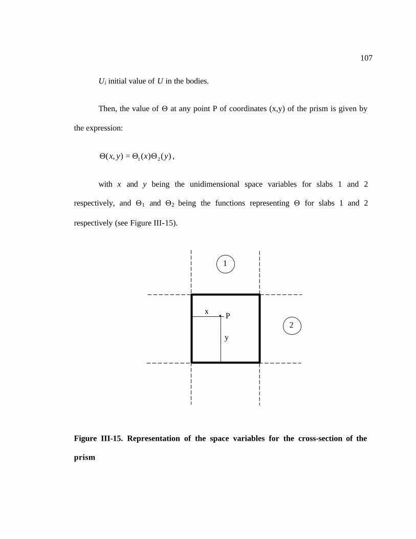
107

Ui initial value of U in the bodies.

Then, the value of Θ at any point P of coordinates (x,y) of the prism is given by

the expression:

)()(),( 21 yxyx ΘΘ=Θ ,

with x and y being the unidimensional space variables for slabs 1 and 2

respectively, and Θ1 and Θ2 being the functions representing Θ for slabs 1 and 2

respectively (see Figure III-15).

Figure III-15. Representation of the space variables for the cross-section of the

prism

× P x

y

1

2

108

Since the sides of the prism are subjected to the same value U0 and Ui we have:

Θ1 = Θ2.

Since the cross-section of the prism is square, and the boundary conditions are

identical over each of its sides, it is sufficient to study the problem over only 1/8 of the

section, the results for the other regions being obtained by translation and/or rotation (see

Figure III-16).

Figure III-16. Illustration of the multiple symmetry of a square cross-section

subjected to identical boundary conditions over each of its sides. The contour line

represented is made up of 8 identical segments.

Region to be

studied

Contour line

109

Finally, when the values of Θ for all couple (x,y) have been computed, the values

of U can be deduced (note: in the present case, Ui=0 for the sulfate concentration).

In the more complex present case of the moving boundary diffusion-reaction

equation, the rigorous proof of the applicability of this superposition method is not

established. As an approximation, the following steps will be applied:

1. the 2D values for the variables U (sulfate concentration) and Z = U –qC are

computed using the superposition method.

2. from these values, the 2D values for C are obtained: q

Z-U C = .

The value of C is then used to compute the value of strain ε. To obtain the strain

over the prism, its cross-section is divided into onion-like concentric layers of thickness

∆X, the innermost layer being a square (see Figure III-17).

110

Figure III-17. Decomposition of the prism cross-section into concentric layers of

constant width

The average strain for each layer is obtained in two steps:

1. Compute the average for the outer and inner perimeters. In order not to

duplicate the weight of the points at the corner and at the middle of the sides,

the following formula for a given perimeter is used:

( )1

21

1

+

++=

∑=

n

n

kkBA

perimeter

εεεε

∆X

∆X

× × × × × × × × × × ×

× ×

× ×

× ×

× ×

× × × × × × × × × × × × × × ×

× × × × × × × × × × ×

× × × × × × ×

× × ×

× : point where U is

computed

“A” points “B” points

concentric

layers

perimeters

111

Where A and B are the points respectively at the corner and at the middle,

n is the number of points between A and B (n=[N+2, N+1…1]),

and εk the values taken by ε at the points between A and N.

For the last perimeter (n=0), which is equal to a single point (center of the

section), the average is simply equal to the value taken by ε at the point.

2. The average for each layer is computed as the average of two consecutive perimeters,

taking in account that the innermost perimeter of each layer possesses 8 less points :

12)1(

+++

=n

nn iolayer

εεε ,

where n is the number of points between A and B for the outermost perimeter,

ε0 the average value for the outermost perimeter,

ε i the average value for the innermost perimeter.

For the last layer (inner square): 9

8 iolayerlast

εεε

+=

with ε0 average value for the last “true” perimeter

and ε i the value of ε at the center.

112

Finally, the average modulus over the entire section is obtained through the

weighted average of all layers, taking into account the area Ai of each layer obtained by

the formula:

)12(4 2 −= idXAi with i=1,2…N+1.

3.6. Validation of model

3.6.1. Diffusivity

The value of the diffusivity of sulfates in cement-based materials is the most

important physical property with respect to resistance to sulfate attack.

If the diffusivity of a given ion in pure water is given as Df, the diffusivity of the

same ion Dp when the water in contained in the pores of a material is:

2τδ

fp DD = ,

where δ is the constrictivity, which defines the non-uniformity of the cross-

section of the pores, and τ the tortuosity, which is linked to the fact that the path direction

imposed by the pores is not necessarily parallel to the concentration gradient. The value

of Df for sulfate ions in water at 25°C is 1.07 × 10-9 m2/s239.

Then, since it is more convenient to consider the flow per unit area of the

material, rather than of the water, the “intrinsic diffusivity” Di is introduced:

113

pi DD ε= ,

where ε is the value of the porosity240.

The value that is actually measured by fitting experimental data to Fick’s law is

the “effective diffusivity” Deff 241. Contrary to chloride ions, values of diffusivity of

sulfate in concrete are scarce in the literature. For a paste with a water/cement ratio of

0.30, values of effective diffusivity at different times of curing, which influences pore

size distribution, range from 4.8 × 10-12 m2/s at 60 days to 1.9 × 10-12 m2/s at 180 days171.

At a higher water/cement ratio (0.40), lower values of diffusivity of pastes are

reported: 0.6 × 10-14 m2/s to 1.34 × 10-14 m2/s at 28 days of exposure115. This is in

apparent contradiction with the values of the pastes previously mentioned.

For a concrete with a water/cement ratio of 0.42, cured at 100%RH for 14 days,

the effective sulfate diffusivity was found variable with the time of exposure to the

sulfate solution, according roughly to the empirical expression242:

76.0710217.2 −− ××= tDeff , with t being the time of exposure in months and

Deff the effective sulfate diffusivity in cm2 /s. Experimental values range from 4.73 × 10-12

m2/s at 16 months to1.06 × 10-12 m2/s at 5 years.

Using radioactive tracers, the diffusivity in mortars was measured equal to 2.7 ×

10-14 to 9.5 × 10-14 m2/s 243. No notable difference between Type I and Type V cements

114

was detected, which is not surprising since the beneficial role of Type V cement is due to

its intrinsic chemistry. Measured diffusivities decrease as a function of time of exposure,

with a two-fold decrease between 4 and 12 weeks, and a much smaller decrease between

12 and 24 weeks. Tests performed on pastes yielded lower diffusion coefficients.

Based on data obtained through EDXA analyses244, diffusivity in concrete with

water/cement ratios from 0.35 to 0.60, and blended or neat binders, was calculated173.

Values range from 1.3 × 10-13 m2/s for a concrete with type I cement and a w/c ratio of

0.50, to 1.7 × 10-15 m2/s for a concrete with slag cement and a w/c ratio of 0.42.

Widely different experimental conditions and methods, as well as the very limited

number of reported values make it difficult to choose a reasonable value for the

diffusivity. It should be emphasized that reactions between ingressing sulfates and

cement paste profoundly alter the diffusion process, thus the effective diffusivity is likely

to be very different from the intrinsic diffusivity 245.

The following values of the intrinsic sulfate diffusivity for concrete have been

reported174: 1.05 × 10-11 m2/s for w/c = 0.45 and 3.54 × 10-11 m2/s for w/c = 0.65. Also,

taking into account the effect of sulfate attack on the value of the porosity of the cement

paste, these authors have estimated that the diffusivity of a paste can be increased by a

factor of up to10.

115

Attempts have been made to relate intrinsic ion diffusivity D and water

permeability coefficient K. The relation: b

f

D D8A K

2π= , has been proposed, where A is

the cross-sectional area and b a constant suggested to be taken as 1.5 246. When this

relationship is applied to both chloride and sulfate ions, K and A being identical, one

obtains:

b

Clf

SOfClSO D

DDD

2

4

4

= . From this expression, it is possible to calculate

4SOD if

DCl is known, the value of Df Cl at 25 °C being equal to 2.03 × 10-9 m2/s 239. For example,

with chloride diffusivity of regular strength concrete and mortar ranging from 1× 10-12 to

10 × 10-12 m2/s 247,248 , corresponding values for sulfates would be 2× 10-12 to 20 × 10-12

m2/s. It is noted that some authors presenting models for sulfate attack161,173,177,178 have

chosen diffusivities comprised between 0.75 ×10-12 and 9 ×10-12 m2/s, often with no

specific justification.

3.6.2. Mortar tests

Majority of the mortar tests are based on ASTM standard C 1012. Various

modifications may be introduced by several authors. Among these modifications, the

process which controls the pH of the solution appears to be very important. The standard

test requires that the external sulfate concentration be constant, but does not take into

account the modification of the sulfate solution that occurs when the volume of solution

116

is not very large compared to the volume of the specimen. What is observed in that case

is a shift in the pH of the solution due to outward migration of OH- ions from the cement

paste, due to the sulfate attack. In the field, the volume of surrounding solution is much

more important than the element of structure, and constantly renewed, which prevents the

pH shift. Consequently, it has been proposed that the pH of the solution be monitored

during the test and adjusted to a constant value by acidic addition249,250. Circulation of the

solution around the sample with a pump has also been implemented.

Keeping the pH constant was shown to accelerate the test, from the loss of

strength as well as from the expansion viewpoint. Comparative tests between pH-

controlled and pH-non controlled conditions show that the time to reach a certain level of

expansion for the pH-non controlled condition is roughly twice as much as for the pH-

controlled condition251,252. Since the migration of OH- ions is not accounted for in the

present model, expansion results from pH-non controlled tests will be converted to

equivalent pH-controlled test data, by dividing the time scale by a factor of two.

The ASTM C1012 standard prismatic mortar bar have a cross-section 25 × 25 mm

and a gage length of 250 mm. The standard w/c ratio is 0.485.

The rate constant of reaction has been taken equal to 10-7 m3/mol.s. No data were

readily available from the literature.

117

The concentration of the standard solution surrounding the mortar bar is 352

mmol. of sulfates/l of solution. For a classical value of porosity of 10% for a mortar, this

concentration is equivalent to 35.2 mol/m3 of mortar.

The solution used is sodium sulfate for all tests, except tests reported in 254 and 255

(mix of magnesium sulfate and sodium sulfate).

The program is executed until the maximum time of the experiment, or

exhaustion of calcium aluminates. The initial number of space intervals is 25. The Matlab

program was run in a UNIX environment (HP 700 and Sun Solaris 7 platforms).

3.6.2.1. Tests by Lagerblad253

The tests conducted were pH-controlled. Two cements were used, an ordinary

portland cement (OPC) and a sulfate resistant portland cement (SRPC) with respectively

7.7% and 1.2% of C3A. Mortars were prepared with the standard water/cement ratio of

0.485 and a w/c ratio of 0.32 for the OPC only.

The parameters used to predict the expansion vs. time with the model are reported

in Table III-3. The results are shown in Figure III-18 and Figure III-19.

118

Table III-3. Parameters used to fit experimental data (Lagerblad – mortars)

D2 (m2/s) f ft (MPa) E0 (GPa)

OPC w/c=0.485 5 ×10-13 0.3 4.5 20

OPC w/c=0.32 2 ×10-14 NR 7 25

SRPC w/c=0.485 5 ×10-13 0.05 4.5 20

NR: not relevant.

Figure III-18. Validation of model for data by Lagerblad (mortars – OPC)

0 50 100 150 200 250 300 350 4000

0.5

1

1.5

2

2.5

3

3.5

4

4.5

5x 10

-3

time (days)

linea

r ex

pans

ion

experiment w/c=0.485model experiment w/c=0.32

119

Figure III-19. Validation of model for data by Lagerblad (mortar – SRPC)

It is noted that both mortars with w/c=0.485 were assigned comparable diffusivity

and mechanical properties, and the OPC mortar with a lower w/c ratio, a lower diffusivity

and higher strength. Also the parameter f is much less for SRPC than OPC.

3.6.2.2. Tests by Ferraris et al.. 252

These tests were also pH-controlled. The C3A content of the cement was high at

12.8%. the w/c ratio used was standard. The value of the parameters for fitting the data

are reported in Table III-4. The results are shown in Figure III-20.

0 50 100 150 200 250 300 350 4000

0.5

1

1.5

2

2.5

3

3.5

4

4.5

5x 10

-3

time (days)

linea

r ex

pans

ion experiment

model

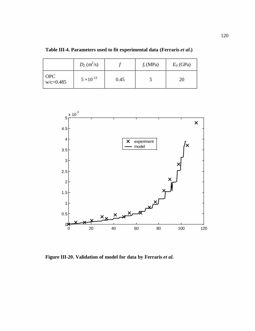
120

Table III-4. Parameters used to fit experimental data (Ferraris et al.)

D2 (m2/s) f ft (MPa) E0 (GPa)

OPC w/c=0.485 5 ×10-13 0.45 5 20

Figure III-20. Validation of model for data by Ferraris et al.

0 20 40 60 80 100 1200

0.5

1

1.5

2

2.5

3

3.5

4

4.5

5x 10

-3

experimentmodel

121

Since the mix design parameters are the same as for the previous example,

comparable values of physical and mechanical characteristics have been introduced.

3.6.2.3. Tests by Brown 251

These tests are also pH-controlled, but the w/c ratio is chosen as 0.60, with a

cement at 14% C3A. The value of the parameters for fitting the data are placed in Table

III-5 The results are shown in Figure III-21.

Table III-5. Parameters used to fit experimental data (Brown)

D2 (m2/s) f ft (MPa) E0 (GPa)

OPC w/c=0.60 5 ×10-12 0.6 4 18

122

Figure III-21. Validation of model for data by Brown

It is noted that the choice of physical and mechanical properties reflects the higher

value of the w/c ratio, compared to the standard test.

3.6.2.4. Tests by Ouyang et al. 254

These tests were not pH-controlled but are interesting because four cements with

increasing C3A content are being used. Thus the time scale was divided by two for the

experimental data. The parameters retained to compare the experimental data to the

predicted values are reported in Table III-6. The results are shown in Figure III-22 and

Figure III-23.

0 10 20 30 40 50 600

1

2

3

4

5

6

7

8x 10

-3

time (days)

expa

nsio

n

experimentmodel

123

Table III-6. Parameters used to fit experimental data (Ouyang et al.)

C3A content (%) D2 (m2/s) f ft (MPa) E0 (GPa)

4.3 8 ×10-13 0.25 5 20

7.0 7 ×10-13 0.30 5 20

8.8 7 ×10-13 0.30 5 20

12 7 ×10-13 0.35 5 20

Figure III-22. Validation of model for data by Ouyang et al.

0 20 40 60 80 100 120 140 160 1800

0.5

1

1.5

2

2.5

3

3.5

4

4.5

5x 10

-3

time (days)

linea

r ex

pans

ion

C3A=4.3 %model C3A=8.8 %

124

Figure III-23. Validation of model for data by Ouyang et al

Practically, all physical and mechanical parameters are identical, because the

same mix design was used.

3.6.2.5. Tests by Mobasher and Ariño 255

These tests were not pH-controlled, but they compare mix designs with and

without copper slag, for two water/cement ratios: 0.40 and 0.50. For the water/cement

ratio of 0.50, no difference was noted between mortars with or without slag, meaning

that, for this w/c ratio, the presence of slag did not modify significantly the physico-

chemical properties. Hence, only the mortars with a w/c ratio of 0.40 will be compared.

0 20 40 60 80 100 120 140 1600

0.5

1

1.5

2

2.5

3

3.5

4

4.5

5x 10

-3

time (days)

linea

r ex

pans

ion

C3A= 7 % C3A= 12 %model

125

Because the authors do not indicate the chemical composition of the cement, but only its

type (ASTM Type I), classical values of 7% and 6% for respectively the C3A and gypsum

content have been retained.

The parameters corresponding to model fitting trials are reported in Table III-7.

The results are shown in Figure III-24.

Table III.7- Parameters used to fit experimental data (Mobasher and Ariño)

binder nature D2 (m2/s) f ft (MPa) E0 (GPa)

100% OPC 6 ×10-13 0.4 5.5 22

90% OPC –10% copper slag 4 ×10-13 0.4 5.5 22

126

Figure III-24. Validation of model for data by Mobasher and Ariño

3.6.3. Concrete tests

The solution used is sodium sulfate for all the tests.

3.6.3.1. Tests by Lagerblad253

These tests were conducted on 75 × 75 × 300 mm prisms, and pH-controlled, with

the same cements as for the mortar study, and three different w/c ratio: 0.55, 0.45 and

0.35. It should be noted that these prisms are less slender than their mortar counterparts.

Also, while they were standing upright in the solution, their uppermost part was left

0 20 40 60 80 100 120 1400

0.5

1

1.5

2

2.5

3

3.5

4

4.5x 10

-3

100 % OPC model 90 % OPC 10 % slag

127

above the surface, to enhance the penetration of sulfates ions. This particular boundary

condition is not taken into account in the model. The values chosen for the parameters

used to fit the model are displayed in Table III-8. The results are shown in Figure III-25,

Figure III-26 , Figure III-27 and Figure III-28.

Table III-8. Parameters used to fit experimental data (Lagerblad – concrete)

cement type w/c ratio D2 (m2/s) f ft (MPa) E0 (GPa)

0.55 1 ×10-12 0.35 3 20

0.45 5 ×10-13 0.45 4 22

OPC

0.35 6 ×10-14 NR 6 25

0.55 8 ×10-13 0.05 3 20

0.45 5 ×10-13 0.05 4 22

SRPC

0.35 1 ×10-13 NR 5 24

128

Figure III-25. Validation of model for data by Lagerblad (concrete – OPC)

0 200 400 600 800 1000 1200 1400 1600 18000

0.5

1

1.5

2

2.5x 10

-3

time (days)

linea

r ex

pans

ion

w/c=0.55 model w/c=0.45 w/c=0.35

w/c=0.45

w/c=0.35

w/c=0.55

129

Figure III-26. Validation of model for data by Lagerblad (concrete – SRPC,

w/c=0.55)

0 200 400 600 800 1000 1200 1400 1600 18000

0.5

1

1.5

2

2.5x 10

-3

time (days)

linea

r ex

pans

ion

experimentmodel

130

Figure III-27. Validation of model for data by Lagerblad (concrete – SRPC,

w/c=0.45)

0 200 400 600 800 1000 1200 1400 1600 18000

0.5

1

1.5

2

2.5x 10

-3

time (days)

linea

r ex

pans

ion

experimentmodel

131

Figure III-28. Validation of model for data by Lagerblad (concrete – SRPC,

w/c=0.35)

3.6.3.2. Tests by Von Fay256

These tests were run on 76.2 × 152.4 mm cylinders, without control of the pH.

Since the ratio height/diameter of the specimen is only 2, the ingress of sulfates through

the ends could not be ignored, compared to that of through the lateral surface. As an

approximation, it was assumed that this accelerating effect was equal in magnitude to the

fact that the test is not pH-controlled, which is a retarding effect.

0 200 400 600 800 1000 1200 1400 1600 18000

0.5

1

1.5

2

2.5x 10

-3

time (days)

linea

r ex

pans

ion

experimentmodel

132

The shape of the cross-section, square or circular, has an influence on the

diffusion process. Comparative tests on 25 mm diameter cylinders and 25 × 25 mm

prisms have shown no difference from the expansion viewpoint252. Also, it is possible to

show, using only Fick’s law, that the quantity of ions having ingressed in a cylinder after

a short amount of time is comparable to that in a prism of same cross-section area (see

Appendix J). Thus, trials were run on an equivalent prism of 67.5 mm side.

The C3A content of the cement is 4.6% and the w/c ratio 0.36. The parameters

retained are shown in Table III-9. The results are shown in Figure III-29.

Table III-9. Parameters used to fit experimental data (Von Fay)

D2 (m2/s) f ft (MPa) E0 (GPa)

1 ×10-13 0.5 6 25

133

Figure III-29. Validation of model for data by Von Fay

3.6.4. Discussion

The choice of the values for D2 (undamaged material diffusivity) is consistent

with the water/cement ratio of the mix designs, as well as the choice of the values for the

mechanical parameters. When all other parameters are kept the same, lower values of w/c

lead to a lower diffusivity, hence to a slower expansion rate. This is predicted by the

model.

0 200 400 600 800 1000 1200 1400 1600 18000

1

2

3

4

5

6x 10

-4

time (days)

linea

r ex

pans

ion

experimentmodel

134

For a very low C3A content (Lagerblad, mortars and concrete, sulfate resistant

portland cement), the potential expansion predicted by the volume change during

chemical reactions, is very low, which explains why the parameter f had to be chosen

much lower than for OPCs. With higher values, no expansion would be predicted because

the capillary porosity would be higher than the chemical expansion. In reality, it is known

that hydrates from the hydration of C4AF, although not supposed to be potentially

expansive, might still bring some expansion (see 3.4), which is not taken in account in the

model. This is confirmed by the fact that, for the SRPC mortar and the SRPC concrete

with w/c ratios of 0.55 and 0.45, the model predicts that the reaction ends due to

exhaustion of calcium aluminates, before the experimentally measured expansion ceases

to increase.

Size effect is also predicted by the model, since for comparable w/c ratios (0.485

and 0.45 respectively for small mortars prisms and large concrete prisms), the same

diffusivity and comparable f have been used for the prediction.

Differences in the choice of f may be due to:

q the composition of the cement, and not only the content in C4AF, but also in

calcium silicates, that are responsible for the production of calcium hydroxide,

which is also involved in the degradation process and not taken into account

in the model,

135

q the presence of magnesium in the external solution, for two of the mortar

tests.

3.7. Conclusions

The principles behind the mechanisms of sulfate attack of cement-based materials

have been described, with special emphasis on the areas which are not clearly understood

nowadays. Methods to prevent sulfate attack are known through mainly use of low-C3A

cements, design of mixes with low water/cement ratio and introduction of mineral

admixtures such as copper slag in the mix design. The present approach presents a

quantitative method to assess the expansion results with the microstructural features.

The literature presents various types of models, not always compared to

experimental data, nor founded on the same assumptions.

The model presented here is based on both chemistry (rate of reaction, volume

change during reaction), physics (diffusion with moving boundary and variable

diffusivity) and mechanics (stress-strain response of concrete).

The final model is derived successively from the solution of the diffusion-reaction

equation, then the addition of the moving boundary effect, the change of diffusivity due

to cracking, and finally the approximate adaptation of the 1-D solution to the 2-D case of

a square cross-section prism. This model can be used to define acceptable expansion

values and tolerable expansion and damage rates.

136

Experimental data for tests that have not been controlled, had to be empirically

modified to comply with the model which does not take into account any variability in

the environment.

Simulations indicate reasonable agreement with experimental data, when

unknown parameters are chosen in a compatible way with the actual mix design of the

materials. The most important discrepancies are observed for very low C3A, probably due

to the fact that the effect of calcium ferro-aluminate is neglected.

The following improvements to the present model are suggested:

q verification of stability and convergence conditions of the numerical solution.

q introduction of the effect of decalcification, especially when magnesium

sulfate is present, on the diffusion and mechanical properties.

q possibility of choosing other possible mechanisms of expansion due to

ettringite, other than volume change112.

q introduction of more accurate models for the stress-strain response of

concrete.

q utilization of diffusivity models involving the ITZ (interfacial transition zone)

for mortars and concrete257.

q more rigorous establishment of the numerical solution for the 2-D and 3-D

cases.

137

q generalization to the case of surfaces subjected to evaporation under wetting

and drying cycles.

q generalization to the case of internal sulfate attack.

Also, more experimental work should be carried out both on the design of

performance tests and the understanding of the microstructural changes occurring during

external sulfate attack:

q measurement of both physical (expansion, crack density) and mechanical

parameters (strength, modulus, fracture parameters) during a performance test.

q determination of the intrinsic sulfates diffusivity for various mix designs and

binder nature.

q quantification of the role of C4AF in the degradation process, and of the

importance of the C3S/C2S content.

q confirmation of the nature and stoechiometry of the reactions taking place

during sulfate attack.

q determination of the location and the effect of ettringite formation.

CHAPTER 4

CONCLUSION

In this study, the beneficial aspects of blended cements have been emphasized

from the standpoint of concrete durability.

A given mineral admixture, slag from copper metallurgy, was extensively

characterized, and its effects on portland cement hydration examined. From these tests, it

was concluded that the improvements brought by copper slag to blended cement concrete

are likely to be the consequence of a densification of the microstructure. Another research

effort, which will be published in a journal, was aimed towards enhancing the reactivity

of the blend copper slag/ portland cement by mutual grinding in a prototype jet-mill.

Numerous studies have been undertaken worldwide on the topic of blended

cements. During the years 1997 and 1998 only, almost 900 references have been reported

in the area of blended cements. These references were described and categorized in

separate publications 258,259. A lot of these studies addressed the durability problems and

show the enhancement of performance in term of durability due to the presence of

mineral admixtures. Thus, it is possible to use the results of these studies (and those

published in other years) to design durable concrete with different types of blended

cements. Very few of these studies however tried to quantitatively relate the

microstructure to the measures of durability such as expansion, and service life.

In the present study, durability concerns have been focused on the modeling of

external sulfate attack. A literature research has exposed the different theories trying to

139

explain the mechanisms underlying this complex phenomenon. Existing models have

been described, with special emphasis on their diversity. A model has been developed

based on a finite difference analog of the diffusion-reaction equation. To introduce the

effect of cracking due to expansion of the cement matrix, a moving boundary problem

with variable diffusion coefficient was used. After extrapolation of the 1-D solution to the

2-D case, it was possible to validate the outputs of the model by comparing it to

experimental results. Unknown parameters were chosen by taking into account the mix

designs given by the authors of these experiments. It appeared that the C3A content of the

portland cement is the most important mineralogical parameter, and the diffusivity the

most important physical property. One of the issues which still needs to be determined is

the location of formation of ettringite, responsible for the expansion. The through

solution mechanism was used in the present model. In addition the level of filling up of

the capillary porosity needs to be addressed. The most promising directions to continue

this research is obtained by a better understanding of the mechanisms of sulfate attack,

further measurements of the diffusion coefficient, and improvements to the chemical side

of the model.

REFERENCES

1 Mehta, P. Kumar. “Role of pozzolanic and cementitious material in sustainable

development of the concrete industry.” Fly Ash, Silica Fume, Slag, and Natural

Pozzolans in Concrete. Sixth CANMET/ACI/JCI Conference. Ed. V.M. Malhotra.

Detroit: American Concrete Institute, 1998. pp. 1-20.

2 Biswas, A.K. and W.G. Davenport. Extractive metallurgy of copper. Third Edition.

Oxford, England: Elsevier Science, 1994.

3 Newton, Joseph and Curtis L. Wilson. Metallurgy of copper. New York: John Wiley

and Sons, 1942.

4 Moranville-Regourd, Micheline. “Cements made from blastfurnace slag.” Lea’s

Chemistry of cement and concrete. Ed. Peter C. Hewlett. Fourth Edition.. London,

England: Arnold, 1998. 633-674

5 Douglas, E., P. R.Mainwaring and R. T.Hemmings. “Pozzolanic Properties Of Canadian

Non-Ferrous Slags.” Fly Ash, Silica Fume, Slag, and Natural Pozzolans in

Concrete. Proceedings - Second International Conference. Ed. V.M. Malhotra.

Detroit: American Concrete Institute, 1986. v. 2:1525-1550.

6 Wozniak, K. “Cutting property assessment of copper slag grains.” Metal Finishing

86.Nov. 1988 (1988): 37-40.

141

7 Chopra, Manjit S. and Stephen F. Mehlman. “Abrasive formulation for waterjet cutting

and method employing same.” US Patent 5637030 (1997).

8 Shoupeng, Jiang and Zhang Qi. “Method for producing rust removal grinding

compound using copper metallurgy slag.” CN Patent 1196377 (1998).

9 Madany, Ismail M., Mohammad H. Al-Sayed, and E. Raveendran. “Utilization of

copper blasting grit waste as a construction material.” Waste Management 11.1-2

(1991): 35-40.

10 Tayeb, Aghareed-M. “Use of some industrial wastes as energy storage media.” Energy-

Conversion-and-Management 37.Feb.96 : 127-33.

11 Qiang, Sun and Zhang Shuzhen. “High-strength powder coal ash inorganic artificial

marble and making method.” CN Patent 1096281 (1994).

12 Schwenke, Raimar. “Coverings or components (building components) having a brick-

like structure and a process for the production thereof.” DE Patent 3728019

(1989).

13 Nafziger, R. H and J.E. Tress. “Electric Furnace Melting Of By-Product Metallurgical

Slags.” CIM Bulletin 69.772 (1976): 73-78.

14 “Mine filling installations at Mount Isa.” Mining Magazine 130.4 (1974):244-253.

142

15 Kirkby, R. W. and J. V. Happ. “Utilization of waste material as fill in a large scale

mining operation.” Treatment, Recycle and Disposal of Wastes Proceedings of the

Third National chemical engineering conference, Mildura, Victoria, Australia.

Clayton, Australia: Monash University, 1975. T29-T31.

16 Leahy, F.J. and Cowling R. “Stope developments at Mount Isa.” Mining with

Backfilling. Proceedings of the 12th Canadian Rock Mechanics Symposium. May

21-29 1978. Montreal: Canadian Institute of Mining and Metallurgy, 1978. 129-

132.

17 Thomas, E. G. and R.Cowling. “Pozzolanic behaviour of ground Isa mine slag in

cemented hydraulic mine fill at high slag/cement ratios.” Mining with Backfilling.

Proceedings of the 12th Canadian Rock Mechanics Symposium. May 23-25 1978.

Montreal: Canadian Institute of Mining and Metallurgy, 1978. 129-132.

18 Hull, Bruce. “Magma’s sandfill system as employed at the Magma mine, Superior,

Arizona, USA.” Mining with Backfilling. Proceedings of the 12th Canadian Rock

Mechanics Symposium. May 23-25 1978. Montreal: Canadian Institute of Mining

and Metallurgy, 1978. 75-83.

19 McGuire, A.J. “Falconbridge slag as a cementing agent in backfill” Mining with

Backfilling. Proceedings of the 12th Canadian Rock Mechanics Symposium. May

143

23-25 1978. Montreal: Canadian Institute of Mining and Metallurgy, 1978. 133-

138.

20 Yu, T.R. and Counter D.B. “Backfill practice and technology at Kidd Creek Mines.”

CIM Bulletin 76.856 (1983): 56-65.

21 Atkinson, R.J., A.L Hannaford, L.Harris, and T.P Philip. “Using smelter slag in mine

backfill.” Mining Magazine 160.8(1989): 118-123.

22 Ferguson, Robert E. and Braja M. Das. “Use of copper slag for construction purposes.”

Structures Congress Proceedings of the Sessions Related to Structural Materials.

May 1-5 1989, San Francisco. New York: ASCE, 1989: 323-332

23 Hwang, C.L. and J.C. Laiw. “Properties of concrete using copper slag as a substitute of

fine aggregate.” Fly Ash, Silica Fume, Slag, and Natural Pozzolans in Concrete.

Proceedings - Third International Conference. Ed. V.M. Malhotra. Detroit:

American Concrete Institute, 1989. v. 2:1677-1695.

24 Malhotra, V.M. “Fly Ash, Silica Fume, and Rice-Husk Ash in Concrete: a review.”

Concrete International April 1993:23-28 (1993)

25 Krofchak, David.”A method of making cement from base metal smelter slag.” World

Patent 9824732 (1998).

144

26 Krofchak, David. ”Method of making concrete from base metal smelter slag” US

Patent 593493 (1997).

27 Laneuville, J. “Portland cement-slag binders.” CA Patent 963482 (1975).

28 Baragano, J.R. “The study of a non traditional pozzolan: copper slags.” Proceedings of

the 6th International congress on the chemistry of cement .1980: III.37-III.42.

29 Emery, J.J. “Canadian developments in the use of by-products.” CIM Bulletin Dec

.1979: 88-94 (1979).

30 Emery, J.J. “New uses of metallurgical slags.” CIM Bulletin Dec .1975: 60-68 (1975).

31 Collings, R. K. ”Mineral Wastes.” CIM Special Volume 29: 337-341 (1984).

32 Collins, R. J. and S. K. Ciesielski. “Recycling and Use of Waste Materials and

Byproducts in Highway Construction.” National Cooperative Highway Research

Program Synthesis of Highway Practice No. 199, Washington, DC:

Transportation Research Board, , 1994.

33 Miller, R. H. and R. J. Collins. “Waste Materials as Potential Replacements for

Highway Aggregates.” National Cooperative Highway Research Program Report

166, Washington, DC: Transportation Research Board, 1976.

145

34 Das, B. M., A. J. Tarquin and A. Q. Jones. “Geotechnical Properties of Copper Slag.”

Transportation Research Record No. 941, 1993.

35 Ushikawa, H. and Hanehara, S., “Recycling of waste as an alternative raw material and

fuel in cement manufacturing.” Waste materials used in concrete manufacturing

Ed. Satish Chandra. Westwood, N.J.: Noyes Publications, 1997. 430-540.

36 Roper, H., F. Kam and G.J. Auld. “Characterization of a copper slag used in mine fill

operations.” Fly Ash, Silica Fume, Slag, and Natural Pozzolans in Concrete.

Proceedings - First International Conference. Ed. V.M. Malhotra. Detroit:

American Concrete Institute, 1983. v.2:1091-1109.

37 Douglas, Esther and Paul R.Mainwaring. “Hydration and pozzolanic activity of

nonferrous slags.” American Ceramic Society Bulletin 64.5:700-706(1985).

38 Douglas, E.; V.M. Malhotra and J.J. Emery “Cementitious properties of non-ferrous

slags from Canadian sources” Cement, Concrete and Aggregates 7.1:3-14 (1985).

39 Malhotra, V. M. and P. Kumar Mehta. Pozzolanic and cementitious materials.

Australia: Gordon and Breach, 1996:11.

40 Lorenzo, MaP., S. Goñi and J.L. Sagrera. “Chemical changes in the pore-solution of

cement pastes with slag addition of copper.” Blended cements in construction. Ed.

R.N. Swamy. London, England: Elsevier, 1991.

146

41 Goñi, S., MaP. Lorenzo and J.L. Sagrera. “Durability of hydrated portland cement with

copper slag addition in NaCl+Na2SO4 medium.” Cement and Concrete Research

24.8: 1403-1412 (1994).

42 Lewowicki, S. and J. Rajczyk. “Usefulness of copper metallurgical slag as a micro-

aggregate additive in mortars and concrete mixtures.” Proceedings of the

International Conference on Solid Waste Technology and Management Nov 16-

19 1997: vol. 2:7D.

43 Deja, J. and J. Malolepszy. “Resistance of Alkali-activated slag mortars to chloride

solution.” Fly Ash, Silica Fume, Slag, and Natural Pozzolans in Concrete.

Proceedings - Third International Conference. Ed. V.M. Malhotra. Detroit:

American Concrete Institute, 1989: v.2:1547-1563.

44 Devaguptapu, Ravi. “Effect of copper slag on the hydration characteristics, strength,

and fracture properties of concrete.” Thesis (M.S.)-Arizona State University,

1994.

45 Mobasher, B., R. Devaguptapu and A.M. Arino. “Effect of copper slag on the

hydration of blended cementitious mixtures.” Proceedings of the ASCE Materials

Engineering Conference . Nov 10-14, 1996: 1677-1686.

147

46 Mobasher, B. and R. Devaguptapu. “Effect of copper slag on the hydration

characteristics, strength, and fracture properties of concrete.” Arizona State

University, Technical Report 93-1, March 1993.

47 Moreno Antonio, Ariño. “A study of copper slag mortar based on durability, strength,

and toughness properties.” Thesis (M.S.)--Arizona State University, 1996.

48 Leaming, George F. “The economic impact of the Arizona copper industry-1997.”

Marana, Ariz.: Western Economic Analysis Center (1998).

49 Hofman, H.O. and C.R. Hayward. Metallurgy of copper. McGraw-Hill: New-York,

1924

50 Matthes, S.A. “Rapid, low-cost analysis of a copper slag for 13 elements by flame

atomic absorption spectroscopy.” USA Department of the Interior. Bureau of

Mines report of Investigations RI 8484, 1980.

51 Suh, In-Kook; Y. Waseda; A.Yazawa and W.G.Davenport. “Some interesting aspects

of non-ferrous metallurgical slags.” High Temperature Materials and Processes

8.1:65-88 (1988).

52 Douglas, E. and V.M. Malhotra “A review of the properties and strength development

of non-ferrous slags-portland cement binders.” Supplementary cementing

148

materials for concrete. Ed. V.M. Malhotra. Ottawa, Canada: CANMET, 1987.

373-428.

53 Cullity, B.D. Elements of x-ray diffraction. Second Edition. Reading, Massachusetts:

Addison-Wesley, 1978.

54 Cyr, M., B. Husson and A. Carles-Gibergues. “X-ray diffraction analysis of the

amorphous-phase content of certain mineral materials.” Journal de physique IV

8.P5:23-30 (1998).

55 Yasukawa, K., Y. Terashi and A. Nakayama “Crystallinity analysis of glass-ceramics

by the Rietveld method.” Journal Of The American Ceramic Society 81.11:2978-

2982 (1998).

56 Demoulian, E., P.Gourdin, F.Hawthorn and C.Vernet. “Influence de la composition

chimique et de la texture des laitiers sur leur hydraulicité.” 6th International

congress on the chemistry of cement. 1980: volume II, theme III:89-94.

57 Hooton, R. Doug and John J. Emery. “Glass content determination and strength

development predictions for vitrified blast furnace slag.” Fly Ash, Silica Fume,

Slag, and Natural Pozzolans in Concrete. Proceedings - First International

Conference. Ed. V.M. Malhotra. Detroit: American Concrete Institute, 1983:

v.2:943-962.

149

58 Colthup, Norman B., Lawrence H. Daly and Stephen E. Wiberley. Introduction to

infrared and Raman spectroscopy. New York : Academic Press, 1975.

59 Gerrard, Don L. and Heather J. Bowley. “Instrumentation for Raman spectroscopy.”

Practical Raman spectroscopy Ed. D.J. Gardiner and P.R. Graves. New York :

Springer-Verlag, 1989. 55-76.

60 Griffith, W.P. “Raman spectroscopy of terrestrial minerals.” Infrared and Raman

spectroscopy of lunar and terrestrial minerals. Ed. Clarence Karr, Jr. New York :

Academic Press, 1975: 299:323.

61 Etchepare, J. “Study by Raman spectroscopy of crystalline and glassy diopside.”

Amorphous materials – Third interna tional conference on the physics of non-

crystalline solids. Sheffield University, September 1970. Ed: R.W. Douglas and

Bryan Ellis. London: Wiley – Interscience, 1972: 337-346.

62 White, William B. “Structural interpretation of lunar and terrestrial minerals by Raman

spectroscopy.” Infrared and Raman spectroscopy of lunar and terrestrial minerals.

Ed. Clarence Karr, Jr. New York : Academic Press, 1975: 325-358.

63 Hooton, R.D. “The reactivity and hydration products of blast-furnace slag.”

Supplementary cementing materials for concrete. Ed. V.M. Malhotra. Ottawa,

Canada: CANMET, 1987. 247-288.

150

64 Smolczyk, H.G. “Slag structure and identification of slag.” 6th International congress

on the chemistry of cement. 1980: volume I, theme III:1-17 .

65 Frearson, John P.H. and J.M. Uren. “Investigations of a ground granulated blast

furnace slag containing merwinitic crystallization.” Fly Ash, Silica Fume, Slag,

and Natural Pozzolans in Concrete. Proceedings - Third International Conference.

Ed. V.M. Malhotra. Detroit: American Concrete Institute, 1989: v.2:1401-1417.

66 Taylor, H.F.W. and Turner A.B. “Reactions of tricalcium silicate paste with organic

liquids.” Cement And Concrete Research 17 .4 :613-623 (1987).

67 Taylor, H.F.W. “Studies on the chemistry and microstructure of cement pastes.” British

Ceramic Society Proceedings 35: 65-82 (1984).

68 Odler, Ivan. “Hydration, setting and hardening of portland cement.” Lea’s Chemistry

of cement and concrete. Ed. Peter C. Hewlett. Fourth Edition. London, England:

Arnold, 1998. 241-297.

69 Bernard P. Bellport. “Combating sulphate attack on concrete on Bureau of Reclamation

Projects.” Performance of concrete – Resistance of concrete to sulphate and other

environmental conditions – A symposium in honor of Thorbergur Thorvaldson.

Ed. E.G. Swenson. University of Toronto Press, 1968. 77-92.

151

70 St. John D.A., A.B. Poole and I. Sims. Concrete Petrography. London, England:

Arnold , 1998.

71 Fu, Y and J.J. Beaudoin. “On the distinction between delayed ettringite formation and

secondary ettringite formation in concrete.” Cement and Concrete Research 26: 6

(1996):979-980

72 Biczók, Imre. Concrete corrosion and concrete protection. Budapest: Akadémiai kiadó,

1964.

73 Figg, John. “Field studies on sulfate attack on concrete.” Materials Science of

Concrete: Sulfate Attack Mechanisms, Ed. J.Marchand and J.P. Skalny. American

Ceramic Society, Westerbrook, Ohio: 315-323 , 1999.

74 Mehta, P.K. “Sulfate attack in marine environment.” Materials Science of Concrete:

Sulfate Attack Mechanisms, Ed. J.Marchand and J.P. Skalny. American Ceramic

Society, Westerbrook, Ohio: 295-299 , 1999.

75 Thomas, M.D.A.; R.F. Bleszinski and C.E. Scott. “Sulfate attack in a marine

environment.” Materials Science of Concrete: Sulfate Attack Mechanisms, Ed.

J.Marchand and J.P. Skalny. American Ceramic Society, Westerbrook, Ohio: 301-

313, 1999.

152

76 Gudmundsson, G. “Deterioration of concrete bridge piers in Iceland.” Mechanisms of

chemical degradation of cement-based systems . Ed. K.L. Scrivener and J.F.

Young. London ; New York : E & FN Spon, 1997. 201-208.

77 Eglinton, Margi. “Resistance of concrete to destructive agencies.” Lea’s Chemistry of

cement and concrete. Ed. Peter C. Hewlett. Fourth Edition.. London, England:

Arnold, 1998. 299-342.

78 Park, Young-Shik, Jin-Kook Suh, Jae-Hoon Lee and Young-Shik Shin. “Strength

deterioration of high strength concrete in sulfate environment” Cement and

Concrete Research 29. 9 (1999): 1397-1402.

79 ACI Committee 318, “Building code requirements for reinforced concrete“ Detroit,

Mich. : American Concrete Institute, 1983.

80 Feldman R.F.” Pore structure, permeability and diffusivity as related to durability.”

International congress on chemistry of cement 4 (1986):336-356

81 Khatri, R. P., V. Sirivivatnanon and J. L. Yang. “Role of permeability in sulphate

attack.” Cement and Concrete Research 27.8 (1997): 1179-1189.

82 Mindess, Sidney and J. Francis Young. “Concrete” Englewood Cliffs, N.J.: Prentice-

Hall, 1981.

153

83 Skalny, J.P., S. Diamond and R.J. Lee. “Sulfate attack, interfaces and concrete

deterioration.” The interfacial transition zone in cementitious composites Ed.

A.Katz et al. London, England: E & FN Spon, 1998. 311-318.

84 Shen, Yang; Zhongzi Xu and Mingshu Tang. “The Process of Sulfate Attack on

Cement Mortars.” Advanced Cement Based Materials 4 (1996)1-5.

85 Piasta, W.G and L. Hebda. “Sulphate expansion and permeability of concrete with

limestone aggregate.” Magazine of Concrete Research 43.155 (1991):81-85.

86 Von Fay, Kurt F. and J.S. Pierce. “Sulfate resistance of concretes with various fly

ashes.” ASTM Standardization News 17.12 (1989) 32-37.

87 P.Soo and Milian L.W. “Sulfate-attack resistance and gamma-irradiation resistance of

some portland cement based mortars.” Brookhaven National Laboratory Report

NUREG/CR-5279, Washington, DC:Division of Engineering, Office of Nuclear

Regulatory Research, U.S. Nuclear Regulatory Commission, 1989.

88Al-Amoudi, O.S.B., M. Rasheeduzzafar, M. Maslehuddin and S.N. Abduljauwad.

“Influence of sulfate ions on chloride-induced reinforcement corrosion in portland

and blended cement concretes.” Cement, Concrete and Aggregates 16.1 (1994): 3-

11.

154

89 “C1012. Standard method test for length change of hydraulic-cement mortars exposed

to a sulfate solution” Philadelphia, PA: American Society for Testing and

Materials. 1995.

90 “Procedure for length change of hardened concrete exposed to alkali sulfates.” US

Department of the Interior. Bureau of Reclamation. 1992.

91 Ju, J.W. ,L.S. Weng, S. Mindess and A.J. Boyd. “Damage assessment and service life

prediction of concrete subject to sulfate attack.” Materials Science of Concrete:

Sulfate Attack Mechanisms, Ed. J.Marchand and J.P. Skalny. American Ceramic

Society, Westerbrook, Ohio: 265-282 , 1999.

92 Hooton, R.D. “Are sulfate resistance standards adequate?” Materials Science of

Concrete: Sulfate Attack Mechanisms, Ed. J.Marchand and J.P. Skalny. American

Ceramic Society, Westerbrook, Ohio: 357-366 , 1999.

93 Al-Amoudi, O.S.B., M. Maslehuddin and M.M. Saadi. “Effect of magnesium sulfate

and sodium on the durability performance of plain and blended cements.” ACI

Materials Journal 92.1 (1995): 15-24.

94 Clifton, J. R.; Frohnsdorff, G. J. C.; Ferraris, C. F. “Standards for Evaluating the

Susceptibility of Cement-Based Materials to External Sulfate Attack.” Materials

Science of Concrete: Sulfate Attack Mechanisms, Ed. J.Marchand and J.P.

Skalny. American Ceramic Society, Westerbrook, Ohio: 337-355 , 1999.

155

95 Kropp, J. “Relations between transport characteristics and durability.” Performance

criteria for concrete durability Eds. J. Kropp and H.K. Hilsdorf. London : E & FN

Spon, 1995. 97-137.

96 Thaulow, N. and U.H. Jakobsen. “The diagnostic of chemical deterioration of concrete

by optical microscopy.” Mechanisms of chemical degradation of cement-based

systems . Ed. K.L. Scrivener and J.F. Young. London ; New York : E & FN Spon,

1997. 3-13.

97 Taylor, H.F.W. and R.S. Gollop. “Some chemical and microstructural aspects of

concrete durability.” Mechanisms of chemical degradation of cement-based

systems . Ed. K.L. Scrivener and J.F. Young. London ; New York : E & FN Spon,

1997. 177-184.

98 Gollop, R.S. and H.F.W. Taylor. ”Microstructural and microanalytical studies of

sulfate attack. I. Ordinary Portland cement paste.” Cement And Concrete

Research 22.6 (1992):1027-1038.

99 Rasheeduzzafar, M., O.S.B. Al-Amoudi, S.N. Abduljauwad and M. Maslehuddin.

“Magnesium-sodium sulfate attack in plain and blended cements.” Journal of

Materials in Civil Engineering. 6.2 (1994): 201-222.

100 Rendell, Frank and Raoul Jauberthie. “The deterioration of mortar in sulphate

environments” Cons truction and Building Materials 13.6 (1999): 321-327.

156

101 Allan, M.L. and L.E. Kukacka. “Permeability and leach resistance of grout-based

materials exposed to sulphates.” Mechanisms of chemical degradation of cement-

based systems . Ed. K.L. Scrivener and J.F. Young. London ; New York : E & FN

Spon, 1997. 436-443.

102 Marchand, J.; J.J Beaudoin and M. Pigeon. “Influence of calcium hydroxide

dissolution on the engineering properties of cement-based materials.” Materials

Science of Concrete: Sulfate Attack Mechanisms, Ed. J.Marchand and J.P.

Skalny. American Ceramic Society, Westerbrook, Ohio: 283-293 , 1999.

103 Diamond Sidney. “Microscopic features of ground water-induced sulfate attack in

highly permeable concretes.” Durability of concrete. Proceedings – Fifth

CANMET-ACI International Conference. Detroit: American Concrete Institute,

2000.

104 Diamond, S. and R.J. Lee. “Microscopic alterations associated with sulfate attack in

permeable concretes.” Materials Science of Concrete: Sulfate Attack

Mechanisms. Ed. J.Marchand and J.P. Skalny. Westerbrook, Ohio: American

Ceramic Society , 1999. 123-174.

105 Brown P. W. and April Doerr. “Chemical changes in concrete due to the ingress of

aggressive species.” Cement and Concrete Research 30.3 (2000): 411-418.

157

106 Santhanam, M. and Cohen, M.D. “Cracking of mortars subjected to external sulfate

attack.” Materials Science of Concrete: The Sidney Diamond Symposium, Ed. M.

Cohen, S. Mindess, and J. Skalny. Westerbrook, Ohio: American Ceramic

Society, 1998.

107 Bonen D. and M.D. Cohen. “Magnesium-Sulfate Attack On Portland-Cement Paste .1.

Microstructural Analysis.” Cement And Concrete Research 22.1 (1992): 169-180.

108 Bonen D. and M.D. Cohen. “Magnesium-Sulfate Attack On Portland-Cement Paste .2.

Chemical And Mineralogical Analyses.” Cement And Concrete Research 22.4

(1992): 707-718.

109 Crammond, N.J. and M.A. Halliwell. “Assessment of the conditions required for the

thaumasite form of sulfate attack.” Mechanisms of chemical degradation of

cement-based systems . Ed. K.L. Scrivener and J.F. Young. London ; New York :

E & FN Spon, 1997. 193-200.

110 Hime, WG and B. Mather “"Sulfate attack," or is it?” Cement And Concrete Research

29.5 (1999): 789-791.

111 St. John, D.A. “An unusual case of groundwater sulfate attack on concrete.” Cement

and Concrete Research 12.5 (1982): 633-639.

158

112 Brown, P.W. and H.F.W. Taylor. “The role of ettringite in external sulfate attack.”

Materials Science of Concrete: Sulfate Attack Mechanisms, Ed. J.Marchand and

J.P. Skalny. American Ceramic Society, Westerbrook, Ohio: 73-97 , 1999.

113 Plowman C. and Cabrera J.G. “Mechanism and kinetics of hydration of C3A and

C4AF extracted from cement.” Cement and Concrete Research 14.2 (1984): 238-

248.

114 Asaga, K., M. Fukuhara, S. Goto and M. Daimon. “Reaction equation of C4AF

hydration in the presence of gypsum.” Cement technology Eds. E.M Gartner and

H. Uchikawa. Westerbrook, Ohio: American Ceramic Society , 1994. 107-114.

115 Cabrera, J.G. and C. Plowman. “The mechanism and rate of attack of sodium sulfate

solution on cement and cement/pfa pastes.” Advances in Cement Research 1.3

(1988) :171-179.

116 Plowman, C. and J. G. Cabrera. “The use of fly ash to improve the sulfate resistance

of concrete.” Waste Management 16.1-3(1996):145-149.

117 Mehta P.K. “Mechanism of expansion associated with ettringite formation” Cement

And Concrete Research 3 (1973):1-6.

118 Mehta P.K. ”Expansion Of Ettringite By Water-Adsorption.” Cement And Concrete

Research 12 (1982):121-122.

159

119 Mehta P.K., Hu F. “Further Evidence For Expansion Of Ettringite By Water-

Adsorption.” Journal Of The American Ceramic Society 61.3-4 (1978): 179-181.

120 Mehta P.K. ”Mechanism Of Sulfate Attack On Portland-Cement Concrete - Another

Look” Cement And Concrete Research 13.3 (1983): 401-406.

121 Bing, Tian and Menashi D. Cohen. “Does gypsum formation during sulfate attack on

concrete lead to expansion?” Cement and concrete research 30 (2000):117-123.

122 Bing, Tian and Menashi D. Cohen .”Expansion of alite paste caused by gypsum

formation during sulfate attack.” Journal of materials in civil engineering 12. 1

(2000):24-25.

123 Hamilton, J.J. and G.O. Handegord. “The performance of ordinary portland cement

concrete in Prairie soils of high sulphate content.” Performance of concrete –

Resistance of concrete to sulphate and other environmental conditions – A

symposium in honor of Thorbergur Thorvaldson. Ed. E.G. Swenson. University

of Toronto Press, 1968. 135-158.

124 Wittman, F.H. and A. Gerdes. “Protective coatings of concrete structures for high

durability.” Joe G. Cabrera Symposium on Durability of Concrete Materials Ed:

R.N. Swamy. (Part of Fly Ash, Silica Fume, Slag, and Natural Pozzolans in

Concrete, Sixth CANMET/ACI Conference). Detroit: American Concrete

Institute, 1998. 1-12.

160

125 G.C. Price and R. Peterson “Experience with concrete in sulphate environment in

Western Canada.” Performance of concrete – Resistance of concrete to sulphate

and other environmental conditions – A symposium in honor of Thorbergur

Thorvaldson. Ed. E.G. Swenson. University of Toronto Press, 1968. 93-112.

126 Hearn, Nataliya and Francis Young. “W/C ratio, porosity and sulfate attack – A

review.” Materials Science of Concrete: Sulfate Attack Mechanisms, Ed.

J.Marchand and J.P. Skalny. American Ceramic Society, Westerbrook, Ohio: 189-

205 , 1999.

127 Lawrence, C.D. “The production of low-energy cements.” Lea’s Chemistry of cement

and concrete. Ed. Peter C. Hewlett. Fourth Edition.. London, England: Arnold,

1998. 421-470.

128 Hurst, W.D. “Experience in the Winnipeg area with sulphate-resisting cement

concrete.” Performance of concrete – Resistance of concrete to sulphate and other

environmental conditions – A symposium in honor of Thorbergur Thorvaldson.

Ed. E.G. Swenson. University of Toronto Press, 1968.125-134

129 Gollop, R. S. and H. F. W. Taylor. “Microstructural and Microanalytical Studies of

Sulfate Attack. II.Sulfate-Resisting Portland-Cement Ferrite Composition and

Hydration Chemistry.” Cement and Concrete Research 24.7 (1994): 1347-1358.

161

130 Gollop, R. S. and H. F. W. Taylor. “Microstructural and microanalytical studies of

sulfate attack III. Sulfate-resisting portland cement: reactions with sodium and

magnesium sulfate solutions.” Cement and Concrete Research 25.7 (1995): 1581-

1590.

131 Hill, Eugene D., Jr. “A note on the history of Type V cement development.” Materials

Science of Concrete: Sulfate Attack Mechanisms, Ed. J.Marchand and J.P.

Skalny. American Ceramic Society, Westerbrook, Ohio: 207-210 , 1999.

132 Rasheeduzzafar, M., Dakhil, F.H., Al-Gahtani, A.S., Al-Saadoun, S.S. and Bader,

M.A. “Influence of cement composition on the corrosion of reinforcement and

sulfate resistance of concrete.” ACI Materials Journal 87.2 (1990): 114-122.

133 Skalny, Jan and James S. Pierce. “Sulfate attack issues: an overview.” Materials

Science of Concrete: Sulfate Attack Mechanisms, Ed. J.Marchand and J.P.

Skalny. American Ceramic Society, Westerbrook, Ohio: 49-63 , 1999.

134 “C150. Standard Specification for Portland Cement” Philadelphia, PA: American

Society for Testing and Materials. 1999.

135 Mehta, P.K. “Pozzolanic and cementitious by-products in concrete – Another look.”

Fly Ash, Silica Fume, Slag, and Natural Pozzolans in Concrete. Proceedings -

Third International Conference. Ed. V.M. Malhotra. Detroit: American Concrete

Institute, 1989. v. 1.1-43.

162

136 Massazza, Franco. “Pozzolana and pozzolanic cements.” Lea’s Chemistry of cement

and concrete. Ed. Peter C. Hewlett. Fourth Edition.. London, England: Arnold,

1998. 471-631.

137 Guyot, R., R. Ranc and A. Varizat. “Comparison of the resistance to sulfate and to sea

water of different cements with or without secondary constituents.” Fly Ash,

Silica Fume, Slag, and Natural Pozzolans in Concrete. Proceedings - First

International Conference. Ed. V.M. Malhotra. Detroit: American Concrete

Institute, 1983. v. 1. 453-469.

138 Freeman, R.B. and R.L. Carasquillo. “Effects of intergrinding fly ash on the sulfate

resistance of fly ash concrete.” Fly Ash, Silica Fume, Slag, and Natural Pozzolans

in Concrete. Proceedings - Fourth International Conference. Ed. V.M. Malhotra.

Detroit: American Concrete Institute, 1992. v. 1. 281-298.

139 Manz, Oscar E. and Gregory J. McCarthy. ”Effectiveness of Western U.S. high- lime

fly ash for use in concrete.” Fly Ash, Silica Fume, Slag, and Natural Pozzolans in

Concrete. Proceedings - Second International Conference. Ed. V.M. Malhotra.

Detroit: American Concrete Institute, 1986. v. 1.347-365.

140 Miletic, S; M. Ilic, S. Otovic; R. Folic and Y. Ivanov. “Phase composition changes

due to ammonium-sulphate: attack on Portland and Portland fly ash cements.”

Construction and Building Materials 13(1999):117-127.

163

141 Madej, J. “Corrosion resistance of normal and silica fume-modified mortars made

from different types of cement.” Fly Ash, Silica Fume, Slag, and Natural

Pozzolans in Concrete. Proceedings – Fourth International Conference. Ed. V.M.

Malhotra. Detroit: American Concrete Institute, 1992. v. 2. 1189-1207.

142 Yamato, T., M. Soeda and Y. Emoto. “Chemical resistance of concrete containing

condensed silica fume.” Fly Ash, Silica Fume, Slag, and Natural Pozzolans in

Concrete. Proceedings - Third International Conference. Ed. V.M. Malhotra.

Detroit: American Concrete Institute, 1989. v.2. 897-913.

143 Fidjestol, P. and Robert Lewis. “Microsilica as an addition.” Lea’s Chemistry of

cement and concrete. Ed. Peter C. Hewlett. Fourth Edition.. London, England:

Arnold, 1998. 675-708.

144 Chandra, Satish and Leif Berntsson. ”Use of silica fume in concrete.” Waste materials

used in concrete manufacturing. Ed. Satish Chandra. Westwood, N.J.: Noyes

Publications, 1997.554-621

145 Samanta C. and M.K. Chatterjee “Sulfate resistance of portland-pozzolanic cements in

relation to strength.” Cement And Concrete Research 12. 6 (1982) 726-734.

146 Hwang, Chao Lung and Satish Chandra. ”The use of rice husk ash in concrete.” Waste

materials used in concrete manufacturing Ed. Satish Chandra. Westwood, N.J.:

Noyes Publications, 1997. 184-234.

164

147 Bakker, R.F.M. “Permeability of blended cement concretes.” Fly Ash, Silica Fume,

Slag, and Natural Pozzolans in Concrete. Proceedings - First International

Conference. Ed. V.M. Malhotra. Detroit: American Concrete Institute, 1983. v. 1.

589-605.

148 Frearson, J.P.H. and D.D. Higgins. ”Sulfate resistance of mortars containing ground

granulated blast- furnace slag with variable alumina content.” Fly Ash, Silica

Fume, Slag, and Natural Pozzolans in Concrete. Proceedings – Fourth

International Conference. Ed. V.M. Malhotra. Detroit: American Concrete

Institute, 1992. v. 2. 1525-1542.

149 Geiseler, J., H. Kollo, and E. Lang. “Influence of blast furnace cements on durability

of concrete structures.” ACI Materials Journal 92.3 (1995): 252-257.

150 Osborne, G.J. “Durability of portland blast- furnace slag concrete.” Joe G. Cabrera

Symposium on Durability of Concrete Materials Ed. R.N. Swamy. (Part of Fly

Ash, Silica Fume, Slag, and Natural Pozzolans in Concrete, Sixth CANMET/ACI

Conference). Detroit: American Concrete Institute, 1998. 79-99.

151 Taylor, H. F. W. and R. S. Gollop. “Microstructural and microanalytical studies of

sulfate attack. V. Comparison of different slag blends, Cement and Concrete

Research 26.7 (1996): 1029-1044.

165

152 Taylor, H. F. W. and R. S. Gollop. “Microstructural and microanalytical studies of

sulfate attack. IV. Reactions of a slag cement paste with sodium and magnesium

sulfate solutions.” Cement and Concrete Research 26.7 (1996): 1013-1028.

153 Frearson, J.P.H. ”Sulfate resistance of combinations of portland cement and ground

granulated blast-furnace slag .” Fly Ash, Silica Fume, Slag, and Natural

Pozzolans in Concrete. Proceedings – Second International Conference. Ed. V.M.

Malhotra. Detroit: American Concrete Institute, 1986. v2. 1495-1524.

154 Kollek, J.J and J.S. Lumley. “Comparative sulphate resistance of SRPC and Portland

slag cement.” Durability of building materials and components : proceedings of

the Fifth International Conference. Eds. J. M. Baker et al. London: E. & F.N.

Spon, 1991. 409-420.

155 Duerden, S.L., A.J. Majumdar and P.L. Walton. “Durability of blended cements in

contact with sulphate-bearing ground water.” Scientific basis for nuclear waste

management XIII. Ed. V.M. Oversby and P.W. Brown. Pittsburgh, Pa. : Materials

Research Society, 1989. 157-164.

156 Erdogan, T.Y., M. Tokyay and K. Ramyar. “Investigations of the sulfate resistance of

high- lime fly-ash incorporating PC-fa mortars.” Fly Ash, Silica Fume, Slag, and

Natural Pozzolans in Concrete. Proceedings - Fourth International Conference.

Ed. V.M. Malhotra. Detroit: American Concrete Institute, 1992. v. 1. 271-280.

166

157 Bonen, David. “A microstructural study of the effect produced by magnesium-sulfate

on plain and silica fume-bearing portland-cement mortars.” Cement and concrete

research 23.3 (1993):541-553.

158 Cohen, M.D., and A. Bentur “Durability Of Portland Cement-Silica Fume Pastes In

Magnesium-Sulfate And Sodium-Sulfate Solutions” ACI Materials Journal 85.

3(1988):148-157.

159 Türker, Fikret; Fevziye Aköz; Sema Koral and Nabi Yüzer. “Effects of magnesium

sulfate concentration on the sulfate resistance of mortars with and without silica

fume.” Cement and Concrete Research 27. 2 (1997): 205-214.

160 Philip, J. and J.R. Clifton. “Concrete as an engineered alternative to shallow land

disposal of low level nuclear waste: overview.” Fly Ash, Silica Fume, Slag, and

Natural Pozzolans in Concrete. Proceedings – Fourth International Conference.

Ed. V.M. Malhotra. Detroit: American Concrete Institute, 1992. v.1. 713-730.

161 Atkinson, A. and J.A. Hearne. “Mechanistic model for the durability of concrete

barriers exposed to sulfate-bearing groundwaters.” Scientific basis for nuclear

waste management XIII. Ed. V.M. Oversby and P.W. Brown. Pittsburgh, Pa. :

Materials Research Society, 1989.149-156.

167

162 Atkinson, A; A. Haxby and J.A. Hearne. “The chemistry and expansion of limestone-

portland cement mortars exposed to sulphate-containing solutions.” NIREX

Report NSS/R127, United Kingdom: NIREX, 1988.

163 Snyder, K.A., J.R. Clifton and J. Pommersheim. “Computer program to facilitate

performance assessment of underground low-level waste concrete vaults.”

Scientific Basis for Nuclear Waste Management XIX . Ed. W.A. Murphy and

D.A. Knecht. Pittsburgh, Pa. : Materials Research Society, 1995. 491-498.

164 Snyder, K.A. and J.R. Clifton. “4SIGHT Manual: a computer program for modelling

degradation of underground low-level waste concrete vaults.” NISTIR 5612,

Gaithersburg, MD: NIST, 1995.

165 Bentz, D.P.; Clifton, J.R.; Ferraris, C.F., Garboczi, E.J. “Transport properties and

durability of concrete: literature review and research plan.” NISTIR

6395.Gaithersburg, MD: NIST, 1999.

166 Pommersheim, J.M. and J.R.Clifton. ”Models of transport processes in concrete.”

NISTIR 4405.Gaithersburg, MD: NIST, 1991.

167 Pommersheim, J.M. and J.R.Clifton. ”Expansion of cementitious materials exposed to

sulfate solutions.” : Scientific Basis for Nuclear Waste Management. Materials

Research Society Symposium Proceedings XVII . Ed.A. Barkatt and R. Van

Konynenburg. Pittsburgh, Pa. : Materials Research Society, 1994. 363-368.

168

168 Clifton, J.R. “Predicting the remaining service life of concrete.” NISTIR 4712.

Gaithersburg, MD: NIST, 1991.

169 Clifton, J. R. and J. M Pommersheim. ”Methods for Predicting the remaining service

life of concrete in structures.” NISTIR 4954. Gaithersburg, MD: NIST, 1992.

170 Clifton, J. R.; J. M Pommersheim and K. A. Snyder. “Long-Term Performance of

Engineered Concrete Barriers.” NISTIR 5690. Gaithersburg, MD: NIST, 1995.

171 Gospodinov, P., R. Kazandjiev, and M. Mironova. “Effect of sulfate ion diffusion on

the structure of cement stone.” Cement & Concrete Composites 18.6 (1996): 401-

407.

172 Gospodinov, PN, R.F. Kazandjiev , T.A. Partalin and M.K. Mironova. ”Diffusion of

sulfate ions into cement stone regarding simultaneous chemical reactions and

resulting effects.” Cement And Concrete Research 29.10 (1999):1591-1596.

173 Clifton, J.R.; D.P. Bentz and J.M. Pommersheim. Sulfate diffusion in concrete.

NISTIR 5361, Gaithersburg, MD: NIST, 1994.

174 Marchand, J., E. Samson and Y. Maltais. ”Modeling microstructural alterations of

concrete subjected to sulfate attack.” Materials Science of Concrete: Sulfate

Attack Mechanisms, Ed. J.Marchand and J.P. Skalny. American Ceramic Society,

Westerbrook, Ohio: 211-257 , 1999.

169

175 Marchand, J., Y. Maltais, E. Samson, V. Johansen and K. Hazrati. “Modeling ionic

interaction mechanisms in cement-based materials – An overview.” Materials

Science of Concrete: The Sidney Diamond Symposium. Ed. M. Cohen, S.

Mindess, and J. Skalny. Westerbrook, Ohio: American Ceramic Society , 1999.

176 Schmidt-Döhl, Frank and Ferdinand S. Rostásy. “A model for the calculation of

combined chemical reactions and transport processes and its application to the

corrosion of mineral-building materials Part I. Simulation model.” Cement and

Concrete Research, 29.7 (1999): 1039-1045.

177 Schmidt-Döhl, Frank and Ferdinand S. Rostásy. “A model for the calculation of

combined chemical reactions and transport processes and its application to the

corrosion of mineral-building materials Part II. Experimental verification.”

Cement and Concrete Research 29.7 (1999): 1047-1053

178 Krajcinovic D, M. Basista , K. Mallick and D. Sumarac.”Chemo-Micromechanics Of

Brittle Solids.” Journal of the mechanics and physics of solids 40.5 (1992):965-

990.

179 Boehm, Michael and I. G. Rosen, “Global Weak Solutions and Uniqueness for a

Moving Boundary Problem for a Coupled System of Quasilinear Diffusion-

Reaction Equations arising as a Model of Chemical Corrosion of Concrete

170

Surfaces.” Preprint series: Institut für Mathematik. Humboldt-Universität zu

Berlin (1997).

180 Clifton, J. R. and J. M Pommersheim. “Sulfate attack of cementitious materials:

volumetric relations and expansions” NISTIR 5390. Gaithersburg, MD: NIST,

1994.

181 Espenson, James H.” Chemical kinetics and reaction mechanisms” New York :

McGraw-Hill, 1981.

182 Dawson, B. E. “Kinetics and mechanisms of reactions.” London: Methuen, 1973.

183 Kropp, J. “Summary and conclusions.” Performance criteria for concrete durability

Eds. J. Kropp and H.K. Hilsdorf. London : E & FN Spon, 1995. 280-293.

184 Kropp, J., H.K. Hilsdorf, H. Grube, C. Andrade and L.-O. Nilsson. “Transport

mechanisms and definitions” Performance criteria for concrete durability Eds. J.

Kropp and H.K. Hilsdorf. London : E & FN Spon, 1995.4-14.

185 Adda, Y. et J. Philibert.” La Diffusion dans les solides” Paris: Presses universitaires de

France, 1966.

186Astarita, Giovanni. “Mass transfer with chemical reaction. ” Amsterdam: Elsevier,

1967.

171

187 Cussler, E.L.” Diffusion : mass transfer in fluid systems” 2nd Ed. New York :

Cambridge University Press, 1997.

188 Jost, Wilhelm. “Diffusion in solids, liquids, gas.” New York: Academic Press, 1952).

189 Kotomin, E. and V. Kuzovkov. ”Modern aspects of diffusion-controlled reactions –

Cooperative phenomena an bimolecular processes.“ Comprehensive chemical

kinetics, volume 34. Ed. R.G. Compton and G.Hancock. Amsterdam : Elsevier,

1996.

190 Powers, David L.” Boundary value problems“ 2nd ed. New York : Academic Press,

1979.

191 Zwillinger, Daniel.” Handbook of differential equations.” Boston: Academic Press,

1992.

192 Weinberger, H. F.”A first course in partial differential equations with complex

variables and transform methods.” New York: Blaisdell, 1965.

193 Garcia, Alejandro L.” Numerical methods for physics.” Englewood Cliffs, N.J. :

Prentice Hall, 1994.

194 Von Rosenberg, Dale U., “Methods for the numerical solution of partial differential

equations.” New York, American Elsevier Pub. Co., 1969.

172

195 Chapra, Steven C. ”Surface water-quality modeling.” New York: McGraw-Hill, 1997.

196 Barrer, R. M. “Diffusion in and through solids.” Cambridge, England: Cambridge

University Press, 1951.

197 Bhattacharya, M.C. “An Explicit Conditionally Stable Finite-Difference Equation for

Heat-Conduction Problems.” Interna tional Journal for Numerical Methods in

Engineering. 21: 2 (1985): 239-265.

198 Bhattacharya, M.C. “A New Improved Finite-Difference Equation for Heat-Transfer

During Transient Change.” Applied Mathematical Modelling. 10:1 (1986)168-

170.

199 Bhattacharya, M.C. and M.G. Davies. “The Comparative Performance of Some Finite-

Difference Equations for Transient Heat-Conduction.” International Journal For

Numerical Methods In Engineering 24:7 (1987) 1317-1331.

200 Bhattacharya, M.C. “Finite-Difference Solutions Of Partia l-Differential Equations.”

Communications In Applied Numerical Methods 6: 3 (1990):173-184.

201 Handschuh, Robert F. “An exponential finite difference technique for solving partial

differential equations.” Springfield, Va.: National Aeronautics and Space

Administration, 1987.

173

202 Handschuh, Robert F. and Theo G. Keith, Jr. ”Applications of an exponential finite

difference technique“ Springfield, Va.: National Aeronautics and Space

Administration, 1988.

203 Zerroukat, M. and C.R. Chatwin. “Computational moving boundary problems”

Taunton, Somerset, England : Research Studies Press,1994.

204 Biran, Adrian and Moshe Breiner.” MATLAB 5 for engineers.“ 2nd.ed. Harlow,

England: Addison-Wesley, 1999.

205 Dabney, James B., Thomas L. Harman and Norman Richert. ”Advanced engineering

mathematics.” Boston: PWS Publishing Company, 1997.

206 Gérard B. and J. Marchand. “Influence of cracking on the diffusion properties of

cement-based materials Part I: Influence of continuous cracks on the steady-state

regime.” Cement and Concrete Research 30:1 (2000) 37-43.

207 Zauderer, Erich. ”Partial differential equations of applied mathematics” New York :

Wiley .1983.

208 Samarskii, A.A and P.N. Vabishchevich. “Computational heat transfer.” Chichester,

West Sussex, England ; New York : John Wiley .1995.

174

209 Eyres, N.R., D.R. Hartree, J. Ingham, R. Jackson, R.J. Sargent and S.M. Wagstaff.

“The calculation of variable heat flow in solids.” Philosophical transactions of the

Royal Society of London. Series A. 240 (1946) 1-57.

210 Crank, John. “Chemical and biological problems.” Moving boundary problems in heat

flow and diffusion. Ed J. R. Ockendon and W. R. Hodgkins. Oxford (Eng.) :

Clarendon Press, 1975. 62-70.

211 Crank, John. “Free and moving boundary problems.” New York : Oxford University

Press, 1984.

212 Fox, L. ”What are the best numerical methods.” Moving boundary problems in heat

flow and diffusion .Ed J. R. Ockendon and W. R. Hodgkins. Oxford (Eng.) :

Clarendon Press, 1975. 210-241

213 Crank, J and R.S. Gupta. “A moving boundary problem arising from the diffusion of

oxygen in absorbing tissue.” Journal of the Institute of Mathematics and Its

Applications. 10 (1972) 19-33.

214 Crank, J and R.S. Gupta. “A method for solving moving boundary problem in heat

flow using cubic splines or polynomials.” Journal of the Institute of Mathematics

and Its Applications. 10 (1972) 296-304.

175

215 Crank, John. “Finite difference methods.” Moving boundary problems in heat flow

and diffusion. Ed J. R. Ockendon and W. R. Hodgkins. Oxford (Eng.) : Clarendon

Press, 1975. 192-207.

216 Borse, G.J. “Numerical methods with Matlab.” Boston: PWS Publishing Company,

1997.

217 Crank, John.” The mathematics of diffusion.” Oxford: Clarendon Press, 1956.

218 Schmidt-Döhl, Frank and Ferdinand S. Rostásy. “Crystallization and hydration

pressure or formation pressure of solid phases” Cement and Concrete Research

25:2 (1995): 255-256

219 Winkler, E. M.” Stone--properties, durability in man's environment.” New York:

Springer-Verlag, 1975.

220 Ping, Xie and J.J Beaudoin. “Mechanism of Sulfate Expansion .1. Thermodynamic

Principle Of Crystallization Pressure” Cement And Concrete Research 22:4

(1992) 631-640

221 Ping, Xie and J.J Beaudoin. “Mechanism of Sulfate Expansion .2. Validation of

Thermodynamic Theory” Cement And Concrete Research 22:5 (1992) 845-854

176

222 Reardon, E.J. “An Ion Interaction-Model For The Determination of Chemical-

Equilibria in Cement Water-Systems.” Cement and Concrete Research 20: 2

(1990) 175-192

223 Warren C.J and E.J. Reardon “The Solubility of Ettringite at 25°C.” Cement and

Concrete Research 24: 8 (1994): 1515-1524

224 Constantiner, D. and S.A Farrington. “Review of the thermodynamical stability of

ettringite.” Cement, concrete and aggregates 21:1 (1999): 39-42

225 Perkins, R.B. and C.D. Palmer “Solubility of ettringite (Ca-6[Al(OH)6]2(SO4)3

26H2O) at 5-75 °C.” Geochimica et Cosmochimica Acta 63:13-14 (1999):1969-

1980

226 Min, Deng and Tang Minshu. “Formation and expansion of ettringite crystals.”

Cement and Concrete Research 24: 1 (1994): 119-126.

227 Dron, R. and F. Brivot “A contribution to the study of ettringite caused expansion.”

International Congress on the Chemistry of Cement Vol. 5 (1986) 115-120

228 Chatterji, . and N. Thaulow. “Unambiguous demonstration of destructive crystal

growth pressure.” Cement and Concrete Research 27:6 (1997) 811-816

229 Diamond, S. “Delayed Ettringite Formation - Processes and Problems.” Cement and

Concrete Composites 18:3 (1996): 205-215

177

230 Beaudoin, J.J.; Fu, Y; Xie, P and Gu, P. “Preferred nucleation of secondary ettringite

in pre-existing cracks of steam-cured cement paste.” Journal of Materials Science

Letter 12 (1993): 1864-1865

231 Fu, Y.; Xie, P.; Gu, P and J.J. Beaudoin, “Significance of pre-existing cracks on

nucleation of secondary ettringite in steam-cured cement paste.” Cement and

Concrete Research 24: 6 (1994):1015-1024

232 Fu, Y. and J.J. Beaudoin. “A through solution mechanism for delayed ettringite

formation in pre-existing cracks in portland cement mortar.” Journal of Materials

Science Letter 14 (1995): 217-219

233 Scherer, George W. “Crystallization in pores” Cement and Concrete Research 29:8

(1999):1347-1358

234 Stress intensity factors handbook. Ed.- in-chief, Y. Murakami. Oxford (Oxfordshire):

Pergamon, 1987.

235 Karihaloo, Bhushan L.” Fracture mechanics and structural concrete” Harlow, Essex,

England : Longman Scientific & Technical, 1995.

236 Hoglund, L.O. “Some notes on ettringite formation in cementitious materials -

influence of hydration and thermodynamic constraints for durability.” Cement and

Concrete Research 22:2-3(1992): 217-228.

178

237 Carslaw, H. S. and J. C. Jaeger.” Conduction of heat in solids” 2nd ed. Oxford,

Clarendon Press, 1959.

238 Lienhard, John H. ”A heat transfer textbook” Englewood Cliffs, N.J. : Prentice-Hall

(1981)

239 CRC handbook of chemistry and physics. Cleveland, Ohio : CRC Press (1999)

240 Atkinson, A. and A.K. Nickerson. “The diffusion of ions through water-saturated

cement.” Journal of Materials Science 19 (1984): 3068-3078.

241 Locoge, P.; M. Massat; J.P. Ollivier and C.Richet. “Ion diffusion in microcracked

concrete”. Cement and Concrete Research 22:2-3 (1992) 431-438.

242 Tumidajski, Peter J.; G. W. Chan and Ken E. Philipose. “An effective diffusivity for

sulfate transport into concrete.” Cement and Concrete Research 25.6 (1995):

1159-1163.

243 Spinks, J.W.T.; H.W. Baldwin and T. Thorvaldson. “Tracer studies of diffusion in set

Portland cement.” Canadian journal of technology 30:1 (1952): 20-28.

244 Feldman, R.F., J.J. Beaudoin and K.E. Philipose. “Durable concrete for a waste

repository - Measurement of ionic ingress.” Scientific basis for nuclear waste

management XIII. Ed. V.M. Oversby and P.W. Brown. Pittsburgh, Pa. : Materials

Research Society, 1989. 129-142.

179

245 Chatterji, S. “On the applicability of Fick's second law to chloride ion migration

through Portland cement concrete.” Cement and Concrete Research 25:2 (1995)

299-303.

246 Nilsson L.-O. and T. Luping. “Relations between different transport parameters.”

Performance criteria for concrete durability Eds. J. Kropp and H.K. Hilsdorf.

London : E & FN Spon, 1995. 15-32.

247 Kropp, J. “Chlorides in concrete.” Performance criteria for concrete durability Eds. J.

Kropp and H.K. Hilsdorf. London : E & FN Spon, 1995. 139-164.

248 Tuutti, Kyösti. “Corrosion of steel in concrete.” Stockholm : Swedish Cement and

Concrete Research Institute, 1982.

249 Mehta P.K. and Gjorv O.E. “New Test For Sulfate Resistance Of Cements” Journal of

testing and evaluation 2.6 (1974): 510-515.

250 Mehta P.K. “Evaluation of Sulfate Resistance of Cements by a new Test Method”.

ACI Journal 72.10 (1975): 573-575.

251 Brown, P.W. “An evaluation of the sulfate resistance of cements in a controlled

environment.” Cement and Concrete Research 11 (1981): 719-727.

252 Ferraris, C.F., J.R. Clifton, P.E. Stutzman and E.J. Garboczi. “Mechanisms of

degradation of portland cement-based systems by sulfate attack.” Mechanisms of

180

chemical degradation of cement-based systems . Ed. K.L. Scrivener and J.F.

Young. London ; New York : E & FN Spon, 1997. 185-192.

253 Lagerblad, B. ”Long term test of concrete resistance against sulphate attack.”

Materials Science of Concrete: Sulfate Attack Mechanisms, Ed. J.Marchand and

J.P. Skalny. American Ceramic Society, Westerbrook, Ohio: 325-336 , 1999.

254 Ouyang, C.S.; A. Nanni and W.F. Chang .”Internal and external sources of sulfate-

ions in portland-cement mortar - two types of chemical attack.” Cement and

Concrete Research 18: 5 (1988) 699-709.

255 Mobasher, B. and A.M. Arino. “Durability of copper slag concrete.” Arizona State

University, Technical Report 95-1, September 1995.

256 Von Fay, Kurt F. Effects of various fly ashes on compressive strength, resistance to

freezing and thawing, resistance to sulfate attack, and adiabatic temperature rise

of concrete. Springfield, Va.: U.S. Dept. of the Interior, Bureau of Reclamation,

1995.

257 Garboczi, E. J. and D. P. Bentz. “Analytical Formulas for Interfacial Transition Zone

Properties.” Advanced Cement Based Materials 6 (1997): 99-108.

258 Tixier, R. and B. Mobasher, "Blended Cements" Cements Research Progress 1997.

Ed. L. Struble. American Ceramic Society, Westerbrook, Ohio: 1999.

181

259 Tixier, R. and B. Mobasher, "Blended Cements" Cements Research Progress 1998.

Ed. L. Struble. American Ceramic Society, Westerbrook, Ohio: to be published in

2000.

APPENDIX A:

SOLUTION OF THE FINITE DIFFERENCE SCHEME FOR THE DIFFUSION-

REACTION EQUATION.

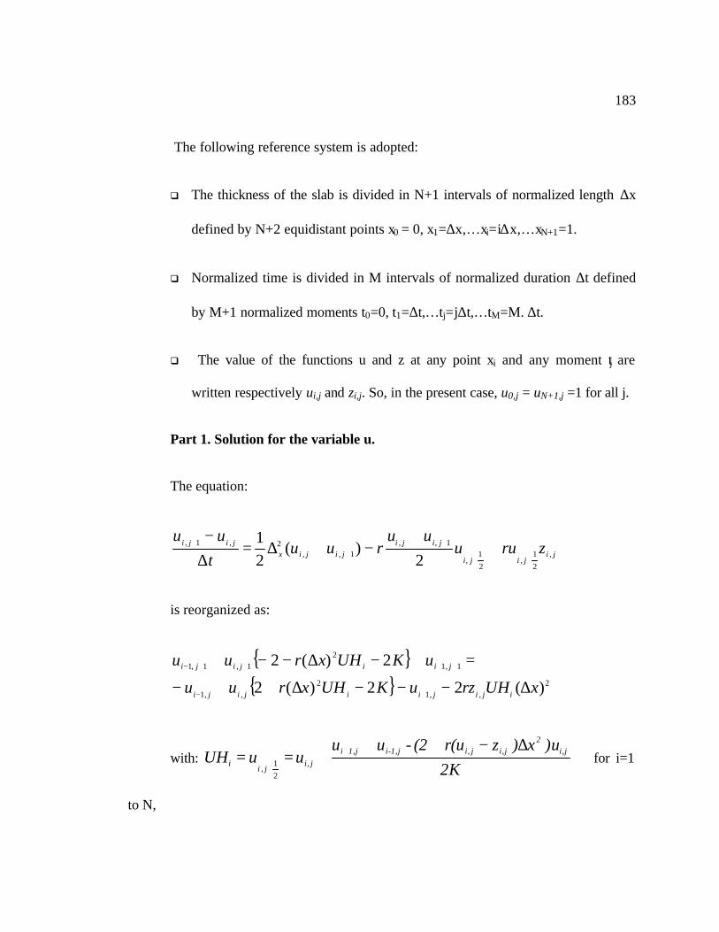
183

The following reference system is adopted:

q The thickness of the slab is divided in N+1 intervals of normalized length ∆x

defined by N+2 equidistant points x0 = 0, x1=∆x,…xi=i∆x,…xN+1=1.

q Normalized time is divided in M intervals of normalized duration ∆t defined

by M+1 normalized moments t0=0, t1=∆t,…tj=j∆t,…tM=M. ∆t.

q The value of the functions u and z at any point xi and any moment tj are

written respectively ui,j and zi,j. So, in the present case, u0,j = uN+1,j =1 for all j.

Part 1. Solution for the variable u.

The equation:

jijiji

jijijijix

jiji zruuuu

ruut

uu,

21

,21

,

1,,1,,

2,1,

2)(

21

++

++

+ ++

−+∆=∆−

is reorganized as:

{ }{ } 2

,,12

,,1

1,12

1,1,1

)(22)(2

2)(2

xUHrzuKUHxruu

uKUHxruu

ijijiijiji

jiijiji

∆−−−∆++−

=+−∆−−+

+−

++++−

with: 2K

)ux)z(ur(2-uuuuUH ji,

2ji,ji,j1,-ij1,i

ji,ji

i

∆−+++== +

+21

, for i=1

to N,

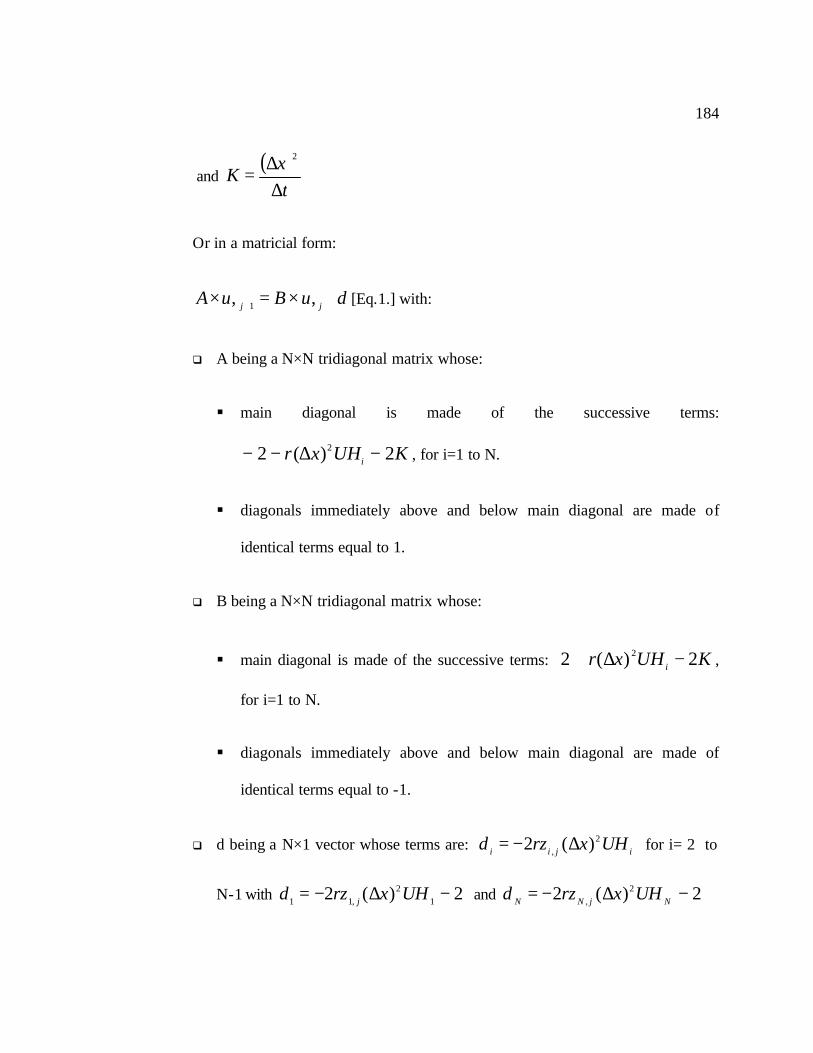
184

and ( )

tx

K∆

∆=

2

Or in a matricial form:

duBuA jj +×=× + ,, 1 [Eq.1.] with:

q A being a N×N tridiagonal matrix whose:

§ main diagonal is made of the successive terms:

KUHxr i 2)(2 2 −∆−− , for i=1 to N.

§ diagonals immediately above and below main diagonal are made of

identical terms equal to 1.

q B being a N×N tridiagonal matrix whose:

§ main diagonal is made of the successive terms: KUHxr i 2)(2 2 −∆+ ,

for i=1 to N.

§ diagonals immediately above and below main diagonal are made of

identical terms equal to -1.

q d being a N×1 vector whose terms are: ijii UHxrzd 2, )(2 ∆−= for i= 2 to

N-1 with 2)(2 12

,11 −∆−= UHxrzd j and 2)(2 2, −∆−= NjNN UHxrzd

185

q u,j+1 and u,j being the N×1 vectors representing u respectively at times j+1 and

j for i=1 to N.

The equation 1.is solved for each time increment, the matrices and vector A, B

and d being re-evaluated, using the “left-division” operator of Matlab:

( )duBAu jj +×=+ ,\, 1

The efficiency of the method can be improved by considering the symmetry of the

problem with respect to the median plane of the slab:

x)-u(1u(x) or X)-U(LU(X) == for all t. Thus it is possible to compute all

variables for the interval x=[0,½] only.

Subsequently, the reference system and terms of Equation 1.are modified as

follows:

q The half-thickness of the slab is divided in N intervals of normalized length

∆x defined by N+1 equidistant points x0 = 0, x1=∆x,…xi=i∆x,…xN=½.

q The expression for the forward projection of the function u to half- level of

time, at xN=½ becomes:

2K

)ux)z(u(2-u2u jN,

2jN,jN,j1,-N

jN,21

,

∆−++==

+

ruUH

jNN

186

q For the matrices A and B, the term at row N and column (N-1) becomes

respectively 2 and –2.

q For the vector d, dN takes now the same expression as di; d1 and di keeps the

same expression.

Part 2. Solution for the variable z.

Apart from the analytical solution, the values of the variable z can be computed

using the exponential form of the finite difference analog of the solution of Fick’s

equation, coupled with sub- interval time step elimination. Instead of the classical Crank-

Nicolson formula:

)(21

1,,2,1,

++ +∆=∆

−jijix

jiji zzt

zz, the following form is implemented:

−−−= +−

+ji

jijijijiji z

zzzRzz

,

,1,1,,1,

2exp ,

where R is the Fourier number, being equal to, in the case of the adimensional

form: ( ) Kx

tR 12 =

∆∆= .

In the case where the initial conditions are such that z =0 at all internal points, the

so-called substitution method will suffice to circumvent the problem: let a new variable

187

be zzz −= 0 , with z0 being different from 0 (for example, the value of z at the

boundary).

When zi,j is small, it is possible to use the first two terms of the Taylor expansion

of zi,j+1, which is less costly in term of computation time:

jijijiji RzzRRzz ,1,,11, )21( +−+ +−+= .

The latter expression is also useful when the problem of zi,j = 0 arises in the

exponential form.

The sub- interval time step elimination consists in dividing each successive time

interval ∆t of indice j, into p equal virtual sub- intervals. For each of them, the values of z

are computed, used for the next sub- interval, but not stored in memory, except for the last

one, that is assigned to the time increment j+1. Since the duration of the sub- intervals is

smaller than the duration of the time interval ∆t, a reduced Fourier number Rc is used.

The algorithm of the exponential method coupled with sub- interval time step elimination

is as follows:

pjiji zz ,1, =+ ,

with

−−−=

−

−+

−−

−−

1,

1,1

1,1

1,1

,,

2exp

kji

kji

kji

kji

ck

jik

ji z

zzzRzz for k =1 to p and

188

pR

Rc = with

=

fRR

p int +1,

“int” rounding to the lower nearest integer and Rf being a value of Fourier

number not greater than ½.

Since the exponential method is explicite, it is not unconditionnally stable. The

sub- interval time step elimination enables to run the method with higher Fourier numbers

without instability.

APPENDIX B

MATLAB PROGRAM FOR NUMERICAL SOLUTION PRESENTED IN

APPENDIX A

190

L=25e-3;% thickness of slab (meters) D=1e-12; % permeability coefficient (m^2/s) k=1e-8; % rate constant of reaction (mol U0=35.2;% sulfates initial concentration Ca=252.3;% calcium aluminates initial concentration r=k*L^2*U0/(3*D); p=-r; M=50 ;% number of time increments. N=25;% number of distance increments. dx=0.5/(N+0); dt=dx*0.08; K=dx^2/dt; l=[0:N+0];x=dx*l; u=[1;zeros(N,1)];%initialize u cal=(Ca/U0)*ones(N+1,1);%initialize [cal] z0=-3*Ca/U0; rf1=dt/dx^2; rf2=0.4;pbhat=fix(rf1/rf2)+1; rc=rf1/pbhat; z=z0*ones(N+1,1);%initialize Z dm=[rc*1;zeros(N-1,1)];% compute terms of vector d , then matrix Am Am=(+diag(rc*ones(N-1,1),1)+ diag(rc*ones(N-1,1),-1)+diag((1-

2*rc)*ones(N,1))); Am(N,N-1)=2*rc; for j=[1:M]% begin iterations zz=z(2:N+1,j); for kk=[1:pbhat] % VSIET procedure zz=Am*zz+dm; end z(2:N+1,j+1)=zz; z(1,j+1)=1; end for j=[1:M]% begin iterations % call analytical solution of Fick's 2nd law % compute forward projection of u to half-level of time UH(N)=u(N+1,j)+(2*u(N,j)-

(2+(r*u(N+1,j)+p*z(N+1,j+1))*dx^2)*u(N+1,j))/(2*K); for i=[2:N] UH(i-1)=u(i,j)+(u(i+1,j)+u(i-1,j)-

(2+(r*u(i,j)+p*z(i,j+1))*dx^2)*u(i,j))/(2*K); end % compute terms of main diagonals of matrices A and B a=-r*UH*dx^2-2*(1+K); b=2+r*UH*dx^2-2*K; % compute terms of vector d d(1)= 2*p*z(2,j+1)*dx^2*UH(1)-2 ; d(2:N)= 2*p*z(3:N+1,j+1)*dx^2.*(UH(2:N))'; % build matrices A and B A=sparse(diag(ones(N-1,1),1)+ diag(ones(N-1,1),-1)+diag(a)); A(N,N-1)=2; B=sparse(-diag(ones(N-1,1),1)-diag(ones(N-1,1),-1)+diag(b)); B(N,N-1)=-2; % solve system u(2:N+1,j+1)=A\(B*u(2:N+1,j)+d'); u(1,j+1)=1; % compute [cal] cal(2:N+1,j+1)=(u(2:N+1,j+1)-z(2:N+1,j+1))/3; if cal(end,j+1)<=0.01 break,toc,sounds(0) end if rem(j,5)==0 % pick here number of plots

191

plot(x,u(:,j),'r',x,cal(:,j),':'),axis ([0 0.5 0 Ca/U0]); hold on end end hold off

APPENDIX C

SOLUTION OF THE FINITE DIFFERENCE SCHEME FOR COMPOSITE

MATERIAL

193

The following reference system adopted in Appendix A is modified as follows:

q The half-thickness of the slab is divided in two intervals defined by the points

X0 = 0, XS=(S/N)×(L/2)and XN+1=L/2.

q The diffusion coefficient takes the values D1 and D2 respectively in the

intervals [X0 , XS] and [XS, XN+1].

At any given time T, the flux across the interface can be written:

xUDFand

xUDF

∂∂−=

∂∂−= 2

21

1

with U1 and U2 being the expression of U in the intervals [X0 , XS] and [XS, XN+1].

Also, at the interface: SSS UXUXU == )()( 21 .

These equations constitute the so-called “junction conditions”.

Let’s imagine that U1 takes a fictitious value US+1 in the interval [XS, XN+1] and

that U2 takes a fic titious value US-1 in the interval [X0 , XS] (see Figure C-1).

194

Figure C-1. Method of fictitious values.

From now on, the indices 1 and 2 for function U, relevant to the two media of

diffusivity D1 and D2, will be omitted for simplification of the equations, knowing

implicitely in which interval each expression is valid.

The analogues for the flux equations are respectively:

FXUU

D

FXUUD

SS

SS

−=∆−

−=∆−

−+

−+

2

211

2

111

The principle of the method is to isolate then eliminate the two fictitious values of

U:

0 X

plane of symmetry

L/2

U

XS XS-1 XS+1

∆X ∆X

US-1

US+1 US

D1 D2

195

211

1

11

2

2

DXF

UU

DXF

UU

SS

SS

∆+=

∆−=

+−

−+

Since these two equations are valid at any moment, it is possible to write them at

T=j∆T and T=(j+1)∆T (thus we get four fictitious values):

2

1,11,1

2,1,1

1

1,11,1

1,1,1

2

2

2

2

DXF

UU

DXFUU

DXF

UU

DXF

UU

jSjS

jSjS

jSjS

jSjS

∆+=

∆+=

∆−=

∆−=

+++−

+−

+−++

−+

In a first approach, the scheme will be devised for the equation with no reaction

term: 2

2

XUD

TU

∂∂=

∂∂

.

The Crank-Nicolson analog for this equation is:

∆

+−+

∆

+−=

∂∂ +−+++−+

2

1,11,1,1

2

,1,,1

)(

2

)(

2

2 X

UUU

X

UUUDTU jijijijijiji

For i=S, the equation above takes these forms, depending which medium is

considered:

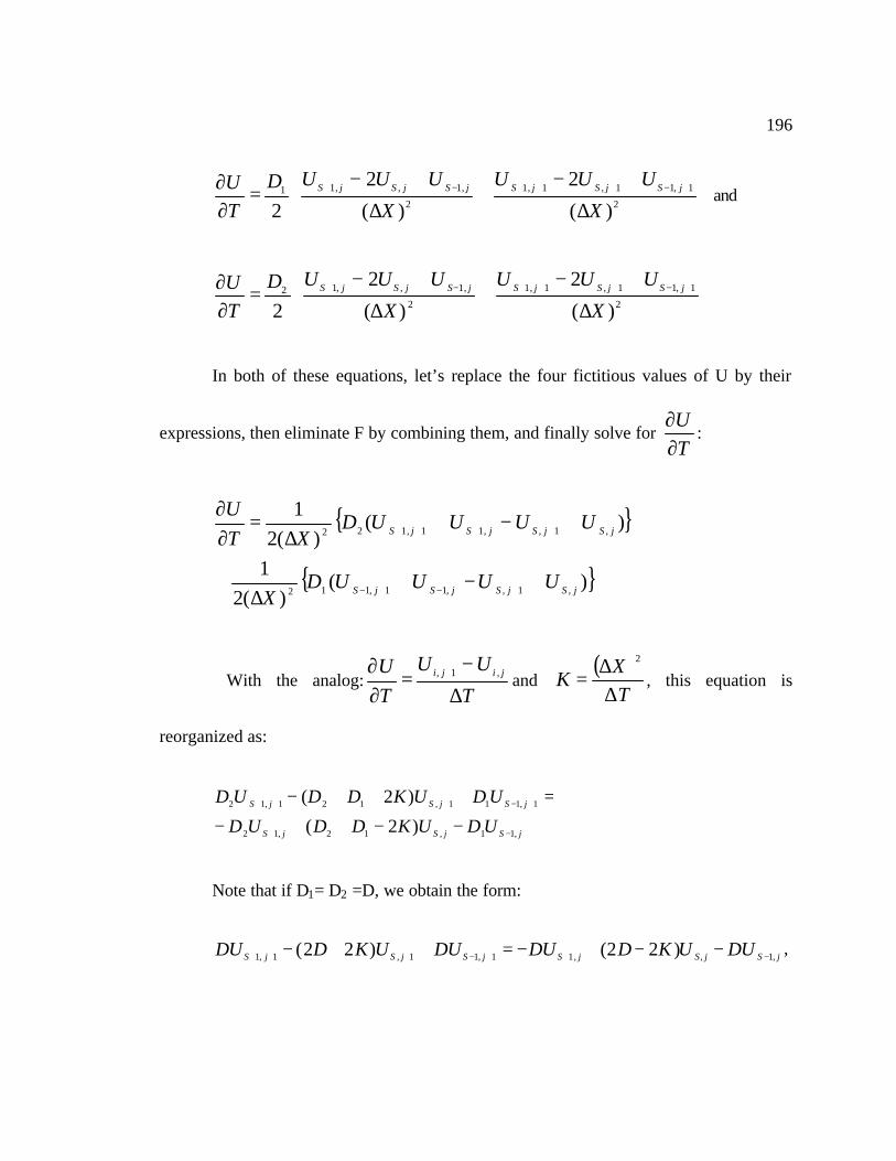
196

∆

+−+

∆

+−=

∂∂ +−+++−+

2

1,11,1,1

2

,1,,11

)(

2

)(

2

2 X

UUU

X

UUUDTU jSjSjSjSjSjS and

∆

+−+

∆

+−=

∂∂ +−+++−+

2

1,11,1,1

2

,1,,12

)(

2

)(

2

2 X

UUU

X

UUUDTU jSjSjSjSjSjS

In both of these equations, let’s replace the four fictitious values of U by their

expressions, then eliminate F by combining them, and finally solve for TU

∂∂

:

{ }

{ })()(2

1

)()(2

1

,1,,11,112

,1,,11,122

jSjSjSjS

jSjSjSjS

UUUUDX

UUUUDXT

U

+−+∆

+

++−+∆

=∂∂

+−+−

++++

With the analog:T

UU

TU jiji

∆

−=

∂∂ + ,1, and

( )T

XK

∆∆

=2

, this equation is

reorganized as:

jSjSjS

jSjSjS

UDUKDDUD

UDUKDDUD

,11,12,12

1,111,121,12

)2(

)2(

−+

+−+++

−−++−

=+++−

Note that if D1= D2 =D, we obtain the form:

jSjSjSjSjSjS DUUKDDUDUUKDDU ,1,,11,11,1,1 )22()22( −++−+++ −−+−=++− ,

197

which is the classical expression of the Crank-Nicolson method in a homogeneous

medium. This latter form will be adopted for i=1 to S-1 and i=S+1 to N with respectively

D= D1 and D= D2. Along with the particular equation devised for i=S, one obtains a

system of N equations with N unknowns. If each of the equations is divided by D2, the

system to be solved takes the form:

duBuA jj +×=× + ,, 1 , with:

q A being a N×N tridiagonal matrix whose:

§ main diagonal is made of the successive terms:

2

1 22D

KD −− for i=1 to S-1,

2

12 2D

KDD −−−, for i=S

2

2 22D

KD −− for i=S+1 to N.

§ diagonals immediately above and below main diagonal are made of

identical terms equal to 1, except for for the term at row S and column S-

1, which is equal to D1/ D2, and the term at row N and column (N-1)

which is equal to 2 (due to the limitation of the analysis to half the slab –

see Appendix A).

198

q B being a N×N tridiagonal matrix whose:

§ main diagonal is made of the successive terms:

2

1 22D

KD − for i=1 to S-1,

2

12 2D

KDD −+, for i=S

2

2 22D

KD − for i=S+1 to N.

§ diagonals immediately above and below main diagonal are made of

identical terms equal to 1, except for the term at row S and column S-1,

which is equal to ­D1/ D2, and the term at row N and column (N-1) which

is equal to -2.

q U,j+1 and U,j being the N×1 vectors representing U respectively at times j+1

and j for i=1 to N.

q d being a N×1 vector whose terms depends upon the boundary conditions.

Now let’s apply the same methodology to the equation system:

199

∂∂

=∂∂

∂∂

=∂∂

2

2

2

2

XZ

DTZ

3Z)-kU(U

-XU

DTU

in the composite medium.

For the equation 2

2

XZ

DTZ

∂∂

=∂∂

, we will carry out the scheme described in the first

part of this appendix, with the relevant initial and boundary conditions.

For the equation3

Z)-kU(U -2

2

XU

DTU

∂∂

=∂∂

, the method described in

Appendix A, along with the method of fictitious values described above, will be

implemented.

First, it is necessary to establish the expression for the forward projection of the

function U to half- level of time, for i=S:

∆

∂∂

+==+ 2,

,21

,

TtU

UUUHjS

jSjS

S

The fictitious values method yields:

)(622

12 ,,

,,1

1,

12,1

2jSjS

jSjSjSjSS UZ

TUkU

KD

UK

DDU

KD

UH −∆

++

+

−+= −+

200

For other values of i, it suffices to adapt the non-dimensional form of UH devised

in Appendix A, with the relevant value of D depending on i.

For the analog of the equation3

Z)-kU(U -2

2

XU

DTU

∂∂

=∂∂

at i=S, the finite

difference expression obtained for 2

2

XU

DTU

∂∂

=∂∂

(after division by D2) is modified

as follows:

q a term 2

2

3)(D

UHXk S∆is respectively subtracted from and added to the

coefficients of US,j+1 and US,j.

q a term2

2,

3

)(2

D

UHXkZ SjS ∆− is added to the right-hand term of the equation.

For other values of i, it is only needed to adapt the non-dimensional form devised

in Appendix A, with the relevant value of D.

Consequently the system can be reduced to the matricial form:

dUBUA jj +×=× + ,, 1 ,

with A, B and d taking the same form as in Appendix A, except for i=S, and with

D=D1 for i=1 to S-1 and D=D2 for i= S+1 to N.

201

Note: the cases S=0 and S=1 need specific attention, because respectively of the

coincidence with and proximity of the external boundary, as well as the case S=N

because of the coincidence with the plane of symmetry (S=0 and S=N correspond to the

homogeneous medium case).

The codes corresponding to the scheme are presented in Appendix D.

APPENDIX D

MATLAB PROGRAM FOR NUMERICAL SOLUTION PRESENTED IN

APPENDIX C.

203

L=25e-3;% thickness of slab (meters) D=1e-12; % permeability coefficient (m^2/s) k=1e-8; % rate constant of reaction (mol U0=35.2;% sulfates initial concentration Ca=252.3;% cal initial concentration M=10000 ;% number of time increments. N=25;% number of distance increments. dX=0.5*L/(N+0);dT=dX*4e8; K=dX^2/dT; % "default" dt=dx*0.02*50/N for k=0 l=[0:N+0];X=dX*l; U=[U0;zeros(N,1)];%initialize U cal=Ca*ones(N+1,1);%initialize [cal] Z0=-3*Ca;Z=Z0*ones(N+1,1);%initialize Z a=-2*(1+K/D)*ones(N,1);b=2*(1-K/D)*ones(N,1); % compute terms of vector d d(1)= -2*(U0) ;d(2:N)= zeros(N-1,1); % build matrices A and B A=sparse(diag(ones(N-1,1),1)+ diag(ones(N-1,1),-1)+diag(a)); A(N,N-1)=2; B=sparse(-diag(ones(N-1,1),1)-diag(ones(N-1,1),-1)+diag(b)); B(N,N-1)=-2; for j=[1:M]% begin iterations % solve system Z(2:N+1,j+1)=A\(B*Z(2:N+1,j)+d'); Z(1,j+1)=U0; end for j=[1:M]% begin iterations % call analytical solution of Fick's 2nd law % compute forward projection of U to half-level of time. % take in account indice gap between U,Z and UH. UH(N)=U(N+1,j)+D*(U(N,j)-U(N+1,j))/K + dT*k*U(N+1,j)*(Z(N+1,j+1)-

U(N+1,j))/6; for i=[2:N] UH(i-1)=U(i,j)+D*(U(i+1,j)-2*U(i,j)+U(i-1,j))/(2*K)+

dT*k*U(i,j)*(Z(i,j+1)-U(i,j))/6; end % compute terms of main diagonals of matrices A and B a=-2*(1+k*dX^2*UH/(6*D)+K/D); b=2*(1+k*dX^2*UH/(6*D)-K/D); % compute terms of vector d d(1)= -2*(U0+k*dX^2*UH(1)*Z(2,j+1)/(3*D)) ; d(2:N)= -2*k*dX^2*Z(3:N+1,j+1).*(UH(2:N))'/(3*D); % build matrices A and B A=sparse(diag(ones(N-1,1),1)+ diag(ones(N-1,1),-1)+diag(a)); A(N,N-1)=2; B=sparse(-diag(ones(N-1,1),1)-diag(ones(N-1,1),-1)+diag(b)); B(N,N-1)=-2; % solve system U(2:N+1,j+1)=A\(B*U(2:N+1,j)+d'); U(1,j+1)=U0; % compute [cal] cal(2:N+1,j+1)=(U(2:N+1,j+1)-Z(2:N+1,j+1))/3; if cal(end,j+1)<=(0.01*U0) break,toc,sounds(0) end if rem(j,50)==0 % pick here number of plots plot(X,U(:,j),'bx',X,cal(:,j),'rx'),axis ([0 L/2 0 Ca]);hold on end end hold off

APPENDIX E

NUMERICAL SOLUTION FOR THE DIFFUSION EQUATION WITH NO

REACTION, WITH A MOVING BOUNDARY

205

At the start, the geometry of the problem is the same as in Appendix A

(homogeneous slab divided into a grid of N identical intervals delimited by N+1 points).

After, the first iteration (t=1.∆t), a boundary is created within the slab at a point XS

corresponding to a given concentration UC, which delimits two regions:

q for 0<X< XS, U>UC and D=D1.

q for XS<X<L/2, U<UC and D=D2 (original diffusivity of the slab at t=0).

These formulations are used for the next iteration to compute the new

concentration profile using the formulae established for the composite slab (Appendix C).

A new value of XS is determined, which modifies again the geometry of the problem. The

method is carried out until the moving boundary reaches the center of the slab. At that

point, the problem is simply this of a homogeneous material of diffusivity D1.

The difficulty which arises is the non-coincidence of the location of the moving

boundary between the two materials (point for which U=UC) and any point of the finite

difference grid, i.e. XS is not part of the set of points X0=0, X1=∆X,…Xi=i∆X,…XN=L/2,

but falls between two points Xi-1 and Xi. To remedy this situation, it is possible to shift

the entire grid, except the extreme points, so that XS is part of it. The value of XS is the

weighted average of Xi-1 and Xi. Since the points X = 0 and X =L/2 are invariant, this

means that a supplementary point and interval are being created, and the first and last

intervals are now shorter than ∆X (the sum of their length is equal to ∆X). Thus, the

indice of the point of abscissa L/2 is now N+1 (XN+1=L/2). These supplementary point

206

and interval are introduced after the first iteration, and then the internal points of the grid

are shifted to the right or to the left depending on the new location of the internal

boundary and on the position of the grid at the precedent iteration. Consequently, no

interval is greater than ∆X. Obviously, the indice of the point corresponding to the

boundary has to be incremented by one if the grid is shifted to the left.

The values of the concentration U at the points of the new grid are obtained

through cubic spline interpolation. The interpolated values of U are being used at the next

iteration, along with the new gr id. The Figure E-1 and Figure E-2 illustrate this

technique.

207

Figure E-1. Moving grid method. First iteration: first shift of the grid,

creation of a supplementary point. The interval [0, XS] will be considered having a

diffusivity D1 for the next iteration. The distance δ is characteristic of the position of

the new grid.

δ ∆X-δ

0 X

plane of symmetry

L/2

U

XS

∆X

UC

D2

original grid

new grid

computed point

interpolated point

208

Figure E-2. Iteration at T=j∆T: in this configuration the grid is shifted to the

left, the indice of the point corresponding to the internal boundary will be

incremented by one. The region of diffusivity D1 will be extended up to XS for the

next iteration. Interpolated values of U are computed and carried to the next

iteration, along with the new value of δ .

To implement the Crank-Nicolson finite difference scheme on the moving

boundary-moving grid problem, one has to write the analog of the partial differential

∆X-δ δ

0 L/2

U

XS

∆X

UC

D1 D2

X

previous grid

new grid

computed point

interpolated point

209

equation for each of the following cases depending on the configuration of the two

adjacent intervals related to each analog:

q Case 1: having the same length and not being separated by the boundary

between the two materials (standard case). This length is equal to ∆X except

for the two intervals separated by the plane of symmetry (i=N+1), for which

the length is equal to ∆X-δ.

q Case 2: having the same length and being separated by the internal boundary

(case treated in Appendix C).

q Case 3: not having the same length and not being separated by the internal

boundary.

q Case 4: not having the same length and being separated by the internal

boundary.

Case 3 and 4 are relevant to the first and last pairs of intervals. Since these

intervals are uneven, one must use now the most general form of the analogs for the

space derivative of U:

1

,1,1

, +

−+

∆+∆

−=

∂∂

ii

jiji

ji XX

UU

XU

)()(

211

,11,1,1

,2

2

++

−+++

∆+∆∆∆∆+∆+∆−∆

=

∂∂

iiii

jiijiiijii

ji XXXXUXUXXUX

XU

210

1: −−=∆ iii XXXwith

For case 3 and 4:

q at i=1, ∆Xi = δ and ∆Xi+1 = ∆X.

q at i=N, ∆Xi = ∆X and ∆Xi+1 = ∆X- δ.

For case 4, the equations are further complicated by the change of diffusivity

between the two intervals.

Due to the moving grid and boundary, the tridiagonal matrices A and B of the

equation duBuA jj +×=× + ,, 1 are modified for each iteration, until the moving boundary

has reached the mid-plane of the slab. Except for the first iteration, A and B are (N+1) ×

(N+1) matrices. The components of the diagonals are given in

211

Table E-1 to Table E-4 (except for the first iteration case which is trivial), depending on

the location of the moving boundary. The following notations are being used:

TX

KandXXT

XK

∆∆

=−∆=∆∆

∆=

22 ''', δ

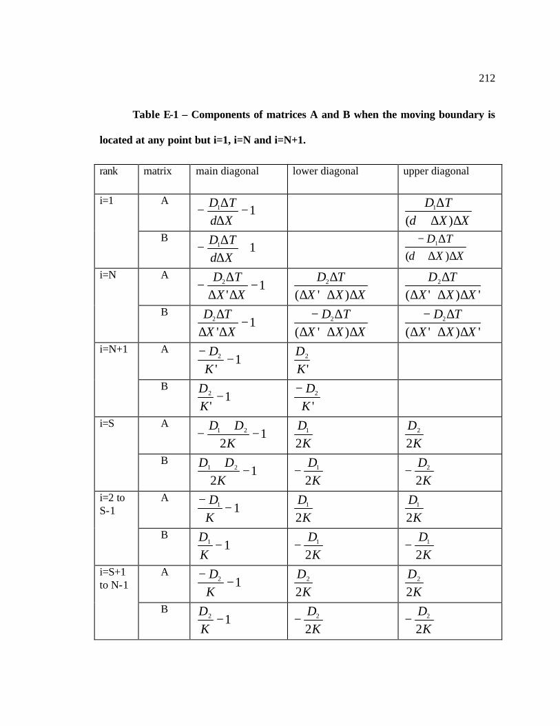
212

Table E-1 – Components of matrices A and B when the moving boundary is

located at any point but i=1, i=N and i=N+1.

rank matrix main diagonal lower diagonal upper diagonal

A 11 −

∆∆−XTD

δ

XXTD

∆∆+∆

)(1

δ

i=1

B 11 +

∆∆−XTD

δ

XXTD∆∆+

∆−)(

1

δ

A 1

'2 −

∆∆∆

−XXTD

XXX

TD∆∆+∆

∆)'(

2 ')'(

2

XXXTD

∆∆+∆∆

i=N

B 1

'2 −

∆∆∆

XXTD

XXX

TD∆∆+∆

∆−)'(

2 ')'(

2

XXXTD∆∆+∆

∆−

A 1

'2 −

−KD

'2

KD

i=N+1

B 1

'2 −

KD

'2

KD−

A 1

221 −

+−

KDD

K

D2

1 K

D2

2 i=S

B 1

221 −

+K

DD

KD2

1− K

D2

2−

A 11 −

−KD

K

D2

1 K

D2

1 i=2 to S-1

B 11 −

KD

K

D2

1− K

D2

1−

A 12 −

−KD

K

D2

2 K

D2

2 i=S+1 to N-1

B 12 −

KD

K

D2

2− K

D2

2−

213

Table E-2. Components of matrices A and B when the moving boundary is

located at point i=1.

rank matrix main diagonal lower diagonal upper diagonal

A 121 −

∆+

∆+∆−

XDD

XT

δδ

XTD

∆∆

δδ2

i=1

B 121 −

∆+

∆+∆

XDD

XT

δδ

XTD

∆∆

−δ

δ2

A 1

'2 −

∆∆∆

−XXTD

XXX

TD∆∆+∆

∆)'(

2

')'(

2

XXXTD

∆∆+∆∆

i=N

B 1

'2 −

∆∆∆

XXTD

XXX

TD∆∆+∆

∆−)'(

2

')'(

2

XXXTD∆∆+∆

∆−

A 1

'2 −

−KD

'2

KD

i=N+1

B 1

'2 −

KD

'2

KD−

A 12 −

−KD

K

D2

2

KD2

2

i=2 to N-1

B 12 −

KD

K

D2

2− K

D2

2−

214

Table E-3. Components of matrices A and B when the moving boundary is

located at point i=N.

rank matrix main diagonal lower diagonal upper diagonal

A 11 −

∆∆−XTD

δ

XXTD

∆∆+∆

)(1

δ

i=1

B 11 +

∆∆−XTD

δ

XXTD∆∆+

∆−)(

1

δ

A 1

''21 −

∆+

∆∆+∆∆−

XD

XD

XXT

XXX

TD∆∆+∆

∆)'(

1

')'(2

XXXTD

∆∆+∆∆

i=N

B 1

''21 −

∆+

∆∆+∆∆

XD

XD

XXT

XXX

TD∆∆+∆

∆−)'(

1

')'(2

XXXTD∆∆+∆

∆−

A 1

'2 −

−KD

'2

KD

i=N+1

B 1

'2 −

KD

'2

KD−

A 11 −

−KD

K

D2

1

KD2

1

i=2 to N-1

B 11 −

KD

K

D2

1− K

D2

1−

215

Table E-4. Components of matrices A and B when the moving boundary has

reached the mid-plane of the slab (i=N+1).

rank matrix main diagonal lower diagonal upper diagonal

A 11 −

∆∆−XTD

δ

XXTD

∆∆+∆

)(1

δ

i=1

B 11 +

∆∆−XTD

δ

XXTD∆∆+

∆−)(

1

δ

A 1

'1 −

∆∆∆

−XX

TD

XXXTD

∆∆+∆∆

)'(1

')'(

1

XXXTD

∆∆+∆∆

i=N

B 1

'1 −

∆∆∆

XXTD

XXX

TD∆∆+∆

∆−)'(

1

')'(1

XXXTD

∆∆+∆∆−

A 1

'1 −

−KD

'

1

KD

i=N+1

B 1

'1 −

KD

'

1

KD−

A 11 −

−KD

K

D2

1

KD2

1

i=2 to N-1

B 11 −

KD

K

D2

1− K

D2

1−

The expression of the vector d, which contains N+1 zeros except for the first term,

is the same for all the situations considered in Table E-1 to Table E-4, and is given by:

216

120)()(

2)1( 10 +==

+∆∆−

= NtoiforidandX

TDUd

δδ

The Matlab program implementing the method is presented in Appendix F.

To validate the method presented in this Appendix, it is possible to compare its

results to the results given by the analytical solution obtained for the same problem

applied to a semi- infinite solid. As long as the migrating ions have not reached the mid-

plane of the slab, the problem is identical to that of the semi- infinite solid, so the

numerical and analytical solution can be compared in that time interval.

In the analytical solution, the position of the moving boundary is given by:

TkTX S =)( , with k a constant depending on D1, D2, U0, U∝ and UC, and

determined by solving numerically the equation resulting from the application of the

boundary conditions.

The concentration profile is given by two functions U1 and U2 such as:

SXXforTD

XerfCUU <<+= 0

2 1

101

+∞<<+= ∞ XXforTD

XerfcCUU S

2

22 2

217

with U∝ being the concentration at large distances, and C1 and C2 two constants

depending on respectively D1, UC, k, U0 and D2, UC, k, U∝. The constants C1 and C2 are

obtained from the application of the boundary conditions.

In our case U∝ =0, and we will use the following values to compare the analytical

and numerical solutions:

D1= 10-10 m2/s, D2= 10-11 m2/s, U0=35.2 mol/m3 and UC=U0/2. With these values,

ones obtains: k =1.1869×10-5, C1 = -29.3980, C2 = 2.2125 ×103.

Figure E-3 and Figure E-4 show that the two methods are in good agreement for

the variation of the location of the moving boundary with time as well as for the

evolution of the concentration profile with time.

218

Figure E-3. Variation of the location of the moving boundary with time.

0 0.5 1 1.5 2 2.5 3 3.5 4 4.5 5

x 105

0

1

2

3

4

5

6

7

8

9x 10

-3

time (s)

loca

tion

of m

ovin

g bo

unda

ry (

m)

numerical solutionanalytical solution

219

Figure E-4. Evolution of the concentration profile with time.

Generalization to the case of continuous diffusivity:

Each layer comprised between the abscissa Xi and Xi+1 has a diffusivity Di,j,

updated at each time increment (with Di,j = D2 in the uncracked zone). Consequently, it is

sufficient to have two different kinds of equations, depending on whether the consecutive

space intervals considered are even or uneven. For example, in the case of even

consecutive intervals, Fick’s equation takes the form:

jijijijijijiji

jijijijijijiji

UDUKDDUD

UDUKDDUD

,1,,,,1,1,1

1,1,1,,,11,1,1

)2(

)2(

−+++

+−+++++

−−++−

=+++−

0 0.002 0.004 0.006 0.008 0.01 0.0120

5

10

15

20

25

30

35

abscissa (m)

conc

entr

atio

n (m

ol/m

3 )numerical solutionanalytical solution

220

Thus, it is easy to adapt the values of the preceding tables by replacing D1 and D2

by the relevant value of D (Di,j or Di+1,j), using only the cases i=S and i=N+1, for the

latter only DN+1,j being used.

221

APPENDIX F

MATLAB PROGRAM FOR NUMERICAL SOLUTION PRESENTED IN

APPENDIX E

222

L=25e-3;% thickness of slab (meters) D1=1e-11;D2=1e-12; % permeability coefficient (m^2/s) U0=35.2;% sulfates initial concentration M=500 ;Nplot=M/5;% number of time increments and plots. N=25;% number of distance increments. dX=0.5*L/N;dT=dX*2e7;S=0; K=dX^2/dT;X=dX*[0:N];X=X'; U=[U0;zeros(N,1)];%initialize U for j=[1:M]% begin iterations switch S % redirect to sub-routines case 0 mbmgs0 % call sub-routine for S=0 case 1 mbmgs1 % call sub-routine for S=1 case N mbmgsN% call sub-routine for S=N case N+1 mbmgsN1 % call sub-routine for S=N+1 otherwise mbmgsi % call sub-routine for other values of S end if j==1 % special case because there is one less X than later ii=min(find(U(:,j+1)<=U0/2));% criterion for boundary motion X_int(j)=interp1([U(ii-1,j+1),U(ii,j+1)],[X(ii-1),X(ii)],U0/2); ds=X_int(j)-X(ii-1);del(j)=ds;% compute gap dX1=dX-ds;K1=dX1^2/dT; S=1;% define material as composite X_initial=X; X(:,j+1)=X(:,j)+ds;%shift X to left X(N+1,j+1)=L/2;% reset last X = L/2 X=[[0,0];X];% reset first X = 0 and one fictitious component to

match future size U1(:,j)=U(:,j+1);% old U U=[[U0,U0];U];% add one fictitious component to match future size U(:,j+1)=interp1(X_initial,U1(:,j),X(:,j+1),'spline'); X_initial=[0;X_initial];% add one fictitious component to match

future size U1=[0;U1];% add one fictitious component to match future size else % inner test for all j>1 ii=min(find(U(:,j+1)<=U0/2));% criterion for boundary motion if isempty(ii)==1 % test for homogeneous material S=N+1; else % implement interpolation, moving grid method X_int(j)=interp1([U(ii-1,j+1),U(ii,j+1)],[X(ii-

1,j),X(ii,j)],U0/2); del(j)=X_int(j)-X(ii-1,j); X_initial(:,j)=X(:,j); X(:,j+1)=X(:,j)+del(j); if X(2,j+1)>dX X(:,j+1)=X(:,j)-(dX-del(j)); X(1,j+1)=0; X(N+2,j+1)=L/2; S=S+1; else X(1,j+1)=0; X(N+2,j+1)=L/2; end U1(:,j)=U(:,j+1); U(:,j+1)=interp1(X_initial(:,j),U1(:,j),X(:,j+1),'spline');

223

ds=X(2,j+1);dX1=dX-ds;K1=dX1^2/dT; end % end test on ii end % end test on j==1 if rem(j,Nplot)==0 % pick here number of plots % plot(X_initial(:,j),U1(:,j),'r'),axis ([0 L/2 0 U0]);hold on if size(U)==size(X)% take in account fact that grid is fixed at S=N+1 plot(X(:,j+1),U(:,j+1),'bx-'),hold on else plot(X(:,end),U(:,j+1),'r'),hold on end end SS(j)=S; end % end iteration j X_=[0,L/2];y=[U0/2,U0/2];% plot line U=U0/2 plot(X_,y,'k:') axis ([0 L/2 0 U0]); compact hold off SUBROUTINE “mbmgs0”

a=-2*(1+K/D2)*ones(N,1); b=2*(1-K/D2)*ones(N,1); c_left=ones(N-1,1); c_right=ones(N-1,1); d(1)= -2*(U0) ; d(2:N)= zeros(N-1,1); % build matrices A and B A=sparse(diag(c_left,-1)+ diag(ones(N-1,1),+1)+diag(a)); A(N,N-1)=2; B=sparse(-diag(c_right,-1)-diag(ones(N-1,1),+1)+diag(b)); B(N,N-1)=-2; % solve system U(2:N+1,j+1)=A\(B*U(2:N+1,j)+d'); U(1,j+1)=U0;

SUBROUTINE “mbmgS1”

% build main diagonal of A a=(D2/K+1)*ones(N+1,1);a(1)=dT*(D2/dX+D1/ds)/(ds+dX)+1; a(N)=D2*dT/(dX*dX1)+1;a(N+1)=D2/K1+1; % build lower diagonal of A low_a=(D2/(2*K))*ones(N,1); low_a(N-1)=D2*dT/dX/(dX+dX1); low_a(N)=D2/K1; % build upper diagonal of A upp_a=(D2/(2*K))*ones(N,1); upp_a(N)=D2*dT/dX1/(dX+dX1); upp_a(1)=D2*ds*dT*(1/ds+1/dX)/(ds+dX)^2; % build A A=sparse(-diag(a)+diag(low_a,-1)+diag(upp_a,1)); % build main diagonal of B b=(D2/K-1)*ones(N+1,1);b(1)=dT*(D2/dX+D1/ds)/(ds+dX)-1; b(N)=D2*dT/(dX*dX1)-1;b(N+1)=D2/K1-1; % build lower diagonal of B

224

low_b=-(D2/(2*K))*ones(N,1); low_b(N-1)=-D2*dT/dX/(dX+dX1); low_b(N)=-D2/K1; % build upper diagonal of B upp_b=-(D2/(2*K))*ones(N,1); upp_b(N)=-D2*dT/dX1/(dX+dX1); upp_b(1)=-D2*ds*dT*(1/ds+1/dX)/(ds+dX)^2; B=sparse(diag(b)+diag(low_b,-1)+diag(upp_b,1)); d= zeros(N+1,1); d(1)=-2*D1*U0*dT*dX*(1/dX+1/ds)/(dX+ds)^2; % solve system U(2:N+2,j+1)=A\(B*U(2:N+2,j)+d); U(1,j+1)=U0;

SUBROUTINE “mbmgSi”

% build main diagonal of A N2=N+1-S; a1=(1+D1/K)*ones(S-1,1);a2=(1+D2/K)*ones(N2,1); a=[a1;+((D2+D1)/(2*K)+1);a2]; a(1)=dT*D1/(dX*ds)+1; a(N)=D2*dT/(dX*dX1)+1;a(N+1)=D2/K1+1; % build lower diagonal of A low_a1=(D1/(2*K))*ones(S-1,1);low_a2=(D2/(2*K))*ones(N2,1); low_a=[low_a1;low_a2];low_a(S-1)=D1/2/K; low_a(N-1)=D2*dT/dX/(dX+dX1); low_a(N)=D2/K1; % build upper diagonal of A upp_a1=(D1/(2*K))*ones(S-1,1);upp_a2=(D2/(2*K))*ones(N2,1); upp_a=[upp_a1;upp_a2];upp_a(S)=D2/2/K; upp_a(N)=D2*dT/dX1/(dX+dX1); upp_a(1)=D1*dT/dX/(ds+dX); % build A A=sparse(-diag(a)+diag(low_a,-1)+diag(upp_a,1)); % build main diagonal of B b1=(-1+D1/K)*ones(S-1,1);b2=(-1+D2/K)*ones(N2,1); b=[b1;((D2+D1)/(2*K)-1);b2]; b(1)=dT*D1/(dX*ds)-1; b(N)=D2*dT/(dX*dX1)-1;b(N+1)=D2/K1-1; % build lower diagonal of B low_b1=(-D1/(2*K))*ones(S-1,1);low_b2=(-D2/(2*K))*ones(N2,1); low_b=[low_b1;low_b2];low_b(S-1)=-D1/2/K; low_b(N-1)=-D2*dT/dX/(dX+dX1); low_b(N)=-D2/K1; % build upper diagonal of B upp_b1=(-D1/(2*K))*ones(S-1,1);upp_b2=(-D2/(2*K))*ones(N2,1); upp_b=[upp_b1;upp_b2];upp_b(S)=-D2/2/K; upp_b(N)=-D2*dT/dX1/(dX+dX1); upp_b(1)=-D1*dT/dX/(ds+dX); % build B B=sparse(diag(b)+diag(low_b,-1)+diag(upp_b,1)); d= zeros(N+1,1); d(1)=-2*D1*U0*dT/(dX+ds)/ds; % solve system U(2:N+2,j+1)=A\(B*U(2:N+2,j)+d); U(1,j+1)=U0;

225

SUBROUTINE “mbmgSN”

% build main diagonal of A a=(1+D1/K)*ones(N+1,1); a(1)=dT*D1/(dX*ds)+1; a(N)=dT*(D2*dX+D1*dX1)/(dX*dX1*(dX+dX1))+1;a(N+1)=D2/K1+1; % build lower diagonal of A low_a=(D1/(2*K))*ones(N,1); low_a(N-1)=D1*dT/dX/(dX+dX1); low_a(N)=D2/K1; % build upper diagonal of A upp_a=(D1/(2*K))*ones(N,1); upp_a(N)=D2*dT/dX1/(dX+dX1); upp_a(1)=D1*dT/dX/(ds+dX); % build A A=sparse(-diag(a)+diag(low_a,-1)+diag(upp_a,1)); % build main diagonal of B b=(D1/K-1)*ones(N+1,1); b(1)=dT*D1/(dX*ds)-1; b(N)=dT*(D2*dX+D1*dX1)/(dX*dX1*(dX+dX1))-1;b(N+1)=D2/K1-1; % build lower diagonal of B low_b=(-D1/(2*K))*ones(S-1,1); low_b(N-1)=-D1*dT/dX/(dX+dX1); low_b(N)=-D2/K1; % build upper diagonal of B upp_b=(-D1/(2*K))*ones(N,1); upp_b(N)=-D2*dT/dX1/(dX+dX1); upp_b(1)=-D1*dT/dX/(ds+dX); % build B B=sparse(diag(b)+diag(low_b,-1)+diag(upp_b,1)); d= zeros(N+1,1); d(1)=-2*D1*U0*dT/(dX+ds)/ds; % solve system U(2:N+2,j+1)=A\(B*U(2:N+2,j)+d); U(1,j+1)=U0;

226

SUBROUTINE “mbmgSN1”

% build main diagonal of A a=(1+D1/K)*ones(N+1,1); a(1)=dT*D1/(dX*ds)+1; a(N)=D1*dT/(dX*dX1)+1;a(N+1)=D1/K1+1; % build lower diagonal of A low_a=(D1/(2*K))*ones(N,1); low_a(N-1)=D1*dT/dX/(dX+dX1); low_a(N)=D1/K1; % build upper diagonal of A upp_a=(D1/(2*K))*ones(N,1); upp_a(N)=D1*dT/dX1/(dX+dX1); upp_a(1)=D1*dT/dX/(ds+dX); % build A A=sparse(-diag(a)+diag(low_a,-1)+diag(upp_a,1)); % build main diagonal of B b=(-1+D1/K)*ones(N+1,1); b(1)=dT*D1/(dX*ds)-1; b(N)=D1*dT/(dX*dX1)-1;b(N+1)=D1/K1-1; % build lower diagonal of B low_b=(-D1/(2*K))*ones(N,1); low_b(N-1)=-D1*dT/dX/(dX+dX1); low_b(N)=-D1/K1; % build upper diagonal of B upp_b=(-D1/(2*K))*ones(N,1); upp_b(N)=-D1*dT/dX1/(dX+dX1); upp_b(1)=-D1*dT/dX/(ds+dX); % build B B=sparse(diag(b)+diag(low_b,-1)+diag(upp_b,1)); d= zeros(N+1,1); d(1)=-2*D1*U0*dT/(dX+ds)/ds; % solve system U(2:N+2,j+1)=A\(B*U(2:N+2,j)+d); U(1,j+1)=U0;

APPENDIX G

NUMERICAL SOLUTION FOR THE DIFFUSION-REACTION EQUATION

WITH A MOVING BOUNDARY.

228

The geometry of the problem is the same as in Appendix E. The methods to take

into account the change of diffusivity and to shift the grid as the internal boundary moves

are the same as exposed in Appendices C and E. In the other hand, the method of

Appendix A is used to solve the non-linear diffusion-reaction. First, it is necessary to

establish the expression for the forward projection of the function U to half- level of time:

∆

∂∂

+==+ 2,

,21

,

TtU

UUUHji

jiji

i ,

for each value of i and each location of the moving boundary.

For S=1 (moving boundary in between the two first intervals), one obtains:

q for i=1:

6)(

)(1

)(1111021

122

1

UZTUkX

TDUX

DDX

TU

XXTDU

UH−∆

++∆∆

+

∆+

+∆∆

−++∆∆

∆=

δδδδδ

q for i=N:

6)(

)'('1

)'('21221 NNNN

NN

N

UZTUkXXXTDU

XXTD

UXXX

TDUUH

−∆+

∆+∆∆∆

+

∆∆∆

−+∆+∆∆

∆= −+

q for i=N+1 (mid-slab), it suffices to adapt the non-dimensional form devised in

Appendix A, with D=D2 and replacing K by K’.

229

q for all other values of i, it suffices to adapt the non-dimensional form devised

in Appendix A, with the relevant value of D depending on i.

For S=N (moving boundary in between the two last intervals), one obtains:

q for i=1: replace D2 by D1 in the expression for S=1, i=1.

q for i=N:

6)(

)'(

''1

)'('

11

1221

NNNN

NN

N

UZTUkXXX

TDU

XD

XD

XXT

UXXX

TDUUH

−∆+

∆+∆∆∆

+

∆

+∆∆∆

∆−+

∆+∆∆∆

=

−

+

q for i=N+1, the expression is the same as for S=1, i=1.

q for all other values of i, the expression is the general dimensional form with

D=D1.

For S=N+1 (moving boundary has reached the mid-slab, which is now

homogeneous), one obtains:

q for i=1: the same expression as for S=N, i=1.

q for i=N: replace D2 by D1 in the expression for S=N, i=N.

q for i=N+1: replace D2 by D1 in the expression for S=1, i=N+1.

230

q for all other values of i, the expression is the general dimensional form with

D=D1.

When S takes any other value (except the trivial case S=0), the expression of UHi

are:

q for i=1: the same expression as for S=N, i=1.

q for i=N: the same expression as for S=1, i=N.

q for i=N+1: the same expression as for S=1, i=N+1.

q for i=S (and i≠1, i≠N, i≠N+1), i.e at the boundary, the expression is the same

as in Appendix C.

q for all other values of i, it suffices to adapt the non-dimensional form devised

in Appendix A, with the relevant value of D depending on i.

In all the expressions that precede, the second indice j has been omitted for the

sake of clarity, since all values of U and Z are expressed at this same time level.

Now, it is necessary to accomplish the same task on the diffusion-reaction

equation itself. Because of the method of linearization exposed in Appendix A, compared

to the case of diffusion with no reaction, only the terms of rank i are modified by the

introduction of the chemical reaction expression. Thus, only the main diagonal of both

matrices A and B and the vector d are concerned. With reference to Tables E-1 to E-4 of

231

Appendix E, the terms to be added to the terms of the main diagonals of A and B are

given in Table G-1 to Table G-4.

Table G-1. Terms to add to main diagonal terms of Table E-1.

rank A B

i=1

61TUHk∆

− 6

1TUHk∆+

i=N

6NTUHk∆

− 6

NTUHk∆+

i=N+1

61+∆

− NTUHk

61+∆

+ NTUHk

i=S

6STUHk∆

− 6

STUHk∆+

i=2 to S-1 6

iTUHk∆−

6iTUHk∆

+

i=S+1 to N-1 6

iTUHk∆−

6iTUHk∆

+

232

Table G-2. Terms to add to main diagonal terms of Table E-2.

rank A B

i=1

61TUHk∆

− 6

1TUHk∆+

i=N

6NTUHk∆

− 6

NTUHk∆+

i=N+1

61+∆

− NTUHk

61+∆

+ NTUHk

i=2 to N-1 6

iTUHk∆−

6iTUHk∆

+

Table G-3. Terms to add to main diagonal terms of Table E-3.

rank A B

i=1

61TUHk∆

− 6

1TUHk∆+

i=N

6NTUHk∆

− 6

NTUHk∆+

i=N+1

61+∆

− NTUHk

61+∆

+ NTUHk

i=2 to N-1 6

iTUHk∆−

6iTUHk∆

+

233

Table G-4. Terms to add to main diagonal terms of Table E-4.

rank A B

i=1

61TUHk∆

− 6

1TUHk∆+

i=N

6NTUHk∆

− 6

NTUHk∆+

i=N+1

61+∆

− NTUHk

61+∆

+ NTUHk

i=2 to N-1 6

iTUHk∆−

6iTUHk∆

+

For the vector d, the following term has to be added to the expression given in

Appendix E: 3

iiUHTZk∆− , for i=1 to N+1.

Generalization to the case of continuous diffusivity:

As for the problem described in Appendix E, it is possible to adapt the

expressions established for the discontinuous diffusivity case. For example, in the case of

even consecutive intervals, the expression for UH takes the form:

)(622

12 ,,

,,1

,,

,,1,1

,1jiji

jiji

jiji

jijiji

jii UZ

TUkU

K

DU

K

DDU

K

DUH −

∆++

+−+= −

++

+

All other expressions given for UH are transformed in a similar manner by

replacing D1 and D2 by the relevant value of D (Di,j or Di+1,j). The numerical scheme:

234

duBuA jj +×=× + ,, 1 , is then solved by using the tables of Appendix E, updated for the

continuous diffusivity case, with the additional terms for the main diagonal given in this

Appendix, being also updated for the continuous diffusivity case. The same methodology

is applied to vector d.

235

APPENDIX H: MATLAB PROGRAM FOR NUMERICAL SOLUTION

PRESENTED IN APPENDIX G.

236

L=25e-3;% thickness of slab (meters) D1=1e-11;D2=D1/10;%1e-12; % permeability coefficient (m^2/s) U0=35.2;% sulfates initial concentration alpha=268e-6/3.03; C=2;switch C % cal initial concentration case 1, Ca=8.15; case 2, Ca=82.5;case 3, Ca=252.3;end k=1e-7; %k=0;% rate constant of reaction (mol M=10;Nplot=M/M;% number of time increments and plots. N=25;% number of distance increments. dX=0.5*L/N;dT=dX*1e8;% 1e7 for 1e-11, 1e-12 K=dX^2/dT;X=dX*[0:N];X=X';S=0; U=[U0;zeros(N,1)];cal=Ca*ones(N+1,1);%initialize [cal],initialize U calr=Ca*ones(N+1,1);%initialize [cal]reacted Epsv=zeros(N+1,1);%initialize Epsv (one third of volumetric strain) Z0=-3*Ca;Z=Z0*ones(N+1,1);%initialize Z eps_B=200e-6; compute_Cx, % call program to determine Cx for j=[1:M]% begin iterations switch S % redirect to sub-routines case 0 mbzs0 % call sub-routine for S=0 case 1 mbzs1 % call sub-routine for S=1 case N mbzsN% call sub-routine for S=N case N+1 mbzsN1 % call sub-routine for S=N+1 otherwise mbzsi % call sub-routine for other values of S end switch S case 0 UH(N)=U(N+1,j)+D2*(U(N,j)-U(N+1,j))/K + dT*k*U(N+1,j)*(Z(N,j+1)-

U(N+1,j))/6; for i=[2:N] UH(i-1)=U(i,j)+D2*(U(i+1,j)-2*U(i,j)+... U(i-1,j))/(2*K)+ dT*k*U(i,j)*(Z(i,j+1)-U(i,j))/6; end case 1 % page 21. U2= U(3), U1=U(2), U0=U(1) UH(1)=U(3,j)*D2*dT/dX/(dX+ds)+U(2,j)*(1-

dT*(D1/ds+D2/dX)/(ds+dX))+... U0*D1*dT/ds/(dX+ds)+dT*k*U(2)*(Z(2,j+1)-U(2,j))/6; UH(N)=dT*D2*U(N+2,j)/dX1/(dX+dX1)+U(N+1,j)*(1-D2*dT/dX/dX1)+... dT*D2*U(N,j)/dX/(dX+dX1)+dT*k*U(N+1,j)*(Z(N+1,j+1)-U(N+1,j))/6; UH(N+1)=U(N+2,j)+D2*(U(N+1,j)-U(N+2,j))/K1 +... dT*k*U(N+2,j)*(Z(N+2,j+1)-U(N+2,j))/6; for i=[3:N] UH(i-1)=U(i,j)+D2*(U(i+1,j)-2*U(i,j)+U(i-1,j))/(2*K)+... dT*k*U(i,j)*(Z(i,j+1)-U(i,j))/6; end case N UH(1)=U(3,j)*D1*dT/dX/(dX+ds)+U(2,j)*(1-

dT*(D1/ds+D1/dX)/(ds+dX))+... U0*D1*dT/ds/(dX+ds)+dT*k*U(2)*(Z(2,j+1)-U(2,j))/6; for i=[3:N] UH(i-1)=U(i,j)+D1*(U(i+1,j)-2*U(i,j)+U(i-1,j))/(2*K)+... dT*k*U(i,j)*(Z(i,j+1)-U(i,j))/6; end

237

UH(N+1)=U(N+2,j)+D2*(U(N+1,j)-U(N+2,j))/K1 +... dT*k*U(N+2,j)*(Z(N+2,j+1)-U(N+2,j))/6; UH(N)=U(N+2,j)*D2*dT/dX1/(dX+dX1)+U(N+1,j)*(1-

dT*(D1/dX+D2/dX1)/(dX1+dX))+... dT*D1*U(N,j)/dX/(dX+dX1)+dT*k*U(N+1)*(Z(N+1,j+1)-U(N+1,j))/6; case N+1 UH(1)=U(3,j)*D1*dT/dX/(dX+ds)+U(2,j)*(1-

dT*(D1/ds+D1/dX)/(ds+dX))+... U0*D1*dT/ds/(dX+ds)+dT*k*U(2)*(Z(2,j+1)-U(2,j))/6; for i=[3:N] UH(i-1)=U(i,j)+D1*(U(i+1,j)-2*U(i,j)+U(i-1,j))/(2*K)+... dT*k*U(i,j)*(Z(i,j+1)-U(i,j))/6; end UH(N)=dT*D1*U(N+2,j)/dX1/(dX+dX1)+U(N+1,j)*(1-D1*dT/dX/dX1)+... dT*D1*U(N,j)/dX/(dX+dX1)+dT*k*U(N+1,j)*(Z(N+1,j+1)-U(N+1,j))/6; UH(N+1)=U(N+2,j)+D1*(U(N+1,j)-U(N+2,j))/K1 +... dT*k*U(N+2,j)*(Z(N+2,j+1)-U(N+2,j))/6; otherwise UH(1)=U(3,j)*D1*dT/dX/(dX+ds)+U(2,j)*(1-

dT*(D1/ds+D1/dX)/(ds+dX))+... U0*D1*dT/ds/(dX+ds)+dT*k*U(2)*(Z(2,j+1)-U(2,j))/6; UH(N)=dT*D2*U(N+2,j)/dX1/(dX+dX1)+U(N+1,j)*(1-D2*dT/dX/dX1)+... dT*D2*U(N,j)/dX/(dX+dX1)+dT*k*U(N+1,j)*(Z(N+1,j+1)-U(N+1,j))/6; UH(N+1)=U(N+2,j)+D2*(U(N+1,j)-U(N+2,j))/K1 +... dT*k*U(N+2,j)*(Z(N+2,j+1)-U(N+2,j))/6; UH(S)=D2*U(S+2,j)/(2*K)+U(S+1,j)*(1-

(D1+D2)/(2*K))+D1*U(S,j)/(2*K)... +dT*k*U(S+1,j)*(Z(S+1,j+1)-U(S+1,j))/6; for i=[3:S] UH(i-1)=U(i,j)+D1*(U(i+1,j)-2*U(i,j)+U(i-1,j))/(2*K)+... dT*k*U(i,j)*(Z(i,j+1)-U(i,j))/6; end for i=[S+2:N] UH(i-1)=U(i,j)+D2*(U(i+1,j)-2*U(i,j)+U(i-1,j))/(2*K)+... dT*k*U(i,j)*(Z(i,j+1)-U(i,j))/6; end end switch S % redirect to sub-routines that compute U case 0 mbUs0 % call sub-routine for S=0 case 1 mbUs1 % call sub-routine for S=1 case N mbUsN% call sub-routine for S=N case N+1 mbUsN1 % call sub-routine for S=N+1 otherwise mbUsi % call sub-routine for other values of S end if j==1 | S==0% special case because there is one less X than later cal(2:N+1,j+1)=(U(2:N+1,j+1)-Z(2:N+1,j+1))/3; ii=min(find((cal(:,j+1))>Cx));% criterion for boundary motion if isempty(ii)==1 % test for homogeneous material S=0; else X_int(j)=interp1([cal(ii-1,j+1),cal(ii,j+1)],[X(ii-

1),X(ii)],Cx); ds=X_int(j)-X(ii-1);del(j)=ds;% compute gap

238

dX1=dX-ds;K1=dX1^2/dT; S=1;% define material as composite

X_initial=X;% temporary variable defined X(:,j+1)=X(:,j)+ds;%shift X to left X(N+1,j+1)=L/2;% reset last X = L/2 X=[[0,0];X];% reset first X = 0 and one fictitious component to

match future size U1(:,j)=U(:,j+1);% old U U=[[U0,U0];U];% add one fictitious component to match future

size U(:,j+1)=interp1(X_initial,U1(:,j),X(:,j+1),'spline');%spline

interpolation X_initial=[0;X_initial];% add one fictitious component to match

future size U1=[0;U1];% add one fictitious component to match future size cal=[[0,0];cal];% add one fictitious component to match future

size end % end test for homogeneous material (first) elseif j>1 % inner test for all j>1 cal(2:N+2,j+1)=(U(2:N+2,j+1)-Z(2:N+2,j+1))/3; ii=min(find((cal(:,j+1))>Cx));% criterion for boundary motion if isempty(ii)==1 | S==N+1% test for homogeneous material S=N+1; % fix internal boundary at mid-slab else % implement interpolation, moving grid method X_int(j)=interp1([cal(ii-1,j+1),cal(ii,j+1)],[X(ii-

1,j),X(ii,j)],Cx); del(j)=X_int(j)-X(ii-1,j);% distance between location of mb and

next grid point X_initial(:,j)=X(:,j);% temporary variable defined X(:,j+1)=X(:,j)+del(j);% shift X to left if X(2,j+1)>dX % limitation of first interval to max. value: dX X(:,j+1)=X(:,j)-(dX-del(j)); X(1,j+1)=0;X(N+2,j+1)=L/2; S=S+1;% increment indice of moving boundary else X(1,j+1)=0;X(N+2,j+1)=L/2; end U1(:,j)=U(:,j+1); U(:,j+1)=interp1(X_initial(:,j),U1(:,j),X(:,j+1),'spline'); ds=X(2,j+1);dX1=dX-ds;K1=dX1^2/dT; end % end test for homogeneous material (second) end % end test on j==1 if cal(end,j+1)<=(0.01*U0) % test for end of reaction (exhaustion) break,toc,sounds(0) end % end test on exhaustion interpolZ % call subroutine to compute interpolated values of Z cal(2:N+2,j+1)=(U(2:N+2,j+1)-Z(2:N+2,j+1))/3;% compute interpolated

values calr(2:N+2,j+1)=Ca-cal(2:N+2,j+1);calr(1,j+1)=Ca;% deduce cal reacted if rem(j,Nplot)==0 % plotting routine if size(U)==size(X)% means that grid is still moving plot(X(:,j+1),U(:,j+1),'rx',X(:,j+1),calr(:,j+1),'bx:'),hold on hold on else % take in account fact that grid is fixed at S=N+1, % thus X is not updated anymore from this time on. plot(X(:,end),U(:,j+1),'r',X(:,end),calr(:,j+1),'b:'),hold on hold on end end % end test for plotting routine

239

SS(j)=S; end % end iteration on j

SUBROUTINE “mbUS0”

a=-2*(1+k*dX^2*UH/(6*D2)+K/D2); b=2*(1+k*dX^2*UH/(6*D2)-K/D2); c_left=ones(N-1,1); c_right=ones(N-1,1); d(1)= -2*(U0+k*dX^2*UH(1)*Z(2,j+1)/(3*D2)) ; d(2:N)= -2*k*dX^2*Z(3:N+1,j+1).*(UH(2:N))'/(3*D2); % build matrices A and B A=sparse(diag(c_left,-1)+ diag(ones(N-1,1),+1)+diag(a)); A(N,N-1)=2; B=sparse(-diag(c_right,-1)-diag(ones(N-1,1),+1)+diag(b)); B(N,N-1)=-2; % solve system U(2:N+1,j+1)=A\(B*U(2:N+1,j)+d'); U(1,j+1)=U0;

SUBROUTINE “mbUS1”

if j==2 UH=UH'; end % build main diagonal of A a=(D2/K+1)*ones(N+1,1)+k*UH*dT/6; a(1)=dT*(D2/dX+D1/ds)/(ds+dX)+1+k*dT*UH(1)/6; a(N)=D2*dT/(dX*dX1)+1+k*dT*UH(N)/6; a(N+1)=D2/K1+1+k*dT*UH(N+1)/6; % build lower diagonal of A low_a=(D2/(2*K))*ones(N,1); low_a(N-1)=D2*dT/dX/(dX+dX1); low_a(N)=D2/K1; % build upper diagonal of A upp_a=(D2/(2*K))*ones(N,1); upp_a(N)=D2*dT/dX1/(dX+dX1); upp_a(1)=D2*dT/dX/(ds+dX); % build A A=sparse(-diag(a)+diag(low_a,-1)+diag(upp_a,1)); % build main diagonal of B b=(D2/K-1)*ones(N+1,1)+k*UH*dT/6; b(1)=dT*(D2/dX+D1/ds)/(ds+dX)-1+k*dT*UH(1)/6; b(N)=D2*dT/(dX*dX1)-1;b(N+1)=D2/K1-1; % build lower diagonal of B low_b=-(D2/(2*K))*ones(N,1); low_b(N-1)=-D2*dT/dX/(dX+dX1); low_b(N)=-D2/K1; % build upper diagonal of B upp_b=-(D2/(2*K))*ones(N,1); upp_b(N)=-D2*dT/dX1/(dX+dX1); upp_b(1)=-D2*dT/dX/(ds+dX); B=sparse(diag(b)+diag(low_b,-1)+diag(upp_b,1));

240

d= -k*Z(2:N+2,j+1).*UH(:)*dT/3; d(1)=-2*D1*U0*dT/ds/(dX+ds)-k*Z(2,j+1).*UH(1)*dT/3; % solve system U(2:N+2,j+1)=A\(B*U(2:N+2,j)+d); U(1,j+1)=U0;

SUBROUTINE “mbUSi”

% build main diagonal of A N2=N+1-S; a1=(1+D1/K)*ones(S-1,1)+k*UH(1:S-1)*dT/6; a2=(1+D2/K)*ones(N2,1)+k*UH(S+1:N+1)*dT/6; a=[a1;+((D2+D1)/(2*K)+1+k*dT*UH(S)/6);a2]; a(1)=dT*D1/(dX*ds)+1+k*dT*UH(1)/6; a(N)=D2*dT/(dX*dX1)+1+k*UH(N)*dT/6; a(N+1)=D2/K1+1+k*UH(N+1)*dT/6; % build lower diagonal of A low_a1=(D1/(2*K))*ones(S-1,1);low_a2=(D2/(2*K))*ones(N2,1); low_a=[low_a1;low_a2];low_a(S-1)=D1/2/K; low_a(N-1)=D2*dT/dX/(dX+dX1); low_a(N)=D2/K1; % build upper diagonal of A upp_a1=(D1/(2*K))*ones(S-1,1);upp_a2=(D2/(2*K))*ones(N2,1); upp_a=[upp_a1;upp_a2];upp_a(S)=D2/2/K; upp_a(N)=D2*dT/dX1/(dX+dX1); upp_a(1)=D1*dT/dX/(ds+dX); % build A A=sparse(-diag(a)+diag(low_a,-1)+diag(upp_a,1)); % build main diagonal of B b1=(-1+D1/K)*ones(S-1,1)+k*UH(1:S-1)*dT/6; b2=(-1+D2/K)*ones(N2,1)+k*UH(S+1:N+1)*dT/6; b=[b1;((D2+D1)/(2*K)-1+k*dT*UH(S)/6);b2]; b(1)=dT*D1/(dX*ds)-1+k*dT*UH(1)/6; b(N)=D2*dT/(dX*dX1)-1+k*UH(N)*dT/6;b(N+1)=D2/K1-1+k*UH(N+1)*dT/6; % build lower diagonal of B low_b1=(-D1/(2*K))*ones(S-1,1);low_b2=(-D2/(2*K))*ones(N2,1); low_b=[low_b1;low_b2];low_b(S-1)=-D1/2/K; low_b(N-1)=-D2*dT/dX/(dX+dX1); low_b(N)=-D2/K1; % build upper diagonal of B upp_b1=(-D1/(2*K))*ones(S-1,1);upp_b2=(-D2/(2*K))*ones(N2,1); upp_b=[upp_b1;upp_b2];upp_b(S)=-D2/2/K; upp_b(N)=-D2*dT/dX1/(dX+dX1); upp_b(1)=-D1*dT/dX/(ds+dX); % build B B=sparse(diag(b)+diag(low_b,-1)+diag(upp_b,1)); d= -k*Z(2:N+2,j+1).*UH(:)*dT/3; d(1)=-2*D1*U0*dT/(dX+ds)/ds-k*Z(2,j+1).*UH(1)*dT/3; % solve system U(2:N+2,j+1)=A\(B*U(2:N+2,j)+d); U(1,j+1)=U0;

241

SUBROUTINE “mbUSN” % build main diagonal of A a=(1+D1/K)*ones(N+1,1)+k*UH*dT/6; a(1)=dT*D1/(dX*ds)+1+k*dT*UH(1)/6; a(N)=dT*(D2*dX+D1*dX1)/(dX*dX1*(dX+dX1))+1+k*dT*UH(N)/6; a(N+1)=D2/K1+1+k*dT*UH(N+1)/6; % build lower diagonal of A low_a=(D1/(2*K))*ones(N,1); low_a(N-1)=D1*dT/dX/(dX+dX1); low_a(N)=D2/K1; % build upper diagonal of A upp_a=(D1/(2*K))*ones(N,1); upp_a(N)=D2*dT/dX1/(dX+dX1); upp_a(1)=D1*dT/dX/(ds+dX); % build A A=sparse(-diag(a)+diag(low_a,-1)+diag(upp_a,1)); % build main diagonal of B b=(D1/K-1)*ones(N+1,1)+k*UH*dT/6; b(1)=dT*D1/(dX*ds)-1+k*dT*UH(1)/6; b(N)=dT*(D2*dX+D1*dX1)/(dX*dX1*(dX+dX1))-1+k*dT*UH(N)/6; b(N+1)=D2/K1-1+k*dT*UH(N+1)/6; % build lower diagonal of B low_b=(-D1/(2*K))*ones(S-1,1); low_b(N-1)=-D1*dT/dX/(dX+dX1); low_b(N)=-D2/K1; % build upper diagonal of B upp_b=(-D1/(2*K))*ones(N,1); upp_b(N)=-D2*dT/dX1/(dX+dX1); upp_b(1)=-D1*dT/dX/(ds+dX); % build B B=sparse(diag(b)+diag(low_b,-1)+diag(upp_b,1)); d= -k*Z(2:N+2,j+1).*UH(:)*dT/3; d(1)=-2*D1*U0*dT/(dX+ds)/ds-k*Z(2,j+1).*UH(1)*dT/3; % solve system U(2:N+2,j+1)=A\(B*U(2:N+2,j)+d); U(1,j+1)=U0;

242

SUBROUTINE “mbUSN1” % build main diagonal of A a=(1+D1/K)*ones(N+1,1)+k*UH*dT/6;; a(1)=dT*D1/(dX*ds)+1+k*dT*UH(1)/6; a(N)=D1*dT/(dX*dX1)+1+k*UH(N)*dT/6; a(N+1)=D1/K1+1+k*UH(N+1)*dT/6; % build lower diagonal of A low_a=(D1/(2*K))*ones(N,1); low_a(N-1)=D1*dT/dX/(dX+dX1); low_a(N)=D1/K1; % build upper diagonal of A upp_a=(D1/(2*K))*ones(N,1); upp_a(N)=D1*dT/dX1/(dX+dX1); upp_a(1)=D1*dT/dX/(ds+dX); % build A A=sparse(-diag(a)+diag(low_a,-1)+diag(upp_a,1)); % build main diagonal of B b=(-1+D1/K)*ones(N+1,1)+k*UH*dT/6;; b(1)=dT*D1/(dX*ds)-1+k*dT*UH(1)/6; b(N)=D1*dT/(dX*dX1)-1+k*UH(N)*dT/6; b(N+1)=D1/K1-1+k*UH(N+1)*dT/6; % build lower diagonal of B low_b=(-D1/(2*K))*ones(N,1); low_b(N-1)=-D1*dT/dX/(dX+dX1); low_b(N)=-D1/K1; % build upper diagonal of B upp_b=(-D1/(2*K))*ones(N,1); upp_b(N)=-D1*dT/dX1/(dX+dX1); upp_b(1)=-D1*dT/dX/(ds+dX); % build B B=sparse(diag(b)+diag(low_b,-1)+diag(upp_b,1)); d= -k*Z(2:N+2,j+1).*UH(:)*dT/3; d(1)=-2*D1*U0*dT/(dX+ds)/ds-k*Z(2,j+1).*UH(1)*dT/3; % solve system U(2:N+2,j+1)=A\(B*U(2:N+2,j)+d); U(1,j+1)=U0; SUBROUTINE “mbzS0” a=-2*(1+K/D2)*ones(N,1); b=2*(1-K/D2)*ones(N,1); c_left=ones(N-1,1); c_right=ones(N-1,1); d(1)= -2*(U0) ; d(2:N)= zeros(N-1,1); % build matrices A and B A=sparse(diag(c_left,-1)+ diag(ones(N-1,1),+1)+diag(a)); A(N,N-1)=2; B=sparse(-diag(c_right,-1)-diag(ones(N-1,1),+1)+diag(b)); B(N,N-1)=-2; % solve system Z(2:N+1,j+1)=A\(B*Z(2:N+1,j)+d'); Z(1,j+1)=U0;

243

SUBROUTINE “mbzS1” % build main diagonal of A a=(D2/K+1)*ones(N+1,1);a(1)=dT*(D2/dX+D1/ds)/(ds+dX)+1; a(N)=D2*dT/(dX*dX1)+1;a(N+1)=D2/K1+1; % build lower diagonal of A low_a=(D2/(2*K))*ones(N,1); low_a(N-1)=D2*dT/dX/(dX+dX1); low_a(N)=D2/K1; % build upper diagonal of A upp_a=(D2/(2*K))*ones(N,1); upp_a(N)=D2*dT/dX1/(dX+dX1); upp_a(1)=D2*ds*dT*(1/ds+1/dX)/(ds+dX)^2; % build A A=sparse(-diag(a)+diag(low_a,-1)+diag(upp_a,1)); % build main diagonal of B b=(D2/K-1)*ones(N+1,1);b(1)=dT*(D2/dX+D1/ds)/(ds+dX)-1; b(N)=D2*dT/(dX*dX1)-1;b(N+1)=D2/K1-1; % build lower diagonal of B low_b=-(D2/(2*K))*ones(N,1); low_b(N-1)=-D2*dT/dX/(dX+dX1); low_b(N)=-D2/K1; % build upper diagonal of B upp_b=-(D2/(2*K))*ones(N,1); upp_b(N)=-D2*dT/dX1/(dX+dX1); upp_b(1)=-D2*ds*dT*(1/ds+1/dX)/(ds+dX)^2; B=sparse(diag(b)+diag(low_b,-1)+diag(upp_b,1)); d= zeros(N+1,1); d(1)=-2*D1*U0*dT*dX*(1/dX+1/ds)/(dX+ds)^2; % solve system Z(2:N+2,j+1)=A\(B*Z(2:N+2,j)+d); Z(1,j+1)=U0;

244

SUBROUTINE “mbzSi” % build main diagonal of A N2=N+1-S; a1=(1+D1/K)*ones(S-1,1);a2=(1+D2/K)*ones(N2,1); a=[a1;+((D2+D1)/(2*K)+1);a2]; a(1)=dT*D1/(dX*ds)+1; a(N)=D2*dT/(dX*dX1)+1;a(N+1)=D2/K1+1; % build lower diagonal of A low_a1=(D1/(2*K))*ones(S-1,1);low_a2=(D2/(2*K))*ones(N2,1); low_a=[low_a1;low_a2];low_a(S-1)=D1/2/K; low_a(N-1)=D2*dT/dX/(dX+dX1); low_a(N)=D2/K1; % build upper diagonal of A upp_a1=(D1/(2*K))*ones(S-1,1);upp_a2=(D2/(2*K))*ones(N2,1); upp_a=[upp_a1;upp_a2];upp_a(S)=D2/2/K; upp_a(N)=D2*dT/dX1/(dX+dX1); upp_a(1)=D1*dT/dX/(ds+dX); % build A A=sparse(-diag(a)+diag(low_a,-1)+diag(upp_a,1)); % build main diagonal of B b1=(-1+D1/K)*ones(S-1,1);b2=(-1+D2/K)*ones(N2,1); b=[b1;((D2+D1)/(2*K)-1);b2]; b(1)=dT*D1/(dX*ds)-1; b(N)=D2*dT/(dX*dX1)-1;b(N+1)=D2/K1-1; % build lower diagonal of B low_b1=(-D1/(2*K))*ones(S-1,1);low_b2=(-D2/(2*K))*ones(N2,1); low_b=[low_b1;low_b2];low_b(S-1)=-D1/2/K; low_b(N-1)=-D2*dT/dX/(dX+dX1); low_b(N)=-D2/K1; % build upper diagonal of B upp_b1=(-D1/(2*K))*ones(S-1,1);upp_b2=(-D2/(2*K))*ones(N2,1); upp_b=[upp_b1;upp_b2];upp_b(S)=-D2/2/K; upp_b(N)=-D2*dT/dX1/(dX+dX1); upp_b(1)=-D1*dT/dX/(ds+dX); % build B B=sparse(diag(b)+diag(low_b,-1)+diag(upp_b,1)); d= zeros(N+1,1); d(1)=-2*D1*U0*dT/(dX+ds)/ds; % solve system Z(2:N+2,j+1)=A\(B*Z(2:N+2,j)+d); Z(1,j+1)=U0;

245

SUBROUTINE “mbzSN” % build main diagonal of A a=(1+D1/K)*ones(N+1,1); a(1)=dT*D1/(dX*ds)+1; a(N)=dT*(D2*dX+D1*dX1)/(dX*dX1*(dX+dX1))+1;a(N+1)=D2/K1+1; % build lower diagonal of A low_a=(D1/(2*K))*ones(N,1); low_a(N-1)=D1*dT/dX/(dX+dX1); low_a(N)=D2/K1; % build upper diagonal of A upp_a=(D1/(2*K))*ones(N,1); upp_a(N)=D2*dT/dX1/(dX+dX1); upp_a(1)=D1*dT/dX/(ds+dX); % build A A=sparse(-diag(a)+diag(low_a,-1)+diag(upp_a,1)); % build main diagonal of B b=(D1/K-1)*ones(N+1,1); b(1)=dT*D1/(dX*ds)-1; b(N)=dT*(D2*dX+D1*dX1)/(dX*dX1*(dX+dX1))-1;b(N+1)=D2/K1-1; % build lower diagonal of B low_b=(-D1/(2*K))*ones(S-1,1); low_b(N-1)=-D1*dT/dX/(dX+dX1); low_b(N)=-D2/K1; % build upper diagonal of B upp_b=(-D1/(2*K))*ones(N,1); upp_b(N)=-D2*dT/dX1/(dX+dX1); upp_b(1)=-D1*dT/dX/(ds+dX); % build B B=sparse(diag(b)+diag(low_b,-1)+diag(upp_b,1)); d= zeros(N+1,1); d(1)=-2*D1*U0*dT/(dX+ds)/ds; % solve system Z(2:N+2,j+1)=A\(B*Z(2:N+2,j)+d); Z(1,j+1)=U0;

246

SUBROUTINE “mbzSN1” % build main diagonal of A a=(1+D1/K)*ones(N+1,1); a(1)=dT*D1/(dX*ds)+1; a(N)=D1*dT/(dX*dX1)+1;a(N+1)=D1/K1+1; % build lower diagonal of A low_a=(D1/(2*K))*ones(N,1); low_a(N-1)=D1*dT/dX/(dX+dX1); low_a(N)=D1/K1; % build upper diagonal of A upp_a=(D1/(2*K))*ones(N,1); upp_a(N)=D1*dT/dX1/(dX+dX1); upp_a(1)=D1*dT/dX/(ds+dX); % build A A=sparse(-diag(a)+diag(low_a,-1)+diag(upp_a,1)); % build main diagonal of B b=(-1+D1/K)*ones(N+1,1); b(1)=dT*D1/(dX*ds)-1; b(N)=D1*dT/(dX*dX1)-1;b(N+1)=D1/K1-1; % build lower diagonal of B low_b=(-D1/(2*K))*ones(N,1); low_b(N-1)=-D1*dT/dX/(dX+dX1); low_b(N)=-D1/K1; % build upper diagonal of B upp_b=(-D1/(2*K))*ones(N,1); upp_b(N)=-D1*dT/dX1/(dX+dX1); upp_b(1)=-D1*dT/dX/(ds+dX); % build B B=sparse(diag(b)+diag(low_b,-1)+diag(upp_b,1)); d= zeros(N+1,1); d(1)=-2*D1*U0*dT/(dX+ds)/ds; % solve system Z(2:N+2,j+1)=A\(B*Z(2:N+2,j)+d); Z(1,j+1)=U0;

247

APPENDIX I

ESTIMATION OF THE INITIAL CONCENTRATION IN CALCIUM

ALUMINATES IN CONCRETE

248

The objective of this appendix is to describe the method to estimate the values

taken by the terms cP and q.

Knowing the C3A content of the cement and the cement content of the concrete,

the C3A molar concentration per unit volume of concrete, MC3A, is computed. Because

all C3A will not react during hydration, some residual unhydrated C3A will remain in the

concrete, at a concentration UC3A (i.e. cP for unreacted C3A):

UC3A=(1-DRC3A) MC3A, where DRC3A is the degree of hydration of C3A.

Then it is assumed that all sulfates added to the cement during processing in the

form of gypsum, will react with C3A to form primary ettringite and ultimately

monosulfate. Thus, knowing the gypsum content of the cinema, Mgypsum, it is possible

to determine the concentration in monosulfate, MMono (i.e. cP for monosulfate), at the

term of this reaction:

MMono=minimum{Mgypsum ; DRC3A × MC3A}, the term DRC3A × MC3A

representing the amount of C3A that has reacted.

Finally, the concentration in C4AH13, MC4AH13 (i.e. cP for C4AH13) is obtained

by:

MC4AH13=maximum{(DRC3A × MC3A – MMono);0}, which signifies that, if all

gypsum has been consumed by monosulfate formation, no C4AH13 is formed.

249

Consequently: 1343 AHMCMMonoAUCcP

P ++=∑ , and

∑∑∑++=

PP

PP

PP c

AHMCc

MMonocAUC

q 1343 323 .

250

APPENDIX J

COMPARISON OF DIFFUSION IN AN INFINITELY LONG CYLINDER OR

PRISM

251

The diffusion equation can be written in cylindrical coordinates as:

∂∂

∂∂

=∂

∂rU

rrr

DtU 1

The solution for the case when the surface of an infinite cylinder of radius a is

expose to a constant concentration U0, with U=0 at t=0, is:

+= −

∞

=∑ tD

n

n

n n

neaJrJ

aUtrU

2

)()(121),(

'0

0

10

α

αα

α,

with a the radius of the cylinder,

J0 the Bessel’s function of the first kind and of zero order,

'0J the derivative of J0,

and αn the nth root of the equation 0)(0 =aJ nα .

The values of αn are easily computed numerically using an iterative method with

a seed value close to each root whose location is first estimated graphically (only the few

first terms of the series in the expression of U are needed to obtain the required

accuracy).

The expression of '0J is obtained with the relationship:

252

)()( 1'0 xJxJ −= , where J1 is the Bessel’s function of the first kind and of order

one.

The side L of a square cross-section of same area as a circular cross-section is

obtained through the equation: L2=πa2. Then, using Fick’s law and the superposition

method applied to the intersection of two infinite slab, it is possible to determine the

average concentration profiles in the half-prism. An example of concentration profiles, at

four identical times, for a cylinder of 25 mm diameter and the equivalent square of 22. 2

× 22.2 mm, is given in Figure J-1.

253

Figure J-1. Concentration profiles in a cylinder vs. average concentration profiles in

a prism of same cross-sectional area, at identical times.

Then the area below each profile is computed (amount of ions having ingressed)

as well as the ratio:

cylinderforprofilebelowareaprismforprofileaveragebelowarea

,

0 0.002 0.004 0.006 0.008 0.01 0.012 0.014 0.0160

0.1

0.2

0.3

0.4

0.5

0.6

0.7

0.8

0.9

1

x or r (mm)

U/U

o

cylinderprism

cylinderaxis

prismmid-plane

254

at increasing times. The evolution of this ratio with time is shown in Error!

Reference source not found.2. It can been seen that the difference in important only

during early ages.

Figure J-2. Ratio of areas below concentration profiles (prism/cylinder) versus time.

0 1 2 3 4 5 6 7 8 9 10

x 107

0

0.2

0.4

0.6

0.8

1

1.2

1.4

1.6

1.8

time (s)

ratio

of a

reas

bel

ow p

rofil

e (p

rism

/cyl

inde

r)

255