Microstrip Antennas Rectangular Patch - Dr. Montoya's...

rect_patch_cavity.doc of 12

Microstrip Antennas- Rectangular Patch Chapter 14 in Antenna Theory, Analysis and Design (4th Edition) by Balanis

Cavity model

Microstrip antennas resemble dielectric-loaded cavities that are

bounded by conductors on the top & bottom (i.e., tangential electric

fields are zero) and magnetic walls (i.e., tangential magnetic fields

are zero) on the sides, simulate open circuits.

A pure cavity model does not take into account that part of the field

is radiated. Radiation loss is worked into the model by introducing

an effective loss tangent δeff =

1/Q where Q is the antenna quality

factor.

Since h << , the electric field is nearly normal to the patch (neglect

fringing) inside the cavity. This leads us to consider only the

transverse magnetic (TMx) field configurations or modes.

y

z

x

W

L

h

Rectangular microstrip patch geometry.


TMx field configurations or modes

The wave equation that will be solved, for the dielectric cavity is

2 2 0x xA k A

where Ax is the x-component of the vector magnetic potential and k is the

wave number. The general solution for Ax is

1 1 2 2

3 3

cos( ) sin( ) cos( ) sin( )

cos( ) sin( )

x x x y y

z z

A A k x B k x A k y B k y

A k z B k z

where kx, ky, and kz are the wave numbers in the indicated directions.

The applicable boundary conditions are

Top and Bottom of cavity (conductors)

Ey(x’ = 0, 0 ≤ y’ ≤ L, 0 ≤ z’ ≤ W ) = Ey(x’ = h, 0 ≤ y’ ≤ L, 0 ≤ z’ ≤ W ) = 0

Sides of cavity (magnetic walls)

Hy(0 ≤ x’ ≤ h, 0 ≤ y’ ≤ L, z’ = 0 ) = Hy(0 ≤ x’ ≤ h, 0 ≤ y’ ≤ L, z’ = W ) = 0

Hz(0 ≤ x’ ≤ h, y’ = 0, 0 ≤ z’ ≤ W ) = Hz (0 ≤ x’ ≤ h, y’ = L, 0 ≤ z’ ≤ W ) = 0

where the primed coordinates represent the inside of the cavity.

Applying these boundary conditions leads to

cos( ')cos( ')cos( ')x mnp x y zA A k x k y k z

where Amnp is the product of the amplitude coefficients and the wave

numbers are


0,1,2,

00,1,2,

(can't all be zero)

0,1,2,

x

y

z

mk m

h

m n pnk n

L

pk p

W

and

2 2 2 2 2

x y z r rk k k k .

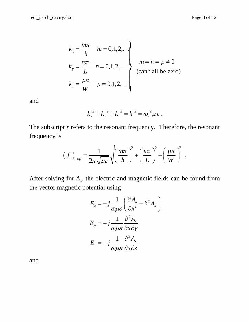
The subscript r refers to the resonant frequency. Therefore, the resonant

frequency is

2 2 2

1

2r mnp

m n pf

h L W

.

After solving for Ax, the electric and magnetic fields can be found from

the vector magnetic potential using

2

2

2

2

1

1

1

xx x

xy

xz

AE j k A

x

AE j

x y

AE j

x z

and


0 (transverse magnetic)

1

1

x

xy

xz

H

AH

z

AH

y

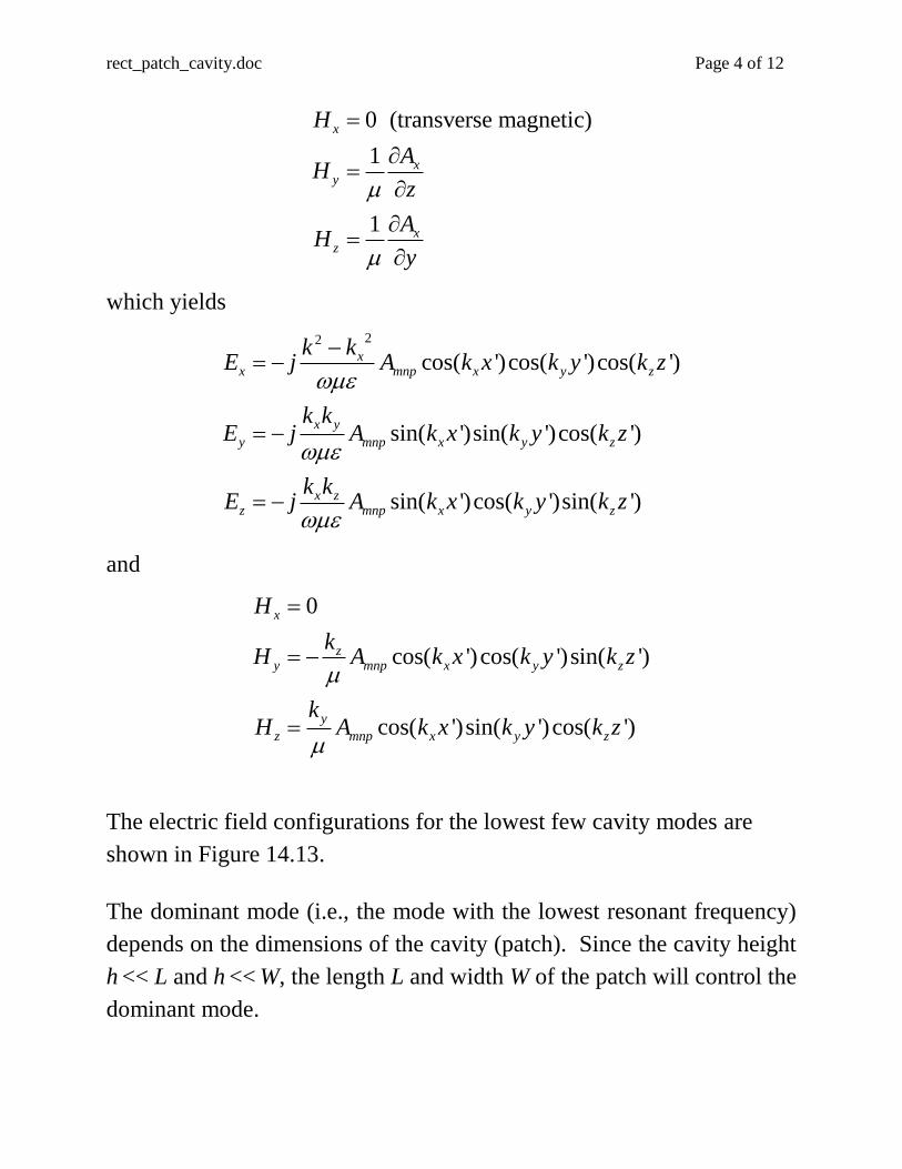
which yields

22

cos( ')cos( ')cos( ')

sin( ')sin( ')cos( ')

sin( ')cos( ')sin( ')

xx mnp x y z

x y

y mnp x y z

x zz mnp x y z

k kE j A k x k y k z



and

0

cos( ')cos( ')sin( ')

cos( ')sin( ')cos( ')

x

zy mnp x y z

y

z mnp x y z

H

kH A k x k y k z

kH A k x k y k z

The electric field configurations for the lowest few cavity modes are

shown in Figure 14.13.

The dominant mode (i.e., the mode with the lowest resonant frequency)

depends on the dimensions of the cavity (patch). Since the cavity height

h << L and h << W, the length L and width W of the patch will control the

dominant mode.


Figure 14.16 Field configurations (modes) for rectangular microstrip

patch. [From Balanis, Antenna Theory, Analysis and Design (Fourth Edition)]

If L > W > h, the dominant mode (i.e., the desired mode) is the TMx

010

where the resonant frequency is

010

1

2 2r

r

cf

L L .

Further, if L > W > L/2 > h, the next highest mode (after TMx010) is the

TMx001

001

1

2 2r

r

cf

W W .


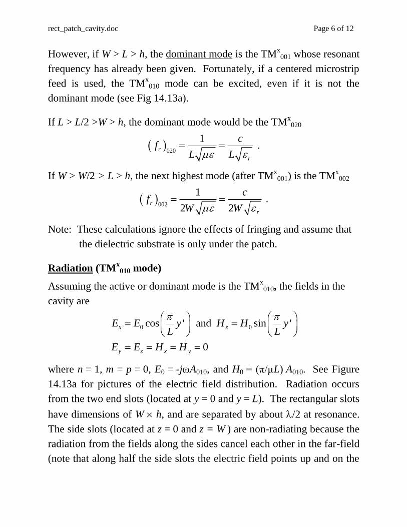
However, if W > L > h, the dominant mode is the TMx001 whose resonant

frequency has already been given. Fortunately, if a centered microstrip

feed is used, the TMx010 mode can be excited, even if it is not the

dominant mode (see Fig 14.13a).

If L > L/2 >W > h, the dominant mode would be the TMx020

020

1r

r

cf

L L .

If W > W/2 > L > h, the next highest mode (after TMx001) is the TM

x002

002

1

2 2r

r

cf

W W .

Note: These calculations ignore the effects of fringing and assume that

the dielectric substrate is only under the patch.

Radiation (TM

x010 mode)

Assuming the active or dominant mode is the TMx010, the fields in the

cavity are

0 0cos ' and sin '

0

x z

y z x y

E E y H H yL L

E E H H

where n =

1, m

=

p

=

0, E0

= -jA010, and H0

= (π/µL) A010. See Figure

14.13a for pictures of the electric field distribution. Radiation occurs

from the two end slots (located at y =

0 and y

=

L). The rectangular slots

have dimensions of W h, and are separated by about /2 at resonance.

The side slots (located at z =

0 and z = W ) are non-radiating because the

radiation from the fields along the sides cancel each other in the far-field

(note that along half the side slots the electric field points up and on the


other half it points down).

The far-field radiated electric fields radiated by each slot (see Chapter

12) are

0

0 0

0

sin( ) sin( )sin

2

r

jk r

E E

k hW E e X ZE j

r X Z

where and are the standard spherical coordinate angles, and

0

0

sin cos2

cos2

k hX

k WZ

.

If k0 h << 1, then E reduces to

0 00 sin cos

2sin

cos

jk r k WhE e

E jr

Note, the voltage across the slot is V0=h E0.

Modeling the radiating slots as a two-element array (see Chapter 6) of

rectangular aperture antennas leads to

0tot 0 0 0 eff

0

sin( ) sin( )sin cos sin sin

2

r

jk r

E E

k hW E e k LX ZE j

r X Z

Again, if k0 h << 1, this reduces to

0 0tot 0 0 eff2 sin cos

cos sin sin2sin 2

cos

jk r k WhE e k L

E jr

Note, the voltage across the slot is V0 = h E0 .


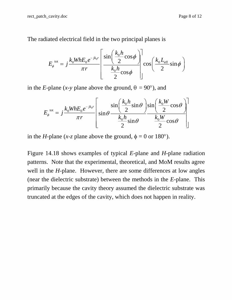
The radiated electrical field in the two principal planes is

0

0

tot 0 0 0 eff

0

sin cos2 cos sin

2cos

2

jk r

k h

k WhE e k LE j

k hr

in the E-plane (x-y plane above the ground, = 90), and

0

0 0

tot 0 0

0 0

sin sin sin cos2 2

sin

sin cos2 2

jk r

k h k W

k WhE eE j

k h k Wr

in the H-plane (x-z plane above the ground, = 0 or 180).

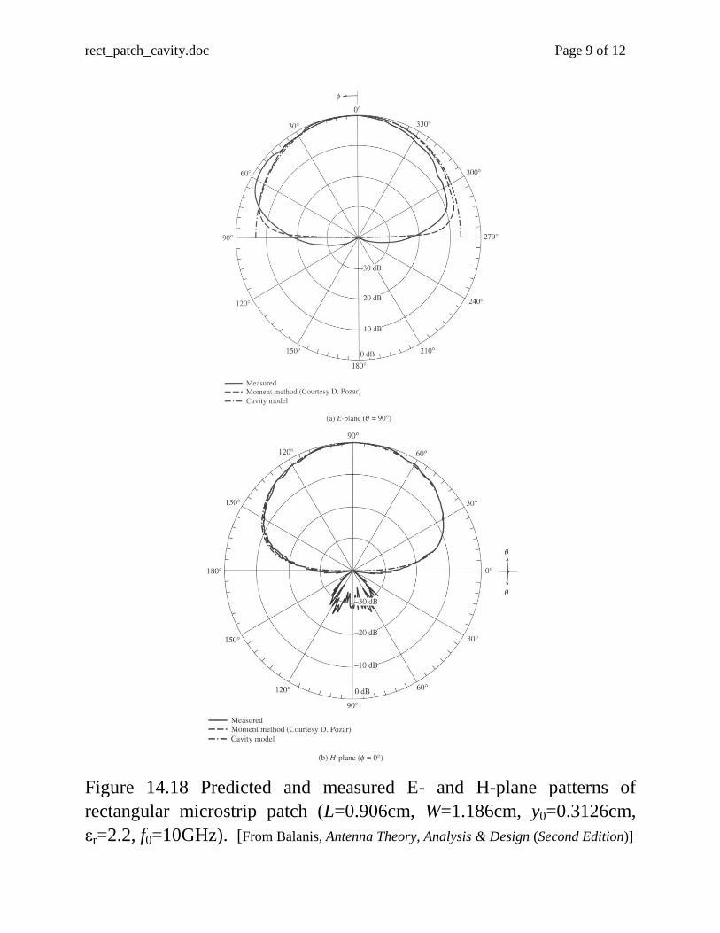
Figure 14.18 shows examples of typical E-plane and H-plane radiation

patterns. Note that the experimental, theoretical, and MoM results agree

well in the H-plane. However, there are some differences at low angles

(near the dielectric substrate) between the methods in the E-plane. This

primarily because the cavity theory assumed the dielectric substrate was

truncated at the edges of the cavity, which does not happen in reality.


Figure 14.18 Predicted and measured E- and H-plane patterns of

rectangular microstrip patch (L=0.906cm, W=1.186cm, y0=0.3126cm,

εr=2.2, f0=10GHz). [From Balanis, Antenna Theory, Analysis & Design (Second Edition)]


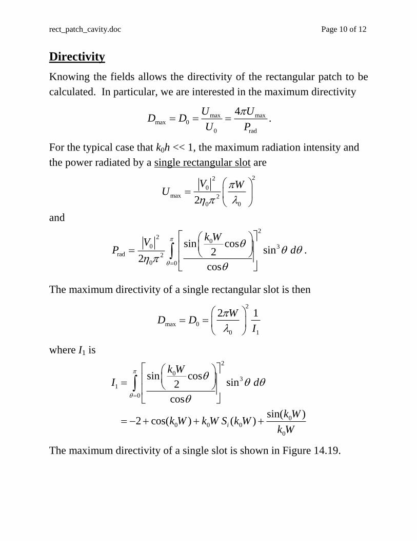
Directivity

Knowing the fields allows the directivity of the rectangular patch to be

calculated. In particular, we are interested in the maximum directivity

max maxmax 0

0 rad

4U UD D

U P

.

For the typical case that k0h << 1, the maximum radiation intensity and

the power radiated by a single rectangular slot are

22

0

max 2

0 02

V WU

and 2

20

0 3

rad 2

0 0

sin cossin2

2cos

k WV

P d

.

The maximum directivity of a single rectangular slot is then

2

max 0

0 1

2 1WD D

I

where I1 is 2

03

1

0

00 0 0

0

sin cossin2

cos

sin( )2 cos( ) ( )i

k W

I d

k Wk W k W S k W

k W

The maximum directivity of a single slot is shown in Figure 14.19.


The maximum directivity of a rectangular patch (2 radiating slots) is

2

tot tot

max 0

0 2 rad 0

2 2

15

W WD D

I G

where Grad is the radiation conductance and

2

03 2 0 eff

2

0 0

sin cossin cos sin sin2

2cos

k Wk L

I d d

.

A slightly simpler expression for the maximum directivity is

tot tot

max 0 0

12 1

2

1 /D D D

G G

.

The directivities for two slots (i.e., rectangular patch) are shown in

Figures 14.19 and 14.20 as functions of slot width W and substrate

height h.

The HPBWs in the E-plane and H-planes are (very) approximately

21 0

2 2 2

eff

7.032sin (14-58)

4 3E

L h

and

1

0

12sin (14-59)

2H

k W

.


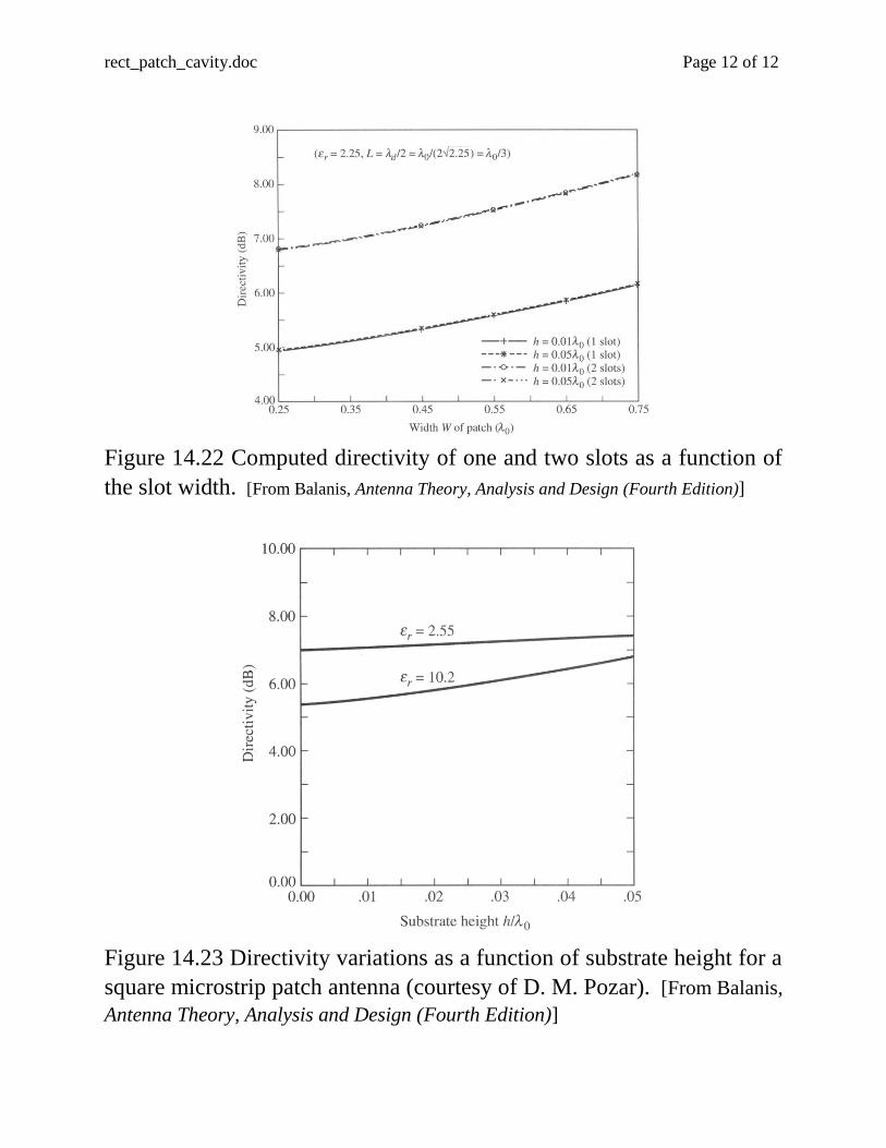
Figure 14.22 Computed directivity of one and two slots as a function of

the slot width. [From Balanis, Antenna Theory, Analysis and Design (Fourth Edition)]

Figure 14.23 Directivity variations as a function of substrate height for a

square microstrip patch antenna (courtesy of D. M. Pozar). [From Balanis,

Antenna Theory, Analysis and Design (Fourth Edition)]

Microstrip Antennas Rectangular Patch - Dr. Montoya's...

Documents

Transcript of Microstrip Antennas Rectangular Patch - Dr. Montoya's...