Microsoft Excel 2016 - ucc.ie · Excel 2016 UCC Computer Training Centre ii Email [email protected]...

IT Training Centre University College Cork

Email [email protected]

Excel 2016

Level 2

Excel 2016

UCC Computer Training Centre i Email [email protected]

TABLE OF CONTENTS

What’s New in Excel 2016? _______________________________ 1

Protected View __________________________________________________ 1

Where to Save your Files ________________________________ 2

Design Considerations when creating an excel spreadsheet______ 3

Customize the Layout ____________________________________________ 3 Split a Worksheet ______________________________________________ 3 Freeze Rows and Columns _______________________________________ 4 Repeat rows on the Printed Page __________________________________ 4

Formula & Functions ____________________________________ 5 Precedence of Operators ________________________________________ 5 To create a basic formula in Excel: ________________________________ 6

Functions ____________________________________________ 6 Elements of a Function _________________________________________ 6

AutoSum _____________________________________________ 7 Using the Average, Count, Max and Min Functions ____________________ 7 Function Library _______________________________________________ 7 To calculate a function: _________________________________________ 8

Names ______________________________________________ 9 The scope of a name ___________________________________________ 9 To define a name ______________________________________________ 9 Manage names by using the Name Manager dialogue box _____________ 10

Cell Referencing ______________________________________ 11 Relative Cell Reference ________________________________________ 11 Absolute Cell Reference ________________________________________ 11 Mixed Cell References _________________________________________ 12

Sorting Data _________________________________________ 13

AutoFilter ___________________________________________ 14 Create criteria _______________________________________________ 14 To remove criteria ____________________________________________ 15 To turn off the AutoFilter _______________________________________ 15

Advanced Filter _______________________________________ 16 One condition in two or more columns ____________________________ 16 One condition in one column or another ___________________________ 16 One of two sets of conditions for two columns ______________________ 16 More than two sets of conditions for one column ____________________ 17 To turn off the Advanced Filter __________________________________ 17 Filtering Exercises ____________________________________________ 18

Conditional Formatting _________________________________ 19

To Clear Rules _________________________________________________ 19

Using Format as a Table ________________________________ 20

Sparklines ___________________________________________ 20

Subtotals ___________________________________________ 21 Displaying Subtotals __________________________________________ 21 To replace existing subtotals ____________________________________ 23

Excel 2016

UCC Computer Training Centre ii Email [email protected]

To add further subtotals without removing existing ones ______________ 23 Removing Subtotals ___________________________________________ 23

IF Function __________________________________________ 24 Nested Functions _____________________________________________ 25

Useful functions for General Use _________________________ 26

Managing Worksheets within a Workbook __________________ 27 Sheet Tab ___________________________________________________ 27 Insert a Worksheet ___________________________________________ 27 Renaming a Worksheet ________________________________________ 27 Changing the Tab Colour of a Worksheet __________________________ 28 Deleting a Worksheet __________________________________________ 28 Moving Worksheets within a Workbook ____________________________ 28 Copying Worksheets within a Workbook ___________________________ 28 Copying or Moving Worksheets to Other Workbooks __________________ 28 To hide a worksheet ___________________________________________ 29 To unhide a worksheet _________________________________________ 29

Collating Data from Several Worksheets ___________________ 30 Formulas – using cells from different worksheets ____________________ 31 Functions – using cells from different worksheets ____________________ 31

Charts ______________________________________________ 31 Creating a Chart ______________________________________________ 32 Chart Tools __________________________________________________ 32 Modifying Chart Data __________________________________________ 33 Deleting a Data Series _________________________________________ 33 Adding a Data Series __________________________________________ 33 Resizing a Chart ______________________________________________ 33 Deleting a Chart ______________________________________________ 33

Pivot Tables _________________________________________ 34

Changing the Value Field Settings __________________________________ 36

Refreshing the Data _____________________________________________ 36

Pivot Charts _________________________________________ 37

Quick Analysis Tool ____________________________________ 38

Hide or display the Paste Options button ___________________ 40

Using Paste Special ____________________________________ 40

Object Linking and Embedding (OLE Linking) ________________ 41

Embedding an Excel Worksheet in Word _____________________________ 41 To Edit an Embedded Worksheet in Word __________________________ 41

To Link an Excel Worksheet in Word ________________________________ 42 To Edit a Linked Worksheet in Word ______________________________ 42 To break a Linked Worksheet in Word _____________________________ 43

Protecting Your Work __________________________________ 44

Applying Password Protection to a File ______________________________ 44 Applying a Modification Password ________________________________ 45 Setting the Read-Only Recommended Option _______________________ 45

Protecting Data within the Workbook _______________________________ 45 Protect an Individual Worksheet _________________________________ 46

Excel 2016

UCC Computer Training Centre iii Email [email protected]

Remove protection from an individual worksheet ____________________ 46 Specify which cells can be changed after a worksheet is protected ______ 46

Hiding Sheets and Cells __________________________________________ 47 Hiding a Worksheet ___________________________________________ 47 Unhiding a Worksheet _________________________________________ 47 Hiding Rows _________________________________________________ 47

Cell Comments _______________________________________ 48 Add a comment to a cell _______________________________________ 48 Edit a comment ______________________________________________ 48 Delete a comment ____________________________________________ 48 Print a worksheet with comments ________________________________ 49

Data Validation _______________________________________ 50

Importing Data using the Text Import Wizard _______________ 51

Keyboard Shortcuts ___________________________________ 53

Notes ______________________________________________ 54

Excel 2016

UCC Computer Training Centre 1 Email [email protected]

What’s New in Excel 2016?

Excel 2016 is designed to help you get professional-looking results quickly. New

features include:

• Tell Me What you want to do

• Pivot Table & Pivot Chart enhancements – Search field, Date grouping

• Six new Chart Types

• 3D Data map

• Power Query – this was previously an Add-in

• Data Forecasting

Protected View Files from the Internet and from other potentially unsafe locations can contain

viruses, worms, or other kinds of malware, which can harm your computer. To

help protect your computer, files from these potentially unsafe locations are

opened in Protected View. By using Protected View, you can read a file and

inspect its contents while reducing the risks that can occur.

There are several reasons why a file opens in Protected View including;

• The file was opened from an Internet location

• The file was received as an Outlook 2016 attachment and your computer

policy has defined the sender as unsafe

• The file was opened from an unsafe location. An example of an unsafe

location is your Temporary Internet Files folder.

Note: System administrators can extend the list of potentially unsafe

locations to include additional folders also considered unsafe.

If you know the file is from a trustworthy source, and you want to edit, save, or

print the file, then you can exit Protected View by clicking Enable Editing on the

Message Bar. After you leave Protected View, it becomes a trusted document.

Excel 2016


Where to Save your Files

When saving work related UCC files use one of the following options:

• NAS – this is the UCC network. Files stored on nas are backed up daily.

Select this PC and navigate to nas. Folders can be setup to allow multiply

users access to files. Check with your system administrator where on nas

you have access to.

• One Drive - University College Cork – this is One Drive for Business

which is web-based storage. Saving here means you will have access to

the file anywhere on any device once you are connected to the internet.

This is generally used for a user’s individual work files and for short-term

sharing and collaboration.

• Sites – University College Cork – SharePoint which is a web-based

document management system. Saving here means you will have access

to the file anywhere on any device once you are connected to the internet.

This is generally used for project-based files where a group of users need

to share and collaborate on files. The SharePoint site would need to be set

up in advance, check with your system administrator.

Note: Work related files should NOT be stored long-term on your PC (in the

Documents folder, for example). If files are stored here the onus is on the

user to back-up regularly.

One Drive Personal is NOT recommended for work files.

Excel 2016


Design Considerations when creating an excel

spreadsheet

A good design enables you to maximise utilisation of many of the automatic

features for managing and analysing data e.g. sorting, subtotals, filters, pivot

tables, functions etc.

The following are some of the basic guidelines to remember when setting up your

spreadsheet:

▪ Column headings should be short (using some of the Text Control features

within Format Cells, Home tab may help).

▪ Each column heading should be unique.

▪ Apply some type of different formatting (e.g. make the text bold or apply a

background colour) to the cells containing the column headings.

▪ Avoid blank rows or columns in the block of data.

▪ Column content should be of the same data type.

▪ Have only 1 list per worksheet, however, if additional lists are required on

the same sheet, position diagonally below & to the right of the other list.

▪ Ctrl Home goes to cell A1

The Excel 2016 worksheet holds large amounts of data. A single worksheet now

consists of 1,048,576 rows and 16,384 columns, which means you have more

than 17 billion cells in which you can enter data and perform calculations.

Customize the Layout

Split a Worksheet You can split a worksheet into multiple resizable panes for easier viewing of parts

of a worksheet. To split a worksheet:

▪ Select any cell in centre of the worksheet you want to split

▪ Click the Split button on the View tab

▪ Notice the split in the screen, you can manipulate each part separately

Excel 2016


Freeze Rows and Columns

You can select a particular portion of a worksheet to stay static while you work on

other parts of the sheet. This is accomplished through the Freeze Rows and

Columns Function. To Freeze a row or column:

▪ Click the Freeze Panes button on the

View tab

▪ Either select a section to be frozen or click

the defaults of top row or left column

▪ To unfreeze, click the Freeze Panes

button

▪ Click Unfreeze

Repeat rows on the Printed Page

Freeze panes keep certain rows or columns visible regardless of your location on

a spreadsheet. On the printed page it can to useful to have the same column and

rows visible on all pages. To do this you must setup the spread sheet to print

titles

▪ On the Page Layout Tab

▪ In the Page Setup group

▪ Click the Print Titles button

▪ The Sheet tab of the page setup dialog box

will open

▪ In the Print Title area use the selection

button to select the Rows you want repeated

at the top of each page and then the other

selection button to choose the columns you

want repeated on the left of each printed

page.

Excel 2016


Formula & Functions

Precedence of Operators

The term precedence refers to the order in which Excel performs calculations in a

formula. Excel follows these rules:

▪ Expressions within parentheses are processed first.

▪ Multiplication and division are performed before addition and subtraction

▪ Consecutive operations with the same level of precedence are calculated

from left to right.

See below for examples of how these rules apply, remembering that normally

when using excel for formulas, the formulas would contain cell references instead

of actual values.

Formula Precedence of the calculations Result

=1+2*3 2*3 is calculated first = 6 then 1 is

added

7

=(1+2)*3 1+2 is calculated first = 3 then this

answer is multiplied by 3

9

=3*6+12/4-2 3*6 is calculated = 18

18+12/4-2, then 12 is divided by 4

18+3-2

19

=(3*6)+12/(4-2) 3*6 is calculated = 18

18+12/(4-2) then 2 is deducted from 4

18+12/2, then 12 is divided by 2

18+6

24

Excel Formulas

A formula is a set of mathematical instructions that can be used in Excel to

perform calculations. Formals are started in the formula box with an = sign.

There are many elements to and excel formula.

References: The cell or range of cells that you want to use in your calculation

Operators: Symbols (+, -, *, /, etc.) that specify the calculation to be

performed

Constants: Numbers or text values that do not change

Functions: Predefined formulas in Excel

Excel 2016


To create a basic formula in Excel:

▪ Position the cell pointer in the cell that will contain the result of the formula.

▪ Type an = equal sign.

▪ Click with the mouse on the cell to be calculated.

▪ Type the mathematically operator to be used in the formula.

▪ Click on the next cell to be calculated.

▪ Click Enter to return the result of the formula or click on

the tick on the formula bar. The result of the formula is

displayed in the worksheet cell. The actual formula controlling the result

will be displayed in the formula bar of the worksheet.

Functions

A function is a built in formula in Excel. A function has a name and arguments

(the mathematical function) in parentheses.

Elements of a Function

The following elements are common in all functions:

= must start with an equal sign

function name must have a name

(….) must have arguments enclosed in brackets;

there are a few exceptions e.g =now( )

Commonly used functions in Excel include:

Sum: Adds a range of cells

Average: Calculates the average of a range of cells

Min: Finds the minimum value of a range of cells

Max: Finds the maximum value of a range of cells

Count: Finds the number of cells that contain a numerical value within a

range of cells.

Excel 2016


AutoSum

The SUM function is the most commonly used function so to

make it more accessible there is an AutoSum button on the

Home tab.

▪ Position the cell pointer in the cell that will contain the result of the function.

▪ Click on the AutoSum button

Excel will guess the range of cells to be calculated and it will insert the

=SUM function. If the range of cells is not correct use the mouse to select

the correct range of cells to be added.

(use the mouse and the Ctrl key to select non-adjacent cells)

▪ Press return to display the results in the cell or click on the tick on the

formula bar.

Using the Average, Count, Max and Min Functions

▪ Click on the down arrow to the right of the AutoSum

button and select the required function e.g. Average

▪ Excel will guess the range of cells to be calculated and it

will insert the =Average function. If the range of cells is

not correct use the mouse to select the correct range of

cells to be included in the calculation.

▪ Press return to display the results in the cell or click on

the tick on the formula bar.

Function Library

The function library is a large group of functions on the Formula Tab of the

Ribbon. These functions include:

Recently Used: All recently used functions

Financial: Accrued interest, cash flow return rates and additional financial

functions

Logical: And, If, True, False, etc.

Text: Text based functions

Date & Time: Functions calculated on date and time

Math & Trig: Mathematical Functions

Excel 2016


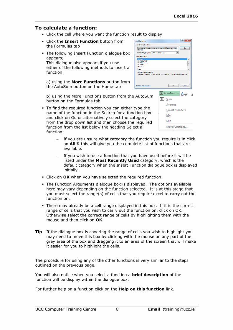
To calculate a function:

▪ Click the cell where you want the function result to display

▪ Click the Insert Function button from

the Formulas tab

▪ The following Insert Function dialogue box

appears;

This dialogue also appears if you use

either of the following methods to insert a

function:

a) using the More Functions button from

the AutoSum button on the Home tab

b) using the More Functions button from the AutoSum

button on the Formulas tab

▪ To find the required function you can either type the

name of the function in the Search for a function box

and click on Go or alternatively select the category

from the drop down list and then choose the required

function from the list below the heading Select a

function:

− If you are unsure what category the function you require is in click

on All & this will give you the complete list of functions that are

available.

− If you wish to use a function that you have used before it will be

listed under the Most Recently Used category, which is the

default category when the Insert Function dialogue box is displayed

initially.

▪ Click on OK when you have selected the required function.

▪ The Function Arguments dialogue box is displayed. The options available

here may vary depending on the function selected. It is at this stage that

you must select the range(s) of cells that you require excel to carry out the

function on.

▪ There may already be a cell range displayed in this box. If it is the correct

range of cells that you wish to carry out the function on, click on OK.

Otherwise select the correct range of cells by highlighting them with the

mouse and then click on OK.

Tip If the dialogue box is covering the range of cells you wish to highlight you

may need to move this box by clicking with the mouse on any part of the

grey area of the box and dragging it to an area of the screen that will make

it easier for you to highlight the cells.

The procedure for using any of the other functions is very similar to the steps

outlined on the previous page.

You will also notice when you select a function a brief description of the

function will be display within the dialogue box.

For further help on a function click on the Help on this function link.

Excel 2016


Names

A name is a description that you assign to a cell or group of cells. Names are an

alternative to cell references. Once a name has been defined, you can refer to it

in a formula; for example, =sum(Year1). You can use names to move quickly to a

certain area of the workbook or to specify print ranges.

The scope of a name

All names have a scope, either to a specific worksheet (also called the local

worksheet level) or to the entire workbook (also called the global workbook

level). The scope of a name is the location within which the name is recognized

without qualification. For example:

▪ If you have defined a name, such as Budget_FY08, and its scope is Sheet1,

that name, if not qualified, is recognized only in Sheet1, but not in other

sheets without qualification.

▪ To use a local worksheet name in another worksheet, you can qualify it by

preceding it with the worksheet name, as the following example shows:

▪ Sheet1!Budget_FY08

▪ If you have defined a name, such as Sales_Dept_Goals, and its scope is the

workbook, that name is recognized for all worksheets in that workbook, but

not for any other workbook.

To define a name

▪ Select the cell or range of cells.

▪ Click in the Name Box

(the name box is located to the left of the

formula bar and normally contains the cell

reference of the active cell)

▪ Type the name and press enter. A name cannot contain spaces and the first

character must be text or an underscore character.

▪ By default, names use absolute cell references (absolute cell reference: In a

formula, the exact address of a cell, regardless of the position of the cell

that contains the formula. An absolute cell reference takes the form $A$1.).

Define Name dialogue box may also be used to refer to a value instead of a

cell range e.g. you may have a formula =B2*Bonus where Bonus is a value

defined not a cell/cell range containing that value.

Excel 2016


Manage names by using the Name Manager dialogue box

• Use the Name Manager dialogue box to

work with all of the defined names in the

workbook.

• For example, you may want to find

names with errors, confirm the value and

reference of a name, view or edit

descriptive comments, or determine the scope. You can also sort and filter

the list of names, and easily add, change, or delete names from one

location.

• To open the Name Manager dialogue box, on the Formulas tab, in the

Defined Names group, click Name Manager.

Excel 2016


Cell Referencing

There are three types of cell addressing used in Excel – relative, absolute and

mixed. The following examples will explain the difference between them. The

choice of addressing mode becomes significant when a formula is either moved or

copied to a new location.

Relative Cell Reference

Relative addressing is the most commonly used type of addressing. It assumes

that the relative relationship will be the same if a formula is copied from one cell

to another.

In this example above the formula in cell E7 calculates Alan Doyle’s tax liability

i.e. Gross Pay multiplied by Tax Rate. This formula uses the most common type

of cell addressing which is relative addressing. However, in this case it would

cause errors if copied to the cells underneath. This is because the tax rate is

referenced in cell B3 and this would change to B4, B5, and B6 and so on as the

formula is copied down the column.

Absolute Cell Reference

The figure below shows how absolute cell addressing will solve this problem. To

copy the formula in this case, you need to use absolute addressing to lock the cell

reference, B3. To create an absolute address, a dollar sign ($) is placed in front of

the column and row reference, e.g. B3 becomes $B$3. Once absolute addressing

is used, the cell reference will remain the same regardless of where it is copied to

on the worksheet.

Relative Cell Referencing

If the formula in this cell is

copied to cells E8 and E9

underneath it, the formula will

change to:

=D8*B4 (in cell E8)

=D9*B5 (in cell E9)

These formulas would cause

errors as the Tax Rate is

contained in cell B3 and this

reference should remain

constant.

Absolute Cell

Referencing:

A dollar sign $ is placed

in front of the column and

row reference. Now when

the formula is copied to

cells E8 and E9, it will

copy as:

=D8*$B$3 (in cell E8)

=D9*$B$3 (in cell E9)

Excel 2016


Mixed Cell References

Cell C5 contains the formula C$4*$B5

Firstly consider the cell reference C$4 – column C is relative but row 4 is

absolute. When this is auto-filled down to C6 you will notice that the cell

reference doesn’t change, however when it is auto-filled to the right the column

reference will change from C to D to E.

Now consider the cell reference $B5 - column B is absolute but row 5 is relative.

When this is auto-filled down to C6 you will notice that the row reference changes

but when it is auto-filled to the right there is no change in the column reference.

This is an example of where you may use both types of Mixed Cell Referencing

Tip you can adjust references in a formula by placing the insertion point any-

where adjacent to the reference and pressing the function key F4 on the

keyboard. Each time you press F4 the cell reference will toggle between

absolute, mixed or relative cell references.

Mixed Cell Referencing

C$4 – column C is

relative but row 4 is

absolute

$B5 – column B is

absolute but row 5 is

relative

Excel 2016


Sorting Data

You use the Sort command to arrange the rows of a data list alphabetically or

numerically in ascending or descending order, based on the contents of the fields,

or columns.

Ascending will sort the lowest number, the beginning of the

alphabet, or the earliest date first in the sorted range.

Descending will sort the highest number, the end of the alphabet,

or the latest date first in the sorted range. Blank cells are always

sorted last.

▪ Click into a cell within the column you wish to sort.

▪ Click on the Home Tab and then click the down arrow to

right of the Sort & Filter command button located to the right of the screen

within the Editing group.

For more detailed sorting select Custom Sort or from the Data Tab click o the

Sort command.

Office Excel 2016 allows the user to involve up to 64 criteria in one sort.

In Excel 2016 you can also sort by Values, Cell Colour, Font Colour or Cell Icon

(Conditional Formatting).

▪ On the Data tab, in the Sort & Filter group, click Sort to display the Sort

dialog box shown. Because row 6 contains headings for our data columns,

we check the My Data Has Headers box. We will now select the following

four criteria in the order shown:

▪ Sort by the Surname column so that Values (this means cell contents) are

in A to Z order.

▪ Sort by the Forename column so that Values are in A to Z order.

▪ Click the Add Level button twice to give a total; of four levels

▪ Sort by the Gross Pay column so that Values are in order from largest to

smallest.

▪ Sort by the Tax column so that Values are in order from largest to smallest.

Excel 2016


AutoFilter

The AutoFilter feature puts drop-down arrows (with menus) in the titles of each

column. The menus are used to select criteria in the column

so that only records that meet the specified criteria are

displayed.

▪ Select a cell within the list.

▪ On the Home tab, in the Editing group, click Sort &

Filter, and then click on the Filter command.

An arrow appears to the right of each column label.

▪ Example: To display only the people in the MIS

department, remove the arrow next to Select All,

and select MIS from the list.

To display all the names in the list again, select the

Department drop down arrow, and Clear Filter from

“Department”.

Create criteria

▪ Point to Text Filters and then click one of the

comparison operators or click Custom Filter.

▪ For example, to filter by text that begins with a

specific character, select Begins With, or to filter by

text that has specific characters anywhere in the text,

select Contains.

▪ In the Custom AutoFilter dialog box, in the box on the

right, enter text or select the text value from the list.

Optionally, filter by one more criteria.

How to add one or more criteria

▪ To filter the table column or selection so that both criteria must be true,

select And.

▪ To filter the table column or selection so that either or both criteria can be

true, select Or.

▪ In the second entry, select a comparison operator, and then in the box on

the right, enter text or select a text value from the list.

Excel 2016


Example:To display a list of Employees whose Tax liability is less than 3,500

▪ From the Tax Column, select Number Filters and

select Custom Filter.

▪ In the Custom AutoFilter dialog box, select the

“is less than” option by clicking on the arrow

under Tax to display the drop-down list.

▪ Type 3500 and click OK. Ten records match the

criteria.

▪ To show all records again, select the Tax drop

down arrow, and Clear Filter from “Tax”.

To remove criteria

• Click anywhere with the filtered list

• On the Data Tab in the Sort & Filter group click on the

Clear button.

• The full list will be displayed again but the filter dropdown arrows are still

available

To turn off the AutoFilter

▪ On the Home tab, in the Editing group, click Sort & Filter, and then

deselect Filter.

Excel 2016


Advanced Filter

The AutoFilter command on the Home Tab is usually the quickest way to filter a

list. However, if you want to filter a list using multiple sets of criteria or criteria

containing formulas use the Advanced Filter command on the Data Tab.

The Advanced Filter enables you to filter data by using a criteria range to display

only the rows that meet all the criteria you specify.

One condition in two or more columns

To find data that meets one condition in two or more columns, enter all the

criteria in the same row of the criteria range.

One condition in one column or another

To find data that meets either a condition in one column or a condition in another

column, enter the criteria in different rows of the criteria range.

One of two sets of conditions for two columns

To find rows that meet one of two sets of conditions, where each set includes

conditions for more than one column, type the criteria in separate rows.

.

e.g. this criteria range displays all rows that contain "Accounts" in the

Department column, with a tax value greater than €3,200 in the Tax

column, and Net Pay less than €8,000.

e.g. this criteria range displays all rows that

contain either "Accounts" in the

Department column, “Forde” in the

Surname column or “Alan” in the

Forename column.

+e.g. this criteria range displays the rows that contain both "Accounts" in

the Department column and Gross Pay greater than or equal to

€13,000, and also displays the rows for Personnel Department with Gross

Pay greater than €12,000

Excel 2016


More than two sets of conditions for one column

To find rows that meet greater than two sets of conditions, include multiple

columns with the same column heading.

As an example, we will extract from the list all Employees whose Gross Pay is

greater than €14,000 from the Personnel Department and also employees from

the Marketing Department with a Gross Pay greater than €13,000

▪ Insert several blank rows at the very top of your worksheet. (Your column

headings should now be on row 10 of the worksheet)

▪ Select the column headings in Row 10 and copy. Paste the headings into

Row 1 of the worksheet.

▪ Enter the criteria for the advanced filter as follows;

▪ Click into any cell within the list and then select the Data tab. In the Sort &

Filter group choose Advanced Filter…

▪ Ensure that the List Range is $A$11:$G$29

▪ The Criteria Range - specifies the range of cells on

your worksheet that contains your criteria. In this

example it should be $A$1:$G$3, to ensure this

click into the Criteria range box and then with the

mouse click into cell A1 of the worksheet and

highlight to cell G3.

▪ Under the heading Action there are 2 options:

Filter the list, in-place - hides the rows that do not

meet the criteria and the filtered list is displayed

where the existing List range had been displayed.

Copy to Another Location copies the filtered data to another worksheet or

another location on the same worksheet. If this option is selected the Copy

to: box will no longer be greyed out and you click into this box and select

where you wish the filtered list to appear.

▪ Click OK. This will return you to the worksheet, and display the records that

match the criteria.(Three records meet the criteria)

To turn off the Advanced Filter

From the Data tab in the Sort & Filter Group click on

Clear.

e.g. this criteria range displays Gross Pay that

are between €14,000 and €15,000 in

addition to Gross Pay that are less than

€12,000.

Excel 2016


Filtering Exercises

Use the AutoFilter to solve the following:

1. Search for Employees with Net Pay greater than €8000 and who are in

the Accounts Department.

Two records match the criteria – Mary Forde and Elizabeth Murphy.

2. Search for Employees with Tax greater than €3000 and whose Net Pay is

greater than €9000.

Two records match the criteria

3. Search for Employees who are in either the Accounts or Personnel

departments. Eight records match the criteria

Use the Advanced Filter to solve the following:

1. Search for Employees working in the Personnel Department, with a Net

Pay that is less than €7,500 and employees working in the Admin

Department, with a Net Pay of more than €7,500. Filter the list in

place.

Four records match the criteria.

2. Search for Employees working in the Accounts Department, paying more

than €3,500 Tax and employees working in the Marketing Department,

with a Pension of less than €1,300. Copy the filter results to cell J2.

Three records match the criteria.

Excel 2016


Conditional Formatting

Conditional formatting helps make it easy to highlight interesting cells or ranges

of cells, emphasize unusual values, and visualize data by using data bars,

color scales, and icon sets. A conditional format changes the appearance

of a cell range based on a condition (or criteria). If the condition is true,

the cell range is formatted based on that condition; if the conditional is

false, the cell range is not formatted based on that condition.

Note: When you create a conditional format, you can only

reference other cells on the same worksheet; you cannot reference

cells on other worksheets in the same workbook, or use external

references to another workbook.

▪ Select one or more cells in a range.

▪ On the Home tab, in the Styles group, click the arrow next to

Conditional Formatting, and then click Colour Scales, Icon

Sets or Data Bars

▪ To manage the rules for any of these types of formatting

choose More Rules..within the type selected

▪ The New Formatting Rule dialog box appears

This allows you to

− Format all cells based on their values

− Format only cells that contain

− Format only top or bottom ranked values

− Format only values that are above or below

average

− Format only unique or duplicate values

− Use a formula to determine which cells to

format

• The Format style chosen e.g 2/3 colour scale or

Data Bars etc will determine how the criteria for

the Conditional Formatting can be edited.

To Clear Rules ▪ Select the cells you wish to remove the conditional formatting from

▪ Click on the arrow to the right of the Conditional Formatting command and

select Clear Rules.and then Clear from Selected Cells.

▪ Alternatively you may wish to remove all conditional formatting by selecting

Clear Rules from Entire Sheet.

Excel 2016


Using Format as a Table

The Format as Table may also contain a style that suits the

data.

• Select the Cells you want wish to format

• In the Styles Group on the Home Tab

• Click on the Format as a Table button and choose a

format

• Select one of the predetermined formats.

• After clicking one of the formats, Excel will ask you what range of cells you

want to convert to a table (see figure 4). If your table contains a heading

row, make sure the checkbox is checked. Click OK to convert the range to

a table.

If you later decide that you’d prefer your data in its original form (i.e. not in a

table), you can convert it back to a range of cells.

• Click anywhere in the table and then on the Table Tools tab, on the

Design table, under the Tools group click on the Convert To Range

button.

• Once the data is converted back to a range, the table features are no

longer available.

Note: that the formatting that was applied to the table is still present and will

need to be manually re-formatted.

Sparklines

Sparklines are tiny, word-sized charts that can appear in a cell. Excel 2016 makes

it easy to create sparklines

• To locate the Sparklines option, go to the Insert tab, the Sparklines group

is here.

Note: This feature is only available since Excel 2013 so will be greyed out if you

are using a workbook that was created in an older version of Excel (Save the file

as 2016 workbook to avail of the feature).

Excel 2016


Subtotals

A long list of related items might want to be split into subgroups. Here we can

split the list into departmental groupings.

▪ Before you calculate the subtotals you must first sort the list based on the

field which you will be finding the subtotals for.

▪ Click any cell in the list.

▪ From the Data tab in the Sort & Filter group, choose Sort

▪ When the Sort dialog box appears, choose Add Level

▪ Then sort by the following

− Sort by Department

− Then by Surname

− Then by Forename

• In each case Sort On “Values” and Order A to Z

▪ Click OK.

Displaying Subtotals

▪ Click any cell in the list from the Data Tab in the

Outline group choose Subtotals

▪ Choose the following options:

- At each change in: Department

- Use function: Sum

- Add subtotal to: Net Pay

▪ The subtotals will appear below the groupings

and the Grand Total at the bottom. If you want

the subtotals and the grand total on the top

deselect the Summary below data option.

▪ Click OK

You can view the different levels of subtotals by

clicking on the appropriate level button. to

the left of the column headings or by clicking the

expand + or collapse - buttons to the left of the

row headings.

▪ To display the Grand Total – click on 1

▪ To display the Grand Total and the Subtotals – click on 2

Excel 2016


▪ To view all the data again - click on 3

Excel 2016


To replace existing subtotals

▪ Click anywhere within the existing list and then carry out the steps outlined

previously, selecting which function you wish to use and which columns you

wish to subtotal.

▪ Ensure that the Replace current subtotals check box is selected.

▪ Click on OK.

▪ The existing subtotals will be replaced with the new options that have been

select.

To add further subtotals without removing existing ones

▪ Choose Subtotals from the Data Tab in the

Outline group.

▪ Ensure that the Replace current subtotals tick

box is deselected before clicking on OK.

▪ Now you will notice that there will be 4 levels of

outline view instead of the usual 3 levels of

view.

Removing Subtotals

▪ From the Subtotals dialogue box – click on the

Remove All button.

Excel 2016


IF Function

The if function can be used for comparative analysis. It returns one value if a

condition you specify evaluates to TRUE and another if it evaluates to FALSE. Any

of the following mathematical expressions for comparison can be used:

Operator Definition

= Equal to

> Greater than

< Less than

>= Greater than or equal

to

<= Less than or equal to

<> Not equal to

If statements can be built by using the Insert Function dialogue box but it is

necessary to be familiar with the syntax of the function to be able to create

nested if functions (i.e. where you cannot resolve a problem using only TRUE and

FALSE).

Syntax

IF(logical_test,value_if_true,value_if_false)

Example

In the above example an if function is being used to return the text PASS in

column C if the student’s result in column B is 40 or more, if the result is lower

than 40 the text FAIL will be displayed in column C. The function can be typed

directly into the cell in column C, alternatively; you may wish to use the Insert

Function dialogue box to assist you, as follows:

Excel 2016


▪ Click in cell C9. From the Home tab in the Editing group

choose More Functions from the AutoSum drop down list

▪ Select the IF function from the Logical Function Category

& click on OK. The following screen is displayed:

Type C9>=40 in the Logical_test box

Type PASS in the Value_if_true box

Type FAIL in the Value_if_false box

▪ Click on OK.

Notice the structure of the function in

the formula bar. Excel has

automatically put in the required syntax for the function.

=IF(C9>=40,"Pass","Fail")

The IF function can also be used to calculate a formula either if the logical test is

true or if the logical test is false. It is also possible to combine a formula with

text/numbers, for example if the logical test is true you may wish to carry out a

formula and if it was false you may wish for a number to be displayed. See

example below

Nested Functions

You can nest a number of IF functions, as long as you don’t exceed the character

limit for single-cell entries. The formula in cell D9 is an example of a nested if

function.

=IF(B9>=85,"A",IF(B9>=70,"B",IF(B9>=55,"C",IF(B9>=40,"D","FAIL"))))

This can be typed but it is important that the syntax is correct.

Alternatively you can insert a function using the Insert function dialogue box

combined with the use of the name box.

Excel 2016


Useful functions for General Use

FUNCTION DESCRIPTION

AVERAGE returns the average (arithmetic mean) of the

arguments.

CONCATENTATE joins several text strings into one text string.

COUNT counts the number of cells that contain numbers

and numbers within the list of arguments. Use

COUNT to get the number of entries in a number

field in a range or array of numbers.

COUNTA counts all of the nonblank cells in a specified range

of cells

COUNTBLANK counts empty cells in a specified range of cells.

COUNTIF counts the number of cells within a range that meet

the given criteria.

DAYS360 returns the number of days between two dates

based on a 360day year.

(note: you can also subtract one date from another)

HLOOKUP looks for a value in the top row of a table or array of

values and returns the value in the same column

from a row you specify.

LEN returns the number of characters in a string.

LOWER converts text to lowercase.

MAX returns the largest value in a set of values.

MIN returns the smallest value in a set of values.

NOW() returns the current date and time, this is one of the

few functions that does not require any arguments.

POWER returns the result of a number to a power.

PRODUCT multiplies all the numbers given as arguments and

returns the product.

SQRT returns the square root of a number.

SUMIF adds the cells specified by a given condition or

criteria.

SUMPRODUCT multiplies corresponding numeric components in

given ranges or arrays and returns the sum of those

product.

UPPER converts text to uppercase.

VLOOKUP searches for a value in the leftmost column of a

table, and then returns a value in the same row

from a column you specify in the table.

Excel 2016


Managing Worksheets within a Workbook

The Excel 2016 "Big Grid" increases the maximum number of rows per worksheet

from 65,536 to over 1 million, and the number of columns from 256 (IV) to

16,384 (XFD). When you open a new workbook there 1 worksheet by default. In

the previous version there was 3 by default.

This default can be changed within File – Options – General

Sheet Tab

The names of the sheets appear on tabs at the bottom of the workbook window.

To move from sheet to sheet, click the sheet tabs.

Insert a Worksheet

▪ Click on the + to the right of Sheet1.

Alternatively, from the Home Tab in the Cells

Group click on Insert and select Insert Sheet.

Renaming a Worksheet

▪ Right click on the sheet tab and select Rename,

alternatively double click on the sheet tab.

▪ Type a new name for the sheet and press enter.

Double click

to rename

Click on + to

add a new

worksheet

Excel 2016


Changing the Tab Colour of a Worksheet

▪ Right click on the sheet tab and

select Tab Color…

▪ Select the required colour and

click on OK.

Deleting a Worksheet

▪ Right click on the sheet tab and

select Delete.

▪ Alternatively, from the Home

Tab in the Cells Group click on

Delete and select Delete Sheet.

▪ A warning message is only displayed if there is data on the sheet you are

deleting. If the worksheet is blank then the sheet is automatically deleted

without any warning given

Note: When you click Delete on this warning the worksheet is then deleted and

the Undo button will NOT retrieve it.

Moving Worksheets within a Workbook

▪ Click, and keep the mouse held down, on the sheet tab of the worksheet

you wish to move. A white sheet appears above the mouse pointer and a

small black triangle will appear to indicate the position of the sheet.

▪ Release the mouse when the black triangle is pointing at the desired

position.

Copying Worksheets within a Workbook

▪ Click, and keep the mouse held down, on the sheet tab of the worksheet

you wish to move. A small white sheet appears above the mouse pointer

and a small black triangle will appear to indicate the position of the sheet.

▪ Press the Ctrl key on the keyboard and keep the key held down. A +

symbol will appear within the small white sheet above the mouse pointer

and a small black triangle will appear to indicate the position of the sheet.

▪ Release the mouse when the black triangle is pointing at the desired

position. (It is important that the Ctrl is not released before releasing the

mouse).

▪ Excel will insert a copy of the original worksheet with a unique name. e.g. if

a copy of Sheet1 was made the copied sheet would be named Sheet1 (2)

Copying or Moving Worksheets to Other Workbooks

▪ Click on the worksheet to be moved or copied.

Excel 2016


▪ Right click on the sheet tab and select Move or Copy…

▪ Click on the down arrow to the right

of the box under the heading To

book: and choose the destination

workbook. To copy or move the

sheet to a new, as yet unopened

workbook, choose (new book) from

the list.

▪ If you want to copy rather than

move the worksheet, i.e. the

worksheet will also remain in its

original location, click in the tick box

to the left of Create a Copy

▪ Under the heading Before Sheet:

select a sheet from the list of sheets.

The copied or moved worksheet will appear to the left of this sheet in the

workbook.

▪ Click on OK.

To hide a worksheet

▪ Select the tab of the sheet you wish to hide

▪ Right-click on the tab

▪ Click Hide

To unhide a worksheet

▪ Right-click on any worksheet tab

▪ Click Unhide

▪ Choose the worksheet to unhide for the Unhide

dialogue box that appears and Click OK

Alternatively, you can Hide or Unhide sheets using the Home Tab, Format

command. Under the heading Visibility you will see the Hide & Unhide options.

Excel 2016


Collating Data from Several Worksheets

Create the following sheet in a workbook, saving the workbook as Faculty.xls

Rename the sheet from Sheet1 to 2015

▪ With the mouse point to the sheet

tab, double-click the left mouse

button, and when the rename box

appears, type 2015, press OK.

To create Sheet2, instead of retyping the

information copy the sheet:

▪ Click on the 2015 tab and keep the

mouse pressed, hold down the Ctrl

key, and release the mouse to the

right of the 2015 Tab.

▪ Enter the figures for 2016, by

overwriting the 2015 figures. The

Yearly Totals will automatically

update.

▪ Change the Year in cell A1 to 2016

and Rename the sheet to 2016.

▪ To create the sheet for 2017, we can

copy the 2015 sheet. Follow the steps

outlined above,

▪ Again, change the figures and the

Year to 2017 in cell A1. Rename the

sheet to 2017.

To create a sheet with the Faculty Totals:

▪ Copy any one of the previous sheets and delete the figures for the faculties

(range B3:B6)

▪ In Cell A1 enter the Heading Totals for 2015 - 2017

▪ Rename the sheet to Faculty Totals

Excel 2016


Formulas – using cells from different worksheets

To calculate the Total for each faculty for 2015, 2016 & 2017 using the manual

option

▪ In cell B2 of the Faculty Totals worksheet type the heading Totals

▪ Click in cell B3 of the

Faculty Totals worksheet

and type the equals sign =

▪ Click on 2015 sheet, and

click into cell B3 type the +

addition symbol.

▪ Click on 2016 sheet, and

click into cell B3 type the +

addition symbol.

▪ Click on 2017 sheet and click into cell B3 and press Enter (or the tick on

the formula bar)

▪ Once you press Enter, it should return you to the Faculty Totals sheet with

a totals figure for Arts in cell B3. Notice the formula in the formula bar

▪ Use the AutoFill to copy this formula for the other faculties.

Functions – using cells from different worksheets

To calculate the Average for 2015, 2016 & 2017 using the insert function option

▪ In cell C2 of the Faculty Totals type the heading Average

▪ Click into cell C3 of the Faculty Totals worksheet and insert the average

function

(use the Insert Function button either on the Formulas Tab or Formula Bar

▪ Click into Number1 and click on 2015 sheet, and select the cell B3,



▪ Click on OK, once you press OK, it will return to the Faculty Totals sheet

displaying an average figure in cell B3. Notice the formula in the formula

bar

▪ Use the AutoFill to copy this function for the other faculties.

Excel 2016


Charts

Creating a chart in Microsoft Office Excel is quick and easy. Excel provides a

variety of chart types that you can choose from when you create a chart. Excel

offers Pie, Line, Bar, and Column charts to name but a few. Showing data in a

chart can make it clearer, more interesting and easier to read. Charts can also

help you evaluate your data and make

comparisons between different values. Try

the Recommended Charts command, new

to Excel 2016, on the Insert tab to quickly

create a chart that’s just right for your data.

Creating a Chart

• Select the data that you want to use in the chart – remember for non-

adjacent cells use the Ctrl key with the mouse.

• Click on to the Insert Tab

• In the Chart Group Select the Chart Type that you require. From the drop

down list select the version of the chart you require

or

Click on the Recommend Charts button and select a chart layout that excel

recommends for your data.

• The chart will display on your worksheet and the Chart Tools Tabs will

display

Chart Tools

• Chart Layout – Title and Legend of a chart can be repositioned using the

different layout options

• Chart Styles – These can be used to change the look and colours used in a

chart

• Chart Data – This can be used to change the data range or to swap the

data over the axis.

• Change Chart Type – Having created a chart, if you find it does not

represent your data effectively you can use the change chart type option

to try a different one.

• Chart Location – Can be used to move the Chart to a separate Sheet

within the Workbook

Excel 2016


Modifying Chart Data

The data on a chart can be easily modified. Any changes made to the source

data are automatically reflected in the chart. It is possible to delete a series from

the chart, add a row of data or switch the order of a data series.

Deleting a Data Series

• Click on the Chart

• Data represented in the Chart will be highlighted by coloured lines

• Delete the data no longer required or adjust the lines so that they

encompass only the data to be represented in the chart

Adding a Data Series

• Click on to the Chart

• The data displayed in the chart will be highlighted in the work sheet by

coloured lines.

• Type the additional data beneath the highlighted data

• Click on the coloured lines and stretch them so that they include the new

data.

• The Chart should update automatically.

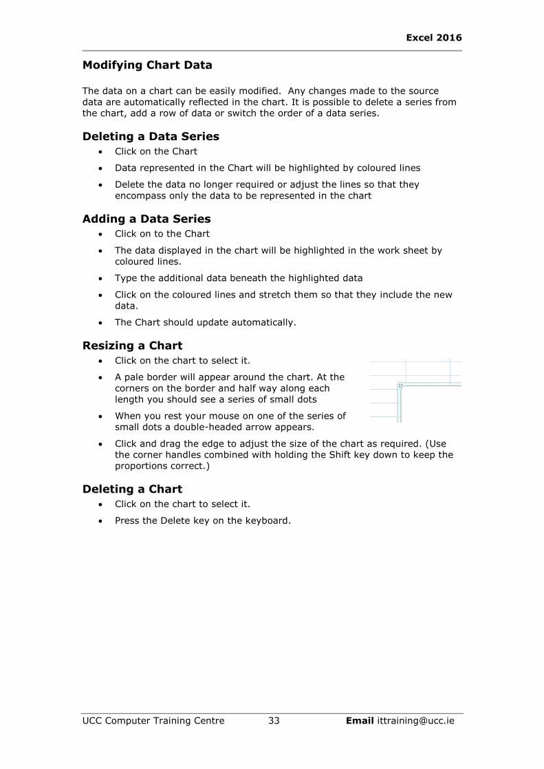
Resizing a Chart

• Click on the chart to select it.

• A pale border will appear around the chart. At the

corners on the border and half way along each

length you should see a series of small dots

• When you rest your mouse on one of the series of

small dots a double-headed arrow appears.

• Click and drag the edge to adjust the size of the chart as required. (Use

the corner handles combined with holding the Shift key down to keep the

proportions correct.)

Deleting a Chart

• Click on the chart to select it.

• Press the Delete key on the keyboard.

Excel 2016


Pivot Tables

A PivotTable is an interactive table that contains

summarised data. Once a pivot table has been created, you

can manipulate it to analyse your data in different ways.

There are times when you may want to quickly summarise

your worksheet information in different ways for different

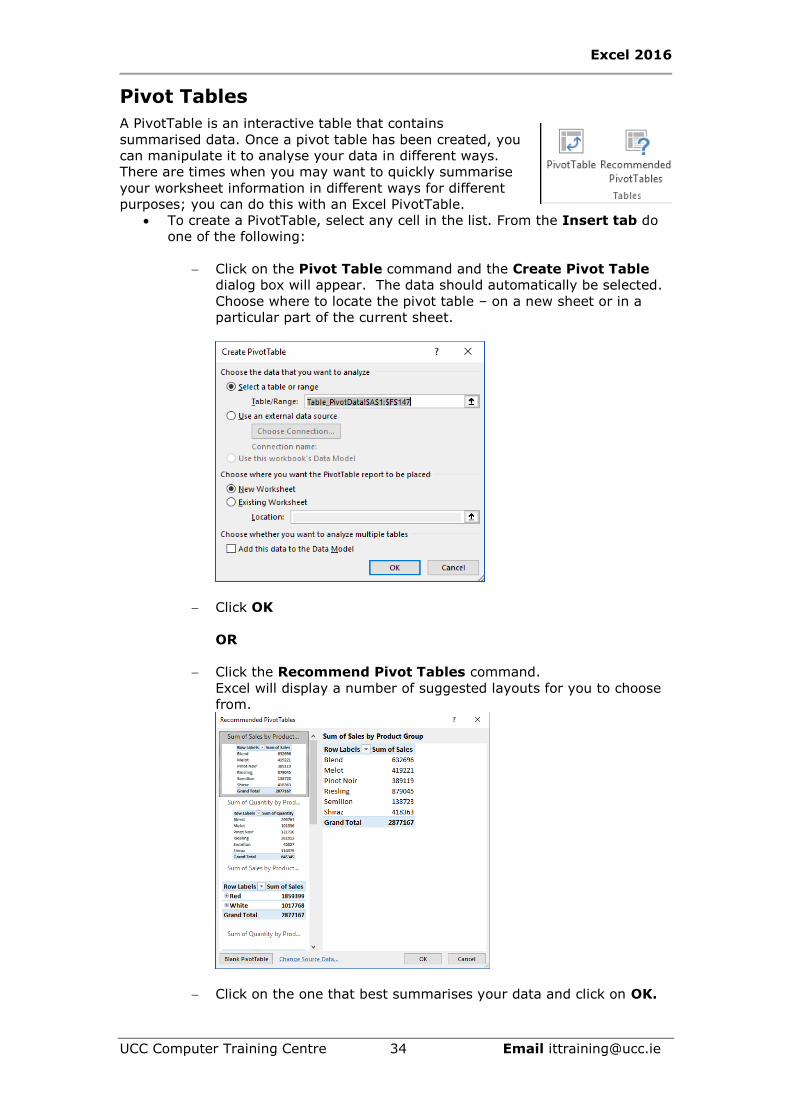
purposes; you can do this with an Excel PivotTable. • To create a PivotTable, select any cell in the list. From the Insert tab do

one of the following:

− Click on the Pivot Table command and the Create Pivot Table

dialog box will appear. The data should automatically be selected.

Choose where to locate the pivot table – on a new sheet or in a

particular part of the current sheet.

− Click OK

OR

− Click the Recommend Pivot Tables command.

Excel will display a number of suggested layouts for you to choose

from.

− Click on the one that best summarises your data and click on OK.

Excel 2016


• Once the Pivot Table is created all pivot table options are available within

the Pivot Table Tools under both the Analzye and Design tabs.

• This is displayed once you click anywhere on the Pivot Table.

▪ Arrange the layout of your pivot table by dragging the headings from the

field list on the right hand side to the Report filter, column labels, row

labels and values areas beneath

• Once you have picked where to have the different headings your pivot

table will appear.

Excel 2016


• You don’t have to use all the fields and a little experimentation is required

initially to decide what layout works best.

− The heading in the values field nearly always represents a numeric

value. A value you would want to sum, average or count.

− The heading in the Report Filter is something you might want to

filter an entire set of data on. In this example, it might be useful to

compare the different stores.

▪ Using the drop-down arrows on the headings you can filter the data.

Changing the Value Field Settings

By default, if you have a numeric value in the Values field it will be summed. If

you want to get the average of count the number of values, do the following

▪ Click on the Arrow beside the Field Heading

in the VALUES on the Layout Pane on the

right of the screen or right click somewhere

within the Values area of the Pivot Table

▪ From the menu that displays select Value

Field Settings

▪ Choose your preferred option for example

Average, or Max

▪ The number format can also be changed

here e.g. if you required Currency with 2 decimal places

▪ Click OK

Refreshing the Data

If changes are made to the original data you must Refresh your pivot table to

reflected these changes. The Refresh command is located under the Analyse Tab

of Pivot Table Tools.

Excel 2016


Pivot Charts

A PivotChart provides a graphical representation of the data in a PivotTable

report, in this case is called the associated PivotTable report. Like a PivotTable, a

PivotChart is interactive. When you create a PivotChart, PivotChart filters are

displayed in the chart area so that you can sort and filter the underlying data of

the PivotChart report. Changes that you make to the field layout and data in the

associated PivotTable are immediately reflected in the PivotChart.

A PivotChart displays data series, categories, data markers, and axes just as

standard charts do. You can also change the chart type and other options such as

the titles, the legend placement, the data labels, and the chart location.

Excel 2016


Quick Analysis Tool

The quick analysis tool is new since Excel 2013. This tool enables the user to

quickly access features like Conditional Formatting, Charts, Functions, Tables,

Pivot Tables, and Sparklines at the click of a button.

• Select the data you wish to analyse. The

Quick Analysis Tool button appears to the

bottom right of the data selection.

• The Quick Analysis Tool appears. This tool

has 5 different Tabs running along the top

and as you rest your mouse over the various buttons a preview of the

option appears on your on screen data.

1. FORMATTING – here you can access a number of conditional

formatting options

2. CHARTS – this allows to quickly insert a chart

3. TOTALS – here there is a number of built in functions and running

totals options. Note the arrow to the right of this box, click on it to the

display the second lot of options.

Excel 2016


4. TABLES – this tables allows you to quickly format your data as a Table

or to insert a Pivot Table

5. SPARKLINES - here you can access a number of sparkline options.

Excel 2016


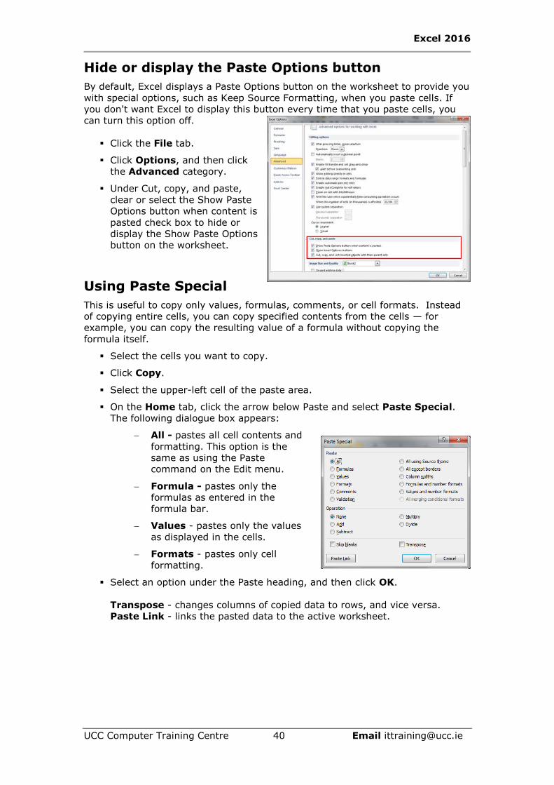
Hide or display the Paste Options button

By default, Excel displays a Paste Options button on the worksheet to provide you

with special options, such as Keep Source Formatting, when you paste cells. If

you don't want Excel to display this button every time that you paste cells, you

can turn this option off.

▪ Click the File tab.

▪ Click Options, and then click

the Advanced category.

▪ Under Cut, copy, and paste,

clear or select the Show Paste

Options button when content is

pasted check box to hide or

display the Show Paste Options

button on the worksheet.

Using Paste Special

This is useful to copy only values, formulas, comments, or cell formats. Instead

of copying entire cells, you can copy specified contents from the cells — for

example, you can copy the resulting value of a formula without copying the

formula itself.

▪ Select the cells you want to copy.

▪ Click Copy.

▪ Select the upper-left cell of the paste area.

▪ On the Home tab, click the arrow below Paste and select Paste Special.

The following dialogue box appears:

− All - pastes all cell contents and

formatting. This option is the

same as using the Paste

command on the Edit menu.

− Formula - pastes only the

formulas as entered in the

formula bar.

− Values - pastes only the values

as displayed in the cells.

− Formats - pastes only cell

formatting.

▪ Select an option under the Paste heading, and then click OK.

Transpose - changes columns of copied data to rows, and vice versa.

Paste Link - links the pasted data to the active worksheet.

Excel 2016


Object Linking and Embedding (OLE Linking)

Object Linking and Embedding allows you to share information between MS Office

programs such as Excel and Word. Linked and embedded objects look the same

but act differently.

Linked data is displayed in the destination file. It is stored in the source file and

updated only if you update the source file.

Embedded objects become part of the destination file and are not affected by any

changes in the source file. You can amend the embedded object by double-

clicking on it. It is automatically opened and edited using the source program if it

is available.

Embedding an Excel Worksheet in Word ▪ Select the Excel object or cells to embed.

▪ Click the Copy button in

Excel.

▪ Switch to Word and on

the Home tab, click on

the down arrow of the

Paste button and select

Paste Special

▪ From the Paste Special

box select Microsoft Excel

Worksheet Object.

▪ Click on OK

Note: If the Paste button is

used instead of Paste Special the data is displayed in Word in a Table format and

is not an embedded object.

To Edit an Embedded Worksheet in Word

▪ Double-click on the worksheet object.

▪ A worksheet window is displayed in the document, and the Excel toolbars

are displayed in place of the Word toolbars. Now you can edit the object.

▪ Click on the document, outside the worksheet window to return to Word.

Excel 2016


To Link an Excel Worksheet in Word ▪ Select the worksheet object or cells to embed.

▪ Click the Copy button in Excel.

▪ Switch to Word and on the

Home tab, click on the down

arrow of the Paste button and

select Paste Special

▪ Select the Paste link: option

button

▪ From the As box select Microsoft

Excel Worksheet Object

▪ Click on OK.

To Edit a Linked Worksheet in Word

▪ Double-click on the worksheet object

▪ The original file is opened in Excel and you can edit it.

▪ Save and close the worksheet.

▪ Any changes are stored in the source file and displayed in Word.

▪ Click on the document outside the worksheet object to return to Word.

Opening the Linked File

▪ When you re-open a Word document that is linked to an Excel worksheet

the following dialogue box is displayed:

▪ Click Yes to update changes or No if you do not wish for the document to

reflect the changes that were made in Excel.

Excel 2016


To break a Linked Worksheet in Word

To permanently remove the link between the word document and the original

source worksheet

• Open the word file containing the link

• Click on the File menu click on Info

• On the right of this screen click on Edit Links to Files

• The following screen is displayed:

• Ensure that the source file is selected and click on Break Link

Excel 2016


Protecting Your Work

There are several levels of protection that can be applied to a workbook. The

topmost level of protection is set on the file level. If users can’t access the file

itself, they won’t be able to change the information inside it. At the file level, you

have several different protection options:

▪ You can require users to enter a password just to open the file.

▪ You can require users to enter a password if they want to save changes to

the file.

▪ You can make the file read-only.

▪ You can have Excel create a backup copy of the file every time it is

modified.

Tip Do not forget your password or the file will be inaccessible.

Passwords are case sensitive. You must type the password exactly as it was

created, including uppercase and lowercase letters.

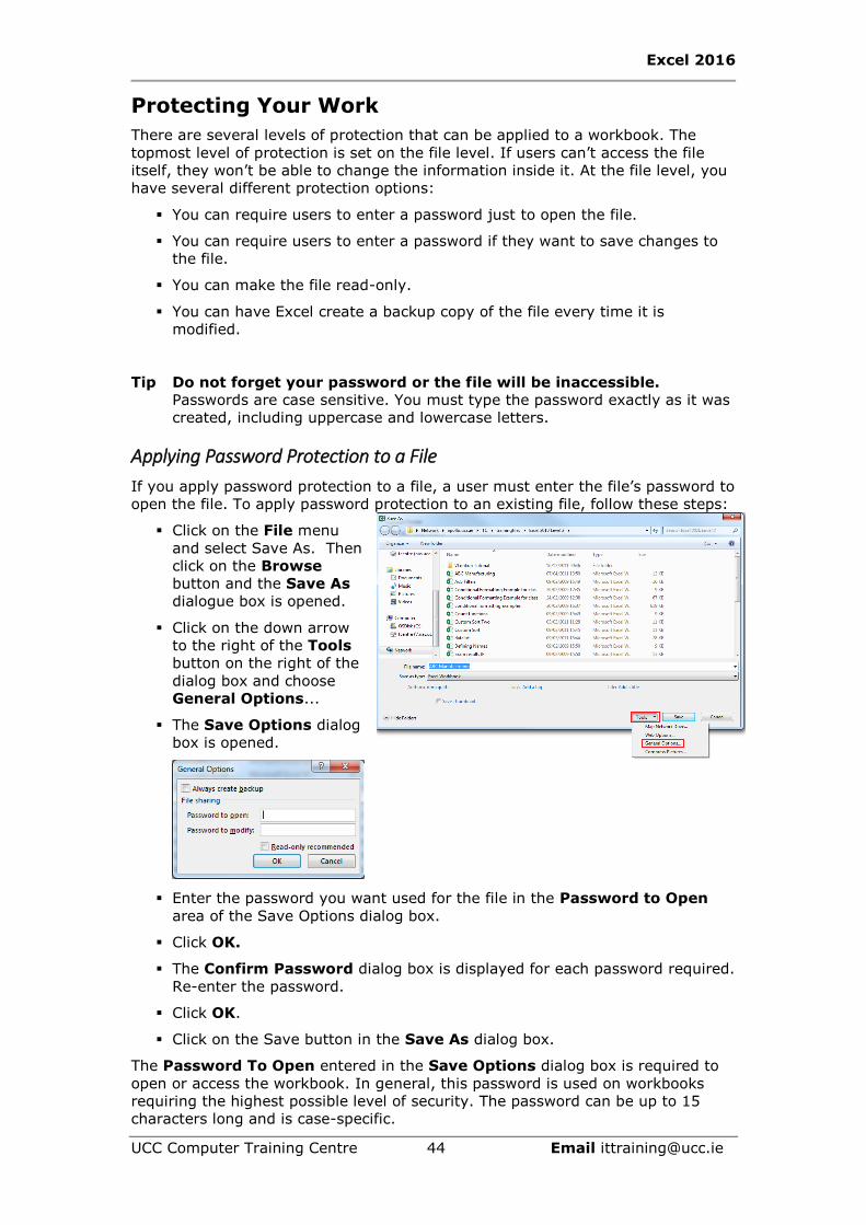
Applying Password Protection to a File

If you apply password protection to a file, a user must enter the file’s password to

open the file. To apply password protection to an existing file, follow these steps:

▪ Click on the File menu

and select Save As. Then

click on the Browse

button and the Save As

dialogue box is opened.

▪ Click on the down arrow

to the right of the Tools

button on the right of the

dialog box and choose

General Options...

▪ The Save Options dialog

box is opened.

▪ Enter the password you want used for the file in the Password to Open

area of the Save Options dialog box.

▪ Click OK.

▪ The Confirm Password dialog box is displayed for each password required.

Re-enter the password.

▪ Click OK.

▪ Click on the Save button in the Save As dialog box.

The Password To Open entered in the Save Options dialog box is required to

open or access the workbook. In general, this password is used on workbooks

requiring the highest possible level of security. The password can be up to 15

characters long and is case-specific.

Excel 2016


Applying a Modification Password

The Password To Open option requires the user to enter a password just to

open the file, but you can also set a password that the user must enter in order

to save modifications to the file. Entering a password in the Password To

Modify text box in the Save Options dialog box allows users to open the

workbook, but they cannot save changes to the workbook without knowing the

password.

Setting the Read-Only Recommended Option

The Read-Only Recommended setting is useful in two situations:

▪ When a workbook is used by more than one person, most of whom would

not be expected to make changes to it.

▪ When a workbook requires only periodic maintenance – users are

discouraged from accidentally changing a workbook that is not supposed to

be changed on a day-to-day basis.

When you set the Read-Only Recommended option in the Save Options dialog

box, Excel will display the following dialog box when the file is opened:

▪ Clicking on Yes opens the workbook as Read-Only, the text [Read-Only]

appears next to the file name on the title bar.

▪ Clicking on No, opens the file with full write privileges.

Protecting Data within the Workbook

The remainder of the security options serve to restrict what users can do after

they’ve opened the workbook.

There may be times when you’ll want to use worksheet protection to prevent

users from changing the contents of an individual sheet. For example, you want

users to be able to add data to this month’s sales sheet, but not to sheets for the

previous months.

Excel 2016


Protect an Individual Worksheet

▪ Switch to the worksheet you want to protect.

▪ Click on the Review Tab, and then click on

the Protect Sheet command.

▪ If required, enter a protection password for

the worksheet.

▪ Click on OK

Remove protection from an individual worksheet

▪ Switch to the worksheet you want to return to full access.

▪ Click on the Review Tab, and then click on the Unprotect Sheet command

and if prompted, enter the protection password for the worksheet.

Alternatively, the Protect Sheet option can be accessed from the Home Tab using

the Format command

Specify which cells can be changed after a worksheet is

protected

By default all cells are locked, therefore you must unlock the cells that you do

not want protected. This is done as follows:

▪ Select the cells you wish to be able to modify. To select non-adjacent cells

use the Ctrl key with the mouse.

▪ Right click on the selected cells and select

Format Cells. Click on the Protection

Tab.

▪ Clear the tick box to the left of Locked.

Note: this will have no effect until after

you protect the worksheet.

▪ Protect the worksheet by carrying out the

steps outlined previously. After you

protect the worksheet, the cells that you

unlocked in this procedure are the only

cells that can be changed.

Tip To move between unlocked cells on a protected worksheet, select an

unlocked cell, and then press TAB.

Excel 2016


Hiding Sheets and Cells Another method to discourage users from changing cells is by hiding all or part of

the sheet.

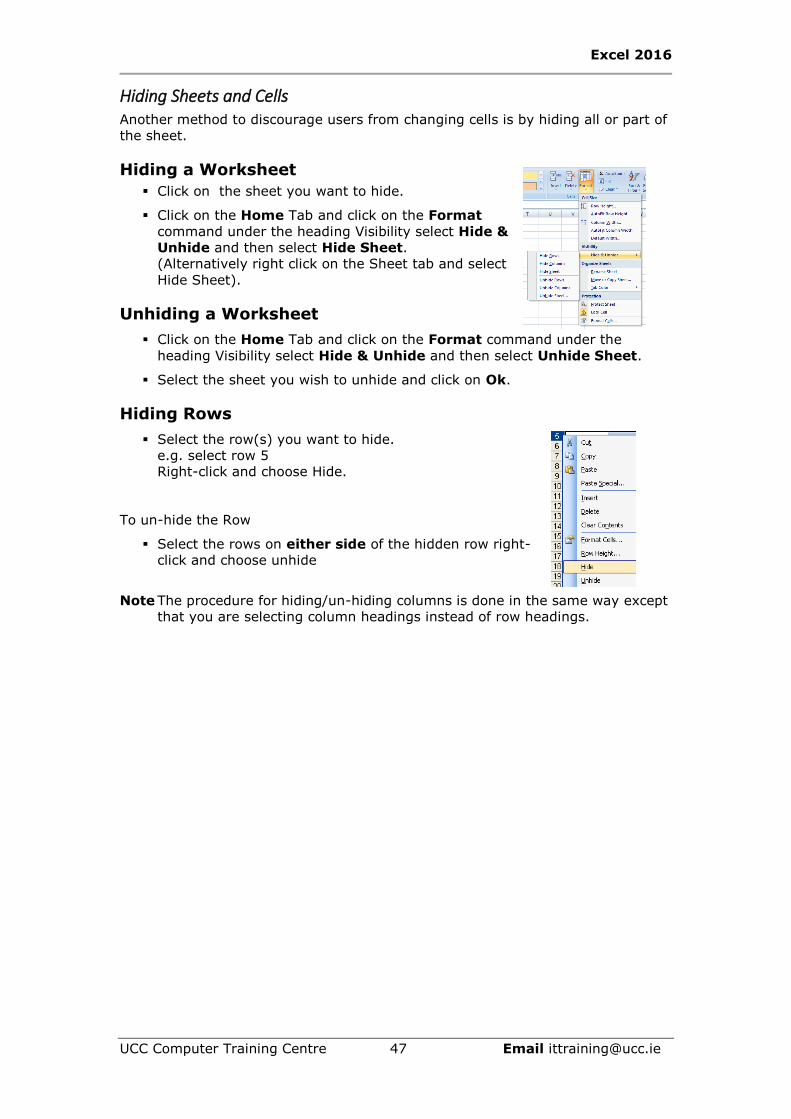
Hiding a Worksheet

▪ Click on the sheet you want to hide.

▪ Click on the Home Tab and click on the Format

command under the heading Visibility select Hide &

Unhide and then select Hide Sheet.

(Alternatively right click on the Sheet tab and select

Hide Sheet).

Unhiding a Worksheet

▪ Click on the Home Tab and click on the Format command under the

heading Visibility select Hide & Unhide and then select Unhide Sheet.

▪ Select the sheet you wish to unhide and click on Ok.

Hiding Rows

▪ Select the row(s) you want to hide.

e.g. select row 5

Right-click and choose Hide.

To un-hide the Row

▪ Select the rows on either side of the hidden row right-

click and choose unhide

Note The procedure for hiding/un-hiding columns is done in the same way except

that you are selecting column headings instead of row headings.

Excel 2016


Cell Comments

Comments can be attached to cells to document your work, explain calculations

and assumptions, or provide reminders.

Normally a red triangle appears in the upper right corner of a cell to indicate the

presence of a comment. When you move the mouse over a cell displaying this

indicator the comment is displayed. All comment options may be found under the

Review Tab

Add a comment to a cell

▪ Click the cell to which you want to add the comment.

▪ Right click and select Insert Comment.

( also available from the Review Tab).

▪ In the box, type the comment text.

▪ When you finish typing the text, click outside the

comment box.

Edit a comment

▪ Click the cell with the comment you want to edit.

▪ Right click and choose Edit Comment

Delete a comment

▪ Click the cell with the comment you want to delete.

▪ Right click and choose Delete Comment

Excel 2016


Print a worksheet with comments

If you want to print the comments in the positions where they appear on the

sheet, you must first display the comments that you want to print. To display all

comments, click Comments on the View menu. Move and resize the comments,

as necessary.

▪ To display an individual comment, right-click the cell that contains the

comment, and then click Show Comment on the shortcut menu.

▪ Click on the Page Layout Tab, click Page Setup dialogue box laucher, and

then click the Sheet tab.

The following dialogue box is displayed:

▪ To print the comments at the end of the

sheet, click on the down arrow to the right of

Comments and choose At end of sheet.

▪ To print the comments where they appear on

the worksheet, choose As displayed on

sheet.

Note: To print comments, you must also print the worksheet that contains them.

Excel 2016


Data Validation

Data validation is an Excel feature that you can use to define restrictions on what

data can or should be entered in a cell. You can configure data validation to

prevent users from entering data that is not valid. If you prefer, you can allow

users to enter invalid data but warn them when they try to type it in the cell. You

can also provide messages to define what input you expect for the cell, and

instructions to help users correct any errors.

▪ The data validation commands are located on

the Data tab, in the Data Tools group.

▪ You configure data validation in the Data

Validation dialog box.

▪ Click on the Settings Tab. Click on the

dropdown arrow to the right of Allow and

choose the required option.

▪ Example: if you want to restrict data to predefined items in a list, select List

and then type the values in the source box using a comma to separate

them. Alternatively, you may already have the values typed elsewhere in

the workbook and they can be selected with the

mouse.

• Input messages are generally used to offer users

guidance about the type of data that you want

entered in the cell.

• You can also choose to show an error alert

that appears only after users enter invalid

data.

• Then click on OK.

Excel 2016


Importing Data using the Text Import Wizard

Data created in different applications, can be imported into an Excel spreadsheet.

▪ Click on the File menu and select Open

or

if you already have Excel open, from the Data Tab under the group Get

External Data and click on From Text command.

▪ When selecting the file you wish to import, ensure that you have selected

All Files from the drop down list to the right of the File Name box or you

may not be able to see the required file.

▪ Click on Import or Open (depending on which method you used in the first

step above).

▪ The Text Import Wizard box is displayed:

▪ In Step 1 select either Delimited or Fixed width then click on Next >.

Some experimentation is required here as it may be difficult to separate all

the data neatly into columns.

▪ If you have selected Delimited in Step 1, in Step 2

select the appropriate delimiter character. This

character will vary depending on the contents of the

file you are importing. Tab is set by default.

▪ If you have selected Fixed width in Step 1, in Step 2

Excel attempts to divide the data into columns. Each

line with arrows is a column break. Set the field

widths (column breaks) using the following methods:

− to create a break line, click at the desired

position

− to delete a break line, double click on the line.

▪ to move a break line, click and drag it.

Click on Next >.

Excel 2016


▪ In Step 3 if necessary change the Column data format. In the example

below the last column has been selected and the data format has been

changed to Date: DMY.

▪ If there is a column of data that you do not wish to import, select the

column and then select Do not import column (skip).

▪ Click on Finish.

Tip Ensure that you save the file as an excel workbook when you are finished.

Excel 2016


Keyboard Shortcuts

Keyboard Shortcuts

Result in Excel 2016

F1 Key Help

F2 Key Edit current Cell

F4 Key To repeat the last action

F5 Key Goto

F7 Key Spell Check

F12 Key Save file as

CTRL and A Select entire worksheet.

CTRL and B Toggle Bold Text.

CTRL and C Copies the item or items selected to the

Clipboard

CTRL and F Displays the Find dialog box.

CTRL and H Displays the Replace dialog box.

CTRL and I Toggles Italic Text.

CTRL and N New File.

CTRL and O Open File.

CTRL and P Print.

CTRL and S Save File.

CTRL and U Toggles Underlined Text.

CTRL and V Paste the contents of the clipboard.

CTRL and X Cut the selected item.

CTRL and Y Redo the last undone action

CTRL and Z Undoes the last action.

CTRL and 1 Displays Format Cells Dialogue Box

CTRL and 5 Toggles Strikethrough Text

Formulas

ALT and = Autosum

ALT and F8 Macros

CTRL and ; Insert Current Date

CTRL and : Insert Current Time

Movement

Left Arrow One Cell Left (also SHIFT and TAB)

Right Arrow One Cell Right (also TAB)

Up Arrow / Down Arrow One Cell Up / One Cell Down

Home Go to Beginning of row

CTRL and Home Go to Top of Worksheet (A1)

CTRL and End Go to End of Worksheet

Cell Selection

CTRL and Spacebar Select the entire Column

SHIFT and Spacebar Select the entire Row

SHIFT and Arrow Keys ←↑↓→

Use for instead of the mouse for selecting cells

SHIFT and Right Cursor Select all cells to the right of the active one

Excel 2016


Notes

Microsoft Excel 2016 - ucc.ie · Excel 2016 UCC Computer Training Centre ii Email [email protected]...

Documents

Transcript of Microsoft Excel 2016 - ucc.ie · Excel 2016 UCC Computer Training Centre ii Email [email protected]...