Microsoft Excel 2010 - · PDF fileClick the Start button and choose All Programs > Microsoft...

Microsoft

Excel

2010

M i c r o s o f t E x c e l 2 0 1 0 - P a r t I

1

Part I: Introduction to MS Excel 2010

Microsoft Excel 2010 is a spreadsheet software in the new Microsoft 2010 Office Suite. Excel allows you to store, manipulate and analyze data in organized workbooks for home and business tasks. You can use Excel for to keep up with inventory, budgets, bookkeeping, contact lists, etc.

Getting Started

1. Click the Start button and choose All Programs > Microsoft Office > Microsoft Excel 2010. (Note: The Start button is disabled while in the training mode.)

2. Double click the Microsoft Excel icon on the desktop. 3. Whenever you start word, by default, a new blank document will appear in the

application window, and the Home tab is active by default.

Ribbon Tabs Title Bar

Quick Access Toolbar

Worksheet

Scroll Bar

Ribbon Groups


2

Components of the Excel Window

The tabbed Ribbon system was introduced in Excel 2007 to replace traditional menus. It contains all of the commands you'll need in order to do common tasks. There are multiple tabs, each with several groups of commands. Some groups have an arrow in the bottom-right corner that you can click to see even more commands

File Tab: Opens Backstage view, which displays a menu of commonly used file-management commands, such as Open, Save, Save As, and Print.

Quick Access Toolbar: Contains buttons for frequently used commands. By default, Save, Undo, and Repeat/Redo are available. You can customize the toolbar to include additional commands.

Ribbon Tabs: Contain Excel’s primary tools and commands, which are organized in logical groups and divided among the tabs. The main tabs are File, Home, Insert, Page Layout, References, Mailings, Review, and View.

Ribbon Groups: Further organize related tools and commands. For example, tools and menus for changing text formats are arranged together in the Font group.

Title Bar: Displays the name of the current document.

Document area: Displays the text graphics that you type, edit, or insert. The flashing vertical line in the document area is called the insertion point, and it indicates where text will appear as you type.

Status Bar: Contains the page number, word count, View commands, and document Zoom.

Scrollbars: Used to view parts of the document that doesn’t currently fit in the window. You can scroll vertically and horizontally.

Help: Pressing your F1 key will bring up the Help function for Window-based programs. Word 2010 offers relevant results with articles from different sources online.

The Ribbon

Understanding the Ribbon is a great way to help understand the changes between Microsoft 2003 to Microsoft 2010. The ribbon holds all of the information in previous versions of Microsoft Office in a more visual stream line manner through a series of tabs that include an immense variety of program features. The Ribbon contains multiple tabs, each with several groups of commands. You can add your own tabs that contain your favorite commands.

Home Tab-This is the most used tab; it incorporates all text and cell formatting features such as font and paragraph changes. The Home Tab also includes basic spreadsheet formatting elements such as text wrap, merging cells and cell style.

Insert Tab-This tab allows you to insert a variety of items into a document from pictures, clip art, and headers and footers.


3

Page Layout Tab-This tab has commands to adjust page such as margins, orientation and themes

Formulas Tab-This tab has commands to use when creating Formulas. This tab holds an immense function library which can assist when creating any formula or function in your spreadsheet.

Data Tab-This tab allows you to modifying worksheets with large amounts of data by sorting and filtering as well as analyzing and grouping data.

Review Tab-This tab allows you to correct spelling and grammar issues as well as set up security protections. It also provides the track changes and notes feature providing the ability to make notes and change someone’s document.

View Tab-This tab allows you to change the view of your document including freezing or splitting panes, viewing gridlines and hide cells.

Creating a New Workbook

1. Click File > New. Excel will display available templates. You can create a blank workbook or a blank template, or choose from a number of built-in templates. For a blank workbook click the Blank Workbook template, and click Create.

2. You can also press CTRL + N. New workbooks open in a separate window. When more than one workbook is open, you can switch between windows by clicking the View tab > Switch Windows, and selecting which window you want to view.


4

Opening an Existing Workbook

When you open a workbook, you’re viewing its contents in Excel but the original document will remain in the folder where it was saved.

Click the File tab > Open. Another option is to press Ctrl + O. The open file dialog box will appear, and you can choose which file you wish to open.

You can also view recently opened or viewed documents by choosing the Recent option under the File tab.

Pinned documents: Additionally, you can also “pin” any of the documents in the Recent Documents list so that they’ll always be displayed in this list. You can do so by clicking the pin icon to the right of the document name. Otherwise, as you open new documents, items on this list will move down and eventually moved off the list. To remove a recent document off the list, right-click and choose “Remove from list.” To remove all documents from the list, right-click any document and choose “clear unpinned items.”

Protected View: Word identifies documents from potentially unsafe locations and opens them in “protected view.” A document that was sent via email or from the Internet cannot be edited until you choose “Enable Editing” on the Message Bar (located at the top of the workbook). If you want to turn off this feature, go to Options under the File tab. In the Trust Center section of the dialog box, click Trust Center settings. Clear the desired options and click OK.

Saving a Workbook

Whenever you create a workbook, you will want to save your work. It is a good habit to save your work as often as you can while in the process of creating it. Unsaved work is often not recoverable, and all the work you will have put in will be lost. You can save your workbook by using the Save and Save As commands.

Using AutoRecover

When you’re working, you might forget to save regularly. If Excel closes unexpectedly, you may lose all your work since the last time you saved your document. Excel provides an automatic save feature that saves your document regularly. To customize or make sure this option is enabled:

1. On the File tab, click Options to open the Excel Options dialog box.

2. In the left pane, click Save to display the save options (as shown).


5

3. Check “Save AutoRecover information every…” 4. Enter your desired time of how often you want Excel to save your file. 5. Choose other options you desire. When you are done, click OK.

*Note: Choosing the “Keep the last Auto Recovered file if I close without saving” saves documents and drafts that you haven’t already saved. To recover a newly created file or unsaved document:

1. Click the File tab, and then Recent. 2. At the bottom of the window, click Recover Unsaved Documents. 3. Select the File and click Open. (You can save the document at this point.) 4. There may also be a Versions option, allowing you to choose which recovered

version you wish to open.

Printing a Workbook

Excel allows you to preview your workbook before printing. You can also specify settings such as orientation and page size. Click the File tab, then Print. If you are satisfied with your preview and do not wish to make changes, you can click on the Print button. Closing a Workbook

When you are finished working on a workbook and need to close it, Excel will prompt you to save it before it closes your workbook if you haven’t saved it that that point. On the File tab, click Close. You may also press Ctrl + W to close the workbook. To exit Excel, choose Exit or click on the Exit icon .

Working with Cells

Spreadsheets

The spreadsheet is represented by grids, with each cell bearing a specific reference:

Column – vertical reference (usually indicated by letters)

Row – horizontal reference (usually indicated by numbers)

Note: You may also notice that Excel spreadsheets are opened with three

worksheets by default (Sheet 1, Sheet 2,

Sheet 3). The amount of worksheets you

may have is dependent on your computer

memory. There is not set maximum

amount. You may also delete any unused sheets if desired.


6

The Cell

Each rectangle in a worksheet is called a

cell. A cell is the intersection of a row and a

column. Each cell has a name, or a cell

address, based on which column and row

it intersects. The cell address of a selected

cell appears in the Name box. Here you can

see that C5 is selected.

To Select a Cell:

1. Click on a cell to select it. When a

cell is selected you will notice that the

borders of the cell appear bold

and the column heading and row heading of the cell are highlighted.

2. Release your mouse. The cell will stay selected until you click on another cell in

the worksheet.

3. You can also navigate through your worksheet and select a cell by using the

arrow keys on your keyboard.

To Select Multiple Cells – Click and drag your mouse until all of the adjoining

cells you want are highlighted. Release your mouse. The cells will stay selected

until you click on another cell in the worksheet.

To select a single entire column – Click a column heading — that is, the letter

or letters that indicate the column.


7

To select multiple columns – Drag your mouse across multiple column

headings.

To select a single entire row – Click the row number.

To select multiple rows – Drag across multiple row numbers.

To select sequential cells – Click the first cell, hold down the Shift key, and

click the last cell you want.

To select non-sequential cells – Click the first cell, hold down the Ctrl key, and

click each additional cell (or row or column) you want to select.

To select the entire worksheet – Click the small box located to the left of

column A and above row 1. Optionally, you can select all cells in a worksheet by

pressing Ctrl+A.

Working with Cells

Cells are the basic building blocks of a worksheet. Cells can contain a variety of content such as text, formatting attributes, formulas, and functions (i.e., letters, numbers, dates, formulas, and functions.)

To Insert Content:

1. Click on a cell to select it.

2. Enter content into the selected

cell using your keyboard. The

content appears in the cell and in

the formula bar. You also can

enter or edit cell content from the

formula bar.

To Delete Content Within Cells:

1. Select the cells which contain

content you want to delete.

2. Click the Clear command on the

ribbon. A dialog box will appear.

3. Select Clear Contents.

4. You can also use your keyboard's

Backspace key to delete content

from a single cell or Delete key

to delete content from multiple

cells.


8

To Delete Cells:

1. Select the cells that you want to

delete.

2. Choose the Delete command from the

Cell Group ribbon.

Note: There is an important difference

between deleting the content of a cell and deleting the cell itself. If you delete

the cell, by default the cells underneath it will shift up and replace the deleted cell.

To Copy and Paste Cell Content:

1. Select the cells you wish to copy. 2. Click the Copy command. The border

of the selected cells will change appearance.

3. Select the cell or cells where you want to paste the content.

4. Click the Paste command. The copied content will be entered into the highlighted cells.

To Cut and Paste Cell Content:

1. Select the cells you wish to cut. 2. Click the Cut command. The border of the selected cells will change

appearance. 3. Select the cells where you want to paste the content. 4. Click the Paste command. The cut content will be removed from the original cells

and entered into the highlighted cells.


9

To Drag and Drop Cells:

1. Select the cells that you wish to move.

2. Position your mouse on one of the outside edges of the selected cells. The mouse changes from a white cross

to a black cross with 4

arrows . 3. Click and drag the cells to the

new location. 4. Release your mouse and the

cells will be dropped there.

To Use the Fill Handle to Fill Cells:

1. Select the cell or cells containing the content you want to use. You can fill cell content either vertically or horizontally.

2. Position your mouse over the fill handle so that the white cross becomes a black cross .

3. Click and drag the fill handle until all the cells you want to fill are highlighted. 4. Release the mouse and your cells will be filled.


10

Columns and Rows

To Modify Column Width:

1. Position your mouse over the column line in the column heading so that the

white cross becomes a

double arrow . 2. Click and drag the column to

the right to increase the column width or to the left to decrease the column width.

3. Release the mouse. The column width will be changed in your spreadsheet.

To Set Column Width with a Specific Measurement:

1. Select the columns you want to modify. 2. Click the Format command on the Home

tab. The format drop-down menu appears.

3. Select Column Width. 4. The Column Width dialog box appears.

Enter a specific measurement.

5. Click OK. The width of each selected column will be changed in your worksheet.

6. Select AutoFit Column Width from the format drop-down menu and Excel will automatically adjust each selected column so that all the text will fit.


11

To Modify the Row Height:

1. Position the cursor over the row line so that the white

cross becomes a double

arrow .

2. Click and drag the row downward to increase the row height or upward decrease the row height.

3. Release the mouse. The height of each selected row will be changed in your worksheet.

To Set Row Height with a Specific Measurement:

1. Select the rows you want to modify.

2. Click the Format command on the Home tab. The format drop-down menu appears.

3. Select Row Height.

4. The Row Height dialog box appears. Enter a specific measurement.

5. Click OK. The selected rows heights will be changed in your spreadsheet.

6. Select AutoFit Row Height from the format drop-down menu and Excel will automatically adjust each selected row so that all the text will fit.


12

To Insert Rows:

1. Select the row below where you want the new row to appear.

2. Click the Insert command on the Home tab.

3. The new row appears in your worksheet.

Note: When inserting new rows, columns, or cells, you will see the Insert Options

button by the inserted cells. This button allows you to choose how Excel formats them. By default, Excel formats inserted rows with the same formatting as the cells in the row above them. To access more options, hover your mouse over the Insert Options button and click on the drop-down arrow that appears.

To Insert Columns:

1. Select the column to the right of where you want the new column to appear. For example, if you want to insert a column between A and B, select column B.

2. Click the Insert command on the Home tab. 3. The new column appears in your worksheet.


13

Note: By default, Excel formats inserted columns with the same formatting as the column to the left of them. To access more options, hover your mouse over the Insert Options button and click on the drop-down arrow that appears.

When inserting rows and columns, make sure you select the row or column by clicking on its heading so that all the cells in that row or column are selected. If you select just a cell in the row or column then only a new cell will be inserted.

To Delete Rows:

1. Select the rows you want to delete.

2. Click the Delete command on the Home tab.

3. The rows are deleted from your worksheet.

4. The rows are deleted


14

To Delete Columns:

1. Select the columns you want to delete.

2. Click the Delete command on the Home tab.

3. The columns are deleted from your worksheet.

To Merge Cells Using the Merge & Center Command:

1. Select the cells you want to merge together.

2. Select the Merge & Center command on the Home tab.

3. The selected cells will be merged and the text will be centered.

If you change your mind, re-click the Merge & Center command to unmerge the cells.


15

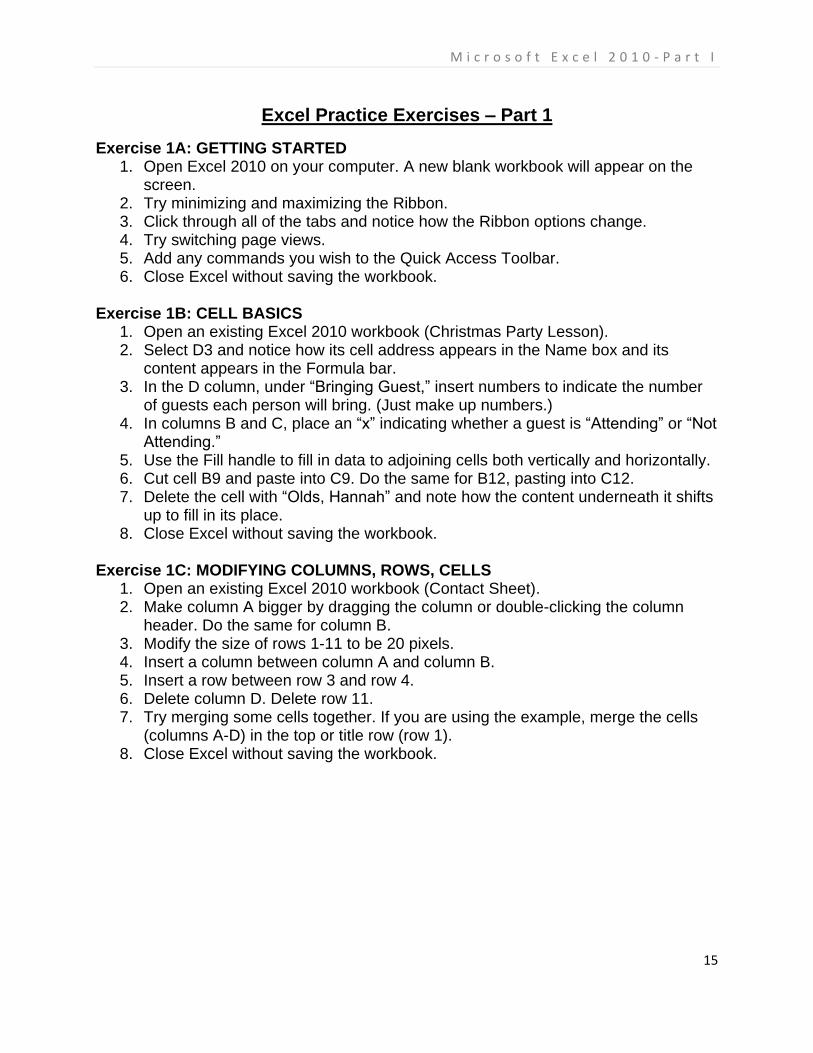
Excel Practice Exercises – Part 1

Exercise 1A: GETTING STARTED 1. Open Excel 2010 on your computer. A new blank workbook will appear on the

screen. 2. Try minimizing and maximizing the Ribbon. 3. Click through all of the tabs and notice how the Ribbon options change. 4. Try switching page views. 5. Add any commands you wish to the Quick Access Toolbar. 6. Close Excel without saving the workbook.

Exercise 1B: CELL BASICS

1. Open an existing Excel 2010 workbook (Christmas Party Lesson). 2. Select D3 and notice how its cell address appears in the Name box and its

content appears in the Formula bar. 3. In the D column, under “Bringing Guest,” insert numbers to indicate the number

of guests each person will bring. (Just make up numbers.) 4. In columns B and C, place an “x” indicating whether a guest is “Attending” or “Not

Attending.” 5. Use the Fill handle to fill in data to adjoining cells both vertically and horizontally. 6. Cut cell B9 and paste into C9. Do the same for B12, pasting into C12. 7. Delete the cell with “Olds, Hannah” and note how the content underneath it shifts

up to fill in its place. 8. Close Excel without saving the workbook.

Exercise 1C: MODIFYING COLUMNS, ROWS, CELLS

1. Open an existing Excel 2010 workbook (Contact Sheet). 2. Make column A bigger by dragging the column or double-clicking the column

header. Do the same for column B. 3. Modify the size of rows 1-11 to be 20 pixels. 4. Insert a column between column A and column B. 5. Insert a row between row 3 and row 4. 6. Delete column D. Delete row 11. 7. Try merging some cells together. If you are using the example, merge the cells

(columns A-D) in the top or title row (row 1). 8. Close Excel without saving the workbook.

M i c r o s o f t E x c e l 2 0 1 0 - P a r t I I

16

Part 2: Working with Rows, Columns, Formulas and Charts

Formulas

A formula is an equation that performs a calculation. Like a calculator, Excel can

execute formulas that add, subtract, multiply, and divide.

Creating Simple Formulas

Excel uses standard operators for equations:

plus sign for addition (+)

minus sign for subtraction (-)

asterisk for multiplication (*)

forward slash for division (/)

carat (^) for exponents.

The key thing to remember when writing formulas

for Excel is that ALL formulas must begin with an equal sign (=). This is because the

cell contains, or is equal to, the formula and its value.

To Create a Simple Formula in Excel: (Type in the data in the cells to follow the examples.)

1. Select the cell where the answer will appear (B4, for example).

2. Type the equal sign (=).

3. Type in the formula you want Excel to calculate. For example, "75/250".


17

4. Press Enter. The formula will be calculated and the value will be displayed in the

cell.

Creating Formulas with Cell References

When a formula contains a cell address, it is called a cell reference. (Type in the data in the cells to follow the examples.)



3. Type the cell address that

contains the first number in

the equation (B1, for

example).

4. Type the operator you need

for your formula. For example, type the addition sign (+).

5. Type the cell address that contains the second number in the equation (B2, for

example).


18


cell.

If you change a value in either B1 or B2, the total will automatically recalculate.

To Create a Formula using the Point and Click Method:



3. Click on the first cell to be included in the formula (A3, for example).


19

4. Type the operator you need for your formula. For example, type the

multiplication sign (*).

5. Click on the next cell in the formula (B3, for example).


cell.

To Edit a Formula:

1. Click on the cell you want to edit.

2. Insert the cursor in the formula bar and

edit the formula as desired. You can also

double-click the cell to view and edit

the formula directly from the cell.

3. When finished, press Enter or select the

Enter command .

4. The new value will be displayed in the

cell.

Note: If you change your mind, use the

Cancel command in the formula bar to

avoid accidentally making changes to your

formula.


20

Sorting Data

MS Excel also makes it easy for you to sort data whether it is alphabetical or by other criteria. You may choose to sort a section or the entire spreadsheet. You may access this command in two places: Home > Editing Group or Data > Sort & Filter Group.

To Sort in Alphabetical Order:

1. Select a cell in the column you want to sort by. In this example, we will sort by Last Name.

2. Select the Data tab, and locate the Sort and Filter group.

3. Click the ascending command to Sort

A to Z, or the descending command to Sort Z to A. 4. The data in the spreadsheet will be organized alphabetically.


21

To Sort in Numerical Order:

1. Select a cell in the column you want to sort by.

2. From the Data tab, click the ascending command to Sort Smallest to

Largest, or the descending command to Sort Largest to Smallest. 3. The data in the spreadsheet will be organized numerically.

To Sort by Date or Time:

1. Select a cell in the column you want to sort by.

2. From the Data tab, click the ascending command to Sort Oldest to Newest,

or the descending command to Sort Newest to Oldest. 3. The data in the spreadsheet will be organized by date or time.


22

To Sort in the Order of Your Choosing:

1. From the Data tab, click the Sort command to open the Sort dialog box.

2. Identify the column you want to Sort by by clicking the drop-down arrow in the Column field.

3. Make sure Values is selected in the Sort On field.

4. Click the drop-down arrow in the Order field, and choose Custom List...

5. Select NEW LIST, and enter how you want your data sorted in the List entries box.

6. Click Add to save the list, then click OK. 7. Click OK to close the Sort dialog box and sort your data.

Sorting Multiple Levels:

Another feature of custom sorting, sorting multiple levels allows you to identify which columns to sort by and when, giving you more control over the organization of your data.

To Add a Level:

1. From the Data tab, click the Sort command to open the Sort dialog box. 2. Identify the first item you want to Sort by 3. Click Add Level to add another item. 4. Identify the item you want to sort by next. 5. Click OK.

To Change the Sorting Priority:

1. From the Data tab, click the Sort command to open the Custom Sort dialog box.

2. Select the level you want to re-order.

3. Use the Move Up or Move Down arrows. The higher the level is on the list, the higher its priority.

4. Click OK.


23

Charts

Excel workbooks can contain a lot of data, and that data can often be difficult to

interpret. Excel has many different types of charts, so you can choose one that most

effectively represents the data.

To Create a Chart:

1. Select the cells that you want to chart, including the column titles and the row

labels. These cells will be the source data for the chart.

2. Click the Insert tab.

3. In the Charts group, select the desired chart category (Column, for example).

4. Select the desired chart type from the drop-down menu (Clustered Column, for

example).


24

5. The chart will appear in the worksheet.

Other Features

Page Setup

When you create a workbook, you need to tell Word how you want the page to be set up.

Size – On the Page Layout tab, click the Size button, and select the size of the paper you desire from the gallery. Note: If the size you want is not given as an option, click More Paper Sizes and specify your size.

Margins – Click the Margins button and select the margins you want. The standard is a 1-inch margin on all sides of the paper. Note: If the margin size you want is not given as an option, click Custom Margins and specify the margin size you want.

Orientation – When you click the Orientation button, you are asked whether you want your page oriented as a Portrait (longer than wide) or as Landscape (wider than long).

Find and Replace Functions

Microsoft Excel makes it easy for you to locate and replace

data in your spreadsheet. On the Home Tab, go to Editing to

select the Find and Replace tool (as shown to the right).

Type in the value you want to search and/or replace.

While the Find feature searches specified values throughout

the spreadsheet, the Replace feature allows you to find occurrences of a value and

replace it with another value.


25

Excel Practice Exercises – Part 2

Exercise 2A: CREATING SIMPLE FORMULAS 1. Open an existing Excel workbook (Summer Remodeling). 2. Write a simple division formula. If you are using the example, write the formula in

cell B18 to calculate the painting cost per square foot (total = square feet / total cost).

3. Write a simple addition formula. If you are using the example, write the formula in cell F5 to calculate the "Total Budget” (Sum of F3 and F4).

4. Write a simple subtraction formula. If you are using the example, subtract the "Expand Bathroom" cost (C6) from the "Total" cost (C11). Calculate your answer in C12.

5. Close Excel without saving. Exercise 2B: WORKING WITH BASIC FUNCTIONS

1. Open an existing Excel 2010 workbook (Office Supply). 2. Create a function that contains more than one argument. 3. Use AutoSum to insert a function. If you are using the example, insert the MAX

function in cell E15 to find the highest priced supply. 4. Insert a function from the Functions Library. If you are using the example, find the

PRODUCT function (multiply) to calculate the Unit Quantity times the Unit Price in cells F19 through F23.

5. Use the Insert Function command to search and explore functions. 6. Close Excel without saving.

Exercise 2C: WORKING WITH CHARTS

1. Open an existing Excel workbook (Book Sales). 2. Use worksheet data to create a chart. (Select the data you wish to include in the

chart.) 3. Change the chart layout (any layout you wish). 4. Apply a chart style (any layout you wish). 5. Move the chart to a different place in the worksheet. 6. Close Excel without saving.

Exercise 2D: SORTING DATA

1. Open an existing Excel workbook (T Shirt Order).

2. Sort column A in ascending by Homeroom #. 3. Add a second level, and sort it according to the last name (column C) in

ascending order (A-Z). 4. Change the sorting from the last name to the T-Shirt size (column F) from

smallest to largest. 5. Close Excel without saving.

Microsoft Excel 2010 - · PDF fileClick the Start button and choose All Programs > Microsoft...

Documents

Transcript of Microsoft Excel 2010 - · PDF fileClick the Start button and choose All Programs > Microsoft...