Microscopic Studies of Spin-Lattice Couplings · Master’s Thesis Department of Physics University...
71
Master’s Thesis Department of Physics University of Konstanz Microscopic Studies of Spin-Lattice Couplings Werner Schosser Matriculation Number: 01/738819 First Reviewer: Jun.-Prof. Dr. Fabian Pauly Second Reviewer: Prof. Dr. Ulrich Nowak November 2015
Transcript of Microscopic Studies of Spin-Lattice Couplings · Master’s Thesis Department of Physics University...

Master’s Thesis
Department of PhysicsUniversity of Konstanz
Microscopic Studiesof
Spin-Lattice Couplings
Werner Schosser
Matriculation Number: 01/738819
First Reviewer: Jun.-Prof. Dr. Fabian PaulySecond Reviewer: Prof. Dr. Ulrich Nowak
November 2015

2

Abstract
In the following Master’s thesis the spin-lattice couplings of the 3d transition metals iron andcobalt are examined. For the observation dimers of the metals are used.
To determine the exchange energy between the two single atoms in the system, they are splitup into two separate fragments. Then the interactions between the two subsystems for variousspin orientations of the subsystem’s spins and distances between the atoms are computed.
With the resulting spin dependent energy landscape, a semi-classical Hamilton operator thatincludes the spin-lattice couplings is built up.Subsequently the single terms of the Hamiltonian are discussed.
ZusammenfassungIn der vorliegenden Masterarbeit wird die Spin-Bahn-Kopplung der 3d Ubergangsmetalle Eisenund Kobalt anhand von Dimeren dieser Stoffe untersucht.
Dazu wird der spinabhangige Teil der Austauschenergie zwischen den beiden Einzelatomencharakterisiert. Um dies zu bewerkstelligen, wird das Dimer in zwei separate Fragmente ges-palten. Anschließend wird fur verschiedene Spinorientierungen der Teilsysteme und fur unter-schiedliche Atomabstande die Wechselwirkungsenergie berechnet.
Anhand der resultiernden spinabhangigen Energielandschaften wird ein semiklassischer Hamilton-operator hergeleitet, der das System bescheibt und die verschiedenen Spin-Bahn-Kopplungstermeenthalt. Anschließend werden die enthaltenen Kopplungsterme diskutiert.
3

4
Contents
1 Introduction 7
2 Density Functional Theory 92.1 Schrodinger Equation . . . . . . . . . . . . . . . . . . . . . . . . . . . . . . . . 92.2 Variational Principle for the Ground State . . . . . . . . . . . . . . . . . . . . . 102.3 Electron Density . . . . . . . . . . . . . . . . . . . . . . . . . . . . . . . . . . 112.4 Hohenberg-Kohn Theorems . . . . . . . . . . . . . . . . . . . . . . . . . . . . . 112.5 The Kohn-Sham Approach . . . . . . . . . . . . . . . . . . . . . . . . . . . . . 122.6 The LCAO Ansatz in the Kohn-Sham Approach . . . . . . . . . . . . . . . . . . 142.7 Dirac Equation . . . . . . . . . . . . . . . . . . . . . . . . . . . . . . . . . . . 142.8 Relativistic DFT . . . . . . . . . . . . . . . . . . . . . . . . . . . . . . . . . . . 16
3 Rotation Algebra in Relativistic Quantum Mechanics 213.1 Spin Rotation . . . . . . . . . . . . . . . . . . . . . . . . . . . . . . . . . . . . 213.2 Spatial Rotation . . . . . . . . . . . . . . . . . . . . . . . . . . . . . . . . . . . 223.3 Rotation Transformations of Operators . . . . . . . . . . . . . . . . . . . . . . . 243.4 Transformation of the Dirac Equation . . . . . . . . . . . . . . . . . . . . . . . 263.5 Transformation of Orbitals . . . . . . . . . . . . . . . . . . . . . . . . . . . . . 27
4 The Systems 31
5 Results 355.1 Iron . . . . . . . . . . . . . . . . . . . . . . . . . . . . . . . . . . . . . . . . . 365.2 Cobalt . . . . . . . . . . . . . . . . . . . . . . . . . . . . . . . . . . . . . . . . 47
6 Outlook 55
7 Conclusion 59
A Additional calculations 65
B Erklarung 71
5

CONTENTS
6
Chapter 1
Introduction
Spin interactions and spin-lattice couplings are of central meaning in modern quantum physics.A problem that is still poorly understood since its discovery in 1915, is the transfer and con-servation of the angular momentum in the Einstein-de Haas [EdH1915] or the Barnett effect[Barn1915], which are actually based on spin-lattice couplings. At that time these effects wereof revolutionary importance, as they were the only possibility to determine the gyromagneticratio of solids.
First attempts to describe this problem were made by Van Vleck [Vle40], who did not yet con-sider the conservation of the angular momentum. With the later treatment of this subject by manyscientists, this was corrected. Lots of researchers launched out into formulating various theoriesabout this problem, e.g. [Fed76], [Doh75] or [Fed77], just to mention a few. Most of these the-ories were based on a phenomenological foundation, by using parameters, that were determinedin extensive experiments.
Due to the appearance of micro- and nanomechanical devices in the last few years this topic be-came uptodate again. The Einstein-de Haas effect was observed in nanoscale systems [Wall06],and was tried to be explained by the movement of magnetic domain walls [Jaaf09]. Furthermore,new concepts were developed, like for example the concept of the phonon spin [Zan14], whichwas adapted and expanded by [Gar15] to explain the angular momentum spin-phonon processes.
Another hot topic, related to spin-lattice couplings and magnetic anisotropies, are single moleculemagnets. These kind of magnetic particles show promise to be useful for data storage [Frie96],spintronics and quantum computing [Leh07], [Mas15]. Lots of new different molecular magnetsappeared with a large variety of topologies, containing transition metal atoms, like iron, cobalt,manganese or nickel [Hon09]. In these single molecule magnets magnetic anisotropy plays a bigrole, which is related to spin-lattice couplings.
Thus, it is important to be able to describe the spin and spin-orbit interactions in such systems.This Master’s thesis focuses on the spin interactions and spin-lattice couplings of one central partof those molecular magnets - the 3d transition metals iron, nickel and cobalt. Therefore, there are
7
CHAPTER 1. INTRODUCTION
especially dimers of these metals going to be studied by mapping the energy landscape dependenton the directions of the atomic spins and the distance of the atomic nuclei. Ab-initio calculationsare performed, by doing relativistic density functional theory using the code Turbomole. Fromthese mappings a Hamiltonian will be built up to describe these systems in a semi classical way,including the relevant spin-lattice couplings.
The thesis is structured as the follows. In chapter 2 and 3 the theoretical background is pre-sented. Chapter 2 describes the basics of on the one hand non-relativistic and on the other handrelativistic density functional theory. Chapter 3 presents the rotation algebra, that is used to im-plement a rotation tool into the Turbomole code, whereas chapter 4 describes the procedure ofthe made simulations, the results of which are presented and discussed in chapter 5. Finally anoutlook on further calculations is given.
8
Chapter 2
Density Functional Theory
In this chapter an introduction to density functional theory (DFT) will be given.First, the Schrodinger equation in the Born-Oppenheimer approximation will be introduced anda method for determining the ground state of a system will be given. Moreover, the Hohenberg-Kohn equations and the LCAO approach will be presented. Finally, it will be shown how thistheory can be expanded into a two-component DFT, which includes relativistic effects, like spin-orbit interactions.The first part of this chapter is mainly based on [Ko01], [Bar01] and [Per96], whereas the second,relativistic part is based on [Arm08], [Eng02] and [Arm06].
2.1 Schrodinger EquationUsually, one describes a molecular system with M atomic nuclei and N electrons (M, N ∈N) bysolving the time independent Schrodinger equation
H ψi
(~x1, . . . ,~xN ,~R1, . . . ,~RM
)= Eiψi
(~x1, . . . ,~xN ,~R1, . . . ,~RM
)(2.1)
with the coordinates of the nuclei ~RK and the coordinates of the electrons~xi = (~ri,si), includingthe spatial coordinates~ri and the spin coordinates si for K = 1, . . . ,M and i = 1, . . . ,N.The used Hamilton operator is given by
H =−12
N
∑i=1
~∇2i︸ ︷︷ ︸
(I)
−12
M
∑K=1
1MK
~∇2K︸ ︷︷ ︸
(II)
−N
∑i=1
M
∑K=1
ZK
riK︸ ︷︷ ︸(III)
+N
∑i=1
N
∑j=i+1
1ri j︸ ︷︷ ︸
(IV )
+M
∑K=1
M
∑L=K+1
ZKZL
RKL︸ ︷︷ ︸(V )
, (2.2)
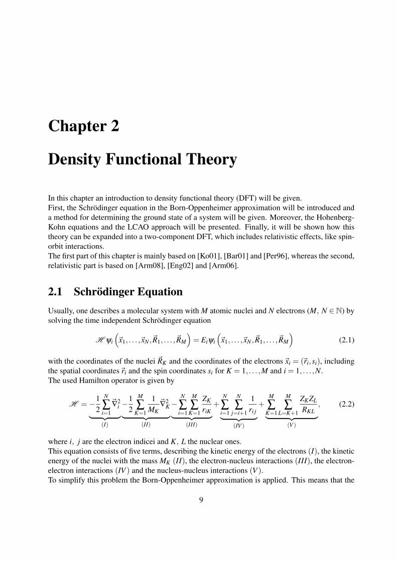
where i, j are the electron indicei and K, L the nuclear ones.This equation consists of five terms, describing the kinetic energy of the electrons (I), the kineticenergy of the nuclei with the mass MK (II), the electron-nucleus interactions (III), the electron-electron interactions (IV ) and the nucleus-nucleus interactions (V ).To simplify this problem the Born-Oppenheimer approximation is applied. This means that the
9
CHAPTER 2. DENSITY FUNCTIONAL THEORY
position of the nuclei is considered as being constant and thus the electrons move in a fixed field.This assertion is valid, as the electrons are much faster than the nuclei on account of their - incomparison to a nucleus - negligibly small mass.This approximation leads to the following electronic Hamiltonian
He =−12
N
∑i=1
~∇2i −
N
∑i=1
M
∑K=1
ZK
riK+
N
∑i=1
N
∑j=i+1
1ri j
=: T +VNe +Vee, (2.3)
where VNe is called the external potential. In general, this term can include electric or magneticfields in addition to the field from the nuclei.Comparing Eq. (2.3) to Eq. (2.2) it can be noticed that, since the position of the nuclei is constant,their kinetic energy (Eq. (2.2)(II)) vanishes. For the same reason, the nucleus-nucleus interac-tions (Eq. (2.2)(V)) become constant and it is not necessary to consider these terms in furthercalculations.
2.2 Variational Principle for the Ground StateAs mentioned before, the Schrodinger equation Eq. (2.1) has to be solved.Using the approximation, discussed in the previous section, the problem is described by thereduced electronic Schrodinger equation
Heψe = Eeψe. (2.4)
In the following we abandon to flag this with the subscript e.The big issue to solve this Schrodinger equation is the large amount of 4N degrees of freedom,which prevent the equation to be solved exactly. Nonetheless, there is a method to approximatethe many electron wave function of the systems ground state. This method is called the varia-tional principle. It is based on the fact, that any normalized test wave function ψtest will have agreater or equal energy expectation value than the wave function ψ0 of the ground state expressedby
〈ψtest|H |ψtest〉= Etest ≥ E0 = 〈ψ0|H |ψ0〉 . (2.5)
The equality Etest = E0 only holds only for ψtest = ψ0.In order to find the ground state, the functional E [ψtest] can be minimized in consideration of allof the allowed N electron wave functions
E0 = minψ(N)
E[ψ
(N)]= min
ψ(N)
⟨ψ
(N)∣∣∣T +VNe +Vee
∣∣∣ψ(N)⟩. (2.6)
This also means that the energy of the ground state E [N,VNe] is a functional of the externalpotential VNe and the electron number N.
10

CHAPTER 2. DENSITY FUNCTIONAL THEORY
2.3 Electron DensityThe electron density ρ (~r) is an observable, that embodies the probability of finding an electronin the infinitesimal volume d~r. So it can be defined as
ρ (~r) = N∫|ψ (~x1, . . . ,~xN) |2ds1d~x2 . . .d~xN , (2.7)
the integral of the absolute value of the wave function over all electron coordinates except thespatial part of an arbitrary one multiplied by N. This definition can only be made because theelectrons are indistinguishable. Here~r1 is chosen w.l.o.g..Since the electron density is a probability, it has three special properties, namely it is positive, itvanishes at infinity and it is normalized,
ρ (~r) ≥ 0 (2.8)lim|r|→∞
ρ (~r) = 0 (2.9)
1N
∫V
ρ (~r)d~r = 1. (2.10)
Normalization is often used to double-check the consistency of the electron density in DFTcalculations.
2.4 Hohenberg-Kohn TheoremsTo describe a system it is efficient to use its electron density instead of the molecular wavefunction, since the degrees of freedom are severely reduced from 4N to 3, as it is used in modernDFT. These calculations are based on the two Hohenberg-Kohn theorems, that are presented inthe following. In order to focus on the aim of applying their statement to DFT it is abstainedfrom showing the proofs, which can be found for example in [Ho64].
1. The first Hohenberg-Kohn theorem states that a system with N electrons in an externalpotential VNe is completely described by its ground state electron density, that thereforedefines the Hamiltonian uniquely. It is
E [ρ0] = ENe [ρ0]+T [ρ0]+Eee [ρ0]︸ ︷︷ ︸=:FHK
=∫
ρ (~r)VNe (~r)d~r+FHK [ρ0] , (2.11)
with the Hohneberg-Kohn functional FHK [ρ]. This functional is universal for all systems,but its explicit form is not known. If it was, finding the exact solution of the Schrodingerequation would be possible.Nevertheless, the Coulomb interaction J [ρ] can be separated from the electron-electroninteraction term
Eee [ρ] =12
∫ ∫ρ (~r1)ρ (~r2)
r12d~r1d~r2 +Encl [ρ] = J [ρ]+Encl [ρ] , (2.12)
that converts the functional to a more convenient form.
11

CHAPTER 2. DENSITY FUNCTIONAL THEORY
2. The second Hohenberg-Kohn theorem is a version of the variational principle, that wasmentioned before, concerning the electron density. It states that the energy functionalE [ρ] yield the ground state energy if and only if the ground state electron density ρ0 isinserted. For all other densities ρ ′ 6= ρ0 it is
E0 < E[ρ′]= T
[ρ′]+ENe
[ρ′]+Eee
[ρ′] , (2.13)
and, therefore, E [ρ ′] is an upper bound for the true value of the ground state energy for allelectron densities.
It is important to mention that these theorems hold for the ground state only, but not for anyexcited states.
2.5 The Kohn-Sham ApproachIn order to find the ground state energy E0 we have to minimize the energy functional E [ρ] (seesecond Hohneberg-Kohn theorem)
E0 = minρ(N)
(∫ρ (~r)VNe (~r)d~r+FHK [ρ]
), (2.14)
concerning all allowed N electron densities ρ(N). As mentioned before, the Hohenberg-Kohnfunctional FHK [ρ] = T [ρ]+J [ρ]+Encl [ρ] has an unknown form, except the Coulomb part J [ρ].This means that an expression for it has to be found. Generally, this is very difficult.Walter Kohn and Lu J. Sham found a good way to approximate the problem. They treated thesystem as a perturbated non-interacting auxiliary system. The electron density ρS of this system
ρS =N
∑i=0
∑s|ψi (~r,s) |2 = ρ (~r) (2.15)
is the same as the one in the basis system. ψi are the orbitals of the auxiliary system. The kineticenergy of the non-interacting system becomes
TS =−12
N
∑i=1〈ψi|~∇2|ψi〉 (2.16)
and can be calculated exactly.But there are still unknown parts of the energy of the real system. On the one hand there is thedifference of the kinetic energy of the real system to TS and on the other hand the non-classicalenergy Encl . Therefore, with the help of the newly defined exchange correlation energy EXC
EXC := (T [ρ]−TS [ρ])+(Eee [ρ]− J [ρ]) (2.17)
that will contain all unknown parts of the energy of the system, it is comfortable to write theHohenberg-Kohn functional in the following form:
FHK [ρ] = TS [ρ]+ J [ρ]+EXC [ρ] . (2.18)
12

CHAPTER 2. DENSITY FUNCTIONAL THEORY
The non-interacting reference system can be described by the common Hamiltonian
HS =−12
N
∑i(~∇2
i +VS (~ri)), (2.19)
with a potential VS. The wave functions of the system can be calculated by determining theKohn-Sham orbitals ψi by solving
fKSψi =
(−1
2~∇2 +VS (~r)
)ψi = εiψi (2.20)
and building the Slater determinant of them. fKS is called the Kohn-Sham operator.The centerpiece of the approach is to find the connection between the reference system and thereal one. This is done by using the variational principle. The exact derivation that can be foundin [Cap02]. The result is that the ψi have to fulfill the equation(
−12~∇2 +
[∫ρ (~r2)
r12d~r2 +VXC (~r1)−
M
∑A
ZA
r1A
])ψi =
(−1
2~∇2 +Veff (~r1)
)ψi = εiψi, (2.21)
while being orthonormal as well.Comparing Eq. (2.20) to Eq. (2.21) the equivalence of the both potentials VS and Veff becomeobvious
VS (~r)≡Veff (~r) =∫
ρ (~r2)
r12d~r2 +VXC (~r1)−
M
∑A
ZA
r1,A. (2.22)
Here, the unknown exchange potential VXC is defined by the following functional derivation
VXC :=δEXC
δρ. (2.23)
If the Kohn-Sham equations are to be solved, it has to be done iteratively, since the effectivepotential VS depends on the electron density ρ itself.It has to be mentioned that the spin of the electrons has not been considered. Therefore, spindegeneracy has to be assumed by following the restricted Kohn-Sham formalism. Moreover, itis possible to separate the electron density
ρ (~r) = ρα (~r)+ρβ (~r) (2.24)
into the two parts of the different spins α and β and calculate the densities by performing theunrestricted formalism (cf. [Jac12]). This has to be done if e.g. the exchange potential VXC isspin dependent.
13
CHAPTER 2. DENSITY FUNCTIONAL THEORY
2.6 The LCAO Ansatz in the Kohn-Sham ApproachTo solve the Kohn-Sham equations Eq. (2.21) numerically with a computer the equations haveto be brought in a suitable form. Therefore, one expresses the Kohn-Sham orbitals ψi by a linearcombination
ψi =L
∑µ=1
cµiηµ (2.25)
of a basis set of atomic orbitals B = η1, . . . ,ηL. By inserting the linear combination of atomicorbitals (LCAO) into the Kohn-Sham equation Eq. (2.20) results in
fKS (~r)L
∑µ
cµiηµ (~r) = εi
L
∑µ
cµiηµ (~r) , (2.26)
which leads to
L
∑µ
cµi
∫ην (~r) fKS (~r)ηµ (~r)d~r = εi
L
∑µ
cµi
∫ην (~r)ηµ (~r)d~r (2.27)
by multiplying both sides of the equation with an orbital basis function ην from the left side.Introducing the Kohn-Sham matrix FKS, defined by
FKSνµ =
∫ην (~r) fKS (~r)ηµ (~r)d~r (2.28)
and the orbital overlap matrix S with
Sνµ =∫
ην (~r)ηµ (~r)d~r, (2.29)
the eigenvalue problem is eventually found
FKSC = SCε, (2.30)
which is an equivalent expression of the Kohn-Sham equations. FKS and S are L×L matrices aswell as the coefficient matrix C, which consists of all coefficients cµi.
2.7 Dirac EquationIn the previous sections, only a non-relativistic quantum system has been discussed. What fol-lows is the description of a relativistic one.A relativistic quantum system is usually described by the Dirac equation
HDΨ(~r) = εΨ(~r) , (2.31)
14

CHAPTER 2. DENSITY FUNCTIONAL THEORY
with the relativistic Dirac operator
HD = c~α~p+(β −1)mc2 +V (~r), (2.32)
containing
αi =
(σi 00 σi
), i = x,y,z, β =
(I 00 I
), (2.33)
the momentum operator ~p and the mass m of the relativistic particle.The corresponding wave function Ψ(~r) is a four component spinor
Ψ(~r) :=(
ψ(~r)χ(~r)
):=
ψ1(~r)ψ2(~r)χ1(~r)χ2(~r)
. (2.34)
Since such four component calculations are very expensive, the problem has to be simplified.Thus, quantum chemistry usually separates the interesting electronic ψ from the positronic partχ of the spinor, because this reduces the problem to a two-component theory for relativistic elec-trons. There are many different transformation methods, like the Douglas-Kroll-transformation[Wol02]. Many of these transformations can be found in [Schwe02].As an example the Pauli-Hamilton operator is derived. Therefore, the Dirac equation will bewritten as a system of two coupled equations
V (~r)ψ(~r)+ c~σ~pχ(~r) = Eψ(~r) (2.35)~σ~pψ(~r)+
[V (~r)−2mc2]
χ(~r) = Eχ(~r), (2.36)
with the vector of the Pauli matrices ~σ = (σx, σy, σz)T .
It is possible to separate the positronic part χ(~r) from the second equation
χ(~r) =
(1
1+ E−V (~r)2mc2
)~σ~p2mc
ψ(~r). (2.37)
Inserting this relation in Eq. (2.36), the electronic part results in[1
2m~σ~p
(1
1+ E−V (~r)2mc2
)~σ~p+V (~r)
]ψ(~r) = Eψ(~r). (2.38)
The only problem this form has, is the fact that the potential operator V (~r) is in the denominator.That is why the corresponding term has to be expanded in a power series(
1
1+ E−V (~r)2mc2
)=
∞
∑n=0
(−1)n(
E−V (~r)2mc2
)n
. (2.39)
15
CHAPTER 2. DENSITY FUNCTIONAL THEORY
In the following, only first order terms are considered and terms of higher order are neglected.This results in p2
2m+V (~r)− p4
8m3c2︸ ︷︷ ︸Hmv
+h2
8m2c2~∇2V (~r)︸ ︷︷ ︸
HDarwin
+h
4m2c2~σ[(~∇V (~r)
)×~p]
︸ ︷︷ ︸HSO
ψ(~r) = Eψ(~r) (2.40)
with the Pauli-Hamilton operator. It can be seen that this operator has relativistic correctionsin addition to the non-relativistic terms, like the correction of the relativistic energy Hmv, theso-called Darwin term HDarwin, that describes corrections on the electrostatic potential. Fur-thermore the spin-orbit term HSO is included. It can be easily identified with a spin-orbit term,assuming a hydrogen kind of potential V (~r) =−Z/r, where Z is the atomic number. The part ofthe Hamiltonian becomes
HSO =h
4m2c2~σ[(~∇V (~r)
)×~p]=
Z2m2c2r3
~S ·~L, (2.41)
where~L is the angular momentum operator.
2.8 Relativistic DFTThe used DFT code Turbomole uses a two-component formalism to include relativistic effects,like spin orbit interaction, in electrical structures of atoms. This formalism is based on the spindependent Hamilton operator in the Born-Oppenheimer approximation
H = ∑i
[σ0h0 (i)+~σ ·~hSO (i)
]+Vee +VNN, (2.42)
including an effective one particle spin-orbit operator ~σ ·~hSO (i) as well as a spin independent oneparticle Hamiltonian h0 (i) that includes the kinetic energy of the electrons and their potentialenergy in the field of the nuclei. VNN is the repulsion of the nuclei. The single particle wavefunctions
ψk(~x) =(
ψαk (~r)
ψβ
k (~r)
)(2.43)
in the system become two-component spinors ψk(~r) with complex components ψα/β
k (~r). Thevector ~x = (~r,s) consists of the spatial coordinate ~r and the spin s, as it did in the previouschapters. With these single particle wave functions, it is possible to determine the Fock-Diracdensity matrix
γ(~x,~x′) = ∑k
ψk(~r)ψk (~r′) =
(γαα(~r,~r′) γαβ (~r,~r′)γβα(~r,~r′) γββ (~r,~r′)
), (2.44)
16
CHAPTER 2. DENSITY FUNCTIONAL THEORY
which includes on the one hand the particle number density n(~r,~r′) and on the other hand the spinvector density ~m(~r,~r′). Here the Kohn-Sham approximation is anticipated, whereby the problemis transformed to an effective single particle problem with N non interacting electrons. Thus, thewave function is given by the Slater determinant of the single particle wave functions. This topicwill be elaborated later in this section.The particle number density can be determined by building the spin trace of the Fock-Diracdensity matrix
n(~r,~r′) = tr[γ(~r,~r′)
]. (2.45)
Similar to the non-relativistic case, the particle number N is obtained by integrating∫n(~r,~r)d~r = N. (2.46)
The spin vector density can be determined by building the trace
~m(~r,~r′) = tr[~σγ(~r,~r′)
](2.47)
over the spin. This density provides the expectation value of the system’s whole spin⟨~S⟩=
12
∫~m(~r,~r)d3r. (2.48)
It has to be mentioned that due to the spin orbit interaction the spin ~S is not conserved anymore,since it does not commute with the Hamilton operator H in Eq. (2.42).The Fock-Dirac density matrix can be rewritten in terms of the particle number density and thespin vector density to achieve the more comfortable form
γ(~x,~x′) =12[σ0n(~r,~r′)+~σ ·~m(~r,~r′)
]. (2.49)
Similar to the non-relativistic case, the Kohn-Sham approach is used to simplify the calculations.In the following part the two-component Kohn-Sham equations are determined. Therefore, anall electron ansatz is assumed, so the spin independent part of the Hamilton operator
h0 (i) =−12~∇2
i +N
∑K
ZK
riK(2.50)
is a sum of the kinetic energy and the potential energy of the electrons in the nuclear field.Due to the fact, that the spin-orbit coupling and the kinetic energy are non-local operators wecannot study them separately, so we have to calculate the exact energy including the spin-orbitinteraction
T = 〈Ψ|∑i−1
2~∇2
i +~σ ·~hSO (i)|Ψ〉 (2.51)
= TS [n(~r) ,~m(~r)] (2.52)
17

CHAPTER 2. DENSITY FUNCTIONAL THEORY
as one term, which is a functional of the particle density n(~r) and the spin vector density ~m(~r) =∫~σψ (~x1, . . . ,~xN)ψ∗ (~x1, . . . ,~xN)ds1d~x2 . . .d~xN . Similar to the non-relativistic calculations the
Kohn-Sham approximation will be used now, too. Using a reference system consisting of non-interacting electrons that have the same particle density n(~r) and the same spin vector density~m(~r). The exact wave function of the subsystem is given by the Slater determinant of the singleelectron Kohn-Sham orbitals ψKS
i . Hence, the exact energy of the reference system is
TS [n(~r) ,~m(~r)] = ∑i
⟨ψ
KSi
∣∣∣−12~∇2 +~σ ·~hSO
∣∣∣ψKSi
⟩, (2.53)
with the two densities in the form that has been defined in Eq. (2.45) and Eq. (2.47). Similar tothe non-relativistic case all unknown parts of the energy are put into the exchange correlationenergy EXC
EXC [n,~m] = (T [n,~m]−TS [n,~m])+(Eee [n]− J [n]) , (2.54)
where Eee is the electron-electron interaction and
J [n] =12
∫ ∫ n(~r)n(~r′)|~r−~r′|
d3rd3r′ (2.55)
the standard Coulomb energy. Thus, the total energy becomes
E [n,~m] = TS[n,~m]+EJ[n]+EXC[n,~m]. (2.56)
The exact form of the exchange correlation energy is still unknown. The two-component Kohn-Sham equations can be found by using the variational principle for E [n,~m] again, under theauxiliary condition of orthonormal Kohn-Sham orbitals ψKS
i . This yields to[σ0
(h0 +
∫ n(~r′)|~r−~r′|
d3r′)+~σ ·~hSO +σ0 ·
δEXC[n,~m]
δn+~σ ·
δEXC[n,~m]
δ~m
]ψk(~r) = εkψk(~r)(2.57)
with the exchange correlation potential
VXC [n,~m] (~r) = σ0 ·δEXC[n,~m]
δn+~σ ·
δEXC[n,~m]
δ~m(2.58)
that is the derivative of the exchange energy with respect to the particle density n(~r) and the spinvector density ~m(~r).For numerical calculations the LCAO ansatz is used again. But this time, each basis wave func-tion ψk(~r) is a two-component spinor
ψk(~r) =(
ψαk (~r)
ψβ
k (~r)
)=
N
∑µ
φµ(~r)
(Cα
µk
Cβ
µk
), (2.59)
18
CHAPTER 2. DENSITY FUNCTIONAL THEORY
with the complex coefficients Cαµk and Cβ
µk. The basis functions, Turbomole uses, are based onGaussian functions. They are explained in the following chapter. Further the Kohn-Sham matrixFKS has the coefficients
Fµν =
(Fαα
µν Fαβ
µν
Fβα
µν Fββ
µν
)(2.60)
and doubles its dimension compared to the non-relativistic case.
19
CHAPTER 2. DENSITY FUNCTIONAL THEORY
20
Chapter 3
Rotation Algebra in Relativistic QuantumMechanics
In this chapter it will be studied how the Dirac equation (cf. Eq. (2.31)) acts under transforma-tions in the spin and spatial space. The aim is to find rotation transformations of the whole spacethat leave the Dirac equation invariant. Assuming that the spin and spatial coordinates do notmix, such a transformation is product of a spin and a spatial transformation. Therefore, the twotypes of transformations are considered separately after which they are brought together to findsome limitations for the whole transformation. Rotations in the spin space will serve as a startingpoint.Mainly [Ken07] and [Ham89] were used for this chapter.
3.1 Spin Rotation
Comparing the Dirac equation (Eq. (2.31)) with the non-relativistic Schrodinger equation, it isnoticeable that the spin appears explicitly through the term ~α~p. This fact causes that spin opera-tors will not commute trivially with the Hamilton operator (cf. j j-coupling), as said before.In order to find a way to transform the Dirac equation the symmetry relating to the spin is ana-lyzed first. Therefore, the standard basis of the spin functions is chosen, namely the eigenfunc-tions
|α〉 = |↑〉=∣∣∣∣12 , 1
2
⟩=
(10
)(3.1)
|β 〉 = |↓〉=∣∣∣∣12 ,−1
2
⟩=
(01
)(3.2)
of the sz-operator
sz =12
(1 00 −1
)=
12
σz, (3.3)
21
CHAPTER 3. ROTATION ALGEBRA IN RELATIVISTIC QUANTUM MECHANICS
with σz being a Pauli matrix.Furthermore, the matrix representation of the other components of the spin operator are
sx =12
(0 11 0
)=
12
σx (3.4)
and
sz =12
(0 −ii 0
)=
12
σy. (3.5)
Obviously the spin operations of the system are represented by the Pauli matrices. Thus anarbitrary spin operation ω (~s) can be written as a linear combination of the Pauli matrices
ω (~s) =12(σxax +σyay +σzaz) =
12~σ ·~a, (3.6)
where ~a is an arbitrary but real coefficient vector. A spin operator u has in general to be unitaryuu = 1, thus the spin operator can be written in spin space the following way
u~a = e−iω(~s) = e−i2~σ ·~a. (3.7)
It can easily be proven that these unitary spin operators form a group with the standard productbeing the operation on it. This group is called SU(2), the unitary group of dimension 2. Theelements of this group can be rewritten in form of a rotation operator around an axis~n (|~n|= 1)by an angle φ in this way
u~n (φ) = e−i2~σ ·~n ·φ . (3.8)
Furthermore, the spin rotation operators can be written in a more comfortable way using trigono-metrical functions. Using (~σ ·~n)2 = I2 (cf. appendix A on page 65), reveals
u~n (φ) = e−i2~σ ·~nφ = I2 cos
(φ
2
)− i(~σ ·~n)sin
(φ
2
). (3.9)
3.2 Spatial RotationAfter having discussed operations in spin space, spatial ones will be next. With focus on rotationtransformations, translations and all of the other transformations that do not keep vector lengthconstant will be neglected. Moreover, the standard x, y, z basis is used for the further calculations.All spatial rotation transformations R are linear, so they preserve the scalar product⟨
R~r∣∣R~r′⟩= ⟨~r∣∣~r′⟩ (3.10)
and thereby they must be orthogonal, that means in their matrix representation
RT R = I3. (3.11)
22
CHAPTER 3. ROTATION ALGEBRA IN RELATIVISTIC QUANTUM MECHANICS
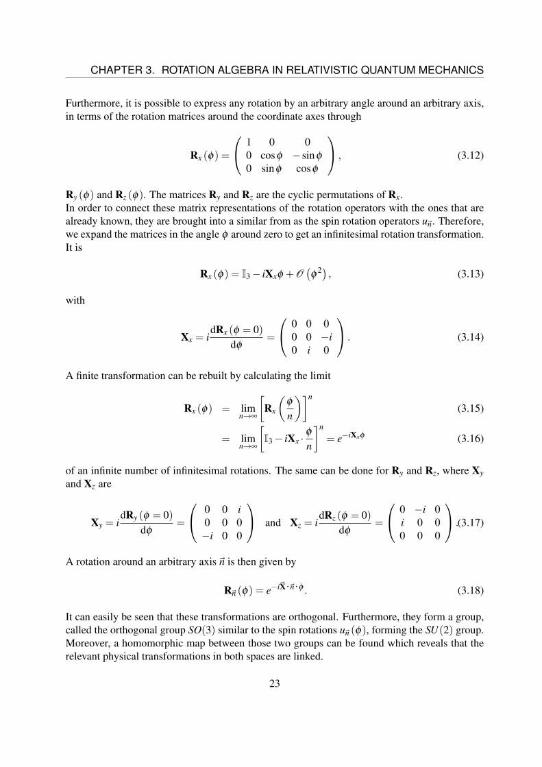
Furthermore, it is possible to express any rotation by an arbitrary angle around an arbitrary axis,in terms of the rotation matrices around the coordinate axes through
Rx (φ) =
1 0 00 cosφ −sinφ
0 sinφ cosφ
, (3.12)
Ry (φ) and Rz (φ). The matrices Ry and Rz are the cyclic permutations of Rx.In order to connect these matrix representations of the rotation operators with the ones that arealready known, they are brought into a similar from as the spin rotation operators u~n. Therefore,we expand the matrices in the angle φ around zero to get an infinitesimal rotation transformation.It is
Rx (φ) = I3− iXxφ +O(φ
2) , (3.13)
with
Xx = idRx (φ = 0)
dφ=
0 0 00 0 −i0 i 0
. (3.14)
A finite transformation can be rebuilt by calculating the limit
Rx (φ) = limn→∞
[Rx
(φ
n
)]n
(3.15)
= limn→∞
[I3− iXx ·
φ
n
]n
= e−iXxφ (3.16)
of an infinite number of infinitesimal rotations. The same can be done for Ry and Rz, where Xyand Xz are
Xy = idRy (φ = 0)
dφ=
0 0 i0 0 0−i 0 0
and Xz = idRz (φ = 0)
dφ=
0 −i 0i 0 00 0 0
.(3.17)
A rotation around an arbitrary axis~n is then given by
R~n (φ) = e−i~X ·~n ·φ . (3.18)
It can easily be seen that these transformations are orthogonal. Furthermore, they form a group,called the orthogonal group SO(3) similar to the spin rotations u~n (φ), forming the SU(2) group.Moreover, a homomorphic map between those two groups can be found which reveals that therelevant physical transformations in both spaces are linked.
23
CHAPTER 3. ROTATION ALGEBRA IN RELATIVISTIC QUANTUM MECHANICS
3.3 Rotation Transformations of OperatorsUp to this point the form of the relevant spatial and spin rotation transformations has been dis-cussed. This chapter will examine how these transformations affect operators.Therefore, an arbitrary rotation operation ω and a wave function ψ are chosen. Applying ω tothe wave function leads to the transformed wave function
ψ′ = ωψ. (3.19)
Now, the same transformation ω is applied to a product of the wave function ψ and an arbitraryoperator O
Oψ = ω−1
ω (Oψ) = ω−1 (O′ωψ
). (3.20)
Obviously the transformed operator has the form
O′ = ωOω−1. (3.21)
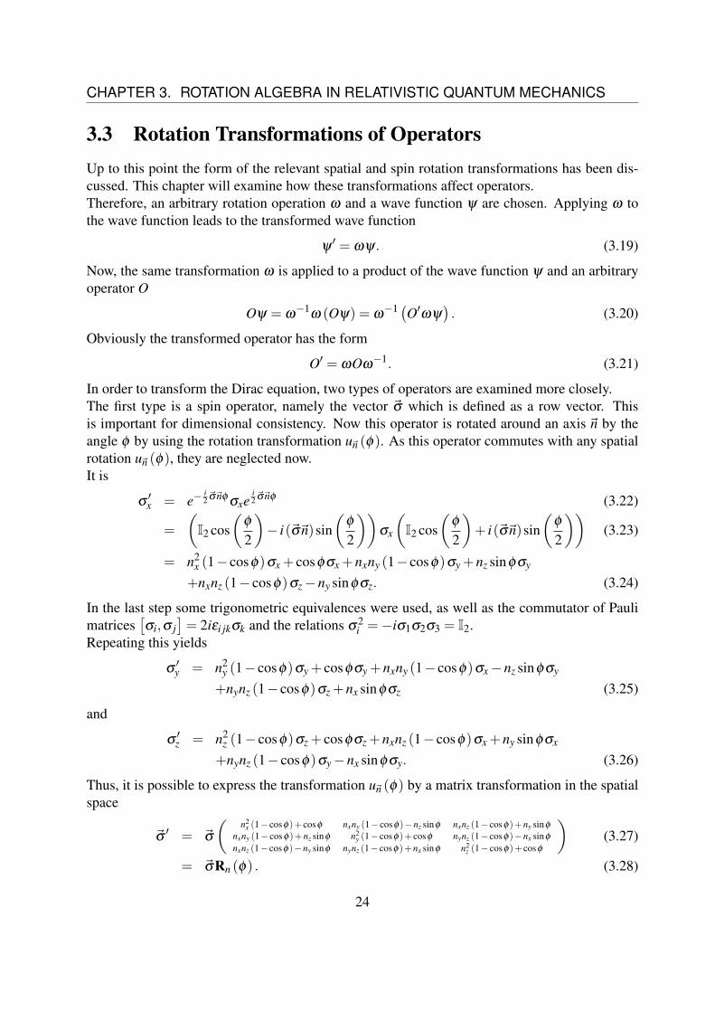
In order to transform the Dirac equation, two types of operators are examined more closely.The first type is a spin operator, namely the vector ~σ which is defined as a row vector. Thisis important for dimensional consistency. Now this operator is rotated around an axis ~n by theangle φ by using the rotation transformation u~n (φ). As this operator commutes with any spatialrotation u~n (φ), they are neglected now.It is
σ′x = e−
i2~σ~nφ
σxei2~σ~nφ (3.22)
=
(I2 cos
(φ
2
)− i(~σ~n)sin
(φ
2
))σx
(I2 cos
(φ
2
)+ i(~σ~n)sin
(φ
2
))(3.23)
= n2x (1− cosφ)σx + cosφσx +nxny (1− cosφ)σy +nz sinφσy
+nxnz (1− cosφ)σz−ny sinφσz. (3.24)
In the last step some trigonometric equivalences were used, as well as the commutator of Paulimatrices
[σi,σ j
]= 2iεi jkσk and the relations σ2
i =−iσ1σ2σ3 = I2.Repeating this yields
σ′y = n2
y (1− cosφ)σy + cosφσy +nxny (1− cosφ)σx−nz sinφσy
+nynz (1− cosφ)σz +nx sinφσz (3.25)
and
σ′z = n2
z (1− cosφ)σz + cosφσz +nxnz (1− cosφ)σx +ny sinφσx
+nynz (1− cosφ)σy−nx sinφσy. (3.26)
Thus, it is possible to express the transformation u~n (φ) by a matrix transformation in the spatialspace
~σ ′ = ~σ
(n2
x (1− cosφ)+ cosφ nxny (1− cosφ)−nz sinφ nxnz (1− cosφ)+ny sinφ
nxny (1− cosφ)+nz sinφ n2y (1− cosφ)+ cosφ nynz (1− cosφ)−nx sinφ
nxnz (1− cosφ)−ny sinφ nynz (1− cosφ)+nx sinφ n2z (1− cosφ)+ cosφ
)(3.27)
= ~σRn (φ) . (3.28)
24
CHAPTER 3. ROTATION ALGEBRA IN RELATIVISTIC QUANTUM MECHANICS
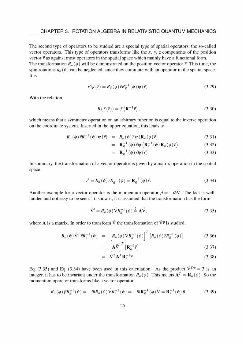
The second type of operators to be studied are a special type of spatial operators, the so-calledvector operators. This type of operators transforms like the x, y, z components of the positionvector~r as against most operators in the spatial space which mainly have a functional form.The transformation R~n (φ) will be demonstrated on the position vector operator~r. This time, thespin rotations u~n (φ) can be neglected, since they commute with an operator in the spatial space.It is
~r′ψ (~r) = R~n (φ)~rR−1~n (φ)ψ (~r) . (3.29)
With the relation
R( f (~r)) = f(R−1~r
), (3.30)
which means that a symmetry operation on an arbitrary function is equal to the inverse operationon the coordinate system. Inserted in the upper equation, this leads to
R~n (φ)~rR−1~n (φ)ψ (~r) = R~n (φ)~rψ (R~n (φ)~r) (3.31)
= R−1~n (φ)~rψ
(R−1~n (φ)R~n (φ)~r
)(3.32)
= R−1~n (φ)~rψ (~r) . (3.33)
In summary, the transformation of a vector operator is given by a matrix operation in the spatialspace
~r′ = R~n (φ)~rR−1~n (φ) = R−1
~n (φ)~r. (3.34)
Another example for a vector operator is the momentum operator ~p = −ih~∇. The fact is well-hidden and not easy to be seen. To show it, it is assumed that the transformation has the form
~∇′ = R~n (φ)~∇R−1~n (φ)
!= A~∇, (3.35)
where A is a matrix. In order to transform ~∇ the transformation of ~∇~r is studied,
R~n (φ)~∇T~rR−1
~n (φ) =[R~n (φ)~∇R−1
~n (φ)]T [
R~n (φ)~rR−1~n (φ)
](3.36)
=[A~∇]T [
R−1~n ~r]
(3.37)
= ~∇T AT R−1~n ~r. (3.38)
Eq. (3.35) and Eq. (3.34) have been used in this calculation. As the product ~∇T~r = 3 is aninteger, it has to be invariant under the transformation R~n (φ). This means AT = R~n (φ). So themomentum operator transforms like a vector operator
R~n (φ)~pR−1~n (φ) =−ihR~n (φ)~∇R−1
~n (φ) =−ihR−1~n (φ)~∇ = R−1
~n (φ)~p. (3.39)
25
CHAPTER 3. ROTATION ALGEBRA IN RELATIVISTIC QUANTUM MECHANICS
3.4 Transformation of the Dirac EquationFinally, the whole Dirac equation
HDψ = c(~α ·~p)ψ +(βmc2 +V
)ψ = Eψ, (3.40)
will be transformed involving the tools acquired in the previous chapters.For the calculation a time independent Hamilton operator with a static scalar potential V is used.For simplification purposes, it is additionally assumed that this potential is spherically symmetric.As it was shown, an arbitrary rotation transformation is an element of the group SU(2)⊗SO(3),which is of the form u~n1 (φ1)⊗R~n2 (φ2)≡ u~n1 (φ1)R~n2 (φ2).The transformed Hamiltonian has the following form:
(HD)′ = u~n1 (φ1)R~n2 (φ2) HD R−1
~n2(φ2)u−1
~n1(φ1) . (3.41)
For energy conservation reasons of the system it is demanded that the Hamiltonian has to beinvariant under the previous transformation, thus
H ′D
!= HD (3.42)
must hold. Since the potential V is both spin independent and spherically symmetric this term istrivially invariant under the rotation transformation. The operator β only takes effect on the spinpart of a wave function, so it is invariant under the spatial rotation, too. Thus it is only necessaryto discuss the effect of the spin part of the transformation on the operator β
u~n1 (φ1)βu−1~n1
(φ1) = u~n1 (φ1)
(I2 0202 −I2
)u−1~n1
(φ1) = β . (3.43)
It can be seen that this operator is trivially invariant under these kind of transformations.Finally we have to study the last part of the Hamiltonian ~α ·~p, which connects the spatial partand the spin part of the system. It is found that
(~α ·~p)′ = u~n1 (φ1)R~n2 (φ2) [~α ·~p] R−1~n2
(φ2)u−1~n1
(φ1) (3.44)
=[u~n1 (φ1) ~α u−1
~n1(φ1)
]·[R~n2 (φ2) ~p R−1
~n2(φ2)
]. (3.45)
For analyzing this term, it will be split into two parts.In the beginning, the focus will be on the spin part u~n1 (φ1) ~α u−1
~n1(φ1), by contemplating the
single components of ~α , with i = x, y, z first. It is
u~n1 (φ1)αiu−1~n1
(φ1) = u~n1 (φ1)
(σi 0202 σi
)u−1~n1
(φ1) . (3.46)
Using Eq. (3.28) it can be easily found that
u~n1 (φ1)~αu−1~n1
(φ1) = ~αR~n1 (φ1) . (3.47)
26
CHAPTER 3. ROTATION ALGEBRA IN RELATIVISTIC QUANTUM MECHANICS
The second part is the transformation of the momentum operator ~p, which has been shown inEq. (3.39).Putting both together, yields the condition
(~α ·~p)′ =[~αR~n1 (φ1)
][R−1~n2
(φ2)~p]= ~α
[R~n1 (φ1)R−1
~n2(φ2)
]~p != ~α ·~p (3.48)
for invariance. This if fulfilled if, and only if
~n1 = ~n2 (3.49)φ1 = φ2. (3.50)
This eventually reveals that rotation transformations of the form
ω~n (φ) = u~n (φ)R~n (φ) (3.51)
leave the Dirac equation invariant. Since the Dirac equation has been used in the Born-Oppenheimerapproximation
H = ∑i
[σ0h0 (i)+~σ ·~hSO (i)
]+Vee +VNN, (3.52)
where h0 (i) =−12~∇T~∇−VNe, this case has to be discussed again.
Most terms are trivially invariant under the rotation transformation. The only issues can appear inthe nucleus-electron potential VNe and the nucleus-nucleus potential VNN. So the rotation axes~nand angles φ have to be restricted to those, who leave these terms invariant. As the wave functionof single atoms should be rotated in the following, VNN becomes zero and the nucleus-electronpotential VNe becomes spherically symmetric and hence invariant under rotation transformations.Thus there are no further restrictions to the rotation transformations that have to be considered.
3.5 Transformation of OrbitalsIn Turbomole, the DFT calculation code we used for our calculations, the molecular orbitalsare written in terms of the spherical harmonic basis. This means that the matrix form of a rotationoperation R in the spatial space for that special basis must be found.As mentioned earlier, it is
ψ′ (~r′)= Rψ
(~r′)= ψ (~r) (3.53)
if~r′ = R~r. That means
Rψ (~r) = ψ(R−1~r
)= ψ
(RT~r
), (3.54)
where the orthogonality R−1 = RT of spatial rotations was used.The matrix form of an arbitrary rotation transformation R is represented in the standard basis byR
R =
Rxx Rxy RxzRyx Ryy RyzRzx Rzy Rzz
. (3.55)
27
CHAPTER 3. ROTATION ALGEBRA IN RELATIVISTIC QUANTUM MECHANICS
The spherical harmonic basis functions for s, p, d, f , etc. orbitals form in each case a basis withthe cardinal number 2l + 1 for the corresponding angular momentum l. Since the 2l + 1 basisfunctions span an invariant subspace, it is possible to write the rotation with an arbitrary basisfunction ψmul (~r) with µ ∈ 1, . . .2l +1 holds
ψlµ
(~r′)= ψ
lµ
(RT~r
)=
2l+1
∑ν=1
ψlν (~r)Dl
νµ (R) , (3.56)
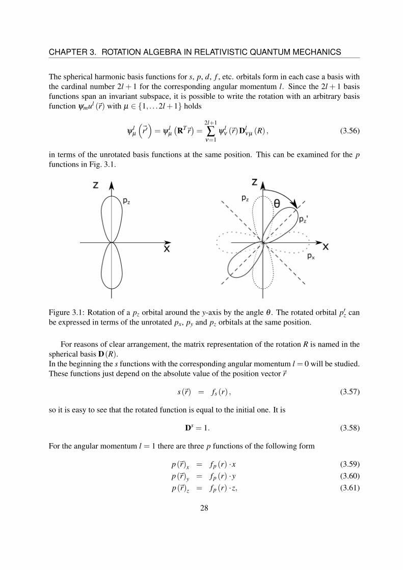
in terms of the unrotated basis functions at the same position. This can be examined for the pfunctions in Fig. 3.1.
Figure 3.1: Rotation of a pz orbital around the y-axis by the angle θ . The rotated orbital p′z canbe expressed in terms of the unrotated px, py and pz orbitals at the same position.
For reasons of clear arrangement, the matrix representation of the rotation R is named in thespherical basis D(R).In the beginning the s functions with the corresponding angular momentum l = 0 will be studied.These functions just depend on the absolute value of the position vector~r
s(~r) = fs (r) , (3.57)
so it is easy to see that the rotated function is equal to the initial one. It is
Ds = 1. (3.58)
For the angular momentum l = 1 there are three p functions of the following form
p(~r)x = fp (r) ·x (3.59)p(~r)y = fp (r) ·y (3.60)p(~r)z = fp (r) ·z, (3.61)
28
CHAPTER 3. ROTATION ALGEBRA IN RELATIVISTIC QUANTUM MECHANICS
where fp (r) is only dependent on the radius r. Using Eq. (3.56), yields
Dp = R (3.62)
for the transformations. This means that the p orbitals transform in the same way as the spatialspace itself.The spherical basis for the d functions (angular momentum l = 2) is
d (~r)3z2−r2 = fd (r) ·3z2− r2
2√
3(3.63)
d (~r)xz = fd (r) ·xz (3.64)d (~r)yz = fd (r) ·yz (3.65)d (~r)xy = fd (r) ·xy (3.66)
d (~r)x2−y2 = fd (r) ·x2− y2
2. (3.67)
By using Eq. (3.56) again, the representation of the rotation for the d function can be found.It is
Dd =
(3R2
zz−1)/2
√3RzxRzz
√3RzyRzz
√3RzxRzy
√3(R2
zx−R2zy/2)
√3RxzRzz RxxRzz +RzxRxz RxyRzz +RxzRzy RxxRzy +RxyRzx RxxRzx−RxyRzy√3RyzRzz RyxRzz +RzxRyz RyyRzz +RyzRzy RyxRzy +RyyRzx RyxRzx−RyyRzy√3RxzRyz RxxRyz +RyxRyz RxyRyz +RyyRxz RxxRyy +RxyRyx RxxRyx−RxyRyy√
3(R2
xzR2yz)/2 RxxRxz−RyxRyz RxyRxz−RyyRyz RxxRxy−RyxRyy
(R2
xx +R2yy−R2
xy−R2yx)/2
. (3.68)
Repetition shows for the f functions (l = 3)
f (~r)2z2−3x2z−3y2z = f f (r) ·2z2−3x2z−3y2z
2√
15(3.69)
f (~r)−x3−xy2+4xz2 = f f (r) ·−x3− xy2 +4xz2
2√
10(3.70)
f (~r)−y3−x2y+4yz2 = f f (r) ·−y3− x2y+4yz2
2√
10(3.71)
f (~r)xyz = f f (r) ·xyz (3.72)
f (~r)x2z−y2z = f f (r) ·x2z− y2z
2(3.73)
f (~r)x3−3xy2 = f f (r) ·x3−3xy2
2√
6(3.74)
f (~r)y3−3x2y = f f (r) ·y3−3x2y
2√
6(3.75)
the obtained rotation’s representation for the spherical harmonics basis D f =(
D f1 ,D
f2 ,D
f3 ,D
f4 ,D
f5 ,D
f6 ,D
f7
)29

CHAPTER 3. ROTATION ALGEBRA IN RELATIVISTIC QUANTUM MECHANICS
with the vector components
D f1 =
(5R3
zz−3Rzz)/2√
6(5RxzR2
zz−Rxz)/4√
6(5RyzR2
zz−Ryz)/4√
15(RxzRyzRzz)√15(R2
xzRzz−R2yzRzz
)/2√
10(R3
xz−3RxzR2yz)/4√
10(R3
yz−3R2xzRyz
)/4
, D f
2 =
√6(5RzxR2
zz−Rzx)/4(
5RxxR2zz−Rxx +10RxzRzxRzz
)/4(
5RyxR2zz−Ryx +10RyzRzxRzz
)/4√
10(RxzRyzRzx +RxzRyxRzz +RxxRyzRzz)/2√10(R2
xzRzx−R2yzRzx +2RxxRxzRzz−2RyxRyzRzz
)/4√
15(RxxR2
xz−RxxR2yz−2RxzRyxRyz
)/4√
15(RyxR2
yz−R2xzRyx−2RxxRxzRyz
)/4
(3.76)
D f3 =
√6(5RzyR2
zz−Rzy)/4(
5RxyR2zz−Rxy +10RxzRzyRzz
)/4(
5RyyR2zz−Ryy +10RyzRzyRzz
)/4√
10(RxyRyzRzz +RxzRyyRzz +RxzRyzRzy)/2√10(R2
xzRzy−R2yzRzy +2RxyRxzRzz−2RyyRyzRzz
)/4√
6(RxxRxyRxz−RxzRyxRyy−RxyRyxRyz−RxxRyyRyz)/2√15(RyyR2
yz−R2xzRyy−2RxyRxzRyz
)/4
, (3.77)
D f4 =
√15(RzxRzyRzz)√
10(RxzRzxRzy +RxyRzxRzz +RxxRzyRzz)/2√10(RyxRzyRzz +RyyRzxRzz +RyzRzxRzy)/2
RxzRyyRzx +RxyRyzRzx +RxzRyxRzy +RxxRyzRzy +RxyRyxRzz +RxxRyyRzzRxyRxzRzx−RyyRyzRzx +RxxRxzRzy−RyxRyzRzy +RxxRxyRzz−RyxRyyRzz√
6(RxxRxyRxz−RxzRyxRyy−RxyRyxRyz−RxxRyyRyz)/2√6(RyxRyyRyz−RxyRxzRyx−RxxRxzRyy−RxxRxyRyz)/2
, (3.78)
D f5 =
√15(R2
zxRzz−R2zyRzz
)/2√
10(RxzR2
zx−R2xzRzy +2RxxRzxRzz−2RxyRzyRzz
)/4√
10(RyzR2
zx−RyzR2zy +2RyxRzxRzz−2RyyRzyRzz
)/4
RxzRyxRzx−RxzRyyRzy +RxxRyzRzx−RxyRyzRzy +RxxRyxRzz−RxyRyyRzz(3RxxRxzRzx−3RxyRxzRzy +RyyRyzRzy−RyxRyzRzx)/2√
6(R2
xxRxz +RxzR2yy−R2
xyRxz−RxzR2yx +2RxyRyyRyz−2RxxRyxRyz
)/4√
6(R2
yxRyz +R2xyRyz−R2
yyRyz−R2xxRyz +2RxyRxzRyy−2RxxRxzRyx
)/4
, (3.79)
D f6 =
√10(R3
zx−3RzxR2zy)/4√
15(RxxR2
zx−RxxR2zy−2RxyRzxRzy
)/4√
15(RyxR2
zx−RyxR2zy−2RyyRzxRzy
)/4√
6(RxxRyxRzx−RxyRyyRzx−RxyRyxRzy−RxxRyyRzy)/2√6(R2
xxRzx +R2yyRzx−R2
yxRzx−R2xyRzx +2RyxRyyRzy−2RxxRxyRzy
)/4(
R3xx +3RxxR2
yy−3RxxR2xy−3RxxR2
yx +6RxyRyxRyy)/4(
R3yx +3R2
xyRyx−3R2xxRyx−3RyxR2
yy +6RxxRxyRyy)/4
(3.80)
and (3.81)
D f7 =
√10(R3
zy−3R2zxRzy
)/4√
15(RxyR2
zy−RxyR2zx−2RxxRzxRzy
)/4√
15(RyyR2
zy−RyyR2zx−2RyxRzxRzy
)/4√
6(RxyRyyRzy−RxyRyxRzx−RxxRyyRzx−RxxRyxRzy)/2√6(R2
xyRzy +R2yxRzy−R2
yyRzy−R2xxRzy +2RyxRyyRzx−2RxxRxyRzx
)/4(
R3xy +3RxyR2
yx−3R2xxRxy−3RxyR2
yy +6RxxRyxRyy)/4(
R3yy +3R2
xxRyy−3R2xyRyy−3R2
yxRyy +6RxxRxyRyx)/4
. (3.82)
This can be done for all higher angular momentums in the same way, but as only the previousbases are necessary for the following calculations this will not be done here.For implementation in Turbomole, it is important to mention that the used basis functions areordered by their angular momentum, this means first the s functions, followed by the p functionsand so on.
30
Chapter 4
The Systems
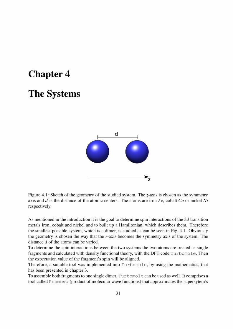
Figure 4.1: Sketch of the geometry of the studied system. The z-axis is chosen as the symmetryaxis and d is the distance of the atomic centers. The atoms are iron Fe, cobalt Co or nickel Nirespectively.
As mentioned in the introduction it is the goal to determine spin interactions of the 3d transitionmetals iron, cobalt and nickel and to built up a Hamiltonian, which describes them. Thereforethe smallest possible system, which is a dimer, is studied as can be seen in Fig. 4.1. Obviouslythe geometry is chosen the way that the z-axis becomes the symmetry axis of the system. Thedistance d of the atoms can be varied.To determine the spin interactions between the two systems the two atoms are treated as singlefragments and calculated with density functional theory, with the DFT code Turbomole. Thenthe expectation value of the fragment’s spin will be aligned.Therefore, a suitable tool was implemented into Turbomole, by using the mathematics, thathas been presented in chapter 3.To assemble both fragments to one single dimer, Turbomole can be used as well. It comprises atool called Promowa (product of molecular wave functions) that approximates the supersytem’s
31

CHAPTER 4. THE SYSTEMS
wave function (dimer) by using the product wave function of the different fragment’s wave func-tions and uses it as starting point for the ensuing self consistent DFT calculations (cf. [Turb70]).These calculations base on energy decomposition analysis [Su09].The whole energy
∆E = Esupermolecule−Efragment = ∆Eelec +∆EXC +∆Erep +∆Epol +∆Edisp (4.1)
between the subsystems is the sum of different energy contributions, containing the electrostaticinteraction ∆Eelec, the exchange interaction ∆EXC, including the spin interactions, the repulsionenergy ∆Erep, that results from the fact, that the wave function of the single fragments are notorthogonal to each other, the dispersion energy ∆Edisp and the polarization energy ∆Epol thatoccurs due to adjustments of the subsystems to each other (e.g. orbital relaxation).A more detailed definition of these energies can be found in [Su09].For our studies the exchange energy
∆EXC = EΩXC
[Mω
∑ω
ρω
]−
Mω
∑ω
EXC [ρω ] (4.2)
between the two subsystems is important as it includes all spin interactions. In this definition Ω
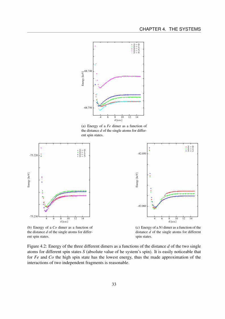
denotes the supersystem and ω the Mω subsystems.The ∆EXC does not only include spin interaction energies, but also e.g. Coulomb interactionslike electron-electron interactions, which do not depend on the spin direction. The energy ∆EXCcan be extracted from the first DFT iteration step after building the product wave function.In all of the calculations the supersystem is always in a high spin state, as it is the ground state ofthe fragments. Therefore, we have to check if this high spin state is the ground state of the dimeras well.In Fig. 4.2 the total energy of the dimer as a function of the distance d of the two single atomsfor different spin states is shown. It can be seen that for Fe and Co the high spin state is theground state. Thus for these elements the approximation of the product wave function is justified,differently to Ni, where the S = 1 state is the ground state. Unfortunately this state cannot beapproximated by a product wave function, as it is no high spin state.
32
CHAPTER 4. THE SYSTEMS
-68.750
-68.740
4 6 8 10 12 14
Ene
rgy
[keV
]
d [a.u.]
S = 0S = 1S = 2S = 3S = 4
(a) Energy of a Fe dimer as a function ofthe distance d of the single atoms for differ-ent spin states.
-75.230
-75.220
4 6 8 10 12 14
Ene
rgy
[keV
]
d [a.u.]
S = 0S = 1S = 2S = 3
(b) Energy of a Co dimer as a function ofthe distance d of the single atoms for differ-ent spin states.
-82.060
-82.050
4 6 8 10 12 14
Ene
rgy
[keV
]
d [a.u.]
S = 0S = 1S = 2
(c) Energy of a Ni dimer as a function of thedistance d of the single atoms for differentspin states.
Figure 4.2: Energy of the three different dimers as a functions of the distance d of the two singleatoms for different spin states S (absolute value of he system’s spin). It is easily noticeable thatfor Fe and Co the high spin state has the lowest energy, thus the made approximation of theinteractions of two independent fragments is reasonable.
33

CHAPTER 4. THE SYSTEMS
34
Chapter 5
Results
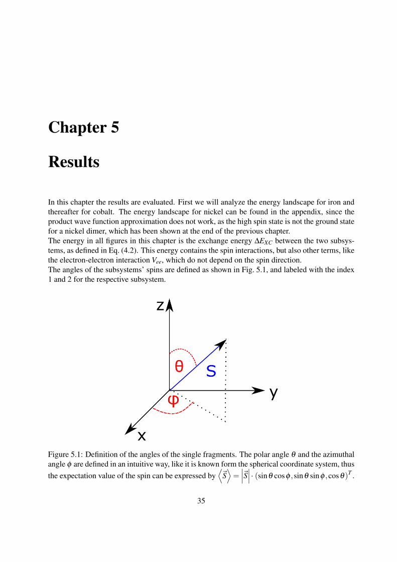
In this chapter the results are evaluated. First we will analyze the energy landscape for iron andthereafter for cobalt. The energy landscape for nickel can be found in the appendix, since theproduct wave function approximation does not work, as the high spin state is not the ground statefor a nickel dimer, which has been shown at the end of the previous chapter.The energy in all figures in this chapter is the exchange energy ∆EXC between the two subsys-tems, as defined in Eq. (4.2). This energy contains the spin interactions, but also other terms, likethe electron-electron interaction Vee, which do not depend on the spin direction.The angles of the subsystems’ spins are defined as shown in Fig. 5.1, and labeled with the index1 and 2 for the respective subsystem.
Figure 5.1: Definition of the angles of the single fragments. The polar angle θ and the azimuthalangle φ are defined in an intuitive way, like it is known form the spherical coordinate system, thusthe expectation value of the spin can be expressed by
⟨~S⟩=∣∣∣~S∣∣∣ · (sinθ cosφ ,sinθ sinφ ,cosθ)T .
35

CHAPTER 5. RESULTS
For the whole energy landscape there are five degrees of freedom. The angles θ1, θ2, φ1 andφ2 for the two subsystem’s spins and the distance d between them.It is necessary to mention that all statements that are made on the spin Hamiltonian are madefrom a semi-classical point of view. Since in the relativistic case the spin is not conserved, itis possible to make statements only on its expectation value. This means if in the followingstatements about spins are made, it is always meant to be the expectation value of the spin, evenif it is not mentioned explicitly.
5.1 IronIt will be shown that the spin-interaction Hamiltonian has the form
Hspin =−D(d)(~r12
(~S1 +~S2
))︸ ︷︷ ︸
Huni
−C(d)(~S1~S2−
(~S1~r12
)(~S2~r12
))︸ ︷︷ ︸
Hdip
−J(d)~S1~S2︸ ︷︷ ︸Hsp
, (5.1)
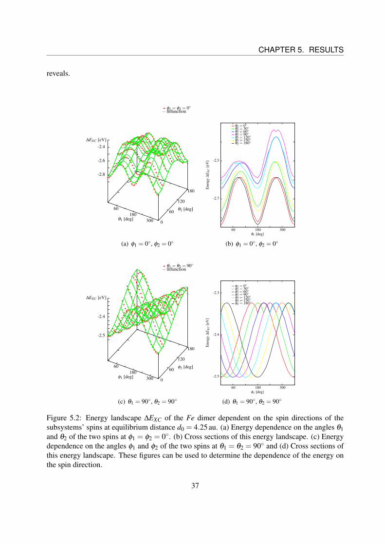
where~r12 is the unity vector between the two spins and thereby the symmetry axis of the system.It is ~r12 = (0,0,1)T = ez.Furthermore, it will be computed a distance dependence of the coefficients and the different partsof the Hamiltonian will be discussed.But first the focus is set on the shape of the energy landscape. In Fig. 5.2 there is ∆EXC shown,as defined in Eq. (4.2), for different angles at the distance of equilibrium d0 = 4.25 au for Fe.In Fig. 5.2 (a) the energy dependence on the angles θ1 and θ2 of the two spins is shown atφ1 = φ2 = 0. Fig. 5.2 (b) shows cross sections of the energy landscape in (a).From the two subfigures a huge amount of information about the behavior of the energy can beextracted. The first dependence that can be noticed is an energy contribution of the form
Euni ∝ cos2θ1 + cos2
θ2. (5.2)
This can be clearly extracted out of the shape of the black and red curve and the symmetry of thedimer molecule. The other curves confirm that.Furthermore Fig. 5.2 (b) illustrates that there must be an energy contribution for which holds
Edip,1 ∝ sinθ1 sinθ2. (5.3)
This behavior can be extracted from the fact, that the main peaks are obviously shifting theirheight to each other by the variation of the angle θ2. This shift has the form of a sinus functionand as the dimer is symmetric, the behavior also occurs by varying θ1.In Fig. 5.2 (c) the energy dependence on the angles φ1 and φ2 of the two spins is shown atθ1 = θ2 = 90.Fig. 5.2 (d) shows again cross sections of the energy landscape in (c). The angles θ1 and θ2 arechosen in the way that the sinus functions in Eq. (5.3) is maximized.In this figure the energy contribution with the form
Edip,2 ∝ cos(φ1−φ2) (5.4)
36
CHAPTER 5. RESULTS
reveals.
60180
300 0
60
120
180
-2.8
-2.6
-2.4
φ1 = φ2 = 0fitfunction
θ1 [deg]
θ2 [deg]
∆EXC [eV]
(a) φ1 = 0, φ2 = 0
-2.7
-2.5
60 180 300
Ene
rgy
∆E
XC
[eV
]
θ1 [deg]
θ2 = 0θ2 = 30θ2 = 60θ2 = 90θ2 = 120θ2 = 150θ2 = 180
(b) φ1 = 0, φ2 = 0
60180
300 0
60
120
180
-2.5
-2.4
θ1 = θ2 = 90fitfunction
φ1 [deg]
φ2 [deg]
∆EXC [eV]
(c) θ1 = 90, θ2 = 90
-2.5
-2.4
-2.3
60 180 300
Ene
rgy
∆E
XC
[eV
]
φ1 [deg]
φ2 = 0φ2 = 30φ2 = 60φ2 = 90φ2 = 120φ2 = 150φ2 = 180
(d) θ1 = 90, θ2 = 90
Figure 5.2: Energy landscape ∆EXC of the Fe dimer dependent on the spin directions of thesubsystems’ spins at equilibrium distance d0 = 4.25 au. (a) Energy dependence on the angles θ1and θ2 of the two spins at φ1 = φ2 = 0. (b) Cross sections of this energy landscape. (c) Energydependence on the angles φ1 and φ2 of the two spins at θ1 = θ2 = 90 and (d) Cross sections ofthis energy landscape. These figures can be used to determine the dependence of the energy onthe spin direction.
37
CHAPTER 5. RESULTS
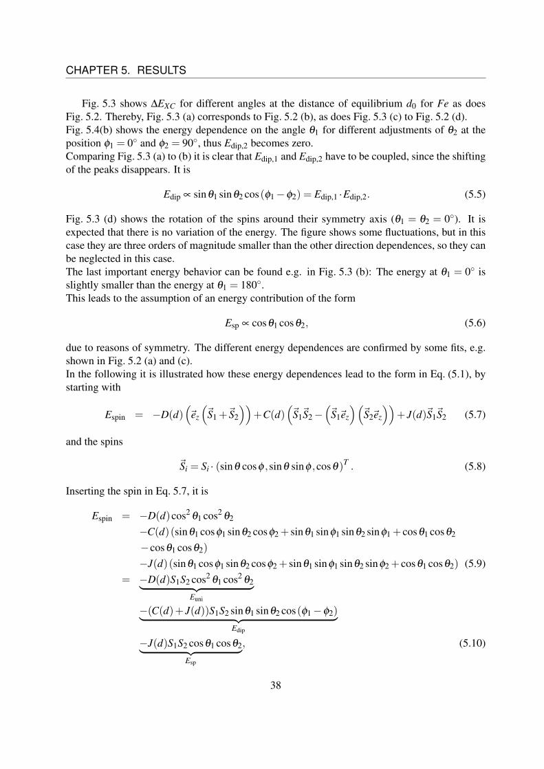
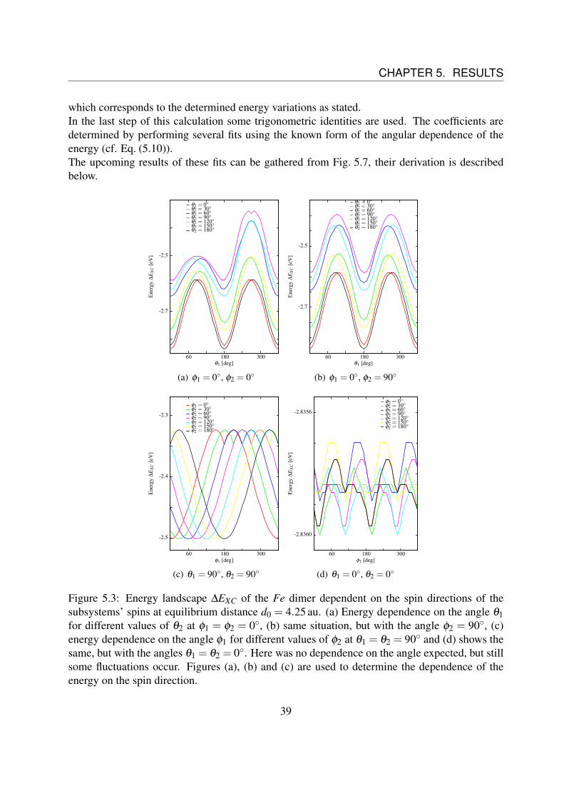
Fig. 5.3 shows ∆EXC for different angles at the distance of equilibrium d0 for Fe as doesFig. 5.2. Thereby, Fig. 5.3 (a) corresponds to Fig. 5.2 (b), as does Fig. 5.3 (c) to Fig. 5.2 (d).Fig. 5.4(b) shows the energy dependence on the angle θ1 for different adjustments of θ2 at theposition φ1 = 0 and φ2 = 90, thus Edip,2 becomes zero.Comparing Fig. 5.3 (a) to (b) it is clear that Edip,1 and Edip,2 have to be coupled, since the shiftingof the peaks disappears. It is
Edip ∝ sinθ1 sinθ2 cos(φ1−φ2) = Edip,1 ·Edip,2. (5.5)
Fig. 5.3 (d) shows the rotation of the spins around their symmetry axis (θ1 = θ2 = 0). It isexpected that there is no variation of the energy. The figure shows some fluctuations, but in thiscase they are three orders of magnitude smaller than the other direction dependences, so they canbe neglected in this case.The last important energy behavior can be found e.g. in Fig. 5.3 (b): The energy at θ1 = 0 isslightly smaller than the energy at θ1 = 180.This leads to the assumption of an energy contribution of the form
Esp ∝ cosθ1 cosθ2, (5.6)
due to reasons of symmetry. The different energy dependences are confirmed by some fits, e.g.shown in Fig. 5.2 (a) and (c).In the following it is illustrated how these energy dependences lead to the form in Eq. (5.1), bystarting with
Espin = −D(d)(~ez
(~S1 +~S2
))+C(d)
(~S1~S2−
(~S1~ez
)(~S2~ez
))+ J(d)~S1~S2 (5.7)
and the spins
~Si = Si · (sinθ cosφ ,sinθ sinφ ,cosθ)T . (5.8)
Inserting the spin in Eq. 5.7, it is
Espin = −D(d)cos2θ1 cos2
θ2
−C(d)(sinθ1 cosφ1 sinθ2 cosφ2 + sinθ1 sinφ1 sinθ2 sinφ1 + cosθ1 cosθ2
−cosθ1 cosθ2)
−J(d)(sinθ1 cosφ1 sinθ2 cosφ2 + sinθ1 sinφ1 sinθ2 sinφ2 + cosθ1 cosθ2) (5.9)= −D(d)S1S2 cos2
θ1 cos2θ2︸ ︷︷ ︸
Euni
−(C(d)+ J(d))S1S2 sinθ1 sinθ2 cos(φ1−φ2)︸ ︷︷ ︸Edip
−J(d)S1S2 cosθ1 cosθ2︸ ︷︷ ︸Esp
, (5.10)
38
CHAPTER 5. RESULTS
which corresponds to the determined energy variations as stated.In the last step of this calculation some trigonometric identities are used. The coefficients aredetermined by performing several fits using the known form of the angular dependence of theenergy (cf. Eq. (5.10)).The upcoming results of these fits can be gathered from Fig. 5.7, their derivation is describedbelow.
-2.7
-2.5
60 180 300
Ene
rgy
∆E
XC
[eV
]
θ1 [deg]
θ2 = 0θ2 = 30θ2 = 60θ2 = 90θ2 = 120θ2 = 150θ2 = 180
(a) φ1 = 0, φ2 = 0
-2.7
-2.5
60 180 300
Ene
rgy
∆E
XC
[eV
]
θ1 [deg]
θ2 = 0θ2 = 30θ2 = 60θ2 = 90θ2 = 120θ2 = 150θ2 = 180
(b) φ1 = 0, φ2 = 90
-2.5
-2.4
-2.3
60 180 300
Ene
rgy
∆E
XC
[eV
]
φ1 [deg]
φ2 = 0φ2 = 30φ2 = 60φ2 = 90φ2 = 120φ2 = 150φ2 = 180
(c) θ1 = 90, θ2 = 90
-2.8360
-2.8356
60 180 300
Ene
rgy
∆E
XC
[eV
]
φ1 [deg]
φ2 = 0φ2 = 30φ2 = 60φ2 = 90φ2 = 120φ2 = 150φ2 = 180
(d) θ1 = 0, θ2 = 0
Figure 5.3: Energy landscape ∆EXC of the Fe dimer dependent on the spin directions of thesubsystems’ spins at equilibrium distance d0 = 4.25 au. (a) Energy dependence on the angle θ1for different values of θ2 at φ1 = φ2 = 0, (b) same situation, but with the angle φ2 = 90, (c)energy dependence on the angle φ1 for different values of φ2 at θ1 = θ2 = 90 and (d) shows thesame, but with the angles θ1 = θ2 = 0. Here was no dependence on the angle expected, but stillsome fluctuations occur. Figures (a), (b) and (c) are used to determine the dependence of theenergy on the spin direction.
39

CHAPTER 5. RESULTS
-2.7
-2.5
60 180 300
Ene
rgy
∆E
XC
[eV
]
θ1 [deg]
θ2 = 0θ2 = 30θ2 = 60θ2 = 90θ2 = 120θ2 = 150θ2 = 180
(a) φ1 = 0, φ2 = 0, d0
-0.042
-0.041
60 180 300
Ene
rgy
∆E
XC
[eV
]
θ1 [deg]
θ2 = 0θ2 = 30θ2 = 60θ2 = 90θ2 = 120θ2 = 150θ2 = 180
(b) φ1 = 0, φ2 = 0, dW
-2.7
-2.5
60 180 300
Ene
rgy
∆E
XC
[eV
]
θ1 [deg]
θ2 = 0θ2 = 30θ2 = 60θ2 = 90θ2 = 120θ2 = 150θ2 = 180
(c) φ1 = 0, φ2 = 90, d0
-0.042
-0.041
60 180 300
Ene
rgy
∆E
XC
[eV
]
θ1 [deg]
θ2 = 0θ2 = 30θ2 = 60θ2 = 90θ2 = 120θ2 = 150θ2 = 180
(d) φ1 = 0, φ2 = 90, dW
-2.5
-2.4
-2.3
60 180 300
Ene
rgy
∆E
XC
[eV
]
φ1 [deg]
φ2 = 0φ2 = 30φ2 = 60φ2 = 90φ2 = 120φ2 = 150φ2 = 180
(e) θ1 = 90, θ2 = 90, d0
-0.042
-0.041
60 180 300
Ene
rgy
∆E
XC
[eV
]
φ1 [deg]
φ2 = 0φ2 = 30φ2 = 60φ2 = 90φ2 = 120φ2 = 150φ2 = 180
(f) θ1 = 90, θ2 = 90, dW
Figure 5.4: Energy landscape ∆EXC of the Fe dimer dependent on the spin directions of thesubsystems’ spins at equilibrium distance d0 = 4.25 au on the left side, consisting of (a), (c), and(e) and at dW = 9.25 au on the right side, consisting of (b), (d) and (f).
40

CHAPTER 5. RESULTS
The next step is to determine the dependence of the coefficients D(d), J(d) and C(d) on thedistance d between the two single atoms. Therefore, we have to do the same analysis for severaldistances d. Fig. 5.4 shows the spin direction dependent energy landscape for the equilibriumdistance d0 = 4.25 au on the left side ((a), (c) and (e)) and for d = 9,25 au on the right side ((b),(d) and (f)) for different spin directions.It can be noticed that the coupling changes from a ferromagnetic state (parallel spins) to a anti-ferromagnetic state (anti-parallel spins), as it can be seen comparing Fig. 5.4 (a) to (b).Furthermore, it can easily be understood that the energy term Esp ∝ cosθ1 cosθ2 becomes strongeras compared to the other terms, as the two main peaks grow together comparing Fig. 5.4 (c) to(d). The behavior in Fig. (f) seems to be strange, but will be explained soon.
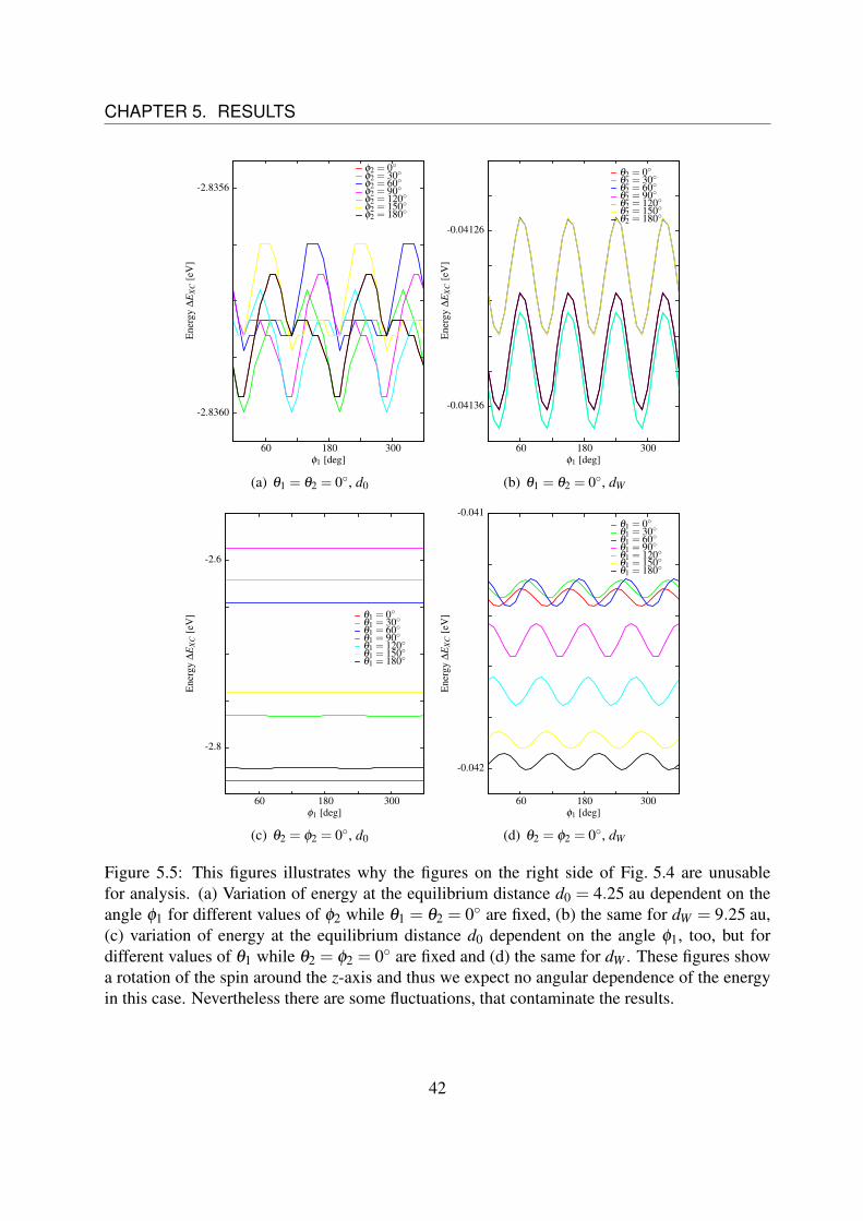
Unfortunately, the figures on the right side of Fig. 5.4 are unusable for analysis, since the fluctu-ations in the energy landscape are at the same magnitude as the variations we want to observe.This can be seen in Fig. 5.5.Fig. 5.5 (a) shows the variation of energy at the equilibrium distance d0 as function of the angleφ1 for different values of φ2 while θ1 = θ2 = 0 are fixed. Fig. 5.5 (c) shows the variation ofenergy at the equilibrium distance d0 = 4,25 au as function of the angle φ1, too, but this time fordifferent values of θ1 while θ2 = φ2 = 0 are fixed.Fig. 5.5 (b) shows the same situation as (a) and Fig. 5.5 (d) shows the same situation as (b) re-spectively, but at a distance of dW = 9.25 au.These figures show a rotation of the spin around the z-axis and thus there are no angular depen-dences of the energy expected in this case. Nevertheless, there are some fluctuations. For theequilibrium distance d0 these fluctuations are very small (three orders of magnitude), comparingthem to the variations of the energy, that should be observed, like in Fig 5.4 (a), (c) and (e),whereas for dW these fluctuations are of the same magnitude as the variations, that should beobserved (cf. Fig 5.4 (b), (d) and (f)).Therefore, it is impossible to differentiate between the fluctuations and the real behavior, whatexplains the weird curve in Fig 5.4 (f).
Here, the problem is that the energy ∆EXC does not only consist of spin interactions, but alsoof Coulomb interactions, like electron-electron interactions as described in chapter 4. The latternormally do not depend on the direction, but as we noticed the total electron density of the singlefragments are not spherically symmetric, as they should. This can be seen in Fig 5.6. It showsthe total density for a single subsystem of Fe (a), Co (b) and Ni (c) for different directions. It isobvious that these densities are not spherical. Thus Coulomb-like interactions become dependenton the direction, too, what makes it impossible to analyze the data for large distances betweenthe fragments.
41
CHAPTER 5. RESULTS
-2.8360
-2.8356
60 180 300
Ene
rgy
∆E
XC
[eV
]
φ1 [deg]
φ2 = 0φ2 = 30φ2 = 60φ2 = 90φ2 = 120φ2 = 150φ2 = 180
(a) θ1 = θ2 = 0, d0
-0.04136
-0.04126
60 180 300E
nerg
y∆
EX
C[e
V]
φ1 [deg]
θ2 = 0θ2 = 30θ2 = 60θ2 = 90θ2 = 120θ2 = 150θ2 = 180
(b) θ1 = θ2 = 0, dW
-2.8
-2.6
60 180 300
Ene
rgy
∆E
XC
[eV
]
φ1 [deg]
θ1 = 0θ1 = 30θ1 = 60θ1 = 90θ1 = 120θ1 = 150θ1 = 180
(c) θ2 = φ2 = 0, d0
-0.042
-0.041
60 180 300
Ene
rgy
∆E
XC
[eV
]
φ1 [deg]
θ1 = 0θ1 = 30θ1 = 60θ1 = 90θ1 = 120θ1 = 150θ1 = 180
(d) θ2 = φ2 = 0, dW
Figure 5.5: This figures illustrates why the figures on the right side of Fig. 5.4 are unusablefor analysis. (a) Variation of energy at the equilibrium distance d0 = 4.25 au dependent on theangle φ1 for different values of φ2 while θ1 = θ2 = 0 are fixed, (b) the same for dW = 9.25 au,(c) variation of energy at the equilibrium distance d0 dependent on the angle φ1, too, but fordifferent values of θ1 while θ2 = φ2 = 0 are fixed and (d) the same for dW . These figures showa rotation of the spin around the z-axis and thus we expect no angular dependence of the energyin this case. Nevertheless there are some fluctuations, that contaminate the results.
42
CHAPTER 5. RESULTS
(a) Total electron denisty of the used Fe fragments in the ground state.
(b) Total electron denisty of the used Co fragments in the ground state.
(c) Total electron denisty of the used Ni fragments in the ground state.
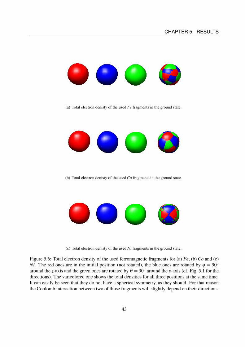
Figure 5.6: Total electron density of the used ferromagnetic fragments for (a) Fe, (b) Co and (c)Ni. The red ones are in the initial position (not rotated), the blue ones are rotated by φ = 90
around the z-axis and the green ones are rotated by θ = 90 around the y-axis (cf. Fig. 5.1 for thedirections). The varicolored one shows the total densities for all three positions at the same time.It can easily be seen that they do not have a spherical symmetry, as they should. For that reasonthe Coulomb interaction between two of those fragments will slightly depend on their directions.
43
CHAPTER 5. RESULTS
Therefore, it is only possible to analyze the data for distances d = 2,5 au to d = 6,1 au. Fitson the data were made, as it can be seen in Fig. 5.2 (a) and (c), by using a fit function of the form
f (θ1,θ2,φ1,φ2) = a · cos2θ1 +b · cos2
θ2
+c · cosθ1 cosθ2 +d · sinθ1 sinθ2 cos(φ1−φ2)+ e. (5.11)
With the help of Eq. (5.10) the fitting-parameters a, b, c and d are assigned to the coefficients D,J and C. The parameter e is an offset that results form the spin-independent terms.The results can be found in Fig. 5.7. Unfortunately it was not possible to detect some interestingresults at the change from a ferromagnetic to a anti-ferromagnetic state, as it happens for largerdistances than analyzed. How these calculations can be improved will be discussed in chapter 6.
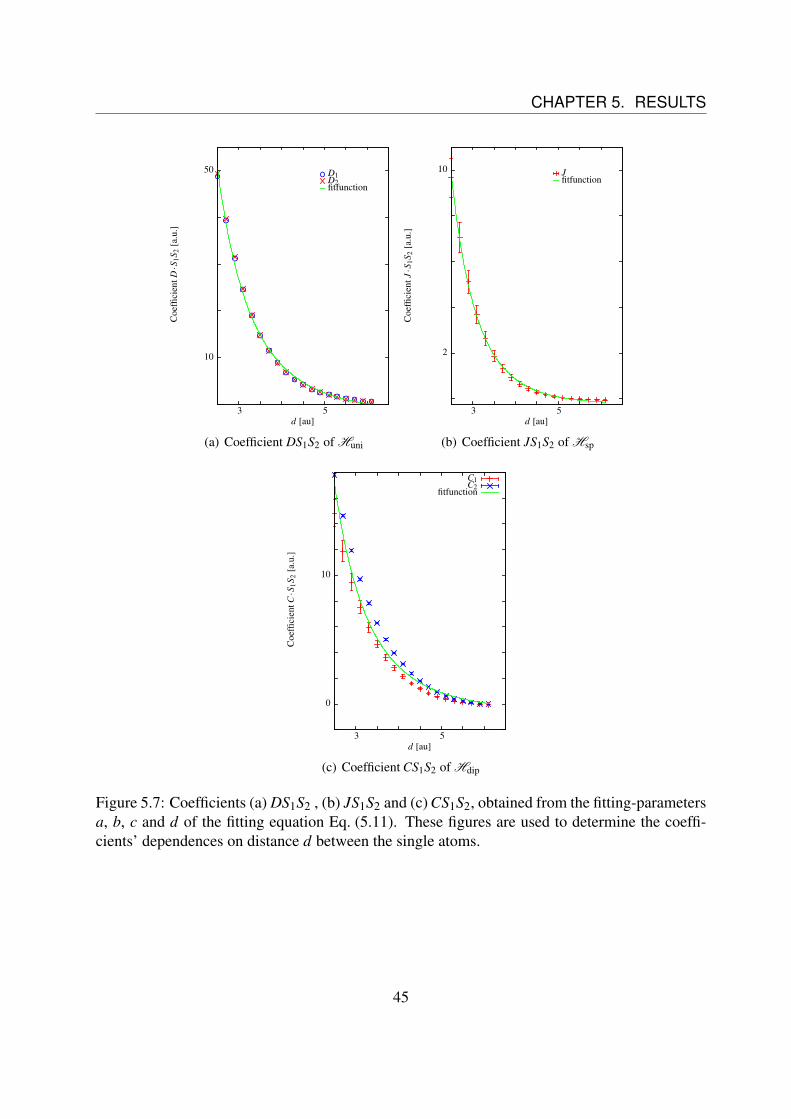
Fig. 5.7 (a) shows the dependence of the coefficient D1/2S1S2 of Huni (c.f. Eq. (5.12)) as afunction of the distance d. Thereby D1 are the values obtained from the fitting-parameter a andD2 the ones from the parameter b respectively. The figure shows a decrease which is proportionalto d−3. This is validated by fitting the values.It was fitted on the function fD(d) = a ·d−3 +b ·d−1. The parameter a is a = D ·S1S2, while theterm with the parameter b approximates the fluctuations that result from the non-spherical totaldensity of the subsystems. The exponents in the fitting function were varied during the fittingprocedure as well, but did not vary appreciably, so they were chosen as being fixed.The results of the fitting can be found in Tab. 5.1.Fig. 5.7 (b) illustrates the dependence of the coefficient JS1S2 of Hsp (c.f. Eq. (5.12)) as functionof the distance d instead. The figure shows a decrease which is proportional to d−4. This isvalidated by fitting the values.It was fitted on the function fJ(d) = a ·d−4 + b ·d−1. The parameter a is a = J ·S1S2, while theterm with the parameter b approximates the fluctuations that result from the non-spherical totaldensity of the subsystems. The exponents in the fitting function were varied during the fittingprocedure as well, but did not vary appreciably, so they were chosen as being fixed.The results of the fitting can be found in Tab. 5.1, again.As last, Fig. 5.7 (c) shows the dependence of the coefficient CS1S2 of Hdip (c.f. Eq. (5.12)) asfunction of the distance. Thereby C1 are the values obtained from the fitting-parameter c, andC2 from the parameter d respectively. The figure shows a decrease which is proportional to d−3.This is validated by fitting the values.Again, it was fitted on fC(d) = a ·d−3 +b ·d−1. The parameter a is a = D ·S1S2, while the termwith the parameter b approximates the fluctuations that result from the non-spherical total den-sity of the subsystems, as before. The exponents in the fitting function were varied during thefitting procedure as well, but did not vary appreciably in this case, too. Thus they were chosenas being fixed.Unfortunately the coefficients resulting from both previous fitting parameters do not agree thatwell, so there must be a larger impact of the fluctuations in the results than expected.The results of the fitting can also be found in Tab. 5.1.
44
CHAPTER 5. RESULTS
10
50
3 5
Coe
ffici
entD
·S1S
2[a
.u.]
d [au]
D1D2fitfunction
(a) Coefficient DS1S2 of Huni
2
10
3 5C
oeffi
cien
tJ·S
1S2
[a.u
.]
d [au]
Jfitfunction
(b) Coefficient JS1S2 of Hsp
0
10
3 5
Coe
ffici
entC
·S1S
2[a
.u.]
d [au]
C1C2fitfunction
(c) Coefficient CS1S2 of Hdip
Figure 5.7: Coefficients (a) DS1S2 , (b) JS1S2 and (c) CS1S2, obtained from the fitting-parametersa, b, c and d of the fitting equation Eq. (5.11). These figures are used to determine the coeffi-cients’ dependences on distance d between the single atoms.
45

CHAPTER 5. RESULTS
Table 5.1: Parameters a and b, obtained from the fitting process over the values in Fig. 5.7. Theuncertainties result from the fitting process.
DS1S2 JS1S2 CS1S2
a [a.u.] 947.01 ± 10.65 429.95 ± 4.54 321.02 ± 11.96b [a.u.] 25.35 ± 1.00 3.15 ± 0.16 8.42 ± 1.18
All in all, the spin dependent energy and hence the spin-dependent Hamiltonian is
Hspin =−Dr3
12
(~r12
(~S1 +~S2
))︸ ︷︷ ︸
Huni
− Cr3
12
(~S1~S2−
(~S1~r12
)(~S2~r12
))︸ ︷︷ ︸
Hdip
− Jr4
12
~S1~S2︸ ︷︷ ︸Hsp
, (5.12)
with the coefficients in Tab. 5.2 and the unity vector ~r12 between the two atoms.
Table 5.2: Coefficents of the Hamiltonian Eq. (5.12), derived with the values in Tab. 5.1 and theabsolute value of the atomic Fe subsystems S1 = S2 = 2.
D [eVa3B] J [eVa4
B] C [eVa3B]
236.75 ± 2.67 107.49 ± 1,13 80.27 ± 2.92
This Hamiltonian contains three terms. The first term is the Heisenberg interaction-like Hsp,which does not show an anisotropy. It only depends on the distance of both atoms. As seen inFig. 5.4 (a) and (b), the full distance dependency is not described by an r−4
12 decrease, since thisenergy contribution becomes larger compared to the other ones at large distances. Furthermore,it occurs a change of sign for that term, as for large distances the anti-ferromagnetic orientationis preferred. That means that the calculations only describe the behavior of this term around thedistance of equilibrium.
The second term Huni is a Dzyaloshinskii-Moriya-like uniaxial spin Hamiltonian, that is char-acteristic for single molecule magnets. This term leads to a magnetic anisotropy and is a strongspin-lattice coupling, that leads to a spin-phonon interaction in the molecule as described in e.g.[Gar15]. Unfortunately, as far as known, there are no distance dependent measurements on thisinteraction, so it cannot be compared with experimental values.
The last term, Hdip, is a magnetic dipolar-dipolar interaction, that is occurring due to spin-latticecoupling. Van Vleck proposed this kind of interaction in 1937 [Vle37], and [Ass] shows that thiskind of spin-lattice coupling already leads to the Einstein-de Haas effect. Thus, due to this spin-lattice inducted dipolar-dipolar interaction an angular momentum is transferred from the spins tothe lattice by adjusting them with a magnetic field or something similar. A Huni-like term wasnot included in the calculations of [Ass].
46
CHAPTER 5. RESULTS
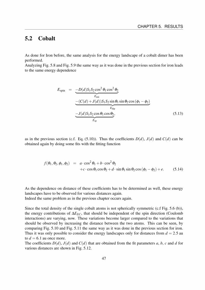
5.2 Cobalt
As done for Iron before, the same analysis for the energy landscape of a cobalt dimer has beenperformed.Analyzing Fig. 5.8 and Fig. 5.9 the same way as it was done in the previous section for iron leadsto the same energy dependence
Espin = −D(d)S1S2 cos2θ1 cos2
θ2︸ ︷︷ ︸Euni
−(C(d)+ J(d))S1S2 sinθ1 sinθ2 cos(φ1−φ2)︸ ︷︷ ︸Edip
−J(d)S1S2 cosθ1 cosθ2︸ ︷︷ ︸Esp
, (5.13)
as in the previous section (c.f. Eq. (5.10)). Thus the coefficients D(d), J(d) and C(d) can beobtained again by doing some fits with the fitting function
f (θ1,θ2,φ1,φ2) = a · cos2θ1 +b · cos2
θ2
+c · cosθ1 cosθ2 +d · sinθ1 sinθ2 cos(φ1−φ2)+ e. (5.14)
As the dependence on distance of these coefficients has to be determined as well, these energylandscapes have to be observed for various distances again.Indeed the same problem as in the previous chapter occurs again.
Since the total density of the single cobalt atoms is not spherically symmetric (c.f Fig. 5.6 (b)),the energy contributions of ∆EXC, that should be independent of the spin direction (Coulombinteractions) are varying, now. These variations become larger compared to the variations thatshould be observed by increasing the distance between the two atoms. This can be seen, bycomparing Fig. 5.10 and Fig. 5.11 the same way as it was done in the previous section for iron.Thus it was only possible to consider the energy landscapes only for distances from d = 2.5 auto d = 6.1 au once more.The coefficients D(d), J(d) and C(d) that are obtained from the fit parameters a, b, c and d forvarious distances are shown in Fig. 5.12.
47
CHAPTER 5. RESULTS
60180
300 0
60
120
180
-4.3
-4.0
-3.7
φ1 = φ2 = 0fitfunction
θ1 [deg]
θ2 [deg]
∆EXC [eV]
(a) φ1 = 0, φ2 = 0
-4.0
-3.8
180 300E
nerg
y∆
EX
C[e
V]
θ1 [deg]
θ2 = 0θ2 = 30θ2 = 60θ2 = 90θ2 = 120θ2 = 150θ2 = 180
(b) φ1 = 0, φ2 = 0
60180
300 0
60
120
180
-3.9
-3.8
θ1 = θ2 = 90fitfunction
φ1 [deg]
φ2 [deg]
∆EXC [eV]
(c) θ1 = 90, θ2 = 90
-3.8
-3.7
60 180 300
Ene
rgy
∆E
XC
[eV
]
φ1 [deg]
φ2 = 0φ2 = 30φ2 = 60φ2 = 90φ2 = 120φ2 = 150φ2 = 180
(d) θ1 = 90, θ2 = 90
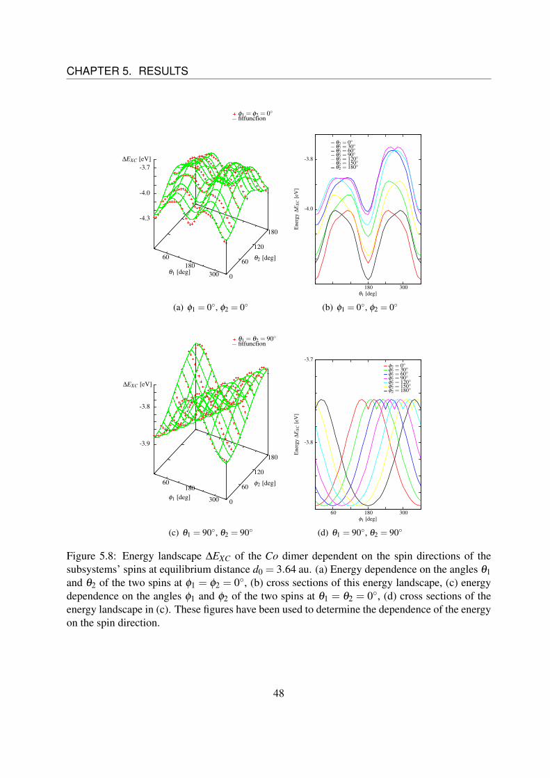
Figure 5.8: Energy landscape ∆EXC of the Co dimer dependent on the spin directions of thesubsystems’ spins at equilibrium distance d0 = 3.64 au. (a) Energy dependence on the angles θ1and θ2 of the two spins at φ1 = φ2 = 0, (b) cross sections of this energy landscape, (c) energydependence on the angles φ1 and φ2 of the two spins at θ1 = θ2 = 0, (d) cross sections of theenergy landscape in (c). These figures have been used to determine the dependence of the energyon the spin direction.
48
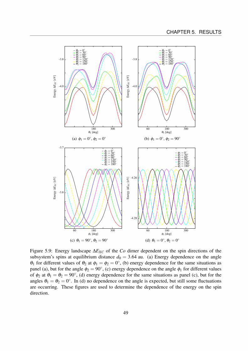
CHAPTER 5. RESULTS
-4.0
-3.8
180 300
Ene
rgy
∆E
XC
[eV
]
θ1 [deg]
θ2 = 0θ2 = 30θ2 = 60θ2 = 90θ2 = 120θ2 = 150θ2 = 180
(a) φ1 = 0, φ2 = 0
-4.0
-3.8
60 180 300E
nerg
y∆
EX
C[e
V]
θ1 [deg]
θ2 = 0θ2 = 30θ2 = 60θ2 = 90θ2 = 120θ2 = 150θ2 = 180
(b) φ1 = 0, φ2 = 90
-3.8
-3.7
60 180 300
Ene
rgy
∆E
XC
[eV
]
φ1 [deg]
φ2 = 0φ2 = 30φ2 = 60φ2 = 90φ2 = 120φ2 = 150φ2 = 180
(c) θ1 = 90, θ2 = 90
-4.28
-4.26
60 180 300
Ene
rgy
∆E
XC
[eV
]
φ1 [deg]
φ2 = 0φ2 = 30φ2 = 60φ2 = 90φ2 = 120φ2 = 150φ2 = 180
(d) θ1 = 0, θ2 = 0
Figure 5.9: Energy landscape ∆EXC of the Co dimer dependent on the spin directions of thesubsystem’s spins at equilibrium distance d0 = 3.64 au. (a) Energy dependence on the angleθ1 for different values of θ2 at φ1 = φ2 = 0, (b) energy dependence for the same situations aspanel (a), but for the angle φ2 = 90, (c) energy dependence on the angle φ1 for different valuesof φ2 at θ1 = θ2 = 90, (d) energy dependence for the same situations as panel (c), but for theangles θ1 = θ2 = 0. In (d) no dependence on the angle is expected, but still some fluctuationsare occurring. These figures are used to determine the dependence of the energy on the spindirection.
49
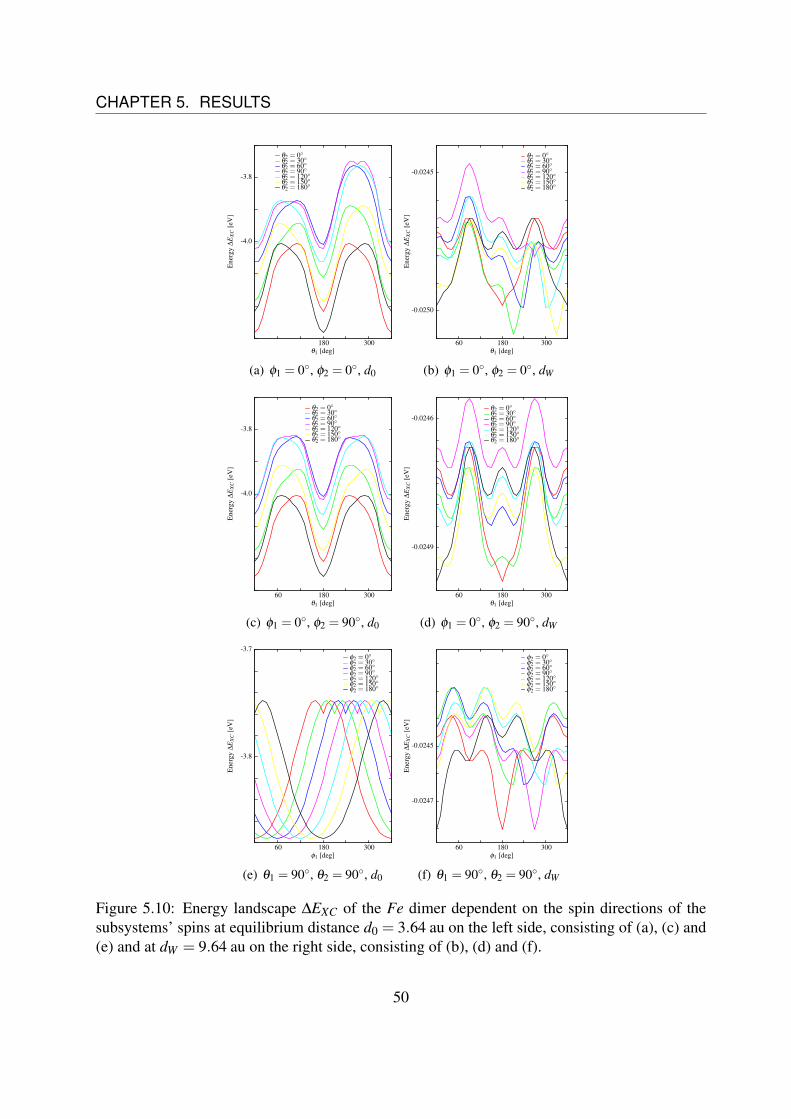
CHAPTER 5. RESULTS
-4.0
-3.8
180 300
Ene
rgy
∆E
XC
[eV
]
θ1 [deg]
θ2 = 0θ2 = 30θ2 = 60θ2 = 90θ2 = 120θ2 = 150θ2 = 180
(a) φ1 = 0, φ2 = 0, d0
-0.0250
-0.0245
60 180 300
Ene
rgy
∆E
XC
[eV
]
θ1 [deg]
θ2 = 0θ2 = 30θ2 = 60θ2 = 90θ2 = 120θ2 = 150θ2 = 180
(b) φ1 = 0, φ2 = 0, dW
-4.0
-3.8
60 180 300
Ene
rgy
∆E
XC
[eV
]
θ1 [deg]
θ2 = 0θ2 = 30θ2 = 60θ2 = 90θ2 = 120θ2 = 150θ2 = 180
(c) φ1 = 0, φ2 = 90, d0
-0.0249
-0.0246
60 180 300
Ene
rgy
∆E
XC
[eV
]
θ1 [deg]
θ2 = 0θ2 = 30θ2 = 60θ2 = 90θ2 = 120θ2 = 150θ2 = 180
(d) φ1 = 0, φ2 = 90, dW
-3.8
-3.7
60 180 300
Ene
rgy
∆E
XC
[eV
]
φ1 [deg]
φ2 = 0φ2 = 30φ2 = 60φ2 = 90φ2 = 120φ2 = 150φ2 = 180
(e) θ1 = 90, θ2 = 90, d0
-0.0247
-0.0245
60 180 300
Ene
rgy
∆E
XC
[eV
]
φ1 [deg]
φ2 = 0φ2 = 30φ2 = 60φ2 = 90φ2 = 120φ2 = 150φ2 = 180
(f) θ1 = 90, θ2 = 90, dW
Figure 5.10: Energy landscape ∆EXC of the Fe dimer dependent on the spin directions of thesubsystems’ spins at equilibrium distance d0 = 3.64 au on the left side, consisting of (a), (c) and(e) and at dW = 9.64 au on the right side, consisting of (b), (d) and (f).
50

CHAPTER 5. RESULTS
-4.28
-4.26
60 180 300
Ene
rgy
∆E
XC
[eV
]
φ1 [deg]
φ2 = 0φ2 = 30φ2 = 60φ2 = 90φ2 = 120φ2 = 150φ2 = 180
(a) θ1 = θ2 = 0, d0 = 4.25 au
-0.0248
-0.0246
60 180 300E
nerg
y∆
EX
C[e
V]
φ1 [deg]
θ2 = 0θ2 = 30θ2 = 60θ2 = 90θ2 = 120θ2 = 150θ2 = 180
(b) θ1 = θ2 = 0, dW = 9.25 au
-4.25
-4.00
60 180 300
Ene
rgy
∆E
XC
[eV
]
φ1 [deg]
θ1 = 0θ1 = 30θ1 = 60θ1 = 90θ1 = 120θ1 = 150θ1 = 180
(c) θ2 = φ2 = 0, d0 = 4.25 au
-0.0250
-0.0245
60 180 300
Ene
rgy
∆E
XC
[eV
]
φ1 [deg]
θ1 = 0θ1 = 30θ1 = 60θ1 = 90θ1 = 120θ1 = 150θ1 = 180
(d) θ2 = φ2 = 0, dW = 9.25 au
Figure 5.11: This figure illustrates why the figures on the right side of Fig. 5.10 are unusable foranalysis. (a) 5.3 Variation of energy at the equilibrium distance d0 = 3.64 au dependent on theangle φ1 for different values of φ2 while θ1 = θ2 = 0 are fixed, (b) the same for dW = 9.64 au,(c) variation of energy at the equilibrium distance d0 dependent on the angle φ1, too, but fordifferent values of θ1 while θ2 = φ2 = 0 are fixed and (d) the same for dW . These figures showa rotation of the spin around the z-axis and thus we expect no angular dependence of the energyin this case. Nevertheless there are some fluctuations, that contaminate the results.
51

CHAPTER 5. RESULTS
0
15
3 5
Fitp
aram
eter
DS 1
S 2[a
.u.]
d [au]
D1D2fitfunction
(a) Coefficient DS1S2 of Huni
1
7
3 5Fi
tpar
amet
erJS
1S2
[a.u
.]
d [au]
Jfitfunction
(b) Coefficient JS1S2 of Hsp
1
8
3 5
Fitp
aram
eter
CS 1
S 2[a
.u.]
d [au]
C2C2fitfunction
(c) Coefficient CS1S2 of Hdip
Figure 5.12: Coefficients (a) DS1S2 , (b) JS1S2 and (c) CS1S2, obtained from the fitting-parameters a, b, c and d of the fitting equation Eq. (5.11). These figures are used to determinethe coefficients’ dependence on distance d of the single atoms
.
Fig. 5.12 (a) shows the dependence of the coefficient D1/2S1S2 of Huni (c.f. Eq. (5.15)) onthe distance d for the calculations for cobalt. Thereby D1 are the values obtained from the fitting-parameter a, and D2 from the parameter b respectively. The figure shows a decrease which isproportional to d−3. This is validated by fitting the values.
52
CHAPTER 5. RESULTS
It was fitted on the function fD(d) = a ·d−3 +b ·d−1. The parameter a is a = D ·S1S2, while theterm with the parameter b approximates the fluctuations that result from the non-spherical totaldensity of the subsystems. The exponents in the fitting function were varied during the fittingprocedure as well, but did not vary appreciably, so they were chosen as being fixed.The results of the fitting can be found in Tab. 5.1.Fig. 5.12 (b) shows the dependence of the coefficient JS1S2 of Hsp (c.f. Eq. (5.15)) on thedistance instead. The figure shows a decrease which is proportional to d−4. This is also validatedby fitting the values.It was fitted on the function fJ(d) = a ·d−4 + b ·d−1. The parameter a is a = J ·S1S2, while theterm with the parameter b approximates the fluctuations that result from the non-spherical totaldensity of the subsystems. The exponents in the fitting function were varied during the fittingprocedure as well but did not vary appreciably, so they were chosen as being fixed again.The results of the fitting can be found in Tab. 5.1.As last, Fig. 5.12 (c) shows the dependence of the coefficient CS1S2 of Hdip (c.f. Eq. (5.15))on the distance d. Like in the previous chapter C1 are the values obtained from the fitting-parameter c, and C2 from the parameter d, respectively. The figure shows a decrease which isproportional to d−3. This is validated by fitting the values. Again, it was fitted on the functionfC(d) = a ·d−3 + b ·d−1. The parameter a is a = D ·S1S2, while the term with the parameter bapproximates the fluctuations that result from the non-spherical total density of the subsystemsagain. The exponents in the fitting function were varied during the fitting procedure as well butdid not vary appreciably, so they were chosen as fixed once again.The results of the fitting can be found in Tab. 5.3.
Table 5.3: Parameters a and b, obtained from the fitting process over the values in Fig. 5.12. Theuncertainties result from the fitting process.
DS1S2 JS1S2 CS1S2
a [a.u.] 346.53 ± 10.65 261.74 ± 4.56 132.94 ± 0.73b [a.u.] 5.80 ± 1.05 0.91 ± 0.16 3.43 ± 0.04
The parameters for the resulting Hamiltonian
Hspin =−Dr3
12
(~r12
(~S1 +~S2
))︸ ︷︷ ︸
Huni
− Cr3
12
(~S1~S2−
(~S1~r12
)(~S2~r12
))︸ ︷︷ ︸
Hdip
− Jr4
12
~S1~S2︸ ︷︷ ︸Hsp
, (5.15)
can be obtained from the fitting-parameters in Tab. 5.3 and are presented in Tab. 5.4.
Table 5.4: Coefficients of the Hamiltonian Eq. (5.12), derived with the values in Tab. 5.3 and theabsolute value of the atomic subsystems S1 = S2 = 1.5.
D [eVa3B] J [eVa4
B] C [eVa3B]
145.01 ± 4.73 116.31 ± 2.03 56.08 ± 0.33
53
CHAPTER 5. RESULTS
It is obvious and not surprising that the resulting Hamiltonian has the same shape as thedetermined Hamiltonian Eq. (5.12) for the iron dimer. So again, the same terms Huni, Hsp andHdip occur, but the coefficients D, J and C depend on the used material. This can be easily seenby comparing Tab. 5.3 and Tab. 5.4.
54

Chapter 6
Outlook
In this chapter a look beyond the results of the previous chapters and an outlook for furthercalculations is given.First, possible improvements of the results are discussed. After that a possible application for theimplemented rotation tool is shown.
Improvement of the Results
As discussed in the previous chapter the symmetry of the total density was a big problem (c.f.Fig. 5.6). It was shown that its anisotropy leads to fluctuations in the direction dependent energy∆EXC. Thus this density has to be made spherically symmetric, to decrease the fluctuations.
The problem is that it has to be done in a way, that does not destroy the denoted spin direction,which appears due to spin-orbit interactions. If the density is rotated and averaged in an arbitraryway this effect would be destroyed, as the spin density of the system obviously needs not to bespherically symmetric. Nevertheless it will become spherical by doing such an averaging. InFig. 6.1 the spin density of a single cobalt atom is shown as an example.
55
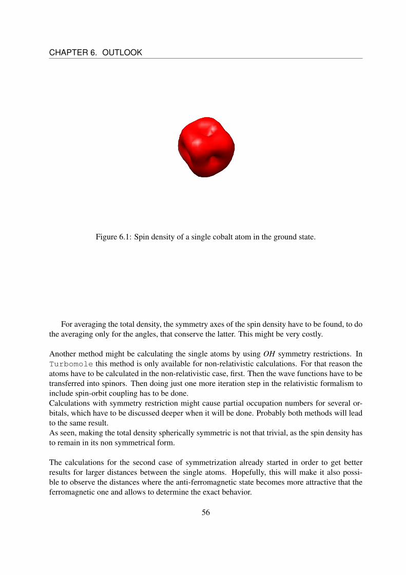
CHAPTER 6. OUTLOOK
Figure 6.1: Spin density of a single cobalt atom in the ground state.
For averaging the total density, the symmetry axes of the spin density have to be found, to dothe averaging only for the angles, that conserve the latter. This might be very costly.
Another method might be calculating the single atoms by using OH symmetry restrictions. InTurbomole this method is only available for non-relativistic calculations. For that reason theatoms have to be calculated in the non-relativistic case, first. Then the wave functions have to betransferred into spinors. Then doing just one more iteration step in the relativistic formalism toinclude spin-orbit coupling has to be done.Calculations with symmetry restriction might cause partial occupation numbers for several or-bitals, which have to be discussed deeper when it will be done. Probably both methods will leadto the same result.As seen, making the total density spherically symmetric is not that trivial, as the spin density hasto remain in its non symmetrical form.
The calculations for the second case of symmetrization already started in order to get betterresults for larger distances between the single atoms. Hopefully, this will make it also possi-ble to observe the distances where the anti-ferromagnetic state becomes more attractive that theferromagnetic one and allows to determine the exact behavior.
56

CHAPTER 6. OUTLOOK
Spin-Dependent Transport Calculations
Figure 6.2: Tunneling junction with gold (Au) leads and Fe, Co or Ni atoms at the very top ofthe tips, to determine the current through this junction.
The implemented rotation tool can be practical for spin dependent transport calculations throughsingle or double atom junctions as it was done in [Burz15]. The expectation value of the fer-romagnetic Fe, Co or Ni atom’s spin in Au−X −Au or Au−X −X −Au junctions (cf. Fig.6.2) with X ∈ Fe, Co, Ni can be controlled and fixed in a defined direction. With it, we candetermine its influence on the transport properties.Indeed, it is needed to expand the formula for the electrical current in the Keldysh formalism (cf.[Cuev10] p. 210). This can be done easily by making the underlying tight-binding Hamiltonianspin-dependent.
Figure 6.3: Sketch of an arbitrary tunneling junction. It includes two leads L, R and a non-specified central part C [Cuev10].
The Hamiltonian for the system in Fig. 6.3 becomes
H = ∑i j,αβ ,σσ ′
hσσ ′
iα, jβ ciασc jβσ ′, (6.1)
where i, j denote the sites, α, β the orbitals and σ , σ ′ the spins. By following the non-equilibrium Greens function formalism in [Cuev10] for the spin-independent current and using
57
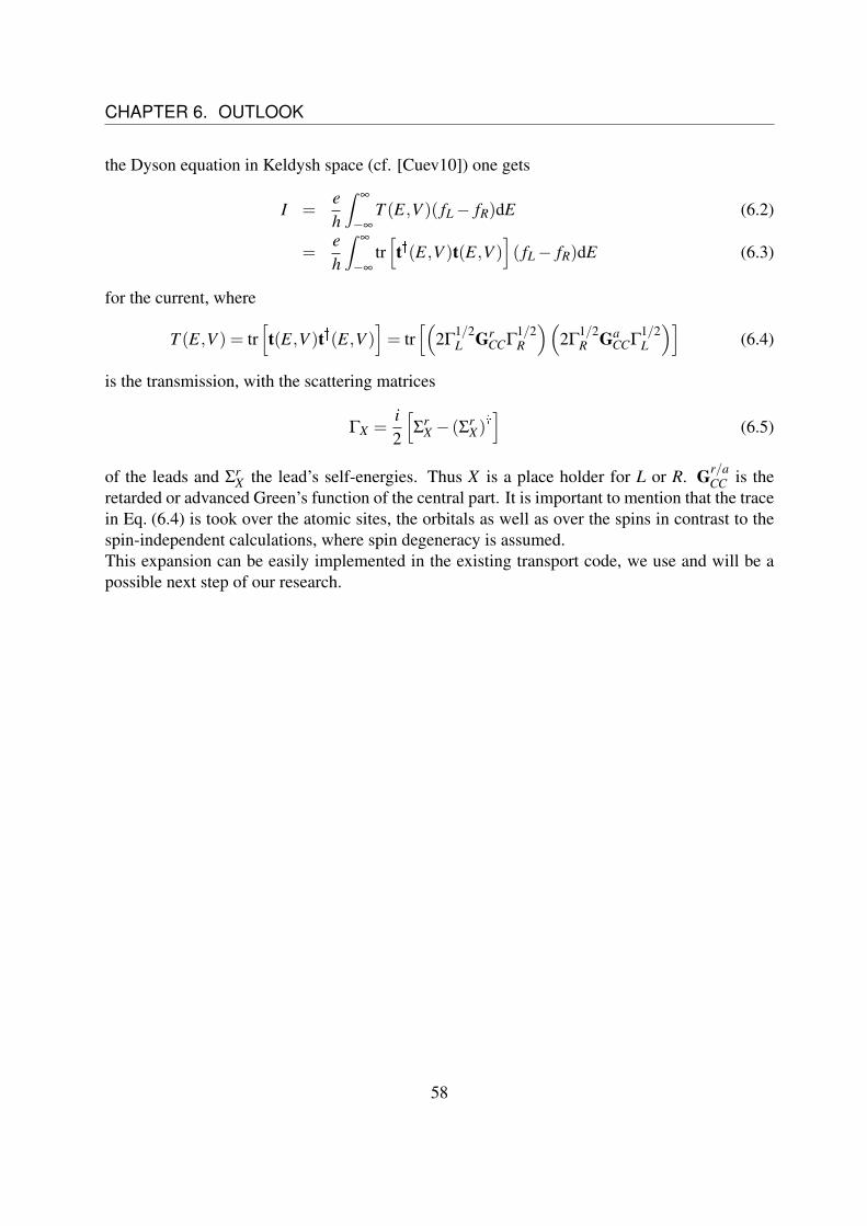
CHAPTER 6. OUTLOOK
the Dyson equation in Keldysh space (cf. [Cuev10]) one gets
I =eh
∫∞
−∞
T (E,V )( fL− fR)dE (6.2)
=eh
∫∞
−∞
tr[t(E,V )t(E,V )
]( fL− fR)dE (6.3)
for the current, where
T (E,V ) = tr[t(E,V )t(E,V )
]= tr
[(2Γ
1/2L Gr
CCΓ1/2R
)(2Γ
1/2R Ga
CCΓ1/2L
)](6.4)
is the transmission, with the scattering matrices
ΓX =i2
[Σ
rX − (Σr
X)]
(6.5)
of the leads and ΣrX the lead’s self-energies. Thus X is a place holder for L or R. Gr/a
CC is theretarded or advanced Green’s function of the central part. It is important to mention that the tracein Eq. (6.4) is took over the atomic sites, the orbitals as well as over the spins in contrast to thespin-independent calculations, where spin degeneracy is assumed.This expansion can be easily implemented in the existing transport code, we use and will be apossible next step of our research.
58

Chapter 7
Conclusion
The spin-lattice couplings of iron and cobalt dimers were analyzed, by studiing the exchangeenergy ∆EXC between two single atomic fragments in a distance interval around the equilibriumdistance d0 for the particular molecule.Therefore, a rotation tool has been implemented adapted to the used Turbomole code, whosealgebra and restrictions were derived.
It was shown that the behavior of the energy ∆EXC depends on the direction of the expecta-tion value of the spin of the single atoms. This behavior is not symmetric and shows a magneticanisotropy.Furthermore, the form of the energy variation was extracted from the calculated energy land-scapes. For both, iron and cobalt, the same characteristics were found. Moreover, the depen-dence on distance of these characteristics was computed.Therewith the Hamiltonian
Hspin =−Dr3
12
(~r12
(~S1 +~S2
))︸ ︷︷ ︸
Huni
− Cr3
12
(~S1~S2−
(~S1~r12
)(~S2~r12
))︸ ︷︷ ︸
Hdip
− Jr4
12
~S1~S2︸ ︷︷ ︸Hsp
(7.1)
was built up to describe the spin-lattice coupling of the system. The Hamiltonian consists of threeterms - one symmetric Heisenberg term Hsp and two terms that induce spin-lattice couplings.
The Dzyaloshinskii-Moriya-like uniaxial spin Hamiltonian Huni shows the characteristic aniso-tropy of single molecular magnets, that is defined by the anisotropy axis of the system. In thestudied case this axis corresponds to the connetion vector~r12 between the two subsystems.The Hamiltonian Hdip describes a magnetic dipolar-dipolar interaction, that is occurring due tospin-lattice coupling. It also induces a magnetic anisotropy and suffices to induce the Einstein-deHaas effect.Finally concrete values for the energy coefficients D, C and J were computed. These values canbe found for iron in Tab. 5.2 and for cobalt in Tab. 5.4, respectively.
59

CHAPTER 7. CONCLUSION
60

Bibliography
[Arm06] M. Armbruster, W. Klopper, F. Weigend, ”Basis-set extensions for two-componentspin-orbit treatments of heavy elements”, Phys. Chem. Chem. Phys, vol. 8, 4862 - 4965,2006
[Arm08] M. Armbruster, F. Weigend, C. van Wullen, W. Klopper, ”Self-consistent treatmentof spin-orbit interactions with efficient Hartree-Fock and density functional theory”, Phys.Chem. Chem. Phys, vol. 10, 1748-1756, 2008
[Ass] M. Assmann, U. Nowak, ”Spin-Lattice Relaxation due to two-side anisotropies”, unpub-lished
[Bar01] S. Baroni, S. de Grioncoli et. al., ”Phonons and related crystal properties from density-functional perturbation theory”, Rev. Mod. Phys. vol. 73, 515 - 526, 2001
[Barn1915] S. J. Barnett, ”Magnetization by rotation”, Phys. Rev. vol. 6, 239, 1915
[Burz15] A. Burtzlaff, A. Weismann, M. Branbyge, R. Berndt, ”Shot Noise as Probe of Spin-Polarized Transport through Single Atoms”, Phys. Rev. Lett. vol 114, 016602, 2015
[Cap02] K. Capelle, ”A Bird’s-Eye View of Density-Functional Theory”, Cond. Mat. Mtrl. Sci.,2006
[Cuev10] J. C. Cuevas, E. Scheer, ”Molecular Electronics - An Introduction to Theory and Ex-periment”, World Scientific, 2010
[Doh75] V. Dohm, P. Fulde, ”Magnetoelastic interaction in rare earth systems”, Z. Phys. B vol.21, 369, 1975
[EdH1915] A. Einstein, W. J. de Haas, ”Experimenteller Nachweis der Ampereschen Moleku-larstrome”, Verh. Dtsch. Phys. Ges. 17, 152, 1915
[Eng02] E. Engel, ”Relativistic Density Functional Theory: Foundations and Basic Formalism”,Theoretical and Computational Chemistry, 2002
[Fed76] P. A. Fedders, R. L. Melcher, ”Rotational pseudospin-phonon interactions at finite fre-quencies”, Phys. Rev. B vol. 14, 1142, 1976
61
BIBLIOGRAPHY
[Fed77] P. A. Fedders, ”Effects of self-consistency on spin-lattice relaxations”, Phys. Rev. B vol.15, 3297, 1977
[Frie96] J. R. Friedmann et. al., ”Macroscopic Measurements of Resonant Magnetization Tun-neling in High-Spin Molecules”, Phys. Rev. Lett. vol 76, 3830, 1996
[Gar15] D. A. Garanin, E. M. Chudnovsky, ”Angular Momentum in spin-phonon processes”,Phys. Rev. B vol. 92, 024421, 2015
[Ham89] M. Hamermesh, ”Group theory and its applications to physical problems”, Dover,1989
[Hon09] J. Honolka et. al., ”Magnetism of FePt Surface Alloys”, Phys. Rev. Lett. vol. 102,067207, 2009
[Ho64] P. Hohenberg, W. Kohn, ”Inhomegeneous Electron Gas”, Phys. Rev. vol. 136, B864-B871, 1964
[Jac12] C.R. Jacob, M. Reihen, ”Spin in Density-Functional Theory”, Int. J. Quantum Chem.vol. 112, 3661-3684, 2012
[Jaaf09] R. Jaafar, E. M. Chudnovsky, D. A. Granin, ”Dynamics of Einstein-de Haas effect:Application to magnetic cantilever”, Phys. Rev. B vol. 79, 104410, 2009
[Ken07] K. G. Dyall, K. Fægri, ”Introduction to RELATIVISTIC QUANTUM CHEMISTRY”,Oxford University Press, 2007
[Ko01] W. Koch, M. C. Holthausen, ”A Chemist’s Guide to Density Functional Theory”, Wiley,2001
[Leh07] J. Lehmann et. al., ”Spin qubits with electrically gated poloxometalate molecules”, Nat.Nano vol. 2, 312 - 317, 2007
[Mas15] A.E. Masunov, S. Gangopadhyay, ”Heisenberg coupling constant predicted for molec-ular magnets with pairwise spin-contamination correction”, J. Mag. Mag. Mat. vol. 369,222 - 227, 2015
[Man09] S. Mankovsky et. al., ”Effects of spin-orbit coupling on the spin structure of depositedtransition-metal clusters”, Phys. Rev. B. vol. 80, 014422, 2009
[Per96] J. P. Perdrew, K. Burke, M. Ernzerhof, ”Generalized gradient approximation made sim-ple”, Rev. Mod. Phys. vol. 77, 3865 - 3868, 1996
[Schwe02] P. Schwerdfeger, ”Relativistic Electronic Structure Theory Part 1. Fundamentals”,Elsevier, 2002
[Su09] P. Su, H. Li, ”Decomposition Analysis of covalent bonds and intermolecular interac-tions”, Chem. Phys. vol. 131, 014102, 2009
62

BIBLIOGRAPHY
[Turb66] Turbomole GmbH, Turbomole Manual 6.6, 2014
[Turb70] Turbomole GmbH, Turbomole Manual 7.0, 2015
[Vle40] J. H. Van Vleck, ”Paramagetic relaxation times for titanium and chrome alum”, Phys.Rev. vol. 57, 426, 1940
[Vle37] J. H. Van Vleck, ”On the anisotropy of Cubic Ferromagnetic Crystals”, Phys. Rev. vol.52, 1178 - 1198, 1937
[Wall06] T. M. Wallis, J. Moreland, P. Kabos, ”Einstein-de Haas effect in a NiFe film depositedon a microcantilever”, Appl. Phys. Lett. vol. 89, 122502, 2006
[Wol02] A. Wolf, M. Reiher, B. A. Hess, ”The generalized Douglas-Kroll transformation” J.Chem. Phys. vol. 117, 9215, 2002
[Zan14] L. Zang, Q. Niu, ”Angular Momentum of phonons and Einstein-de Haas effect”, Phys.Rev. Lett. vol. 112, 085503, 2014
63

BIBLIOGRAPHY
64

Appendix A
Additional calculations
Trigonometric Form of Spin Rotations
In chapter 3.1 the spin rotation u~n (φ) = e−i2~σ ·~n ·φ was transformed in a trigonometric form. In
this chapter the relevant steps are shown. First the exponential function is expanded in a powerseries and sorted by the odd and even summands. It is
e−i2~σ ·~n ·φ =
∞
∑j=0
1j!
[− i
2~σ ·~n ·φ
] j
(A.1)
=∞
∑k=0
(−1)k
2k!
(φ
2
)2k
[~σ ·~n]2k + i∞
∑k=0
(−1)k
(2k+1)!
(φ
2
)2k+1
[~σ ·~n]2k+1 . (A.2)
These sums can be easily simplified by
[~σ ·~n]2 = [nxσx +nyσy +nzσz]2 (A.3)
= n2xσ
2x +nxny (σxσy +σyσx)+nxnz (σxσz +σzσx) (A.4)
+n2yσ
2y +nynz (σyσz +σzσy)+n2
z σ2z (A.5)
= n2xI+nxny (iσz− iσz)+nxnz (−iσy + iσy) (A.6)
+n2yI+nynz (iσx− iσx)+n2
z I (A.7)
=(n2
x +n2y +n2
z)I (A.8)
= I, (A.9)
since~n is a unity vector. Inserting this in Eq. (A.2) we get
u~n (φ) = e−i2~σ ·~n ·φ (A.10)
=∞
∑k=0
(−1)k
2k!
(φ
2
)2k
I+ i∞
∑k=0
(−1)k
(2k+1)!
(φ
2
)2k+1
[~σ ·~n] (A.11)
= Icos(
φ
2
)− i [~σ ·~n]sin
(φ
2
). (A.12)
65

APPENDIX A. ADDITIONAL CALCULATIONS
∆EXC Landscapes of NickelAs mentioned before, the ground state of a nickel dimer is not the high spin state. Thus, theformer calculations might be a bad approximation for that. So the following figures are notanalyzed in detail. The following figures show the same energies and spin states as the figuresshown for iron or cobalt in chapter 5, so they can be threated in the same way. Furthermore, theyshow qualitatively the same behavior as the figures of iron and cobalt.
60180
300 0
60
120
180
-3.2
-3.0
φ1 = φ2 = 0fitfunction
θ1 [deg]
θ2 [deg]
∆EXC [eV]
(a) φ1 = 0, φ2 = 0
-3.2
-3.0
60 180 300
Ene
rgy
∆E
XC
[eV
]
θ1 [deg]
θ2 = 0θ2 = 30θ2 = 60θ2 = 90θ2 = 120θ2 = 150θ2 = 180
(b) φ1 = 0, φ2 = 0
60180
300 0
60
120
180
-2.98
-2.88
θ1 = θ2 = 90fitfunction
φ1 [deg]
φ2 [deg]
∆EXC [eV]
(c) θ1 = 90, θ2 = 90
-2.90
-2.88
60 180 300
Ene
rgy
∆E
XC
[eV
]
φ1 [deg]
φ2 = 0φ2 = 30φ2 = 60φ2 = 90φ2 = 120φ2 = 150φ2 = 180
(d) θ1 = 90, θ2 = 90
Figure A.1: Energy landscape ∆EXC of the Ni dimer dependent on the spin directions of thesubsystem’s spins at equilibrium distance d0 = 3.88 au. (a) Energy dependence on the angles θ1and θ2 of the two spins at φ1 = φ2 = 0, (b) cross sections of the energy landscape in (a), (c)energy dependence on the angles φ1 and φ2 of the two spins at θ1 = θ2 = 90, (d) cross sectionsof the energy landscape in (c). These figures may be used to determine the dependence of theenergy on the spin direction.
66

APPENDIX A. ADDITIONAL CALCULATIONS
-3.2
-3.0
60 180 300
Ene
rgy
∆E
XC
[eV
]
θ1 [deg]
θ2 = 0θ2 = 30θ2 = 60θ2 = 90θ2 = 120θ2 = 150θ2 = 180
(a) φ1 = 0, φ2 = 0
-3.2
-3.0
60 180 300E
nerg
y∆
EX
C[e
V]
θ1 [deg]
θ2 = 0θ2 = 30θ2 = 60θ2 = 90θ2 = 120θ2 = 150θ2 = 180
(b) φ1 = 0, φ2 = 90
-2.90
-2.88
60 180 300
Ene
rgy
∆E
XC
[eV
]
φ1 [deg]
φ2 = 0φ2 = 30φ2 = 60φ2 = 90φ2 = 120φ2 = 150φ2 = 180
(c) θ1 = 90, θ2 = 90
-3.249
-3.247
60 180 300
Ene
rgy
∆E
XC
[eV
]
φ1 [deg]
φ2 = 0φ2 = 30φ2 = 60φ2 = 90φ2 = 120φ2 = 150φ2 = 180
(d) θ1 = 0, θ2 = 0
Figure A.2: Energy landscape ∆EXC of the Ni dimer dependent on the spin directions of thesubsystems’ spins at equilibrium distance d0 = 3.88 au.(a) Energy dependence on the angle θ1for different values of θ2 at φ1 = φ2 = 0, (b) energy dependence for the same situations as(a), but for the angle φ2 = 90, (c) energy dependence on the angle φ1 for different values ofφ2 at θ1 = θ2 = 90, (d) energy dependence for the same situations as (c), but for the anglesθ1 = θ2 = 0. In (d) we expect no dependence on the angle, but there are still some fluctuations.These figures may be used to determine the dependence of the energy on the spin direction.
67
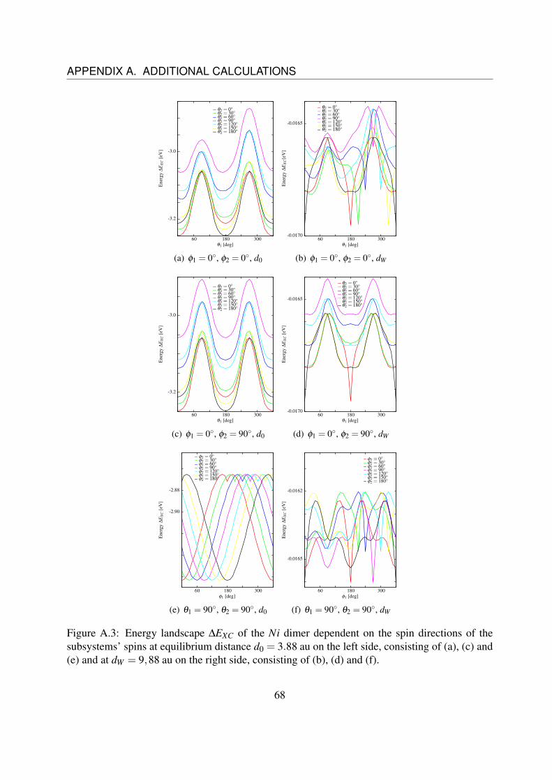
APPENDIX A. ADDITIONAL CALCULATIONS
-3.2
-3.0
60 180 300
Ene
rgy
∆E
XC
[eV
]
θ1 [deg]
θ2 = 0θ2 = 30θ2 = 60θ2 = 90θ2 = 120θ2 = 150θ2 = 180
(a) φ1 = 0, φ2 = 0, d0
-0.0170
-0.0165
60 180 300
Ene
rgy
∆E
XC
[eV
]
θ1 [deg]
θ2 = 0θ2 = 30θ2 = 60θ2 = 90θ2 = 120θ2 = 150θ2 = 180
(b) φ1 = 0, φ2 = 0, dW
-3.2
-3.0
60 180 300
Ene
rgy
∆E
XC
[eV
]
θ1 [deg]
θ2 = 0θ2 = 30θ2 = 60θ2 = 90θ2 = 120θ2 = 150θ2 = 180
(c) φ1 = 0, φ2 = 90, d0
-0.0170
-0.0165
60 180 300
Ene
rgy
∆E
XC
[eV
]
θ1 [deg]
θ2 = 0θ2 = 30θ2 = 60θ2 = 90θ2 = 120θ2 = 150θ2 = 180
(d) φ1 = 0, φ2 = 90, dW
-2.90
-2.88
60 180 300
Ene
rgy
∆E
XC
[eV
]
φ1 [deg]
φ2 = 0φ2 = 30φ2 = 60φ2 = 90φ2 = 120φ2 = 150φ2 = 180
(e) θ1 = 90, θ2 = 90, d0
-0.0165
-0.0162
60 180 300
Ene
rgy
∆E
XC
[eV
]
φ1 [deg]
φ2 = 0φ2 = 30φ2 = 60φ2 = 90φ2 = 120φ2 = 150φ2 = 180
(f) θ1 = 90, θ2 = 90, dW
Figure A.3: Energy landscape ∆EXC of the Ni dimer dependent on the spin directions of thesubsystems’ spins at equilibrium distance d0 = 3.88 au on the left side, consisting of (a), (c) and(e) and at dW = 9,88 au on the right side, consisting of (b), (d) and (f).
68

APPENDIX A. ADDITIONAL CALCULATIONS
-3.249
-3.247
60 180 300
Ene
rgy
∆E
XC
[eV
]
φ1 [deg]
φ2 = 0φ2 = 30φ2 = 60φ2 = 90φ2 = 120φ2 = 150φ2 = 180
(a) θ1 = θ2 = 0, d0
-0.0167
-0.0165
60 180 300E
nerg
y∆
EX
C[e
V]
φ1 [deg]
φ2 = 0φ2 = 30φ2 = 60φ2 = 90φ2 = 120φ2 = 150φ2 = 180
(b) θ1 = θ2 = 0, dW
-3.2
-3.1
60 180 300
Ene
rgy
∆E
XC
[eV
]
φ1 [deg]
θ1 = 0θ1 = 30θ1 = 60θ1 = 90θ1 = 120θ1 = 150θ1 = 180
(c) θ2 = φ2 = 0, d0
-0.0170
-0.0165
60 180 300
Ene
rgy
∆E
XC
[eV
]
φ1 [deg]
θ1 = 0θ1 = 30θ1 = 60θ1 = 90θ1 = 120θ1 = 150θ1 = 180
(d) θ2 = φ2 = 0, dW
Figure A.4: This figure illustrates why the figures on the right side of Fig. 5.10 are unusable for apossible analysis. (a) Variation of energy at the equilibrium distance d0 = 3.88 au dependent onthe angle φ1 for different values of φ2 while θ1 = θ2 = 0 are fixed, (b) the same for dW = 9.88 au,(c) variation of energy at the equilibrium distance d0 dependent on the angle φ1, too, but fordifferent values of θ1 while θ2 = φ2 = 0 are fixed and Fig. (d) the same for dW . These figuresshow a rotation of the spin around the z-axis and thus we expect no angular dependence of theenergy in this case. Nevertheless there are some fluctuations, that contaminate the results.
69

APPENDIX A. ADDITIONAL CALCULATIONS
70
Appendix B
Erklarung
Ich versichere hiermit, dass ich die anliegende Masterarbeit mit dem Thema
Microscopic Studies of Spin-Lattice Couplings
selbstandig verfasst und keine anderen Hilfsmittel und Quellen als die angegebenen benutzt habe.
Die Stellen, die anderen Werken (einschließlich des Internets und anderer elektronischer Text-und Dateisammlungen) dem Wortlaut oder dem Sinn nach entnommen sind, habe ich in jedemeinzelen Fall durch Angabe der Quelle bzw. der Sekundarliteratur als Entlehnung kenntlichgemacht.
Weiterhin versichere ich hiermit, dass die o.g. Arbeit noch nicht anderweitig als Abschlussarbeiteiner Diplom-, Bachelor bzw. Masterprufung eingereicht wurde. Mir ist ferner bekannt, dass ichbis zum Abschluss des Prufungsverfahrens die Materialien verfugbar zu halten habe, welche dieeigenstandige Abfassung der Arbeit belegen konnen.
Die Arbeit wird nach Abschluss des Prufungsverfahrens der Bibliothek der Universitat Konstanzubergeben und katalogisiert. Damit ist sie durch Einsicht und Ausleihe offentlich zuganglich.Die erfassten beschriebenen Daten wie z.B. Autor, Titel usw. stehen offentlich zur Verfugungund konnen durch Dritte (z.B. Suchmaschinenbetreiber oder Datenbankbetreiber) weiterverwen-det werden.Als Urheber der anliegenden Arbeit stimme ich diesem Verfahren nicht zu.
Ort, Datum Unterschrift
71