Microfluidics for Fuel Cell Applications

by

Ian Stewart

BASc, University of Toronto, 2008

A Thesis Submitted in Partial Fulfillment

of the Requirements for the Degree of

MASTER OF APPLIED SCIENCE

in the Department of Mechanical Engineering

© Ian Stewart 2011

University of Victoria

All rights reserved. This thesis may not be reproduced in whole or in part, by photocopy

or other means, without the permission of the author.

ii

Supervisory Committee

Microfluidics for Fuel Cell Applications

by

Ian Stewart

BASc, University of Toronto, 2008

Supervisory Committee

Dr. David Sinton (Department of Mechanical Engineering)

Co-Supervisor

Dr. Ned Djilali (Department of Mechanical Engineering)

Co-Supervisor

Dr. David Harrington (Department of Chemistry)

Outside Member

iii

Abstract

Supervisory Committee

Dr. David Sinton (Department of Mechanical Engineering) Co-Supervisor

Dr. Ned Djilali (Department of Mechanical Engineering) Co-Supervisor

Dr. David Harrington (Department of Chemistry) Outside Member

In this work, a microfluidics approach is applied to two fuel cell related projects; the study of

deformation and contact angle hysteresis on water invasion in porous media and the introduction of

bubble fuel cells. This work was carried out as collaboration between the microfluidics and CFCE groups

in the Department of Mechanical Engineering at the University of Victoria.

Understanding water transport in the porous media of Polymer Electrolyte Membrane fuel cells is

crucial to improve performance. One popular technique for both numeric simulations and experimental

micromodels is pore network modeling, which predicts flow behavior as a function of capillary number

and relative viscosity. An open question is the validity of pore network modeling for the small highly

non-wetting pores in fuel cell porous media. In particular, current pore network models do not account

for deformable media or contact angle hysteresis. We developed and tested a deformable microfluidic

network with an average hydraulic diameter of 5 μm, the smallest sizes to date. At a capillary number

and relative viscosity for which conventional theory would predict strong capillary fingering behavior,

we report almost complete saturation. This work represents the first experimental pore network model

to demonstrate the combined effects of material deformation and contact angle hysteresis.

Microfluidic fuel cells are small scale energy conversion devices that take advantage of microscale

transport phenomena to reduce size, complexity and cost. They are particularly attractive for portable

electronic devices, due to their potentially high energy density. The current state of the art microfluidic

fuel cell uses the laminar flow of liquid fuel and oxidant as a membrane. Their performance is plagued

by a number of factors including mixing, concentration polarization, ohmic polarization and low fuel

utilization. In this work, a new type of microfluidic fuel cell is conceptualized and developed that uses

bubbles to transport fuel and oxidant within an electrolyte. Bubbles offer a phase boundary to prevent

iv

mixing, higher rates of diffusion, and independent electrolyte selection. One particular bubble fuel cell

design produces alternating current. This work presents, to our knowledge, the first microfluidic chip to

produce bubbles of alternating composition in a single channel, class of fuel cells that use bubbles to

transport fuel and oxidant and fuel cell capable of generating alternating current.

v

Table of Contents

Supervisory Committee ................................................................................................................................ ii

Abstract ........................................................................................................................................................ iii

Table of Contents .......................................................................................................................................... v

List of Figures .............................................................................................................................................. vii

Nomenclature ............................................................................................................................................... x

Acknowledgements ..................................................................................................................................... xii

1 Introduction .......................................................................................................................................... 1

1.1 Motivation ..................................................................................................................................... 1

1.2 Fuel Cell Principles ........................................................................................................................ 2

1.3 Thermodynamics of Fuel Cells ...................................................................................................... 3

1.4 Operation and Losses of Fuel Cells ............................................................................................... 5

1.5 Microscale Transport Phenomena ................................................................................................ 7

1.6 Multiphase Flow in Microfluidics .................................................................................................. 9

1.7 Gas Diffusion Layer of PEM Fuel Cells ......................................................................................... 10

1.8 Microfluidic Fuel Cells ................................................................................................................. 10

1.9 Thesis Overview and Contributions ............................................................................................ 11

2 Experimental Methods........................................................................................................................ 13

2.1 Microfluidic Fabrication Background .......................................................................................... 13

2.2 Photolithography ........................................................................................................................ 13

2.3 PDMS ........................................................................................................................................... 14

2.4 Fluorescent Imaging .................................................................................................................... 15

3 Liquid Transport in PEMFCs and Pore Network Modeling .................................................................. 16

3.1 PEMFC Water Management ....................................................................................................... 16

3.2 Key Terms for Analysis of Liquid Transport in Porous Media ..................................................... 17

3.3 Modeling Techniques and Pore Network Models ...................................................................... 18

4 Deformability and Hysteresis in Pore Network Models...................................................................... 23

4.1 Introduction ................................................................................................................................ 23

4.2 Experimental Preparation ........................................................................................................... 23

4.3 Results and Discussion ................................................................................................................ 25

vi

4.3.1 Effects of Deformation on Network Morphology ............................................................... 25

4.3.2 Effects of Contact Angle Hysteresis on Network Saturation .............................................. 29

4.3.3 Modifications to the Invasion Percolation Algorithm ......................................................... 33

4.4 Summary ..................................................................................................................................... 35

5 A Micro Bubble Fuel Cell (ACDCμFC) .................................................................................................. 36

5.1 Introduction ................................................................................................................................ 36

5.2 Classification of Microfluidic Bubble Fuel Cells........................................................................... 39

5.3 Experimental Preparation ........................................................................................................... 42

5.4 Results and Discussion ................................................................................................................ 43

5.4.1 Type 1 .................................................................................................................................. 43

5.4.2 Type 2 .................................................................................................................................. 44

5.5 Summary ..................................................................................................................................... 48

6 Conclusions and Future Work ............................................................................................................. 49

6.1 Future Pore Network Modeling Work ........................................................................................ 49

6.1.1 A PDMS Pore Network Model with Limited Entry Points ................................................... 49

6.2 Future microfluidic fuel cells ....................................................................................................... 50

6.2.1 Future work in Microfluidic Bubble Fuel Cells .................................................................... 50

6.3 Microfluidic bubble combustion ................................................................................................. 51

7 Bibliography ........................................................................................................................................ 54

8 Appendix A Mathematica Code for Pore Network Generation .......................................................... 63

vii

List of Figures

Figure 1-1 Fuel Cell schematic. Fuel and Oxidant are continuously supplied to the electrodes.

Electrochemical reactions occur on the anode and cathode. The high electrical resistance

and ionic conductivity of the electrolyte allow ions to cross from anode to cathode, but

electrons must go through an external circuit, doing work to complete the chemical

reaction................................................................................................................................ 2

Figure 1-2 A fuel cell polarization curve. Deviations from the ideal open circuit value are caused by

(in order of increasing current) activation polarization, ohmic polarization and

concentration polarization. Integration of this polarization curve would give power

density, which peaks in the concentration polarization regime. ......................................... 5

Figure 1-3 Capillary pressures illustrated with a simple diagram showing a hydrophobic, b neutral

and c hydrophilic tubes placed in a beaker of water. .......................................................... 8

Figure 1-4 A microfluidic bubble train that controls colloidal quantum dot assembly. A fluorescent

tracer was used to highlight the aqueous phase. Scale bar represents 500µm. (Image

courtesy of CW Wang, University of Victoria) .................................................................. 9

Figure 2-1 Fluorescence microscope. Key components include the light source, excitation filter,

dichoric mirror, objective and the emission filter. ............................................................ 15

Figure 3-1 Schematic Log Log map describing fluid flow in porous media as a function of relative

viscosity (M) and capillary number (Ca). This pore network map assumes no contact

angle hysteresis or material deformation .......................................................................... 19

Figure 4-1 Schematic of Experimental Set up. 1st blowout shows a 4x4 randomly distributed

network. The 2nd blowout shows an SEM image of the SU-8 master at high

magnification. ................................................................................................................... 24

Figure 4-2 Fluorescent dye images in 5 μm hydrophobic channels incased in 5 mm of PDMS. a

Water saturated 5μm x 50μm lead channel shows a hemispherical cap and frontal

deformation. Red lines show boundaries to inlet manifold. b Water enters the inlet

manifold, leading to a reduction in pressure and material deformation. The time between

a and b was 5 seconds. c Water saturated network begins breakthrough process continued

at 15 second intervals in d and e. f Shows subtraction of highlighted red regions d from c

and e from d to demonstrate deformation effects. Image a and image b are raw images, c-

f are converted to black and white, inverted, and contrast enhanced. ............................... 25

Figure 4-3 Stress-Strain data from Sadeghi (2011) with a fit for points below a strain of 0.1 to

approximate the linearized region. .................................................................................... 28

Figure 4-4 Images showing the effect of hysteresis on the contact angle of water invading the PDMS

network. Dotted line indicates the approximate contact point between the liquid and the

viii

walls. a Liquid water was introduced into a 10 µm x 10 µm channel. The contact angle

can be seen to be approximately 105°, as the meniscus is in front of the wetted perimeter.

b When flow is reversed the liquid water meniscus retreats, corresponding to a contact

angle around 85° ............................................................................................................... 29

Figure 4-5 Microscopy images showing invasion into a hydrophobic network at a capillary number

of 10-6. a Invasion begins at a single node that branch into the network. b Saturation

proceeds toward the bulk network bulk and outlet. c Large scale localized saturation can

be seen as breakthrough occurs. d Breakthrough and saturation along the outlet manifold

leads to saturation back into the network. All images converted to black and white,

inverted, and contrast enhanced. ....................................................................................... 30

Figure 4-6 Fluorescent dye images of a hydrophobic network invaded at flow rates corresponding to

a capillary number of 10-10. In a invasion occurs along a single row of nodes toward the

outlet. In b the invasion then branches in the two lateral directions and two separate

invasion points enter the network. c Invasion points consolidate and multiple trapping

events can be identified. d Breakthrough occurs. Trapping events seen in c have

disappeared and new ones have formed. Time between images was, in order, 12 minutes

30 seconds, 21 minutes 30 seconds and 46 minutes 50 seconds. Images were converted to

black and white and contrast enhanced. ............................................................................ 32

Figure 4-7 Schematic explanation of different wetting patterns expected and observed in the

microfluidic network. a Original invasion percolation behavior with no deformation and

no contact angle hysteresis. Narrow saturated nodes recede during pressure drops and

saturation at breakthrough is approximately 50%. b Invasion with deformation and

contact angle hysteresis. Deformation occurs in the first image leading to an increase in

hydraulic radii of the saturated pores and subsequent invasion. No receding from small

pores occurs due to contact angle hysteresis. In the third image breakthrough occurs and

back filling leads to a final saturation of over 90%. ......................................................... 34

Figure 5-1 Schematic of a laminar flow fuel cell. Liquid fuel and oxidant are pumped separately

from the top. Due to the low Reynolds number, the fluid behavior is laminar and mixing

is diffusion limited. Electrodes are placed at the side to draw current, and ions travel

across the two liquids in the horizontal direction. Mass transport effects cause depletion

regions to form at the anode and cathode, and non-reversible mixing occurs at the fuel

and oxidant boundary. ....................................................................................................... 37

Figure 5-2 Schematic and image of a Type 1 micro bubble fuel cell. In a T1 shows the initial system,

which is a single channel with gold electrodes on the bottom. At T2 a battery is used to

electrolyze the electrolyte, producing hydrogen and oxygen. At T3 fluid flow through the

system moves the bubbles down the channel, and current can be drawn. b is an image of

the actual device. The entire microbubble fuel cell fits on a 25mm x 75 mm glass slide. 40

Figure 5-3 Schematic of a single channel fuel cell that generates alternating current. a Details of the

electrochemical Hydrogen Oxidant Reaction (HOR) and Oxygen Reduction Reaction

(ORR) and the transfer of ions through solution and electrons through an external circuit.

ix

b Movement of H2 and O2 bubbles under an external force: Over time bubbles move from

one electrode to the next (1-3), reversing current direction. c Voltages generated by the

device under operation. ..................................................................................................... 41

Figure 5-4 Schematic of a Type 3 micro bubble fuel cell. a gives a top view of the system. Gas

slugs enter into the channels through T junctions. Fuel and oxidant travel down

independent channels over electrodes. A PDMS barrier provides a separator. b clarifies

the setup with a down the line view, showing the bubbles in the channel, electrodes on

the bottom and separator. .................................................................................................. 42

Figure 5-5 Images taken at closed circuit to infer current in a Type 1 bubble fuel cell. Image b was

taken 80 seconds after Image a. The flow rate is 0, electrolyte 1M KOH. Analysis of the

decrease in bubble size corresponded to a current of 1 μAmp. ........................................ 44

Figure 5-6 Sequential images of alternating bubble creation in a double-T junction. a Stream of air

from right gas reservoir enters the main channel. b Invading fluid squeezes off entire

channel, a small liquid barrier prevents mixing with opposite gas channel. c-d Liquid

fluid, blocked off from the main downstream channel, enters the opposing gas channel,

increasing buffer width. e Gas segment separates from right gas reservoir and moves

downstream. f Pressure from liquid entering the left gas channel stops, air from left gas

reservoir enters main channel. Blowouts added for detail. ............................................... 45

Figure 5-7 a Autocad design for the “bowtie” T channels and mask for the gold electrode layer. The

mold from the top mask fits directly on top of the gold electrode. The dimensions of both

of these chips are 25mm x 75mm. The switchback area is where bubbles of alternating

composition will produce an AC voltage. b Image of a test system (narrowing neck) with

no electrodes. Used to test capability of generating alternate slugs .................................. 46

Figure 5-8 Test chip demonstrating consistent gas/liquid slug sizes. Flow rates were 25 μl/min for

the liquid and 15 μl/min for each gas. ............................................................................... 47

Figure 6-1 Schematic and image of microbubble combustion. In a, dual T junctions are used to

produce alternating bubbles of fuel and oxidant in a single channel. At b microfluidic

pillars trap the first bubble and remove the liquid between, causing the fuel and oxidant to

merge. At c the combustible bubble travels over two thinly spaced metal leads, where a

high voltage pulse produces combustion. ......................................................................... 52

x

Nomenclature

Symbol Description

α Charge transfer coefficient

A Area

Ca Capillary number

E Electric potential

Eeq Equilibrium potential

F Faradays constant

G Gibbs free energy

g Shear modulus

H Enthalpy

iL Limiting current

io Exchange current density

k Permeability

λ Rubber extension ratio

L Characteristic length

M Relative viscosity

n Number of moles

η Efficiency

ηconc Concentration overpotential

Pc Capillary pressure

Partial pressure

ρ Density

r Radius

Ω Resistance

xi

R Universal gas constant, 8.314 J K-1 mol-1

S Entropy

T Temperature

μ Dynamic viscosity

μi Invading fluid viscosity

μd Displaced fluid viscosity

V Velocity

ϒ Surface tension

xii

Acknowledgements

I would first like to thank Dr. Sinton and Dr. Djilali for meeting with me in the summer of 2008, taking

me on as a co-supervised student the following fall and for giving guidance throughout my masters. I

especially owe them gratitude in providing me an interesting and challenging project for the first half of

my thesis and the freedom to pursue something entirely unrelated in the latter half.

The microfluidics group has provided me great feedback on everything microfluidics throughout my two

years at the University of Victoria. In particular I would like to thank Brent Scarff, Carlos Escobedo, Slava

Berejnov, the carbon (burn and bury) group and the biofuels group for all of their advice. The CFCE

group has balanced that by providing their extensive knowledge on everything fuel cells.

Finally I’d like to thank my parents and two sisters for their support in everything I do, my girlfriend

Kristin for giving me happiness and balance, and our dog Honey for walks every morning.

1 Introduction

1.1 Motivation In 2008 the world’s energy consumption was 1.32×1014 kWh (IEA 2010). Of this, over 89% was produced

through the combustion of fossil fuels, and 27% was for point of use in the transportation industry. The

extraction and burning of coal, oil and natural gas contribute to a variety of adverse effects to the globe

including but not limited to a proliferation of greenhouse gases, decrease in air quality and a rise in sea

levels and ocean acidity (Brown 08). In the long term, this trend is unsustainable; the resources of coal,

natural gas and oil are finite, and nature’s current production is orders of magnitude less than current

consumption. In order to change the current energy system to be environmentally sustainable, two

major shifts are suggested (Scott 2008). First is a shift of energy sources from coal, natural gas and oil

toward renewable or non-carbon emission sources such as sunlight, wind, tidal, biomass growth or

nuclear power. The second shift is in energy currencies that are consumed at point of use from gasoline

based fuels to a non-carbon emitting currency, such as hydrogen.

Fuel cells are electrochemical devices that convert chemical energy to electricity and are

thermodynamically more efficient than combustion engines (Li 2007). Fuel cells have been developed to

use a very wide range of fuels, including those that emit carbon dioxide, although most current research

focuses on the use of hydrogen and oxygen. While fuel cell research is promising, and has the great

potential of changing the way the world converts energy, there are quite a few barriers preventing

widespread adoption. The principal issue is cost, as automotive fuel cells are currently 10-100x more

expensive than internal combustion engines (US DOE 2004). These costs include the production of

hydrogen and its storage, fuel cell components and a distribution infrastructure. While many different

types of fuel cells have been developed, the most promising for automotive applications are polymer

electrolyte membrane fuel cells (PEMFC). For small scale devices, consumer demand for increased

energy capacity in portable electronic devices has led to research in fuel cells, which can offer

considerably higher energy densities then batteries (Dyer 2002). A novel branch of these miniaturized

electrochemical devices, microfluidic fuel cells, use unconventional designs that exploit microscale

transport phenomena.

This chapter begins with an introduction to fuel cells covering basic thermodynamic and electrochemical

principles. The next section gives a brief overview of microfluidics followed by its application to the two

fuel cell projects that are the core of this thesis; studying the effects of deformation and hysteresis in a

2

microfluidic pore network (a technique employed to understand transport processes in PEMFCs) and the

design of a fuel cell that use bubbles to transport fuel and oxidant.

1.2 Fuel Cell Principles Fuel cells differentiate themselves from other electrochemical cells by having an external supply of fuel,

in contrast to batteries which store their fuel internally. A basic schematic of a fuel cell is shown in

Figure 1-1. A fuel cell consists of 4 main components; fuel, oxidant, an electrolyte and electrodes. The

fuel and oxidant provide chemical potential. The electrodes (anode and cathode) serve as a catalyst for

the chemical reaction, and provide contacts for electron transfer. Finally the electrolyte is conductive to

ions and has a high electronic resistance. This allows ions to cross freely between the anode and

cathode. In order to complete the chemical reaction, electrons travel along an external circuit, where

work can be drawn. The ion conductor is typically a solid membrane or an encased liquid.

Figure 1-1 Fuel Cell schematic. Fuel and Oxidant are continuously supplied to the electrodes. Electrochemical

reactions occur on the anode and cathode. The high electrical resistance and ionic conductivity of the

electrolyte allow ions to cross from anode to cathode, but electrons must go through an external circuit,

doing work to complete the chemical reaction.

For a typical fuel cell, hydrogen and oxygen are entered into the system; hydrogen from a storage tank

of either liquefied or compressed hydrogen, oxygen from ambient air or a storage tank. For a Polymer

3

Electrolyte Membrane Fuel Cell (PEMFC) or Phosphoric Acid Fuel Cell (PAFC) hydrogen is exposed to the

anode catalyst, which is made of platinum, and is oxidized in the reaction

(1.2.1)

The electrons from the reaction are conducted along the electrode assembly through a circuit. The

hydrogen ions diffuse through the polymer electrolyte membrane to the cathode. In the presence of

hydrogen ions, two electrons, and the cathode, the oxygen reacts to form water

(1.2.2)

Leading to an overall cell reaction of

(1.2.3)

Hydrogen fuel cells differentiate from each other by their electrolyte material, charge carrier and

operating conditions. A more detailed explanation of anodic and cathodic reactions, advantages and

disadvantages of particular fuel cell types can be found in fuel cell textbooks (Mench 2008) or publically

available handbooks (US DOE 2004).

1.3 Thermodynamics of Fuel Cells This section presents the general thermodynamic and electrochemical relations describing fuel cell

performance. More in depth derivations and discussion are available in the aforementioned texts on

fuel cells and can also be found in texts on electrochemistry (Bard 2001) and thermodynamics

(Struchtrup 2009).

The total possible reversible work available at constant temperature and pressure for a chemical

reaction is given by the Gibb’s free energy, ΔG. Considering a standard cell reaction, like those in the

preceding section represented as

(1.3.1)

The change in Gibbs free energy of a process can be written as the difference between the Gibbs free

energy of formation for the products subtracted by the Gibbs free energy of formation for the reactants

(1.3.2)

The Gibbs free energy is a state function. Two useful electrochemical relationships assist in identifying

its value, first

4

(1.3.3)

where H ,the enthalpy, and S the entropy can be measured as a function of temperature, given suitable

reference values. There also exists a relationship between the Gibbs free energy and electrical potential

of a process

(1.3.4)

Where n is the number of moles, F is Faraday’s constant or the number of coulombs per mole, and E is

electrical potential, in volts. The change in for a reaction can be found via the Nernst equation, which

shows the Gibbs free energy as a function of its value at standard state, , temperature and the

partial pressures of reactants and products.

(1.3.5)

In terms of potential, the Nernst equation can be rewritten in terms of voltages as

(1.3.6)

is in the standard potential of the reaction at 298 K. For the hydrogen-oxygen reaction the

equilibrium voltage is 1.23 volts (for water product) and 1.18 volts for gaseous products.

With the Nernst equation and a way to measure the Gibb’s free energy, it is possible to calculate the

ideal efficiency of a fuel cell. The thermal efficiency of a fuel cell is defined as the useful energy

produced by a system divided by the enthalpy,

(1.3.7)

At standard conditions, this gives a maximum thermal efficiency of hydrogen fuel cells of at

25° C. Currently the world uses combustion engines almost exclusively for automotive and electric

power generation. Combustion engines work by burning fuel, creating heat. The conversion of heat into

useable energy was studied by Carnot. Carnot found that the efficiency of a heat engine is theoretically

limited to a maximum of

, where Tc is the temperature of the cold reservoir and Th is the

temperature of the hot reservoir. For automotives, which at best have Tc at ambient temperature, ideal

efficiencies are limited to around 45%. The ideal thermodynamic efficiency is based around the

maximum reversible work available, which implies an infinitesimally slow process. In real world uses,

5

both fuel cells and internal combustion engines are employed to provide high power and actual

efficiencies are more dependent on materials used and actual system design.

1.4 Operation and Losses of Fuel Cells For a given power output, fuel cells are too expensive to compete commercially with current internal

combustion engines. In order to decrease costs, present fuel cell research is focused on either

decreasing costs of components or increasing power density. By increasing the power density, fuel cells

can be smaller, and decrease the materials used. Operating at maximum power density introduces

losses from a variety of sources and for optimal power output each must be addressed to some degree.

The amount of power derived from a fuel cell is dependent on its operating current. Inefficiencies in a

fuel cell as a function of current can be seen in a Current versus Potential graph, Figure 1-2. At zero

current, the open circuit voltage of the fuel cell is slightly less than that of the theoretical equilibrium

voltage. At low currents, losses are principally due to activation polarization, at medium currents ohmic

polarization and at high current density concentration polarization. Current state of the art PEM Fuel

cells reach peak power density in the domain between ohmic losses and mass transport effects.

Therefore, all of the described losses contribute to limiting fuel cell performance and must be addressed

in order to improve fuel cell power density.

Figure 1-2 A fuel cell polarization curve. Deviations from the ideal open circuit value are caused by (in order of

increasing current) activation polarization, ohmic polarization and concentration polarization.

6

Activation losses are caused by inefficient electrode kinetics. Losses on a single electrode can be

represented by the Bulter-Volmer equation for (E-Eeq), the activation over potential.

(1.4.1)

Where I is the current, io is the exchange current density, E is the electrode potential, Eeq is the

equilibrium potential, A is the active surface area, T is the temperature in K, n is the number of charge

carriers, F is faradays constant, R is the universal gas constant and α is the charge transfer coefficient.

The loss due to activation potential is dependent on the activity of the catalysts, the charge transfer

reactions and the temperature at which the system is operating. Chemical reactions on both the anode

and cathode, contribute to the losses in activation overpotential.

Ohmic losses are caused by the resistance of charge moving within the cell. A fuel cell can be

represented as a complete circuit, where electrons are charge carriers through the electrodes and ions

through the electrolyte. These individual resistances contribute in series to produce a cumulative cell

resistance. In Figure 1-2, the middle portion of the curve has a linear relationship between the current

and voltage, where the slope is the cells resistance, in accordance to Ohm’s Law. Electric resistances are

dependent on the materials and their geometry. Ionic resistance is dependent on the mobility of the

charge carrier, the membrane geometry and conductivity.

Concentration polarization is caused by mass transport limitations. In a fuel cell, reactions occur at the

catalyst, which are part of the electrode assembly. If these reactions occur at too high of a rate reactants

will be depleted in the electrode vicinity. This forms a concentration gradient of reactants and is limited

by diffusion. The magnitude of this loss can be given by concentration polarization, which is derived

from Fick’s law

(1.4.2)

Where R is the gas constant, T is the temperature in Kelvin, z is the charge per ion, F is Faradays

constant, i is the operating current, and iL is the limiting current. When i << iL, this effect is negligible,

however it increases exponentially at higher currents.

7

1.5 Microscale Transport Phenomena Microfluidics considers fluids confined by at least one length scale between 1-300 micrometers or fluid

volumes of 10-18 – 10-9 liters. Microfluidics was originally started in the field of analysis, where a wide

variety of advantages including low cost, small required samples and reagent amounts and high

sensitivity led to a large initial growth in interest (Whitesides 2006). The introduction of Polydimethyl-

siloxane (PDMS) as an inexpensive, tunable, biocompatible and optically transparent soft elastomer

allowed a wide variety of fields to apply microfluidic techniques. With attributes such as direct visual

observation through transparent materials, the ability to create feature sizes ranging over 3 orders of

magnitude, fast fabrication and low cost, microfluidics is an excellent technique for designing and

building experiments. Chapter 2 gives an overview of experimental methods used to fabricate

microfluidic devices.

Of particular interest in microfluidics and to this thesis is the effect of decreasing length scales. Chapters

3 and 4 concern is how small scale effects change wetting patterns in porous media. Chapter 5 applies

microscale phenomena to design a new type of fuel cell. Non-dimensional numbers can provide context

to the dominant forces for fluids in microchannels how they differ from macroscale behavior.

The Reynolds number describes the ratio between inertial forces and viscous forces. It is represented as

(1.5.1)

where ρ is the density, V is the velocity, L is the characteristic length scale and µ is the viscosity of the

fluid. For water in a channel of 1- 100 µm and at velocities of 1 µm/s – 1 cm/s, the Reynolds number is

generally on the order of 10-6 – 10 (Squires and Quake 2005). The transition between laminar flow,

where liquids flow parallel to each other and do not readily mix, and turbulent flow occurs at a Reynolds

number of 103. For this reason, most microfluidic networks exhibit laminar flow, and the only mode of

mixing in parallel flowing fluids is diffusion.

The capillary number compares the magnitude of viscous forces to surface tension between immiscible

phases. The dimensionless number Ca is represented as

(1.5.2)

8

Where µ and V have the same definitions for Re, and γ is the surface tension. In large regions and at high

velocities viscous forces will dictate flow behavior, however in viscous fluids or at low flow rates surface

tension and the interactions between phases (gas, liquid and solid) dominate.

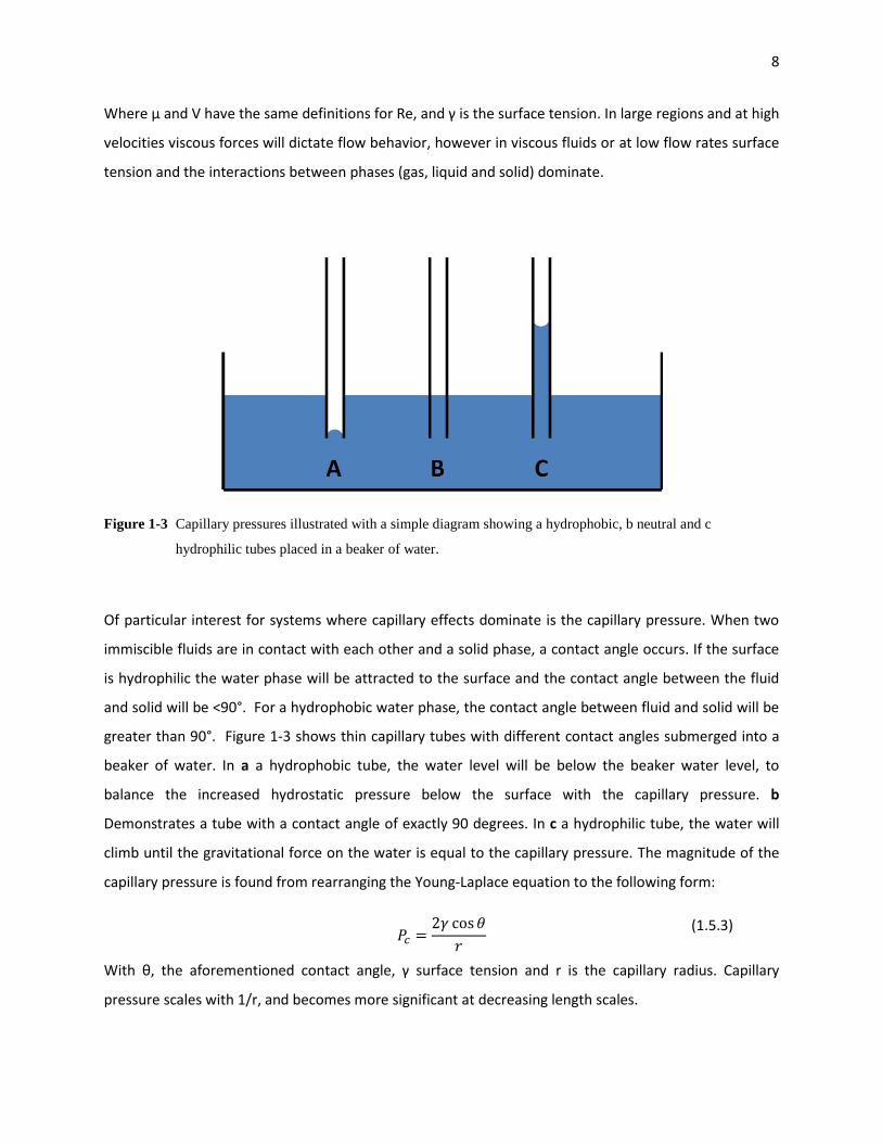
Figure 1-3 Capillary pressures illustrated with a simple diagram showing a hydrophobic, b neutral and c

hydrophilic tubes placed in a beaker of water.

Of particular interest for systems where capillary effects dominate is the capillary pressure. When two

immiscible fluids are in contact with each other and a solid phase, a contact angle occurs. If the surface

is hydrophilic the water phase will be attracted to the surface and the contact angle between the fluid

and solid will be <90°. For a hydrophobic water phase, the contact angle between fluid and solid will be

greater than 90°. Figure 1-3 shows thin capillary tubes with different contact angles submerged into a

beaker of water. In a a hydrophobic tube, the water level will be below the beaker water level, to

balance the increased hydrostatic pressure below the surface with the capillary pressure. b

Demonstrates a tube with a contact angle of exactly 90 degrees. In c a hydrophilic tube, the water will

climb until the gravitational force on the water is equal to the capillary pressure. The magnitude of the

capillary pressure is found from rearranging the Young-Laplace equation to the following form:

(1.5.3)

With θ, the aforementioned contact angle, γ surface tension and r is the capillary radius. Capillary

pressure scales with 1/r, and becomes more significant at decreasing length scales.

9

1.6 Multiphase Flow in Microfluidics Capillary forces and phase boundaries have also been used extensively in two phase microfluidic

reactors. Recently Gunther and Jensen (2006) thoroughly reviewed multiphase flow characteristics in

microchannels. Under certain conditions, reactants will travel down microscale channels in plugs or

bubble/droplet trains. Song et al (2003) demonstrated that independent droplets moving down a

channel experience dipolar flow, which induces chaotic advection. The compartmentalization of phases

results in greatly increased mixing and reduced dispersion (Squires and Quake 2005). Figure 1-4 shows

the application of a droplet train to assist in chemical synthesis by promoting mixing. In research

conducted at the University of Victoria (Schabas 2008a; Schabas 2008b; Wang 2009) colloidal quantum

dots were synthesized in a microfluidic channel.

Figure 1-4 A microfluidic bubble train that controls colloidal quantum dot assembly. A fluorescent tracer was used

to highlight the aqueous phase. Scale bar represents 500µm. (Image courtesy of CW Wang, University

of Victoria)

Recently, additional applications of multiphase flow have been developed. Zheng (2004) demonstrated

the ability to create alternating droplets down a single channel. Hung (2005) advanced this technique

using an architecture that resembled a bowtie to produce and merge alternating droplets in ratios of

1:1, 1:2 and 3:1. Niu et al (2008) created a microfluidic chip that induces consecutive droplets in a

channel to merge.

Two intriguing works have applied the discrete properties of bubbles in microfluidic systems. Prakash

and Gershenfeld (2007) created an all fluid system that uses bubbles as logic bits and capable of

universal computation. In this work, the presence of a bubble influenced flow behavior in the network

to produce Boolean expressions. Hashimoto (2009) similarly used the difference of optical properties

between droplets and a stained liquid to create bits for encoding messages.

10

1.7 Gas Diffusion Layer of PEM Fuel Cells Of all the different types of fuel cells, PEMFCs are the front runner in terms of current performance and

proximity to market penetration in automotive applications. For this reason current research funding for

PEMFCs is currently greater than all other fuel cell types combined (Mench 2008). The advantage of the

PEMFC over alternatives is its polymer membrane, which offers high ionic conductivity at a low

temperature, as well as fast response times to varying load demands and important cost and safety

reductions involving handling, manufacturing and sealing. However, the sub 100°C temperatures lead to

the formation of liquid water at catalyst sites, with the detrimental effect of increasing concentration

polarization losses.

Current PEM fuel cells place a thin <400 µm porous transport layer (PTL) between the fuel and oxidant

flow plates and electrodes. The main function of the PTL is to allow gas diffusion to the catalyst sites and

facilitate liquid water removal. Of particular interest in PEMFCs research is extending the transition

between ohmic losses and mass transport effects to improve power density. However there are

difficulties in measuring water transport in PEM fuel cells due to the randomized pore structure of the

media, opaque materials and small length scales. This has made understanding the mechanisms and

improving the PTL subject of significant fuel cell research (Bazylak 2007; Costamanga and Srinivasan

2001; Mukherjee 2011). One technique for modeling liquid transport in the PTL is pore network

modeling, which simplifies porous media into an interconnected network of pores and throats to

identify dominant transport mechanisms. To date, pore network models have not considered material

deformation or contact angle hysteresis and their effect on wetting behavior. Chapter 3 provides an

introduction to fluid flow in porous media and pore network modeling. Chapter 4 applies microfluidic

techniques to create the smallest experimental pore network micromodel to date, with emphasis on

exploring the effects of media deformation and contact angle hysteresis on fluid invasion behavior.

1.8 Microfluidic Fuel Cells There is currently demand from the portable electronics industry for compact energy devices that allow

consumers to run power hungry applications remotely for long periods of time. Batteries cannot meet

this demand due to their inherently poor energy densities per mass and volume. One alternative are

electrochemical cells that use fuels with high energy densities such as methanol or compressed

hydrogen (Kundu 2007). This has spurred interest in microfuel cells as small scale portable systems to

convert chemical energy into electricity.

11

Of particular interest is a type of microfluidic fuel cell that takes advantage of laminar flow to eliminate

the need of a membrane (Ferrigno 2002). Fuel cell membranes prevent fuel crossover between anode

and cathode, and provide ionic conductivity and high electronic resistance. Laminar flow in microscale

devices inherently prevents fuel crossover, and selectively chosen liquids provide sufficient electrical

and ionic performance. The elimination of a membrane is attractive as it lowers cost, size and system

complexity. Research in this field has employed a variety of architectures, fuels and separation

techniques well reviewed by Kjeang (2009) and Shaegh (2011). However, despite order of magnitude

increases in specific performance metrics, all current membraneless microfluidic fuel cells are plagued

by some combination of performance issues including fuel and oxidant mixing, poor ionic conductivity,

mass transport losses and low fuel utilization.

To date, fuel cells have operated by creating direct current (DC) power; the electrodes are static with

one operating as the anode and the other the cathode. In Chapter 5, we present the new family of

bubble fuel cells including one capable of producing alternating current or direct current (ACDCμFC). By

using gaseous fuel and oxidant, this design addresses some of the common limitations of conventional

membraneless fuel cells associated with liquid mixing at small sales as well as using phase boundaries to

enhance the transport and mixing of reactants. Chapter 5 will provide additional background as well as

design and operation of bubble fuel cells.

1.9 Thesis Overview and Contributions This work involves the application of microfluidic length scales and visualization techniques towards two

goals: 1 To provide a physical model of water transport through a pore network model that includes

deformation and contact angle hysteresis effects and 2 To conceptualize, design and fabricate a micro

fuel cell that generates AC signals.

This thesis work led to a publication submission and conference presentation on pore network modeling

(Stewart 2011a, Stewart 2011b), and a publication submission on the alternating or direct current micro

fuel cell is expected in August 2011.

Contributions to Pore Network Modeling and microfluidic networks

Smallest reported pore network micromodel to date, with average hydraulic radius of 5 µm.

First demonstration of deformation in a microfluidic pore network model

12

First demonstration of contact angle hysteresis during an invasion process in a microfluidic pore

network model

Contributions to Microfuel cells and Microfluidic 2 Phase Research

First reported microfluidic chip capable of producing bubbles of alternating composition.

First microfluidic fuel cell that uses bubbles as fuel and oxidant carriers

First fuel cell capable of generating alternating current

13

2 Experimental Methods

2.1 Microfluidic Fabrication Background Microfluidics research started by incorporating silicon and glass networks transferred from the

microelectronics industry. Over time, microfluidics kept the photolithographic processes but moved to

different materials, predominantly the polymer PDMS. Although silicon and glass have excellent physical

properties for microelectronics, it is expensive and PDMS holds a variety of advantages that make it

ideal for exploratory research into new fields (Whitesides 2006). PDMS is optically transparent, its

surface properties can be controlled by different treatments and its elastomeric structural properties

can be adjusted by mixing parameters (Fuard 2008). Perhaps most importantly, it is possible to go from

a conceptual sketch to a fully functional microfluidic chip with <10 µm feature sizes in under 2 days at

the University of Victoria microfluidics lab. In comparison a custom made network in silicon and glass

with similar feature sizes would require a clean room, cost around 100x more and take weeks to have

delivered. This chapter will present an overview of techniques specific to this work for the construction

of a PDMS pore network model and the ACDCµFC. More comprehensive reviews on the techniques can

be found in other thesis written by graduates of the microfluidics group (Wood 2009; Oskooei 2008).

2.2 Photolithography Photolithography is the process of transferring a pattern from a mask onto a photosensitive resist with

light. The photosensitive resist is selected based on its properties to fundamentally change under the

exposure of light. In a positive resist, this change causes the exposed areas to become insoluble in a pre

chosen developing solution. In making a positive mask, light is selectively exposed onto desired areas.

After exposure, the photoresist is immersed into a developing solution. Unexposed areas dissolve in the

solution, leaving only the insoluble exposed portions. In negative photo resists exposure to light causes a

transition for the resist from insoluble to soluble, leading to the developing solution to remove the

exposed areas.

Photolithography work in this thesis involved the use of SU-8, a positive photoresist initially developed

at IBM. On a Silicon wafer substrate, different versions of SU-8 can be used to produce flat surfaces with

thicknesses from 1-250 µm in a single layer. In the pore network modeling work a silicon wafer with SU-

8 2 was spun at 3000 rpm to administer a 5 µm coat. For the ACDCµFC, larger cross sectional areas and

heights of 150 micron were desired. For this SU-8 100 was used at a spin speed of 2000 rpm. Step by

step instructions for master fabrication can be found on SU-8 specific datasheets on the Microchem

website (Microchem USA).

14

As with many laboratory procedures, the microfluidics equipment at the University of Victoria required

some day-to-day adjustments. However, as a benchmark, it was found that the mercury exposure lamp

ideally was set for around 30 second exposure + 0.75 seconds / μm thickness. Baking times for 5 μm

films of SU-8 were 2 minutes at 65° C and 5 minutes 95°. For 100 μm thick structures, 10 minutes at 65°

C and 25 minutes 95° was found to be the best. For wafers with small feature sizes where contamination

from dust is a serious concern, iso propyl alcohol rinsing and evaporation is recommended. Samples

should be transported with tweezers at all times and wafers that are not being heated should be

covered.

2.3 PDMS Once a silicon master is fabricated, PDMS is mixed, hardened over the master and then peeled off.

PDMS is created by mixing a silicone elastomer base and cross linking agent (Slygard 184) in a ratio

between 5:1 and 15:1. An increase in cross linking agent leads to a stiffer PDMS (the length of free

polymer chains is shorter), while a lower amount leads to a more deformable polymer. PDMS physical

properties as a function of preparation and ratio of elastomer and cross linking agent can be found in

the literature (Fuard 2008). A ratio of 10:1 was found suitable for work in this thesis. To prepare PDMS,

both silicone agents are stirred in a disposable cup for at least 2 minutes. When stirred the viscous base

traps air bubbles. The disposable cup is then placed into a pressure chamber, where pressures are

lowered until the bubbles expand and the mixture approaches the height of the cup. This process is

undertaken to enhance mixing between the base and cross linker. Eventually the bubbles escape from

the mixture, and the liquid settles into the bottom of the cup. After approximately 30 minutes the cup is

brought back to atmospheric pressure, and the mixture is poured over the silicon master. The process of

pouring the PDMS onto the silicon wafer introduces new bubbles, which must be removed. This is done

by putting the wafer with the PDMS mixture back under low pressure conditions. After another 30

minute wait, the master and PDMS are put on a hot plate at 80° C for 25 minutes to harden.

In this thesis PDMS was bonded to either another piece of PDMS or glass. In both cases, the process

involves taking the PDMS mold and base layer and exposing them to oxygen plasma for 30 seconds.

After exposure, they are held in contact for 10 seconds and placed on a hot plate. The process of oxygen

plasma induces a hydrophilic surface property on the PDMS. To restore the native hydrophobic behavior

of PDMS, 24 hours on a hot plate at 95°C was administered. Holes in the PMDS were punched using

modified syringe tips.

15

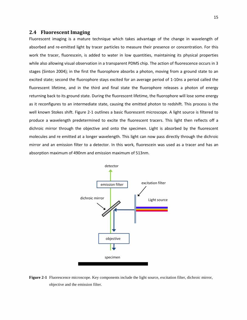
2.4 Fluorescent Imaging Fluorescent imaging is a mature technique which takes advantage of the change in wavelength of

absorbed and re-emitted light by tracer particles to measure their presence or concentration. For this

work the tracer, fluorescein, is added to water in low quantities, maintaining its physical properties

while also allowing visual observation in a transparent PDMS chip. The action of fluorescence occurs in 3

stages (Sinton 2004); in the first the fluorophore absorbs a photon, moving from a ground state to an

excited state; second the fluorophore stays excited for an average period of 1-10ns a period called the

fluorescent lifetime, and in the third and final state the fluorophore releases a photon of energy

returning back to its ground state. During the fluorescent lifetime, the fluorophore will lose some energy

as it reconfigures to an intermediate state, causing the emitted photon to redshift. This process is the

well known Stokes shift. Figure 2-1 outlines a basic fluorescent microscope. A light source is filtered to

produce a wavelength predetermined to excite the fluorescent tracers. This light then reflects off a

dichroic mirror through the objective and onto the specimen. Light is absorbed by the fluorescent

molecules and re emitted at a longer wavelength. This light can now pass directly through the dichroic

mirror and an emission filter to a detector. In this work, fluorescein was used as a tracer and has an

absorption maximum of 490nm and emission maximum of 513nm.

Figure 2-1 Fluorescence microscope. Key components include the light source, excitation filter, dichroic mirror,

objective and the emission filter.

16

3 Liquid Transport in PEMFCs and Pore Network Modeling

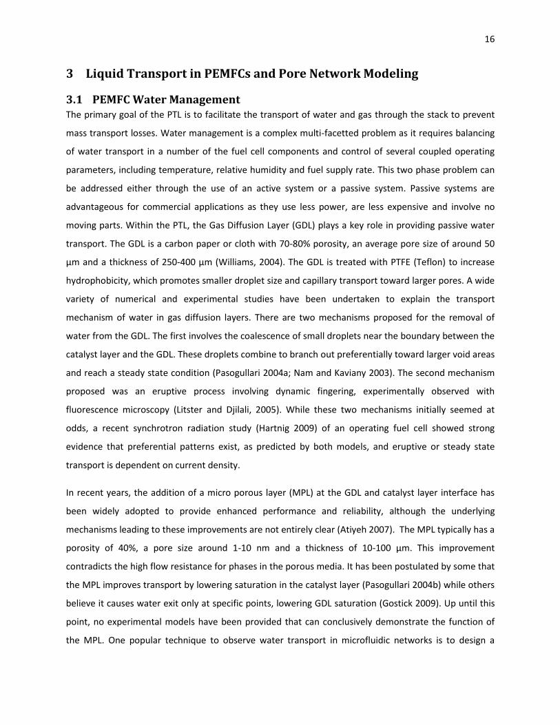
3.1 PEMFC Water Management The primary goal of the PTL is to facilitate the transport of water and gas through the stack to prevent

mass transport losses. Water management is a complex multi-facetted problem as it requires balancing

of water transport in a number of the fuel cell components and control of several coupled operating

parameters, including temperature, relative humidity and fuel supply rate. This two phase problem can

be addressed either through the use of an active system or a passive system. Passive systems are

advantageous for commercial applications as they use less power, are less expensive and involve no

moving parts. Within the PTL, the Gas Diffusion Layer (GDL) plays a key role in providing passive water

transport. The GDL is a carbon paper or cloth with 70-80% porosity, an average pore size of around 50

μm and a thickness of 250-400 μm (Williams, 2004). The GDL is treated with PTFE (Teflon) to increase

hydrophobicity, which promotes smaller droplet size and capillary transport toward larger pores. A wide

variety of numerical and experimental studies have been undertaken to explain the transport

mechanism of water in gas diffusion layers. There are two mechanisms proposed for the removal of

water from the GDL. The first involves the coalescence of small droplets near the boundary between the

catalyst layer and the GDL. These droplets combine to branch out preferentially toward larger void areas

and reach a steady state condition (Pasogullari 2004a; Nam and Kaviany 2003). The second mechanism

proposed was an eruptive process involving dynamic fingering, experimentally observed with

fluorescence microscopy (Litster and Djilali, 2005). While these two mechanisms initially seemed at

odds, a recent synchrotron radiation study (Hartnig 2009) of an operating fuel cell showed strong

evidence that preferential patterns exist, as predicted by both models, and eruptive or steady state

transport is dependent on current density.

In recent years, the addition of a micro porous layer (MPL) at the GDL and catalyst layer interface has

been widely adopted to provide enhanced performance and reliability, although the underlying

mechanisms leading to these improvements are not entirely clear (Atiyeh 2007). The MPL typically has a

porosity of 40%, a pore size around 1-10 nm and a thickness of 10-100 μm. This improvement

contradicts the high flow resistance for phases in the porous media. It has been postulated by some that

the MPL improves transport by lowering saturation in the catalyst layer (Pasogullari 2004b) while others

believe it causes water exit only at specific points, lowering GDL saturation (Gostick 2009). Up until this

point, no experimental models have been provided that can conclusively demonstrate the function of

the MPL. One popular technique to observe water transport in microfluidic networks is to design a

17

representative pore network model with properties comparable to that of the MPL. Section 3.2 provides

some porous media fundamentals while 3.3 provides a background on pore network models and their

application.

3.2 Key Terms for Analysis of Liquid Transport in Porous Media Displacement processes involving two immiscible phases in porous media have been a subject of

research for PEMFCs (Nam and Kaviany 2003) and a variety of other fields including soil hydrology

(Jerauld and Salter 1990), carbon dioxide sequestration (Ferer and Smith 2005; Kang 2002) and oil

extraction (Mann 1979). In this class of problems the upper bound of pore size is 1 mm, where surface

and viscous effects dominate. The porous materials of interest are opaque and do not permit direct

observation. Due to difficulties in performing in-situ observation, descriptive physical values of the

media have been defined to assist in understanding how these processes occur. For the movement of

phases, the porous materials resistance to fluid flow and the invading liquids behavior are of particular

interest. This section presents some basic physical properties of porous media, followed by a description

of permeability and viscosity.

Porous media can be defined as a combination of a solid and void. For the porous media of interest, the

media can be accurately described as a bulk solid minus a collection of void spheres of varying size. A

pore size is defined by the diameter of one particular void area. Generally pore sizes vary throughout

the media, and the pore size distribution is required for understanding of the porous media structure.

Pore size can be measured using mercury porosimetry (Williams, 2004). In this technique the porous

material is placed in a pressure vessel containing mercury. The ability for mercury to invade small pores

is dependent on the pore size and the applied pressure. By measuring the absorbed mercury as a

function of applied pressure, porosimetry can provide pore size distribution, total pore volume (by

integration) and total surface area. Porosity, or the total pore volume, is defined as the void space in the

media and ranges from 0 for a solid and 1 for a void volume.

While certainly not all encompassing, a pore distribution and total porosity can give a basic

understanding of the porous media structure. With information on isotropy and composition, flow

characteristics of fluids within the media may be predicted. This requires some understanding of flow

behavior in porous media. Of particular importance are flow conductance of the porous media, or

permeability, and the fluids resistance to deformation, viscosity. Typically, the solid phase is considered

inert and incompressible, and the focus is only on the invading and displaced phases. In the case of

interactions between a liquid and a gas, the system is considered two phase. There are two types of

18

processes that can occur with the interaction between a liquid and gas phase, drainage and imbibition.

In a drainage process, a wetting phase is displaced by a non-wetting phase, whereas in an imbibition

process a non-wetting phase is displaced by a wetting one. In fuel cells, under the goal of lowering

saturation, the media is treated to be hydrophobic. As it invades a dry system, this is a drainage process.

Permeability is defined as the flow conductance. It is written as

(3.2.1)

where is the permeability, refers to the pressure drop, is the dynamic viscosity and is the

superficial velocity. While the permeability is a fundamental value and is very descriptive to the behavior

of porous media, its calculation is difficult. The main approaches to find it include relying on empirical

data, using a semi heuristic approach known as the Carman-Kozeny theory, pore scale modeling of

idealized systems (typically now done with CFD) or if length scales are small enough, lattice-Boltzmann

models (Litster and Djilali, 2005).

Viscosity is the fluid resistance to either an applied shear or tensile force. A highly viscous fluid has a

higher internal resistance to changes, and compared to a less viscous fluid will respond slower.

Viscosities importance in an imbibition or drainage process lies in its relative value. A viscous fluid will

require a higher force to move and have a more damped response then a less viscous one. When a

viscous fluid invades a gas, it will invade without much resistance, as the force required for its motion is

much higher than the resistance offered by the gas. During the reverse process, the pressure on the low

viscous fluid must be very high in order to provide enough force to move the more viscous fluid. For a

fuel cell water is the non-wetting fluid and invades with a viscosity 1000x higher than air.

3.3 Modeling Techniques and Pore Network Models An excellent review was recently provided by Mukherjee (2010) that focuses on models relevant to

PEMFCs. In particular there are two main types of models used to study porous media: principle based

methods and rule based methods. Principle based methods, as the name implies, incorporate

techniques such as molecular dynamics where each individual molecule and its collisions are taken into

account. Lattice Boltzmann techniques strive for the same level of detail but reduce complexity by

simulating groups of particles that interact on a regular lattice. Computational fluid dynamics takes a

different approach by defining boundary conditions to solve fluid flow using the Navier Stokes equation.

Rule based methods are much less complex, instead creating an idealized network of the porous media

19

and requiring only simple physical rules to understand their flow processes. The main advantage of rule

based systems is that they clearly demonstrate the dominant transport mechanisms with very low

computational power, and they are easily verified by their micromodel counterparts. The most well

known rule based method is pore network modeling.

Pore network models are used to describe the behavior of drainage processes that correspond to

wetting or non-wetting fluids, respectively. The porous media is modeled as a network of

interconnected pores and throats. In this representation, contact angle, capillary number (Ca = μV/ γ or

viscous forces divided by surface tension) and relative viscosity (Vr = η1/ η2, where η1 and η2 are the

invading and displaced fluids, respectively) determine the flow characteristics. Depending on the

aforementioned dimensionless parameters three flow regimes were identified by Lenormand (1988);

stable displacement, viscous fingering and capillary fingering. Figure 3-1 shows a Log- Log map of the

invasion behavior as a function of relative viscosity (M) and capillary number.

Figure 3-1 Schematic Log Log map describing fluid flow in porous media as a function of relative viscosity (M)

and capillary number (Ca). This pore network map assumes no contact angle hysteresis or material

deformation

20

Stable displacement is the effect seen when the relative viscosity of the invading fluid is much greater

than that of the displaced fluid and the capillary number is quite high. A simple example of this type of

filling behavior can be imagined if a full glass of water is spilled onto a tabletop. The liquid spreads in all

directions, and has a continuous invasion front. Obstacles have little effect as water invades and fills

every available area. When stable displacement occurs in a bounded network with an inlet and outlet,

complete saturation of the network generally coincides with breakthrough to the outlet. Viscous forces

dominate over surface forces and the high viscosity of water controls the flooding pattern. Stable

displacement is categorized by complete filling and a continuous invasion front.

Viscous fingering occurs at similar levels of capillary number, but at low levels of relative viscosity.

Similar to stable displacement, in viscous fingering surface effects are relatively inconsequential in

comparison to viscous effects. As a fluid of low viscosity displaces that of high viscosity in the network,

interesting fractal like patterns emerge and movement of the displaced phase is directionally oriented

toward the outlet. The dead end patterns often resemble fingers, as the name suggests. As an extreme

example, consider blowing air to vacate a rigid sponge (disregard any effects due to deformation)

saturated in water. Air is forced in the +X direction toward –X. The momentum of air will be transmitted

to the water towards the –X direction, leading to some drainage. However, due to the high relative

viscosity of the water, the interface between the two fluids is unstable and some areas will vacate more

water than others. In some void spaces, water will move, while in others, it will remain. Unlike stable

displacement, where the invasion front is continuous and complete saturation occurs quickly after

network breakthrough, in viscous fingering the invasion front is discontinuous and complete saturation

is very rarely satisfied.

The last type of fluid behavior outlined in the pore network model map is capillary fingering. Capillary

fingering occurs at low superficial velocities where surface tension effects dictate chronological invasion

of the node or throat with the lowest capillary pressure (Lenormand 1990). Capillary fingering occurs at

low capillary numbers over a range of relative viscosities, although its behavior is more pronounced at

higher M values. In capillary fingering, surface forces dominate over viscous forces. Under these

circumstances, the relationship between invading fluid and the media is very important, whereas it is

largely irrelevant for stable displacement or viscous fingering. The magnitude of the pressure is given by

the Young-Laplace equation. For water displacing air in a hydrophobic media, the pressure inside the

droplet is higher than that in the network. Therefore, areas in the network with a larger radius, R,

21

require less pressure to invade and are preferentially filled first. This type of filling pattern leads to what

appears to be a non-directional filling of the largest available node(s). While capillary fingering generally

occurs only at very small length scales, low capillary numbers can also occur at correspondingly low flow

rates. One application of capillary fingering behavior is the mercury porosimetry test presented as a

method to measure porosity values. Mercury is very well known for having a very high contact angle.

When a porous media is invaded with mercury at low flow rates, it will preferentially only wet the areas

with the largest void spaces. Measuring the amount of pressure required to saturate a network with a

given change in mercury volume gives data on how many pores of a given size the network has.

Common features seen in capillary fingering behavior are non-continuous phase boundaries, trapping

and Haines jumps (1930). Non-continuous phase boundaries occur due to small nodes not being

invaded, leading to the extreme branching nature of capillary fingering. Trapping occurs when islands of

small nodes get completely surrounded by the invading phase and form stable islands (Lenormand 1983)

as they cannot be saturated or escape from the network. Haines jumps (1930) deal with the invasion

process occurring under discrete steps of burst filling in the network.

Numerical pore networks are based on reconstructed sets of two-dimensional images or advanced

techniques that extract physical properties such as porosity, pore size distribution and coordination

number from the porous media samples (Tsakiroglou and Payatakes 2000; Vogel and Roth 2001; Rintoul

1996). These parameters are then used to create a two- or three-dimensional numerical pore network. If

the expected invasion process is capillary dominated, an Invasion Percolation (IP) algorithm (Wilkinson

and Willemsen 1983), based on sequential invasion of the largest available node can be applied to

simulate the evolution of the invading phase distribution, and deduce parameters such as relative

permeability and capillary pressure (Markicevic 2007). In complex systems or regimes where multiple

modes of liquid transport can be present, such as a PEM fuel cell, current numerical pore networks lack

the complexity necessary to accurately represent the modeled media (Mukherjee 2010). One of the

most difficult aspects of pore network modeling is determining which parameters are necessary to get

an accurate representation of the modeled system. Physical experiments in the form of microfluidic

networks can augment numerical pore network results by employing the fluids of interest and directly

incorporating the relevant physical attributes of multiphase flow in micro-systems.

Microfluidic networks are physical representations of the porous media that allow direct visual

observation of the transport of the fluids of interest in a micro-structured environment. This approach

22

generally restricts the media to two dimensions, although exceptions exist (Kang 2010), and to the use

of optically transparent materials suitable for micro fabrication such as polymer or glass (Tsakiroglou

and Avraam 2002). It is important to match the relevant physical parameters such as connectivity,

contact angle, pore size, flow rate and capillary number to that of the native porous media (Blunt 2001).

If suitably matched, microfluidic networks can intrinsically include effects such as surface tension,

pinning and non-ideal surfaces that are challenging to incorporate in numerical pore network models. In

this regard, microfluidic networks provide a key tool in the study of transport in porous media.

Examples of the application of microfluidic networks include visualizing residual immiscible organic

liquids in aquifers (Conrad 1992), elucidating the role of pore network bias on water transport in fuel

cells (Bazylak 2008), and studying the effects of using non-Newtonian fluids in pore network

micromodels (Perrin 2005).

At small pore sizes, the increase in the surface-to-volume ratio and high pressures lead to additional

considerations such as contact angle hysteresis, where the act of surface wetting changes the phase

equilibrium. Hysteresis in saturation of porous media after drainage imbibition cycles is a well known

effect (Reeves and Celia 1996; Hilpert 2003) and has been previously incorporated into numerical pore

network models (Jerauld and Salter 1990). One possible cause of this effect is contact angle hysteresis,

where the receding contact angle is less than the advancing one due to nonlinear surface effects. While

the effect of contact angle hysteresis on saturation levels in cyclic invasion drainage processes is known,

it is not generally incorporated into the invasion percolation algorithm. Second, as pore sizes decrease,

capillary pressures increase and can lead to structural deformation. Low capillary pressures have been

observed to cause nanochannel collapse at small scales (Eijkel and Berg 2005), and have been

incorporated in a numerical pore network model of compacted soil (Simms and Yanful 2005). However

despite the tendency of wetted media to swell (Inglis 2005) and the influence of contact angle hysteresis

on hydrophobic surfaces (He 2004), to date no microfluidic network study has addressed the effect of

deformability or the effect of contact angle hysteresis in an invasion process.

The principal goal of this portion of the thesis was to model flow behavior in the PTL using microfluidic

techniques. However, a broader research question became apparent: Are the 3 well defined regimes of

flow behavior outlined by pore network modeling applicable to media that exhibits dynamic contact

angle effects and is deformable under pressure.

23

4 Deformability and Hysteresis in Pore Network Models

4.1 Introduction While still a relatively new technique, pore network modeling has garnered interest as a predictive

modeling tool for a variety of fields (Blunt 2001) such as: to find a relation between capillary pressure

and saturation (Vogel 2005), effective diffusivity and saturation in PEMFCs (Nam and Kaviany 2003), to

demonstrate liquid water transport in the GDL (Sinha and Wang 2007), predict effects of GDL biasing

(Bazylak 2008) and 3D visualization of invasion-percolation drainage processes (Kang 2010). Recent

numerical pore network modeling studies have applied the invasion percolation algorithm to simulate

water transport in the micro porous layer of PEM fuel cells (Wu 2010). However the application of the

invasion percolation algorithm may be inaccurate due to the very small pore dimensions (<100 nm)

encountered in the MPL.

In this study, we developed a microfluidic network approach to experimentally model the drainage

patterns that occur under low capillary number including the influence of both network deformability

and contact angle hysteresis. These experiments represent, to our knowledge, the smallest reported

microfluidic networks to date, with throats having an average hydraulic diameter of 5 μm. Flow rates

were varied to provide capillary numbers between 10-6 and 10-10, and invasion patterns and saturation

levels were recorded. This work revealed that network deformation and contact angle hysteresis can

have significant effects on the wetting patterns and saturation in small scale porous media.

4.2 Experimental Preparation Figure 4-1 shows a schematic of the microfluidic network chip as well as the network geometry and

resulting channel pattern as shown inset. The microfluidic networks were fabricated in

polydimethylsiloxane (PDMS) following standard soft-lithography procedures detailed in Chapter 2. The

channel pattern was first designed using Mathematica software. Regular square arrays were perturbed

by adding a randomly generated value from a Gaussian distribution in the x and y direction (Bazylak

2008). The mathematica code is listed in Appendix A. These arrays were imported into Autocad and

inlets and outlets were added to allow the supply and removal of liquids. These designs were sent to

Nanofab at the University of Alberta for printing of the chrome-on-glass photomasks with 1 µm

resolution. These masks were then used in the standard soft lithography technique with SU-8 2 and a

silicon wafer for the 5 µm network (Microchem, Newton Ma). Silicone elastomer base and cross linking

agent (Sylgard 184) were mixed in a ratio of 10:1. The two layers of PDMS were exposed to plasma,

24

bonded, and finally annealed for 48 hours on a hot plate at 95 C to restore hydrophobic surface

properties.

Figure 4-1 Schematic of Experimental Set up. 1st blowout shows a 4x4 randomly distributed network. The 2nd

blowout shows an SEM image of the SU-8 master at high magnification.

In order to visualize and track the water phase in the microfluidic network, fluorescein dye (Invitrogen,

Canada) was used as a tracer at a concentration of 5 µM. Flow was supplied via a syringe pump

(Harvard Apparatus, USA) with gastight 10 µL glass syringes (Hamilton, USA). Images were captured

using an inverted fluorescence microscope (Leica DMI 6000B, Germany) and 5x magnification objective

(Leica, Germany). Post processing, contrast enhancement and conversion to 8 bit were done with

ImageJ software. To quantify local channel height, relative intensities of dye were compared.

Fluorescent intensity is a function of concentration and z-axis channel height. As the solution was well

mixed, concentration of the dye is constant and any variation corresponds linearly to the change in

liquid volume.

The scanning electron microscopy image in Figure 4-1b shows edge effects that occurred in the

photoresist master. Small ripples approximately 1.5 µm apart appear along the edges and corners,

creating an irregular surface along the throats and larger nodes. Although microfabrication necessarily

introduces some structural artifacts of this nature, it is noteworthy that such multi-scale roughness

features are the norm, rather than the exception, in native porous media of interest. Experimental work

with the PDMS chips displayed significant contact angle hysteresis, an effect confirmed and well

documented in previous studies (He 2004).

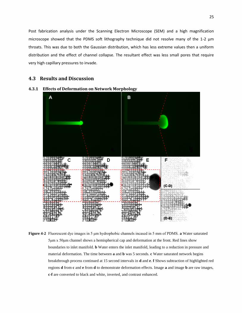
25

Post fabrication analysis under the Scanning Electron Microscope (SEM) and a high magnification

microscope showed that the PDMS soft lithography technique did not resolve many of the 1-2 µm

throats. This was due to both the Gaussian distribution, which has less extreme values then a uniform

distribution and the effect of channel collapse. The resultant effect was less small pores that require

very high capillary pressures to invade.

4.3 Results and Discussion

4.3.1 Effects of Deformation on Network Morphology

Figure 4-2 Fluorescent dye images in 5 μm hydrophobic channels incased in 5 mm of PDMS. a Water saturated

5μm x 50μm channel shows a hemispherical cap and deformation at the front. Red lines show

boundaries to inlet manifold. b Water enters the inlet manifold, leading to a reduction in pressure and

material deformation. The time between a and b was 5 seconds. c Water saturated network begins

breakthrough process continued at 15 second intervals in d and e. f Shows subtraction of highlighted red

regions d from c and e from d to demonstrate deformation effects. Image a and image b are raw images,

c-f are converted to black and white, inverted, and contrast enhanced.

26

Figure 4-2a and b show the advancement of the liquid water front into the manifold of the microfluidic

network. These images demonstrate, albeit in an exaggerated fashion, the influence of deformability

caused by capillary effects in a hydrophobic microfluidic network. Near the interface, the fluorescence

intensity is 10-fold that of the channel outside of this region. This corresponds to a height increase of

22.5 µm. It is important to note that the effect observed is due to capillary effects, and not, for

instance, photobleaching which would have the opposite effect of causing the near-interface fluid to be

dimmed (Sinton 2003). Here, as the fluid is forced into the non-wetting channel and manifold, the liquid

water deforms the channel in the vicinity of the interface. The manifold channel is much wider than it is

tall (50 µm x 5 µm) and thus expands in the out-of-plane direction.

Channel deformation in PDMS chips has been the subject of prior research (Gervais 2005), which has

found that a parabolic deflection is an appropriate first order approximation (Holden 2003). The present

images demonstrate chip deformation resulting in a four-fold increase in channel cross sectional area. In

smaller channels with aspect ratios closer to unity, as within the microfluidic network, the deformation

effect is expected to be less than that in the manifold as observed here. However, in typical capillary

fingering experiments and numerical pore network models, minute differences in channel dimensions

can lead to significant changes in the overall saturation pattern.

Figure 4-2c-e shows images of breakthrough into the outlet manifold at 15 second intervals with

evidence of chip deformation shown in Figure 4-2f. In 2c the network has just reached breakthrough. As

the expansion volume into the outlet manifold is still minute, the water pressure inside the network is

still near its maximum. In Figure 4-2d the volume of the breakthrough increases in step with a pressure

decrease of the liquid phase. In 2e the outlet volume continues to rapidly increase, and the

breakthrough volume has almost connected with other nodes in the network. The deformation of the

network is illustrated by Figure 4-2f and highlights the subtraction of the regions of interest for 2c minus

2d and 2d minus 2e. This facilitates seeing the change in intensity, or fluorescent dye content, of throats

and pores due to elastic deformation that otherwise could not be discerned. In Figure 4-2f, one can see

in the subtraction of c-d only a small decrease in intensity in the vicinity of the breakthrough. In Figure 4-

2d-e the change is much more dramatic, with an intensity decrease particularly noteworthy above the

breakthrough point. Darcy’s law for flow in porous media states that water transport occurs from

regions of high pressure to low. The decrease in intensity, without a corresponding change in saturation

of the nodes can only occur from a change in pressure due to material deformation. From intensity

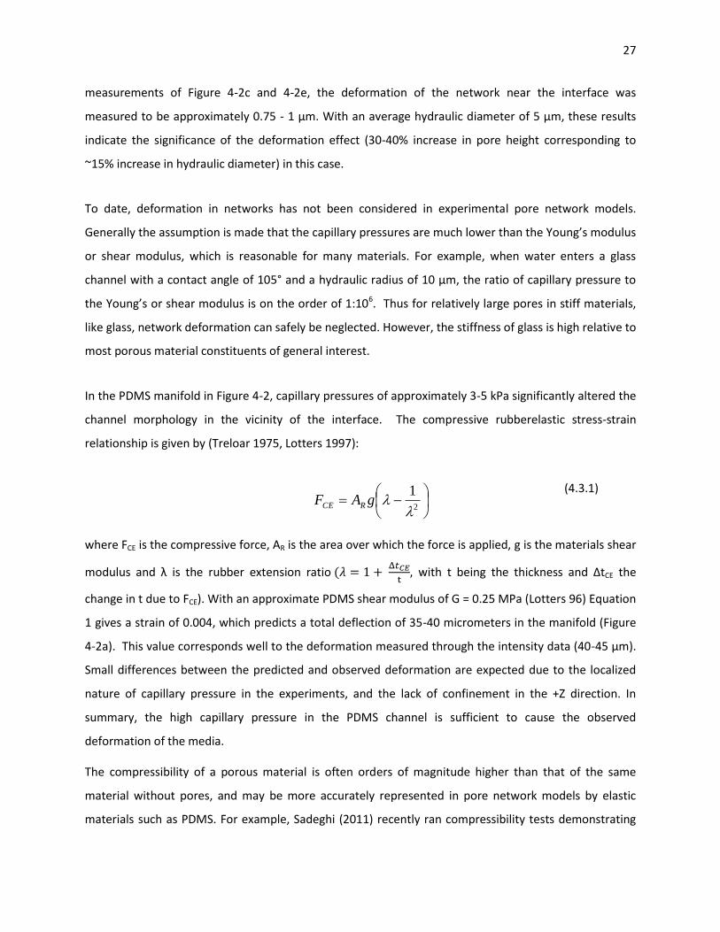
27

measurements of Figure 4-2c and 4-2e, the deformation of the network near the interface was

measured to be approximately 0.75 - 1 µm. With an average hydraulic diameter of 5 µm, these results

indicate the significance of the deformation effect (30-40% increase in pore height corresponding to

~15% increase in hydraulic diameter) in this case.

To date, deformation in networks has not been considered in experimental pore network models.

Generally the assumption is made that the capillary pressures are much lower than the Young’s modulus

or shear modulus, which is reasonable for many materials. For example, when water enters a glass

channel with a contact angle of 105° and a hydraulic radius of 10 µm, the ratio of capillary pressure to

the Young’s or shear modulus is on the order of 1:106. Thus for relatively large pores in stiff materials,

like glass, network deformation can safely be neglected. However, the stiffness of glass is high relative to

most porous material constituents of general interest.

In the PDMS manifold in Figure 4-2, capillary pressures of approximately 3-5 kPa significantly altered the

channel morphology in the vicinity of the interface. The compressive rubberelastic stress-strain

relationship is given by (Treloar 1975, Lotters 1997):

2

1

gAF RCE

(4.3.1)

where FCE is the compressive force, AR is the area over which the force is applied, g is the materials shear

modulus and λ is the rubber extension ratio

with t being the thickness and ΔtCE the

change in t due to FCE). With an approximate PDMS shear modulus of G = 0.25 MPa (Lotters 96) Equation

1 gives a strain of 0.004, which predicts a total deflection of 35-40 micrometers in the manifold (Figure

4-2a). This value corresponds well to the deformation measured through the intensity data (40-45 µm).

Small differences between the predicted and observed deformation are expected due to the localized

nature of capillary pressure in the experiments, and the lack of confinement in the +Z direction. In

summary, the high capillary pressure in the PDMS channel is sufficient to cause the observed

deformation of the media.

The compressibility of a porous material is often orders of magnitude higher than that of the same

material without pores, and may be more accurately represented in pore network models by elastic

materials such as PDMS. For example, Sadeghi (2011) recently ran compressibility tests demonstrating

28

Teflon treated PEMFC gas diffusion layers undergoing an elastic strain of 0.08 under a force of only 0.15

MPa. Figure 4-3 shows a stress-strain curve from this work with a linear fit for strains under 0.1.

Figure 4-3 Stress-Strain data from Sadeghi (2011) with a fit for points below a strain of 0.1 to approximate the

linearized region.

In a 50 µm x 5 µm pore and the same contact angle and capillary pressure as in PDMS example, the

deformation in this gas diffusion layer would be approximately 20 micrometers. And in the microporous

layer of PEMFCs, sub 100nm length scales (Tang 2006; Chun 2010) correspond to invasion pressures that

approach 1 MPa. Other media such as sandstone and soils are well known for their low compressive

strengths (Bell 1997), and it should be expected that invasion of small pores by a non-wetting fluid will

result in strong capillary pressures and deformation in these materials. In cases such as these, our

results indicate that deformation can have a strong effect on the local pore morphology, and the

resulting filling dynamics.

0.0 0.5 1.0 1.5Pc MPa0.0

0.1

0.2

0.3

0.4

0.5

Strain t to

Linearized Stress Strain Curve for TGP H 060, to 0.19mm

29

4.3.2 Effects of Contact Angle Hysteresis on Network Saturation

Figure 4-4 Images showing the effect of hysteresis on the contact angle of water invading the PDMS network.

Dotted line indicates the approximate contact point between the liquid and the walls. a Liquid water was

introduced into a 10 µm x 10 µm channel. The contact angle can be seen to be approximately 105°, as

the meniscus is in front of the wetted perimeter. b When flow is reversed the liquid water meniscus

retreats, corresponding to a contact angle around 85°

Contact angle hysteresis is also expected to play a role in two-phase transport in common porous

materials. Figure 4-4 shows the effect of contact angle hysteresis that occurs when water invades a

pristine hydrophobic PDMS channel. In Figure 4-4a, liquid water was entered into a 10 µm x 10 µm

channel at correspondingly low flow rates. Once invasion into the channel occurred, fluid pumping was

stopped, and equilibrium was allowed to be reached. It can be seen that the meniscus of the water is

clearly bulging forward, indicative of a contact angle greater than 90°. At this point the flow of liquid

water was reversed to measure the receding contact angle prior to drainage. Figure 4-4b was taken

approximately 60 seconds after Figure 4-4a and corresponds to a contact angle of approximately 85°.

These measurements indicate a strong contact angle hysteresis transition from hydrophobic to

hydrophilic.

30

Although much more sophisticated approaches to contact angle measurements on a flat surface are

available (Lin 1996), these methods do not consider non-homogenous surfaces or the effects of

confinement as in pore networks. The results in Figure 4-4 confirm that PDMS microchannels exhibit

significant contact angle hysteresis, and deviation from results that do not consider this effect are to be

expected. Specifically, in a network exhibiting significant hysteresis, pores will not vacate unless negative

gauge pressures are applied.

Figure 4-5 Microscopy images showing invasion into a hydrophobic network at a capillary number of 10-6

. a

Invasion begins at a single node that branch into the network. b Saturation proceeds toward the bulk

network bulk and outlet. c Large scale localized saturation can be seen as breakthrough occurs. d

Breakthrough and saturation along the outlet manifold leads to saturation back into the network. All

images converted to black and white, inverted, and contrast enhanced.

Figure 4-5 shows the wetting pattern into a microfluidic network at flow rates corresponding to a

capillary number of 10-6. Such low capillary numbers indicate that capillary effects dominate over

viscous forces, and in non-wetting media the invasion of small pores is highly unfavorable. The expected

wetting pattern is thus capillary fingering with low total saturation. In Figure 4-5a, the wetting begins at

the widest channel in the network, second from the top on the left side of the network. The invasion

occurs along a single line of throats and nodes, before expanding into the network (Figure 4-5b).

31

Invasion occurs in a stepwise manner, with the largest pores being invaded first (as expected with

hydrophobic media), however through the filling process even the smallest pores are filled with no

detectable receding. The resulting wetting pattern corresponds to effectively complete localized

saturation. Despite a significant pore size distribution, there is no evidence of a capillary fingering

behavior or trapping as predicted by classical theory. In Figure 4-5c, this expansion continues and

breakthrough occurs into the outlet. It is worthwhile to note that fluorescent dye enters the network

from only two nodes. Breakthrough occurs at a single node but quickly extends to multiple nodes at the

outlet side. It is also interesting to observe back diffusion occurs from the outlet side into the network.

This can be seen by comparing network saturation in Figure 4-5c and 4-5d along the outlet. We attribute

this back diffusion to the decrease in volume of the nodes at breakthrough, as previously explained. This

local network volume change leads to a temporarily higher flow rate at the outlet, and additional

invasion. Together, these results indicate higher saturation than expected for such a low Capillary

number invasion, no receding of nodes or throats following breakthrough and no observable trapping.

All of these attributes are in contrast to filling dynamics predicted by classical theory.

32

Figure 4-6 Fluorescent dye images of a hydrophobic network invaded at flow rates corresponding to a capillary

number of 10-10

. In a invasion occurs along a single row of nodes toward the outlet. In b the invasion

then branches in the two lateral directions and two separate invasion points enter the network. c

Invasion points consolidate and multiple trapping events can be identified. d Breakthrough occurs.

Trapping events seen in c have disappeared and new ones have formed. Time between images was, in

order, 12 minutes 30 seconds, 21 minutes 30 seconds and 46 minutes 50 seconds. Images were

converted to black and white and contrast enhanced.

Figure 4-6 shows invasion into a segment of a microfluidic network under a capillary number of 10-10,

four orders of magnitude lower than the corresponding results of Figure 4-6. In a sample that exhibits no

33

contact angle hysteresis or deformation, the expected invasion pattern would be pure capillary fingering

behavior. That is, the liquid water would fill in finger patterns with large areas including trapped air.

However, as in Figure 4-6, the wetting pattern was not indicative of the classic behavior. Figure 4-6a and

4-6b show expansion into a large volume throat and the contact angle hysteresis that prevents receding

from the surrounding narrow nodes. Figure 4-6c and 4-6d show network invasion at later time steps.

Saturation again occurred in a step-wise movement of bursting invasion and then periods of no flow and

pressure buildup. In the bottom portion of Figure 4-6c and 4-6d, evidence of trapping can be seen. The

small areas trapped in 4-6c were eventually invaded over time as seen in 4-6d. It is expected that these

small saturation changes occurring over longer times are due to a combination of PDMS gas

permeability and corner flow. Corner flow was observed in a previous study (Lenormand and Zarcone

1985) which attributed this effect to an increase in saturation at lower capillary numbers. This work is

differentiated from ours in that it studied the behavior of air displacing oil, wherein the air never fully

wetted the channels, the oil exhibited negligible contact angle hysteresis, and no material deformation

was present.

4.3.3 Modifications to the Invasion Percolation Algorithm

As detailed above, invasion patterns observed in these tests deviate significantly from those predicted

from the established invasion percolation algorithm (Wilkinson and Willemsen 1983). The two large

differences between this study and the invasion algorithm for capillary fingering are the contact angle

hysteresis and the deformable nature of the media. The algorithm is based on an idealized liquid

behavior in porous media with no contact angle effects and very high modulus to study the isolated

effects of relative viscosity and capillary number on liquid invasion in a non-wetting media. The

differences between this algorithm and the study in this media are exacerbated by the small pore sizes,

elastomeric material and dynamic contact angle effects.

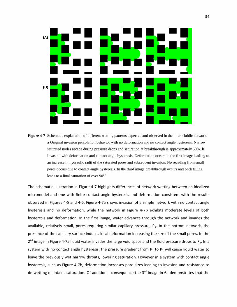
34

Figure 4-7 Schematic explanation of different wetting patterns expected and observed in the microfluidic network.

a Original invasion percolation behavior with no deformation and no contact angle hysteresis. Narrow

saturated nodes recede during pressure drops and saturation at breakthrough is approximately 50%. b

Invasion with deformation and contact angle hysteresis. Deformation occurs in the first image leading to

an increase in hydraulic radii of the saturated pores and subsequent invasion. No receding from small

pores occurs due to contact angle hysteresis. In the third image breakthrough occurs and back filling

leads to a final saturation of over 90%.

The schematic illustration in Figure 4-7 highlights differences of network wetting between an idealized

micromodel and one with finite contact angle hysteresis and deformation consistent with the results

observed in Figures 4-5 and 4-6. Figure 4-7a shows invasion of a simple network with no contact angle

hysteresis and no deformation, while the network in Figure 4-7b exhibits moderate levels of both

hysteresis and deformation. In the first image, water advances through the network and invades the

available, relatively small, pores requiring similar capillary pressure, P1. In the bottom network, the

presence of the capillary surface induces local deformation increasing the size of the small pores. In the

2nd image in Figure 4-7a liquid water invades the large void space and the fluid pressure drops to P2. In a

system with no contact angle hysteresis, the pressure gradient from P1 to P2 will cause liquid water to

leave the previously wet narrow throats, lowering saturation. However in a system with contact angle

hysteresis, such as Figure 4-7b, deformation increases pore sizes leading to invasion and resistance to

de-wetting maintains saturation. Of additional consequence the 3rd image in 6a demonstrates that the

35

pressure drop at breakthrough to the outlet prevents back diffusion into the network. In 6b however,

the elastic response of the media and non-instantaneous pressure drop consistent with observations

detailed earlier lead to a higher fluid pressure after breakthrough and invasion into the network from

the outlet manifold. Figure 4-7 illustrates the effect of deformation normalizing the pore geometry

locally at the interface and an increase in fluid saturation compared to conventional theory. The net

result is that more throats are filled than would be filled in a stiff network with no contact angle

hysteresis. These results are explained by the combination of two effects: (1) Deformation locally

increases the size of near-interface pores, increasing filling rates; and (2) Contact angle hysteresis serves

to prevent subsequent drainage of pores once filled. The combined effect is an increase in local

saturation and subsequent increase in total saturation than would otherwise be expected.

4.4 Summary Experimental pore network models can isolate the dominant processes which characterize the media,

allowing one to extrapolate effects at the microscale involving relative viscosity and capillary number to

the bulk media. At small pore scales the increase in the surface-to-volume ratio and high pressures lead

to additional factors in governing saturation and invasion patterns. Using custom designed experimental

pore networks, a study was conducted to investigate the effects of contact angle hysteresis and

deformable media. Our networks utilize the smallest reported pore sizes to date, with an average

hydraulic radius of 5 µm. We demonstrate chip deformation due to the increase in invasion pressures to

Young’s modulus of the host media, leading to a 15% increase in the hydraulic radii of throats. The

effects of contact angle hysteresis, where saturation of narrow throats is maintained despite large

pressure drops at breakthrough are also documented. At capillary numbers (10-6 - 10-10) for which

conventional theory would predict low saturation, we report values approaching complete saturation

(>95%). We attribute these differences to the use of media and liquids that are susceptible to

deformation and contact angle hysteresis. We characterize a revised percolation behavior for networks

sharing these properties. This work has application to predicting and modeling liquid invasion in porous

media with contact angle hysteresis or a low ratio of modulus of elasticity to invasion pressures at small

pore sizes.

36

5 A Micro Bubble Fuel Cell (ACDCμFC)

5.1 Introduction While high costs stand in the way of automotive fuel cells, microfuel cells have a significantly lower

barrier due to a higher price point. For example, 1 gram of gasoline has a specific heat of combustion of

around 12.5 watt hours. There are approximately 730 grams in a litre of gasoline, which in Canada

currently costs between $1.20- 1.40. So for gasoline you can get roughly 12.5 watt hours for 0.2 cents. A

single disposable AA battery has a mass of over 20 grams and costs approximately $5. The available

energy is around 4 watt hours. The same amount of energy as a gram of gasoline in AA batteries costs

$15. This equates to a 4 order of magnitude difference in the price/ Watt hour between gasoline and

batteries.

Aside from the much higher price point in portable electronic devices, fuel cells also hold an advantage

in energy density over batteries. A typical AA battery provides only 4 watt hours/ 20 grams, and future

projections do not expect significant increases in energy/mass or volume. Fuel cells, on the other hand,

can use energy dense fuels capable of energy densities an order of magnitude higher than batteries

(Dyer 2002). Recently there has been an increased consumer demand for lightweight cell phones and

laptop computers that can operate off the grid for extended periods. The higher price per unit energy

that consumers are willing to pay, coupled with the capability of high energy density, have made fuel

cells the focus of research from a variety of companies including startups (Angstrom power) and large

traditional electronic firms (Samsung). The majority of current research for commercial application has

been on scaled down traditional fuel cells, such as the PEMFC or, a variant, the direct methanol fuel cell

(DMFC). Over the last 10 years, the microfluidic fuel cell has been introduced. It has been designed from

the “bottom up”, taking advantage of microscale flow phenomena to limit or discard components of

traditional fuel cells.

The original and most common type of microfluidic fuel cell (Ferrigno 2002) is the laminar flow fuel cell

(LFFC). In this type of fuel cell, liquid fuel and oxidant flow parallel down a single channel. A schematic of

an LFFC is shown in Figure 5-1. Liquids are provided from the top and electrodes are placed on side

walls. Due to the length scales and flow rates, mixing is diffusion limited, and fuel crossover is restricted

to the interfacial area. The liquids allow ion transport, but prevent electronic conduction, which occurs

through an external circuit. The functions of a membrane in a typical fuel cell are accomplished by the

laminar flow, eliminating the need for this expensive component. The LFFC also has reduced complexity,

37

as it only needs (beyond external pumping) a single channel and two electrodes. The potential energy

density is theoretically very high, approaching that of pure fuel and oxidant.

Figure 5-1 Schematic of a laminar flow fuel cell. Liquid fuel and oxidant are pumped separately from the top. Due

to the low Reynolds number, the fluid behavior is laminar and mixing is diffusion limited. Electrodes

are placed at the side to draw current, and ions travel across the two liquids in the horizontal direction.

Mass transport effects cause depletion regions to form at the anode and cathode, and non-reversible

mixing occurs at the fuel and oxidant boundary.

The first LFFC had poor energy density and a fuel utilization of only 0.1%. Limitations with the original

design were due to mass transport effects caused by low diffusion rates on the anode and cathode, and

poor reactivity of the oxidant. Future generations of LFFC involved a variety of different fuel, oxidants

and electrode placements and geometries to improve performance. Kjeang (2006) radically decreased

diffusion distances by applying porous flow through electrodes. This gave the highest reported fuel

utilization (>99%) and power density (131 mW/cm2) to date. Mitrovski (2004), (Mitrovski and Nuzzo

2006) and Jayasharee (2005; 2006) employed an air breathing system to solve the problem of poor

oxidant reactivity and transport. In this case, air diffused through a thin gas diffusion layer or PDMS

membrane onto a cathode. While lowering the required pumping power and improving oxygen

transport, design restrictions and tradeoffs shared with standard LFFCs limit peak performance.

38

All LFFCs are limited by some combination of the following factors; mixing and contamination, mass

transport effects, low fuel utilization and high ohmic resistances. Mixing and contamination are caused

by diffusion between the fuel and oxidant. Once this mixing occurs, a diffusion zone of fuel and oxidant

is formed and cannot be used. There are also constraints on flow speed and geometry to prevent fuel

and oxidant from diffusing to the opposite electrodes. Mass transport effects in LFFCs are also strongly

affected by diffusion. As described earlier, mass transport causes a sharp loss in fuel cell efficiency when

reactants in the vicinity of an electrode are depleted. In laminar flow fuel cells, species transport is

diffusion limited. This causes depletion regions to form around the electrodes, starving the cell. While

reducing the laminar flow characteristics of the cell would decrease mass transport losses, this comes at

the expense of increased mixing between fuel and oxidant. Combined with the relatively short depletion

region formed near the electrodes, the effect of mixing and mass transport losses cause a >90% of the

fuel to be unused in typical LFFCs. Another important source of inefficiency in LFFCs is ohmic losses. The

goal of LFFC research is to demonstrate the capability of energy densities beyond those possible with

batteries. This has led to most work using energy rich fuel and oxidants, such as methanol and hydrogen

peroxide. Unfortunately these types of liquids are not particularly well suited for ionic conduction. This

causes the LFFC to have large ohmic losses at high currents. Reducing the distance between electrodes,

the simplest way to reduce cell resistance, is not possible due to fuel and oxidant mixing. In general

LFFCs are limited by interconnected factors that relate to species transport and ohmic losses.

One way to address some of the shortcomings of current LFFC technology, proposed here, is to employ

gaseous fuel and oxidants separated by a liquid phase. This type of fuel cell would use the phase

boundaries instead of laminar flow as a membrane. This could have a variety of positive impacts on the

aforementioned limitations of the LFFC. The fuel and oxidant stay separate throughout the system,

eliminating fuel crossover. This gives freedom to the fuel cells geometric design, including one capable

of producing AC power. With respect to mass transport limitations, 2 phase slug flow in microchannels

enhances mixing (Song 2003) and gaseous fuels have diffusion rates approximately 3 orders of

magnitude higher than liquids. Ionic conduction occurs between electrodes through the liquid phase,

which is independent of fuel and oxidant, and can be selected to have high ionic conductivity.

While the use of fuel and oxidant bubbles in a fuel cell is a new paradigm for micro fuel cells, two-phase

flow has been a growing research field in microfluidics for over 10 years. Recent advances include

understanding the mechanisms of droplet and bubble formation into a single liquid channel (Garstecki

2005), and compiled flow regime maps showing gas behavior in liquid as a function of flow velocities

39

(Gunther and Jensen 2006). Bubbles of single composition in microchannels have been recently applied

to novel applications including message encoding (Hashimoto 2009) and as bits for computational

operations (Prakash and Gershenfeld 2007). Alternating droplets of an immiscible oil phase in aqueous

solution were first demonstrated by Zheng (2004) at various flow rates. More recently, Hung (2005)

used modified T channels that lowered flow instability and demonstrated the capability to vary the ratio

of alternating droplets. However, no one to date has applied these techniques to produce bubbles of

alternating composition in a single microchannel. Furthermore, no work in two phase microfluidic

research has employed bubbles to produce voltage or draw energy.

In this work, we develop the groundwork for micro bubble fuel cells that produce either AC or DC

power. We demonstrate feasibility by producing an open circuit voltage of 1.03V and a current of 0.2

µAmps. To our knowledge these experiments represent the first; microfluidic chip that produces

bubbles of alternating composition in a single microchannel; microfluidic fuel cell that uses bubbles as

fuel and oxidant carriers; fuel cell capable of generating alternating current.

5.2 Classification of Microfluidic Bubble Fuel Cells There are three types of microfluidic bubble fuel cells that were conceptualized in this thesis. Each of

these fuel cells will be presented in detail. Type 1 was designed to create a microfluidic bubble fuel cell

capable of reversible operation. Type 2 uses an external supply of hydrogen and oxygen and unique

configuration capable of producing AC power. Type 3 is similar to Type 2, but it uses parallel channels of

fuel and oxidant bubbles separated by a wall. The Type 3 bubble fuel cell produces DC power.

5.2.1.1 Type 1

The Type 1 bubble fuel cell was designed for reversible operation, with fuel and oxidant being created in

situ. A schematic of the Type 1 microfluidic bubble fuel cell is shown in Figure 5-3a, and an image of the

manufactured chip is in 5-3b. Figure 5-3a shows the reversible operation of the Type 1 bubble fuel cell.

T1 shows the initial system, a filled channel with gold plated electrodes along the bottom. At T2 a battery

is used to electrolyze a hydrogen and oxygen bubble on two of the electrodes. At T3 fluid flow moves the

two bubbles down the channel over another pair of electrodes. If the electrical connection is closed,

current will flow. If sequences of bubbles are electrolyzed, fluid movement could change the output

polarity. The components of the microfluidic bubble fuel cell are a single channel PDMS chip with inlet

and outlet ports on a patterned gold slide. The gold acts as the electrode for both reduction and

oxidation. The Type 1 ACDCμFC led to measured voltages and through image analysis, current and

power data. However, for reasons that will be discussed, research is now focused on the Type 2.

40

Figure 5-2 Schematic and image of a Type 1 micro bubble fuel cell.a T1 shows the initial system, which is a single

channel with gold electrodes on the bottom. At T2 a battery is used to electrolyze the electrolyte,

producing hydrogen and oxygen. At T3 fluid flow through the system moves the bubbles down the

channel, and current can be drawn. b is an image of the actual device rotated 90° compared to a. The

entire microbubble fuel cell fits on a 25mm x 75 mm glass slide.

5.2.1.2 Type 2

The Type 2 fuel cell is designed to operate with fuel and oxidant supplied externally. By applying

microfluidic techniques to create alternating droplets, the Type 2 FC uses a bubble train of fuel- liquid

electrolyte – oxidant – liquid electrolyte. This configuration is transported across static electrodes

resulting in an AC voltage. Figure 5-2 shows a schematic for the proposed microfluidic bubble fuel cell

(the AC DC micro fuel cell, or ACDCμFC). Figure 5-2a shows the reaction kinetics involved with hydrogen

and oxygen in alkaline media. The bubbles are denoted by the light blue and tan, and the electrodes sit

underneath the bubbles. A blue electrode corresponds to an oxidation reaction and red to a reduction

reaction. Figure 5-2a refers to time T1 in 5-2b, which shows the effect of the bubble train flow on the cell

behavior. In Figure 5-2b, fluid flow from the left causes the sequence of bubbles to move to the right. At

time T2, the fuel and oxidant are now in-between electrodes and no current or voltage is generated. At

T3 the hydrogen bubble of T1 is now at the electrode that reduced oxygen in T1 and a new oxygen bubble

is at the first electrode. This alternation continues indefinitely and the speed of alteration is dependent

on the fluid flow rate. An idealized curve showing voltage as a function of time is in 5-2c. It shows that at

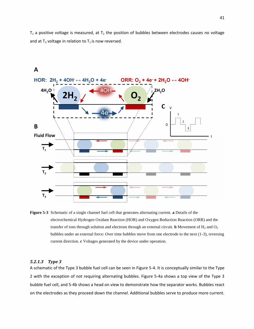
41

T1 a positive voltage is measured, at T2 the position of bubbles between electrodes causes no voltage

and at T3 voltage in relation to T1 is now reversed.

Figure 5-3 Schematic of a single channel fuel cell that generates alternating current. a Details of the

electrochemical Hydrogen Oxidant Reaction (HOR) and Oxygen Reduction Reaction (ORR) and the

transfer of ions through solution and electrons through an external circuit. b Movement of H2 and O2

bubbles under an external force: Over time bubbles move from one electrode to the next (1-3), reversing

current direction. c Voltages generated by the device under operation.

5.2.1.3 Type 3

A schematic of the Type 3 bubble fuel cell can be seen in Figure 5-4. It is conceptually similar to the Type

2 with the exception of not requiring alternating bubbles. Figure 5-4a shows a top view of the Type 3

bubble fuel cell, and 5-4b shows a head on view to demonstrate how the separator works. Bubbles react

on the electrodes as they proceed down the channel. Additional bubbles serve to produce more current.

42

The Type 3 bubble fuel cell has improved conductivity over the Type 2. This is because ion conduction is

perpendicular to the flow of bubbles, allowing a much larger effective cross sectional area. The Type 3

bubble fuel cell has been designed but not yet fabricated. Testing is expected to start in late July- early

August.

Figure 5-4 Schematic of a Type 3 micro bubble fuel cell. a gives a top view of the system. Gas slugs enter into the

channels through T junctions. Fuel and oxidant travel down independent channels over electrodes. A

PDMS barrier provides a separator. b clarifies the setup with a down the line view, showing the bubbles

in the channel, electrodes on the bottom and separator.

5.3 Experimental Preparation Experimental preparation to create the microfluidic bubble fuel cells followed many of the same

techniques as the pore network modeling study. Microfluidic networks were fabricated out of PDMS and

followed standard soft lithography procedures. Networks were designed in Autocad and transparencies

were produced by Fineline Imaging (CO, USA). SU-8 100 was used and for all of the bubble fuel cells, spin

speeds of 2000 rpm were used to create networks with a z-axis height of 100 μm.

To reduce costs and fabrication time, gold slides were etched as electrodes. Gold slides are glass slides

with a thin, (~50 μm) layer of chromium and gold. The gold etching process involves covering the desired

electrode pattern, etching the gold and chromium away and then removing the covering. The technique

to accomplish this involves using SU-8 in the identical manner as silicon master preparation. For gold

slides, SU-8 25 is spun on at a speed of 2000 rpm. Pre and post baking times are 3 minutes at 65° C and 5

minutes at 95° C. Exposure is for 50 seconds. After the SU-8 layer has been developed on the gold slide,

separate gold and chromium etches are applied. The wafer is then cleaned with IPA and placed in PG

Remover (Microchem, USA), a strong solvent.

43

The gold slide and PDMS mold were bonded using the plasma cleaner described in Chapter 2. Low

pressure inlet port seals were created out of PDMS. The plasma cleaning process does not allow PDMS

and gold to bond. In some cases, this led to no change in the chip performance, in other chips significant

leakage would occur along the electrodes. In chips where leakage was problematic, clamping was

accomplished with an independently designed PMMA case.

The conductive solution was 1M KOH. This was prepared by adding KOH crystals to water. The channel

dimensions were large enough that unaided visual observation and digital recording were possible. To

improve clarity, a colorant was added to the liquid. It was found that surface effects could cause pinning

and high surface tension effects counteracted bubble formation. To decrease these surface effects,

various amounts (0.1 wt% - 0.01 wt%) of Tween 20 were added to the solution.

For the Type 2 fuel cell, hydrogen was the fuel and ambient air was used as the oxidant. Both were

supplied with 1ml gas tight syringes (Hamilton, USA). Syringes were filled with hydrogen through a

specially designed filling station. Flow rates of both liquid and gas were provided with syringe pumps

(Harvard Apparatus, USA) and varied between 5 and 50 μL/min.

5.4 Results and Discussion

5.4.1 Type 1

The Type 1 bubble fuel cell provided reversible operation, an open circuit voltage of over 1.03 V and an

inferred current from images of approximately 1.5 μAmps. This work showed the viability of the bubble

fuel cell. However, a variety of shortcomings in the operation of the Type 1 (that should not exist in the

other bubble fuel cells) prevented further work.

The first tests with the Type 1 bubble fuel cell involved 1M KOH in the single channel with no surfactant.

It was found that the electrolyzed bubbles coagulated and drifted into the electrolyte, eliminating the

needed spacing between fuel and oxidant. To prevent this effect, Tween 20 was added to the KOH.

Small doses seemed to improve performance by forming larger stable bubbles on the electrodes.

However, once these bubbles were pushed with a fluid to move them down the channel, pinning on the

metal surface prevented smooth movement of the gas phase. The electrolysis reaction creates twice the

number of hydrogen molecules as oxygen molecules, and the bubbles had different resistances to the

fluid flow. This asymmetric bubble growth altered the spacing, and in some cases led to merging. To

reduce the pinning and bubbles resistance to flow, additional Tween 20 was added to the liquid. While

the Tween 20 improves the bubble behavior, it ruined the electrolysis process by producing countless

44

small bubbles on the gold electrodes. The best case scenario for surfactant dosage was to provide as

much as possible without preventing single bubbles of hydrogen and oxygen to evolve on the

electrodes. Another technique to eliminate unequal movement of bubbles down the channel was to use

three electrodes to produce Hydrogen – Oxygen – Hydrogen. The goal was that as the oxygen electrode

evolves half as much gas as hydrogen, this arrangement would produce close to equal sized bubbles on

all 3 electrodes. While this helped produce similarly sized bubbles, bubble pinning behavior still

occurred. Managing bubble evolution and controlling bubble movement in the Type 1 fuel cell was

difficult.

Figure 5-5 Images taken at closed circuit to infer current in a Type 1 bubble fuel cell. Image b was taken 80

seconds after Image a. The flow rate is 0, electrolyte 1M KOH. Analysis of the decrease in bubble size

corresponded to a current of 1 μAmp.

Figure 5.5 shows two images of the type 1 fuel cell taken 80 seconds apart. Images of the system left at

closed circuit for extended periods of time were used to measure the change in bubble volume, and

calculate current. This technique found a current of 1.5 μAmps. One direct measurement with an

ammeter registered a spike of 0.2 μAmps. A peak open circuit voltage of 1.03 was measured in a

separate test. This experiment had no Tween 20, and the open circuit voltage decreased significantly.

With Tween 20, the highest measured voltage was 0.6V.

5.4.2 Type 2

A few different designs to produce bubble alteration for the type 2 fuel cell were attempted. The

original setup was a double T junction with equal cross sectional areas. An example of this type of

network can be seen in Zheng (2004). However it was found that this caused the fuel and oxidant to

often merge, leading to mixing. To avoid this, a new design with a narrowed neck was employed. A

45

sequence of images showing alternate bubble formation with this design can be seen in Figure 5-6. In

Figure 5-6a stream of air from the right reservoir has a large enough pressure to displace the fluid and

enter the main channel. In part b the gas phase blocks off the entire channel and a small liquid barrier

between the opposing gas prevents any contamination. In c this barrier between the gases increases

because fluid flow is blocked from going downstream and instead enters the opposite gas channel. In d,

the buffer reaches is maximum length and the liquid is at high enough pressure to snap off the gas slug.

The gas slug breaks free in Figure 5-6e and moves downstream. In 5-6f the pressure from the left gas

channel now has enough pressure and injects into the main channel. While in Figure 5-6 the system

successfully injects bubbles of alternating composition, and this design was an improvement over the

first attempt, the overall reliability of this system is quite poor.

Figure 5-6 Sequential images of alternating bubble creation in a double-T junction. a Stream of air from right gas

reservoir enters the main channel. b Invading fluid squeezes off entire channel, a small liquid barrier

prevents mixing with opposite gas channel. c-d Liquid fluid, blocked off from the main downstream

channel, enters the opposing gas channel, increasing buffer width. e Gas segment separates from right

46

gas reservoir and moves downstream. f Pressure from liquid entering the left gas channel stops, air from

left gas reservoir enters main channel. Blowouts added for detail.

This is believed to be due to pressure instabilities. The narrowing of the neck before entering the liquid

was designed to encourage liquid wetting and to increase the gas pressure threshold to burst, like a

piston, into the liquid phase. In operation, however, the narrowing of the neck and its dependence on

the other gas injection channel destabilized the system. For example, consider a single T junction with

this narrowing design in operation. As the gas pressure builds up, the gas-liquid meniscus moves closer

and closer to the main injection point. Once a certain pressure is overcome, the gas invades, and once

the pressure of the liquid behind increases sufficiently it gets clipped off. With a double T junction, there

is the additional component of what is occurring in the opposite gas injection point. If the two gas

channels are increasing in pressure and pushing on the narrowing neck toward the main channel

simultaneously, the one that invades the main channel first will create a high pressure on the other. This

has been observed to break seals and cause pressure leakage, or cause the non-firing injection channel

to respond by producing two or more slugs in a row.

To reduce this effect a T junction with a bowtie shape (Hung 2005) from previous alternating droplet

work was employed. The goal of this system is to form a large meniscus between the liquid and gas near

the main channel providing stability. An image of the new mask design, with the matching electrode

mask is provided in Figure 5-7a.

Figure 5-7 a Autocad design for the “bowtie” T channels and mask for the gold electrode layer. The mold from the

top mask fits directly on top of the gold electrode. The dimensions of both of these chips are 25mm x

75mm. The switchback area is where bubbles of alternating composition will produce an AC voltage. b

Image of a test system (narrowing neck) with no electrodes. Used to test capability of generating

alternate slugs

47

Figure 5-7b shows a test version of the Type 2 cell. Switchbacks are used to increase the amount of

bubbles on each electrode and increase electrical output. To produce AC current in a chip with this

design requires that the gas and liquid slugs are consistently sized. Also, if the slugs are too small, they

will not be properly spaced on the electrodes during operation and will not react. On the other hand, if

they are too large, they may be on both electrodes at once, and again no reaction will occur. A variety of

different flow rates were tested to create consistent sized slugs. Figure 5-8 demonstrates the ability to

create consistent gas and liquid slugs at a flow rate of 25 μL/min for the liquid and 15 μl/min for each

gas injection point. To date there have been no measurements of voltage or current with the Type 2

bubble fuel cell. This is due to reliably in creating bubbles of alternating composition in the single

microchannel.

Figure 5-8 Test chip demonstrating consistent gas/liquid slug sizes. Flow rates were 25 μl/min for the liquid and 15

μl/min for each gas.

48

5.5 Summary Micro bubble fuel cells were proposed to address the drawbacks of laminar flow fuel cells, namely low

fuel utilization, mass transport limitations and ohmic losses. The use of bubbles offers a variety of

advantages including a phase barrier between electrolyte and fuel, higher rates of diffusion, an

independently chosen electrolyte and the potential for AC operation. Work with bubble fuel cells

resulted in a measured open circuit voltage of 1.03 volts and a current measurement of 0.2 µAmps.

Potential benefits of bubble fuel cells include reversible operation and multiple passes of fuel to improve

utilization. Additional research is required to address surfactant use, control over bubbles in

microchannels and dual T junctions to achieve AC operation.

49

6 Conclusions and Future Work In this thesis microfluidic techniques were applied to understand the effects decreasing length scales

and non-ideal media on liquid invasion in pore network models and to create a new type of micro fuel

cell. To study the effects of deformation and contact angle hysteresis we developed and tested the

smallest pore network model to date, with an average hydraulic radius of 5 μm. We demonstrated that

deformation causes a normalization of small pores and contact angle hysteresis prevents a decrease in

saturation at breakthrough. This work is important for future applications of pore network modeling on

media sharing these properties. For the micro fuel cell, we introduce the concept of using bubbles as

carriers of fuel and oxidant. Depending on the design and operation of this class of fuel cell, AC or DC

current can be produced. This research is the first to report alternating bubbles in a single microchannel

as well as using bubbles to transport fuel and oxidant and have the capability of producing AC current.

Both of these studies have provided contributions to the field and new directions for future research,

which are outlined below. Additionally, work in the micro bubble fuel cell piqued a personal interest in

using similar techniques to produce combustion within a single microchannel. A schematic explaining a

simple experimental setup and potential applications are presented.

6.1 Future Pore Network Modeling Work Pore network modeling is a powerful tool that can substantially reduce the porous media complexity

while also demonstrating dominant transport mechanisms. Its success has translated to applications in a

variety of fields including the PTL of fuel cells, soil hydrology, carbon sequestration and oil recovery.

However, the work in this thesis demonstrated that radically different wetting patterns can occur in

deformable media with dynamic contact angle effects. Future work in fields that apply pore network

modeling, particularly those at very small length scales, should consider if these two effects will alter the

liquid invasion behavior. This also opens a potential research opportunity in creating a new

comprehensive pore network model map including, for instance, deformation effects.

6.1.1 A PDMS Pore Network Model with Limited Entry Points

Recent studies on the role of the MPL in PEM fuel cells indicate that it limits water entry to specific

points in the GDL. This lowers GDL saturation, improving gas transport. An interesting experimental

study would be to create pore network model representative of the gas diffusion layer and with limited

inlet points. Of interest would be the probability of merging between various inlet points as a function of

their distance from each other, as well as the overall effect on saturation in the media.

50

6.2 Future microfluidic fuel cells Microfluidic fuel cells are electrochemical devices that use microscale transport phenomena to eliminate

traditional fuel cell components. LFFCs in particular, are noted for eliminating the membrane by taking

advantage of laminar flow. While this is an interesting application of microscale flow, it is unfortunate

that the vast majority of all microfluidic fuel cells employ this technique. Microscale transport is a lot

more than just life at low reynold’s number. Two phase flow, boundary and surface effects,

nanochannels and many other microscale phenomena could be applied to produce new fuel cell designs.

6.2.1 Future work in Microfluidic Bubble Fuel Cells

Recent review publications in LFFCs (Jayashree 2010; Shaegh 2011) have focused on performance

tradeoffs and limitations. Hopefully the work done in producing an AC electrochemical cell that use

bubbles as fuel carriers will lead to additional interest in microfluidic bubble fuel cells as a way to

circumvent these restrictions. While certainly not without drawbacks, microfluidic bubble fuel cells offer

advantages over LFFCs that include the lack of fuel crossover and improved fuel and oxidant transport

and mixing. There are two obvious directions for future work in microfluidic bubble fuel cells, improving

performance and developing novel applications.

6.2.1.1 Improving Microfluidic Bubble Fuel Cells

The performance of the bubble fuel cells are poor, with measured results only from one variant. Beyond

attaining results with the Type 2 (requiring reliable production of alternating bubbles) and investigating

the Type 3, improving performance will require addressing concentration and ohmic polarization.

Concentration polarization is caused by the use of a surfactant, Tween 20, to lower the surface tension

of water. This surfactant (in conjunction with the hydrophilic channel properties), leads to a thin layer

between the catalyst and the bubble. Hydrogen and oxygen must diffuse through this layer to reach the

catalyst, limiting performance. Additionally, the patterned gold slides have low surface area. An

interesting extension of this work would be to use porous hydrophobic electrodes. Ideally these

electrodes would have an area that remained saturated but would eliminate the thin liquid layer

between the bubble and catalyst as well as increasing the surface area, potentially improving

performance. Other work to improve catalytic activity would be to use alternative catalysts, such as

platinum, and to operate the fuel cell at higher temperatures. Ohmic polarization losses are caused by

the high ionic resistance of the solution. In this work, 1M KOH was used as the electrolyte. While 1M

KOH is relatively conductive, the ionic resistance of a square microchannel scales with 1/(h*w), leading

to an ionic resistance of over 20kΩ for a 1mm x 100um x 5 mm slug. This may be the most difficult

design parameter for the Type 2 bubble fuel cell, and may lead to more interest in the Type 3 bubble

51

fuel cell. A clever solution to reduce the ohmic and concentration overpotentials of microfuel cells

would be of significant impact to their performance.

6.2.1.2 Applications and Future Direction for the ADCDμFC

In the ACDCµFC work, two electrodes were placed parallel to each other. The system had switchbacks,

and this design was made to increase the measured current. An interesting application of the ACDCuFC

would be to put individual electrodes at each ‘switchback’ and to place them in series. This could lead to

a compact chip based fuel cell capable of producing high frequency, high voltage pulses.

Another interesting application would be to produce an ACDCμFC capable of providing a wide range of

frequencies and coupling it with an AC electric motor. Controlling the speed of the motor by varying the

flow rates of the fuel and oxidant could find interesting applications.

Other directions worth pursuing are separating oxygen and hydrogen bubbles for multiple passes, using

other architectures for reversible operation and creating a nanofuel cell using channels with dimensions

under 1 μm.

6.3 Microfluidic bubble combustion This is an idea quite different from the overlying theme of microfluidics as an application for fuel cells. It

came from the concept of the ACDCµFC coupled with work by Niu et al (2006) that merged droplets of

different composition in a single channel with a pillar based architecture. This led to the idea of

combusting merged bubbles of fuel and oxidant in a single micro channel. A literature review found no

previous work on microfluidic combustion, which I attributed to a few factors; the field of bubble

microfluidics still in its relative infancy; there are no obvious potential applications without easier

alternatives; and it would probably be difficult to do. However, one of the joys of academic research is

the relaxed restrictions in pursuing subjects of interest. A brief outline of what I think microfluidic

combustion would contribute and possible applications follow.

52

Figure 6-1 Schematic and image of microbubble combustion. In a, dual T junctions are used to produce alternating

bubbles of fuel and oxidant in a single channel. At b microfluidic pillars trap the first bubble and

remove the liquid between, causing the fuel and oxidant to merge. At c the combustible bubble travels

over two thinly spaced metal leads, where a high voltage pulse produces combustion.

A schematic of a microfluidic combustion cell is provided in Figure 6-1. Hydrogen and oxygen bubbles of

alternating composition are prepared using the same system demonstrated with the ACDCuFC. An

alternative way to put the bubbles in the channels is by electrolyzing an aqueous solution on two

electrodes in situ. After the bubbles of alternating composition are either generated or inserted into the

channel, they are pumped into a merging chamber, which employs pillars. Figure 6-1b shows the pillars

trapping the lead bubble, allowing the fluid between the bubbles to flow around and initiating merging.

Once merged, the bubble travels downstream to the combustion zone. In Figure 6-1c, this is

accomplished by running a current through two closely placed metal leads underneath the merging

zone, although a variety of methods would work.

Combustion should lead to two effects with pure hydrogen and oxygen. It will cause a sudden change in

volume, as hydrogen and oxygen gas are roughly 1000x less dense then their liquid product, and heat

will be released. I have considered three applications where this work may be of interest; microfluidic

mixing; signaling and environmental control.

The sudden change in volume and heat may have interesting effects in promoting mixing in the channel.

If a bubble of hydrogen and oxygen could be surrounded by two separate fluids on either side, it would

be interesting to see the effect its combustion has on the movement of these two fluids. Micro Particle

Image Velocimetry (µPIV) could also serve as a technique to measure velocity gradients at the time of

53

combustion. A cyclic, electrolysis/combustion or electrolysis – fuel cell system may be an efficient way

to mixing fluids within a microchannel.

For signaling, the idea would be to inject combustible bubbles into a microchannel. The optical

properties of a bubble in an opaque fluid were used for message encoding in a previous study

(Hashimoto 2009). Being able to create and annihilate bubbles in a microchannel could be of interest for

altering messages. The change in optical properties could also be used for sensing environmental

conditions (threshold temperature, intensity or voltage has been reached). This application would

require no gaseous fuel products and the correct stoichiometric ratio to ensure complete annihilation.

Lastly, combustible bubbles may find application in microchannel systems that need precise

temperature control. By electrolyzing bubbles, the exact amount of heat released by the reaction can be

controlled. For example, this may find application for a microfluidic chip that needs a spatially controlled

source of heat to initiate a chemical reaction.

54

7 Bibliography

Aogaki, R., et al. (2007). "A new flow-type cell by the application of magnetic microfluidic chip." Journal

of Solid State Electrochemistry 11(6): 757-762.

Atiyeh, et al. (2007). "Experimental investigation of the role of a microporous layer on the water

transport and performance of a PEM fuel cell." Journal of Power Sources 170(1): 111-121.

Bard, A. J. (2001). Electrochemical Methods Fundamentals and Applications. New York, John Wiley &

Sons.

Bazylak, A., et al. (2008). "Numerical and microfluidic pore networks: Towards designs for directed water

transport in GDLs." Electrochimica Acta 53(26): 7630-7637.

Bazylak, A., et al. (2007). "Effect of compression on liquid water transport and microstructure of PEMFC

gas diffusion layers." Journal of Power Sources 163(2): 784-792.

Berejnov, V., et al. (2010). "Fractal Flow Patterns in Hydrophobic Microfluidic Pore Networks:

Experimental Modeling of Two-Phase Flow in Porous Electrodes." Journal of the Electrochemical Society

157(5): B760-B767.

Berejnov, V., et al. (2008). "Lab-on-chip methodologies for the study of transport in porous media:

energy applications." Lab on a Chip 8(5): 689-693.

Berning, T. and N. Djilali (2003). "A 3D, Multiphase, Multicomponent Model of the Cathode and Anode

of a PEM Fuel Cell." Journal of the Electrochemical Society 150(12): A1589-A1598.

Bewer, T., et al. (2004). "Novel method for investigation of two-phase flow in liquid feed direct methanol

fuel cells using an aqueous H2O2 solution." Journal of Power Sources 125(1): 1-9.

Blunt, M. J. (2001). "Flow in porous media -- pore-network models and multiphase flow." Current

Opinion in Colloid & Interface Science 6(3): 197-207.

Brown, L. R. (2008). Plan B 3.0: Mobilizing to Save Civilization, W. W. Norton & Company.

Brushett, F. R., et al. (2009). "Investigation of fuel and media flexible laminar flow-based fuel cells."

Electrochimica Acta 54(27): 7099-7105.

55

Chen, S.-l., et al. (2009). "Growth and detachment of chemical reaction-generated micro-bubbles on

micro-textured catalyst." Microfluidics and Nanofluidics 7(6): 807-818.

Chun, J. H., et al. (2010). "Determination of the pore size distribution of micro porous layer in PEMFC

using pore forming agents under various drying conditions." International Journal of Hydrogen Energy

35(20): 11148-11153.

Conrad, S. H., et al. (1992). "Visualization of residual organic liquid trapped in aquifers." Water Resour.

Res. 28(2): 467-478.

Costamagna, P. and S. Srinivasan (2001). "Quantum jumps in the PEMFC science and technology from

the 1960s to the year 2000 Part I. Fundamental scientific aspects." Journal of Power Sources 102(1-2):

242-252.

Costamagna, P. and S. Srinivasan (2001). "Quantum jumps in the PEMFC science and technology from

the 1960s to the year 2000 Part II. Engineering, technology development and application aspects."

Journal of Power Sources 102(1-2): 253-269.

Litster, S. and Djilali, N. (2005). Two-Phase Transport in Porous Gas Diffusion Electrodes. Southampton,

WIT Press.

Duffy, D. C., et al. (1998). "Rapid Prototyping of Microfluidic Systems in Poly(dimethylsiloxane)."

Analytical Chemistry 70(23): 4974-4984.

Dyer, C. K. (2002). "Fuel cells for portable applications." Journal of Power Sources 106(1-2): 31-34.

Eijkel, J. C. T. and A. v. d. Berg (2005). "Nanofluidics: what is it and what can we expect from it?"

Microfluidics and Nanofluidics 1(3): 249-267.

Ferer M, B. G., Smith DH (2002). "Network modeling of brinefield CO2 sequestration: displacement

efficiencies and fundamental limitations on CO2 storage volumes." Fuel Cell Chemistry PrePrints 47(1):

45-48.

Ferrigno, R., et al. (2002). "Membraneless vanadium redox fuel cell using laminar flow." Journal of the

American Chemical Society 124(44): 12930-12931.

Fu, B. R. and C. Pan (2009). "Bubble growth with chemical reactions in microchannels." International

Journal of Heat and Mass Transfer 52(3-4): 767-776.

56

Fuard, D., et al. (2008). "Optimization of poly-di-methyl-siloxane (PDMS) substrates for studying cellular

adhesion and motility." Microelectronic Engineering 85(5-6): 1289-1293.

Garstecki, P., et al. (2006). "Formation of droplets and bubbles in a microfluidic T-junction - scaling and

mechanism of break-up." Lab on a Chip 6(3): 437-446.

Gervais, T., et al. (2006). "Flow-induced deformation of shallow microfluidic channels." Lab on a Chip

6(4): 500-507.

Gilliam, R. J., et al. (2007). "A review of specific conductivities of potassium hydroxide solutions for

various concentrations and temperatures." International Journal of Hydrogen Energy 32(3): 359-364.

Gostick, J. T., et al. (2007). "Pore network modeling of fibrous gas diffusion layers for polymer electrolyte

membrane fuel cells." Journal of Power Sources 173(1): 277-290.

Gostick, J. T., et al. (2009). "On the role of the microporous layer in PEMFC operation." Electrochemistry

Communications 11(3): 576-579.

Gunther, A. and K. F. Jensen (2006). "Multiphase microfluidics: from flow characteristics to chemical and

materials synthesis." Lab on a Chip 6(12): 1487-1503.

Haines, W. (1930). "Studies in the physical properties of soil. ." The JOurnal of Agricultural Science 20:

97-116.

Hashimoto, M., et al. (2009). "Infochemistry: Encoding Information as Optical Pulses Using Droplets in a

Microfluidic Device." Journal of the American Chemical Society 131(34): 12420-12429.

He, B., et al. (2004). "Contact angle hysteresis on rough hydrophobic surfaces." Colloids and Surfaces A:

Physicochemical and Engineering Aspects 248(1-3): 101-104.

Hidrovo, C. H., et al. (2005). "Two-Phase Microfluidics for Semiconductor Circuits and Fuel Cells

(Keynote)." ASME Conference Proceedings 2005(41855a): 49-58.

Hilpert, M., et al. (2003). "Stability of a fluid-fluid interface in a biconical pore segment." Journal of

Colloid and Interface Science 267(2): 397-407.

Hung, L.-H., et al. (2006). "Alternating droplet generation and controlled dynamic droplet fusion in

microfluidic device for CdS nanoparticle synthesis." Lab on a Chip 6(2): 174-178.

57

IEA (2010). Key World Energy Statistics. E. S. Division. Paris, www.iea.org.

Inglis, D. W. (2010). "A method for reducing pressure-induced deformation in silicone microfluidics."

Biomicrofluidics 4(2).

Jayashree, R. S., et al. (2010). "On the performance of membraneless laminar flow-based fuel cells."

Journal of Power Sources 195(11): 3569-3578.

Jerauld, G. R. and S. J. Salter (1990). "The effect of pore-structure on hysteresis in relative permeability

and capillary pressure: Pore-level modeling." Transport in Porous Media 5(2): 103-151.

Kang, J. H., et al. (2010). "Visualization of invasion-percolation drainage process in porous media using

density-matched immiscible fluids and refractive-index-matched solid structures." Journal of Power

Sources 195(9): 2608-2612.

Kang, J. H., et al. (2010). "Visualization of invasion-percolation drainage process in porous media using

density-matched immiscible fluids and refractive-index-matched solid structures." Journal of Power

Sources 195(9): 2608-2612.

Kang, J. H., et al. (2010). "Demonstration of water management role of microporous layer by similarity

model experiments." International Journal of Hydrogen Energy 35(9): 4264-4269.

Kang, Q., et al. (2005). "Numerical modeling of pore-scale phenomena during CO2 sequestration in

oceanic sediments." Fuel Processing Technology 86(14-15): 1647-1665.

Kjeang, E., et al. (2009). "Microfluidic fuel cells: A review." Journal of Power Sources 186(2): 353-369.

Kuttanikkad, S. P., et al. (2011). "Pore-network simulations of two-phase flow in a thin porous layer of

mixed wettability: Application to water transport in gas diffusion layers of proton exchange membrane

fuel cells." Journal of Power Sources 196(3): 1145-1155.

Lee, P. C., et al. (2004). "Bubble dynamics in microchannels. Part I: single microchannel." International

Journal of Heat and Mass Transfer 47(25): 5575-5589.

Lenormand, R. (1990). "Liquids in porous media." Journal of Physics: Condensed Matter 2(S): SA79.

Lenormand, R., et al. (1988). "Numerical models and experiments on immiscible displacements in

porous media." Journal of Fluid Mechanics 189: 165-187.

58

Lenormand, R. and C. Zarcone (1985). "Invasion Percolation in an Etched Network: Measurement of a

Fractal Dimension." Physical Review Letters 54(20): 2226.

Lenormand, R., et al. (1983). "Mechanisms of the displacement of one fluid by another in a network of

capillary ducts." Journal of Fluid Mechanics 135: 337-353.

Leon, C. (1998). "New Perspectives in Mercury Porosimetry." Advances in Colloid and Interface Science:

341-372.

Li, X. (2007). Chapter One Thermodynamic Performance of Fuel Cells and Comparison with Heat Engines.

Advances in Fuel Cells. K. D. K. T.S. Zhao and N. Trung Van, Elsevier Science. Volume 1: 1-46.

Lin, S. Y., et al. (1996). "Measurement of dynamic/advancing/receding contact angle by video-enhanced

sessile drop tensiometry." Review of Scientific Instruments 67(8): 2852-2858.

Lötters, J. C., et al. (1997). "The mechanical properties of the rubber elastic polymer

polydimethylsiloxane for sensor applications." Journal of Micromechanics and Microengineering 7(3):

145.

Lötters, J. C., et al. (1997). "Polydimethylsiloxane, a photocurable rubberelastic polymer used as spring

material in micromechanical sensors." Microsystem Technologies 3(2): 64-67.

Mann, R., et al. (1981). "Application of a stochastic network pore model to oil-bearing rock with

observations relevant to oil recovery." Chemical Engineering Science 36(2): 337-346.

Markicevic, B., et al. (2007). "Determination of transport parameters for multiphase flow in porous gas

diffusion electrodes using a capillary network model." Journal of Power Sources 171(2): 706-717.

Matthew, A. H., et al. (2003). "Microfluidic diffusion diluter: bulging of PDMS microchannels under

pressure-driven flow." Journal of Micromechanics and Microengineering 13(3): 412.

Mench, M. (2008). Fuel Cell Engines. Hoboken, John Wiley & Sons.

Merkel, T. C., et al. (2000). "Gas sorption, diffusion, and permeation in poly(dimethylsiloxane)." Journal

of Polymer Science Part B: Polymer Physics 38(3): 415-434.

Mitrovski, S. M., et al. (2004). "Microfluidic Devices for Energy Conversion:  Planar Integration and

Performance of a Passive, Fully Immersed H2−O2 Fuel Cell." Langmuir 20(17): 6974-6976.

59

Mitrovski, S. M. and R. G. Nuzzo (2006). "A passive microfluidic hydrogen-air fuel cell with exceptional

stability and high performance." Lab on a Chip 6(3): 353-361.

Mousavi Shaegh, et al. (2011). "A review on membraneless laminar flow-based fuel cells." International

Journal of Hydrogen Energy 36(9): 5675-5694.

Mousavi Shaegh, et al. (2011). "A review on membraneless laminar flow-based fuel cells." International

Journal of Hydrogen Energy 36(9): 5675-5694.

Mukherjee, P. P., et al. (2011). "Pore-scale modeling of two-phase transport in polymer electrolyte fuel

cells-progress and perspective." Energy & Environmental Science 4(2): 346-369.

Nam, J. H. and M. Kaviany (2003). "Effective diffusivity and water-saturation distribution in single- and

two-layer PEMFC diffusion medium." International Journal of Heat and Mass Transfer 46(24): 4595-

4611.

Nam, J. H., et al. (2009). "Microporous layer for water morphology control in PEMFC." International

Journal of Heat and Mass Transfer 52(11-12): 2779-2791.

Niu, X., et al. (2008). "Pillar-induced droplet merging in microfluidic circuits." Lab on a Chip 8(11): 1837-

1841.

Ong, A. L., et al. (2008). "Effect of preparative parameters on the characteristic of poly(vinylidene

fluoride)-based microporous layer for proton exchange membrane fuel cells." Journal of Power Sources

183(1): 62-68.

Pennathur, S. (2007). "Energy conversion in microsystems: is there a role for micro/nanofluidics?" Lab

on a Chip 7(10): 1234-1237.

Perrin, C. L., et al. (2006). "Experimental and modeling study of Newtonian and non-Newtonian fluid

flow in pore network micromodels." Journal of Colloid and Interface Science 295(2): 542-550.

Prakash, M. and N. Gershenfeld (2007). "Microfluidic bubble logic." Science 315(5813): 832-835.

Reeves, P. C. and M. A. Celia (1996). "A functional relationship between capillary pressure, saturation,

and interfacial area as revealed by a pore-scale network model." Water Resources Research 32(8): 2345-

2358.

60

Rintoul, M. D., et al. (1996). "Structure and transport properties of a porous magnetic gel via x-ray

microtomography." Physical Review E 54(3): 2663.

Romero-Zeron, L. and A. Kantzas (2005). "Pore-scale visualization of foamed gel propagation and

trapping in a pore network micromodel." Journal of Canadian Petroleum Technology 44(5): 44-50.

Sadeghi, E., et al. (2011). "Effective thermal conductivity and thermal contact resistance of gas diffusion

layers in proton exchange membrane fuel cells. Part 1: Effect of compressive load." Journal of Power

Sources 196(1): 246-254.

Schabas, G., et al. (2008). "Formation and shear-induced processing of quantum dot colloidal assemblies

in a multiphase microfluidic chip." Langmuir 24(19): 10596-10603.

Schabas, G., et al. (2008). "Controlled self-assembly of quantum dots and block copolymers in a

microfluidic device." Langmuir 24(3): 637-643.

Scherer, G. W. (2007). "New Methods to Measure Liquid Permeability in Porous Materials." Cement and

Concrete Research: 386-397.

Schmittinger, W. and A. Vahidi (2008). "A review of the main parameters influencing long-term

performance and durability of PEM fuel cells." Journal of Power Sources 180(1): 1-14.

Scott, D. S. (2008). Smelling Land: The Hydrogen Defense Against Climate Catastrophe, Queen's Printer.

Services, E. G. T. (2004). Fuel Cells Handbook, Office of Fossil Energy. DOE.

Shui, L. (2008). "Multiphase flow in lab on chip devices: A real tool for the future?" Lab on a Chip 8(7):

1010-1014.

Simms, P. and E. Yanful (2005). "A pore-network model for hydromechanical coupling in unsaturated

compacted clayey soils." Canadian Geotechnical Journal 42(2): 499-514.

Sinha, P. K. and C.-Y. Wang (2007). "Pore-network modeling of liquid water transport in gas diffusion

layer of a polymer electrolyte fuel cell." Electrochimica Acta 52(28): 7936-7945.

Sinton, D., et al. (2003). "Microbubble lensing-induced photobleaching (µ-BLIP) with application to

microflow visualization." Experiments in Fluids 35(2): 178-187.

61

Song, H., et al. (2006). "Reactions in droplets in microflulidic channels." Angewandte Chemie-

International Edition 45(44): 7336-7356.

Springer, T. E., et al. (1991). "POLYMER ELECTROLYTE FUEL-CELL MODEL." Journal of the Electrochemical

Society 138(8): 2334-2342.

Squires, T. M. and S. R. Quake (2005). "Microfluidics: Fluid physics at the nanoliter scale." Reviews of

Modern Physics 77(3): 977-1026.

Stewart I.M., et al. (2011). “Deformability and hysteresis in micrometer-scale microfluidic pore

networks”. Pending Review

Stewart I.M., et al. (2011). “Microfluidic networks for the study of water invasion in hydrophobic porous

media including structural deformation and boundary effects” ASME Conference Presentation, ICNMM

Edmonton, 6/22/2011.

Struchtrup H. (2009) Mech 443 Advanced Thermodynamics Lecture Notes. Department of Mechanical

Engineering, Univsity of Victoria.

Tang, H., et al. (2007). "Porosity-graded micro-porous layers for polymer electrolyte membrane fuel

cells." Journal of Power Sources 166(1): 41-46.

Thullner, M. and P. Baveye (2008). "Computational pore network modeling of the influence of biofilm

permeability on bioclogging in porous media." Biotechnology and Bioengineering 99(6): 1337-1351.

Treloar, R. (1975). The physics of rubber elasticity. London, Clarendon Press.

Tsakiroglou, C. D. and D. G. Avraam (2002). "Fabrication of a new class of porous media models for

visualization studies of multiphase flow processes." Journal of Materials Science 37(2): 353-363.

Tsakiroglou, C. D. and A. C. Payatakes (2000). "Characterization of the pore structure of reservoir rocks

with the aid of serial sectioning analysis, mercury porosimetry and network simulation." Advances in

Water Resources 23(7): 773-789.

Tüber, K., et al. (2003). "Visualization of water buildup in the cathode of a transparent PEM fuel cell."

Journal of Power Sources 124(2): 403-414.

62

Vogel, H. J. and K. Roth (2001). "Quantitative morphology and network representation of soil pore

structure." Advances in Water Resources 24(3-4): 233-242.

Vogel, H. J., et al. (2005). "Comparison of a Lattice-Boltzmann model, a full-morphology model, and a

pore network model for determining capillary pressure-saturation relationships." Vadose Zone Journal

4(2): 380-388.

Wang, C. W., et al. (2010). "Controlled Self-Assembly of Quantum Dot-Block Copolymer Colloids in

Multiphase Microfluidic Reactors." Langmuir 26(2): 716-723.

Wang, J. (2009). "Investigation on Hydrophobicity of Lotus Leaf: Experiment and Theory." Plant Science:

687-695.

Wang, X. L., et al. (2006). "Micro-porous layer with composite carbon black for PEM fuel cells."

Electrochimica Acta 51(23): 4909-4915.

Washburn, E. W. (1921). "The Dynamics of Capillary Flow." Physical Review: 273-283

Whitesides, G. M. (2006). "The origins and the future of microfluidics." Nature 442(7101): 368-373.

Wilkinson, D. and J. F. Willemsen (1983). "Invasion percolation: a new form of percolation theory."

Journal of Physics A: Mathematical and General 16(14): 3365.

Williams, M. V., et al. (2004). "Characterization of Gas Diffusion Layers for PEMFC." Journal of the

Electrochemical Society 151(8): A1173-A1180.

Wu, R., et al. (2010). "A pore network study on the role of micro-porous layer in control of liquid water

distribution in gas diffusion layer." International Journal of Hydrogen Energy 35(14): 7588-7593.

Zawodzinski Jr, T. A., et al. (1993). "Characterization of polymer electrolytes for fuel cell applications."

Solid State Ionics 60(1-3): 199-211.

Zawodzinski, T. A., et al. (1995). "The water content dependence of electro-osmotic drag in proton-

conducting polymer electrolytes." Electrochimica Acta 40(3): 297-302.

63

8 Appendix A Mathematica Code for Pore Network Generation Mathematica Code For Developing A Normal Distribution of Perturbed Squares:

(*Function Create Square Array *)

(* See notes (on bottom) discussing choosing an accurate standard deviation value*)

(*Insert value for mean pore width in um*)

mpw=20;

(*Insert value for column width in um*)

colwid=120;

(*Input width of channel by number of pores *)

poreX =48;

(*Input length of channel by number of pores *)

poreY=49;

(*Input standard deviation of channel width <value in minimum step size- see notes*)

Stdev =12;

"Our actual porosity is"

N[(1-(colwid^2)/(colwid+mpw)^2)]

"3d porosity (ignoring co-ordination number) is"

N[(1-(colwid^3)/(colwid+mpw)^3)]

(*Creating the matrix we want*)

Graphics[

Table[

{

Rectangle[{x=(((colwid)+mpw)i+RandomReal[NormalDistribution[0,Stdev]]),y=(((colwid)+mpw)j+RandomReal[NormalDistribution[0,Stdev]])},{x+(colwid),y+(colwid)}]

},

{i,0,poreX-1},{j,0,poreY-1}

],Axes->False, PlotRange-> {{0,(colwid+mpw)*poreX},{(colwid+mpw)/2,(colwid+mpw)*poreY-(colwid+mpw)/2}}

]

"Our Matrix Dimensions are"

x+colwid+mpw

64

"by"

y+colwid+mpw

"PlotRange"

0

(colwid+mpw)*poreX

"by"

(colwid+mpw)/2

(colwid+mpw)*poreY-(colwid+mpw)/2

ListPlot[RandomReal[NormalDistribution[0,Stdev],1000]]