Microeconomic Theory I: Math

Terence Johnsontjohns20@nd.edu

nd.edu/∼tjohns20/micro601.html

Updated 11/26/2012

Contents

1 Introduction 31.1 Economic Models . . . . . . . . . . . . . . . . . . . . . . . . . . . . . . . . . . . . . . 31.2 Perfectly Competitive Markets . . . . . . . . . . . . . . . . . . . . . . . . . . . . . . 4

1.2.1 Price-Taking Equilibrium . . . . . . . . . . . . . . . . . . . . . . . . . . . . . 41.3 Basic questions of economic analysis . . . . . . . . . . . . . . . . . . . . . . . . . . . 6

2 Basic Math and Logic 92.1 Set Theory . . . . . . . . . . . . . . . . . . . . . . . . . . . . . . . . . . . . . . . . . 92.2 Functions and Correspondences . . . . . . . . . . . . . . . . . . . . . . . . . . . . . . 102.3 Real Numbers and Absolute Value . . . . . . . . . . . . . . . . . . . . . . . . . . . . 122.4 Logic and Methods of Proof . . . . . . . . . . . . . . . . . . . . . . . . . . . . . . . . 12

I Optimization and Comparative Statics in R 19

3 Basics of R 203.0.1 Maximization and Minimization . . . . . . . . . . . . . . . . . . . . . . . . . 21

3.1 Existence of Maxima/Maximizers . . . . . . . . . . . . . . . . . . . . . . . . . . . . . 233.2 Intervals and Sequences . . . . . . . . . . . . . . . . . . . . . . . . . . . . . . . . . . 253.3 Continuity . . . . . . . . . . . . . . . . . . . . . . . . . . . . . . . . . . . . . . . . . . 273.4 The Extreme Value Theorem . . . . . . . . . . . . . . . . . . . . . . . . . . . . . . . 283.5 Derivatives . . . . . . . . . . . . . . . . . . . . . . . . . . . . . . . . . . . . . . . . . 29

3.5.1 Non-differentiability . . . . . . . . . . . . . . . . . . . . . . . . . . . . . . . . 303.6 Taylor Series . . . . . . . . . . . . . . . . . . . . . . . . . . . . . . . . . . . . . . . . 313.7 Partial Derivatives . . . . . . . . . . . . . . . . . . . . . . . . . . . . . . . . . . . . . 33

3.7.1 Differentiation with Multiple Arguments and Chain Rules . . . . . . . . . . . 34

4 Necessary and Sufficient Conditions for Maximization 384.1 First-Order Necessary Conditions . . . . . . . . . . . . . . . . . . . . . . . . . . . . 384.2 Second-Order Sufficient Conditions . . . . . . . . . . . . . . . . . . . . . . . . . . . 40

5 The Implicit Function Theorem 455.1 The Implicit Function Theorem . . . . . . . . . . . . . . . . . . . . . . . . . . . . . . 465.2 Maximization and Comparative Statics . . . . . . . . . . . . . . . . . . . . . . . . . . 47

6 The Envelope Theorem 546.1 The Envelope Theorem . . . . . . . . . . . . . . . . . . . . . . . . . . . . . . . . . . 55

7 Concavity and Convexity 617.1 Concavity . . . . . . . . . . . . . . . . . . . . . . . . . . . . . . . . . . . . . . . . . . 627.2 Convexity . . . . . . . . . . . . . . . . . . . . . . . . . . . . . . . . . . . . . . . . . . 64

1

II Optimization and Comparative Statics in RN 66

8 Basics of RN 678.1 Intervals → Topology . . . . . . . . . . . . . . . . . . . . . . . . . . . . . . . . . . . 698.2 Continuity . . . . . . . . . . . . . . . . . . . . . . . . . . . . . . . . . . . . . . . . . . 728.3 The Extreme Value Theorem . . . . . . . . . . . . . . . . . . . . . . . . . . . . . . . 728.4 Multivariate Calculus . . . . . . . . . . . . . . . . . . . . . . . . . . . . . . . . . . . 738.5 Taylor Polynomials in R

n . . . . . . . . . . . . . . . . . . . . . . . . . . . . . . . . . 768.6 Definite Matrices . . . . . . . . . . . . . . . . . . . . . . . . . . . . . . . . . . . . . . 77

9 Unconstrained Optimization 839.1 First-Order Necessary Conditions . . . . . . . . . . . . . . . . . . . . . . . . . . . . . 849.2 Second-Order Sufficient Conditions . . . . . . . . . . . . . . . . . . . . . . . . . . . . 869.3 Comparative Statics . . . . . . . . . . . . . . . . . . . . . . . . . . . . . . . . . . . . 909.4 The Envelope Theorem . . . . . . . . . . . . . . . . . . . . . . . . . . . . . . . . . . 92

10 Equality Constrained Optimization Problems 9410.1 Two useful but sub-optimal approaches . . . . . . . . . . . . . . . . . . . . . . . . . 95

10.1.1 Using the implicit function theorem . . . . . . . . . . . . . . . . . . . . . . . 9510.1.2 A more geometric approach . . . . . . . . . . . . . . . . . . . . . . . . . . . . 96

10.2 First-Order Necessary Conditions . . . . . . . . . . . . . . . . . . . . . . . . . . . . . 9610.2.1 The Geometry of Constrained Maximization . . . . . . . . . . . . . . . . . . 10010.2.2 The Lagrange Multiplier . . . . . . . . . . . . . . . . . . . . . . . . . . . . . . 10310.2.3 The Constraint Qualification . . . . . . . . . . . . . . . . . . . . . . . . . . . 103

10.3 Second-Order Sufficient Conditions . . . . . . . . . . . . . . . . . . . . . . . . . . . . 10510.4 Comparative Statics . . . . . . . . . . . . . . . . . . . . . . . . . . . . . . . . . . . . 10810.5 The Envelope Theorem . . . . . . . . . . . . . . . . . . . . . . . . . . . . . . . . . . 111

11 Inequality-Constrained Maximization Problems 11511.1 First-Order Necessary Conditions . . . . . . . . . . . . . . . . . . . . . . . . . . . . . 117

11.1.1 The sign of the KT multipliers . . . . . . . . . . . . . . . . . . . . . . . . . . 12311.2 Second-Order Sufficient Conditions and the IFT . . . . . . . . . . . . . . . . . . . . 123

12 Concavity and Quasi-Concavity 12612.1 Some Geometry of Convex Sets . . . . . . . . . . . . . . . . . . . . . . . . . . . . . . 12612.2 Concave Programming . . . . . . . . . . . . . . . . . . . . . . . . . . . . . . . . . . . 12812.3 Quasi-Concave Programming . . . . . . . . . . . . . . . . . . . . . . . . . . . . . . . 13012.4 Convexity and Quasi-Convexity . . . . . . . . . . . . . . . . . . . . . . . . . . . . . . 13212.5 Comparative Statics with Concavity and Convexity . . . . . . . . . . . . . . . . . . . 133

2

Chapter 1

Introduction

If you learn everything in this math handout — text and exercises — you will be able to workthrough most of MWG and pass comprehensive exams with reasonably high likelihood. The mathpresented here is, honestly, what I think you really, truly need to know. I think you need toknow these things not just to pass comps, but so that you can competently skim an importantEconometrica paper to learn a new estimator you need for your research, or to pick up a book onsolving non-linear equations numerically written by a non-economist and still be able to digest themain ideas. Tools like Taylor series come up in asymptotic analysis of estimators, proving necessityand sufficiency of conditions for a point to maximize a function, and the theory of functionalapproximation, which touch every field from applied micro to empirical macro to theoretical micro.Economists use these tools are used all the time, and not learning them will handicap you in yourability to continue acquiring skills.

1.1 Economic Models

There are five ingredients to an economic model:

• Who are the agents? (Players)

• What can the agents decide to do, and what outcomes arise as a consequence of the agents’choices? (Actions)

• What are the agents’ preferences over outcomes? (Payoffs)

• When do the agents make decisions? (Timing)

• What do the agents know when they decide how to act? (Information)

Once the above ingredients have been fixed, the question then arises how agents will behave.Economics has taken the hard stance that agents will act deliberately to influence the outcome intheir favor, or that each agent maximizes his own payoff. This does not mean that agents cannotcare — either for selfish reasons, or per se — about the welfare or happiness of other agents inthe economy. It simply means that, when faced with a decision, agents act deliberately to get thebest outcome available to them according to their own preferences, and not as, say, a wild animalin the grip of terror (such a claim is controversial, at least in the social sciences). Once the modelhas been fixed, the rest of the analysis is largely an application of mathematical and statisticalreasoning.

3

1.2 Perfectly Competitive Markets

The foundational economic model is the classical “Marshallian” or “partial equilibrium” market.This is the model you are probably most familiar with from undergraduate economics. In a price-taking market, there are two agents: a representative firm and a representative consumer.

The firm’s goal is to maximize profits. It chooses how much of its product to make, q, takingas given the price, p, and its costs, C(q). Then the firm’s profits are

π(q) = pq − C(q)

The consumer’s goal is to maximize his utility. The consumer chooses how much quantity topurchase, q, taking as given the price, p, and wealth, w. The consumer’s utility function takes theform

u(q,m)

where m is the amount of money spent on goods other than q. The consumer’s utility function isquasi-linear if

u(q,m) = v(q) +m

where v(q) is positive, increasing, and has diminishing marginal benefit. Then the consumer istrying to solve

maxq,m

v(q) +m

subject to a budget constraint w = pq +m.An outcome is an allocation (q∗,m∗) of goods giving the amount traded between the consumer

and the firm, q∗ and the amount of money the consumer spends on other goods, m∗.The allocation will be decided by finding the market-clearing price and quantity. The consumer

is asked to report how much quantity they demand qD(p) at each price p, and the firm is askedhow much quantity qS(p) it is willing to supply at each price p. The market clears where qD(p∗) =qS(p∗) = q∗, which is the market-clearing quantity; the market-clearing price is p∗.

The market meets once, and all of the information above is known by all the agents.Then the model is

• Agents: The consumer and firm.

• Actions: The consumer reports a demand curve qD(p), and the firm report a supply curveqS(p), both taking the price as given.

• Payoffs: The consumer and firm trade the market-clearing quantity at the market-clearingprice, giving the consumer a payoff of u(q∗, w − p∗q∗) and the firm a payoff of p∗q∗ −C(q∗).

• Information: The consumer and firm both know everything about the market.

• Timing: The market meets once, and the demand and supply curves are submitted simulta-neously.

1.2.1 Price-Taking Equilibrium

Let’s make further assumptions so that the model is extremely easy to solve. First, let C(q) =c

2q2,

and let v(q) = b log(q).

4

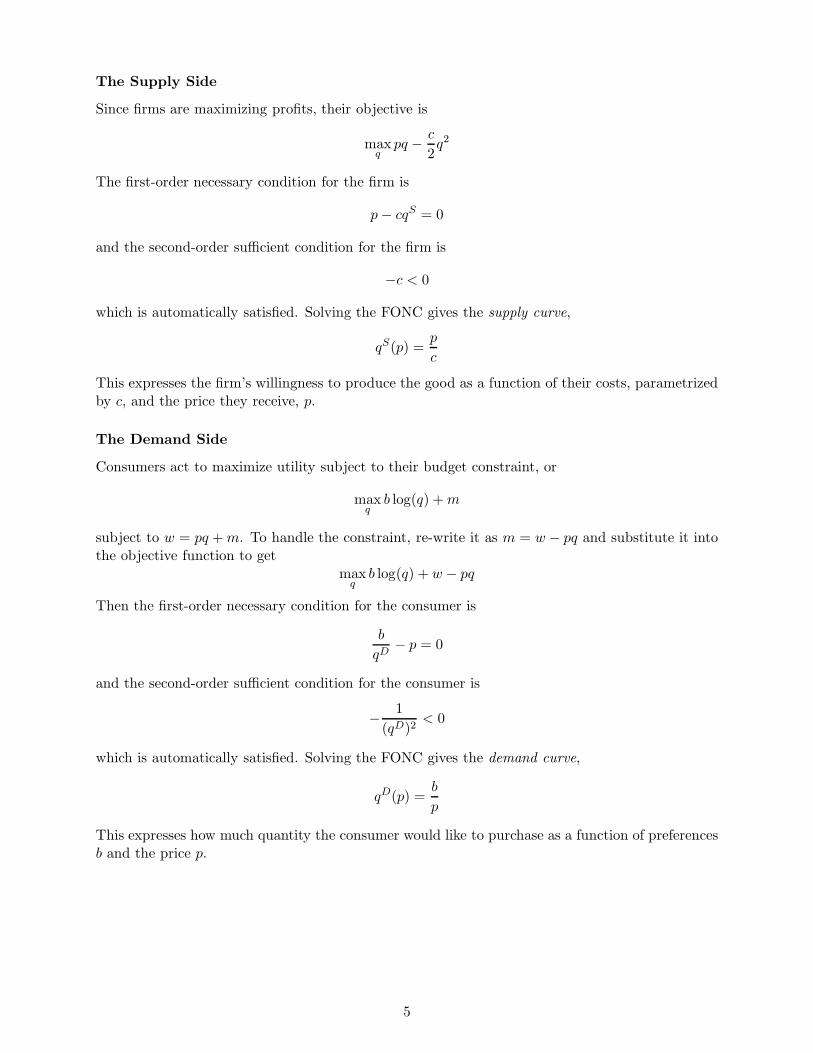
The Supply Side

Since firms are maximizing profits, their objective is

maxq

pq − c

2q2

The first-order necessary condition for the firm is

p− cqS = 0

and the second-order sufficient condition for the firm is

−c < 0

which is automatically satisfied. Solving the FONC gives the supply curve,

qS(p) =p

c

This expresses the firm’s willingness to produce the good as a function of their costs, parametrizedby c, and the price they receive, p.

The Demand Side

Consumers act to maximize utility subject to their budget constraint, or

maxq

b log(q) +m

subject to w = pq +m. To handle the constraint, re-write it as m = w − pq and substitute it intothe objective function to get

maxq

b log(q) + w − pq

Then the first-order necessary condition for the consumer is

b

qD− p = 0

and the second-order sufficient condition for the consumer is

− 1

(qD)2< 0

which is automatically satisfied. Solving the FONC gives the demand curve,

qD(p) =b

p

This expresses how much quantity the consumer would like to purchase as a function of preferencesb and the price p.

5

Market-Clearing Equilibrium

In equilibrium, supply equals demand, and the market-clearing price p∗ and market-clearing quan-tity q∗ are determined as

qD(p∗) = qS(p∗) = q∗

orb

p∗=

p∗

c= q∗

Solve for p∗ yieldsp∗ =

√bc

and

q∗ =

√b√c

Market Equilibrium

Notice that the variables of interest — p∗ and q∗ — are expressed completely in terms of theparameters of the model that are outside of any agents’ control, b and c. We can now vary b andc freely to see how the equilibrium price and quantity vary, and study how changes in tastes ortechnology will change behavior.

1.3 Basic questions of economic analysis

After building a model, two mathematical questions naturally arise,

• How do we know solutions exist to the agents’ maximization problems? (the Weierstasstheorem)

• How do we find solutions? (first order necessary conditions, second order sufficient conditions)

as well as two economic questions,

• How does an agent’s behavior respond to changes in the economic environment? (the implicitfunction theorem)

6

• How does an agent’s payoff respond to changes in the economic environment? (the envelopetheorem)

In Micro I, we learn in detail the nuts and bolts of solving agents’ problems in isolation (opti-mization theory). In Micro II, you learn — through general equilibrium and game theory — howto solve for the behavior when many agents are interacting at once (equilibrium and fixed-pointtheory).

The basic methodology for solving problems in Micro I is:

• Check that a solution exists to the problem using the Weierstrass theorem

• Build a candidate list of potential solutions using the appropriate first-order necessary con-ditions

• Find the global maximizer by comparing candidate solutions directly by computing theirpayoff, or use the appropriate second-order sufficient conditions to verify which are maxima

• Study how an agent’s behavior changes when economic circumstances change using the im-plicit function theorem

• Study how an agent’s payoffs changes when economic circumstances change using the envelopetheorem

Actually, the above is a little misleading. There are many versions of the Weierstrass theorem,the FONCs, the SOSCs, the IFT and the envelope theorem. The appropriate version depends onthe kind of problem you face: Is there a single choice variable or many? Are there equality orinequality constraints? And so on.

The entire class — including the parts of Mas-Colell-Whiston-Green that we cover — is nothingmore than the application of the above algorithm to specific problems. At the end of the course, itis imperative that you understand the above algorithm and know how to implement it to pass thecomprehensive exams.

We will start by studying the algorithm in detail for one-dimensional maximization problems inwhich agents only choose one variable. Then we will generalize it to multi-dimensional maximizationproblems in which agents choose many things at once.

Exercises

The exercises refer to the simple partial equilibrium model of Section 1.2.1. [Basics] As b and c change, how do the supply and demand curves shift? How do the

equilibrium price and quantity change? Sketch graphs as well as compute derivatives.

2. [Taxes] Suppose there is a tax t on the good q. A portion µ of t is paid by the consumerfor each unit purchased, and a portion 1 − µ of t is paid by the firm for each unit sold. How doesthe consumer’s demand function depend on µ? How does the firm’s supply function depend on µ?How does the equilibrium price and quantity p∗ and q∗ depend on µ? If t goes up, how are themarket clearing price and quantity affected? Sketch a graph of the equilibrium in this market.

3. [Long-run equilibrium] (i) Suppose that there are K firms in the industry with short-run cost

function C(q) =c

2q2, so that each firm produces q, but aggregate supply is Kq = Q. Consumers

maximize b log(Q) +m subject to w = pQ +m. Solve for the market-clearing price and quantityfor each K and the short-run profits of the firms. (ii) Suppose firms have to pay a fixed cost F toenter the industry. Find the equilibrium number of firms in the long run, K∗, if there is entry as

7

long as profits are strictly positive. How does K∗ vary in F , b and c? How do the market-clearingprice and quantity vary in the long run with F?

4. [Firm cost structure] Suppose a price-taking firm’s costs are C(q) = c(q)+F , where c(0) = 0,c′(0) > 0 and c′′(0) > 0 and F is a fixed cost. (i) Show that marginal cost C ′(q) intersects averagecost C(q)/q at the minimum of C(q)/q. This is the efficient scale. (ii) How does the firm’s optimalchoice of q depend on F?

5. [Monopoly] Suppose now that the consumers’ utility function is

2b√q +m

and the budget constraint is w = pq+m. Suppose there is a single firm with cost function C(q) = cq.(i) Derive the demand curve qD(p) and inverse demand curve pD(q). (ii) If the monopolist recognizesits influence on the market-clearing price and quantity, it will maximize

maxq

pD(q)q − cq

ormax

pqD(p)(p − c)

Show that the solutions to these problems are the same. If total revenue is pqD(p) show thatits derivative, the marginal revenue curve, lies below the total revenue curve, and compare themonopolist’s FONC with a price-taking firm’s FONC in the same market.

6. [Efficiency] A benevolent, utilitarian social planner (or well-meaning government) wouldchoose the market-clearing quantity to maximize the sum of the two agents’ payoffs, or

maxp,q

(v(q) + w − pq) + (pq −C(q))

Show that this outcome is the same as that selected by the perfectly competitive market. Concludethat a competitive equilibrium achieves the same outcome that a benevolent government would pick.Give an argument for why a government trying to intervene in a decentralized market would thenprobably achieve a worse outcome. Give an argument why a decentralized market would probablyachieve a worse outcome than a well-meaning government. Show that the allocation selected by thedecentralized market and utilitarian social planner is not the allocation selected by a monopolist.Sketch a graph of the situation.

Congratulations, you are now qualified to be a micro TA!

8

Chapter 2

Basic Math and Logic

These are basic definitions that appear in all of mathematics and modern economics, but reviewingit doesn’t hurt.

2.1 Set Theory

Definition 2.1.1 A set A is a collection of elements. If x is an element or member of A, thenx ∈ A. If x is not in A, then x /∈ A. If all the elements of A and B are the same, A = B. The setwith no elements is called the empty set, ∅.

We often enumerate sets by collecting the elements between braces, as

F = { Apples, Bananas, Pears }

F ′ = { Cowboys, Bears, Chargers, Colts}We can build up and break down sets as follows:

Definition 2.1.2 Let A,B and C be sets.

• A is a subset of B if all the elements of A are elements of B, written A ⊆ B; if there existsan element x ∈ A but x /∈ B, we can also write A ⊂ B.

• If A ⊆ B and B ⊆ A, then A = B.

• The set of all elements in either A or B is the union of A and B, written A ∪B.

• The set of all elements in both A and B is the intersection of A and B, written A ∩ B. IfA ∩B = ∅, then A and B are disjoint.

• Suppose A ⊂ B. The set of elements in B but not in A is the complement of A in B, writtenAc.

These precisely define all the normal set operations like union and intersection, and give exactmeaning to the symbol A = B. It’s easy to see that operations like union and intersection areassociative (check) and commutative (check). But how does taking the complement of a union orintersection behave?

Theorem 2.1.3 (DeMorgan’s Laws) For any sets A and B that are both subsets of X,

(A ∪B)c = Ac ∩Bc

9

and(A ∩B)c = Ac ∪Bc,

where the complement is taken with respect to X.

Proof Suppose x ∈ (A ∪ B)c. Then x is not in the union of A and B, so x is in neither A norB. Therefore, x must be in the complement of both A and B, so x ∈ Ac ∩ Bc. This shows that(A ∪B)c ⊂ Ac ∩Bc.

Suppose x ∈ Ac ∩ Bc. Then x is contained in the complement of both A and B, so it not amember of either set, so it is not a member of the union A ∪ B; that implies x ∈ (A ∪ B)c. Thisshows that (A ∪B)c ⊃ Ac ∩Bc.

If you ever find yourself confused by a complicated set relation ((A ∪ B ∩ C)c ∪D...), draw aVenn diagram and try writing in words what is going on.

We are interested in defining relationships between sets. The easiest example is a function,f : X → Y , which assigns a unique element of Y to at least some elements of X. However, ineconomics we will have to study some more exotic objects, so it pays to start slowly in definingfunctions, correspondences, and relations.

Definition 2.1.4 The (Cartesian) product of two non-empty sets X and Y is the set of all orderedpairs (x, y) = {x ∈ X, y ∈ Y }.

The product of two sets X and Y is often written X × Y . If it’s just one set copied over andover, X×X×...×X = Xn, and an ordered pair would be (x1, x2, ..., xn). For example R×R = R

2 isproduct of the real numbers with itself, which is just the plane. If we have a “set of sets”, {Xi}Ni=1,we often write ×N

i=1Xi or∏N

i=1 Xi.

Example Suppose two agents, A and B, are playing the following game: If A and B both choose“heads”, or HH, or both choose “tails”, or TT , agent B pays agent A a dollar. If one playerchooses tails and the other chooses heads, and vice versa, agent A pays agent B a dollar. ThenA and B both have the strategy sets SA = SB = {H,T}, and an outcome is an ordered pair(sA, sB) ∈ SA × SB. This game is called matching pennies.

Besides a Cartesian product, we can also take a space and investigate all of its subsets:

Definition 2.1.5 The power set of A is the set of all subsets of A, often written 2A, since it has2|A| members.

For example, take A = {a, b}. Then the power set of A is ∅, {a, b}, {a}, and {b}.

2.2 Functions and Correspondences

Definition 2.2.1 Let X and Y be sets. A function is a rule that assigns a single element y ∈ Y toeach element x ∈ X; this is written y = f(x) or f : X → Y . The set X is called the domain, and theset Y is called the range. Let A ⊂ X; then the image of A is the set f(A) = {y : x ∈ A, y = f(x)}.

Definition 2.2.2 A function f : X → Y is injective or one-to-one if for every x1, x2 ∈ X, x1 6= x2implies f(x1) 6= f(x2). A function f : X → Y is surjective or onto if for all y ∈ Y , there exists anx ∈ X such that f(x) = y.

Definition 2.2.3 A function is invertible if for every y ∈ Y , there is a unique x ∈ X for whichy = f(x).

10

Note that the definition of invertible is extremely precise: For every y ∈ Y , there is a uniquex ∈ X for which y = f(x).

Do not confuse whether or not a function is invertible with the following idea:

Definition 2.2.4 Let f : X → Y , and I ⊂ Y . Then the inverse image of I under f is the set ofall x ∈ X such that f(x) = y and y ∈ I.

Example On [0,∞), the function f(x) = x2 is invertible, since x =√y is the unique inverse

element. Then for any set I ⊂ [0,∞), the inverse image f−1(I) = {x :√y = x, y ∈ I}.

On [−1, 1], f(x) = x2 has the image set I = [0, 1]. For any y 6= 0, y ∈ I, we can solve forx = ±√

y, so that x2 is not invertible on [−1, 1]. However, the inverse image f−1([0, 1]) is [−1, 1],by the same reasoning.

There is an important generalization of a function called a correspondence:

Definition 2.2.5 Let X and Y be sets. A correspondence is a rule that assigns a subset F (x) ⊆ Yto each x ∈ X. Alternatively1, a correspondence is a rule that maps X into the power set of Y ,F : X → 2Y .

So a correspondence is just a “function with set-valued images”: The restriction on functionsthat f(x) = y and y is a singleton is being relaxed so that F (x) = Z where Z is a set containingelements of Y .

Example Consider the equation x2 = c. We can think of the correspondence X(c) as the set of(real) solutions to the equation. For c < 0, the equation cannot be solved, because x2 > 0, so X(c)is empty for c < 0. For c = 0, there is exactly one solution, X(c) = {0}, and X(c) happens to bea “function at that point”. But for c > 0, X(c) = {√c,−√

c}, since (−1)2 = 1: Here there is anon-trivial correspondence, where the image is a set with multiple elements.

Example Suppose two agents are playing “matching pennies”. Their payoffs can be succinctlyenumerated in a table:

B

H T

H 1,-1 -1,1

A T -1,1 1,-1

Suppose agent B uses a mixed strategy and plays randomly, so that σ = pr[Column uses H]. ThenA’s expected utility from using H is

σ1 + (1− σ)(−1)

while the row player’s expected utility from using T is

σ(−1) + (1− σ)(1)

We ask, “When is it an optimal strategy for the row player to use H against the column player’smixed strategy σ?”, or, “What is the row player’s best-response to σ?”

Well, H is strictly better than T if

σ1 + (1− σ)(−1) > σ(−1) + (1− σ)(1) → σ >1

2

1For reasons beyond our current purposes, there are advantages and disadvantages to each approach.

11

and H is strictly worse than T if

σ(−1) + (1 − σ)(1) > σ1 + (1− σ)(−1) → σ <1

2

But when σ = 1/2, the row player is exactly indifferent between H and T . Indeed, the row playercan himself randomize over any mix between H and T and get exactly the same payoff. Therefore,the row player’s best-response correspondence is

pr[Row uses H|σ] =

1 σ > 1/2

0 σ < 1/2

[0, 1] σ = 1/2

So correspondences arise naturally (and frequently!) in game theory.

Example Consider the maximization problem

maxx1,x2

x1 + x2

subject to the constraints x1, x2 ≥ 0, x1 + px2 ≤ 1.Since x1 and x2 are perfect substitutes, the solution is intuitively to pick the cheapest good and

buy only that one. However, in the case when p = 1, the objective and constraint lie on top of oneanother, and any pair x∗1 + x∗2 = 1 is a solution. The solution to the maximization problem then is

(x∗1(p), x∗2(p)) =

(0, 1/p) p < 1

(1, 0) p > 1

(z, 1 − z) p = 1, z ∈ [0, 1]

Therefore, we have a correspondence, where the optimal solution in the case when p = 1 is setvalued, [z, 1− z] for z ∈ [0, 1]. So correspondences arise naturally in optimization theory.

It turns out that correspondences are very common in microeconomics, even though they aren’tusually studied in calculus or undergraduate math courses.

2.3 Real Numbers and Absolute Value

The set of numbers we usually work in, (−∞,∞), is called the real numbers, or R. The symbols−∞ and ∞ are not in R (they are not even really numbers), but represent the idea of an unboundedprocess, like 1, 2, 3, .... The features of R that make it attractive follow from the intuitive idea thatR is a continuum, with no breaks. This is unlike the integers, Z = ...,−3,−2,−1, 0, 1, 2, 3, ..., whichhave spaces between each number.

Absolute value is given by

|x| =

−x if x < 0

0 if x = 0

x if x > 0

The most important feature of absolute value is that it satisfies

|x+ y| ≤ |x|+ |y|

And in particular,|x− y| ≤ |x|+ |y|

12

2.4 Logic and Methods of Proof

It really helps to get a sense of what is going on in this section, and return to it a few times over thecourse. Thinking logically and finding the most elegant (read as, “slick”) way to prove somethingis a skill that is developed. It is a talent, like composing or improvising music or athletic ability, inthat you begin with a certain stock of potential to which you can add by working hard and beingalert and careful when you see how other people do things. Even if you want to be an applied microor macro economist, you will someday need to make logical arguments that go beyond taking a fewderivatives or citing someone else’s work, and it will be easier if you remember the basic nuts andbolts of what it means to “prove” something.

Propositional Logic

Definition 2.4.1 A proposition is a statement that is either true or false.

For example, some propositions are

• “The number e is transcendental”

• “Every Nash equilibrium is Pareto optimal”

• “Minimum wage laws cause unemployment”

These statements are either true or false. If you think minimum wage laws sometimes causeunemployment, then you are simply asserting the third proposition is false, although a similarstatement that is more tentative might be true. The following are not propositions:

• “What time is it?”

• “This statement is false”

The first sentence is simply neither true nor false. The second sentence is such that if it were trueit would be false, and if it were false it would be true2. Consequently, you can arrange symbols inways that do not amount to propositions, so the definition is not meaningless.

Our goal in theory is usually to establish that “If P is true, then Q must be true”, or “P → Q”,or “ Q is a logical implication of P”. We begin with a set of conditions that take the form ofpropositions, and show that these propositions collectively imply the truth of another proposition.

Since any proposition P is either true or false, we can consider the proposition’s negation: Theproposition that is true whenever P is false, and false whenever P is true. We write the negation ofP in symbols as ¬P as “not P”. For example, “the number e is not transcendental”, “some Nashequilibria are not Pareto optimal”, and “minimum wage laws do not cause unemployment”. Notethat when negating a proposition, you have to take some care, but we’ll get to more on that later.

Consider the following variations on “P → Q”:

• The Converse: Q → P

• The Contrapositive: ¬Q → ¬P

• The Inverse: ¬P → ¬Q2Note that this sentence is not a proposition not because it “contradicts” the definition of a proposition, but

because it fails to satisfy the definition.

13

The converse is usually false, but sometimes true. For example, a differentiable function iscontinuous (“differentiable → continuous” is true), but there are continuous functions that arenot differentiable (“continuous → differentiable” is false). The inverse, likewise, is usually false,since non-differentiable functions need not be discontinuous, since many functions with kinks arecontinuous but non-differentiable, like |x|. The contrapositive, however, is always true if P → Qis true, and always false if P → Q is false. For example, “a discontinuous function cannot bedifferentiable” is a true statement. Another way of saying this is that a claim P → Q and itscontrapositive have the same truth value (true or false). Indeed, it is often easier to prove thecontrapositive than to prove the original claim.

While the above paragraph shows that the converse and inverse need not be true if the originalclaim P → Q is true, we should show more concretely that the contrapositive is true. Why is this?Well, if P → Q, then whenever P is true, Q must be true also, which we can represent in a table:

P Q P → Q

T T T

T F F

F T T

F F T

So the first two columns say what happens when P and Q are true or false. If P and Q are bothtrue, then of course P → Q is true. But if P and Q are both false, then of course P → Q is alsoa true statement. The proposition “P → Q” is actually only false when P is true but Q is false,which is the second line. Now, as for the contrapositive, the truth table is:

P Q ¬Q → ¬PT T T

T F F

F T T

F F T

By the same kind of reasoning, when P and Q are both true or both false, ¬Q → ¬P is true. In thecase where P is true but Q is false, we have ¬Q implies ¬P , but P is true, so ¬Q → ¬P is false.Thus, we end up with exactly the same truth values for the contrapositive as for the original claim,so they are equivalent. To see whether you understand this, make a truth table for the inverse andconverse, and compare them to the truth table for the original claim.

Quantifiers and negation

Once you begin manipulating the notation and ideas, you must inevitably negate a statement like,“All bears are brown.” This proposition has a quantifier in it, namely the word “all”. In thissituation, we want to assert that “All bears are brown” is false; there are, after all, giant pandasthat are black and white and not brown at all. So the right negation is something like, “Some bearsare not brown”. But how do we get “some” from “all” and “not brown” from “brown” in moregeneral situations without making mistakes?

Definition 2.4.2 Given a set A, the set of elements S that share some property P is writtenS = {x ∈ A : P (x)} (e.g., S1 = {x ∈ R : 2x > 4} = {x ∈ R : x ≥ 2}) .

Definition 2.4.3 In a set A, if all the elements x share some property P , ∀x ∈ A : P (x). If thereexists an element x ∈ A that satisfies a property P , then write ∃x ∈ A : P (x). The symbol ∀ is theuniversal quantifier and the symbol ∃ is the existential quantifier.

So a claim might be made,

14

• All allocations of goods in a competitive equilibria of an economy are Pareto optimal.

Then we are implicitly saying: Let A be the set of all allocations generated by a competitiveequilibrium, and let P (a) denote the claim that a is a “Pareto optimal allocation”, whatever thatis. Then we might say, “If a ∈ A, P (a)”, or

• ∀a ∈ A : P (a)

Negating propositions with quantifiers can be very tricky. For example, consider the claim:“Everybody loves somebody sometime.” We have three quantifiers, and it is unclear what orderthey should go in. The negation of this statement becomes a non-trivial problem precisely becauseof how many quantifiers are involved: Should the negation be, “Everyone hates someone sometime?”Or “Someone hates everyone all the time”? It requires care to get these details right. Recall thedefinition of negation:

Definition 2.4.4 Given a statement P (x), the negation of P (x) asserts that P (x) is false for x.The negation of a statement P (x) is written ¬P (x).

The rules for negating statements are

¬(∀x ∈ A : P (x)) = ∃x ∈ A : ¬P (x)

and¬(∃x ∈ A : P (x)) = ∀x ∈ A : ¬P (x)

For example, the claim “All allocations of goods in a competitive equilibria of an economy arePareto optimal” could be written in the above form as follows: Let A be the set of allocationsachievable in a competitive equilibrium of an economy (whatever that is), let a ∈ A be a particularallocation, and let P (a) be the proposition that the allocation is Pareto optimal (whatever that is).Then the claim is equivalent to the statement ∀a ∈ A : P (a). Then the negation of that statement,then, is

• ∃a ∈ A : ¬P (a)

or in words, “There exists an allocation of goods in some competitive equilibrium of an economythat is not Pareto optimal.”

Be careful about “or” statements. In proposition logic, P → Q1 or Q2 means, “P logicallyimplies Q1, or Q2, or both”. So the negation of “or” statements is that “P implies either not Q1 ornot Q2 or neither”. For example, “All U.S. Presidents were U.S. citizens and older than 35 whenthey took office” is negated to “There’s no U.S. President who wasn’t a U.S. citizen, or youngerthan 35, or both, when they took office.”

Some examples:

• “A given strategy profile is a Nash equilibrium if there is no player with a profitable deviation.”Negating this statement gives, “A given strategy profile is not a Nash equilibrium if thereexists a player with a profitable deviation.”

• “A given allocation is Pareto efficient if there is no agent who can be made strictly betteroff without making some other agent worse off.” Negating this statement gives, “A givenallocation is not Pareto efficient if there exists an agent who can be made strictly better offwithout making any other agent worse off.”

• “A continuous function with a closed, bounded subset of Euclidean space as its domain alwaysachieves its maximum.” Negating this statement gives, “A function that is not continuousor whose domain is not a closed, bounded subset of Euclidean space may not achieve amaximum.”

Obviously, we are not logicians, so our relatively loose statements of ideas will have to be negatedwith some care.

15

2.4.1 Examples of Proofs

Most proofs use one of the following approaches:

• Direct proof: Show that P logically implies Q

• Proof by Contrapositive: Show that ¬Q logically implies ¬P

• Proof by Contradiction: Assume P and ¬Q, and show this leads to a logical contradiction

• Proof by Induction: Suppose we want to show that for any natural number n = 1, 2, 3, ...,P (n) → Q(n). A proof by induction shows that P (1) → Q(1) (the base case), and that forany n, if P (n) → Q(n) (the induction hypothesis), then P (n+1) → Q(n+1). Consequently,P (n) → Q(n) is true for all n.

• “Disproof by Counterexample”: Let ∀x ∈ A : P (x) be a statement we wish to disprove. Showthat ∃x′ ∈ A such that P (x′) is false.

The claim might be fairly complicated, like

• If “f(x) is a bounded, increasing function on [a, b]”, then “the set of points of discontinuityof f() is a countable set”.

The “P” is, (f(x) is a bounded, increasing function on [a, b]), and the “Q” is (the set of points ofdiscontinuity of f(x) is a countable set). To prove this, we could start by using P to show Q mustbe true. Or, in a proof by contrapositive, we could prove that if the function has an uncountablenumber of discontinuities on [a, b], then f(x) is either unbounded, or decreasing, or both. Or, ina proof by contradiction, we could assume that the function is bounded and increasing, but thatthe function has an uncountable number of discontinuities. The challenge for us is to make surethat while we are using mathematical sentences and definitions, no logical mistakes are made inour arguments.

Each method of proof has its own advantages and disadvantages, so we’ll do an example of eachkind now.

A Proof by Contradiction

Theorem 2.4.5 There is no largest prime.

Proof Suppose there was a largest prime number, n. Let p = n ∗ (n− 1) ∗ ... ∗ 1+1. Then p is notdivisible by any of the first n numbers, so it is prime and greater than n, since n∗(n−1)∗ ..∗1+1 >n ∗ 1+1 > n. So p is a prime number larger than n — this is a contradiction, since n was assumedto be the largest prime. Therefore, there is no largest prime.

A Proof by Contrapositive

Suppose we have two disjoint sets, M and W with |M | = |W |, and are looking for a matching ofelements in M to elements in W — a relation mapping each element from M into W and vice versa,which is one-to-one and onto. Each element has a “quality” attached, either qm ≥ 0 or qw ≥ 0, andthe value of the match is v(qm, qw) =

12qmqw. The assortative match is the one where the highest

quality agents are matched, the second-highest quality agents are matched, and so on. If agent mand agent w are matched, then h(m,w) = 1; otherwise h(m,w) = 0.

Theorem 2.4.6 If a matching maximizes∑

m

∑

w h(m,w)v(qm, qw), then it is assortative.

16

Proof Since the proof is by contrapositive, we need to show that any matching that is not assorta-tive does not maximize

∑

m

∑

w hmwv(qm, qw) — i.e., any non-assortative match can be improved.If the match is not assortative, we can find two sets of agents where qm1 > qm2 and qw1 > qw2 ,

but h(m1, w2) = 1 and h(m2, q1) = 1. Then the value of those two matches is

qm1qw2 + qm2qw1

If we swapped the partners, the value would be

qm1qw1 + qm2qw2

and{qm1qw1 + qm2qw2} − {qm1qw2 + qm2qw1} = (qm1 − qm2)(qw1 − qw2) > 0

So a non-assortative match does not maximize∑

m

∑

w h(m,w)v(qm, qw). .

What’s the difference between proof by contradiction and proof by contrapositive? In proof bycontradiction, you get to use P and ¬Q to arrive at a contradiction, while in proof by contrapositive,you use ¬Q to show that ¬P is a logical implication, without using P or ¬P in the proof.

A Proof by Induction

Theorem 2.4.7∑n

i=1 i =1

2n(n+ 1)

Proof Basis Step: Let n = 1. Then∑1

i=1 i = 1 =1

21(1+1) = 1. So the theorem is true for n = 1.

Induction Step: Suppose∑n

i=1 i =1

2n(n+1); we’ll show that

∑n+1i=1 i =

1

2(n+1)(n+2). Now

add n+ 1 to both sides:n∑

i=1

i+ (n+ 1) =1

2n(n+ 1) + (n+ 1)

Factoring1

2(n+ 1) out of both terms gives

n+1∑

i=1

i =1

2(n+ 1)(n + 2)

And the induction step is shown to be true.Now, since the basis step is true (P (1) → Q(1) is true), and the induction step is true (“P (n) →

Q(n)” → “P (n + 1) → Q(n+ 1)”), the theorem is true for all n.

Disproof by Counter-example

Definition 2.4.8 Given a (possibly false) statement ∀x ∈ A : P (x), a counter-example is anelement x′ of A for which ¬P (x′).

For example, “All continuous functions are differentiable.” This sounds like it could be true.Continuous functions have no jumps and are pretty well-behaved. But it’s false. The negation ofthe statement is, “There exist continuous functions that are not differentiable.” Maybe we canprove that?

17

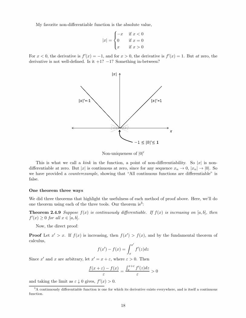
My favorite non-differentiable function is the absolute value,

|x| =

−x if x < 0

0 if x = 0

x if x > 0

For x < 0, the derivative is f ′(x) = −1, and for x > 0, the derivative is f ′(x) = 1. But at zero, thederivative is not well-defined. Is it +1? −1? Something in-between?

Non-uniqueness of |0|′

This is what we call a kink in the function, a point of non-differentiability. So |x| is non-differentiable at zero. But |x| is continuous at zero, since for any sequence xn → 0, |xn| → |0|. Sowe have provided a counterexample, showing that “All continuous functions are differentiable” isfalse.

One theorem three ways

We did three theorems that highlight the usefulness of each method of proof above. Here, we’ll doone theorem using each of the three tools. Our theorem is3:

Theorem 2.4.9 Suppose f(x) is continuously differentiable. If f(x) is increasing on [a, b], thenf ′(x) ≥ 0 for all x ∈ [a, b].

Now, the direct proof:

Proof Let x′ > x. If f(x) is increasing, then f(x′) > f(x), and by the fundamental theorem ofcalculus,

f(x′)− f(x) =

∫ x′

xf ′(z)dz

Since x′ and x are arbitrary, let x′ = x+ ε, where ε > 0. Then

f(x+ ε)− f(x)

ε=

∫ x+εx f ′(z)dz

ε> 0

and taking the limit as ε ↓ 0 gives, f ′(x) > 0.

3A continuously differentiable function is one for which its derivative exists everywhere, and is itself a continuousfunction.

18

In this proof, we use the premise to prove the conclusion directly, without using the conclusion.Let’s try a proof by contrapositive.

Proof This proof is by contrapositive, so we will show that if f ′(x) < 0 for all x ∈ [a, b], then f(x)is decreasing.

Suppose f ′(x) < 0 for all x ∈ [a, b], and x′ > x are in [a, b]. Then

f(x′)− f(x) =

∫ x′

xf ′(z)dz < 0

so that f(x′) < f(x), as was to be shown.

Here, instead of showing that an increasing function has positive derivatives, we showed thatnegative derivatives implied a decreasing function. In some sense, the proof was easier, even thoughthe approach involved more thought. The last proof is by contradiction:

Proof This proof is by contradiction, so we assume that for all x′ > x in [a, b], f(x′) > f(x), butf ′(x) < 0 for all x ∈ [a, b].

If x′ > x, then f(x′) − f(x) =∫ x′

x f ′(z)dz < 0, so that f(x′) < f(x). But we assumed thatf(x′) > f(x), so we are lead to a contradiction.

See how we get to use both 6 P and Q to arrive at a contradiction? That is the key advantage.The disadvantage is that you can often learn more from a direct proof about the mathematicalsituation than you can from a proof by contradiction, since the first often constructs the objects ofinterest or shows how various conditions give rise to certain properties.

Necessary and Sufficient Conditions

If P → Q and Q → P , then we often say “P if and only if Q”, or “P is necessary for Q and Q issufficient for P”.

Consider

• To be a lawyer, it is necessary to have attended law school.

• To be a lawyer, it is sufficient to have passed the bar exam.

To pass the bar exam, it is required that a candidate have a law degree. On the other hand, alaw degree alone does not entitle someone to be a lawyer, since they still need to be certified. So alaw degree is a necessary condition to be a lawyer, but not sufficient. On the other hand, if someonehas passed the bar exam, they are allowed to represent clients, so it is a sufficient condition to bea lawyer. There is clearly a gap between the necessary condition of attending law school, and thesufficient condition of passing the bar exam; namely, passing the bar exam.

Let’s look at a more mathematical example:

• A necessary condition for a point x∗ to be a local maximum of a differentiable function f(x)on (a, b) is that f ′(x∗) = 0.

• A sufficient condition for a point x∗ to be a local maximum of a differentiable function f(x)on (a, b) is that f ′(x∗) = 0 and f ′′(x∗) < 0.

Why is the first condition necessary? Well, if f(x) is differentiable on (a, b) and f ′(x∗) > 0, wecan take a small step to x∗ + h and increase the value of the function (alternatively, if f ′(x∗) < 0,take a small step to x∗ − h and you can also increase the value of the function). Consequently, x∗

could not have been a local maximum. So it is necessary that f ′(x∗) = 0.

19

Why is the second condition sufficient? Well, Taylor’s theorem says that

f(x) = f(x∗) + f ′(x∗)(x− x∗) + f ′′(x∗)(x∗ − x)2

2+ o((h)3)

where x∗ − x = h and o(h3) goes to zero as h goes to zero faster than the (x∗ − x)2 and (x∗ − x)terms. Since f ′(x∗) = 0, we then have

f(x) = f(x∗) + f ′′(x∗)(x− x∗)2

2+ o(h3)

so that for x sufficiently close to x∗,

f(x∗)− f(x) = −f ′′(x∗)(x∗ − x)2

2

so that f(x∗) > f(x) only if f ′′(x∗) < 0. So if the first-order necessary conditions and second-order sufficient conditions are satisfied, x∗ must be a solution. However, there is a substantial gapbetween the first-order necessary and second-order sufficient conditions.

For example, consider f(x) = x3 on (−1, 1). The point x∗ = 0 is clearly a solution of thefirst-order necessary conditions, and f ′′(0) = 0 as well. However, f(1/2) = (1/2)3 > 0 = f(0),so the point x∗ is a critical point, but not a maximum. Similarly, suppose we try to maximizef(x) = x2 on (−1, 1). Again, x∗ = 0 is a solution to the first-order necessary conditions, but it isa minimum, not a maximum. So the first-order necessary conditions only identify critical points,but these critical points come in three flavors: maximum, minimum, and saddle-point.

Alternatively, consider the function

g(x) =

x ,−∞ < x < 5

5 , 5 ≤ x ≤ 10

10− x , 10 < x < ∞

This function looks like a plateau, where the set [5, 10] all sits at a level of 5, and everything beforeand after drops off. The necessary conditions are satisfied for all x strictly between 5 and 10,since f ′(x) = 0 for x strictly between 5 and 10. But the sufficient conditions aren’t satisfied, sincef ′′(x) = 0 for x strictly between 5 and 10. These points are all clearly global maxima, but thesecond-order sufficient conditions require strict negativity to rule out pathologies like f(x) = x3.

So, even when you have useful necessary and sufficient conditions, there can be subtle gaps thatyou miss if you’re not careful.

Exercises

1. If A and B are sets, prove that A ⊆ B iff A ∩B = A.2. Prove the distributive law

A ∩ (B ∩ C) = (A ∩B) ∩ (A ∩ C)

and the associative law(A ∪B) ∪ C = A ∪ (B ∪ C)

What is ((A ∪B)∪))c?3. Sketch graphs of the following sets:

{(x, y) ∈ R2 : x ≥ y}

20

{(x, y) ∈ R2 : x2 + y2 ≤ 1}

{(x, y) ∈ R2 :

√xy ≥ 5}

{(x, y) ∈ R2 : min{x, y} ≥ 5}

4. Write the converse and contrapositive of the following statements (note that you don’t haveto know what any of the statements actually mean to negate them) :

• A set X is convex if, for every x1, x2 ∈ X and λ ∈ [0, 1], the element xλ = λx1 + (1− λ)x2 isin X.

• The point x∗ is a maximum of a function f on the set A if there exists no x′ ∈ A such thatf(x′) > f(x).

• A strategy profile is a subgame perfect Nash equilibrium if, for every player and in everysubgame, the strategy profile is a Nash equilibrium.

• A function is uniformly continuous on a set A if, for all ε > 0 there exists a δ > 0 such thatfor all x, c ∈ A, |x− c| < δ, |f(x)− f(c)| < ε.

• Any competitive equilibrium (x∗, y∗, p∗) is a Pareto optimal allocation.

21

Part I

Optimization and ComparativeStatics in R

22

Chapter 3

Basics of R

Deliberate behavior is central to every microeconomics model, since we assume that agents act toget the best payoff possible available to them, given the behavior of other agents and exogenouscircumstances that are outside their control.

Some examples are:

• A firm hires capital K and labor L at prices r and w per unit, respectively, and has productiontechnology function F (K,L). It receives a price p per unit it sells of its good. It would liketo maximize profits,

π(K,L) = pF (K,L) − rK − wL

• A consumer has utility function u(x) over bundles of goods x = (x1, x2, ..., xN ), and a budgetconstraint w ≤ ∑N

i=1 pixi. The consumer wants to maximize utility, subject to his budgetconstraint:

maxx

u(x)

subject to∑

i pixi ≤ w.

• A buyer goes to a first-price auction, where the highest bidder wins the good and pays hisbid. His value for the good is v, and the probability he wins, conditional on his bid, is p(b).If he wins, he gets a payoff v − b, while if he loses, he gets nothing. Then he is trying tomaximize

maxb

p(b)(v − b) + (1− p(b))0

These are probably very familiar to you. But, there are other, related problems of interest youmight not have thought of:

• A firm hires capital K and labor L at prices r and w per unit, respectively, and has productiontechnology function F (K,L). It would like to minimize costs, subject to producing q units ofoutput, or

minK,L

rK +wL

subject to F (K,L) = q.

• A consumer has utility function u(x) over bundles of goods x = (x1, x2, ..., xN ), and a budgetconstraint w ≤ ∑N

i=1 pixi. The consumer would like to minimize the amount they spend,subject to achieving utility equal to u, or

minx

N∑

i=1

pixi

subject to u(x) ≥ u.

23

• A seller faces N buyers, each of whom has a value for the good unobservable to the seller. Howmuch revenue can the seller raise from the transaction, among all possible ways of solicitinginformation from the buyers?

We want to develop some basic, useful facts about solving these kinds of models. There arethree questions we want to answer:

• When do solutions exist to maximization problems? (The Weierstrass theorem)

• How do we find candidate solutions? (First-order necessary conditions)

• How do we show that a candidate solution is a maximum? (Second-order sufficient conditions)

Since we’re going to study dozens of different maximization problems, we need a general wayof expressing the idea of a maximization problem efficiently:

Definition 3.0.10 A maximization problem is a payoff function or objective function, f(x, t),and a choice set or feasible set, X. The agent is then trying to solve

maxx∈X

f(x, t)

The variable x is a choice variable or control, since the agent gets to decide its value. The variablet is an exogenous variable or parameter, over which the agent has no control.

For this chapter, agents can choose any real number: Firms pick a price, consumers pick aquantity, and so on. This means that X is the set of real numbers, R. Also, unless we areinterested in t in particular, we often ignore the exogenous variables in an agent’s decision problem.For example, we might write π(q) = pq − cq2, even though π() depends on p and c.

A good question to start with is, “When does a maximizer of f(x) exist?” While this questionis simple to state in words, it is actually pretty complicated to state and show precisely, which iswhy this chapter is fairly “math-heavy”.

3.0.2 Maximization and Minimization

A function is a mapping from some set D, the domain, uniquely into R = (−∞,∞), the realnumbers, and we write f : D → R. For example,

√x : [0,∞) → R. The image of D under f(x) is

the set f(D). For example,√D = [0,∞), and for log(x) : (0,∞) → R, we have log(D) = (−∞,∞).

It turns out that the properties of the domain D and the function f(x) both matter for us.

Definition 3.0.11 A point x∗ is a global maximizer of f : D → R if, for any other x′ in D,

f(x∗) ≥ f(x′)

A point x∗ is a local maximizer of f : D → R if, for some δ > 0 and for any other x′ in(x∗ − δ, x∗ + δ) ∩D,

f(x∗) ≥ f(x′)

24

Domain, Image, Maxima, Minima

So a local maximum is basically saying, “If we restrict attention to (x∗ − δ, x∗ + δ) instead of(a, b), then x∗ is a global maximum in (x∗ − δ, x∗ + δ).” In even less mathematical terms, “x∗ is alocal maximum if it does at least as well as anything nearby.”

A point f(x∗) is a local or global minimum if, instead of f(x∗) ≥ f(x′) above, we have f(x∗) ≤f(x′). However, we can focus on just maximization or just minimization, since

Theorem 3.0.12 If x∗ is a local maximum of f(), then x∗ is a local minimum of −f().

Proof If f(x∗) ≥ f(x′) for all x′ in (x∗ − δ, x∗ + δ) for some δ > 0, then −f(x∗) ≤ −f(x′) for allx′ in (x∗ − δ, x∗ + δ), so it is a local minimum.

So whenever you have a minimization problem,

minx

f(x)

you can turn it into a maximization problem

maxx

−f(x)

and forget about minimization entirely.

25

Maximization vs. Minimization

On the other hand, since I have programmed myself to do this automatically, I find it annoyingwhen a book is written entirely in terms of minimization, and some of the rules used down theroad for minimization (second-order sufficient conditions for constrained optimization problems)are slightly different than those for maximization.

3.1 Existence of Maxima/Maximizers

So what do we mean by “existence of a maximum or maximizer”?Before moving to functions, let’s start with the maximum and minimum of a set. For a set

F = [a, b] with a and b finite, the maximum is b and the minimum is a — these are members ofthe set, and b ≥ x for all other x in S, and a ≤ x for all other x in S.

If we consider the set E = (a, b) however, the points b and a are not actually members of theset, although b ≥ x for all x in E, and a ≤ x for all x in E. We call b the least upper bound of E,or the supremum,

sup(a, b) = b

and a is the greatest lower bound of E, or the infimum,

inf(a, b) = a

Even if the maximum and minimum of a set don’t exist, the supremum and infimum always do(though they may be infinite, like for (a,∞)).

Since function is a rule that assigns a real number to each x in the domain D, the image of Dunder f is going to be a set, f(D). For maximization purposes, we are interested in whether theimage of a function includes its largest point or not.

For example, the function f(x) = x2 on [0, 1] achieves a maximum at x∗ = 1, since f(1) =1 > f(x) for 0 ≤ x < 1, and sup f([0, 1]) = max f([0, 1]). However, if we consider f(x) = x2 on(0, 1), the supremum of f(x) is still 1, since 1 is the least upper bound of f((0, 1)) = (0, 1), but thefunction does not achieve a maximum.

26

Existence and Non-existence

Why? On the left, the graph has no “holes”, so it moves smoothly to the highest point. Onthe right, however, a point is “missing” from the graph exactly where it would have achieved itsmaximum. This is the difference between a maximizer (left) and a supremum when a maximizerfails to exist (right). Why does this happen? In short, because the choice set on the left, [a, b],“includes all its points”, while the choice set on the right, (a, b), is missing a and b.

To be a bit more formal, suppose x′ ∈ (0, 1) is the maximum of f(x) = x2 on (0, 1). It mustbe less than 1, since 1 is not an element of the choice set. Let x′′ = (1 − x′)/2 + x′ — this is thepoint exactly halfway between x′ and 1. Then f(x′′) > f(x′), since f(x) is increasing. But then x′

couldn’t have been a maximizer. This is true for all x′ in (0, 1), so we’re forced to conclude thatno maximum exists.

But this isn’t the only way something can go wrong. Consider the function on [0, 1] where

g(x) =

x 0 ≤ x ≤ 1

2

2− x1

2< x ≤ 1

Again, the function’s graph is missing a point precisely where it would have achieved a maximum,at 1/2. Instead, it takes the value 1/2 instead of 3/2.

27

So in either case, the function can fail to achieve a maximum. In one situation, it happensbecause the domainD has the wrong features: It is missing some key points. In the second situation,it happens because the function f has the wrong features: It jumps around in unfortunate ways.

Consequently, the question is: What features of the domain D and the function f(x) guaranteethat supx∈D f(x) = m∗ is equal to f(x∗) for some x ∈ D?

Definition 3.1.1 A (global) maximizer of f(x), x∗, exists if f(x∗) = sup f(x), and f(x∗) is the(global) maximum of f().

3.2 Intervals and Sequences

Intervals are special subsets of the real numbers, but some of their properties are key for optimiza-tion theory.

Definition 3.2.1 The set (a, b) = {x : a < x < b} is open, while the set [a, b] = {x : a ≤ x ≤ b} isclosed. If −∞ < a < b < ∞, the sets (a, b) and [a, b] are bounded (both the endpoints a and b arefinite).

A sequence xn = x1, x2, ... is a rule that assigns a real number to each of the natural (counting)numbers, N = 1, 2, 3, ....

Some basic sequences are:

• Let xn = n. Then the sequence is 1, 2, 3, ...

• Let xn =1

n. Then the sequence is 1,

1

2,1

3, ...

• Let xn = (−1)n−1 1

n. Then the sequence is 1,−1

2,1

3,−1

4...

• Let x1 = 1, x2 = 1, and for n > 2, xn = xn−1+xn−2. Then the sequence is 1, 1, 2, 3, 5, 8, 13, 21, ...

• Let xn = sin(nπ

2

)

. Then the sequence is 1, 0,−1, 0, ...

At first, they might seem like a weird object to study when our goal is to understand functions.A function is basically an uncountable number of points, while sequences are countable, so it seemslike we would lose information by simplifying an object this way. However, it turns out thatstudying how functions f(x) act on a sequence xn gives us all the information we need to studythe behavior of a function, without the hassle of dealing with the function itself.

Definition 3.2.2 A sequence xn = x1, x2, .... is a function from N → R. A sequence converges tox if, for all ε > 0 there exists an N such that n > N implies |xn − x| < ε. Then we write

limn→∞

xn = x

and x is the limit of xn.

Everyone’s favorite convergent sequence is

xn =1

n= 1,

1

2,1

3, ...

and the limit of xn is zero. Why? First, for any positive number ε, I can make |xn − 0| < ε bypicking n large enough. Just take n > N = 1/ε, so that

1

n<

1

1/ε= ε

28

Second, since ε was arbitrary, it might as well be zero. Therefore, xn → 0 as n → ∞. Notice,however, how 1/n is never actually equal to zero for finite n; it is only in the limit that it hits itslower bound. This is another example of the difference between minimum and infimum: inf xn = 0but minxn does not exist, since 1/n > 0 for all n.

Everyone’s favorite non-convergent or divergent sequence is

xn = n

Pick any finite number ε, and I can make |xn| > ε, contrary to the definition of convergence. How?Just make |n| > ε. This sequence goes off to infinity, and its long-run behavior doesn’t “settledown” to any particular number.

Definition 3.2.3 A sequence xn is bounded if |xn| ≤ M for some finite real number M .

But boundedness alone doesn’t guarantee that a sequence converges, and just because a sequencefails to converge doesn’t mean that it’s not interesting. Consider

xn = cos

((n− 1)π

2

)

= 1, 0,−1, 0, 1, 0,−1, ...

This function fails to converge (right?). But it’s still quite well-behaved. Every even term is zero,

x2k = 0, 0, 0

and it includes a convergent string of ones,

x4(k−1)+1 = 1, 1, 1, ...

and a convergent string of −1’s,

x4(k−1)+3 = −1,−1,−1, ...

So the sequence xn — even though it is non-convergent — is composed of three convergent se-quences. These building blocks are important enough to deserve a name:

Definition 3.2.4 Let nk be a sequence of natural numbers, with n1 < n2 < ... < nk < .... Thenxnk

is a sub-sequence of xn.

It turns out that every bounded sequence has at least one sub-sequence that is convergent.

Theorem 3.2.5 (Bolzano-Weierstrass Theorem) Every bounded sequence has a convergentsubsequence.

This seems like an esoteric (and potentially useless) result, but it is actually a fundamental toolin analysis. Many times, we have a sequence of interest but know very little about it. To study itsbehavior, we use the Bolzano-Weierstrass to find a convergent sub-sequence, and sometimes that’senough.

29

3.3 Continuity

In short, a function is continuous if you can trace its graph without lifting your pencil off the paper.This definition is not precise enough to use, but it captures the basic idea: The function has no“jumps” where the value f(x) is changing very quickly even though x is changing very little. Thereason continuity is so important is because continuous functions preserve properties of sets likebeing open, closed, or bounded. For example, if you take a set S = (a, b) and apply a continuousfunction f() to it, the image f(S) is an open interval (c, d). This is not the case for every function.

The most basic definition of continuity is

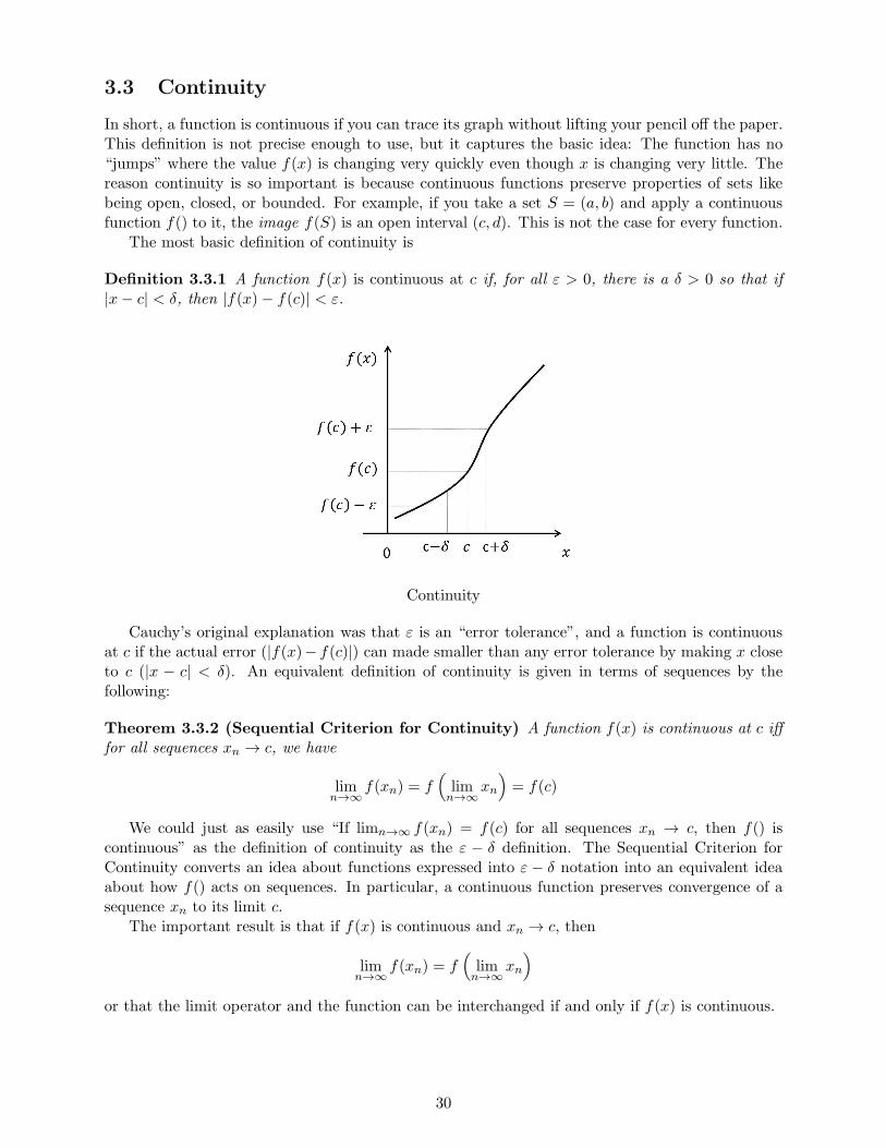
Definition 3.3.1 A function f(x) is continuous at c if, for all ε > 0, there is a δ > 0 so that if|x− c| < δ, then |f(x)− f(c)| < ε.

Continuity

Cauchy’s original explanation was that ε is an “error tolerance”, and a function is continuousat c if the actual error (|f(x)− f(c)|) can made smaller than any error tolerance by making x closeto c (|x − c| < δ). An equivalent definition of continuity is given in terms of sequences by thefollowing:

Theorem 3.3.2 (Sequential Criterion for Continuity) A function f(x) is continuous at c ifffor all sequences xn → c, we have

limn→∞

f(xn) = f(

limn→∞

xn

)

= f(c)

We could just as easily use “If limn→∞ f(xn) = f(c) for all sequences xn → c, then f() iscontinuous” as the definition of continuity as the ε − δ definition. The Sequential Criterion forContinuity converts an idea about functions expressed into ε − δ notation into an equivalent ideaabout how f() acts on sequences. In particular, a continuous function preserves convergence of asequence xn to its limit c.

The important result is that if f(x) is continuous and xn → c, then

limn→∞

f(xn) = f(

limn→∞

xn

)

or that the limit operator and the function can be interchanged if and only if f(x) is continuous.

30

3.4 The Extreme Value Theorem

Up to this point, what are the facts that you should internalize?

• Sequences are convergent only if they settle down to a constant value in the long run

• Every bounded sequence has a convergent subsequence, even if the original sequence doesn’tconverge (Bolzano-Weierstrass Theorem)

• A function is continuous if and only if limn→∞ f(xn) = f(x) for all sequences xn → x

With these facts, we can prove theWeierstrass Theorem, also called the Extreme Value Theorem.

Theorem 3.4.1 (Weierstrass’ Extreme Value Theorem) If f : [a, b] → R is a continuousfunction and a and b are finite, then f achieves a global maximum on [a, b].

First, let’s check that if any of the assumptions are violated, then examples exist where f doesnot achieve a maximum. Recall our examples of functions that failed to achieve maxima, f(x) = x2

on (0, 1) and

g(x) =

x 0 ≤ x ≤ 1

2

2− x1

2< x ≤ 1

on [0, 1]. In the first example, f(x) is continuous, but the set (0, 1) is open, unlike [a, b], violating thehypotheses of the Weierstrass theorem. In the second example, the function’s domain is closed andbounded, but the function is discontinuous, violating the hypotheses of the Weierstrass theorem.

So the reason the Weierstrass theorem is useful is that it provides sufficient conditions for afunction to achieve a maximum, so that we know for sure, without exception, that any continuousf(x) on a closed, bounded set [a, b] will achieve a maximum.

Proof Suppose thatsup f(x) = m∗

We know m∗ < ∞, since if f(x) is continuous on [a, b], it is well-defined for its whole domain andhas no asymptotes (unlike 1/x on [0, 1], which is discontinuous at zero). We want to show thatthere exists an x∗ in [a, b] so that f(x∗) = m∗.

Step 1: Since m∗ is the supremum of f(), we can find a sequence of points {xn} = x1, x2, ... in[a, b] so that

m∗ − 1

n≤ f(xn) ≤ m∗

Why? We show this by contradiction. If the above inequality was violated, then for some n, we

would not be able to find an xn so that m∗ − 1

n≤ f(xn) ≤ m∗, and m∗ − 1/n would be greater

than f(x) for all x in [a, b], implying that m∗ − 1/n is the supremum of f AND less than m∗, sothat m∗ was not actually the supremum in the first place, since the supremum is the least upperbound. This would be a contradiction.

Step 2: Since the sequence xn defined by f(xn) is contained in [a, b], by the Bolzano-Weierstrasstheorem we can find a convergent subsequence, xnk

→ x∗, where x∗ is in [a, b].Step 3: If we take the limit of the convergent subsequence,

limnk→∞

m∗ − 1

nk≤ lim

nk→∞f(xnk

) ≤ m∗

by continuity of f() and the Sequential Criterion for Continuity, we have limnk→∞ f(xnk) = f(x∗),

andm∗ ≤ f(x∗) ≤ m∗

31

The above inequalities imply f(x∗) = m∗, so a maximizer x∗ exists in [a, b], and the functionachieves a maximum at f(x∗).

This is the foundational result of all optimization theory, and it pays to appreciate how andwhy these steps are each required. This is the kind of powerful result you can prove using a littlebit of analysis.

3.5 Derivatives

As you know, derivatives measure the rate of change of a function at a point, or

f ′(x) = Dxf(x) =df(x)

dx= lim

h→0

f(x+ h)− f(x)

h

The way to visualize the derivative is as the limit of a sequence of chords,

limn→∞

f(xn)− f(x)

xn − x

that converge to the tangent line, f ′(x).

The Derivative

Since this sequence of chords is just a sequence of numbers, the derivative is just the limit of aparticular kind of sequence. So if the derivative exists, it is unique, and a derivative exists only ifit takes the same value no matter what sequence xn → x you pick.

For example, the derivative of the square root of x,√x, can be computed “bare-handed” as

limh→0

√x+ h−√

x

h= lim

h→0

√x+ h−√

x

h

√x+ h+

√x√

x+ h+√x

= limh→0

x+ h− x

h

1√x+ h+

√x= lim

h→0

1√x+ h+

√x=

1

2√x

For the most part, of course, no one really computes derivatives like that. We have theorems like

Dx[af(x) + bg(x)] = af ′(x) + bg′(x)

32

Dx[f(x)g(x)] = f ′(x)g(x) + f(x)g′(x) (multiplication rule)

Dx[f(g(x))] = f ′(g(x))f ′(x) (chain rule)

Dx[f−1(f(x))] =

1

f ′(x)

as well as the derivatives of specific functional forms

Dxxk = kek−1

Dxex = ex

Dx log(x) =1

x

and so on. This allows us to compute many fairly “complicated” derivatives by grinding throughthe above rules. But a notable feature of economics is that we are fundamentally unsure of whatfunctional forms we should be using, despite the fact that we know a reasonable amount aboutwhat they “look” like. These qualitative features are often expressed in terms of derivatives. Forexample, it is typically assumed that a consumer’s benefit from a good is positive, marginal benefitis positive, but marginal benefit is decreasing. In short, v(q) ≥ 0, v′(q) ≥ 0 and v′′(q) ≤ 0. A firm’stotal costs are typically positive, marginal cost is positive, and marginal cost is increasing. In short,C(q) ≥ 0, C ′(q) ≥ 0, and C ′′(q) ≥ 0. By specifying our assumptions this way, we are being preciseas well as avoiding the arbitrariness of assuming that a consumer has a log(q) preferences for somegood, but 1− e−bq preferences for another.

3.5.1 Non-differentiability

How do we recognize non-differentiability? Consider

f(x) = |x| =

−x if x < 0

0 if x = 0

x if x > 0

,

the absolute value of x, what is the derivative, f ′(x)? For x < 0, the function is just f(x) = −x,which has derivative f ′(x) = −1. For x > 0, the function is just f(x) = x, which has derivativef ′(x) = 1. But what about at zero? First, let’s define the derivative of f at x from the left as

f ′(x−) = limh↑0

f(x+ h)− f(x)

h

and the derivative of f at x from the right as

f ′(x+) = limh↓0

f(x+ h)− f(x)

h

Note that:

Theorem 3.5.1 A function is differentiable at a point x if and only if its one-sided derivativesexist and are equal.

Then for f(x) = |x| with x = 0, we have

f ′(0+) = limh↓0

|x+ h| − |0|h

= limh→0

h

h= 1

33

and

f ′(0−) = limh↑0

|0 + h| − |0|h

= limh→0

|h|h

= −1

So we could hypothetically assign any number from −1 to 1 to be the derivative of |x| at zero. Inthis case, we say that f(x) is non-differentiable at x, since the tangent line to the graph of f(x) isnot unique — people often say there is a “corner” or “kink” in the graph of |x| at zero. We alreadycomputed

Dx

√x =

1

2√x

Obviously, we can’t evaluate this function for x < 0 since√x is only defined for positive numbers.

For x > 0, the function is also well behaved. But at zero, we have

Dx

√0 =

1

2 ∗ 0which is undefined, so the derivative fails to exist at zero. So, if you want to show a function isnon-differentiable, you need to show that the derivatives from the left and from the right are notequal, or that the derivative fails to exist.

3.6 Taylor Series

It turns out that the sequence of derivatives of a function

f ′(x), f ′′(x), f ′′′(x), ..., f (k)(x), ...

generally provides enough information to recover the function, or approximate it “as well as weneed” near a particular point using only the first k terms.

Definition 3.6.1 The k-th order Taylor polynomial of f(x) based at x0 is

f(x) = f(x0) + f ′(x0)(x− x0) + f ′′(x0)(x− x0)

2

2+ ...+ f (k)(x0)

(x− x0)k

k!︸ ︷︷ ︸

k-th order approximation of f

+ f (k+1)(c)(x − x0)

k+1

(k + 1)!︸ ︷︷ ︸

Remainder term

where c is between x and x0.

Example The second-order Taylor polynomial of f(x) based at x0 is

f(x) = f(x0) + f ′(x0)(x− x0) +1

2f ′(c)(x − x0)

2

For f(x) = ex with x0 = 1, we have

f(x) = e+ e(x− 1) + e(x− 1)2

2+ ec

(x− 1)3

6

while for x0 = 0 we have

f(x) = 1 + x+x2

2+ ec

x3

6

34

For f(x) = x5 + 7x2 + x with x0 = 3, we have

f(x) = 309 + 448(x − 3) + 554(x − 3)2

2+ 60c2

(x− 3)3

6

while for x0 = 10 we have

f(x) = 100, 710 + 50, 141(x − 10) + 20, 014(x − 10)2

2+ 60c2

(x− 10)3

6

For f(x) = log(x) with x0 = 1, we have

f(x) = (x− 1) +(x− 1)2

2+

2

6c3(x− 1)3

So while the Taylor series with the remainder/error term is an exact approximation, droppingthe approximation introduces error. We often simply work with the approximation and claim thatif we are “sufficiently close” to the base point, it won’t matter. Or, we will use a Taylor series toexpand a function in terms of its derivatives, perform some calculations, and then take a limit sothat the error vanishes. Why are these claims valid? Consider the second-order Taylor polynomial,

f(x) = f(x0) + f ′(x0)(x− x0) + f ′′(x0)(x− x0)

2

2+ f ′′′(c)

(x− x0)3

6

This equality is exact when we include the remainder term, but not when we drop it. Let

f(x) = f(x0) + f ′(x0)(x− x0) + f ′′(x0)(x− x0)

2

2

be our second-order approximation of f around x0. Then the approximation error

∣∣∣f(x)− f(x)

∣∣∣ =

∣∣∣∣f ′′′(c)

(x − x0)3

6

∣∣∣∣

is just a constant |f ′′′(c)|/6 multiplied by |(x− x0)3|. Therefore, we can make the error arbitrarily

small (less than any ε > 0) by making x very close to x0:

|f ′′′(x0)|6

|(x− x0)3| < ε −→ |x− x0| <

(ε

|f ′′′(x0)|

)3

We write this as

f(x) = f(x0) + f ′(x0)(x− x0) + f ′′(x0)(x− x0)

2

2+ o(h3)

where h = x−x0, or that the error is order h-cubed. This is understood to mean that if h = x−x0is small enough, then f(x)− f(x0) will be as small as desired. This is important for maximizationtheory because we will often want to use low-order Taylor polynomials around a local maximum x∗,and we need to know that if x is close enough to x∗, the approximation will satisfy f(x∗) ≥ f(x)(why is this important?).

35

3.7 Partial Derivatives

Most functions of interest to us are not a function of a single variable, but many. As a result, eventhough we’re focused on maximization where the choice variable is one-dimensional, it helps tointroduce partial derivatives so we can study how solutions and payoffs vary in terms of variablesoutside the agent’s control.

For example, a firm’s profit function

π(q) = pq − c

2q2

is really a function of q, p and c, or π(q, p, c). We will need to differentiate not just with respect toq, but also p and c.

Definition 3.7.1 Let f(x1, x2, ..., xn) : Rn → R. The partial derivative of f(x) with respect to xi

is∂f(x)

∂xi= lim

h→0

f(x1, ..., xi + h, xn)− f(x1, ..., xi, ..., xn)

h

The gradient is the vector of partial derivatives

∇f(x) =

∂f(x)

∂x1∂f(x)

∂x2...

∂f(x)

∂xN

Since this notation can become cumbersome — especially when we differentiate multiple timeswith respect to different variables xi and then xj, and so on — we often write

∂f(x)

∂xi= fxi

(x)

or∂2f(x)

∂xj∂xi= fxjxi

(x)

Example Consider a simple profit function

π(q, p, c) = pq − c

2q2

Then∂π(q, p, c)

∂c= −1

2q2

and∂π(q, p, c)

∂p= q

and the gradient is

∇π(q, p, c) =

(∂π(q, p, c)

∂q,∂π(q, p, c)

∂p,∂π(q, p, c)

∂c

)

=

(

q − cq, q,−1

2q2)

The partial derivative with respect to xi holds all the other variables (x1, ..., xi−1, xi+1, ..., xn)constant and only varies xi slightly, exactly like a one-dimensional derivative where the otherarguments of the function are treated as constants.

36

3.7.1 Differentiation with Multiple Arguments and Chain Rules

Recall that the one-dimensional chain rule is that, for any two differentiable functions f(x) andg(y),

Dg(f(x)) = g′(f(x))f ′(x)

Of course, since a partial derivative is just a regular derivative where all other arguments are heldconstant, it’s true that

∂g(y1, y2, ..., f(xi), ..., yN )

∂xi=

∂g(...)

∂yif ′(xi)

But we run into problems when we face a function f(y1, ..., yN ) where many of the variables yi arefunctions that depend on some other, common variable, c. For example, consider f(x(c), c). The cterm shows up multiple places, so it is not immediately obvious how to differentiate with respectto c.

Let g(c) = f(x(c), c), and consider totally differentiating g(c) with respect to c:

g′(c) =df(x(c), c)

dc= lim

h→0

f(x(c+ h), c + h)− f(x(c), c)

h

This limit looks incalculable, since both arguments are varying at the same time. Consider usinga Taylor series to expand the first term in x at x(c) as

f(x(c+ h), c + h) = f(x(c), c + h) +∂f(ξ, c+ h)

∂x(x(c+ h)− x(c))

where ξ is between x(c) and x(c+ h). Let’s now expand the first term on the right hand side in cat c, as

f(x(c), c+ h) = f(x(c), c) +∂f(x(c), ζ)

∂ch

where ζ is between c and c+ h. Inserting the second equation into the first, we get

f(x(c+ h), c+ h) = f(x(c), c) +∂f(x(c), ζ)

∂ch+ o(z22) +

∂f(ξ, c+ h)

∂x(x(c+ h)− x(c)) + o(z21)

Since ξ is between x(c+ h) and x(c), it must tend to x(c) as h → 0; since ζ is between c and c+ h,it must tend to c as h → 0. Then re-arranging and dividing by h yields

f(x(c+ h), c + h)− f(x(c), c)

h=

∂f(x(c), ζ)

∂c+

∂f(ξ, c+ h)

∂x

x(c+ h)− x(c)

h

The left-hand side is almost the derivative of g(c), we just need to take limits with respect to h.Taking the limit as h → 0 then yields

g′(c) =df(x(c), c)

dc= fc(x(c), c) + fx(x(c), c)

∂x(c)

∂c

So we work argument by argument, partially differentiating all the way through using the chainrule, and then summing all the resulting terms. For example,

d

dcg(x1(c), x2(c), ..., xN (c), c) =

(N∑

i=1

gyi(x(c), c)∂xi(c)

∂c

)

+∂g(x(c), c)

∂c

37

Exercises

1. Write out the first few terms of the following sequences, find their limits if the sequence converges,and find the suprema, and infima:

xn =(−1)n

n

xn =

√n

n

xn =

√n+ 1−√

n√n+ 1 +

√n

xn = sin

(π(n− 1)

2

)

(Hint: Does this sequence have multiple convergent sub-sequences? Argue that a sequence withmultiple convergent sub-sequences that have different limits cannot be convergent.)

xn =

(1

n

)1/n

(Hint: Show that xn is an increasing sequence, and then argue that supn(1/n)1/n = 1. Then

xn → 1, right?)

2. Give an example of a sequence xn and a function f(x) so that xn → c, but limn f(xn) 6= f(c).

3. Suppose x∗ is a local maximizer of f(x). Let g() be a strictly increasing function. Is x∗ alocal maximizer of g(f(x))? Suppose x∗ is a local minimizer of f(x). What kind of transformationsg() ensure that x∗ is also a local minimizer of g(f(x))? Suppose x∗ is a local maximizer of f(x).Let g() be a strictly decreasing function. Is x∗ a local maximizer or minimizer of g(f(x))?

4. Rewrite the proof of the extreme value theorem for minimization, rather than maximization.

5. A function is Lipschitz continuous on [a, b] if, for all x′ and x′′ in [a, b], |f(x′) − f(x′′)| <K|x′ − x′′|, where K is finite. Show that a Lipschitz continuous function is continuous. Provide anexample of a continuous function that is not Lipschitz continuous. How is the Lipschitz constantK related to the derivative of f(x)?

6. Using Matlab or Excel, numerically compute first- and second-order approximations of theexponential function with x0 = 0 and x0 = 1. Graph the approximations and the approximationerror as you move away from each x0. Do the same for the natural log function with x0 = 1 andx0 = 10. Explain whether the second- or third-order approximation does better, and how theperformance degrades as x moves away from x0 for each approximation.

7. Suppose f ′(x) > g′(x). Is f(x) > g(x)? Prove that if f ′(x) > g′(x) > 0, there exists a pointx0 such that for x > x0, f(x) ≥ g(x).

8. Explain when the derivatives of f(g(x)), f(x)g(x), and f(x)/g(x) are positive for all x orstrictly negative for all x.

9. Consider a function f(c, d) = g(y1(c, d), y2(d), c). Compute the partial derivatives of f(c, d)with respect to c and d. Repeat with f(a, b) = g(y1(z(a), h(a, b)), y2(w(b)).

38

Proofs

Bolzano-Weierstrass Theorem If a sequence is bounded, all its terms are contained in a setI = [a, b]. Take the first term of the sequence, x1, and let it be xk1 . Now, split the interval I = [a, b]into [a, 1/2(b− a)] and [1/2(b− a), b]. One of these subsets must have an infinite number of terms,since xn is an infinitely long sequence. Pick that subset, and call it I1. Select any member of thesequence in I1, and call it xk2 . Now split I1 in half. Again, one of the subsets of I1 has an infinitenumber of terms, so pick it and call it I2. Proceeding in this way, splitting the sets in half andpicking an element from the set with an infinite number of terms in it, we construct a sequence ofsets Ik and a subsequence xnk

.Now note that the length of the sets Ik is

(b− a)

(1

2

)k

→ 0

So the distance between the terms of the sub-sequence xnkand xnk+1

cannot be more than (b −a)(1/2)k . Since this process continues indefinitely and (b−a)(1/2)k → 0, there will be a limit termx of the sequence 1. Then for some k we have |xnk

− x| < (1/2)k , which can be made arbitrarilysmall by making k large, or for any ε > 0 if k ≥ K then |xnk

− x| < ε for K ≥ log(ε)/ log(1/2).

Sequential Criterion for Continuity Suppose f(x) is continuous at c. Then for all ε > 0, thereis a δ > 0 so that |x − c| < δ implies |f(x)− f(c)| < ε. Take any sequence xnc. This implies thatfor all η > 0 there is some n > N so that |xn− c| ≤ δ. Then |xn− c| < δ, so that |f(xn)− f(c)| < ε.Therefore, lim f(xn) = f(c).

Take any sequence xn → c. Then for all ε > 0 there exists an N ′ so that n ≥ N ′ implies|f(xn)− f(c)| < ε. Since xn → c, for all δ > 0 there is an N ′′ so that n ≥ N ′ implies |xn − c| < δ.Let N = max{N ′, N ′′}. Then for all ε > 0, there is a δ > 0 so that |xn − c| < δ implies|f(xn)− f(c)| < ε. Therefore f(x) is continuous.

Questions about sequences and the extreme value theorem:7. Prove that a convergent sequence is bounded. (You will need the inequality |y| < c implies

−c ≤ y ≤ c. Try to bound the “tail” terms as |xn| < |ε+xN |, m > N , and then argue the sequenceis bounded by the constant M = max{x1, x2, ..., xN , |ε+ xN |}.)

8. Prove that a convergent sequence has a unique limit. (Start by supposing that xn convergesto x′ and x′′. Then use the facts that |y| ≤ c implies −c ≤ y ≤ c and |a+ b| ≤ |a|+ |b| to show that|x′′ − x′| < |ε/2| + |xn − x′′|, and |xn − x′′| can be made less ε/2. )

9. The extreme value theorem says that if f : [a, b] → R is continuous, then a maximizer off(x) exists in [a, b]. Is it necessary for f(x) to be continuous for this result to be true (providean example to explain your answer). A function f : [a, b] → R is upper semi-continuous if, for allε > 0, there exists a δ > 0 so that if |x− c| < δ, then

f(x) ≤ f(c) + ε

(a) Sketch some upper semi-continuous functions. (b) Show that upper semi-continuity is equivalentto: For any sequence xn → c,

limn→∞

supk≥n

f(x) ≤ f(c)

1This part of the proof is a little loose. The existence of x is ensured by the Cauchy criterion for convergence,which is covered in exercise 9

39

(c) Use the sequential criterion for upper semi-continuity in part b to show that the extreme valuetheorem extends to upper semi-continuous functions.

10. A sequence is Cauchy if, for all ε > 0 and all n,m ≥ N , |xn−xm| < ε. Show that a sequencexn → x if and only if it is Cauchy. The bullet points below sketch the proof for you, provide themissing steps:

• To prove a convergent sequence is Cauchy: (Easy part)

– Add and subtract x inside |xn − xm|, then use the triangle inequality, |a+ b| < |a|+ |b|.Lastly, use the definition of a convergent sequence.

• To prove a Cauchy sequence converges: (Hard part)

– Show that a Cauchy sequence is bounded. (You will need the inequality |y| < c implies−c ≤ y ≤ c. Try to bound the “tail” terms as |xm| < |ε+ xN |, m > N , and then arguethe sequence is bounded by the constant M = max{x1, x2, ..., xN , |ε+ xN |}.)

– Use the Balzano-Weierstrass theorem to argue that a Cauchy sequence then has a con-vergent subsequence with limit x.

– Show that xn → x, so that the sequence converges to x. Suppose there is a sub-sequencexnk

of xn that does not converge to x, and show that this leads to a contradiction(again, the inequality |y| ≤ c implies −c ≤ y ≤ c is useful. Compare the non-convergentsubsequence with the convergent one, along with the definition of a Cauchy sequence forpoints from the two sequences.).

Cauchy sequences can be very useful when you want to prove a sequence converges, but have no ideawhat the exact limit is. One example is studying sequences of decision variables in macroeconomics,where, for example, a choice of capital decisions kt is generated by the economy each period t, butit is unclear whether this sequences converges or diverges.

40

Chapter 4

Necessary and Sufficient Conditionsfor Maximization

While existence results are useful in terms of helping us understand which maximization problemshave answers at all, they do little to help us find maximizers. Since analyzing any economic modelrelies on finding the optimal behavior for each agent, we need a method of finding maximizers anddetermining when they are unique.

4.1 First-Order Necessary Conditions

We start by asking the question, “What criteria must a maximizer satisfy?” This throws away manypossibilities, and narrows attention on a candidate list. This does not mean that every candidateis indeed a maximizer, but merely that if a particular point is not on the list, then it cannot be amaximizer. These criteria are called first-order necessary conditions.

Example Suppose a price-taking firm has total costs C(q), and gets a price p for its product.Then its profit function is

π(q) = pq − C(q)

How can we find a maximizer of π()? Let’s start by differentiating with respect to q:

π′(q) = p− C ′(q)

Since π′(q) measures the rate of change of q, we can increase profits if p − C ′(q) > 0 at q byincreasing q a little bit. On the other hand, if p−C ′(q) < 0, we can raise profits by decreasing q alittle bit. The only place where the firm has no incentive to change its decision is where p = C ′(q∗).

Note that the logic of the above argument is that if q∗ is a maximizer of π(q), then π′(q∗) = 0.We are using a property of a maximizer to derive conditions it must satisfy, or necessary conditions.We can make the same argument for any maximization problem:

Theorem 4.1.1 If x∗ is a local maximum of f(x) and f(x) is differentiable at x∗, then f ′(x∗) = 0.

Proof Suppose x∗ is a local maximum of f(). If f ′(x∗) > 0, then we could take a small step tox∗ + h, and the Taylor series would be

f(x∗ + h) = f(x∗) + f ′(x∗)h+ o(h2)

41

implying that for very small h,

f(x∗ + h)− f(x∗) = f ′(x∗)h > 0

so that x∗+h gives a higher value of f() than x∗, which would be a contradiction. So f ′(x∗) cannotbe strictly greater than zero.

Suppose x∗ is a local maximum of f(). If f ′(x∗) < 0, then we could take a small step to x∗ −h,and the Taylor series would be

f(x∗ − h) = f(x∗)− f ′(x∗)h+ o(h2)

implying that for very small h,

f(x∗ − h)− f(x∗) = −f ′(x∗) > 0

so that x∗−h gives a higher value of f() than x∗, which would be a contradiction. So f ′(x∗) cannotbe strictly less than zero.

That leaves f ′(x∗) = 0 as the only time when we can’t improve f() by taking a small step awayfrom x∗, so that x∗ must be a local maximum.

So the basic candidate list for an (unconstrained, single-dimensional maximization problem)boils down to

• The set of points at which f(x) is not differentiable.

• The set of critical points, where f ′(x) = 0.

Example A consumer with utility function u(q,m) = b log(q) +m over the market good q andmoney spent on other goods m faces budget constraint w = pq + m. The consumer wants tomaximize utility.

We can rewrite the constraint asm = w−pq, and substitute it into u(q,m) to get b log(q)+w−pq.Treating this as a one-dimensional maximization problem,

maxq

b log(q) + w − pq

our FONCs areb

q∗− p = 0

or

q∗ =b

p

Note however, that the set of critical points potentially includes some local minimizers. Why?If x∗ is a maximizer of −f(x), then −f ′(x∗) = 0; but then x∗ is a minimizer of f(x), and f ′(x∗) = 0.So being a critical point is not enough to guarantee that a point is a maximizer.

Example Consider the function

f(x) = −1

4x4 +

c2

2x2

The FONC isf ′(x) = −x3 + c2x = 0

42

One critical point is x∗ = 0. Dividing by x 6= 0 and solving by radicals gives two more: x∗ = ±c.So our candidate list has three entries. To figure out which is best, we substitute them back intothe objective:

f(0) = 0, f(+c) = f(−c) =1

4c4 > 0

So +c and −c are both global maxima (since f(x) is decreasing for x > c and x < c, we can ignoreall those points). The point x = 0 is a local minimum (but not global minimum).

On the other hand, we can find critical points that are neither maxima nor minima.

Example Let f(x) = x3 on [−1, 1] (a solution to this problem exists, right?). Then

f ′(x) = 3x2

has only one solution, x = 0. So the only critical point of x3 is zero. But it is neither a maximumnor a minimum on [−1, 1] since f(0) = 0, but f(1) = 1 and f(−1) = −1. This is an example of aninflection point or a saddle point.

However, if we have built the candidate list correctly, then one or more of the points on thecandidate list must be the global maximizer. If worse comes to worst, we can always evaluate thefunction f(x) for every candidate on the list, and compare their values to see which does best.We would then have found the global maximizer for sure. (But this might be prohibitively costly,which is why we use second-order sufficient conditions, which are the next topic).

So even though FONCs are useful for building a candidate list (non-differentiable points andcritical points), they don’t discriminate between maxima, minima, and inflection points. However,we can develop ways of testing critical points to see how they behave locally, called second-ordersufficient conditions.

4.2 Second-Order Sufficient Conditions

The idea of second-order sufficient conditions is to provide criteria that ensure a critical point is amaximum or minimum. This gives us both a test to see if a point on the candidate list is a localmaximum or local minimum, as well as provides more information about the behavior of a functionnear a local maximum in terms of calculus.

Theorem 4.2.1 If f ′(x∗) = 0 and f ′′(x∗) < 0, then x∗ is a local maximum of f().

Proof The Taylor series at f(x∗) is

f(x) = f(x∗) + f ′(x∗)(x− x∗) + f ′′(x∗)(x− x∗)2

2+ o(h3)

Since f ′(x∗) = 0, we have

f(x) = f(x∗) + f ′′(x∗)(x− x∗)2

2+ o(h3)

and re-arranging yields

f(x∗)− f(x) = −f ′′(x∗)(x− x∗)2

2− o(h3)

so for h = x− x∗ very close to zero, we get

f(x∗)− f(x) = −f ′′(x∗)(x− x∗)2

2> 0

43

andf(x∗) > f(x)

so that x∗ is a local maximum of f(x).

This is the standard proof of the SOSCs, but it doesn’t give much geometric intuition aboutwhat is going on. Using one-sided derivatives, the second derivative can always be written as

f ′′(x) = limh→0

f ′(x+ h)− f ′(x)

h= lim

h→0

f(x+ h)− f(x)

h− f(x)− f(x− h)

hh

which equals

f ′′(x) = limh→0

f(x+ h) + f(x− h))− 2f(x)

h2

or

f ′′(x) = limh→0

2

f(x+ h) + f(x− h)

2− f(x)

h2

Now, the termf(x+ h) + f(x− h)

2

is the average of the points one step above and below f(x). So if (f(x+ h) + f(x− h))/2 < f(x),the average of the function values at x + h and x − h is less than the value at x, so the functionmust locally look like a “hill”. If (f(x+ h) + f(x− h))/2 > f(x), then the average of the functionvalues at x+h and x−h is above the function value at x, and the function must locally look like a“valley”. This is the real intuition for the second-order sufficient conditions: The second derivativeis testing the “curvature” of the function to see whether it’s a hill or a valley.

Second-Order Sufficient Conditions

If f ′′(x) = 0, however, we can’t conclude anything about a critical point. Recall that if f(x) =x3, then f ′(x) = 3x2 and f ′′(x) = 6x. Evaluated at zero, the critical point x = 0 gives f ′′(0) = 0. Soan indeterminate second derivative provides no information about whether we are at a maximum,minimum or inflection point.

Example Consider a price-taking firm with cost function

maxq

pq − C(q)

44

To maximize profit, its FONCs arep− C ′(q∗) = 0

and its SOSCs are−C ′′(q∗) < 0

So as long as C ′′(q∗) > 0, a critical point is a maximum. For example C(q) =c

2q2 satisfies

C ′′(q) = c, so the SOSCs are always satisfied

Example Consider a consumer with utility function u(q,m) = v(q) + m and budget constraintw = pq +m. The consumer then maximizes

maxq

v(q) + w − pq

yielding FONCsv′(q∗)− p = 0

and SOSCsv′′(q∗) < 0

So as long as v′′(q∗) < 0 a critical point q∗ is a local maximum. For example, v(q) = b log(q)satisfies this condition.

Example Recall the function

f(x) = −1

4x4 +

c2

2x2

The FONC isf ′(x) = −x3 + c2x = 0

And it had three critical points, 0 and ±c. The second derivative is

f ′′(x∗) = −3x2 + 2c2 < 0

For x∗ = 0, we get f ′′(0) = 2c2 > 0, so it is a local minimum, not maximum. For x∗ = ±c, we getf ′′(±c) = −3c2 + 2c2 = −c2 < 0, so these points are both local maxima.

Example Suppose an agent consumes in period 1 and period 2, with utility function

u(c1, c2) = log(c1) + δ log(c2)

where c1 + s = y1 and Rs + y2 = c2, where R > 1 is the interest rate plus 1. Substituting theconstraints into the objective yields the problem

maxs

log(y1 − s) + δ log(Rs+ y2)

Maximizing over s yields the FONC

− 1

y1 − s∗+ δR

1

Rs∗2 + y2= 0

and the SOSC is

− 1

(y1 − s∗)2+ δR2 −1

(Rs∗2 + y2)2< 0

which is automatically satisfied, since for any s — not just a critical point — we have

− 1

(y1 − s)2+ δR2 −1

(Rs2 + y2)2< 0

45

It’s a “nice” feature that the SOSCs are automatically satisfied in the previous example. If wecould find general features of functions that guarantee this, it would make our lives much easier. Inparticular, it turned out that f ′′(x) < 0 for all x, not just at a critical point x∗. This is the specialcharacteristic of a concave function.

We can say a bit more about local maximizers using a similar approach.

Theorem 4.2.2 If x∗ is a local maximum of f() and f ′(x∗) = 0, then f ′′(x∗) ≤ 0.

Proof If x∗ is a local maximum, then the Taylor series around x∗ is

f(x) = f(x∗) + f ′(x∗)(x− x∗) + f ′′(x∗)(x− x∗)2

2+ o(h3)

Using the FONCs and re-arranging yields

f(x∗)− f(x) = −f ′′(x∗)(x− x∗)2

2+ o(h3)

Since x∗ is a local maximum, f(x∗) ≥ f(x), and this implies that for x close enough to x∗,

f ′′(x∗) ≤ 0

These are called second-order necessary conditions, since they follow by necessity from the factthat x∗ is a local maximum and critical point (can you have a local maximum that is not a criticalpoint?). Exercise 6 asks you to explain the difference between Theorem 4.2.1 and Theorem 4.2.2.This is one of these subtle points that will bother you in the future if you don’t figure out now.

Exercises

1. Derive FONCs and SOSCs for the firm’s profit-maximization problem for the cost functions

C(q) =c

2q2 and C(q) = ecx.

2. When an objective function f(x, y) depends on two controls, x and y, and is subject toa linear constraint c = ax + by, the problem can be simplified to a one-dimensional program bysolving the constraint in terms of one of the controls,

y =c− ax

b

and substituting it into the objective to get

maxx

f

(

x,c− ax

b

)

Derive FONCs and SOSCs for this problem. What assumptions guarantee that the SOSC’s hold?

3. Derive FONCs and SOSCs for the consumer’s utility-maximization problem for the benefit

functions v(q) = b log(q), v(q) = 1− e−bq, and v(q) = bq − c

2q2.

4. For a monopolist with profit function

maxq

p(q)q − C(q)

46

where C(q) is an increasing, convex function, derive the FONCs and SOSCs. Provide the bestsufficient condition you can think of for the SOSCs to hold for any increasing, convex cost functionC(q).

5. Explain the difference between Theorem 4.2.1 and Theorem 4.2.2 both (i) as completely aspossible, and (ii) as briefly as possible. Examples can be helpful.

6. Prove that for a function f : Rn → R, a point x∗ is a local maximum only if ∇f(x) = 0.Suppose a firm hires both capital K and labor L to produce output through technology F (K,L),where p is the price of its good, w is the price of hiring a unit of labor, and r is the price of hiringa unit of capital. Derive FONCs for the firm’s profit maximization problem.

7. For a function f : Rn → R and a critical point x∗, is it sufficient that f(x) have a negativesecond partial derivative for each argument xi

∂2f(x∗)

∂x2i< 0

for x∗ to be a local maximum of f(x)? Prove or disprove with a counter-example. (Try usingMatlab or Excel to plot the family of quadratic forms

f(x1, x2) = a1x1 + a2x2 +b12x21 +

b22x22 + b3x1x2

and experiment with different coefficients to see if the critical point is a maximum or not. )

8. Suppose you have a hard maximization problem that you cannot solve by hand, or even in astraightforward way on a computer. How might you proceed? (i) Write out a second-order Taylorseries around an initial guess, x0, to the point x1. Now derive an expression for f(x1) − f(x0),and maximize the difference (you are using a local approximation of the function to maximizethe increase in the function’s value as you move from x0 to x1). Solve the first-order necessarycondition in terms of x1. (ii) If you replace x0 with xk and x1 with xk+1, repeating this procedurewill generate a sequence of guesses xk. When do you think it converges to the true x∗? Thisnumerical approach to finding maximizers is called Newton’s method.

47

Chapter 5

The Implicit Function Theorem

The quintessential example of an economic model is a partial equilibrium market with a demandequation, expressing how much consumers are willing to pay for an amount q as a function ofweather w,

p = fd(q, w)

and a supply equation, expressing how much firms require to produce an amount q as a functionof technology t,

p = f s(q, t)

At a market-clearing equilibrium (p∗, q∗), we have

fd(q∗, w) = p∗ = f s(q∗, t)

But now we might ask, how do q∗ and p∗ change when w and t change? If the firms’ technologyt improves, how is the market affected? If the weather w improves and more consumers want totravel, how does demand shift? Since we rarely know much about fd() and f s(), we want to avoidadding additional, unneeded assumptions to the framework. The implicit function theorem allowsus to do this.

In economics, we make a distinction between endogenous variables — p∗ and q∗ — and exogenousvariables — w and t. An exogenous variable is something like the weather, where no economic agenthas any control over it. Another example is the price of lettuce if you are a consumer: Refusingto buy lettuce today probably has no impact on the price, so it essentially beyond your control,and can be treated as a constant. An endogenous variable is one that is determined “within thesystem”. For example, the weather is out of your control, but you can choose whether to go to thebeach or go to the movies. Prices might be beyond a consumer’s control, but the consumer canstill choose what bundle of goods to purchase.

A “good model” is one which judiciously picks what behavior to explain — endogenous variables— in terms of economic circumstances that are plausibly beyond the agents’ control — exogenousvariables, in the clearest and simplest way possible.

Once a good model is provided, we want to ask, “how do endogenous variables change whenexogenous variables change?” The Implicit Function Theorem is our tool for doing this. You mightwant to see how a change in a tax affects behavior, or how an increase in the interest rate affectscapital accumulation. Since data are not available for these “hypothetical” worlds, we need modelsto explain the relationships between exogenous and endogenous variables, so we can then adjustthe exogenous variables in our theoretical laboratory.

Example Consider a partial equilibrium market where consumers have utility function u(q,m) =v(q)+m where v(q) is increasing and concave, and a budget constraint w = pq+m. Then consumersmaximize

maxq

v(q) + w − pq

48

yielding a FONCv′(q∗)− p = 0

and an inverse demand curve is given by p = v′(qD). Suppose that firms have increasing, convexcosts C(q), and face a tax t for every unit they sell. Then their profit function is

π(q) = (p− t)q − C(q)

The FONC isp− t− C ′(q∗) = 0

and the inverse supply curve is given by p = t+ C ′(qS).A market-clearing equilibrium (p∗, q∗) occurs where

v′(q∗) = p∗ = t+ C ′(q∗)

If we re-arrange this equation, we get

v′(q∗)− t− C ′(q∗) = 0

Now, if we think of the market-clearing quantity q∗(t) as a function of taxes t, we can totallydifferentiate with respect to t to get

v′′(q∗(t))∂q∗

∂t− 1−C ′′(q∗(t))

∂q∗

∂t= 0

and re-arranging yields∂q∗

∂t=

1

v′′(q∗(t))− C ′′(q∗(t))< 0

So that if t increases, the market-clearing quantity falls (what happens to the market-clearingprice?).

The general idea of the above two exercises is called the Implicit Function Theorem.

5.1 The Implicit Function Theorem

Suppose we have an equationf(x, c) = 0

Then an implicit solution is a function x(c), so that

f(x(c), c) = 0

We say the variables c are exogenous variables, and that the x are endogenous variables.

Theorem 5.1.1 (Implicit Function Theorem) Suppose f(x0, c0) = 0 and∂f(x0, c0)

∂x6= 0. Then

there exists a continuous implicit solution x(c), with derivative

∂x(c)

∂c= − fc(x(c), c)

fx(x(c), c)

for c close to c0.

49

Proof If we differentiate f(x(c), c) with respect to c, we get

∂f(x(c), c)

∂x

∂x(c)

∂c+

∂f(x(c), c)

∂c= 0

Re-arranging the equation yields

∂x(c)

∂c= − ∂f(x(c), c)/∂c

∂f(x(c), c)/∂x

which exists for all c only if ∂f(x(c), c)/∂x 6= 0 for all c. Since we have computed∂x(c)

∂c, it follows

that x(c) is continuous, since all differentiable functions are continuous.

The key step in proving the implicit function theorem is the equation

∂f(x(c), c)

∂x

∂x(c)

∂c+

∂f(x(c), c)

∂c= 0

The first term is the equilibrium effect or indirect effect : The system itself adjusts the endogenousvariables to restore equilibrium in the equation f(x(c), c) = 0 (for us, this will occur because achange in c causes agents to re-optimize, cancelling out part of the change). The second term isthe direct effect : By changing the parameters, the nature of the system has changed slightly, sothat equilibrium will be achieved in a slightly different manner.

Example Consider a monopolist’s profit-maximization problem:

maxq

p(q)q − c

2q2

The first-order necessary condition is

p′(q)q + p(q)− cq = 0

This equation fits our f(x(c), c), with q(c) and c as the endogenous and exogenous parameters.Totally differentiating as in the proof yields

p′′(q)qdq

dc+ 2p′(q)

dq

dc− q(c)− c

dq

dc= 0

and re-arranging a bit yields

dq

dc

(p′′(q)q + 2p′(q)− c

)− q(c) = 0

The second term is the direct effect: a small increase in c reduces the monopolist’s profits by −q(c).The first term is the equilibrium effect: The monopolist adjusts q(c) to maintain the FONC, anda small change in q changes the FONC by exactly the term in parentheses. But it is unclear howto sign this in general, since the term in parentheses may not immediately mean anything to you(is it positive? negative?).

5.2 Maximization and Comparative Statics

Suppose we have an optimization problem

maxx

f(x, c)

50

where c is some parameter the decision-maker takes as given, like the temperature or a price thatcan’t be influenced by gaming the market. Let x∗(c) be a maximizer of f(x, c). Then the FONCsimply

∂f(x∗(c), c)

∂x= fx(x

∗(c), c) = 0

and∂2f(x∗(c), c)

∂x2= fxx(x

∗(c), c) ≤ 0

Note that we know that fx(x∗(c), c) = 0 and fxx(x

∗(c), c) ≤ 0 since we are assuming that x∗(c) isa maximizer.

The FONC looks exactly like the kinds of equations studied in the proof of the implicit functiontheorem, fx(x, c) = 0. The only difference is that it is generated by a maximization problem, notan abstractly given equation. If we differentiate the FONC with respect to c, we get

fxx(x∗(c), c)

∂x∗(c)

∂c+ fcx(x

∗(c), c) = 0

and solving for ∂x∗/∂c yields∂x∗(c)

∂c=

fcx(x∗(c), c)

−fxx(x∗(c), c)

This is called the comparative static of x∗ with respect to c: We are measuring how x∗(c) — theagent’s behavior — responds to a change in c — some exogenous parameter outside their control.The SOSC implies that fxx(x

∗(c), c) < 0, so we know that

sign

(∂x∗(c)

∂c

)

= sign (fcx(x∗(c), c))

So that x∗(c) is increasing in c if fcx(x∗(c), c) ≥ 0.

Theorem 5.2.1 Suppose x∗(c) is a local maximum of f(x, c). Then

sign∂x∗(c)

∂c= sign fcx(x

∗(c), c)

Example Recall the monopolist, facing the problem

maxq

p(q)q − c

2q2

His FONCs arep′(q∗)q∗ + p(q∗)− cq∗ = 0

and his SOSCs arep′′(q∗)q∗ + 2p′(q∗)− c < 0

We apply the IFT to the FONCS: Treat q∗ as an implicit function of c, and totally differentiate toget

p′′(q∗)q∗∂q∗

∂c+ 2p′(q∗)

∂q∗

∂c− c

∂q∗

∂c− q∗ = 0

Re-arranging, we get,(p′′(q∗)q∗ + 2p′(q∗)− c

)

︸ ︷︷ ︸

SOSCs, <0

∂q∗

∂c− q∗ = 0

or∂q∗

∂c=

q∗

p′′(q∗)q∗ + 2p′(q∗)− c< 0

So we use the information from the SOSCs to sign the denominator, giving us an unambiguouscomparative static.

51

Example Suppose an agent consumes in period 1 and period 2, with utility function

u(c1, c2) = log(c1) + δ log(c2)

where c1 + s = y1 and Rs + y2 = c2, where R > 1 is the interest rate plus 1. Substituting theconstraints into the objective yields the problem

maxs

log(y1 − s) + δ log(Rs+ y2)

Maximizing over s yields the FONC

− 1

y1 − s∗+ δR

1

Rs∗2 + y2= 0

and the SOSC is automatically satisfied, since for any s — not just a critical point — we have

− 1

(y1 − s)2+ δR2 −1

(Rs2 + y2)2< 0

How does s∗ vary with R? Well, I don’t want to write it all out again. Let the FONC be thefunction defined as

f(s∗(R), R) = 0

Then we know that∂s∗

∂R=

fR(s∗(R), R)

−fS(s∗(R), R)

From the SOSCs, fS(s∗(R), R) is negative, so the denominator is positive, and since

fR(s∗(R), R) = δ

1

Rs∗ + y2− δRs∗2

1

(Rs∗2 + y2)

We only need to sign fR(s∗(R), R) to get sign of the expression. It is positive if

δ(Rs∗2 + y2)− δRs∗2 = δy2 > 0

which is true. So s∗ is increasing in R (and look, we didn’t even solve for s∗(R)).

Example Consider a firm with maximization problem

π(q) = pq − C(q, t)

where t represents the firm’s technology. In particular, increasing t reduces the firm’s marginalcosts for all q, or

∂

∂t

∂C(q, t)

∂q= Cqt(q, t) < 0

The firm’s FONC isp− Cq(q

∗, t) = 0

and the SOSC is−Cqq(q

∗, t) < 0

We can study how the optimal quantity q∗ varies with either p or t. Let’s start with p. Applyingthe implicit function theorem, we get

∂q∗(p)

∂p=

1

Cqq(q∗(p), t)> 0

52

so the supply curve is upward sloping. If t increases instead, we get

∂q∗(t)

∂t=

−Cqt(q∗, t)

Cqq(q∗(p), t)> 0

so that if technology improves, the supply curve shifts up.We might ask, what is the cross-partial with respect to both t and p? There’s nothing stopping

us from pushing this approach further. Differentiating the FONC with respect to p, we get

1− Cqq(q∗(t, p), t)

∂q∗(t, p)

∂p= 0

and again with respect to t we get

−Cqqq(q∗(t, p), t)

∂q∗(t, p)

∂t

∂q∗(t, p)

∂p− Ctqq(q

∗(t, p), t)∂q∗(t, p)

∂p− Cqq(q

∗(t, p), t)∂2q∗(t, p)

∂t∂p= 0

But now we’re in trouble. What’s the sign of Cqqq(q∗(t, p), t)? Can we make any sense of this? This

is the kind of game you often end up playing as a theorist. We have a complicated, apparentlyambiguous comparative static that we would like to make sense of. The goal now is to figure outwhat kinds of worlds have unambiguous answers. Let’s start by re-arranging to get the comparativestatic of interest alone and seeing what we can sign with our existing assumptions:

∂2q∗(t, p)

∂t∂p=

Cqqq(q∗(t, p), t)

∂q∗(t, p)

∂t

∂q∗(t, p)

∂p︸ ︷︷ ︸

+

+Ctqq(q∗(t, p), t)

∂q∗(t, p)

∂p︸ ︷︷ ︸

+

−Cqq(q∗(t, p), t)

︸ ︷︷ ︸

−

So if Cqqq(q, t) and Ctqq(q, t) have the same sign, the cross-partial of q with respect to p and t will beunambiguous. Otherwise, you need to make more assumptions about how variables relate, adoptspecific functional forms, or rely on the empirical literature to argue that some quantities are moreimportant than others.

Example As an application of the implicit function theorem, consider the equation

f−1(f(x)) = x

If we differentiate this with respect to x, we get

df−1(y)

dyf ′(x) = 1

ordf−1(y)

dy=

1

f ′(x)

Theorem 5.2.2 (Inverse Function Theorem) If f ′(x) > 0 for all x, then(f−1

)′(y) > 0 for

all y, and if f ′(x) < 0 for all x, then(f−1

)′(y) < 0 for all y. If f(x) = y and f−1(y) = x, then

df−1(y)

dy=

1

f ′(x)

This allows us to sign the inverse of a function just from information about the derivative ofthe function itself. This is actually pretty useful. This exact theorem is a key step in deriving theNash equilibrium of many pay-as-bid auctions, for example.

53

Example From the implicit function theorem, we have

∂x(c)

∂c= − fxc(x(c), c)

fxx(x(c), c)

Multiplying by c and dividing by x(c) gives

∂x(c)

∂c

c

x(c)= − fxc(x(c), c)

fxx(x(c), c)

c

x(c)

which is often written as

∂ log(x(c))

∂ log(c)=

%∆x(c)

%∆c= − fxc(x(c), c)

fxx(x(c), c)

c

x(c)

This quantity∂x(c)

∂c

c

x(c)=

∂ log(x(c))

∂ log(c)

is called an elasticity. Why are these useful?Suppose we are comparing the effect of a tax on the gallons of water and bushels of apples

traded. We might naively compute the derivatives, but what do the numbers even mean? Onegood is denominated in gallons, and the other in bushels. We might convert gallons to bushelsby comparing the weight of water and apples and coming up with a gallons-to-bushels conversionscale, like fahrenheit to celsius. But again, this is somewhat irrelevant. People consume a largeamount of water everyday, while they probably only eat a few dozen apples a year (if that). So wemight gather data on usage and improve our conversion scale to have economic significance, ratherthan just physical significance. This approach, though, seems misguided.

The derivative of the quantity q(t) of water traded with respect to t is

limt′→t

q(t′)− q(t)

t′ − t

so the numerator is the change in the quantity, measured in gallons, while the denominator is thechange in the tax, measured in dollars. If we multiply by t/q(t), we get

q(t′)− q(t)

t′ − t

gallons

dollars× t

q(t)

dollars

gallons=

q(t′)− q(t)

t′ − t

t

q(t)

so the units “cancel” leaving a dimensionless quantity, the elasticity. This can be freely comparedacross goods since we don’t have to keep track of currency, quantity denominations, economicsignificance of units, and so on.

Exercises

1. A monopolist faces demand curve p(q, a), where a is advertising expenditure, and has costsC(q). Solve for the monopolist’s optimal quantity, q∗(a), and explain how the optimal quantityvaries with advertising if pa(q, a) ≥ 0.

2. Suppose there is a perfectly competitive market, where consumers maximize utility v(q, w)+m subject to budget constraints w = (p+ t)q +m, where t is a tax on consumption of q, and firmshave costs C(q) = cq. (i) Characterize a perfectly competitive equilibrium in the market, and showhow tax revenue — tq∗(t, w) — varies with t and w. (ii) Suppose w changes — there is a shock toconsumer preferences — and the government wants to adjust t to hold tax revenue constant. Usethe IFT to show how to achieve this.

54

3. An agent is trying to decide how much to invest in a safe asset that yields return 1 and arisky asset that returns H with probability p and L with probability 1− p, where H > 1 > L. Hisbudget constraint is w = pa+ S, where p is the price of the risky asset, a is the number of sharesof the risky asset he purchases, and S is the number of shares of the safe asset he purchases. Hisexpected utility (objective function) is

maxa,S

pu(S + aH) + (1− p)u(S + aL)

(i) Provide FONCs and SOSCs for the agent’s investment problem; when are they satisfied? (ii)How does the optimal a∗ vary with p and H? (iii) Can you figure out how the optimal a∗ varieswith wealth?

4. Re-write Theorem 5.2.1 to apply to minimization problems, rather than maximization prob-lems, and provide a proof. Consider the consumer’s expenditure minimization problem, e(p, u) =minq,m pq +m subject to v(q) +m = u, where a consumer finds the cheapest bundle that providesu of utility. How does q∗(p, u) vary in p and u?

5. Consider a representative consumer with utility function u(q1, q2,m) = v(q1, q2) + m andbudget constraint w = p1q1 + p2q2 + m. The two goods are produced by firm 1, whose costs are

C1(q1) = c1q1, and firm 2, whose costs are C2(q2) =c22q22. (i) Solve for the consumer’s and firms’

demand and supply curves. How does demand for good 1 change with respect to a change in theprice of good 2? How does supply of good 1 change with respect to a change in the price of good2? (ii) Solve for the system of equations that characterize equilibrium in the market. How does theequilibrium quantity of good 1 traded change with respect to a change in firm 2’s marginal cost?

6. Do YOU want to be a New York Times columnist? Let’s learn IS-LM in one exercise!We start with a system of four equations: (i) The NIPA accounts equation,

Y = C + I +G

so that total national income, Y , equals total expenditure, consumption C plus investment I plusgovernment expenditure G. (ii) The consumption function

C = f(Y − T )

giving consumption as a function of income less taxes. Assume f ′() ≥ 0, so that more income-less-taxes translates to more spending on consumption. (iii) The investment function

I = i(r)

where r is the interest rate. Assume i′(r) ≥ 0, so that a higher interest rate leads to more investment.(iv) The money market equilibrium equation

M s = h(Y, r)

so that supply of money must equal demand for money, which depends on national income and theinterest rate. Assume hy ≥ 0, so that more income implies a higher demand for currency for trade,and hr ≤ 0, so that a higher interest rate moves resources away from consumption into investment,thereby reducing demand for currency.

This can be simplified to two equations,

Y − f(Y − T )− i(r) = G

h(Y, r) = M s

55

The endogenous variables are Y and r, and the exogenous variables are α, β, γ, M s, and G.(i) What is the effect of increases in G affect Y and r? What does this suggest about fiscal

interventions in the economy? (ii) How does an increase in M s affect Y and r? What does thissuggest about monetary interventions in the economy? (iii) Suppose there is a balanced-budgetamendment so that G = T . How does an increase in G affect Y and r? Explain the effect of theamendment on the government’s ability to affect the economy.

7. Consider a partial equilibrium model with a tax t where λ of the legal incidence falls on theconsumer and 1− λ falls on the firm. The consumer has objective maxq v(q) + w − (p + λt)q andthe firm has objective maxq(p − (1 − λ))q − C(q). (i) Compute the elasticity of the supply anddemand curves with respect to p, λ, and t. (ii) Compute the change in the total taxes paid by theconsumer and producer in equilibrium with respect to t and λ. (iii) Show that for a small increasein t starting from t = 0, the increase in the consumer’s tax burden is larger than the producer’stax burden when the consumer’s demand curve is more inelastic than the producer’s supply curve.

56

Chapter 6

The Envelope Theorem

Recall our friend the monopolist:

maxq

p(q)q − c

2q2

His FONCs arep′(q∗)q∗ − p(q∗)− cq∗ = 0

and SOSCs arep′′(q∗)q∗ − 2p′(q∗)− c < 0

This defines an implicit solution q∗(c) in terms of the marginal cost parameter, c. But then we candefine the value function or indirect profit function as

π(c) = p(q∗(c))q∗(c)− c

2(q∗(c))2

giving the monopolist’s maximized payoff for any value of c. If we differentiate with respect to c,we get

π′(c) = p′(q∗(c))∂q∗(c)

∂cq∗(c) + p(q∗(c))

∂q∗(c)

∂c− 1

2q∗(c)2 − 2q∗(c)

∂q∗(c)

∂c

To sign this, it appears at first that we have to use the Implicit Function Theorem to derive∂q∗(c)/∂c, and then maybe substitute it in or just sign as much as we can. But wait! If were-arrange it to put all the ∂q∗(c)/∂c terms together, we get

π′(c) =(p′(q∗(c))q∗(c) + p(q∗(c))2q∗(c)

)

︸ ︷︷ ︸

FONCs

∂q∗(c)

∂c− 1

2q∗(c)2

Since the FONCs are zero at q∗(c), we get

π′(c) = −1

2q∗(c)2 < 0

Without using the IFT at all. This is the basic idea of Envelope Theorems. The reason it is calledan “envelope” is that the value function traces out a curve which is the maximum along all theglobal maxima of the objective function:

57

The Envelope Theorem

When you differentiate the value function, you are studying how the peaks shift.

6.1 The Envelope Theorem

Suppose an agent faces the maximization problem

maxx

f(x, c)

where c is some parameter. The FONC is

fx(x∗(c), c) = 0

Now, consider the value function or indirect payoff function

V (c) = f(x∗(c), c)

This is the agent’s optimized payoff, given the parameter c. We might want to know how V (c)varies with c, or V ′(c). That derivative equals

V ′(c) = fx(x∗(c), c)

︸ ︷︷ ︸

FONC

∂x∗(c)

∂c+ fc(x

∗(c), c)

At first glance, it looks like we’ll need to determine ∂x∗(c)/∂c using the implicit function theorem,substitute it in, and then try to sign the expression. But since fx(x

∗(c), c) is zero at the optimum,the expression reduces to

V ′(c) = fc(x∗(c), c)

This means that the derivative of the value function with respect to a parameter is the partialderivative of the objective functions evaluated at the optimal solution.

Theorem 6.1.1 (Envelope Theorem) For the maximization problem

maxx

f(x, c)

the derivative of the value function is

V ′(c) =

[∂f(x, c)

∂c

]

x=x∗(c)

58

Again, in words, the derivative of the value function is the partial derivative of f(x, c) withrespect to c, evaluated at the optimal choice, x∗(c).

Example Consider

π(q, c) = pq − c

2q2

The FONCs arep− cq∗(p, c) = 0

Substituting this back into the objective yields

V (p, c) =p2

2c

andVp(p, c) =

p

c> 0

Vc(p, c) = − p2

2c2< 0

If we use the envelope theorem, however,

Vp(p, c) = πp(q∗(p, c), p, c) = q∗(p, c) =

p

c> 0

Vc(p, c) = πc(q∗(p, c), p, c) = −1

2q∗(p, c)2 = − p2

2c2< 0

These have the correct signs, and illustrate the usefulness of the envelope theorem.

Example Suppose a consumer has utility function u(q,m) and budget constraint w = pq + m.Then his value function will be

V (p,w) = u(q∗(p,w), w − pq∗(p,w))

Without even computing FONCs or SOSCs, then, we know that

Vp(p,w) = −um(q∗(p,w), w − pq∗(p,w))q∗(p,w)

andVw(p,w) = um(q∗(p,w), w − pq∗(p,w))

Do you see that without grinding through the FONCs?

So we can figure out how changes in the environment affect the welfare of an agent withoutnecessarily solving for the agent’s optimal behavior explicitly. This can be very useful, not just indetermining welfare changes, but also in simplifying the analysis of models. The next two examplesillustrate how this works.

Example As a simple way of incorporating dynamic concerns into models, we might considermodels of firms in which some variables are fixed — capital, technology, capacity, etc. — andmaximize over a flexible control variable like price or quantity to generate a short-run profit function.Then, the fixed variable becomes flexible in the long-run, giving us the long-run profit function.

Suppose a price-taking firm’s cost function depends on the quantity it produces, q, as well asits technology, t. Its short-run profit function is

πS(q, p, t) = maxq

pq − C(q, t)

59

Let’s stop now to think about what “better” technology means. Presumably, better technologyshould, at the least, mean that Ct(q, t) < 0, so that total cost is decreasing in t. Similarly,Cqt(q, t) < 0 would also make sense: Marginal cost Cq(q, t) is decreasing in t. However, is thisalways the case? Some technologies have scale effects, where for q < q, Cqt(q, t) > 0, but for q > q,Cqt(q, t) < 0, so that the cost-reducing benefits are sensitive to scale. For example, having a high-tech factory where machines do all the labor will certainly be more efficient than an assembly linewith workers, provided that enough cars are being made. Let’s see what the FONCs and SOSCswe derive say about the relationships between these partials and cross-partials.

In the “short-run” we can treat t as fixed and study how the firm maximizes profits: It has anFONC

p− Cq(q, t) = 0

and SOSC−Cqq(q, t) < 0

So as long as C(q, t) is convex in q, there will be a unique profit-maximizing q∗(t). Using theimplicit function theorem, we can see how the optimal q∗(t) varies in t:

−Cqq(q∗(p, t), t)

∂q∗(p, t)

∂t− Ctq(q

∗(p, t), t) = 0

or∂q∗(p, t)

∂t=

Ctq(q∗(t), t)

−Cqq(q∗(t), t)

If better technology lowers marginal cost, Ctq(q, t) < 0, and this q∗(p, t) is increasing in t. Otherwise,∂q∗(p, t)/∂t will be decreasing in t. Note that there is no contradiction between Ct(q, t) < 0 andCqt(q, t) > 0.

But now suppose we take a step back to the “long-run”. How should the firm invest in tech-nology? Consider the long-run profit function

πL(p, t) = πS(q∗(p, t), p, t)− kt

where the −kt term is the cost of adopting level t technology. Then the firm’s FONC is

d

dt[πS(q

∗(p, t), p, t)] − k = 0

but by the envelope theorem, the first term is just the derivative of the short run value functionwith respect to t, so

−Ct(q∗(p, t∗(p)), t∗(p))− k = 0

and the SOSC is

−Cqt(q∗(p, t∗(p)), t∗(p))

∂q∗(t)

∂t− Ctt(q

∗(p, t∗(p)), t∗(p)) < 0

Since ∂q∗(p, t)/∂t < 0, for the SOSC to be satisfied it must be the case that Ctt(q∗(p, t), t) < 0.

This would mean that the marginal cost reduction in t is decreasing in t: Better technology alwaysreduces the total cost function, Ct(q, t) < 0, but at a decreasing rate Ctt(q, t) < 0.

How does the profit-maximizing t∗(p) depend on price? Using the implicit function theorem,

−Cqt(q∗(p, t∗(p)), t∗(p))

(∂q∗(p, t∗(p))

∂p+

∂q∗(p, t∗(p))

∂t

∂t∗(p)

∂p

)

− Ctt(q∗(p, t∗(p)), t∗(p))

∂t∗(p)

∂p= 0

60

or

∂t∗

∂p=

Cqt∂q∗

∂p

−Cqt∂q∗

∂t− Ctt

=

∂q∗

∂p︸︷︷︸

+

−∂q∗

∂t− Ctt/Cqt

The numerator is positive, and the denominator is positive if (using the comparative static fromthe short-run problem)

− Ctq

−Cqq− Ctt/Cqt > 0

orCqtCtq − CqqCtt > 0

It will turn out that the above inequality implies that C(q, t) is a convex function when consideredas a two-dimensional object.

This kind of short-run/long-run model is very useful in providing simple but rigorous modelsof how firms behave across time. Of course, there are no dynamics here, but it captures the idea ofhow in the short run the firm can vary output but not technology, but in the long run things liketechnology, capital, and other “investment goods” become choice variables.

Example This is an advanced example of how outrageously powerful the envelope theorem canbe. In particular, we’ll use it to derive the (Bayesian Nash) equilibrium strategies of a first-priceauction.

At a first-price auction, there are i = 1, 2, ..., N buyers competing for a good. Buyer i knowshis own value, vi > 0, but no one else’s. The buyers simultaneously submit a bid bi. The highestbidder wins, and gets a payoff vi− bi, while the losers get nothing. Let p(bi) be the probability thati wins given a bid of bi.

Presumably, all the buyers’ bids should be increasing in their values. For example, if buyer 1’svalue is 5 and buyer 2’s value is 3, buyer 1 should bid a higher amount. Said another way, the bidfunction bi = b(vi) is increasing. Then buyer i’s expected payoff is

U(vi) = maxbi

p(bi)(vi − bi)

with FONCp′(bi)(vi − bi)− p(bi) = 0

The envelope theorem impliesU ′(vi) = p(b(vi))

And integrating with respect to vi yields

U(vi) =

∫ vi

0p(b(x))dx

Now, equating the two expressions for U(vi) gives

p(b(vi))(vi − b(vi)) = U(vi) =

∫ vi

0p(b(x))dx

and re-arranging yields

b(v) = v −∫ v0 p(b(x))dx

p(b(v))

61

If we knew the probability that an agent with value v making a bid b(v) won, we could solvethe about expression. But consider the rules of the auction: The highest bidder wins. If b(v) isincreasing, then the probability of i being the highest bidder with bid b(vi) is

pr[b(vi) ≥ b(v1), ..., b(vi) ≥ b(vi−1), b(vi) ≥ b(vi+1), ..., b(vi) ≥ b(vN )]

= pr[vi ≥ v1, ..., vi ≥ vi−1, vi ≥ vi+1, ..., vi ≥ vN ]

If the bidders’ values are independent and the probability distribution of each bidder’s value v isF (v), then the probability of having the highest value given vi is

pr[vi ≥ v1, ..., vi ≥ vi−1, vi ≥ vi+1, ..., vi ≥ vN ]

= pr[vi ≥ v1]...pr[vi ≥ vi−1]pr[vi ≥ vi+1]...pr[vi ≥ vN ]

= F (vi)...F (vi)F (vi)...F (vi) = F (vi)N−1

So thatp(b(vi)) = F (vi)

N−1

and

b(v) = v −∫ v0 F (x)N−1dx

F (v)N−1

Since this function is indeed increasing, it satisfies the FONC above. So using the envelope theoremand some basic probability, we’ve just derived the strategies in one of the most important strategicgames that economists study. Other derivations require solving systems of differential equations orusing a sub-field of game theory called mechanism design.

Exercises

1. Suppose that a price-taking firm can vary its choice of labor, L, in the short run, but capital,K is fixed. Quantity q is produced using technology F (K,L). In the long run the firm can varycapital. The cost of labor is w, and the cost of capital is r, and the price of its good is p. (i) Derivethe short-run profit function and show how q∗ varies with r and p. (ii) Derive the long-run profitfunction and show how K varies with r. (iii) How does a change in p affect the long-run choices ofK and L, and the short run choice of L?

2. Suppose an agent maximizesmaxx

f(x, c)

yielding a solution x ∗ (c). Suppose the parameter c is perturbed to c′. Use a second-order Taylorseries expansion to characterize the loss that arises from using x∗(c) instead of the new maximizer,x∗(c′). Show that the loss is proportional to the square of the maximization error, x∗(c′)− x∗(c).

3. Suppose consumers have utility function u(Q,m) = b log(Q)+m and face a budget constraintw = pQ+m. Solve for the firms’ short-run profit functions in equilibrium. (i) If there are K price-

taking firms, each with cost function c(q) =c

2q2 and aggregate supply is Q = Kq, solve for the

firms’ short-run profit functions πS(K) in terms of K. (ii) If there is a fixed cost F to entry andthere no other barriers to entry, characterize the long-run profit function πL(K) and solve for thelong-run number of firms K∗. How does K∗ vary in b, c, and F? (iii) Can you generalize thisanalysis to a convex, increasing C(q) and concave, increasing v(q) using the IFT and envelopetheorem? In particular, how do p∗ and q∗ respond to an increase in F , and how does K∗ respondto an increase in F?

62

4. Consider a partial equilibrium model with a consumer with utility function u(q,m) = v(q)+mand budget constraint w = pq+m, and a firm with cost function C(q). Suppose the firm must paya tax t for each unit of the good it sells. Let social welfare be given by

W (t) = (v(q∗(t))− p∗(t)q∗(t) + w) + ((p∗(t)− t)q∗(t)− C(q∗(t))) + tq∗(t)

Use a second-order Taylor series to approximate the loss in welfare from the tax, W (t) − W (0).Show that this welfare loss is approximately proportional to the square of the tax. Sketch a graphof the situation.

5. Consider a partial equilibrium model with a consumer with utility function u(q,m,R) =v(q) +m+ g(R) and budget constraint w = pq +m, where R is government expenditure and g(R)is the benefit to the consumers from government expenditures. The firm has a cost function C(q),and pays a tax t for each unit of the good it sells. Tax revenue is used to fund government services,which yield benefit g(R) to consumers, where R = tq is total tax revenue. Define social welfare as

W (t) = (v(q)− pq + w) + ((p− t)q − C(q)) + g(tq)

where the last term represents tax revenue. (i) If the firm and consumer maximize their privatebenefit taking R as a constant, what are the market-clearing price and quantity? How do themarket-clearing price and quantity vary with the tax? (ii) What is the welfare maximizing level oft?

63

Chapter 7

Concavity and Convexity

At various times, we’ve seen functions for which the SOSCs are satisfied for any point, not just thecritical point. For example,

• A price-taking firm with cost function C(q) =c

2q2 has SOSCs −c < 0, independent of q

• A price-taking consumer with benefit function v(q) = b log(q) has SOSCs −1/q2 < 0, whichis satisfied for any q

• A household with savings problem maxs log(y1 − s) + δ log(Rs+ y2) has SOSCs

−1

(y1 − s)2+ δR2 −1

(Rs+ y2)2< 0

which is satisfied for any s

The common feature that ties all these examples together is that

f ′′(x) < 0

for all x, not just a critical point x∗. This implies that the first-order necessary condition f ′(x) isa monotone decreasing function in x, so if it has a zero, it can only have one (keep in mind though,some decreasing functions have no zeros, like e−x).

Concave functions have a unique critical point, or none

This actually solves all our problems with identifying maxima: If a function satisfies f ′′(x) < 0,it has at most one critical point, and any critical point will be a global maximum. This is a specialclass of functions that deserves some study.

64

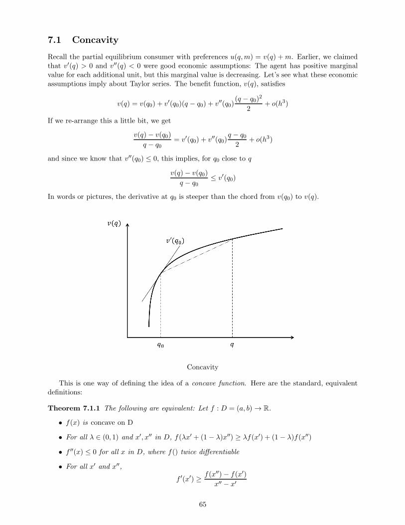
7.1 Concavity

Recall the partial equilibrium consumer with preferences u(q,m) = v(q) +m. Earlier, we claimedthat v′(q) > 0 and v′′(q) < 0 were good economic assumptions: The agent has positive marginalvalue for each additional unit, but this marginal value is decreasing. Let’s see what these economicassumptions imply about Taylor series. The benefit function, v(q), satisfies

v(q) = v(q0) + v′(q0)(q − q0) + v′′(q0)(q − q0)

2

2+ o(h3)

If we re-arrange this a little bit, we get

v(q)− v(q0)

q − q0= v′(q0) + v′′(q0)

q − q02

+ o(h3)

and since we know that v′′(q0) ≤ 0, this implies, for q0 close to q

v(q)− v(q0)

q − q0≤ v′(q0)

In words or pictures, the derivative at q0 is steeper than the chord from v(q0) to v(q).

Concavity

This is one way of defining the idea of a concave function. Here are the standard, equivalentdefinitions:

Theorem 7.1.1 The following are equivalent: Let f : D = (a, b) → R.

• f(x) is concave on D

• For all λ ∈ (0, 1) and x′, x′′ in D, f(λx′ + (1− λ)x′′) ≥ λf(x′) + (1− λ)f(x′′)

• f ′′(x) ≤ 0 for all x in D, where f() twice differentiable

• For all x′ and x′′,

f ′(x′) ≥ f(x′′)− f(x′)

x′′ − x′

65

If the weak inequalities above hold as strict inequalities, then f(x) is strictly concave.

Note that concavity is a global property (holds on all of D) that depends on the domain of thefunction, D = (a, b). For example, log(x) is concave on (0,∞), since

f ′′(x) =−1

x2< 0

for all x in (0,∞). The function√

|x|, however, is concave for (0,∞), and concave for (−∞, 0),but not concave for (−∞,∞). Why? If we connect the points at

√

| ± 1| = 1 by a chord, it liesabove the function at

√

|0| = 0, violating the second criterion for concavity. So a function can havef ′′(x) ≤ 0 for some x and not be concave: It is concave only if f ′′(x) < 0 for all x in its domain,D.

Theorem 7.1.2 If f(x) is differentiable and strictly concave, then it has at most one critical pointwhich is the unique global maximum.

Proof If f(x) is strictly concave, the FONC is

f ′(x) = 0

Since f(x) is strictly concave, the derivative f ′(x) is monotone decreasing. This implies there is atmost one time that f ′(x) crosses zero, so it has at most one critical point. Since

f(x∗)− f(x) = −f ′′(x∗)(x− x∗)2

2> 0

holds (if f ′′(x) < 0 for all x, not just x∗), this is a local maximum. Since there is a unique criticalpoint x∗ and f ′′(x) < 0 for all x, the candidate list consists only of x∗.

There is some room for confusion about what the previous theorem buys you, because a concavefunction might not have any critical points. For example,

f(x) = log(x)

has FONC

f ′(x) =1

x

which reaches f ′(x) = 0 only as x → ∞ (∞ is not a number). Since log(x) → as x → ∞, thereisn’t a finite maximizer. On the other hand

f(x) = log(x)− x

has FONC

f ′(x) =1

x− 1

and SOSC

f ′′(x) = − 1

x2

so that x∗ = 1 is the unique global maximizer.

66

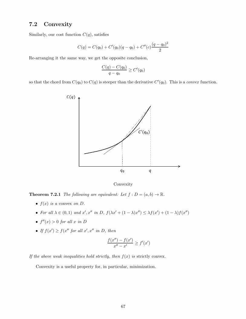
7.2 Convexity

Similarly, our cost function C(q), satisfies

C(q) = C(q0) + C ′(q0)(q − q0) + C ′′(c)(q − q0)

2

2

Re-arranging it the same way, we get the opposite conclusion,

C(q)− C(q0)

q − q0≥ C ′(q0)

so that the chord from C(q0) to C(q) is steeper than the derivative C ′(q0). This is a convex function.

Convexity

Theorem 7.2.1 The following are equivalent: Let f : D = (a, b) → R.

• f(x) is a convex on D.

• For all λ ∈ (0, 1) and x′, x′′ in D, f(λx′ + (1− λ)x′′) ≤ λf(x′) + (1− λ)f(x′′)

• f ′′(x) > 0 for all x in D

• If f(x′) ≥ f(x′′ for all x′, x′′ in D, then

f(x′′)− f(x′)

x′′ − x′≥ f ′(x′)

If the above weak inequalities hold strictly, then f(x) is strictly convex.

Convexity is a useful property for, in particular, minimization.

67

Exercises

1. Rewrite Theorem 7.1.2, replacing the word “concave” with “convex” and “maximization” with“minimization.” Sketch a graph like the first one in the chapter to illustrate the proof.

2. Show that if f(x) is concave, then −f(x) is convex. If f(x) is convex, then −f(x) is concave.

3. Show that if f1(x), f2(x), ..., fn(x) are concave, then f(x) =∑n

i=1 fi(x) is concave. Iff1(x), f2(x), ..., fn(x) are convex, then f(x) =

∑ni=1 fi(x) is convex.

4. Can concave or convex functions have discontinuities? Provide an example of a concave orconvex function with a discontinuity, or show why they must be continuous.

68

Part II

Optimization and ComparativeStatics in R

N

69

Chapter 8

Basics of RN

Now we need to generalize all the key results (extreme value theorem, FONCs/SOSCs, and theimplicit function theorem) to situations in which many decisions are being made at once, sometimessubject to constraints. Since we need functions involving many choice variables and possibly manyparameters, we need to generalize the real numbers to R

N , or N -dimensional Euclidean vectorspace.

An N -dimensional vector is a list of N ordered real numbers,

x =

x1x2...

xN

where certain rules of addition and multiplication are defined. In particular, if x and y are vectorsand a is a real number, scalar multiplication is defined as

ax =

ax1ax2...

axN

and vector addition is defined as

x+ y =

x1 + y1x2 + y2

...xN + yN

The transpose of a column vector is a row vector,

x′ = (x1, x2, ..., xN )

and vice versa. A basis vector ei is a vector with a 1 in the i-th spot, and zeros everywhere else.The set of N -dimensional vectors with real entries R

N is Euclidean, since we define length bythe Euclidean norm. The norm is a generalization of absolute value, and is given by

||x|| =√

x21 + x22 + ...+ x2N

Though, we could just as easily use||x|| = max

ixi

70

or

||x|| =(∑

i

xpi

)1/p

These are all just ways of summarizing how “large” a vector is.

The Norm

For N = 1, this is just R, since ||x|| =√x2 = |x|. With this norm in mind, we define distance

between two vectors x and y as

||x− y|| =√

(x1 − y1)2 + (x2 − y2)2 + ...+ (xN − yN )2

Instead of defining an open interval as (a, b), we define the open ball of radius δ at x0, given by

Bδ(x0) = {y : ||y − x0|| < δ}

and instead of defining a closed interval [a, b], we define the closed ball of radius δ at x0 is

Bδ(x0) = {y : ||y − x0|| ≤ δ}

The last special piece of structure on Euclidean space is vector multiplication, or the innerproduct or dot product :

x′y =< x, y >= x · y = x1y1 + x2y2 + ...+ xNyN

In terms of geometric intuition, the dot product is related to the angle θ between x and y:

cos(θ) =x · y

||x||||y||

Note that if x · y = 0, then cos(θ) = 0, so that the vectors must be at right angles to each other, orx is orthogonal to y.

71

Orthogonal Vectors

So a Euclidean space has notions of direction, distance, and angle, and open and closed ballsare easy to define. Not all spaces have these properties, which makes Euclidean space special1.

8.1 Intervals → Topology

In R, we had open sets (a, b), closed sets [a, b], and bounded sets, where a and b are finite. In multipledimensions, however, it’s not immediately obvious what the generalizations of these propertiesshould be. For example, we could define open cells as sets C = (0, 1)× (0, 1)× ...(0, 1), which looklike squares or boxes. Or we could define open balls as sets B = {y : ||y|| < 1}. But then, we’re goingto study things like budget sets, defined by inequalities like {(x, y) : x ≥ 0, y ≥ 0, pxx+ pyy ≤ w},which are neither balls nor cells.

To avoid these difficulties, we’ll use some ideas from topology. Topology is the study of propertiesof sets, and what kinds of functions preserve those properties. For example, the function f(x) = xmaps the set [−1, 1] into the set [−1, 1], but the function

g(x) =

{

x if |x| 6= 1

0 if |x| = 1

maps [−1, 1] into (−1, 1). So f(x) maps a closed set to a closed set, while g(x) maps a closed setto an open set. So the question, “What kinds of functions map closed sets to closed sets?” is atopological question.

Why do YOU care about topology? What we want to do is study the image of a function,f(D) and see if it achieves its maximum. The function f(x) = x above achieves a maximum atx = 1. The second function, g(x), does not achieve a maximum, since sup g([−1, 1]) = 1 but 1is not in g([−1, 1]). Our one-dimensional Weierstrass theorem tells us that we shouldn’t expectg(x) to achieve a maximum since it is not a continuous function. But how do we generalize thisto Euclidean space and more general sets than simple intervals (right? Because now we might bemaximizing over spheres, triangles, tetrahedrons, simplexes, and all kinds of non-pathological setsthat are more complicated than [a, b])?

1For example, the space of continuous functions over a closed interval [a, b] is also a vector space, called C([a, b]),with scalar multiplication fa = (af(x)), vector addition f + g = (f(x) + g(x)), norm ||f || = maxx∈[a,b] f(x) anddistance d(f, g) = maxx∈[a,b] |f(x) − g(x)|. You use this space all the time when you do dynamic programming inmacroeconomics, since you are looking for an unknown function that satisfies certain properties. This space has verydifferent properties — for example, the closed unit ball {g : d(f, g) ≤ 1} is not compact.

72

Definition 8.1.1 • A set is open if it is a union of open balls

• x is a point of closure of a set S if for every δ > 0, there is a y in S such that ||x− y|| < δ

• The set of all points of closure of a set S is S, and S is the closure of S

• A set S is closed if S = S

• A set S is closed if its complement, Sc is open

• A set S is bounded if it is a subset of an open ball Bδ(x0), where δ is finite. Otherwise, theset is unbounded

Open Balls, Closed Balls, and Points of Closure

Note that x can be a point of closure of a set S without being a member of S. For example, theopen interval (−1, 1) is an open set, since it is an open ball, B1(0) = {y : |y − 0| < 1} = (−1, 1).Each point in B1(0) is a point of closure of (−1, 1), since for all δ > 0 they contain an elementof (−1, 1). However, the points −1 and 1 are also points of closure of (−1, 1), since for all δ > 0,−1 and 1 contain some points of (−1, 1). So the closure of (−1, 1) is [−1, 1]. As you might haveexpected, this is a closed set.

This works just as well in Euclidean space. The open ball at zero, Bδ(0) = {y : ||y − 0|| < δ}is an open ball, so it is a union of open balls, so it is open. All elements of Bδ(0) are points ofclosure of Bδ(0), since for all δ > 0, they contain a point of Bδ(0). However, the points satisfying{y : ||y − 0|| = δ} are also points of closure, since part of the open ball around any of thesepoints must intersect with Bδ(0). Consequently, the set of all points of closure of Bδ(0) is the set{y : ||y − 0|| ≤ δ}, which is the closed ball.

There are many other properties that are considered topological: connected, dense, convex,separable, and so on. But for our purposes of developing maximization theory, there is a specialtopological property that will buy us what we need to generalize the extreme value theorem:

73

Definition 8.1.2 A subset K of Euclidean space is compact if each sequence in K has a subse-quence that converges to a point in K.

The Bolzano-Weierstrass theorem (which is a statement about the properties of sequences)looks similar, but this definition concerns the properties of a sets. A set is called compact if anysequence constructed from it has the Balzano-Weierstrass property. For example, the set (a, b)is not compact, because xn = b − 1/n is a sequence entirely in (a, b), but all of its subsequencesconverge to b which is not in (a, b). Characterizing compact sets in a space is the typical startingpoint for studying optimization in that space2. As it happens, there is an easy characterization forRN :

Theorem 8.1.3 (Heine-Borel) In Euclidean space, a set is compact iff it is closed and bounded.

Basically, bounded sets that include all their points of closure are compact in RN . Non-compact

sets are either unbounded, like {(x, y) : (x, y) ≥ (0, 0)}, or open, like {(x, y) : x2 + y2 < c}.

Example Consider the set in RN described by xi ≥ 0 for all i = 1, ..., N , and

N∑

i=1

pixi = p · x ≤ w

This is called a budget set, Bp,w. In two dimensions, this looks like a triangle with vertices at 0,w/p1 and w/p2. This set is compact.

We’ll use the Heine-Borel theorem, and show the set is closed and bounded.

Budget Sets

It is bounded, since if we take δ = maxi w/pi + 1, the set is contained in Bδ(0) (right?). It isclosed since if we take any sequence xn satisfying xn ≥ 0 for all n and p ·xn ≤ w for all n, the limitof the sequence must satisfy these inequalities as well (a weakly positive sequence for all terms can’tbecome negative at the limit). If you don’t like that argument that it is closed, we can prove Bp,w

is closed by showing that the complement of Bp,w is open: Let y be a point outside Bp,w. Thenthe ray z = α0 + (1− α)y where α ∈ [0, 1] starts in the budget set, but eventually exits it to reachy. Take α∗ to be the point at which the ray exits the set. Then we can draw an open ball aroundy with radius r = (1 − α∗)/2, so that Br(y) contains no points of Bp,w. That means that for anyy, we can draw an open ball around it that contains no point in Bp,w. That means that Bc

p,w is aunion of open balls, so Bp,w is closed.

2See the footnote on page 1: Closed, bounded sets in C([a, b]) are not compact.

74

So competitive budget sets are compact. In fact, we’ve shown that any set characterized byx ≥ 0 and a · x ≤ c is compact, which is actually a sizeable number of sets of interest.

Example The N -dimensional unit simplex, ∆N is constructed by taking the N basis vectors,(e1, e2, ..., en), and considering all convex combinations

xλ = λ1e1 + λ2e2 + ...+ λNeN

such that∑N

i=1 λi = 1 and 0 ≤ λi ≤ 1.Then ∆N is bounded, since if we take the N -dimensional open ball B2(0) of radius 2, it includes

the simple. And ∆N is closed, since, taking any sequence λn → λ, and limn→∞ λ′n(e1, ..., eN ) =

λ′(e1, ..., eN ), which is in the simplex. So the simplex is its own closure, ∆N = ∆N , so it is closed.

The simplex comes up in probability theory all the time: It is the set of all probability distri-butions over N outcomes.

8.2 Continuity

Having generalized the idea of “[a, b]” to RN , we now need to generalize continuity. Continuity is

more difficult to visualize in RN since we can no longer sketch a graph on a piece of paper. For

a function f : R2 → R we can visualize the graph in three dimensions. A continuous function isone for which the “sheet” is relatively smooth: It may have “ridges” or “kinks” like a crumpled-uppiece of paper that has been smoothed out, but there are no “rips” or “tears” in the surface.

Definition 8.2.1 A function f : D → R is continuous at c ∈ D if for all ε > 0, there exists aδ > 0 so that if ||x− c|| < δ, then |f(x)− f(c)| < ε.

The only modification from the one-dimensional definition is that we have replaced the set(c − δ, c + δ) with an open ball, Bδ(c) = {x : ||x − c|| < δ}. Otherwise, everything is the same.Subsequently, the proof of the Sequential Criterion for Continuity is almost exactly the same:

Theorem 8.2.2 (Sequential Criterion for Continuity) A function f : D → R is continuousat c iff for all sequences xn → c, we have

limn→∞

f(xn) = f(

limn→∞

xn

)

= f(c)

Again, continuity allows us to commute the function f() with a limit operator lim. This is thelast piece of the puzzle of generalizing the extreme value theorem.

8.3 The Extreme Value Theorem

So, what do you have to internalize from the preceding discussion in this chapter?

• A set is open if it is a union of open balls.

• A set is closed if it contains all its points of closure. A set is closed if its complement is open.

• A set is compact in RN if it is closed and bounded.

• In compact sets, all sequences have a convergent subsequence.

75

• If a function is continuous in RN , then

limn→∞

f(xn) = f(

limx→∞

xn

)

for any sequence xn → c.

The above facts let us generalize the Extreme Value Theorem:

Theorem 8.3.1 (Weierstrass’ Extreme Value Theorem) If K is a compact subset of RN andf : K → R is a continuous function, then f(x) achieves a maximum on K.

Proof Letsup f(K) = m∗

Then we can construct a sequence xn satisfying

m∗ − 1

n≤ f(xn) ≤ m∗

Since K is compact, every sequence xn has a convergent subsequence xnk→ x∗. Taking limits

throughout the inequality, we get

limnk→∞

m∗ − 1

nk≤ lim

nk→∞f(xnk

) ≤ m∗

and by continuity of f(),

limnk→∞

m∗ − 1

nk≤ f

(

limnk→∞

xnk

)

≤ m∗

so thatm∗ ≤ f(x∗) ≤ m∗

Since K is closed, the limit x∗ of the convergent subsequence xnkis in K (See the proof appendix;

all closed sets contain all of their limit points).Therefore, a maximizer exists since x∗ is in K and achieves the supremum, f(x∗) = m∗.

This is the key result in explaining when maximizers and minimizers exist in RN . Moreover,

the assumptions are generally easy to verify: Compact sets are closed and bounded, which we caneasily find in Euclidean space, and since our maximization problems generally involve calculus, f(x)will usually be differentiable, which implies continuity.

8.4 Multivariate Calculus

As we discussed earlier, differentiability of a function f : RN → R is slightly more complicated thatfor the one-dimensional case. We review some of that material here briefly and introduce some newconcepts.

Definition 8.4.1 • The partial derivative of f(x) with respect to xi, where f : D → R and Dis an open subset of R, is

∂f(x)

∂xi= fxi

(x) = limh→0

f(x1, x2, ..., xi−1, xi + h, xi+1, ..., xN )− f(x1, x2, ..., xi−1, xi, xi+1, ..., xN )

h

• The gradient of f(x) is the vector of partial derivatives,

∇f(x) =

(∂f(x)

∂x1,∂f(x)

∂x2, ...,

∂f(x)

∂xN

)

76

• The total differential of f(x) at x is

df(x) =N∑

i=1

fxi(x)dxi

Now that we have a slightly better understanding of RN , the geometric intuition of the gradientis more clear. The partial derivative with respect to xi is a one-dimensional derivative in the i-thdimension, giving the change in the function value that can be attributed to perturbing xi slightly.The gradient is just the vector from the point (x, f(x)) pointing in the direction ∇f(x), whichrepresents how the function is changing at that point.

If we multiple ∇f(x) by the basis vector ei — where ei = 1 in the i-th entry, but is zerootherwise — we get

∇f(x) · ei =∂f(x)

∂xiso we are asking, “If we increase xi a small amount, how does f(x) change?” What if we wantedto investigate how f(x) changes in some other direction, y? The change in f(x) in the direction yhas h goes to zero is given by

limh→0

f(x1 + y1h, ..., xN + yNh)− f(x1, ...xN )

h

To compute this, we can use a Taylor series dimension-by-dimension on f(x1 + y1h, x2 + y2h) toget

f(x1 + y1h, x2 + y2h) = f(x1, x2 + y2h) +∂f(ξ1, x2 + y2h)

∂x1y1h

where ξ1 is between x1 and x1 + y1h. Doing this again with respect to x2 gives

f(x1, x2 + y2h) = f(x1, x2) +∂f(x1, ξ2)

∂x2y2h

Substituting the above equation into the previous one yields

f(x1 + y1h, x2 + y2h) = f(x1, x2) +∂f(x1, ξ2)

∂x2y2h+

∂f(ξ1, x2 + y2h)

∂x1y1h

Re-arranging and dividing by h yields

f(x1 + y1h, x2 + y2h)− f(x1, x2)

h=

∂f(ξ1, x2 + y2h)

∂x1y1 +

∂f(x1, ξ2)

∂x2y2

Since x1 + y1h → x1 as h → 0, ξ1 → x1 and ξ2 → x2. Then taking limits in h yields

Dyf(x) =∂f(x1, x2)

∂x1y1 +

∂f(x1, x2)

∂x2y2

Note that even through y is not an “infinitesimal vector”, this is the differential change in the valueof f(x) with respect to an infinitesimal change in x in the direction y. In general,

Theorem 8.4.2 The change in f(x) in the direction y is given by the directional derivative off(x) in the direction y,

Dyf(x) =

N∑

i=1

∂f(x)

∂xiyi

orDyf(x) = ∇f(x) · y

This is certainly useful for maximization purposes: You should anticipate that x∗ is a localmaximum if, for any y, Dyf(x

∗) = 0. Notice also that the total differential df(x), is just thedirection derivative with respect to the unit vector e = (dx1, dx2, ..., dxN ), or

df(x) = ∇f(x) · dx

77

The Hessian

The gradient only generalizes the first derivative, however, and our experience from the one-dimensional case tells us that the second derivative is also important. But Exercise 8 from Chapter4 suggests that the vector of second partial derivatives of f(x) is not sufficient to determine whethera point is a local maximum or minimum. The correct generalization of the second derivative is notanother vector, but a matrix.

Definition 8.4.3 The Hessian of f(x) is the matrix

∂2f(x)

∂x21

∂2f(x)

∂x1∂x2. . .

∂2f(x)

∂xN∂x1∂2f(x)

∂x2∂x1

∂2f(x)

∂x22...

. . .

∂2f(x)

∂xN∂x1

∂2f(x)

∂x2N

Various notations for the Hessian are ∇2xf(x), D

2f(x), ∇xx = ∇x · ∇′x, and H(x).

For notational purposes, it is sometimes easier to write the matrix

∇xx =

∂2

∂x21

∂2

∂x1∂x2. . .

∂2

∂xN∂x1∂2

∂x2∂x1

∂2

∂x22...

. . .

∂2

∂xN∂x1

∂2

∂x2N

and think of the Hessian as ∇xx ∗ f(x) = H(x). In particular, ∇xx = ∇x · ∇′x, so that when you

take the “gradient of a gradient” you get a Hessian.To begin understanding this matrix, consider the quadratic form,

f(x1, x2) = a1x1 + a2x2 +1

2b112x

21 +

1

2b22x

22 + b3x1x2 + c

This is the correct generalization of a quadratic function bx2 + ax+ c to two dimensions, allowinginteraction between the x1 and x2 arguments. It can be written as

f(x) = a′x+1

2x′Bx+ c

where a = [a1, a2]′ and

B =

[b11 b3b3 b22

]

By increasing the rows and columns of a and H, this can easily be extended to mappings from RN

for any N .The gradient of f(x1, x2) is

∇f(x) =

[a1 + b11x1 + b3x2a2 + b22x2 + b3x1

]

78

But you can see that x2 appears in fx1(x), and vice versa, so that changes in x2 affect the partialderivative of x1. To summarize this information, we need the extra, off-diagonal terms of theHessian, or

H(x) =

[b11 b3b3 b22

]

= B

A basic fact of importance is that the Hessian is symmetric matrix when f(x) is continuous, oror H ′ = H:

Theorem 8.4.4 (Young’s Theorem) If f(x) is a continuous function from RN → R, then

∂2f(x)

∂xi∂xj=

∂2f(x)

∂xj∂xi

and more generally, the order of partial differentiation can be interchanged arbitrarily for all higher-order partial derivatives.

8.5 Taylor Polynomials in Rn

Second-order approximations played a key role in developing second-order sufficient conditionsfor the one-dimensional case, and we need a generalization of them for the multi-dimensionalcase. Again, however, the right “generalization” is somewhat subtle. The second-order Taylorpolynomials of the one-dimensional case were quadratic functions with an error term,

f(x) = f(x0) + f ′(x0)(x− x0) + f ′′(x0)(x− x0)

2

2+ o(h3)

In the multi-variate case, we start with a quadratic function,

f(x) = c+ a′x+1

2x′Bx

and replace each piece with its generalization of the one-dimensional derivative and second deriva-tive to get a quadratic approximation

f(x) = f(x0) +∇f(x0)(x− x0) + (x− x0)′H(x0)

2(x− x0)

and this quadratic approximation becomes a Taylor polynomial when we add the remainder/errorterm, o(h3):

f(x) = f(x0) +∇f(x0)(x− x0) + (x− x0)′H(x0)

2(x− x0) + o(h3)

where h = x− x0.

Definition 8.5.1 Let f : D → R be a thrice-differentiable function, and D an open subset of RN .Then the second-order Taylor polynomial of f(x) at x0 is

f(x) = f(x0) +∇f(x0)(x− x0) +1

2(x− x0)

′H(x0)(x− x0) + o(h3)

where h = x− x0, and the remainder o(h3) → 0 as x → x0.

A linear approximation of f around a point x0 is the function

f(x) = f(x0) +∇f(x0)(x− x0)

and a quadratic approximation of f around a point x0 is the function

f(x) = f(x0) +∇f(x0)(x− x0) + (x− x0)′H(x0)

2(x− x0)

Higher-order approximations require a lot more notation, but second-order approximations are allwe need.

79

8.6 Definite Matrices

In the one dimensional case, the quadratic function

f(x) = c+ ax+Ax2

was well-behaved for maximization purposes when it had a negative second derivative, or A < 0.In the multi-variate case,

f(x) = c+ a · x+1

2x′Ax

it is unclear what signx′Ax

takes. For instance, a ·x > 0 if a ≥ 0 and x ≥ 0. But when is x′Ax ≥,≤, >,< 0? If we knew this, itwould be easier to pick out “nice” optimization problems, just as we know that the one-dimensionalfunction f(x) = Ax2 + ax+ c will only have a “nice” solution if A < 0.

We can easily pick out some matrices A so that x′Ax < 0 for all x ∈ RN . If

A =

a1 0 0 00 a2 0 0

0 0. . . 0

0 0 0 aN

then x′Ax =∑N

i=1 aix2i , and this will only be negative if each ai < 0. Notice that,

1. The eigenvalues of A are precisely the diagonal terms a1, ..., aN

2. The absolute value of ai is greater than the sum of all the off-diagonal terms (which is zero)

3. If we compute the determinant of each sub-matrix starting from the upper left-hand corner,the determinants will alternate in sign

These are all characterizations of a negative definite matrix, or one for which x′Ax < 0 for all x.But once we start adding off-diagonal terms, this all becomes much more complicated because it isno longer sufficient merely to have negative terms on the diagonal. Consider the following matrix:

A =

[−1 −2−2 −1

]

All the terms are negative, so many students unfamiliar with definite matrices think that x′Axwill then be negative, as an extension of their intuitions about one-dimensional quadratic formsax2 + bx. But this is false. Take the vector x = [1,−1]:

x′Ax = [1,−1]′[1,−1] = 1 + 1 = 2 > 0

The failure here is that the quadratic form x′Ax = −x21 + −x22 − 4x1x2 looks like a “saddle”, notlike a “hill”. If x1x2 < 0, then −4x1x2 > 0, and this can wipe out −x21 − x22, leaving a positivenumber. So a negative definite matrix must have a negative diagonal, and the “contribution” ofthe diagonal terms will outweigh those of the off-diagonal terms.

Let A be a N ×N matrix, and x = (x1, x2, ..., xn) a vector in RN . A quadratic form on R

N isthe function

x′Ax =

N∑

i=1

N∑

j=1

aijxixj

80

Definition 8.6.1 Let A be an n× n symmetric matrix. Then A is

• positive definite if, for any x ∈ Rn\0, x′Ax > 0

• negative definite if, for any x ∈ Rn\0, x′Ax < 0

• positive semi-definite if, for any x ∈ Rn\0, x′Ax ≥ 0

• negative semi-definite if, for any x ∈ Rn\0, x′Ax ≤ 0

Why does this relate to optimization theory? When maximizing a multi-dimensional function,a local (second-order Taylor) approximation of it around a point x∗ should then look like a hill ifx∗ is a local maximum. If, locally around x∗, the function looks like a saddle or a bowl, the valueof the function could be increased by moving away from x∗. So these tests are motivated by theconnections between the geometry of maximization and quadratic forms. In short, these definitionsgeneralize the idea of a positive or negative number in R to a “positive or negative matrix”.

Definition 8.6.2 The leading principal minors of a matrix A are the matrices,

A1 = a11

A2 =

[a11 a12a21 a22

]

...

An =

a11 a12 . . . a1n

a21 a22...

......

.... . .

...an1 an2 . . . ann

Here are the main tools for characterizing definite matrices:

Theorem 8.6.3 Let A be an n× n symmetric matrix. Then A is negative definite if

• All the eigenvalues of A are negative

• The leading principal minors of A alternate in sign, starting with det(A1) < 0

• The matrix has a negative dominant diagonal: For each row r,

|arr| >

∣∣∣∣∣∣

∑

i 6=r

ari

∣∣∣∣∣∣

and arr < 0.

Example Consider

A =

[−2 11 −2

]

The leading principal minors are −2 < 0 and 4− 1 = 3 > 0, so this matrix is negative definite.The eigenvalues are found by solving

det(A− λI) = (−2− λ)2 − 1 = 0

and λ∗ = −2± 1 < 0. So the eigenvalues of A are all negative.Since 2 > 1, it has the dominant diagonal property.

81

Example Consider

A =

[−1 −2−2 −1

]

The leading principal minors are −1 < 0 and 1− 4 < 0, so this matrix is not negative definite.The eigenvalues are found by solving

det(A− λI) = λ2 + 2λ− 3 = 0

and λ∗ = −1± 2. It is not negative definite since it has an eigenvalue 1 > 0.The principal minors test is obviously not satisfied.Since A is neither negative nor positive (semi-)definite, it is actually indefinite.

These tests seem “magical”, so it’s important to develop some intuition about what they mean.

• If H is a real symmetric matrix, it can be factored into an orthogonal matrix P and a diagonalmatrix D where

H = PDP ′

and the eigenvalues (λ1, λ2, ...λn) of H are on the diagonal. If we do this,

x′Hx = x′PDP ′x = (x′P )D(P ′x) = (P ′x)′D(P ′x)

Note that P ′x is a vector; call it y. Then we get

y′Dy =∑

ℓ

y2i λi

If all the eigenvalues λi of H are negative, the y2i terms are positive scalars, and we canconclude x′Hx < 0 if and only if H has all strictly negative eigenvalues.

• How can the principal minors test be motivated? We can get a feel for why this mustbe true from the following observations: (i) If x′Hx < 0 for all x, then if we use x =(x1, x2, ..., xk, 0, ..., 0), with not all components zero, then x′Hx < 0 as well. But because ofthe zeros, we’re really just considering a k×k sub-matrix of H, Hk. (ii) The determinant of amatrix A is equal to the product of its eigenvalues. So if we take H1, the determinant is h11,and that should be negative; det(H2) = λ1λ2, which should be positive ifH is negative definite(since the determinant is the product of the eigenvalues, and we know that the eigenvaluesof a negative definite matrix are negative) ; det(H3) = λ1λ2λ3 < 0; and so on. So combiningthese two facts tells us that if H is negative definite, then we should observe this alternativesign pattern in the determinants of the principal minors. (Note that this only shows that ifH is negative definite, then the principal minors test holds, not the converse.)

• Necessity of the dominant diagonal theorem is easy to show, but sufficiency is much harder.Suppose H is negative definite. Take the set of vectors 1 = (1, 1, ..., 1), and observe thequadratic form

1′H1 =∑

i

∑

j

hij < 0

Now, if for each row i, we had∑

j hij < 0, the above inequality holds, since we then just sumover all i. But this is equivalent to

hii +∑

j 6=i

hji < 0

82

Re-arranging yields

hii < −∑

j 6=i

hji

Multiplying by −1 yields

−hii >∑

j 6=i

hji

and taking absolute values yields

|hii| >

∣∣∣∣∣∣

∑

j 6=i

hji

∣∣∣∣∣∣

which is the dominant diagonal condition.

There are other tests and conditions available, but these are often the most useful in practice.Note that it is harder to identify negative semi-definiteness, because the only test that still appliesis that all eigenvalues be weakly negative. In particular, if all the determinants of the principalminors alternate in sign but are sometimes zero, the quadratic form might be a saddle, similar tof(x) = x3 being indefinite at x = 0, with f ′′(x) = 6x.

Exercises

1. Show that RN is both open and closed. Show that the union and intersection of any collection ofclosed sets is closed. Show that the union of any collection of open sets is open, and the intersectionof a finite number of open sets is open. Show that a countable intersection of open sets can beclosed.

2. Determine if the following matrices are positive or negative (semi)-definite:

[−1 30 −1

]

[−1 11 −1

]

[−1 53 −10

]

1 −2 1−2 4 −21 −2 1

3. Find the gradients and Hessians of the following functions, evaluate the Hessian at the pointgiven, and determine whether it is positive or negative (semi-)definite. (i) f(x, y) = x2 +

√x at

(1, 1). (ii) f(x, y) =√xy at (3, 2), and any (x, y). (iii) f(x, y) = (xy)2 at (7, 11) and any (x, y).

(iv) f(x, y, z) =√xyz at (2, 1, 3).

4. Give an example of a matrix that has all negative entries on the diagonal but is not negativedefinite. Give an example of a matrix that has all negative entries but is not negative definite.

5. Prove that a function is continuous iff the inverse image of an open set is open, and theinverse image of a closed set is closed. Prove that if a function is continuous, then the image of abounded set is bounded. Conclude that a continuous function maps compact sets to compact sets.Use this to provide a second proof of the extreme value theorem.

83

Proofs

The proofs here are mostly about compactness and the Heine-Borel theorem.

Definition 8.6.4 A subset K of Euclidean space is compact if each sequence in K has a subse-quence that converges to a point in K.

So a set is compact3 if the Bolzano-Weierstrass theorem holds for every sequence constructedonly from points in the set. For an example of a non-compact set, consider (a, b). The sequencexn = b− 1/n is constructed completely from points in (a, b), but its limit, b, is not in the set, so itdoes not have the Bolzano-Weierstrass property.

Recall that in our proof of the Weierstrass theorem, we insured a maximum existed by studyingconvergent sub-sequences. This will be the key to again ensuring existence in the N -dimensionalcase. The next proof theorem characterizes “closedness” in terms of sequences.

Theorem 8.6.5 Suppose xn is a convergent sequence such that xn is in S for all n. Then xnconverges to a point in the closure of S, S.

Proof (Sketch a picture as you go along). Suppose, by way of contradiction, that x is not in S.Then we can draw an open ball around x of radius ε > 0 such that no points of S are in Bε(x).But since xn → x, we also know that for all ε > 0, for n ≥ H, ||xn − x|| < ε, so that countablymany points of S are in Bε(x). This is a contradiction.

Since a closed set satisfies S = S, this implies that every sequence in a closed set — if itconverges — converges to a member of the set. However, there are sets like [0,∞) that are closed— since any sequence that converges in this set converges to a point of the set — but allow plentyof non-convergent sequences, like xn = n. For example, if you were asked to maximize f(x) = xon the set [b,∞), no maximum exists: f([b,∞)) = [b,∞), and the range is unbounded. So formaximization theory, it appears that closedness and boundedness of the image of a set under afunction are key properties. In fact, they are equivalent to compactness in R

N .

Theorem 8.6.6 (Heine-Borel) In Euclidean space, a set is compact iff it is closed and bounded.

Proof Consider any sequence xn in a closed and bounded subset K of RN . We will show it has aconvergent subsequence, and consequently that K is compact.

Since K is bounded, there is a N -dimensional “hypercube” H, which satisfies H = ×Ni=1[ai, bi]

and K ⊂ H. Without loss of generality we can enlarge the hypercube to [a, b]N , where a = mini aiand b = maxi bi, so that bi − ai is the same length for all dimensions.

Now cut H in N2 equally sized sets, each of size ((b− a)/N)N . One of these cubes contains aninfinite number of terms of the sequence in K. Select a term from that cube and call it xn1 , andthrow the rest of the cubes away. Now repeat this procedure, cutting the remaining cube N waysalong each dimensions; one of these sub-cubes contains an infinite number of terms of the sequence;select a term from that subcube and call it xnk

, and throw the rest away.The volume of the subcubes at each step k is equal to

(b− a)N

Nk

3The most general definition of compactness is, “A subset K of Euclidean space is compact if any collection ofopen sets {Oi}

∞

i=1 for which K ⊂ ∪iOi has a finite collection {Oik}Kk=1 so that K ⊂ ∪K

k=1Oik”, which is converted intowords by saying, “K is compact if every open cover of K — K ⊂ ∪∞

i=1Oi — has a finite sub-cover — K ⊂ ∪Kk=1Oik”,

or that if an infinite collection of open sets covers K, we can find a finite number of them that do the same job. Thisis actually easier to work with than the sequential compactness we’ll use, but they are equivalent for N .

84

which is clearly converging to zero as k → ∞. Then a bound on the distance from each term to alllater terms in the sequence is given by the above estimate.

Therefore, the sequence constructed from this procedure has a limit, x (since it is a Cauchysequence). Therefore, the subsequence xnk

converges. Since K is closed, it contains all of its limitpoints by Theorem 8.8.2 above, so x is an element of K. Therefore K is compact.

The Bolzano-Weierstrass theorem was a statement about bounded sequences: Every boundedsequence has a convergent subsequence. The Heine-Borel theorem is a statement about closed andbounded sets: A set is compact iff it is closed and bounded. The bridge between the two is thatan infinitely long sequence in a bounded set must be near some point x infinitely often. If the setcontains all of its points of closure, this point x is actually a member of the set K, and compactnessand boundedness are closely related. However, boundedness is not sufficient, since a sequence mightnot converge to a point in the set, like the case (a, b) with b − 1/n. To ensure the limit is in theset, we add the closedness condition, and we get a useful characterization of compactness.

85

Chapter 9

Unconstrained Optimization

We’ve already seen some examples of unconstrained optimization problems. For example, a firmwho faces a price p for its good, hired capital K and labor L at rates r and w per unit, and pro-duces output according to the production technology F (K,L) faces an unconstrained maximizationproblem

maxK,L

pF (K,L)− rK −wL

In this and similar problems, we usually allow the choice set to be RN , and allow the firm to pick

any K and L that maximizes profits. As long as K and L are both positive, this is a fine approach,and we don’t have to move to the more complicated world of constrained optimization.

Similarly, many constrained problems have the feature that the constraint can be re-written interms of one of the controls, and substituted into the objective. For example, in the consumer’sproblem

maxx

u(x)

subject to w = p · x, the constraint can be re-written as

xN =w −∑ i = 1N−1pixi

pN

and substituted into the objective to yield

maxx1,...,xN−1

u

(

x1, ..., xN−1,w −∑ i = 1N−1pixi

pN

)

which is an unconstrained maximization problem in x1, ..., xN−1. Even though we have bettermethods in general for solving the above problem from a theoretical perspective, solving an uncon-strained problem numerically is generally easier that solving a constrained one.

Definition 9.0.7 Let f : Rn → R, x ∈ Rn. Then the unconstrained maximization problem is

maxx∈RN

f(x)

A global maximum of f on X is a point x∗ so that f(x∗) ≥ f(x′) for all other x′ ∈ X. A point x∗

is a local maximum of f if there is an open set S = {y : ||x− y|| < ε} for which f(x∗) ≥ f(y) forall y ∈ S.

How do we find solutions to this problem?

86

9.1 First-Order Necessary Conditions

Our first step to solving unconstrained maximization problems is to build up a candidate list usingFONCs, just like in the one-dimensional case.

Definition 9.1.1 If ∇f(x∗) = 0, then x∗ is a critical point of f(x).

Example Recall the firm with profit function

π(K,L) = maxK,L

pF (K,L) − rK −wL

Then if we make a small change in K, the change in profits is

∂π(K,L)

∂K= pFK(K,L) − r

and if we make a small change in L, the change in profits is

∂π(K,L)

∂L= pFL(K,L)− w

If there are no profitable adjustments away from a given point (K∗, L∗), then it must be a localmaximum, so the equations above both equation zero. But then ∇π(K∗, L∗) = 0 implies that(K∗, L∗) is a critical point of f(x).

The above argument works for any function f(x):

Theorem 9.1.2 (First-Order Necessary Conditions) If x∗ is a local maximum of f and f isdifferentiable at x∗, then x∗ is a critical point of f .

Proof If x∗ is a local maximum and f is differentiable at x∗, there cannot be any improvement inany direction v 6= 0. The directional derivative is

∇f(x∗) · v =∑

i

∂f(x∗)

∂xivi

So we can think of the differential change as the sum of one-dimensional directional derivatives inthe direction y = (0, ..., vi, 0, ..., 0) where y is zero except for the i-th slot, taking the value vi 6= 0:

∇f(x∗) · y =∑

i

∂f(x∗)

∂xivi =

∂f(x∗)

∂xivi = 0

So that each partial derivative must be zero along each dimension individually, implying that alocal maximum is a critical point.

Like in the one-dimensional case, this gives us a way of building a candidate list of potentialmaximizers: Critical points and any points of non-differentiability.

Example Consider a quadratic objective function,

f(x1, x1) = a1x1 + a2x2 −b12x21 −

b22x22 + cx1x2

The FONCs area1 − b1x

∗1 + cx∗2 = 0

87

a2 − b2x∗2 + cx∗1 = 0

Any solution to these equations is a critical point. If we solve the system by hand, the secondequation is equivalent to

x∗2 =a2 + cx∗1

b2

and substituting it into the first gives

a1 − b1x∗1 + c

a2 + cx∗1b2

= 0

or

x∗1 =a1b2 + a2c

b1b2 − c2

x∗2 =a2b1 + a1c

b1b2 − c2

If, instead, we convert this to a matrix equation,

[a1a2

]

+

[−b1 cc −b2

] [x∗1x∗2

]

= 0

Re-arranging yields

−[−b1 cc −b2

] [x∗1x∗2

]

=

[a1a2

]

Which looks exactly like −Bx∗ = a. From linear algebra, we know that there is a solution as longas B is non-singular (it has full rank ↔ all its eigenvalues are non-zero ↔ it is invertible ↔ it hasnon-zero determinant). Then

x∗ = (−B)−1a

and we have a solution. The determinant of B is non-zero iff

b1b2 − c2 6= 0

So if the above condition is satisfied, there is a unique critical point.Notice, however, that we could have done the whole analysis as

f(x) = ax+ x′B

2x

yielding FONCsa+Bx∗ = 0

orx∗ = −B−1a

Moreover, this equation can be solved in a few lines of Matlab code, making it useful starting pointfor playing with non-linear optimization problems. However, we still don’t know know whether x∗

is a maximum, minimum, or saddle point.

88

9.2 Second-Order Sufficient Conditions

With FONCs, we can put together a candidate list for any unconstrained maximization problem:Critical points and any points of non-differentiability. However, we still don’t know whether a givencritical point is maximum, minimum or saddle/inflection point.

Example Consider the functionf(x, y) = −x2y

The FONCs for this function arefx(x, y) = −2xy = 0

fy(x, y) = −x2 = 0

The unique critical point is (0, 0). But if we evaluate the function at (1,−1), we get f(1,−1) =−(1)(−1) = 1 > 0 = f(0, 0). What is going on? Well, if we were considering −x2 alone, it wouldhave a global maximum at zero. But the y term has no global maximum. When you multiplythese functions together, even though one is well-behaved, the mis-behavior of the other leads tonon-existence of a maximizer in R

2 (I can make f(x, y) arbitrarily large by making y arbitrarilynegative and x = 1).

Still worse, as you showed in Exercise 8 of Chapter 4, it is not enough that a critical point(x∗, y∗) satisfy fxx(x

∗, y∗) < 0 and fyy(x∗, y∗) < 0 to be a local maximum.

Example Consider the function

f(x, y) = −1

2x2 − 1

2y2 + bxy

where b > 0. The FONCs arefx(x, y) = −x+ by = 0

fy(x, y) = −y + bx = 0

The unique critical point of the system is (0, 0). However, if we set x = y = z, the function becomes

f(z) = −z2 + bz2

and if b > −1, we can make the function arbitrarily large. The function is perfectly well behavedin each direction: If you plot a cross-section of the function for all x setting y to zero, it achieves amaximum in x at zero, and if you plot a cross-section of the function for all y setting x to zero, itachieves a maximum in y at zero. Nevertheless, this is not a global maximum if b is too large.

If we use a Taylor series, however, we can write any multi-dimensional function as

f(x) = f(x0) +∇f(x0) · (x− x0) + (x− x0)′H(x0)

2(x− x0) + o(h3)

If x∗ is a critical point, we know that ∇f(x∗) = 0, or

f(x) = f(x∗) + (x− x∗) · H(x∗)

2(x− x∗) + o(h3)

and re-arranging yields

f(x∗)− f(x) = −(x− x∗) · H(x∗)

2(x− x∗)− o(h3)

89

Letting h = x − x∗ be arbitrarily close to zero and noting that if x∗ is a local maximum of f(x),we then have

f(x∗)− f(x) = −(x− x∗) · H(x∗)

2(x− x∗) > 0

Or that, for any vector y,y′H(x∗)y < 0

This is the definition of a negative definite matrix, giving us a workable set of SOSCs for multi-dimensional maximization:

Theorem 9.2.1 (Second-Order Sufficient Conditions) If x∗ is a critical point of f(x) and H(x∗)is negative definite, then x∗ is a local maximum of f(x).

For example, the Hessian for

f(x, y) = −1

2x2 − 1

2y2 + bxy

is [−1 bb −1

]

The determinant of the Hessian is 1 − b2, which is positive if b < 1. So if b is sufficiently small,f(x, y) will have a local maximum at (0, 0).

On the other hand, if we start with the assumption that x∗ is a local maximum of f(x) and notjust a critical point, using our Taylor series approximation, we get

f(x∗)− f(x) = −(x− x∗)′H(x∗)

2(x− x∗) + o(h3)

Since x∗ is a local maximum, we know that f(x∗) ≥ f(x), so that

−(x− x∗)′H(x∗)

2(x− x∗) ≥ 0

for x sufficiently close to x∗, implying that y′H(x∗)y ≤ 0. This is negative semi -definiteness.To summarize:

Theorem 9.2.2 (Second-Order Sufficient Conditions) Let f : Rn → R be a twice differen-tiable function, and let x∗ be a point in R

n.

• If x∗ is a critical point of f(x) and H(x∗) is negative definite, then x∗ is a local maximum off .

• If x∗ is a critical point of f(x) and H(x∗) is positive definite, then x∗ is a local minimum off .

• If f has a local maximum at x∗, then H(x∗) is negative semi-definite.

• If f has a local minimum at x∗, then H(x∗) is positive semi-definite.

The first two points are useful for checking whether or not a particular point is a local maximumor minimum. The second two are useful when using the implicit function theorem.

Here are some examples:

90

Example Suppose a price-taking firm gets a price p for its product, which it produces usingcapital K and labor L and technology F (K,L) = q. Capital costs r per unit and labor costs w perunit. This gives a profit function of

π(K,L) = pF (K,L) − rK − wL

The FONCs arepFK(K,L) − r = 0

pFL(K,L) −w = 0

And our SOSCs are that [FKK(K∗, L∗) FKL(K

∗, L∗)FLK(K∗, L∗) FLL(K

∗, L∗)

]

be a negative-definite matrix. This implies

FKK(K∗, L∗) < 0

FLL(K∗, L∗) < 0

andFKK(K∗, L∗)FLL(K

∗, L∗)− FKL(K∗, L∗)2 > 0

So F (K,L) must be own-concave in K and L, or FKK(K∗, L∗) < 0 and FLL(K∗, L∗) < 0.

Likewise, the cross-partial FKL(K∗, L∗) cannot be “too large”. In terms of economics, K and L

cannot be such strong substitutes or complements that switching from one to the other has a largerimpact than using more of each. A simple example might be

F (K,L) = a1K − a22K2 + b1L− b2

2L2 + cKL

Our Hessian would then be [−a2 cc −b2

]

with determinanta2b2 − c2 > 0

So that (K∗, L∗) is a local maximum if√a2b2 > c.

Example Slightly different firm problem: A firm hires capital K at rental rate r and labor L atwage rate w. The firm’s output produced by a given mix of capital and labor is F (K,L) = φKαLβ.The price of the firm’s good is p. This is an unconstrained maximization problem in (K,L), so wecan solve

maxK,L

pφKαLβ − rK − wL

This gives first-order conditionsr = pφαKα−1Lβ

w = pφβKαLβ−1

Dividing these two equations yieldsr

w=

αL

βK

Solving for K in terms of L yields

L =r

w

β

αK

91

Substituting back into the first-order condition for K gives

r = pφαKα−1

(r

w

β

αK

)β

So that

K∗ =

(

pφα1+β

ββ

wβ

r1+β

)1

1− α− β

Hypothetically, we could now differentiate K∗ with respect to α, β, r, φ, or w, to see how the firm’schoice of capital varies with economic conditions. But that looks inconvenient, especially for α orβ, which appear everywhere and in exponents.

What are the SOSCs? The Hessian is[α(α − 1)Kα−2Lβ αβKα−Lβ−1

αβKα−Lβ−1 β(β − 1)KαLβ−2

]

The upper and lower corners are negative if 0 < α < 1 and 0 < β < 1. The determinant is

detH = α(α − 1)β(β − 1)K2α−2L2β−2 − α2β2K2α−2L2β−2

ordetH = {(α− 1)(β − 1)− αβ}αβK2α−2L2β−2

Which is positive if αβ − α− β + 1− αβ > 0, or 1 > α+ β.So as long as 0 < α < 1, 0 < β < 1 and 1 > α + β, the Hessian is negative definite, and the

critical point (K∗, L∗) is a local maximum. Since it is the only point on the candidate list, it is aglobal maximum.

Example Suppose we have a consumer with utility function u(q1, q2,m) = v(q1, q2)+m over twogoods and money, with wealth constraint w = p1q1 + p2q2 + m. Substituting the constraint intothe objective, we get

maxq1,q2

v(q1, q2) + w − p1q1 − p2q2

The FONCs arev1(q

∗1 , q

∗2)− p1 = 0

v2(q∗1 , q

∗2)− p2 = 0

and the SOSCs are that [v11(q

∗1, q

∗2) v21(q

∗1 , q

∗2)

v12(q∗1, q

∗2) v22(q

∗1 , q

∗2)

]

be negative definite. Can we figure out how purchases of q∗1 respond to a change in p2? Well, thetwo functions q∗1(p2) and q∗2(p2) are implicitly determined by the system of FONCs. If we totallydifferentiate, we get

v11∂q1∂p2

+ v21∂q2∂p2

= 0

v12∂q1∂p2

+ v22∂q2∂p2

− 1 = 0

Solving the first equation in terms of ∂q2/∂p2, we get

∂q2∂p2

= −v11

∂q1∂p2

v21

92

and substituting into the second equation gives

v12∂q1∂p2

− v22

v11∂q1∂p2

v21− 1 = 0

and solving for ∂q1/∂p2 yields∂q1∂p2

=−v21

v11v22 − v12v21

Notice that the denominator is the determinant of H(q∗), so it must be positive. Consequently,the sign is determined by the numerator,

sign

(∂q1∂p2

)

= sign (−v21)

So q1 are gross complements when v21 > 0, and gross substitutes when v21 < 0.

So it is pretty straightforward to apply the implicit function theorem to this two-dimensionalproblem. But when the number of controls becomes large, it is less obvious that this will work. Wewill need to develop more subtle tools for working through higher-dimensional comparative staticsproblems.

9.3 Comparative Statics

Perhaps if we take a broader perspective, we can see some of the structure behind the comparativestatics exercise we did for the consumer above. The unconstrained maximization problem

maxx

f(x, c)

has FONCs∇xf(x

∗(c), c) = 0

where c is a single exogenous parameter (the extension to a vector of parameters is easy, and inany math econ text).

If we differentiate the FONCs with respect to c, we get

∇xxf(x∗(c), c) · ∇cx

∗(c) +∇xfc(x∗(c), c) = 0

Since ∇xxf(x∗(c), c) = H(x∗(c), c), we can write

H(x∗(c), c)∇cx∗(c) = −∇xfc(x

∗(c), c)

Since H(x∗(c), c) is negative definite, all its eigenvalues are negative, so it is invertible, and

∇cx∗(c) = −H(x∗(c), c)−1(∇xfc(x

∗(c), c))

If x and c are both one-dimensional, this is just

∂x∗(c)

∂c=

fxc(x∗(c), c)

fxx(x∗(c), c)

So the H(x∗(c), c)−1 term is just the generalization of 1/fxx(x∗(c), c), and ∇xfc(x

∗(c), c) is just thegeneralization of fxc(x

∗(c), c).

93

Theorem 9.3.1 (Implicit Function Theorem ) Suppose that ∇f(x(c), c) = 0 and that ∇f(x, c)is differentiable in x and c. Then there is a locally continuous, implicit solution x∗(c) with derivative

∇cx∗(c) = −H(x∗(c), c)−1(∇xfc(x

∗(c), c))

Example Recall the profit-maximizing firm with general production function F (K,L), and let’ssee how a change in r affects K∗ and L∗. The system of FONCs is

pFK(K∗, L∗)− r = 0

pFL(K∗, L∗)−w = 0

Totally differentiating with respect to r yields

pFKK∂K∗

∂r+ pFLK

∂L∗

∂r− 1 = 0

pFKL∂K∗

∂r+ pFLL

∂L∗

∂r= 0

Doing the system “by hand” yields

∂L∗

∂r=

−pFKL

FKKFLL − FKLFLK

Note that the denominator is the determinant of the Hessian.

You can always grind the solution out by hand, and I like to do it sometimes to check myanswer. But there is another tool, Cramer’s rule, for solving equations like this. Writing thesystem of equations in matrix notation gives

[pFKK pFKL

pFLK pFLL

]

︸ ︷︷ ︸

∇xxf(x∗(c),c)=H(x∗(c))

[∂K∗/∂r∂L∗/∂r

]

︸ ︷︷ ︸

∇cx∗(c)

=

[10

]

︸ ︷︷ ︸

∇xfc(x∗(c),c)

So we have a matrix equation, Ax = b and we want to solve for x, the vector of comparative statics.

Theorem 9.3.2 (Cramer’s Rule) Consider the matrix equation

Ax = (A.1, A.2, ..., A.N )

x1...

xi−1

xixi+1...

xN

= b

where A.k is the k-th column of A. Then

xi =det([A.1, ..., A.i−1, b, A.i+1, ..., A.n])

det(A)

94

So to use Cramer’s rule to solve for the i-th component of x, replace the i-th column of A withb and compute that determinant, then divide by the determinant of A.

For the firm example, we get

∂L∗

∂r=

det

(pFKK 1pFKL 0

)

det(H)=

−pFKL

det(H)

So the sign of ∂L∗/∂r is equal to the sign of FKL.In fact, this should always work, because

H(x∗(c), c)︸ ︷︷ ︸

N×N matrix

∇cx∗(c)

︸ ︷︷ ︸

N×1 vector

= ∇xfc(x∗(c), c)

︸ ︷︷ ︸

N×1 vector

can always be written as a matrix equation Hx = b. SinceH is symmetric, it has all real eigenvalues,so should be invertible.

9.4 The Envelope Theorem

Similarly, we can characterize an envelope theorem for unconstrained maximization problems thatshows how an agent’s payoff varies with an exogenous parameter. The generic unconstrainedmaximization problem is

maxx

f(x, c)

with FONCs∇xf(x

∗(c), c) = 0

If we consider the value function,V (c) = f(x∗(c), c)

this gives the maximized payoff of the agent for each value of the exogeneous parameter c. Differ-entiating with respect to c yields

∇cV (c) = ∇xf(x∗(c), c)

︸ ︷︷ ︸

FONC

·∇cx∗(c) +∇cf(x

∗(c), c)

Again, since the FONC must be zero at a maximum, we have

∇cV (c) = ∇cf(x∗(c), c)

So the derivative of the value function with respect to a given parameter is just the partial derivativewith respect to that parameter.

Example Consider a consumer with utility function

V (p1, p2, w) = v(q∗1, q∗2) + w − p1q

∗1 − p2q

∗2

If we differentiate with respect to, say, p2, each maximized value q∗1 and q∗2 must also be differenti-ated, yielding

∂V

∂p2= v1

∂q∗1∂p2

+ v2∂q∗2∂p2

− p1∂q∗1∂p2

− p2∂q∗2∂p2

− q∗2

Which is a mess. It would appear that we have to go back and compute all the comparative staticsto sign this (and even then there would be no guarantee that would work). But re-arranging yields

∂V

∂p2= (v1 − p1)

∂q∗1∂p2

+ (v2 − p2)∂q∗2∂p2

− q∗2

95

Using the FONCs, we get∂V

∂p2= −q∗2

This is the logic of the envelope theorem. So we can skip all the intermediate re-arranging steps,and just differentiate directly with respect to parameters once the payoff-maximizing behavior hasbeen substituted in:

∂V

∂w= 1

∂V

∂p1= −q∗1

Exercises

1. Prove that if x∗ is a local maximizer of f(x), then it is a local minimizer of −f(x).

2. Suppose x∗ is a global maximizer of f : Rn → R. Show that for any monotone increasingtransformation g : R → R, x∗ is a maximizer of g(f(x)).

3. Find all critical points of f(x, y) = (x2 − 4)2 + y2 and show which are maxima and whichare minima.

4. Find all critical points of f(x, y) = (y − x2)2 − x2 and show which are maxima and whichare minima.

5. Describe the set of maximizers and set of minimizers of

f(x, y) = cos(√

x2 + y2)

6. Suppose a firm produces two goods, q1 and q2, whose prices are p1 and p2, respectively. Thecosts of production are C(q1, q2). Characterize profit-maximizing output and show how q1 varieswith p2. If C(q1, q2) = c1(q1) + c2(q2) + bq1q2, explain when a critical point is a local maximum ofthe profit function. How do profits vary with b and p1?

7. Suppose you have a set of dependent variables {y1, y2, ..., yN} generated by independentvariables {x1, x2, ..., xN}, and believe the true model is given by

yi = β′xi + εi

where ε is a normally distributed random variable with mean m and variance σ2. The sum ofsquared errors is

(y − (β′x))′(y − (β′x)) =

N∑

i=1

(yi − β′xi)2

Check that this is a quadratic programming problem. Compute the gradient and Hessian. Solvefor the optimal estimator β. (This is just OLS, right?)

8. A consumer with utility function u(q1, q2,m) = (q1 − γ1)qα2 + m and budget constraint

w = p1q2 + p2q2 + m is trying to maximize utility. Solve for the optimal bundle (q∗1 , q∗2 ,m

∗) andshow how q∗1 varies with p2, and how q∗2 varies with p1, both using the closed-form solutions andthe IFT. How does the value function vary with γ1?

9. Suppose you are trying to maximize f(x1, x2, ..., xN ) subject to the non-linear constraintthat g(x1, ..., xN ) = 0. Use the Implicit Function Theorem to (i) use the constraint to definexN (x1, ..., xN−1) and substitute this into f to get an unconstrained maximization problem inx1, ..., xN−1, (ii) derive FONCs for x1, ..., xN−1.

96

Chapter 10

Equality Constrained OptimizationProblems

Optimization problems often come with extra conditions that the solution must satisfy. For ex-ample, consumers can’t spend more than their budget allows, and firms are constrained by theirtechnology. Some examples are:

• The canonical equality constrained maximization problem comes from consumer theory. Thereis a consumer choosing between bundles of x1 and x2. He has a utility function u(x1, x2),which is increasing and differentiable in both arguments. However, he only has wealth w andthe prices of x1 and x2 per unit are p1 and p2, respectively, so that his budget constraint isw = p1x1 + p2x2. Then his maximization problem is

maxx1,x2

u(x1, x2)

subject to w = p1x1+p2x2. Here, the objective function is non-linear in x, while the constraintis linear in x.

• Consider a firm who transforms inputs z into output q through a technology F (z) = q. Thecost of input zk is wk. The firm would like to minimize costs subject to producing a certainamount of output, q. Then his problem becomes

minz

w · z

subject to F (z) = q. This is a different problem from the consumer’s, primarily because sincethe objective is linear in z while the constraint is non-linear in z.

These are equality constrained maximization problems because the set of feasible points isdescribed by an equation, w = p1x1 + p2x2 (as opposed to an inequality constraint, like w ≥p1x1 + p2x2).

To provide a general theory for all the constrained maximization problems we might encounter,then, we need to write the constraints in a common form. Often, the constraints will have the formf(x) = c, where x are the choice variables and c is a constant.

• For maximization problems, move all the terms to the side with the choice variables, anddefine a new function

g(x) = f(x)− c

Then whenever g(x) = 0, the constraints are satisfied.

97

• For minimization problems, move all the firms to the side with the constant, and define anew function

g(x) = c− f(x)

Then whenever g(x) = 0, the constraints are satisfied.

This will ensure that the Lagrange multiplier — see below — is always positive, so that youdon’t have to figure out its sign later on. For example, the constraint w = p1x1 + p2x2 becomes0 = p1x1 + p2x2 − w = g(x).

Definition 10.0.1 Let f : D → R. Suppose that the choice of x is subject to an equality constraint,such that any solution must satisfy g(x) = 0 where g : D → R. Then the equality-constrainedmaximization problem is

maxx

f(x)

subject tog(x) = 0

Simply differentiating f(x) with respect to x is no longer a sensible approach to finding amaximizer, since that ignores the constraints. We need a theory that incorporates constraints intothe search for a maximum.

10.1 Two useful but sub-optimal approaches

There are two ways of approaching the question of constrained maximization that are instructive,but not necessarily efficient. If you look at proof of Lagrange’s theorem, these ideas show up,however, and they give a lot of intuition about how this kind of maximization problem works.

10.1.1 Using the implicit function theorem

Note that the constraintg(x1, x2, ..., xN−1, xN ) = 0

can be used to formulate an implicit function, xN (x1, x2, ..., xN−1), defined by

g(x1, x2, ..., xN−1, xN (x1, x2, ..., xN−1)) = 0

Then the unconstrained problem in x1, ..., xN−1 can be stated as:

maxx1,...,xN−1

f(x1, x2, ..., xN−1, xN (x1, x2, ..., xN−1))

with first-order necessary conditions for k = 1, ..., N − 1,

∂f(x∗)

∂xk+

∂f(x∗)

∂xN

∂xN (x∗)

∂xk= 0

Using the implicit function theorem on the constraint, we get

∂g(x∗)

∂xk+

∂g(x∗)

∂xN

∂xN (x∗)

∂xk= 0

Substituting this into the FONC for k, we get

∂f(x∗)

∂xk− ∂f(x∗)

∂xN

∂g(x∗)/∂xk∂g(x∗)/∂xN

= 0

98

Yielding the tangency conditions

∂f(x∗)/∂xk∂f(x∗)/∂xN

=∂g(x∗)/∂xk∂g(x∗)/∂xN

= 0

which is a generalization of the familiar “marginal utility of x over marginal utility of y equals theprice ratio” relationship in consumer theory.

However, developing and verifying second-order sufficient conditions using this approach appearsto be quite challenging. We would need to apply the implicit function theorem to the system ofFONC’s, leading to a very complicated Hessian that might not obviously be negative definite.

10.1.2 A more geometric approach

Since we are using calculus, let’s focus on what must be true locally for a point x∗ to maximizef(x) subject to g(x) = 0. In particular, imagine that instead of maximizing f(x) in R

N but beingrestricted to the points such that g(x) = 0, imagine that the set of points such that g(x) = 0 is theset over which we maximize f(x).

What do I mean by that? Let g(x0) = 0. The set of feasible local variations on x0 are the setof points for which the directional derivative of g(x) at x0 evaluated in the direction x′ are zero:

∇g(x0) · x′ = 0

This is the set of points x′ for which the constraint is still satisfied if a differential step is taken inthat direction: Imagine standing at the point x0 and taking a small step towards x′ so that yourfoot is still in the set of points satisfying g(x) = 0. Define this set as

Y (x0) = {x′ : ∇g(x0) · x′ = 0}

Now, a point x∗ is a local maximum of f(x) subject to g(x) = 0 if it is a local maximum off(x) on the set Y (x∗) (right?). This implies the following:

∇f(x∗) · x′ = 0

for all x′ such that ∇g(x∗) · x′ = 0.This gives great geometric intuition: For any feasible local variation x′ on x∗, it must be the

case that the gradient of the objective function f(x) and the gradient of the constraint g(x) areboth orthogonal to x′.

This supplies more geometric intuition and clarifies the set of points which must consider aspotential improvements on a local maximizer (the set of feasible local variations), but doesn’t seemto provide an algorithm for solving for maximizers or testing whether they are local maximizers,minimizers, or neither.

10.2 First-Order Necessary Conditions

The preferred method of solving these problems is Lagrange maximization. To use this approach,we introduce a special function:

Definition 10.2.1 The Lagrangean is the function

L(x, λ) = f(x)− λg(x)

where λ is a real number.

99

The Lagrangean is designed so that if g(x) 6= 0, the term −λg(x) acts as a penalty on theobjective function f(x). You might even imagine coming up with an algorithm that works bysomehow penalizing the decision-maker for violating constraints by raising the penalties to pushthem towards a “good” solution that makes f(x) large and satisfies the constraint.

I find that it is best to think of L(x, λ) as a convenient way of converting a constrained maxi-mization problem in x subject to g(x) = 0 into an unconstrained maximization problem in terms of(x, λ). When you subtract λg(x) from the objective in the Lagrangian, you are basically imposingan extra cost on the decision-maker for violating the constraint. When you maximizer with respectto λ, you are minimizing the pain of this cost, λg(x) (since maximizing the negative is the same asminimizing). So Lagrange maximization trades off between increasing the objective function, f(x),and satisfying the constraints, g(x), by introducing this fictional cost of violating them.

This is the basic idea of our new first-order necessary conditions:

Theorem 10.2.2 (Lagrange First-Order Necessary Conditions) If

1. x∗ is a local maximum of f(x) that satisfies the constraints g(x) = 0

2. the constraint gradients g′(x∗) 6= 0 (this is called the constraint qualification)

3. f(x) and g(x) are both differentiable at x∗

Then there exists a unique vector λ∗ such that the FONCs

∇xL(x∗, λ∗) = ∇f(x∗)− λ∗∇g(x∗) = 0

∇λL(x∗, λ∗) = −g(x∗) = 0

hold.

Proof Consider L(x, λ) as an unconstrained maximization problem in (x, λ). The first-order nec-essary conditions are

∇xL(x, λ) = ∇xf(x)− λ′∇g(x) = 0

∇λL(x, λ) = −g(x) = 0

Note that the second equation, −g(x) = 0, implies that at any critical point of L(x, λ), the con-straints g(x) = 0 are satisfied. By the implicit function theorem (x∗ below is an implicit solution),a local solution to the system of FONCs is

λ∗ = [∇g(x∗)′]−1∇xf(x∗)

g(x∗) = 0

where ∇g(x) is the matrix of partial derivatives; this only exists if each row is independent so thatthe matrix has full rank, so none of the gradients of the constraint vectors can be scalar multiplesof each other (this is where the constraint qualification comes from).

Since x∗ is a local maximum of f(x) subject to g(x) = 0, we know that f(x∗) ≥ f(y) for all yin a neighborhood of x∗. Now, we compute the directional derivative of L(x∗, λ∗), considering onlychanges in x∗ (we are looking for some profitable local deviation from x∗). This yields

DyL(x∗, λ∗) =(∇xf(x

∗)− λ∗′∇g(x∗))· y

But the term in parentheses equals zero by the first-order necessary conditions, so that there is nodirection y in which the value of L(x∗, λ∗) increases.

Therefore, if x∗ is a local maximum of f(x) subject to g(x) = 0 and ∇g(x∗) is a non-singularmatrix, then there exists λ∗ such that

∇xf(x∗) = λ∗′∇g(x∗)

and (x∗, λ∗) is a critical point of L(x, λ).

100

Basically, the FONCs say that any local maximum of f(x) subject to g(x) = 0 is a critical pointof the Lagrangian when the Lagrangian is viewed as an unconstrained maximization problem in(x, λ). As usual, these are necessary conditions and help us identify a candidate list :

• Points where f(x) and g(x) are non-differentiable

• Points where the constraint qualification fails

• The critical points of the Lagrangian

All we know from the FONCs is that the global maximizer of f(x) subject to g(x) = 0 must beon the list, not whether any particular entry on the list is a maximum, minimum, or saddle.

Example Consider the problemmaxx,y

xy

subject to a = bx+ cy. The Lagrangian is

L(x, y, λ) = xy − λ(bx+ cy − a)

with FONCs

Lx(x, y, λ) = y − λb = 0

Ly(x, y, λ) = x− λc = 0

Lλ(x, y, λ) = −(bx+ cy − a) = 0

To solve the system, notice that the first two equations can be rewritten as

y = λb

x = λc

so thaty

x=

b

c

Solving in terms of x yields

y =b

cx

We have one equation left, the constraint. Substituting the above equation into the constraintyields

a = bx+ cb

cx

orx∗ =

a

2b

y∗ =a

2c

andλ∗ =

a

2bc

Since f(x) and g(x) are continuously differentiable and the constraint qualification is everywheresatisfied, the candidate list consists of this single critical point (As of yet, we cannot determinewhether it is a maximum or a minimum, but it’s a maximum.).

101

Example Consider the firm cost minimization problem: A firm hires capital K and labor L atprices r and w to product output F (K,L) = q. The firm minimizes cost subject to achieving outputq. Then the firm is trying to solve

minK,L

rK + wL

subject to F (K,L) = q. First, we convert to a maximization problem,

maxK,L

−rK − wL

subject to g(K,L) = −F (K,L) + q = 0, and then form the Lagrangean,

L(z, λ) = −rK − wL− λ(q − F (K,L))

Then the FONC’s are−r + λFK(K∗, L∗) = 0

−w + λFL(K∗, L∗) = 0

Which characterizes the cost-minimizing plan in terms of w, r, and q.

Example Consider maximizing f(x, y) = xy subject to the constraint g(x, y) = x2 + y2 − 1, sowe are trying to make xy as large as possible on the unit circle. Then the Lagragnean is

L(x, y, λ) = xy − λ(x2 + y2 − 1)

and the FONCs arey∗ − λ∗2x∗ = 0

x∗ − λ∗2y∗ = 0

−(x∗2 + y∗2 − 1) = 0

Then we can use the same approach, re-arranging and dividing the first two equations. This yields

x∗2 = y∗2

So the set of critical points are all the points on the circle such that√x∗2 =

√

y∗2. There are foursuch points, (

±√

1

2,±√

1

2

)

There are two global maxima, and two global minima. One maximum is(√

1

2,

√

1

2

)

and the other is (

−√

1

2,−√

1

2

)

The two global minima are (

+

√

1

2,−√

1

2

)

and (

−√

1

2,+

√

1

2

)

Right?

102

10.2.1 The Geometry of Constrained Maximization

Lagrange maximization is actually very intuitive geometrically.Let’s start by recalling what indifference curves are. Suppose we fix a value, C, and set

f(x, y) = C

Then by the implicit function theorem, there is a function x(y) that solves

f(x(y), y) = C

at least locally near y for some C. Now if we totally differentiate with respect to y, we get

fxx′(y) + fy = 0

and∂x(y)

∂y= −fy(x(y), y)

fx(x(y), y)

This derivative is called the marginal rate of substitution between x and y: It expresses how muchx must be given to or taken from the agent to compensate him for a small increase in the amountof y. So if we give the agent one more apple, he is presumably better off, so we have to take awaya half a banana, and so on. If we graph x(y) in the plane, we see the set of bundles (x, y) which allachieve an f(x, y) = C level of satisfaction. The agent is indifferent among all these bundles, andthe locus of points (y, x(y)) is an indifference curve.

Indifference Curves

Since ∇f(x, y) ≥ 0, the set of points above an indifference curve are all better than anythingon the indifference curve, and we call these the upper contour sets of f(x):

UC(a) = {x : f(x) ≥ a}

while the set of points below an indifference curve are all worse than anything on the indifferencecurve, and we call these the lower contour sets of f(x):

LC(a) = {x : g(x) ≤ a}

103

Now, along any indifference curve (y, x(y)), let’s compute

∇f(x) · (x′(y), 1)

This gives

−fxfyfx

+ fy = 0

Recall that if v1 · v2 = 0, then v1 and v2 are at a right-angle to each other (they are orthogonal).This implies that the gradient and the indifference curve are at right angles to one another.

Tangency of the Gradient to Indifference Curves

If ∇f(x) ≥ 0, the gradient gives the direction in which the function is increasing. Now, if westarted on the interior of the constraint set and consulted the gradient, taking a step in the xdirection if fx(x, y) ≥ fy(x, y) and taking a step in the y direction if fy(x, y) > fx(x, y), we woulddrift up to the constraint. At this point, we would be on an indifference curve that is orthogonal tothe gradient and tangent to the constraint, g(x), and any more steps would violate the constraint.

Now, the FONCs are∇f(x∗) = λ∇g(x∗)

g(x∗) = 0

Recall that the gradient, ∇f(x), is a vector from the point f(x) in the direction in which thefunction has the greatest rate of change. So the equation ∇f(x∗) = λ∇g(x∗) implies that theconstraint gradient is a scalar multiple of the gradient of the objective function:

104

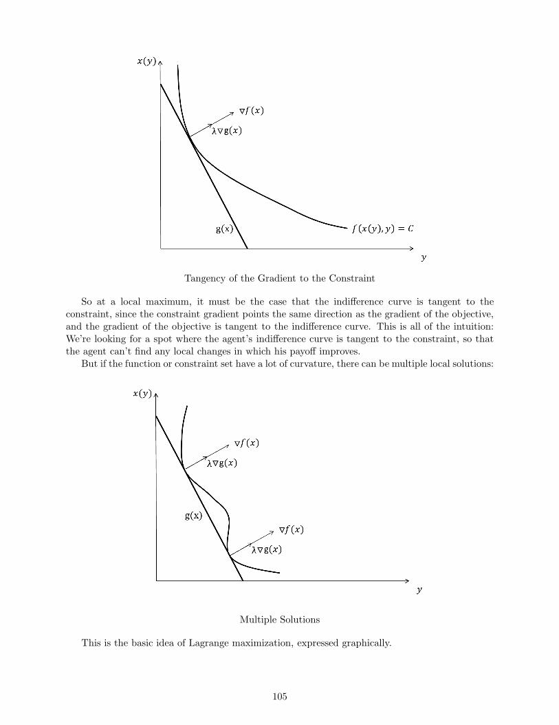
Tangency of the Gradient to the Constraint

So at a local maximum, it must be the case that the indifference curve is tangent to theconstraint, since the constraint gradient points the same direction as the gradient of the objective,and the gradient of the objective is tangent to the indifference curve. This is all of the intuition:We’re looking for a spot where the agent’s indifference curve is tangent to the constraint, so thatthe agent can’t find any local changes in which his payoff improves.

But if the function or constraint set have a lot of curvature, there can be multiple local solutions:

Multiple Solutions

This is the basic idea of Lagrange maximization, expressed graphically.

105

10.2.2 The Lagrange Multiplier

What is the interpretation of the Lagrange multiplier? Consider the problem of maximizing f(x)subject to a linear constraint w = p′x, p ≫ 0. You can think of w as an agent’s wealth, p asthe prices, and f(x) as their payoff from consuming a bundle x. The Lagrangean evaluated at theoptimum is:

L(x∗, λ∗) = f(x∗)− λ(p′x∗ − w)

But if we consider this instead as a function of w and differentiate, we get

V ′(w) = (∇f(x∗(w)) − λp)︸ ︷︷ ︸

First-order condition

∇wx∗(w) − ∂λ∗

∂w(p · x∗ − w)︸ ︷︷ ︸

=0

+λ∗(w)

So V ′(w) = λ∗(w), and the Lagrange multiplier gives the change in the optimized value of theobjective for a small relaxation of the constraint set. Economists often call it the shadow price ofw — how much the decision-maker would be willing to pay to relax the constraint slightly.

10.2.3 The Constraint Qualification

The constraint qualification can be confusing because it is a technical condition that has nothingto do with maximization. To make some sense of it (and generalize things a bit), consider thefollowing problem:

maxx

f(x)

subject to m = 1, 2, ...,M equality constraints, g1(x) = 0, g2(x) = 0, ..., gM (x) = 0. Let

g(x) =

g1(x)g2(x)...

gM (x)

The new Langrangean is given by

L(x, λ) = f(x)−M∑

m=1

λmgm(x) = f(x)− λ′g(x)

Theorem 10.2.3 (First-Order Necessary Conditions) If

1. x∗ is a local maximum of f(x) that satisfies the constraints g(x) = 0

2. the constraint gradients ∇g(x∗) 6= 0 (this is called the constraint qualification)

3. f(x) and g(x) are both differentiable at x∗

Then there exists a unique vector λ∗ such that the FONCs

∇xL(x∗, λ∗) = ∇f(x∗)− λ∗′∇g(x∗)

∇λL(x∗, λ∗) = −g(x∗) = 0

hold.

106

Now, the new FONCs are

∇f(x)− λ′∇g(x) = ∇f(x)−M∑

m=1

λm∇gm(x)

−g(x) = 0

The term

∇g(x) =

∂g1(x)

∂x1

∂g1(x)

∂x2. . .

∂g1(x)

∂xN∂g2(x)

∂x1

∂g2(x)

∂x2...

. . .∂gM (x)

∂x1

∂gM (x)

∂xN

is actually an M ×N matrix. Call this matrix G, just to clean things up a bit. Now our FONCsare

∇f(x) = λ′G

g(x) = 0

Remember that we are trying to solve for λ — that’s what Lagrange’s theorem guarantees — sowe need G to be invertible, so that

λ∗ = G−1∇f(x)

But if G fails to be invertible, we can’t solve for λ∗, and we can’t “finish the proof”.So the constraint qualification is just saying, “The matrix G is invertible,” nothing more.

Example Here’s an example where the constraint qualification fails with only one constraint:

max{x,y:y3−x2=0}

−y

The Lagrangean isL = −y − λ(y3 − x2)

with first-order necessary conditions−(y3 − x2) = 0

−1− λ3y2 = 0

λ2x = 0

The constraint y3 − x2 = 0 requires that both x and y be (weakly) positive. Since the objectiveis decreasing in y and non-responsive in x, the global maximum is at y∗ = x∗ = 0. But then thefirst-order necessary conditions are

0−10

6=

000

and cannot be satisfied.

So we have a simple situation where the Lagrange approach fails. The reason is that theconstraints have gradient

[∂g(0, 0)/∂x∂g(0, 0)/∂y

]

=

[00

]

so the constraint vanishes at the optimum. Then ∇L = ∇f + λ∇g cannot be solved if ∇f 6= 0 but∇g is. This is the basic idea of the constraint qualification.

107

10.3 Second-Order Sufficient Conditions

Just like unconstrained problems, there are second-order conditions, but they more complicated andrequire patience and practice to understand. There are two main differences from the unconstrainedproblem.

First, we need not consider all possible local changes in the choice variables x∗ to verify whethera particular critical point is a local maximum, but only those that do not violate the constraints.For example, if the function if f(x, y) = xy and the constraint is w = px + y, there are alwaysbetter allocations nearby any critical point, but most of them violate the constraint w = px + y.The set of changes (dx, dy) that leave the total expenditure unchanged satisfy pdx+ dy = 0, andthese are the only changes which we are really interested in.

Definition 10.3.1 Let (x∗, λ∗) be a critical point of the Lagrangian. The set of feasible localvariations is

Y = {y ∈ Rn : ∇g(x∗) · y = 0}

This is the set of vectors y local to x∗ for which all of the constraints are still satisfied, in the senseof the directional derivative, ∇g(x∗) · y = 0.

Second, the Hessian of L(x, λ) is not just the Hessian of f(x). Intuitively, I have suggested thatwe should think of equality constrained maximization of x subject to g(x) = 0 as unconstrainedmaximization of L(x, λ) in terms of (x, λ). This is reflected in the fact that the Hessian of L(x, λ)is the focus of the SOSCs, not the Hessian of f(x).

Theorem 10.3.2 (Second-Order Sufficient Conditions) Suppose (x∗, λ∗) is a critical pointof the Lagrangian (i.e., the constraint qualification and the FONCs ∇f(x∗) + λ∗′∇g(x∗) = 0 andg(x∗) = 0 are satisfied). Let ∇xxL(x∗, λ∗) be the Hessian of the Lagrangean function with respectto the choice variables only. Then

• If y′∇xxL(x∗, λ∗)y < 0 for all feasible local changes y, then x∗ is a local maximum of f

• If y′∇xxL(x∗, λ∗)y > 0 for all feasible local changes y, then x∗ is a local minimum of f

Since we are not solving an unconstrained maximization problem and the solution must lie onthe locus of points defined by g(x) = 0, it follows that we can imagine checking the local, second-order sufficient conditions only on the locus. Since we are using calculus, we restrict attention tofeasible local changes, and the consequence is that for all “small steps” y that do not violate theconstraint, the Lagrangian must have a negative definite Hessian in terms of x alone. This does notmean that the Hessian of the Lagrangian is negative definite, because the Lagrangian depends onx and λ. However, we would like a test that avoids dealing with the set of feasible local variationsdirectly, since that set appears difficult to solve for and manipulate.

Example IfL(x, y, λ) = f(x, y)− λ(ax+ by − c)

then the FONCS are−(ax+ by − c) = 0

fx(x∗, y∗)− λ∗a = 0

fy(x∗, y∗)− λ∗b = 0

Now, differentiating all the equations again in the order λ∗, x∗, and y∗ gives the matrix

∇xxL(x∗, y∗, λ∗) =

0 −a −b−a fxx(x

∗, y∗) fyx(x∗, y∗)

−b fxy(x∗, y∗) fyy(x

∗, y∗)

108

The above Hessian is called bordered, since the first column and first row are transposes of eachother, while the lower right-hand corner is the Hessian of the objective function.

For a single constraint g(x), the Hessian of the Lagrangean looks like this:

∇xxL(x∗, λ∗) =

[0 ∇xg(x

∗)′

∇xg(x∗) ∇xxf(x

∗) + λ∗∇xxg(x∗)

]

(10.1)

This is called the bordered Hessian.

Suppose you are maximizing f(x) subject to a single constraint, g(x) = 0 (you can find thegeneralization to any number of constraints in any math econ textbook). Then the determinant ofthe upper-left hand corner is trivially zero. The non-trivial leading principal minors of the borderedHessian are — for the case with a single constraint —

H3 =

0 −gx1(x∗) −gx2(x

∗)−gx1(x

∗) fx1x1(x∗)− λ∗gx1x1(x

∗) fx2x1(x∗)− λ∗gx2x1(x

∗)−gx2(x

∗) fx1x2(x∗)− λ∗gx1x2(x

∗) fx2x2(x∗)− λ∗gx2x2(x

∗)

H4 =

0 −gx1(x∗) −gx2(x

∗) −gx3(x∗)

−gx1(x∗) fx1x1(x

∗)− λ∗ − gx1x1(x∗) fx2x1(x

∗)− λ∗ − gx2x1(x∗) fx3x1(x

∗)− λ∗ − gx3x1(x∗)

−gx2(x∗) fx1x2(x

∗)− λ∗ − gx1x2(x∗) fx2x2(x

∗)− λ∗ − gx2x2(x∗) fx3x2(x

∗)− λ∗ − gx3x2(x∗)

−gx3(x∗) fx1x3(x

∗)− λ∗ − gx1x3(x∗) fx2x3(x

∗)− λ∗ − gx2x3(x∗) fx3x3(x

∗)− λ∗ − gx3x3(x∗)

...

Hk+1 =

0 −gx1(x∗) . . . −gxk

(x∗)−gx1(x

∗) fx1x1(x∗)− λ∗gx1x1(x

∗)...

. . .

−gxk(x∗) fxkxk

(x∗)− λ∗gxkxk(x∗)

So Hk+1 is the upper left-hand k + 1 × k + 1 principal minor of the full bordered Hessian. The“+1” term comes from the fact that we have an extra leading row and column that correspond tothe constraint.

An example makes this a bit clearer:

Example Letf(x1, x2, x3) = x1x2 + x2x3 + x1x3

subject tox1 + x2 + x3 = 3

Then the Lagrangean is

L = x1x2 + x2x3 + x1x3 − λ(x1 + x2 + x3 − 3)

This generates a system of first-order conditions:

∂L/∂λ∂L/∂x1∂L/∂x2∂L/∂x3

=

(3− x1 − x2 − x3)x2 + x3 − λx1 + x3 − λx2 + x1 − λ

The only critical point is x∗ = (1/3, 1/3, 1/3). The bordered Hessian at the critical point is

∇xxL(x∗, λ∗) =

0 −1 −1 −1−1 0 1 1−1 1 0 1−1 1 1 0

109

and the leading principal minors are

H3 =

0 −1 −1−1 0 −1−1 −1 0

and

H4 =

0 −1 −1 −1−1 0 1 1−1 1 0 1−1 1 1 0

It turns out that we can develop a test based on the bordered Hessian of the whole Lagrangian,including derivatives with respect to the multiplier, rather than focusing on the Hessian of theLagrangian restricted only to the choice variables.

Theorem 10.3.3 (Alternating Sign Test) • A critical point (x∗, λ∗) is a local maximum off(x) subject to the constraint g(x) = 0 if the determinants of all the principal minors of thebordered Hessian alternate in sign, starting with

detH3 > 0

• A critical point (x∗, λ∗) is a local minimum of f(x) subject to the constraint g(x) = 0 if thedeterminants of all the principal minors of the bordered Hessian are all negative, starting with

detH3 < 0

Returning to the example,

Example We need to decide whether the bordered Hessian is negative definite or not. Thenon-trivial leading principal minors of the bordered Hessian are

det(H3) = 2 > 0, det(H4) = −3 < 0

And the second-order condition is satisfied for any vector y′Hy.

Example Letf(x1, x2) = f1(x1) + f2(x2)

where f1(x1) and f2(x2) are increasing and f ′′1 (x), f

′′2 (x) < 0, and fi(0) = 0. There is a constraint

that C = x1 + x2. Then the Lagrangean is

L = f1(x1) + f2(x2)− λ(x1 + x2 − C)

This generates a system of first-order conditions

∂L/∂λ∂L/∂x1∂L/∂x2

=

−(x1 + x2 − C)f ′1(x1)− λf ′2(x2)− λ

with bordered Hessian

H(x, λ) =

0 −1 −1−1 f ′′

1 (x1) 0−1 0 f ′′

2 (x2)

110

Then the bordered Hessian’s non-trivial leading principal minors starting from H3 have determi-nants

det(H3) = −f ′′1 (x1)− f ′′

2 (x2) > 0

So the Lagrangian is negative definite, and an interior solution to the first-order conditions is asolution to the maximization problem.

Example Suppose a consumer is trying to maximize utility, with utility function u(x, y) = xαyβ

and budget constraint w = px+ y. Then we can write the Lagrangian as (why?)

L = α log(x) + β log(y)− λ(px+ y − w)

we get a system of first-order conditions

∂L/∂λ∂L/∂x∂L/∂y

=

w − px− yα/x− λpβ/y − λ

The Hessian of the Lagrangean is

0 −p −1

−p−α

(x∗)20

−1 0−β

(y∗)2

The determinants of the non-trivial leading principal minors of the bordered Hessian are

det

0 −p −1

−p−α

(x∗)20

−1 0−β

(y∗)2

= p(−p)

−β

(x∗)2− 1(−1)(−1)

−α

(x∗)2> 0

So the alternating sign test is satisfied.

This works because adding the border imposes the restriction that ∇g(x) = 0 on the test ofwhether the objective is negative definite or not. Consequently, when we use the alternating signtest, we are really asking, “Is the Hessian of the objective negative definite on Y ?” This requiresmore matrix algebra to show, but you can find the details in MWG or Debreu’s papers, for example.

10.4 Comparative Statics

Our system of first-order necessary conditions

∇xf(x∗)− λ∗∇xg(x

∗) = 0

−g(x∗) = 0

is a non-linear system of equations with endogenous variables (x∗, λ∗), just like any other wehave applied the IFT to. The only “new” part is that you have to keep in mind that λ∗ is anendogenous variable, so that it changes when we vary any exogenous variables. Second, the sign ofthe determinant of the Hessian is determined by whether we are looking at a maximum or minimum,and the number of equations.

111

For simplicity, consider a constrained maximization problem

maxx,y

f(x, y, t)

subject to a single equality constraint ax+ by− s = 0, where t and s are exogenous variables. Thisis simpler than assuming that g(x, s) = 0, since the second-order derivatives of the constraint areall zero. However, there are many economic problems of interest where the constraints are linear,and a general g(x, s) can be very complicated to work with. Then the Lagrangean is

L(x, y, λ) = f(x, y, t)− λ(ax+ by − s)

and the FONCs are−(ax∗ + by∗ − s) = 0

∇f(x∗, y∗, t)− λ∗∇g(x∗, y∗, s) = 0

Since we have two parameters — t shifts the objective function, s shifts the constraint — we canlook at two different comparative statics.

Example Let’s start with t: Totally differentiate the FONCs to get three equations

−(

a∂x∗

∂t+ b

∂y∗

∂t

)

= 0

ftx + fxx∂x∗

∂t+ fyx

∂y∗

∂t− ∂λ∗

∂ta = 0

fty + fxy∂x∗

∂t+ fyy

∂y∗

∂t− ∂λ∗

∂tb = 0

If we write this as a matrix equation,

0 −a −b−a fxx fxy−b fyx fyy

∂λ∗/∂t∂x∗/∂t∂y∗/∂t

=

0−ftx−fty

Which is just a regular “Ax = b”-type matrix equation. On the right-hand side, the borderedHessian appears; from the alternating sign test and the fact that x∗ is a local maximum, we candetermine the sign of its determinant. To some extent, we are finished, since all that remains isto solve the system. You can solve the system by hand by solving for each comparative static andreducing the number of equations, but that is a lot of work. It is simpler to use Cramer’s rule. Tosee how x∗ varies with t,

∂x∗

∂t=

det

0 0 −b−a −ftx fxy−b −fty fyy

detH3

which is∂x∗

∂t=

−b(afty(x∗, y∗, t)− bftx(x

∗, y∗, t)

detH3

Since (x∗, y∗) is a local maximum, detH3 > 0, and the sign of the comparative static is just thesign of the numerator.

Having done t, let’s do s:

112

Example Totally differentiate the system of FONCs to get

−(

a∂x∗

∂s+ b

∂y∗

∂s− 1

)

= 0

fxx∂x∗

∂s+ fyx

∂y∗

∂s− ∂λ∗

∂sa = 0

fxy∂x∗

∂s+ fyy

∂y∗

∂s− ∂λ∗

∂sb = 0

Writing this as a matrix equation yields

0 −a −b−a fxx fxy−b fyx fyy

∂λ∗/∂s∂x∗/∂s∂y∗/∂s

=

−100

Let’s focus on ∂y∗/∂s. Using Cramer’s rule,

∂y∗

∂s=

det

0 −a −1−a fxx 0−b fyx 0

detH3

∂y∗

∂s=

afyx + bfxxdetH3

An example with more economic content is:

Example Consider the consumer problem

L = α log(x) + β log(y)− λ(px+ y − w)

we get a system of first-order conditions

∂L/∂λ∂L/∂x∂L/∂y

=

w − px− yα/x− λpβ/y − λ

This is a system of non-linear equations, so there’s no problem differentiating it with respect to p,for instance, and using all the same steps as for the unconstrained firm. You need to remember,however, that λ∗(w, p, α, β) is now a function of parameters as well, so it is not a constant thatdrops out. Totally differentiating with respect to p gives

0 = −x− p∂x

∂p− ∂y

∂p

0 =−α

x2∂x

∂p− ∂λ

∂pp− λ

0 =−β

y2∂y

∂p− ∂λ

∂p

Solving the system the “long way” for ∂x/∂p gives

∂x

∂p= −

β

y∗2px∗ + λ∗

α

x∗2+

β

y∗2p2

< 0

Since the Lagrange multiplier λ∗ is positive, if p goes up, the consumer reduces his consumption ofx∗.

113

10.5 The Envelope Theorem

The last tool we need to generalize is the envelope theorem. Since a local maximum of the La-grangian satisfies

L(x∗, λ∗) = f(x∗)− λ∗′g(x∗) = f(x∗)

we can use it as our value function.As a start, suppose we are studying the consumer’s problem with utility function u(x, y) and

budget constraint w = px+ y. Then the Lagrangian at any critical point is

L(x∗, y∗, λ∗) = u(x∗, y∗)− λ∗(px∗ + y∗ − w)

Let’s consider it as a value function in terms of w,

V (w) = u(x∗(w), y∗(w)) − λ∗(w)(px∗(w) + y∗(w)− w)

Then

V ′(w) = uxx∗′(w) + uyy

∗′(w)︸ ︷︷ ︸

I

−λ∗(w)px∗′(w) − λ∗(w)y∗′(w)︸ ︷︷ ︸

II

−λ∗′(w)(px∗(w) + y∗(w) −w)︸ ︷︷ ︸

III

+λ∗(w)︸ ︷︷ ︸

IV

There are a bunch of terms that each represent a different consequence of giving the agent morewealth. First, the agent re-optimizes and the value of the objective function changes (I). Second,this has an impact on the constraint, and its implicit cost changes (II). Third, since the constrainthas been relaxed, the Lagrange multiplier changes, again changing the implicit cost (III). Fourth,there is the direct effect on the objective of increasing w (IV).

Re-arranging, however, gives

V ′(w) = (ux − λ∗(w)p)x∗′(w) + (uy − λ∗(w))y∗′(w)︸ ︷︷ ︸

FONCs

−λ∗′(w) (px∗(w) + y∗(w) −w)︸ ︷︷ ︸

Constraint

+λ∗(w)

so that the FONCs are zero, and since the constraint is satisfied, that term also equals zero, leavingjust the direct effect,

V ′(w) = λ∗(w)

or

V ′(w) =∂L(x∗(w), y∗(w), λ∗(w), w)

∂w=

dL(x∗(w), y∗(w), λ∗(w), w)

dw

So as before, we can simply take the partial derivative of the Lagrangean to see how an agent’spayoff changes with respect to a parameter, rather than working out all the comparative staticsthrough the implicit function theorem.

Theorem 10.5.1 (Envelope Theorem) Consider the constrained maximization problem

maxx

f(x, t)

subject to g(x, s) = 0. Let x∗(t, s), λ∗(t, s) be a critical point of the Lagrangean. Define

V (t, s) = L(x∗(t, s), λ∗(t, s), t, s) = f(x∗(t, s), t) + λ∗(t, s)g(x∗(t, s), s)

Then∂V (t, s)

∂t=

∂f(x∗(t, s), t)

∂t

and∂V (t, s)

∂s=

∂g(x∗(t, s), s)

∂s

114

In words, the envelope theorem implies that a change in the agent’s payoff with respect to anexogenous variable is the partial derivative of the non-optimized Lagranian evaluated at the optimaldecision x∗(t, s).

Example Suppose a firm has production function F (K,L, t) where K is capital, L is labor, andt is technology. The price of the firm’s good is p. Then the we can write the profit maximizationproblem as a constrained maximization problem as

π(t) = maxq,K,L

pq − rK − wL

subject to q = F (K,L, t). The Lagrangean then is

L(q,K,L, λp) = pq − rK − wL− λp(q − F (K,L, t))

And — without any actual work —

π′(t) = λ∗pFt(K

∗, L∗, t)

Similarly, the cost minimization problem is

C(q, t) = minK,L

rK + wL

subject to F (K,L, t) ≥ q. The Lagrangean then is

L(K,L, λ) = −rK − wL+ λc(F (K,L, t) − q)

AndCt(q, t) = λ∗

cFt(K∗, L∗, t)

So be careful: The envelope theorem takes the derivative of the Lagrangean, then evaluates itat the optimal choice to obtain the derivative of the value function.

Exercises

1. Suppose we take a strictly increasing transformation of the objective function and leave theconstraints unchanged. Is a solution of the transformed problem a solution of the original problem?Suppose we have constraints g(x) = c and take a strictly increasing transformation of both sides.Is a solution of the transformed problem a solution of the original problem?

2. Consider the maximization problem

maxx1,x2

x1 + x2

subject tox21 + x22 = 2

Sketch the constraint set and contour lines of the objective function. Find all critical points of theLagrangian. Verify whether each critical point is a local maximum or a local minimum. Find theglobal maximum.

3. Consider the maximization problem

maxx,y

xy

115

subject toa

2x2 +

b

2y2 = r

Sketch the constraint set and contour lines of the objective function. Find all critical points of theLagrangian. Verify whether each critical point is a local maximum or a local minimum. Find theglobal maximum. How does the value of the objective vary with r? a? How does x∗ respond to achange in r; show this using the closed-form solutions and the IFT.

4. Solve the problemmaxx,y,z

2x− 2y + z

subject to x2 + y2 + z2 = 9.

5. Solve the following two dimensional maximization problems subject to the linear constraintw = p1x1 + p2x2, p1, p2 > 0. Then compute the change in x1 with respect to p2, and a change inx1 with respect to w. Assume α1 > α2 > 0. For i and ii, when do the SOSCs hold?

i. Cobb-Douglasf(x) = xα1

1 xα22

ii. Stone-Gearyf(x) = (x1 − γ1)

α1(x2 − γ2)α2

iii. Constant Elasticity of Substitution(

α1x1/ρ1 + α2x

1ρ2

)ρ

iv. Leontiefmin{α1x1, α2x2}

6. An agent receives income w1 in period one and no income in the second period. He consumesc1 in the first period and c2 in the second. He can save in the first period, s, and receives back Rsin the second period. His utility function is

u(c1, c2) = log(c1) + δ log(c2)

where R > 1 and 0 < δ < 1. (i) Write this down as a constrained maximization problem. (ii)Find first-order necessary conditions for optimality and check the SOSCs. What does the Lagrangemultiplier represent in this problem? (iii) Compute the change in c2 with respect to R and δ. (iv)How does the agent’s payoff change if R goes up? δ?

7. For utility functionu(x1, x2) = (x1 − γ1)x

α2

and budget constraint w = p1x1 + p2x2, compute the utility-maximizing bundle. You should getclosed-form solutions. Now compute ∂x∗1/∂p2 using the closed-form solution as well as the implicitfunction theorem from the system of FONCs. Repeat with ∂x∗2/∂p1. How does the agent’s payoffvary in γ1? w? p2?

8. Generalize and proof the envelope theorem in the case where f(x, t) and g(x, t) both dependon the same parameter, t. Construct an economically relevant problem in which this occurs, anduse the implicit function theorem to show how x∗(t) varies in t when both the constraint andobjective are varying at the same time.

9. Suppose you are trying to maximize f(x). Show that if the constraint is linear, so thatp · x = w, you can always rewrite the constraint as

xN =

∑N−1i=1 pixipN

116

and substitute this into the objective, turning the problem into an unconstrained maximizationproblem. Why do we need Lagrange maximization then?

10. Suppose you have a maximization problem

maxx

f(x)

subject to g(x, t) = 0. Show how to use the implicit function theorem to derive comparative staticswith respect to t. Explain briefly what the bordered Hessian looks like, and how it differs from theexamples in the text.

117

Chapter 11

Inequality-Constrained MaximizationProblems

Many problems — particularly in macroeconomics — don’t involve strict equality constraints, butinvolve inequality constraints. For example, a household might be making a savings/consumptiondecision, subject to the constraint that savings can never become negative — this is called aborrowing constraint. As a result, many households will not have to worry about this, as long asthey maintain positive savings in all periods. A simple version is:

Example Consider a household with utility function

u(c1) + δu(c2)

The household gets income y1 in period one and y2 in period two, with y2 > y1. The household wouldpotentially like to borrow money today to smooth consumption, but faces a financial constraintthat it can borrow an amount B only up to R < y2. Then we have the constraints

c1 = y1 +B

c2 = y2 −B

B ≤ R

Substituting the first two constraints into the objective yields

maxB

u(y1 +B) + δu(y2 −B)

subject to B ≤ y2.Now, sometimes the constraint will be irrelevant, or

u′(y1 +B∗) = δu′(y2 −B∗)

and B∗ < R, and the constraint is “slack,” or “inactive.” Other times, however, B∗ > R, and theconstraint becomes “binding” or “active”. Then B′ = R, and we have two potential solutions, andthe one selected depends on the parameters of the problem.

The simple borrowing problem illustrates the general issues: Having inequality constraints cre-ates the possibility that for different values of the parameters, different collections of the constraintsare binding. The maximization theory developed here is designed to deal with these shifting setsof constraints.

118

Definition 11.0.2 Let f(x) be the objective function. Suppose that the choice of x is subjectto m = 1, 2, ...,M equality constraints, gm(x) = 0, and k = 1, 2, ...,K inequality constraints,hk(x) ≤ 0. Then the inequality-constrained maximization problem is

maxx

f(x)

such that for m = 1, 2, ...,M and k = 1, 2, ...,K,

gm(x) = 0

hk(x) ≤ 0

Note that we can brute force solve this problem as follows: Since there are K inequality con-straints, there are 2K ways to pick a subset of the inequality constraints. For each subset, we canmake the chosen inequality constraints into equality constraints, and solve the resulting equalityconstrained maximization problem (which we already know how to do). Each of these sub-problemsmight generate no candidates, or many, and some of the candidates may conflict with some of theconstraints we are ignoring. Once we compile a list of all the solutions that are actually feasible,then the global maximum must be on the list somewhere. Then we can simply compare the payoffsfrom our 2K sets of candidate solutions, and pick the best.

Example Suppose an agent is trying to maximize f(x, y) = ax + by, a, b > 0, subject to theconstraints x ≥ 0, y ≥ 0, and c ≥ px+ qy.

Since ∇f = (a, b) ≫ 0, it is immediate that the constraint c ≥ px+qy will bind with an equality.For if c > px+ qy, we can always increase x or y a little bit, thus improving the objective function’svalue as well as not violating the constraint. This is feasible and better than any proposed solutionwith c > px+ qy, so we must have c = px+ qy.

Then we have three cases remaining:

1. The constraint x ≥ 0 binds and x = 0, but y > 0

2. The constraint y ≥ 0 binds and y = 0, but x > 0

3. The constraints x, y ≥ 0 are both slack, and x, y > 0

We then solve case-by-case:

1. If y = 0, then the constraint implies x = c/p, giving a value of ac/p

2. If x = 0, then the constraint implies y = c/q, giving a value of bc/q

3. If x, y > 0, then we solve the constrained problem using a Lagrangean,

L(x, y, λ) = ax+ by − λ(px+ qy − c)

with FONCsa− λp = 0

b− λq = 0

and−(px+ qy − c) = 0

This has a solution only if a/b = p/q, in which case any x and y that satisfy the constraintsare a solution, since the objective is equivalent to (a/b)x+ y and the constraint is equivalentto (p/q)x + y, from which you can easily see that the indifference curves and constraint setare exactly parallel, so that any px∗ + qy∗ = c with x∗, y∗ > 0 is a solution.

119

So we have two candidate solutions with either x or y equal to zero, and a continuum of solutionswhen the objective and constraint are parallel.

As happened in the previous problem, we differentiate between two kinds of solutions:

Definition 11.0.3 A point x∗ that is a local maximizer of f(x) subject to gm(x) = 0 for all mand hk(x) ≤ 0 for all k is a corner solution if hk(x

∗) = 0 for some k, and an interior solution ifhk(x

∗) < 0 for all k.

A corner solution is one like x∗ = c/p and y∗ = 0, while an interior solution corresponds to thethird case from the previous example, where the constraint c = px+ qy binds.

This example suggests we don’t really need a new maximization theory, but either a lot ofpaper or a powerful computer. However, just as Lagrange multipliers can be theoretically useful,the multipliers we’ll attach to the inequality constraints can be theoretically useful. In fact, theframework we’ll develop is mostly just a systematic way of doing the brute force approach describedin the previous paragraph.

11.1 First-Order Necessary Conditions

For simplicity, we’ll work with one equality constraint g(x) = 0 and k = 1, ...,K inequality con-straints, hk(x) ≤ 0.

As before, we form the Lagrangean, putting a Lagrange multiplier λ on the equality constraint,and µ = (µ1, µ2, ..., µK) Kuhn-Tucker multipliers on the inequality constraints:

L(x, λ, µ) = f(x)− λg(x) −∑

k

µkhk(x) = f(x)− λg(x)− µ′h(x)

But now we have a dilemma, because some constraints may be binding at the solution while othersare not. Moreover, there may be many solutions that correspond to different binding constraintsets. How are we supposed to know which bind and which don’t? We proceed by making the setof FONCs larger to include complementary slackness conditions.

Theorem 11.1.1 (Kuhn-Tucker First-Order Necessary Conditions) Suppose that

1. Suppose x∗ is a local maximum of f(x) subject to the constraints g(x) = 0 and hk(x) ≤ 0 forall k.

2. Let E = {1, 2, ..., ℓ} be the set of inequality constraints that binding at x∗, so that hj(x∗) = 0

for all j ∈ E and hj(x∗) < 0 for all j /∈ E. Suppose that the matrix formed by the

gradient of the equality constraint, ∇g(x∗), and the binding inequality constraints in E,∇h1(x

∗),∇h2(x∗), ...,∇hℓ(x

∗), is non-singular (this is the constraint qualification).

3. The objective function, equality constraint, and inequality constraints are all differentiable atx∗

Then, there exist unique vectors λ∗ and µ∗ of multipliers so that

• the FONCs∇f(x∗)− λ∗∇g(x∗)−

∑

j

µ∗jhj(x

∗) = 0

−g(x∗) = 0

120

• and the complementary slackness conditions

µ∗jhj(x

∗) = 0

for all k = 1, ...,K

are satisfied.

So, we always have the issue of the constraint qualification lurking in the background of aconstrained maximization problem, so set that aside. The rest of the theorem says that if x∗

is a local maximum subject to the equality constraint and inequality constraints, some will beactive/binding and some will be inactive/slack. If we treat the active/binding constraints as regularequality constraints, then µ∗

j ≥ 0 for each binding constraint, but each slack constraint will satisfyhj(x

∗) < 0, so µ∗j = 0 — these are the complementary slackness conditions. (Note that it is not

obvious right now that µ∗j ≥ 0, but this is shown later.)

Example Suppose a consumer’s utility function is u(x, y), and he faces constraints x ≥ 0, y ≥ 0and w = px+ y. Suppose that ∇u(x, y) ≥ 0, so that the consumer’s utility is weakly increasing inthe amount of each good.

Then we can form the Lagrangian

L(x, y, µ) = u(x, y)− µxx− µyy − λ(px+ y − w)

The FONCs areux(x

∗, y∗)− µ∗x − λ∗p = 0

uy(x∗, y∗)− µ∗

y − λ∗ = 0

−(px∗ + y∗ − w) = 0

and the complementary slackness conditions are

µ∗xx

∗ = 0

µ∗yy

∗ = 0

Now we hypothetically have 22 = 4 cases:

1. µ∗x, µ

∗y ≥ 0 (which will imply x∗ = 0, y∗ = 0 by the complementary slackness conditions)

2. µ∗x = 0,µ∗

y ≥ 0 (which will imply x∗ > 0, y∗ = 0 by the complementary slackness conditions)

3. µ∗x ≥ 0,µ∗

y = 0 (which will imply x∗ = 0, y∗ > 0 by the complementary slackness conditions)

4. µ∗x, µ

∗y = 0 (which will imply x∗, y∗ > 0 by the complementary slackness conditions)

We now solve the FONCs case-by-case:

1. In the first case, µ∗x, µ

∗y ≥ 0, we look at the corresponding complementary slackness conditions

µ∗xx

∗ = 0

µ∗yy

∗ = 0

For these to hold, it must be the case that x∗ = 0 and y∗ = 0. Substituting these into theFONCs yields

ux(0, 0) − µ∗x − λ∗p = 0

uy(0, 0) − µ∗y − λ∗ = 0

w = 0

which yields a contradiction, since w = 6= 0. This case provides no candidate solutions.

121

2. In the second case, µ∗x = 0,µ∗

y ≥ 0, we look at the complementary slackness conditions

µ∗xx

∗ = 0

µ∗yy

∗ = 0

For these to hold, y∗ must be zero. Substituting this into the FONCs yields

ux(x∗, 0) − λ∗p = 0

uy(x∗, 0) − µ∗

y − λ∗ = 0

−(px∗ − w) = 0

from which we get x∗ = w/p from the final equation. This case gives a candidate solutionx∗ = w/p and y∗ = 0.

3. In the third case, µ∗x 6= 0,µ∗

y = 0, we look at the complementary slackness conditions

µ∗xx

∗ = 0

µ∗yy

∗ = 0

For these to hold, we must have x∗ = 0. Substituting this into the FONCs yields

ux(0, y∗)− µ∗

x − λ∗p = 0

uy(0, y∗)− λ∗ = 0

−(y∗ − w) = 0

from which we get y∗ = w from the final equation. This case gives a candidate solution x∗ = 0and y∗ = w.

4. In the last case, µ∗x, µ

∗y = 0, the complementary slackness conditions are satisfied automati-

cally. Substituting this into the FONCS yields

ux(x∗, y∗)− λ∗p = 0

uy(x∗, y∗)− λ∗ = 0

−(px∗ + y∗ − w) = 0

which gives an interior solution x∗, y∗ > 0.

So the KT conditions produce three candidate solutions: All x and no y, all y and no x, and someof each. Which solution is selected will depend on whether ∇u(x, y) is strictly greater than zero oronly weakly greater than zero in each good.

The complementary slackness conditions work as follows: Suppose we have an inequality con-straint x ≤ 0. Then the complementary slackness condition is that µ∗

xx∗ = 0, where µ∗

x is theKuhn-Tucker multiplier associated with the constraint x ≤ 0. Then if µ∗

x ≥ 0, it must be thecase that x∗ = 0 for the complementary slackness condition to hold; if µ∗

x = 0, then x∗ can takeany value. This is how KT theory systematically works through all the possibilities of binding con-straints: if the KT multiplier is non-zero, the constraint must be binding, while if the KT multiplieris zero, it is slack.

122

Example Consider maximizing f(x, y) = xαyβ subject to the inequality constraints

y + 2x ≥ 6

x+ 2y ≥ 6

x ≥ 0

y ≥ 0

Then there are four inequality constraints. The set of points satisfying all four is not empty (graphit to check). However, the first two constraints only bind at the same time when x = y = 2;otherwise either the first is binding or the second but not both. This means that the Lagrangean isnot the right tool, because you could only satisfy both equations as equality constraints at the pointx = y = 2, which may not be a solution. You could set up a series of problems where you treatthe constraints as binding or non-binding, and solve the 24 resulting maximization problems thatcome from considering each subset of constraints separately, but this is exactly what Kuhn-Tuckerdoes for you, in a systematic way. The Lagrangean is

L = α log(x) + β log(y)− µ1(y + 2x− 6)− µ2(x+ 2y − 6)− µ3x− µ4y

The first-order necessary conditions are

[∂L/∂x∂L/∂y

]

=

α

x− 2µ1 − µ2 − µ3

β

y− µ1 − 2µ2 − µ4

The complementary slackness conditions are

µ1(y + 2x− 6) = 0µ2(x+ 2y − 6) = 0

µ3x = 0µ4y = 0

We now proceed by picking combinations of multipliers, and setting µj ≥ 0 if hj(x∗, y∗) = 0, and

µj = 0 if hj(x∗, y∗) > 0. This is what the “complementary” part of complementary slackness

means.First, note that the gradient is strictly increasing, so that if x = 0 or y = 0 at the optimium, it

occurs at an extreme point of the set. So if x = 0 (µ3 ≥ 0), then y must be as large as possible,and if y = 0 (µ4 ≥ 0), x must be as large as possible. Second, note that if 6 = y + 2x is binding(µ1 ≥ 0), then 6 = x+ 2y is slack (µ2 = 0), and vice versa.

So we really have five possibilities:

1. x = y = 2 and both µ1, µ2 ≥ 0 and µ3, µ4 = 0

2. x, y > 0 and µ1 ≥ 0, µ2, µ3, µ4 = 0

3. x, y > 0 and µ2 ≥ 0, µ1, µ3, µ4 = 0

4. x > 0 and y = 0, and µ1 ≥ 0, µ2, µ3, µ4 = 0

5. y > 0 and x = 0, and µ2 ≥ 0, µ1, µ3, µ4 = 0

For each case, we find the set of critical points that satisfy the resulting first-order conditions:

1. The unique critical point is x = y = 2.

123

2. If x, y > 0 and µ1 ≥ 0, the binding constraint is that y + 2x = 6. The first-order necessaryconditions become [

α/x − 2µ1

β/y − µ1

]

=

[00

]

This implies (why?) αy = 2βx. With the constraint, this implies

x∗ =3α

α+ β, y∗ =

6β

α+ β

3. If x, y > 0 and µ2 ≥ 0, the binding constraint is that 2y + x = 6. The first-order necessaryconditions become [

α/x− µ2

β/y − 2µ2

]

=

[00

]

Using the conditions and constraint gives

x∗ =6α

α+ β, y∗ =

3β

α+ β

4. If x > 0 and y∗ = 0, and µ1 ≥ 0, then the constraint 2x+ y = 6 binds, and x∗ = 3.

5. If y > 0 and x∗ = 0, and µ2 ≥ 0, then the constraint x+ 2y = 6 binds, and y∗ = 3.

So we have a candidate list of five potential solutions:

2 , 2

6α

α+ β,

3β

α+ β

3α

α+ β,

6β

α+ β3 , 0

0 , 3

To figure out which is the global maximum, you generally need to plug these back into theobjective and determine which point achieves the highest value. This will depend on the value ofα and β.

Example Suppose an agent is trying to solve an optimal portfolio problem, where two assets, xand y are available. Asset x has mean mx and variance vx, while asset y has mean my and variancevy. The covariance of x and y is vxy. He has wealth w, shares of x cost p, and shares of y cost 1, sohis budget constraint is w = xmx + ymy, but x ≥ 0 and y ≥ 0, so he cannot short. The objectivefunction is the mean minus the variance of the portfolio,

xmx + ymy − (x2vx + ym∗y − 2xyvxy)

Then the Lagrangean is

L = xmx + ymy − (x2vx + ym∗y − 2vxy)− λ(w − px− y)− µxx− µyy

The FONCs aremx − (2x∗vx − 2y∗vxy)− λp− µx = 0

my − (2y∗vy − 2x∗vxy)− λ− µy = 0

−(w − px∗ − y∗) = 0

124

and the complementary slackness conditions are

µ∗xx

∗ = 0

µ∗yy

∗ = 0

Then there are 22 = 4 cases:

1. µ∗x = mu∗y = 0, placing no restrictions on x∗ and y∗, by the complementary slackness condi-

tions

2. µ∗x = 0 and µ∗

y ≥ 0, so that y∗ = 0, by the complementary slackness conditions

3. µ∗x ≥ 0 and µ∗

y = 0, so that x∗ = 0, by the complementary slackness conditions

4. µ∗x ≥ 0 and µ∗

y ≥ 0, so that x∗ = y∗ = 0, by the complementary slackness conditions

We solve case by case:

1. If µ∗x = µ∗

y = 0, then the FONCs are

mx − (2x∗vx − 2y∗vxy)− λ∗p = 0

my − (2y∗vy − 2x∗vxy)− λ∗ = 0

−(w − px∗ − y∗) = 0

which is a quadratic programming problem and can be solved by matrix methods. In partic-ular,

y∗ =w(vx + pvxy)− p

2(mx − pmy)

p(2vxy + vy) + vx

2. If µ∗x = 0 and µ∗

y ≥ 0, then the FONCs are

mx − (2x∗vx)− λ∗p = 0

my − (−2x∗vxy)− λ∗ − µ∗y = 0

−(w − px∗) = 0

And the last equation gives a candidate solution x∗ = w/p and y∗ = 0.

3. This case is similar to the previous one, with y∗ = w/p and x∗ = 0.

So the portfolio optimization problem produces three candidate solutions. Our candidate solu-tion with x∗ and y∗ both positive requires

w(vx + pvxy)−p

2(mx − pmy) > 0

If p = 1, this reduces to

w >mx −my

2(vx + vxy)

so that the difference in means can’t be too large (mx−my) or the agent will prefer to purchase allx. If vx or vxy is large, however, this makes the agent prefer to diversify, even if mx > my. The KTconditions allow us to pick out the various solutions and compare them, even for large numbers ofassets (since this is just a quadratic programming problem).

125

11.1.1 The sign of the KT multipliers

We haven’t yet shown that µj ≥ 0. To do this, consider relaxing the first inequality constraint:

h1(x) ≤ ε

where ε is a relaxation parameter that makes the constraint easier to satisfy. The Lagrangian fora problem with one equality constraint and J inequality constraints becomes

L = f(x)− λg(x)− µ1(h1(x)− ε)−J∑

j=2

µjhj(x)

Let V (ε) be the value function in terms of ε. If we have relaxed the constraint, the agent’s choiceset is larger, and he must be better off, so that V ′(ε) ≥ 0. But by the envelope theorem,

V ′(ε) =∂L(x∗, λ∗, µ∗)

∂ε= µ∗

1 ≥ 0

So the KT multipliers must be weakly positive, as long as your constraints are always written ashj(x) ≤ 0.

11.2 Second-Order Sufficient Conditions and the IFT

Some good news: Since KTmaximization is essentially the same as Lagrange maximization once youhave fixed the set of binding constraints, the SOSCs and implicit function theorem for an inequality-constrained problem are to those in an equality-constrained maximization problem where the setof binding constraints are equality constraints, and the slack constraints are completely ignored.

Remember: KT is just a formal way of working through the process of testing all the possiblecombinations of binding constraints. So for a particular set of binding constraints, the problemis equivalent to an equality constrained problem where these are the only constraints. To checkwhether a critical point is a local maximum or compute comparative statics, we use exactly thesame approach as an equality constrained problem.

The envelope theorem is similar, but you have to be careful. In an inequality constrainedproblem there are potentially many local solutions for some values of the exogenous variables. Butthe envelope theorem is computed from the maximum of all of them, and as you vary the exogenousvariables, you have to be careful that you don’t drift into another solution’s territory. Locally, thereis not much to worry about, since you are almost never on such a boundary (in the sense of Lebesguemeasure zero). But suppose you want to plot the maximized value of the objective function for anagent facing a savings behavior for a variety of interest rates where there is a borrowing constraintthat binds for some values of the interest rate but not for others. However, this upper envelopeover all maximization solutions is continuous, at least (but not necessary differentiable at “kinks”where the regime switches):

Theorem 11.2.1 (Theorem of the Maximum) Consider maximizing f(x, c) over x, where thechoice set defined by the equality and inequality constraints is compact and potentially depends onc. Then f(x∗(c), c) is a continuous function in c.

The theorem of the maximum is a kind of generalization of the envelope theorem that says,“While V (c) may not be differentiable because of the kinks where the set of binding constraintsshifts, the value functions will always be at least continuous in a parameter c.”

126

Exercises

1. Suppose an agent has the following utility function:

u(x1, x2) =√x1 +

√x2

and faces a linear constraint1 = px1 + x2

and non-negativity constraints x1 ≥ 0, x2 ≥ 0.i. Verify the objective function is concave in (x1, x2). ii. Graph the budget set for various pricesp, and some of the upper contour sets. iii. Solve the agent’s optimization problem for all p > 0.Check the second-order conditions are satisfied at the optimum. iv. Sketch the set of maximizers asa function of p, x1(p). v. Solve the agent’s problem when u(x1, x2) =

√x1+

√x2 + 1. Is it possible

to get corner solutions in this case? Explain the difference between the old objective function andthe new one.

2. Suppose a firm hires capital K and labor L to produce output using technology q = F (K,L),with∇F (K,L) ≥ 0. The price of capital is r and the price of labor is w. Solve the cost minimizationproblem

minK,L

rK + wL

subject to F (K,L) ≥ q, K ≥ 0 and L ≥ 0. Check the SOSCs or otherwise prove that your solutionsare local maxima subject to the constraints. How does (K∗, L∗) vary in r and q at each solution?How does the firm’s cost function vary in q?

3. Warning: This question is better approached by thinking without a Lagrangean than tryingto use KT theory. A manager has two factories at his disposal, a and b. The cost function forfactory a is Ca(qa) where Ca(0) = 0 and Ca(qa) is increasing, differentiable, and convex. The costfunction for factory b is

Cb(qb) =

{

0 if qb = 0

cbqb + F if qb > 0

i. Is factory b’s cost function convex? Briefly explain the economic intuition of the propertyCb(0) = 0 but limqb↓0 Cb(qb) = F . ii. Solve for the cost-minimizing production plan (qa, qb) thatachieves q units of output, qa + qb = q, qa ≥ 0, qb ≥ 0. Is the cost function C∗(q) continuous?Convex? Differentiable? iii. Let p be the price of the good. If the firm’s profit function isπ(q) = pq − C∗(q), what is the set of maximizers of π(q)?

4. Suppose an agent has the following utility function:

u(x1, x2) =

{ √x1x2 , x2 > x1

x1 + x22

, x2 ≤ x1

and faces a linear constraint1 = px1 + x2

and non-negativity constraints x1 ≥ 0, x2 ≥ 0. (i.) Verify that these preferences are continuousbut non-differentiable along the ray x1 = x2. (ii.) Graph the budget set for various prices p, andsome of the upper contour sets. (iii.) Solve the agent’s optimization problem for all p > 0. (iv.)Sketch the set of maximizers as a function/correspondence of p, x1(p).

5. Suppose an agent gets utility from consumption, c ≥ 0, and leisure, ℓ ≥ 0. He has one unitof time, which can also be spent working, h ≥ 0. From working, he gets a wage of w per hour, andhis utility function is

u(c, ℓ)

127

However, he faces taxes, which take the form

t(wh) =

{0 , wh < t0

τwh ,wh ≥ t0

Therefore, his income is wh, consumption costs pc, and he is taxed based on whether his wage isabove or below a certain threshold, linearly at rate τ . i. Sketch the agent’s budget set. Is it a convexset? ii. Formulate a maximization problem and characterize any first-order necessary conditionsor complementary slackness conditions. iii. Characterize the agent’s behavior as a function of wand t0. What implications does this model have for the design of tax codes? iv. If the tax tookthe form

t(wh) =

{0 , wh < t0τ , wh ≥ t0

sketch the agent’s budget set. Is it convex? What implications does the geometry of this budgetset have for consumer behavior?

6. A consumer has wealth w, and access to a riskless asset with return R > 1, and a risky assetwith return r ∼ N(r, σ2). He places φ1 of his wealth into the riskless asset, and φ2 of his wealthinto the risky asset:

w = φ1 + φ2

and he maximizes the mean-less-the-variance of his returns:

U(φ1, φ2) = φ1R+ φ2r −γ

2φ22(σ

2 + r2)

(i) Find conditions on λ,R, r∗, σ2 so the agent holds some of both the risky and riskless assets, andsolve for the optimal portfolio weights, (φ∗

1, φ∗2). (ii) How do the optimal portfolio weights vary with

r∗, σ2 and R? (iii) How does his payoff vary with w and R when he uses the optimal portfolio?

128

Chapter 12

Concavity and Quasi-Concavity

Checking second-order sufficient conditions for equality- and inequality-constrained maximizationproblems is often outrageously painful. It is time-consuming and error-prone, and pain increasesexponentially in the number of choice variables.

For this reason, it would be very helpful to know when the second-order sufficient conditionsfor multi-dimensional maximization problems are automatically satisfied.

There are two classes of function that are useful for maximization: Concave and Quasi-concave.(The corresponding classes for minimization are Convex and Quasi-convex.)

In the one-dimensional case, strict concavity meant that f ′′(x) < 0 for all x. In the multi-dimensional case, strictly concavity will similarly mean that y′∇xxf(x)y < 0 for all x and y, and itfollows that the second-order conditions will be satisfied. This is the best case.

However, recall that if x∗ is a local maximum of f(x), then for any strictly increasing functiong(), x∗ is also a maximum of g(f(x)). This is nice, because it means that the “units” of f(x) areirrelevant to the set of maximizers. But concavity and convexity are not preserved under monotonetransformations. For example, log(x) is one of our prototype concave functions. But if we take thestrictly increasing transformation g(y) = (ey)2, we get

g(log(x)) = x2

which is a convex function.This has the potential to cause problems for us as economists, because we want the set of

maximizers to be independent of how we describe f(x) up to increasing transformations (that letsus claim that we don’t need “utils” or cardinal utility to measure people’s preferences, we can justobserve how they behave). We want our theories to be based on ordinal utility, meaning that thenumbers provided by a utility function are meaningless in themselves, and only serve to verifywhether one option is better than another.

This is where quasi-concavity comes in. It is a property similar to concavity that is preservedunder monotone transformations, and has the same convenient theorems built in.

12.1 Some Geometry of Convex Sets

For analyzing maximization problems, it is helpful to consider the behavior of the “better than”sets:

Definition 12.1.1 The upper contour sets of a function are the sets

UC(a) = {x : f(x) ≥ a}

Now, we need to be careful about the difference between convex sets and convex functions,since we’re about to use both words side by side quite a bit.

129

Definition 12.1.2 A set S is convex if, for any x′ and x′′ in S and any λ ∈ [0, 1], the point

xλ = λx′ + (1− λ)x′′

is also in S. The interior of a convex set S,∫(S), are all the points x for which there is a ball

Bδ(x) ⊂ S. If any convex combination is in the interior of S, then S is a strictly convex set.

Convexity

Convex sets are well behaved since you can never drift outside the set along a chord betweentwo points. Geometrically, if your upper contour sets are convex and the constraint set is strictlyconvex, then we should be able to “separate” them, like this:

130

Separation of Constraint and Upper-contour Sets

This would mean there is a unique maximizer, since there is a unique point of tangency betweenthe indifference curves and the constraint set.

Why? If we pick a point x0 on an indifference curve and some point x1 better than x0, all ofthe options along the path from x0 to x1 are better than x0. We might express this more formallyby saying that for λ ∈ [0, 1], the options xλ = λx1 + (1 − λ)x0 are all better than x0, or that theupper contour sets are convex sets. This is a key geometric feature of well-behaved constrainedmaximization problems.

12.2 Concave Programming

Concave functions are the best-case scenario for optimization, since they imply that first-ordernecessary conditions are sufficient for a critical point to be a global maximum (this makes checkingsecond-order sufficient conditions unnecessary, and life is much easier).

Definition 12.2.1 A function f(x) is concave if for all x′ and x′′ and all λ ∈ [0, 1],

f(λx′ + (1− λ)x′′) ≥ λf(x′) + (1 − λ)f(x′′)

It is strictly concave if the equality is strict for all λ ∈ (0, 1).

131

Concave functions

This is a natural property in economics: Agents often prefer variety — consuming the bundleλx′+(1−λ)x′′ — to consuming either of two “extreme” bundles. For example, which sounds better:Five apples and five oranges, or ten apples with probability 1/2 and ten oranges with probability1/2? If you say, “Five apples and five oranges”, you have concave preferences.

However, there are many, equivalent ways to characterize a concave function:

Definition 12.2.2 The following are equivalent:

• f(x) is concave

• For all x′ and x′′ and all λ ∈ (0, 1),

f(λx′ + (1− λ)x′′) ≥ λf(x′) + (1− λ)f(x′′)

• For all x′ and x′′,f(x′)− f(x′′) ≤ ∇f(x′′)(x′ − x′′)

• The Hessian of f(x) satisfies y′H(x)y ≤ 0 for all x in the domain of f(x) and y ∈ RN .

If the weak inequalities above are replaced with strict inequalities, the function is strictly concave.

The Hessian characterization — concave if H(x) is negative semi-definite for all x in the domainof f(x), and strictly concave ifH(x) is negative definite for all x in the domain of f(x) — is extremelyuseful, since the Hessian is so ubiquitous in proving SOSCs. If the objective function is strictlyconcave, then at a critical point x∗,

f(x) = f(x∗) + (x− x∗)′H(x∗)

2(x− x∗) + o(h3)

or for x close to x∗,

f(x∗)− f(x) = −(x− x∗)H(x∗)

2(x− x∗) > 0

since y′H(x)y < 0 for any x, including x∗. Then we can conclude that f(x∗) > f(x), so that acritical point x∗ is a local maximum.

132

Theorem 12.2.3 • Consider an unconstrained maximization problem maxx f(x). If f(x) isconcave, any critical point is a global maximum of f(x). If f(x) is strictly concave, anycritical point is the unique global maximum.

• Consider an inequality constrained maximization problem maxx f(x) subject to g(x) = 0 andfor k = 1, ...,K, hk(x) ≤ 0. If f(x) is concave and the constraint set is convex, any criticalpoint of the Lagrangian is a global maximum. If f(x) is strictly concave and the constraintset is convex, any critical point of the Lagrangian is a unique global maximum.

Note that for Kuhn-Tucker, the situation is slightly more complicated than it might appear,since the objective function might be strictly concave so that for each set of active constraints, thereis a unique global maximizer (since each is just an equality-constrained maximization problem),but these candidates must still be somehow compared.

12.3 Quasi-Concave Programming

Concavity is a cardinal property, not an ordinal one, and we would like to have a generalization ofconcavity that is merely ordinal.

For example, if we consider xαyβ and compute the Hessian, we get

[α(α− 1)xα−2yβ αβxα−1yβ−1

αβxα−1yβ−1 β(β − 1)xαyβ−2

]

which is not concave if α + β > 1. But f(x, y) = xy still has convex upper contour sets, so wewould expect it to be well-behaved for maximization purposes, even if it isn’t concave.

To deal with this, we introduce a new kind of function, quasi-concave functions. We’re goingto motivate quasi-concavity in a somewhat roundabout way. Recall that for a function f(x, y), theindifference curve x(y) was defined as the implicit solution to the equation

f(x(y), y) = c

Now, if the indifference curves x(y) were

1. Downward sloping, so that taking some y away from the agent required increasing x to keepthem on the same indifference curve

2. A convex function, so that taking away a lot of y away from the agent requires giving themever higher quantities of x to compensate him

3. Invariant to strictly increasing transformations

we would have the right geometric properties for maximization without the cardinal baggage thatcomes with assuming concavity.

When are 1-3 satisfied? Well, for a strictly increasing transformation g(), g(f(x(y), y)) hasindifference curves defined by

g′(f(x(y), y))(fx(x(y), y)x′(y) + fy(x(y), y)) = 0

which are the same as those generated by f(x(y), y). So far so good. Now, the derivative of x(y) is

x′(y) = −fy(x(y), y)

fx(x(y), y)

133

And the second derivative is

x′′(y) = −(fxyx′(y) + fyy)fx − (fxxx

′(y) + fyx)fyf2x

> 0

which implies (

−fxyfyfx

+ fyy

)

fx −(

−fxxfyfx

+ fyx

)

fy < 0

or−fxyfyfx + fyyf

2y + f2

xfxx − fxyfyfx < 0

Which doesn’t appear to be anything at first glance. Actually, it is the determinant of the matrix

0 fx fyfx fxx fxyfy fyx fyy

So if this matrix is negative semi-definite, the indifference curves x(y) will be concave functions,and if it is negative definite, the indifference curves x(y) will be strictly concave functions. This isthe idea of quasi-concavity.

Definition 12.3.1 The following are equivalent:

• f(x) is quasi-concave

• For every real number a, the upper contour sets of f(x),

UC(a) = {x : f(x) ≥ a}

are convex.

• The bordered Hessian

H(x)

[0 ∇xf(x)

′

∇xf(x) ∇xxf(x)

]

is negative semi-definite, y′H(x)y ≤ 0 for all y.

• For all λ in [0, 1],f(λx′ + (1− λ)x′′) ≥ min{f(x′), f(x′′)}

• If f(x′) ≥ f(x′′), then∇f(x′′)(x′ − x′′) ≥ 0

If the weak inequalities above are replaced with strict inequalities, the function is strictly quasi-concave.

Quasi-concavity is useful because of the following theorem:

Theorem 12.3.2 Consider an inequality constrained maximization problem maxx f(x) subject tog(x) = 0 and for k = 1, ...,K, hk(x) ≤ 0. If f(x) is quasi-concave and the constraint set isconvex, any critical point of the Lagrangian is a global maximum. If f(x) is strictly concave andthe constraint set is convex, any critical point of the Lagrangian is a unique global maximum.

134

Note that in unconstrained problems, quasi-concavity might not be enough to guarantee acritical point is a maximum. For example, the function f(x) = x3 is quasi-concave, since the uppercontour sets UC(a) = {x : x3 ≥ a} are convex sets. However, it fails to achieve a maximum.

To check that a function is quasi-concave, let

Hk(x) =

0 ∂f(x)/∂x1 ∂f(x)/∂x2 . . . ∂f(x)/∂xk−1

∂f(x)/∂x1 ∂2f(x)/∂x21 ∂2f(x)/∂x2∂x1 . . . ∂2f(x)/∂x1∂xk−1

∂f(x)/∂x2 ∂2f(x)/∂x1∂x2 ∂2f(x)/∂x22 . . . ∂2f(x)/∂x2∂xk−1...

......

. . ....

∂f(x)/∂xk−1 ∂2f(x)/∂xk−1∂x1 ∂2f(x)/∂xk−1∂x2 . . . ∂2f(x)/∂x2k−1

Then we have an alternating sign test on the determinants of the principal minors:

Theorem 12.3.3 (Alternating Sign Test) If f is quasiconcave, then the determinants of theleading principal minors of the bordered Hessian alternate in sign, starting with detH3(x) ≥ 0,detH4(x) ≤ 0, and so on. If the leading principal minors of the bordered Hessian alternate in sign,starting with detH3(x) > 0, detH4(x) < 0, and so on, then f is quasiconcave.

12.4 Convexity and Quasi-Convexity

The set of convex and quasi-convex functions play a similar role in minimization theory as concaveand quasi-concave functions play in maximization theory.

Definition 12.4.1 The following are equivalent:

• f(x) is convex

• For all x′ and x′′ and all λ ∈ [0, 1],

λf(x′) + (1− λ)f(x′′) ≤ f(λx′ + (1− λ)x′′)

• For all x′ and x′′,f(x′)− f(x′′) ≥ Df(x′′)(x′ − x′′)

• The Hessian of f(x) satisfies y′H(x)y ≥ 0 for all x in the domain of f(x) and y ∈ RN .

If the weak inequalities above are replaced with strict inequalities, the function is strictly convex.

and

Definition 12.4.2 The following are equivalent:

• f(x) is quasi-convex

• For every real number a, the lower contour sets of f(x),

LC(a) = {x : f(x) ≤ a}

are convex.

• The bordered Hessian

H(x)

[0 ∇xf(x)

′

∇xf(x) ∇xxf(x)

]

is positive semi-definite, y′H(x)y ≥ 0 for all y.

135

• For all λ in (0, 1),f(λx′ + (1− λ)x′′) ≤ max f(x′), f(x′′)}

• If f(x′) ≤ f(x′′), then∇f(x′′)(x′ − x′′) ≤ 0

If the weak inequalities above are replaced with strict inequalities, the function is strictly quasi-convex.

and we have

Theorem 12.4.3 • Consider an unconstrained maximization problem maxx f(x). If f(x) isconvex, then any critical point of f(x) is a global minimizer of f(x). If f(x) is strictlyconvex, any critical point is the unique global minimum.

• Consider an equality constrained maximization problem maxx f(x) subject to g(x) = 0, wheref(x) and g(x). If f(x) is convex or quasi-convex, any critical point of the Lagrangian is aglobal maximum. If f(x) is strictly convex or strictly quasi-convex and the constraint set isconvex, any critical point of the Lagrangian is a unique global minimum.

• Consider an inequality constrained maximization problem maxx f(x) subject to g(x) = 0 andfor k = 1, ...,K, hk(x) ≤ 0. If f(x) is convex or quasi-convex, any critical point of theLagrangian is a global minimum. If f(x) is strictly convex or strictly quasi-convex and theconstraint set is convex, any critical point of the Lagrangian is a unique global minimum.

The alternating sign test for quasi-convexity is slightly different:

Theorem 12.4.4 (Alternating Sign Test) If f is quasiconvex, then the determinants of theleading principal minors of the bordered Hessian are all weakly negative. If the leading principalminors of the bordered Hessian are all strictly negative, then f is quasiconvex.

12.5 Comparative Statics with Concavity and Convexity

There are some common tricks to deriving comparative statics relationships under the assumptionsof concavity and convexity.

Example Suppose a firm chooses inputs z = (z1, z2) whose costs per unit are w = (w1, w2),subject to a production constraint F (z1, z2) = q. Let

c(w, q) = minz

w · z

subject to F (z) = q.First, note that c(w, q) is concave in w. How do we prove this? Suppose z′ minimizes costs at

w′ and z′′ minimizes costs at w′′. Now consider the price vector wλ = λw′ + (1 − λ)w′′, and itscost-minimizing solution zλ. Then

c(wλ, q) = wλzλ = (λw′ + (1− λ)w′′) · zλ = λw′ · zλ + (1− λ)w′′ · zλ

But by definition w′ · zλ ≥ w′ · z′ and w′′ · zλ ≥ w′′ · z′′, so that

wλzλ ≥ λw′ · z′ + (1− λ)w′′ · z′′

orc(λw′ + (1− λ)w′′, q) ≥ λc(w′, q) + (1− λ)c(w′′, q)

136

so that the cost function is concave.Second, we use the envelope theorem to differentiate the cost function with respect to w:

∇wc(w, q) = z(w, q)

or [cw1(w1, w2, q)cw2(w1, w2, q)

]

=

[z1(w1, w2, q)z2(w1, w2, q)

]

and again with respect to w to get

∇wwc(w, q) = ∇wz(w, q)

or[cw1w1(w1, w2, q) cw2w1(w1, w2, q)cw1w2(w1, w2, q) cw2w2(w1, w2, q)

]

=

∂z1(w1, w2, q)

∂w1

∂z1(w1, w2, q)

∂w2∂z2(w1, w2, q)

∂w1

∂z2(w1, w2, q)

∂w2

Finally, since c(w, q) is concave, every element on its diagonal is weakly negative. Therefore, everyelement on the diagonal of z(w, q) must also be negative, or

∂zk(w, q)

∂wk=

∂2c(w1, w2, q)

∂w2k

≤ 0

so that if wk ↑ then zk ↓.

This exercise would actually be pretty difficult without the knowledge that c(w, q) is concave,and that is the key.

Example Suppose a consumer buys bundles q = (q1, ..., qN ) of goods, has utility function u(q,m) =v(q)+m, and budget constraint w = p′q+m. Suppose v(q) is concave. Then the objective functionis

maxq

v(q)− p′q + w

The FONCs are∇qv(q

∗)− p = 0

and totally differentiating with respect to p yields

∇qqv(q∗)∇pq

∗ − 1 = 0

and∇pq

∗ = [∇qqv(q∗)]−1

Since v(q) is concave, its Hessian is negative definite, and the inverse of a negative definitematrix is negative definite, so all the entries on the diagonal are weakly negative. Therefore,

∂q∗k(p)

∂pk≤ 0

Again, the concavity of the objective function is what makes the last part do-able. Withoutknowing that [∇qqv(q

∗)]−1 is negative semi-definite by the concavity of v(q), we would be unableto decide the sign of the comparative statics of each good with respect to a change in its own-price.

137

Exercises

1. Let (x, y) ∈ R2+. (i) When is f(x, y) = xαyβ concave? Quasi-concave? (ii) When is f(x, y) =

(xρ + yρ)1/ρ concave? (iii) When is min{ax, by} concave? Quasi-concave?

2. Show that if f(x) is quasi-concave and h(y) is strictly increasing, then h(f(x)) is quasi-concave. Show that x∗ maximizes f(x) subject to h(x) = 0 iff x∗ maximizes h(f(x)) subject tog(x) = 0.

3. Show that any increasing function f : R → R is quasi-concave, but not every increasingfunction is concave. Show that the sum of two concave functions is concave, but the sum of twoquasi-concave functions is not necessarily quasi-concave.

4. Prove that if f(x) is convex, then any critical point of f(x) is a global minimum of theunconstrained maximization problem.

5. Show that all concave functions are quasi-concave. Show that all convex functions arequasi-convex.

6. Suppose a firm maximizes profits π(q,K,L) = pq− rK−wL subject to the constraint whereF (K,L) = q. Show that π() is convex in (p, r, w). Prove that the gradient of π with respect to(p, r, w) is equal to (q,−K,−L). Lastly, show that q∗ is increasing in p, K∗ is decreasing in r, andL∗ is decreasing in w. Note how these comparative statics do not rely on the properties of F (K,L).

138