NBER WORKING PAPER SERIES

MICROECONOMIC EVIDENCE ON PRICE-SETTING

Peter J. KlenowBenjamin A. Malin

Working Paper 15826http://www.nber.org/papers/w15826

NATIONAL BUREAU OF ECONOMIC RESEARCH1050 Massachusetts Avenue

Cambridge, MA 02138March 2010

Prepared for the Handbook of Monetary Economics (Benjamin Friedman and Michael Woodford,editors). This research was conducted with restricted access to U.S. Bureau of Labor Statistics (BLS)data. Rob McClelland provided us invaluable assistance and guidance in using BLS data. We thankMargaret Lay and Krishna Rao for excellent research assistance. We are grateful to Luis J. Álvarez,Mark Bils, Marty Eichenbaum, Etienne Gagnon, Emi Nakamura, Martin Schneider, Frank Smets,Jón Steinsson, and Michael Woodford for helpful suggestions. The views expressed here are thoseof the authors and do not necessarily reflect the views of the BLS, the Federal Reserve System, orthe National Bureau of Economic Research.

NBER working papers are circulated for discussion and comment purposes. They have not been peer-reviewed or been subject to the review by the NBER Board of Directors that accompanies officialNBER publications.

© 2010 by Peter J. Klenow and Benjamin A. Malin. All rights reserved. Short sections of text, notto exceed two paragraphs, may be quoted without explicit permission provided that full credit, including© notice, is given to the source.

Microeconomic Evidence on Price-SettingPeter J. Klenow and Benjamin A. MalinNBER Working Paper No. 15826March 2010JEL No. E3,E31,E5

ABSTRACT

The last decade has seen a burst of micro price studies. Many studies analyze data underlying nationalCPIs and PPIs. Others focus on more granular sub-national grocery store data. We review these studieswith an eye toward the role of price setting in business cycles. We summarize with ten stylized facts:Prices change at least once a year, with temporary price discounts and product turnover often playingan important role. After excluding many short-lived prices, prices change closer to once a year. Thefrequency of price changes differs widely across goods, however, with more cyclical goods exhibitinggreater price flexibility. The timing of price changes is little synchronized across sellers. The hazard(and size) of price changes does not increase with the age of the price. The cross-sectional distributionof price changes is thick-tailed, but contains many small price changes too. Finally, strong linkagesexist between price changes and wage changes.

Peter J. KlenowDepartment of Economics579 Serra MallStanford UniversityStanford, CA 94305-6072and NBERPete@Klenow.net

Benjamin A. MalinFederal Reserve Board of GovernorsMail Stop 9721st and C St., NWWashington, D.C. 20551benjamin.a.malin@frb.gov

2

Table of Contents

1. Introduction Page 3

2. Data sources 6

3. Frequency of Price Changes 9

3.1 Average frequency 10 3.2 Heterogeneity 13 3.3 Sales, product turnover, and reference prices 17 3.4 Determinants of frequency 24

4. Size of Price Changes 28

4.1 Average magnitude 28 4.2 Increases vs. decreases 29 4.3 Higher moments of the size distribution 29

5. Dynamic Features of Price Changes 30 5.1 Synchronization 31 5.2 Sales, reference prices and aggregate inflation 36 5.3 Hazard rates 39 5.4 Size vs. age 40 5.5 Transitory relative price changes 41 5.6 Response to shocks 43 5.7 Higher moments of price changes and aggregate inflation 46

6. Ten Facts and Implications for Models 48

6.1 Prices change at least once a year 48 6.2 Sales and product turnover are often important for micro price flexibility 49 6.3 Reference prices are stickier and more persistent than regular prices 50 6.4 Substantial heterogeneity in the frequency of price change across goods 51 6.5 More cyclical goods change prices more frequently 52 6.6 Price changes are big on average, but many small changes occur 53 6.7 Relative price changes are transitory 54 6.8 Price changes are typically not synchronized over the business cycle 55 6.9 Neither frequency nor size is increasing in the age of a price 56 6.10 Price changes are linked to wage changes 57 6.11 Summary: Model features and the facts 57

7. Conclusion 58

Tables 60

Figures 74

References 80

3

1. Introduction

Recent years have seen a wealth of rich micro price data become available. Many

studies have examined data underlying nationally-representative consumer and producer

price indices from national statistical agencies. A smaller set of studies have focused on finer

scanner data for a subset of stores or products. The U.S. and Western European countries

have received the most attention, but evidence on emerging markets has grown rapidly.

Such micro data offer many insights on the importance of price stickiness for

business cycles. We review the literature by stating a series of ten facts modelers may want

to know about price setting.

First, individual prices change at least once a year. The frequency is more like twice

a year in the U.S. versus once a year in the Euro Area. Thus we need a “contract multiplier”

to explain why real effects of nominal shocks appear to last several years.

Second, temporary price discounts (“sales”) and product turnover are important to

micro price flexibility. This is particularly true in the U.S., which plays a role in its greater

price flexibility than in the Euro Area. We provide evidence that such sale prices partially

cancel out with cross-sectional and time aggregation, but appear to contain macro content.

Third, if one drops a broad set of short-lived prices (i.e., more than just temporary

price discounts), a stickier “reference” price emerges that changes about once a year in the

U.S. This filtering conceals considerable novelty in non-reference prices, and these

deviations could be responding to aggregate shocks as they do not seem to wash out with

aggregation. Still, reference price inflation is considerably more persistent than overall

inflation, perhaps suggesting some sort of sticky plan and/or sticky information.

4

Fourth, goods differ greatly in how frequently their prices change. At one extreme

are goods that change prices at least once a month (fresh food, energy, airfares), and at the

other extreme are services that change prices much less often than once a year. Such

heterogeneity makes mean price durations much longer than median durations, and could

help explain a big contract multiplier if combined with strategic complementarities.

Fifth, goods with more cyclical quantities (e.g., cars and apparel) exhibit greater

micro price flexibility than goods with little business cycle (e.g., medical care). Durables, as

a whole, change prices more frequently than nondurables and services. Including temporary

price changes, nondurables change price more frequently than services. Such non-random

heterogeneity in price stickiness may hold down the contract multiplier.

Sixth, micro price changes are, on average, much bigger than needed to keep up with

aggregate inflation, suggesting the dominance of idiosyncratic forces (intertemporal price

discrimination, inventory clearance, etc.). In state-dependent pricing models, price changers

can be selected on their idiosyncratic shocks, thereby speeding price adjustment and

depressing the contract multiplier. Micro evidence exists for such selection, but not as strong

as predicted by models with a single menu cost. For example, many price changes are small,

as with time-dependent or information-constrained pricing.

Seventh, relative price changes are transitory. Idiosyncratic shocks evidently do not

persist as long as aggregate shocks do. Sellers may be implementing price changes for

temporary, idiosyncratic reasons while failing to incorporate macro shocks (e.g., as in

rational inattention models).

Eighth, the timing of price changes is little synchronized across products. Most

movements in inflation (from month to month or quarter to quarter) are due to changes in the

5

size rather than the frequency of price changes. This may be a byproduct of the stable

inflation rates in the past few decades in the U.S. and Euro Area. In countries with more

volatile inflation, such as Mexico, the frequency of price changes has shown more

meaningful variation. This lack of synchronization is consistent with the importance of

idiosyncratic pricing considerations over macro ones. When combined with strategic

complementarities, price staggering paves the way for coordination failure and a high

contract multiplier. It is also consistent with rational inattention toward macro shocks.

Perhaps related, consumer price changes (both increases and decreases) have increased

noticeably in the recent U.S. recession.

Ninth, the hazard rate of price changes falls with the age of a price for the first few

months (mostly due to sales and returning to regular prices), and is largely flat thereafter

(other than a spike at one year for services). This finding holds in the U.S. and Euro Area,

and for both consumer and producer prices. Such a pattern is consistent with a mix of Calvo

and Taylor time-dependent pricing, but can also be generated under state-dependent pricing.

Meanwhile, the size of price changes is largely unrelated to the time between price changes.

This fact seems more discriminating, and favors state-dependent over time-dependent

pricing. If price spell length is exogenous, more shocks should accumulate and make for

bigger price changes after longer price spells. Under state-dependent pricing, longer price

spells reflect stable desired prices rather than pent-up demand for price changes.

Tenth and finally, price changes are linked to wage changes. Firms in labor-intensive

sectors adjust prices less frequently, potentially because wages adjust less frequently than

other input prices. Furthermore, survey evidence suggests synchronization between wage

and price adjustments over time. Thus, in addition to contributing directly to a higher

6

contract multiplier, wage stickiness may be contributing indirectly by lowering the frequency

of price changes.

We organize the rest of this chapter as follows. Section 2 briefly outlines the micro

data sources commonly used in the recent literature. Section 3 discusses evidence on the

frequency of price changes. Section 4 describes what we know about the size of price

changes. Section 5 delves into price setting dynamics – for example, synchronization and

what types of price changes cancel out with aggregation across products and time. Section 6

reviews, at greater length, the ten stylized facts we just discussed. Section 7 offers

conclusions.

2. Data Sources

The recent literature studies data underlying consumer (CPI) and producer (PPI) price

indices, scanner and online data collected from retailers, and information gleaned from

surveys of price setters. In this section we briefly describe these datasets.

Until recently, empirical evidence on price-setting at the microeconomic level was

somewhat limited, consisting mostly of studies that focused on relatively narrow sets of

products (e.g., Carlton 1986, Cecchetti 1986, and Kashyap 1995).1 This changed as datasets

underlying official CPIs and PPIs became available to researchers. These datasets, compiled

by national statistical agencies, contain a large number of monthly price quotes tracking

individual items over several years or more. The samples aim to be broadly representative –

in terms of products, outlets, and cities covered – of national consumer expenditure (or

industrial production). For example, the CPI Research Database (CPI-RDB), maintained by

1 Wolman (2007) provides a comprehensive survey of the older literature, while Mackowiak and Smets (2008) also survey the more recent literature.

7

the U.S. Bureau of Labor Statistics (BLS), contains prices for all categories of goods and

services other than shelter, or about 70% of consumer expenditure. It begins in January 1988

and includes about 85,000 prices per month (Klenow and Kryvtsov, 2008 and Nakamura and

Steinsson, 2008a).

Although the CPI and PPI datasets are alike in many ways, Nakamura and Steinsson

(2008a) point out that interpreting the PPI data is somewhat more complicated than

interpreting evidence on consumer prices.2 First, the BLS collects PPI data through a survey

of firms rather than a sample of “on-the-shelf” prices. Second, the definition of a PPI good is

meant to capture all “price-determining variables”, which often include the buyer of the good.

Intermediate prices may be part of (explicit or implicit) long-term contracts, and thus

observed prices might not reflect the true shadow prices faced by the buyer (Barro, 1977).

Related, in wholesale markets the seller may choose to vary quality margins, such as delivery

lags, rather than varying the price (Carlton, 1986). Mackowiak and Smets (2008) point out

that repeated interactions (say, for legal services) and varying quality margins (say, waiting in

order to purchase a good at the published price) are also present in some retail markets.

A critical open question for macroeconomists in interpreting prices is whether they

conform to the Keynesian sticky price paradigm of “call options with unlimited quantities.”3

On-the-shelf consumer prices may have this feature if they are available in inventory (see

Bils, 2004, on stockouts in the CPI). Gopinath and Rigobon (2008) say import prices usually

appear to be call options for buyers. Still, unlike for consumer prices, it is not clear whether

new buyers of producer goods have the option to buy at prices prevailing for existing buyers.

2 The challenges described are for United States PPI data, but Euro Area PPI data display similar features (Vermeulen et al., 2007). 3 We are grateful to Robert Hall for this phrase.

8

Tables 1 and 2 list several studies that have made use of CPI and PPI data,

respectively. These include studies for the United States, for countries in the Euro Area

(Austria, Belgium, Finland, France, Germany, Italy, Luxembourg, the Netherlands, Portugal,

and Spain), and for a handful of other developed (Denmark, Israel, Japan, Norway, South

Africa) and developing economies (Brazil, Colombia, Chile, Hungary, Mexico, Sierra Leone,

Slovakia). Although differences in methodology and coverage make cross-country

comparisons challenging, the Inflation Persistence Network (IPN) has coordinated efforts of

the many researchers in the Euro Area to allow for such comparisons (Dhyne et al. 2006 and

Vermeulen et al. 2007).

A related set of studies has made use of micro data the BLS collects to construct

import and export price indices for the United States. These include Gopinath and Rigobon

(2008), Gopinath, Itskhoki, and Rigobon (forthcoming), Gopinath and Itskhoki (forthcoming),

and Nakamura and Steinsson (2009). The prices are collected from surveys of importing

firms and thus represent wholesale markets. One benefit to using international data is the

ability to analyze price-setting behavior in response to large, identified shocks (i.e., nominal

exchange rate shocks).

Another source of microeconomic evidence on pricing comes from scanner (i.e.,

barcode) data collected from supermarkets, drugstores, and mass merchandisers. These data

cover a narrower set of goods than the data underlying price indices, but they provide deeper

information. Scanner data usually cover many more items per outlet, and often contain

information on quantities sold (and sometimes wholesale cost). Data are usually collected at a

weekly frequency and may come from one particular retailer (e.g., Eichenbaum, Jaimovich

9

and Rebelo, 2009, or studies using Dominick’s data) or from multiple retailers (e.g., through

AC Nielsen). A number of these studies are listed in Table 3.

Other researchers have begun collecting price information from retailers by “scraping”

prices from websites. The ongoing “Billion Prices Project” of Cavallo and Rigobon (e.g.,

Cavallo, 2009) collects daily prices from numerous retailers in over 50 countries. Useful

aspects of this dataset include the daily frequency, comparability across many countries, and

detailed information on each product including sales and price control indicators. Lünnemann

and Wintr (2006) is another example.

A final source of microeconomic information comes from surveying firms about their

price-setting practices, as opposed to collecting longitudinal information about individual

prices. These surveys allow researchers to ask about aspects of pricing that cannot be

captured from datasets of observed prices, such as the frequency with which price setters

review prices and the importance of particular theories of price stickiness for explaining their

pricing decisions. Blinder et al. (1998) was a pioneering study for the United States, and

subsequent surveys have been conducted in many countries, as shown in Table 4. The

surveys typically ask firms to focus on their main product (or most important products).

3. Frequency of Price Changes

We begin our review of the substantive findings of the literature by looking at the

frequency with which prices change. A theme that will arise throughout the paper is the

presence of a great deal of heterogeneity in price-setting behavior, and we therefore report

results along several dimensions. These include measures of the “average” time between

price changes, how these measures vary across different samples and types of goods, the

10

importance of temporary sales and product turnover, and some discussion of the determinants

of the frequency of price change.

3.1 Average Frequency

Table 1, drawn primarily from a survey by Álvarez (2008), presents estimates of the

mean frequency of price changes obtained from the datasets underlying national CPIs.4

Prices clearly exhibit nominal stickiness, as the (unweighted) median across these studies for

the estimated mean frequency of price change is 19% (per month). The degree of stickiness

varies considerably across countries, with prices in the Euro area appearing to change less

frequently than those in the U.S., which in turn change less frequently than those in high-

inflation developing countries (Brazil, Chile, Mexico, Sierra Leone, Slovakia). We will

return to the question of what explains these cross-country differences after we take a closer

look at individual country studies.

We will give particular attention to the multiple U.S. CPI studies (Bils and Klenow

2004, Klenow and Kryvtsov 2008, and Nakamura and Steinsson 2008a) in order to shed light

on a number of features of the data and provide understanding on how different

methodologies impact results. Moreover, since we have access to the micro data from the

BLS, we will be able to construct some new results as we proceed. We begin by describing

the structure of the micro data. The BLS divides goods and services into 300 or so categories

of consumption known as Entry Level Items (ELIs). Within these categories are prices for

particular products sold at particular outlets (which we will refer to as “quote-lines”). The

4 For studies that contain information on price changes due to temporary sales, we report the frequency for both all prices (in parentheses) and non-sale prices. In many countries, the prices that are reported during sales periods are prices without rebates (i.e., posted prices are essentially non-sale prices), and we thus use the non-sale prices when we describe results across countries.

11

BLS collects prices monthly for all products in the three largest metropolitan areas (New

York, Los Angeles, and Chicago) and for food and fuel products in all areas, and bimonthly

for all other prices. The statistics we report from Klenow and Kryvtsov (2008) and

Nakamura and Steinsson (2008a) are for prices collected monthly from the top three cities.5

To construct their average monthly frequency that we report in Table 1, Klenow and

Kryvtsov (2008) first estimate frequencies for each ELI category and then take the weighted

mean across categories to arrive at a figure of 36.2% (for posted prices) between 1988 and

early 2005. Of course, this is not the only possible measure of the “average” frequency of

price change. The weighted median frequency of price changes is 27.3%. The mean is

higher than the median because the distribution of the frequency of price changes across

ELIs, shown in Figure 1 for 1998-2009 data, is convex (Jensen’s inequality). Related, the

mean implied duration (from the mean of the inverse frequencies across ELIs) of 6.8 months

is higher than the median (the inverse of the median frequency) of 3.7 months.

Turning to producer prices, the median country in Table 2 has a mean frequency of

price change of 23%. Nakamura and Stiensson (2008a) compare price flexibility with

consumer goods by matching 153 ELI categories from the CPI with product codes from the

PPI. In general, they find the frequency of price change for producer prices to be similar to

that of consumer prices excluding sales. Goldberg and Hellerstein (2009), however, report a

higher frequency – closer to consumer prices including sales – and attribute the difference to

weighting products by their use of BLS firm and industry weights. Using these weights

makes a large difference because larger firms change prices more frequently than small firms,

5 Both studies weight ELIs by BLS estimates of their importance in consumer expenditures. Klenow and Kryvtsov also use some BLS weighting information for items within ELIs; Nakamura and Steinsson do not, but it does not seem to affect statistics such as the median duration of prices across ELIs.

12

they find. Vermeulen et al. (2007) document producer price setting in six European countries.

Not controlling for the composition of the CPI and PPI baskets, they find producer prices

change somewhat more frequently than what Dhyne et al. (2006) reported for consumer

prices. This pattern persists when they focus on similar products in the ‘processed food’ and

‘non-food non-energy consumer goods’ sectors.

Gopinath and Rigobon (2008) find that U.S. export and import (wholesale) prices are

sticky in the currency in which they are reported. The median implied duration in the

currency of pricing is 10.6 (12.8) months for imports (exports) during their 1994-2005

sample.6 They go on to compare the duration of their cross-border transactions to domestic

transactions by using product category descriptions to match international price (IPP)

categories with PPI categories. Restricting their sample to these matched categories (69 of

them), they find a mean duration of 10.3 months for the IPP and 10.6 months for the PPI.

Table 3 provides frequencies from a number of scanner data studies. Although the

underlying data is weekly, the numbers in the table are monthly frequencies of price change

(with the exception of Eichenbaum et al., 2009, who report a weekly frequency). Frequencies

vary, even across studies using the same dataset, because of different sample choices and

reported measures. For example, for Dominick’s, Midrigan (2009) reports a mean frequency

for one store, while Burstein and Hellwig (2007) consider many stores and report the

frequency of the median product category. Despite these differences, the studies have very

similar results: average posted (non-sale) prices change at least every three (five) months.

6 These numbers correspond to their benchmark specification, in which price changes across non-adjacent prices and product substitutions are included and the frequencies of goods whose price never changes are adjusted by the probability of discontinuation.

13

Table 4 presents information on price flexibility that comes from asking firms how

frequently they changed their prices in the past year (or on average in recent years). The

firms surveyed tend to sell their main product to other firms, and thus, the survey data pertains

primarily to producer prices. The median frequency of price change, about once a year in

most countries, exhibits more stickiness than the PPI micro data, although the results are not

directly comparable due to different time periods, samples of firms, etc.

To recap, prices do not change continuously but do change “on average” at least once

a year. We use “on average” in a loose sense, as we have already seen that the complexity of

the micro data make it difficult to summarize with one statistic (such as the mean or median).

We now explore this complexity in more detail, first investigating heterogeneity in the

frequency with which prices change across different types of goods and then discussing the

treatment of sales and product substitution.

3.2 Heterogeneity

Figure 1 shows a tremendous amount of heterogeneity across ELI categories, as the

price change frequency ranges from 2.7% for “Intracity Mass Transit” to 91% for “Regular

Unleaded Gasoline”. Indeed, while half of all prices have an implied duration less than 3.4

months, almost a fifth last longer than a year. This heterogeneity also helps to explain the

finding that “average” consumer prices adjust more frequently than in the narrower

investigations predating the latest generation of micro studies. For example, Cecchetti

(1986) found the length of time between changes in the newsstand prices of US magazines

ranged from 1.8 to 14 years, but Nakamura and Steinsson (2008a) find that “Single-Copy

Newspapers and Magazines”, with a duration of 17.2 months in their sample, change prices

less frequently than 84% of non-housing consumption.

14

Table 5 illustrates the heterogeneity in the frequency of price changes in additional

ways. It reports the weighted median and mean implied price durations in the U.S. CPI from

January 1988 through October 2009 separately for posted and regular (i.e., non-sale) prices

covering: (a) All Items; (b) Durables, Nondurables, and Services; (c) Raw and Processed

goods; and (d) eight Major Groups. For conciseness, consider the mean durations of posted

prices. For Durables the mean price duration is 3.0 months, whereas for Nondurables it is 5.8

months and for Services it is 9.4 months. For raw goods (energy and food commodities)

prices last about 1.1 months, whereas for processed goods and services it is 6.9 months.

Among Major Groups, price durations range from 2.9 months in Apparel to 14.7 months in

Other Goods and Services.

We further explore the connection between durability and price change frequency at a

more disaggregated level in U.S. consumer prices. For each of 65 Expenditure Classes of the

CPI (more aggregated than the 300+ ELIs, less aggregated than the Major Groups), we were

able to estimate durability from the data in Bils and Klenow (1998). For interpretability, in

Figure 2 we aggregate back up to the Major Groups. The figure plots the average frequency

of posted price changes against average durability in years, with each dot proportional to the

group’s average expenditure weight. Transportation stands out as durable, flexible, and

important. For example, Motor Vehicles have a high weight (16% of the non-shelter sample

weight), high durability (9 years), and high frequency (38% per month). Food, on the other

hand, is nondurable, flexible and important. As a result, Table 6 reports no significant

relationship between frequency and durability across the 65 Expenditure Classes: the

weighted least squares estimate is 0.60 percentage points (standard error 0.69). Excluding

the six Expenditure Classes with raw goods (fresh food and energy) – which are nondurable,

15

flexibly-priced and often dropped from the data for business cycle analysis – the relationship

becomes significantly positive. For processed goods, each year of durability goes along with

1.47 percentage points higher frequency (standard error 0.41), so that a good lasting 10 years

tends to have 14 percentage points higher price change frequency than a nondurable. The

connection is similar for regular price changes among processed goods.

The positive correlation between durability and price flexibility (at least for processed

goods and services) could have important implications for business cycles. The more durable

the good, the more cyclical expenditures and production tend to be. This is true in both

theory and practice (see Bils and Klenow 1998 for one example). Barsky, House and

Kimball (2007) present a model in which monetary non-neutrality is closely connected to

price stickiness for durables, with the stickiness of nondurables of no importance. That said,

we hasten to reiterate that the relationship in the data is not significant if raw good categories

are included.

Durability and cyclicality are not synonymous, of course. We therefore gauged

cyclicality directly for each of 64 BLS Expenditure Classes based on the coefficient from

regressing its NIPA real consumption expenditure growth on NIPA aggregate real

consumption growth. For each Expenditure Class we ran a single OLS regression (with a

constant) for the available NIPA sample from February 1990 through March 2009, which is

close to our CPI-RDB 1988-2009 monthly sample. Figure 3 shows a clear positive

association between price change frequencies and cyclicality across the Major Groups.

Inside Transportation, for example, Motor Vehicles stands out in terms of its combination of

price flexibility (38% frequency), cyclicality (5.7% higher expenditure growth for every 1%

higher aggregate consumption growth), and sampling weight (16% of the non-shelter

16

sample). Apparel is also fairly flexible (30% frequency if one includes sale prices) and fairly

cyclical (cyclicality coefficient 1.75). In Table 6, the WLS regression coefficient of price

frequency on cyclicality across the 64 Expenditure Classes is 3.23 percentage points

(standard error 1.05). If we look only at the 58 Expenditure Classes for processed goods, the

WLS coefficient is similar at 3.29 (but more precisely estimated, with a standard error of

0.59). The relationship is stronger still for regular price changes across processed goods at

3.79 (standard error 0.48).7

The frequency-cyclicality nexus could arise because cyclicality induces price

changes, the other way around, or because they share driving forces. If price flexibility is

responding to cyclical shocks, then the pattern may suggest more macro price flexibility than

in models where the variation in price change frequency across goods is exogenous, as in

Carvalho (2006), or reflects variation in non-cyclical factors, as in Nakamura and Steinsson

(2008b). Causality running from frequency to cyclicality would presumably work for

“supply” shocks (for which price flexibility should amplify the response of real expenditure

growth) but not for “demand” shocks (for which price flexibility would dampen the response

of real expenditure growth) – see Bils, Klenow and Kryvtsov (2003).8

Heterogeneity is also evident for producer prices. Nakamura and Steinsson (2008a)

report a median implied duration of 8.7 months for finished producer goods, 7.0 months for

intermediate goods, and 0.2 months for crude materials from 1998 to 2005. Within finished

7 Frequency is positively correlated with cyclicality across categories even when controlling for durability. When we regress the frequency of regular price changes for processed goods on durability and cyclicality across 64 ECs, the coefficient on durability is 0.34 (s.e. 0.05) and the coefficient on cyclicality is 9.24 (s.e. 1.39). 8 We do not know how the analysis would change with shelter. On the one hand, rents and owner equivalent rents may be sticky. On the other hand, shelter quantities may be just as sticky – contrary to the Keynesian paradigm of flexible quantities relative to prices. And housing services are presumably less cyclical than housing construction, for which prices may be more flexible.

17

producer goods, the median frequency of price change ranges from 1.3% for “Lumber and

Wood Products” to 87.5% for “Food Products”. Vermeulen et al. (2007) also document

significant heterogeneity across sectors and investigate the causes. Firms with a higher labor

share in total costs tend to change price less frequently, whereas firms with higher shares of

energy and non-energy intermediate goods change price more frequently. Moreover, they

find that the higher the degree of competition, the higher is the frequency of price changes,

particularly price decreases.

Another dimension of heterogeneity that apparently affects the frequency of price

changes is the type of establishment at which goods are sold. In Europe, consumer prices are

more flexible in large outlets, such as supermarkets and department stores, than in smaller

retail outlets (e.g., Jonker et al. 2004, Dias et al. 2004, and Fabiani et al. 2006). For U.S.

producer prices, Goldberg and Hellerstein (2009) find that large firms change prices two to

three times more frequently than small firms. Survey studies have also reported similar

patterns (e.g., Amirault et al. 2006, Buckle and Carlson 2000, and Fabiani et al. 2005).

3.3 Sales, Product Turnover, and Reference Prices

One lesson from the theoretical price-setting literature is that different types of price

adjustments (e.g., transitory or permanent, selected or random) can have substantially

different macroeconomic implications. Researchers have thus investigated how measures of

the frequency of price change are altered when the data is filtered in different ways, such as

excluding temporary sales and product turnover. It turns out that the answer can vary

considerably depending on how exactly this is done.

18

In the U.S. CPI data, a “sale” price is (a) temporarily lower than the “regular” price,

(b) available to all consumers, and (c) usually identified by a sign or statement on the price

tag. Klenow and Kryvtsov (2008) report that roughly 11% of the prices in their sample are

identified as sale prices by BLS price collectors. Another approach is to use a “sales filter”

to identify “V-shaped” patterns in the data as sales. Nakamura and Steinsson (2008a) report

results for a variety of sales filters, allowing for asymmetric and multi-period V’s.

Concerning product turnover, “forced item substitutions” occur when an item in the sample

has been discontinued from its outlet and the price collector identifies a similar replacement

item in the outlet to price going forward, often taking the form of a product upgrade or model

changeover. The monthly rate of force item substitutions is about 3% in the BLS sample.9

Table 7 demonstrates the impact on the implied duration of prices of applying various

filters to the data. We follow Klenow and Kryvtsov (2008) but with a U.S. CPI sample that

extends through October 2009 (rather than January 2005). Depending on the treatment of

sales, the median duration of prices ranges from 3.4 months (all prices included) to 6.9

months (excluding BLS-flagged sales). The one-period V-shape filter – in which every time

a middle price is lower than its identical neighbors it is replaced by its neighbors – produces

an intermediate duration of 5.0 months, reflecting that many sales, such as clearance sales,

are not V-shaped.10 “Like” prices compare a regular price only to the previous regular price

and a sale price only to the previous sale price, thus allowing for the possibility that sale

prices are sticky even if they do not return to the previous regular price. This raises the

implied median duration to 5.9 months. The fact that “like” prices change more frequently

9 See Broda and Weinstein (2007) for the importance of product turnover in AC Nielsen Homescan data. 10 Nakamura and Steinsson (2008) found that removing BLS-flagged sales generated a higher estimate of price duration than did any of their V-shaped sales filters.

19

than regular prices (every 5.9 months vs. every 6.9 months) indicates a sale price is more

likely to differ from a previous sale price than a regular price is to differ from a previous

regular price.

Table 7 also shows that removing all forced item substitutions from the data increases

the median implied duration to 8.3 months from 6.9 months. Klenow and Kryvtsov (2008)

report that item substitutions display price changes about 80% of the time, much more

frequently than the average over a product’s life cycle. Purging substitution-related price

changes can imply prices have a longer duration than the products themselves: for apparel,

regular prices excluding substitutions change about every 27 months, whereas the average

item lasts only 10 months. Finally, comparing only consecutive regular monthly prices

between substitutions pushes the duration up from 8.3 months to 9.0 months. Price changes

are more frequent after items return to stock, come back into season, or return from sales.

Nakamura and Steinsson (2008a) underscore that sales and forced item substitutions

are much more important in some categories than others in the U.S. CPI. For example, 87%

of price changes in Apparel and 67% in Home Furnishings are sale-related price changes,

while Utilities, Vehicle Fuel, and Services have virtually no sale-related changes. The

monthly rate of forced item substitutions is about 10% in Apparel and in Transportation,

compared to 3% for all goods. This uneven distribution of sales and substitutions is

important for explaining why excluding them has a sizable impact on the implied median

duration of U.S. consumer prices: the sectors in which sales and substitutions are

concentrated are those with a frequency of price change that is relatively close to the median.

Sales have become more important over time for U.S. consumer prices but continue

to play a small role in other countries. Nakamura and Steinsson (2008a) document a strong

20

increase in the frequency of U.S. sales from 1988 to 2005, especially in processed food and

apparel where the frequency of sales doubled. Available evidence from European countries

suggests that sales are a less important source of price flexibility. Wulfsberg (2009) reports

that sale prices account for only 3% of price observations in Norwegian CPI data, and

removing these observations increases the mean duration by only 0.3 months. Dhyne et al.

(2006) similarly report that sales have small effects on the estimated frequency of price

change in France and Austria.

As emphasized by Mankiw and Reis (2002), Burstein (2006), Woodford (2009) and

others, price changes may be part of a sticky plan and hence fail to incorporate current macro

information. This can be true of regular price changes, not just movements between regular

and sale prices. One sign of such a plan might be the existence of only a few prices over the

life of an item. In the top three cities of the U.S. CPI, the weighted median (mean) length of

a quote-line is 50 (53) monthly prices. In Table 8 we report the cumulative share of price

quotes represented by the “top” (i.e., most common) 1, 2, 3 and 4 prices over the quote-line.

The median (mean) share of the most common price is 31% (38%). The top four prices over

the typical 4.3 year quote-line together represent a median (mean) of 70% (66%) of all

prices. Table 8 reports the figures for Major Groups as well. There is a natural tendency for

higher shares where there are shorter quote-lines (apparel) or less frequent nominal price

changes (medical care, recreation). Relative to its moderate frequency of price changes,

Food stands out in having a 42% median for the top price and 86% median for the top 4

prices. Even Transportation – which is highly cyclical and exhibits frequent price changes –

has a 16% median share of the top price and 46% median share of the top 4 prices.

21

Given that nominal prices change every four months or so, there are on average

around 13 prices per quote-line. A Taylor model (and perhaps Calvo model as well) would

therefore imply a median top 2 price share of less than 20%, whereas the actual share in the

data is over 50%.11 The disproportionate importance of a few prices appears supportive of

downward-sloping hazards and/or sticky nominal plans.12 In favor of the former, two-thirds

of top price spells are uninterrupted by other prices. Before discarding less common prices,

however, research could explore how aggregate quantities produced and sold relate to

changes in common vs. rare prices. It is conceivable that cyclical quantities are sensitive to

the rare prices (e.g., clearance sales in apparel).

Eichenbaum, Jaimovich and Rebelo (2009) usefully propose a way of measuring

sticky “reference” prices amidst shorter-lived new prices. Using weekly price data covering

2004-2006 from a large U.S. supermarket chain, they define the reference price for each UPC

as the modal price in each quarter. They find such reference prices are responsible for 62% of

all weekly prices and 50% of quantities sold. Importantly, they report that reference prices

only change every 11.1 months. This is considerably stickier than regular (non-sale) prices in

the same supermarket, which change about once per quarter. They go on to present a simple

model in which the frequency of reference price changes is the key to monetary non-

neutrality, as deviations from reference prices largely reflect idiosyncratic considerations.

11 The prediction of a menu cost model for the top price shares would be more sensitive to the distribution and timing of large idiosyncratic changes in the desired price. In Golosov and Lucas (2007) high variance shocks are realized every period, whereas in Gertler and Leahy (2008) they follow a Poisson process. 12 In addition to costs of collecting and processing information and formulating and implementing new plans, the use of a few prices may reflect “price points.” Levy et al. (2007) find prices ending in 9 are most common (whether in cents, dollars, or tens of dollars), less likely to change, and change by bigger amounts.

22

Do sticky reference prices exist in the U.S. CPI more broadly? The CPI data is

monthly, so it is not possible to implement the exact Eichenbaum et al. methodology on the

CPI. We instead defined the reference price in each month (for an item) as the most common

price in the 13-month window centered on the current month. We broke ties in favor of the

current price. An advantage of a rolling window is that it allows the reference price to

change every month, whereas the calendar definition imposes at most one reference price

change per quarter. Using this 13-month window, we find that the posted price equals the

reference price 78.5% of the time on average (84.2% median) when looking across weighted

quote-lines. Table 9 provides reference price statistics for all items and Major Groups. The

share of reference prices is modestly higher in Food (88.1% median). The only Major Group

with a reference price share below 70% is Transportation (62.5% median); albeit an

important exception given its cyclicality. We find that the weighted median duration of

reference prices is 11.0 months across ELI’s in the CPI. Note that reference prices change

less frequently than regular prices (median duration 6.9 months), so that some regular price

changes must be temporary deviations from reference prices. The median duration is higher

for Food at 13.5 months, and lower for Transportation at 6.1 months. We conclude that the

Eichenbaum et al. reference price phenomenon extends not only to most food items, but to

most items in the non-shelter CPI more generally.

We add several caveats to our reference price results for the U.S. CPI. First, our

definition of reference prices is not strictly comparable to that of Eichenbaum et al. (2009).

With our definition, a combination of a high share and high duration of references – which we

do observe – is more suggestive of stickiness than either of these without the other. Second,

there is considerable variation in the share of reference prices across quote-lines (weighted

23

standard deviation 41%), even within product categories (see Table 9). Third, it is possible

that cyclical quantities are sensitive to non-reference prices along with reference prices.

A final caveat has to do with the modeling implications that can be drawn from the

reference-price findings. Although reference prices constitute a large share of total prices and

have long durations, our statistics need not imply that sellers choose prices from a small set or

that prices display “memory”. Indeed, in the U.S. CPI, we found that only 30% of deviations

from reference prices ever return to the previous reference price. We next consider two

statistics that may be more directly revealing about these issues.

The first statistic is the fraction of prices which are “novel”, which we define as prices

that do not appear in any of the previous 12 months for the same item (quote-line). For the

top three cities of the U.S. CPI, we find the weighted median (mean) share of prices that are

novel to be 16.1% (25.0%). These fractions are consistent with genuinely new prices every

four to seven months. We take this to mean that deviations from the most common prices

exhibit considerably novelty. Table 10 also breaks the statistic down by Major Group.

Novelty is naturally correlated with the frequency of price changes. Food exhibits less than

average novelty (10.3% median vs. the overall item median of 16.1%, 13.8% average vs. the

overall average of 25.0%) despite having average frequency of price changes. Thus caution

may be warranted in drawing lessons from grocery store scanner datasets. Prices appear more

novel in more cyclical categories (Transportation, Apparel). If cyclical quantities are linked

to these novel prices, they could well contribute to macro price flexibility.

We also compute the fraction of prices that are “comeback” prices. We define the

current price as a comeback price if the same price appeared any time in the previous 12

24

months with a different price occurring at least once in between. As a hypothetical example,

we would label a current price of $10 as a comeback price if the price was stuck at $10 for the

previous six months, was at $11 seven months ago, but was also at $10 eight months ago. For

the top three cities of the U.S. CPI, Table 11 reports the weighted median (mean) share of

comeback prices to be 0.8% (14.0%). The Major Groups with the highest share of comeback

prices are Apparel and Food, which have means of around 25%. The share of comeback

prices for the median quote-line is zero, however, in five of the eight Major Groups.

The upshot is that, outside of Apparel and Food, there appears to be little memory in

monthly U.S. CPI prices. A corollary is that most reference prices are not comeback prices.

The typical non-reference price must be a short-lived (transition) price in between successive

reference prices, at least as far as we can tell. It is possible that monthly observations are

obscuring many temporary price changes we would see if we had weekly or even daily data.

This is most plausible for Apparel and Food, where a nontrivial share of comeback prices

occur after or during sales (roughly ¾ of comeback prices in apparel, and roughly ½ of

comeback prices in food). It would appear less likely for services, such as medical care,

where monthly prices largely go from one reference price to another.

3.4 Determinants of Frequency

Researchers have also investigated factors affecting the frequency of price change.

Some studies have made use of the substantial variation in frequencies along different

dimensions to identify important determinants, while others have directly asked price-setters

to assess the importance of various theories of price stickiness. A (non-exhaustive) list of

determinants include (a) the level and variability of inflation, (b) the frequency and magnitude

25

of cost and demand shocks (broadly construed to include price discrimination), (c) the

structure and degree of market competition (including regulation of discounts), and d) the

price collecting methods of statistical agencies (e.g., do they report temporary sales?).

We begin by looking at the cross-country evidence reported in Table 1. Following

Golosov and Lucas (2007) and Mackowiak and Smets (2008), Figure 4 simply plots the mean

frequency of price change against the average inflation rate for these studies. The OLS

regression coefficient of price frequency on inflation is 17.0 (standard error 6.8). Of course,

this exercise comes with a few well-known caveats. First, the studies differ in many details,

such as sample composition and different price-collecting methodologies. Second, periods of

high inflation are often periods of volatile inflation, so it is unclear whether the relationship in

Figure 4 reflects the importance of the level or the variability of inflation (probably both).

Still, the relationship is provocative.

Dhyne et al. (2006) investigate the impact of inflation (and other factors) on the

frequency of price change by running regressions on European data. They regress the

frequency of price change across 50 product categories in 9 countries on dummy variables for

product type (unprocessed and processed food, energy, non-energy industrial goods, and

services), country dummies, the mean and standard deviation of inflation at the product

category level, an indicator for whether sale prices occur and are reported, the share of prices

set at attractive levels (“price points”), and an indicator for whether the price is typically

regulated. They find that mean inflation is not significantly correlated with the overall

frequency, but is correlated with the frequency of increases and decreases separately. The

overall frequency (and increases and decreases, respectively) are significantly higher in

sectors in which the variability of inflation is higher. A higher frequency of price change is

26

also found when sales and temporary price cuts are included, when the share of attractive

prices is lower, and when prices are not subject to regulatory control.

For U.S. consumer prices, Bils and Klenow (2004) consider regressions relating the

frequency of price change in different product categories to measures of market structure: the

concentration ratio, wholesale markup, and rate of non-comparable substitutions in those

categories. After controlling for whether a good is raw or processed, they find that the first

two measures do not have statistically significant effects, while the rate of product turnover

remains a robust predictor of the frequency of price changes. They interpret the role of

product turnover and raw materials in explaining the frequency of price changes as reflecting

the importance of the volatility of shocks to the supply of and demand for goods.

Boivin, Giannoni, and Mihov (2009) find a relationship between the volatility of

sectoral shocks and the frequency of price change. Using disaggregated PCE inflation series,

they disentangle inflation fluctuations due to sector-specific conditions from those due to

macroeconomic factors. They find that sectors with more volatile sector-specific shocks have

a higher frequency of price change.

Other studies provide evidence consistent with the importance of cost shocks, as

goods with more sticky input prices tend to change price less frequently. For example,

Nakamura and Steinsson (2008a) report a high correlation between the frequency of price

changes upstream (PPI) and downstream (CPI), and Eichenbaum et al. (2009) find a similar

pattern using detailed cost and price data for one large U.S. retailer. Looking at Euro Area

producer prices and noting that wages tend to be stickier than goods prices, Vermeulen et al.

(2007) find that goods with a higher labor share in total costs tend to change price less

frequently, whereas firms with a higher share of intermediate goods change prices more

27

frequently. Peneva (2009) matches categories of U.S. consumer goods to the manufacturing

industries in which they are produced and also finds that higher labor intensity is associated

with less frequent price changes.

Survey data also provides useful insights on the determinants of price change.

Fabiani et al. (2005) report the top four reasons Euro area firms refrain from changing prices

include: (1-2) implicit and explicit contracts with customers; (3) cost-based pricing (i.e.,

input costs are slow to change); and (4) coordination failure (not wanting to raise one’s price

out of fear of losing market share to competitors who do not follow suit). These reasons

were also ranked in the top five by firms in the United States (Blinder et al. 1998), United

Kingdom (Hall, Walsh and Yates, 2000), Sweden (Apel, Friberg and Hallsten, 2005) and

Canada (Amirault et al. 2006). On the other hand, physical costs (menu costs) and costly

information are among the reasons least favored by firms. Finally, the main impediments to

more frequent price adjustment do appear to be associated with price changes rather than

price reviews – that is, surveyed firms report reviewing prices much more often than

changing prices.

Drilling down further into the survey evidence for cost-based pricing and, in

particular, the role of labor costs, Álvarez and Hernando (2007a) report that Spanish sectors

with relatively high labor costs tend to contain a small number of firms that change prices

often. Druant et al. (2009) provide insight into the relationship between wage and price

rigidity based on a survey on wage and pricing policies of Euro Area firms. They find that

40 percent of firms indicate a relationship (formal or informal) between the timing of their

wage and price adjustment decisions. Moreover, firms with a higher labor cost share report a

tighter link between wage and price changes and a lower frequency of price adjustment (as

28

wages change less frequently than prices). Finally, even accounting for the likely

simultaneity between price and wage changes, a statistically significant relationship is found,

running from the frequency of wage changes to that of prices.

Dhyne et al. (2006) try to account for the higher frequency of price changes in the

U.S. than in the Euro Area. The U.S. had somewhat higher level and volatility of inflation,

but to arguably little effect. Differences in consumption patterns do not help at all, as the

expenditure share of more flexible components of the CPI is actually larger in the Euro Area.

Heterogeneity of outlets may play a role: smaller shops, which change prices less frequently,

have a higher market share in Euro area. Differences in occurrence and treatment of

temporary sales are important. For example, 1 in 5 price changes is related to sales in U.S.,

compared to less than 1 in 8 in France. Many other Euro Area countries do not record sale

prices. Finally, a higher variability of wages (and other input prices) and less anti-

competitive regulation may help explain the higher frequency of price changes in the U.S.

4. Size of Price Changes

We now move from the extensive margin – how often prices change – to the intensive

margin – how large are the price changes. Again, there is substantial heterogeneity in the

micro data, and it is thus useful to characterize the distribution of the size of price changes.

4.1 Average magnitude

A common finding across studies is that price changes are large on average. For

example, in the U.S. CPI Klenow and Kryvtsov (2008) report a mean (median) absolute

change in posted prices of 14% (11.5%), while regular price changes are smaller but still

29

large with a mean (median) of 11% (10%). The average consumer price decrease (increase)

is 10% (8%) in the Euro area (Dhyne et al. 2006), and emerging markets also display large

changes (e.g., Barros et al. 2009, Konieczny and Skrzypacz 2005). For U.S. finished goods

producer prices, Nakamura and Steinsson (2008a) report a median magnitude of 7.7%.

Given the low level and volatility of aggregate inflation in the U.S. and Europe, most

price changes are not simply keeping up with overall inflation (i.e., indexed). But perhaps

many micro price changes incorporate idiosyncratic or sectoral considerations, but not

aggregate shocks. See Mackowiak and Smets (2008) for a further discussion of this rational

inattention hypothesis in the context of large micro price changes.

4.2 Increases vs. Decreases

A second feature of the size distribution is that price declines are very common.

Nakamura and Steinsson (2008a) report that around 40% of both CPI and PPI monthly price

changes in the U.S. are decreases, and Dhyne et al. (2006) report similar numbers for the Euro

area. These facts help reconcile the finding of large average absolute price changes with

small average price changes (14% vs. 0.8% according to Klenow and Kryvtsov 2008) and

suggest an important role for idiosyncratic shocks (or price discrimination) in driving price

changes. The prevalence of price declines also varies across sectors; in particular, they are

relatively uncommon in the services sector (Dhyne et al. 2006 and Nakamura and Steinsson

2008a).

4.3 Higher Moments of the Size Distribution

Using scanner data, Midrigan (2009) emphasizes that the distribution of non-zero

price changes has more weight in the vicinity of zero than predicted by a normal distribution,

30

while the tails are somewhat fatter. Formally, the distribution of price changes is leptokurtic

(i.e., has positive excess kurtosis). We have confirmed this pattern in the U.S. CPI data,

where the kurtosis of the price change distribution is 10.0 for posted prices and 17.4 for

regular prices (vs. 3 for a normal distribution). As maintained by Midrigan, fat tails suggest

weaker selection, with more price changes large and therefore infra-marginal. For this

reason, the fraction of price increases vs. decreases can be less sensitive to macro shocks (see

also Gertler and Leahy, 2008).

Other studies have documented the prevalence of small price changes more directly.

In the U.S. CPI, around 44% of regular price changes are smaller than 5% in absolute value,

25% are smaller than 2.5%, and 12% are smaller than 1% (Klenow and Kryvtsov 2008).

Note that this is not just due to frequent shopper cards (as in scanner data that report average

weekly prices inclusive of coupons and frequent shopper discounts). Wulfsberg (2009)

reports that 45% of price changes are smaller than 5% in Norway, while in Brazil, where the

mean absolute size is 13%, over a third of price changes are smaller than 5% (Barros et al.

2009). For producer prices, Vermeulen et al. (2007) find that a quarter of both increases and

decreases are smaller than 1%, compared to a mean price change of 4% in the Euro area.

5. Dynamic Features of Price Changes

In addition to the unconditional statistics that we have highlighted so far, researchers

have documented a number of features concerning how prices change over time. These

include the synchronization of price changes, how the frequency and size of price changes

correlate with the duration of the existing price, and the response of prices to shocks that

would be expected to alter a firm’s desired price. These features are of interest because in the

31

presence of nominal stickiness (like we see in the data), price setters have dynamic decision

problems, and thus, dynamic features of the data are particularly helpful in distinguishing

between the various theories of price setting.

5.1 Synchronization

Since at least Taylor (1980), staggered price-setting has played an important role in

modeling persistent real effects of monetary shocks. The staggering of price adjustments is

readily apparent from the observation that not all prices change in any given period.

Moreover, when price setters do change their price, they often take the prevailing price of

their competition into consideration (Levy et al. 1998), which only makes sense if (at least

some) competitors’ prices are expected to remain active for a period of time. Recent studies

have looked at time variation in the frequency of price changes as a measure of the extent of

synchronization (or, conversely, uniform staggering) in price setting. Time variation also

provides relevant evidence for distinguishing between some time-dependent vs. state-

dependent pricing models.

Klenow and Kryvtsov (2008) decompose monthly inflation ( t ) into the fraction

( tfr ) of items with price changes and the average size ( tsz ) of those price changes:

t t tfr sz . In their sample (U.S., 1988-2004), they found the fraction to be relatively

stable and not so correlated with inflation (correlation 0.25), while the average size was more

volatile and had commoved almost perfectly with inflation (correlation 0.99). In addition,

they decompose the variance of inflation over time into an “intensive margin” (IM) and

“extensive margin” (EM) as follows:

32

2 2var var var 2 cov ,t t t t t tsz fr fr sz fr sz fr sz O

IM EM

.

This decomposition is interesting because different models of price-setting have

distinct implications for this decomposition. For example, in staggered TDP models, the

intensive margin will account for all of inflation’s variance, whereas the fraction of items

changing price plays a substantial role in some SDP models, such as Dotsey, King and

Wolman (1999). Klenow and Kryvtsov (2008) find that the IM term accounts for between

86% and 113% of the variance of inflation, implying that the fraction of items changing price

are a relatively unimportant source of fluctuations in inflation, at least for their sample

period. Note that other SDP models (such as Golosov and Lucas, 2007), can fit this

decomposition; the key is to include (realistically) large idiosyncratic price changes so that

aggregate shocks have offsetting effects on the frequency of increases vs. decreases.

Gagnon (2009) first emphasized the usefulness of further decomposing inflation into

terms due to price increases and decreases. Note that fr fr fr and

sz fr sz fr sz , where fr and fr ( sz and sz ) denote the frequency (absolute size)

of price increases and decreases, respectively. So, even if the average size of price increases

and decreases remain constant over time, significant variation in the average size of price

changes could result due to offsetting movements in the frequency of price increases and

decreases, which would also imply little variation in the overall frequency of price changes.

This is the type of pattern we see in the U.S.: Klenow and Kryvtsov (2008) report that a 1

percentage point increase in inflation is associated with a 5.5 (-3.1) percentage point change

in the fraction of price increases (decreases), and a 0.6 (-1) percentage point change in the

size of price increases (decreases). When they additively decompose the variance of inflation

33

(splitting the covariance term), they find fluctuations in increases and decreases equally

important to inflation volatility.13

While inflation was relatively low and stable in the United States during the sample

period considered by Klenow and Kryvtsov (2008), Gagnon (2009) notes that Mexico

experienced episodes of both high and low inflation from 1994 to 2002. He finds that when

the annual rate of inflation was below 10-15%, the average frequency (size) of price changes

co-moves weakly (strongly) with inflation due to offsetting movements in the frequency of

price increases and decreases. When inflation rises beyond 10-15%, however, few price

decreases are observed and both the frequency and average size are important determinants

of inflation. Thus, over the entire sample period, the extensive margin accounts for more

than half of the variance of inflation.

Wulfsberg (2009) studies Norwegian consumer price data over a 30-year period in

which inflation was at first high and volatile (1975-1989) and then low and stable (1990-

2004). He uses a different metric to assess the importance of the extensive and intensive

margins. Specifically, he constructs the average monthly inflation in year t as the weighed

product-sum of item-specific average frequencies and magnitudes of price changes,

, , , , ,ˆt i t i t i t i t i ti

fr sz fr sz , where ,i tfr is the average frequency of price increases,

and so on. To assess the importance of the extensive (intensive) margin, he computes the

conditional inflation rate where the size (frequency) of price changes are kept constant at

their means while allowing the frequency (size) of price changes to vary. He finds that the

13 Nakamura and Steinsson (2008a), on the other hand, find that the frequency of price increases, and not decreases, are important for driving inflation movements. They look at the median frequency of price changes across sectors rather than cross-sector means.

34

extensive margin is strongly correlated with CPI inflation (0.91), while the intensive margin

is negatively correlated with CPI inflation (-0.12) and interprets this as evidence of strong

state dependence in price setting. Restricting his sample to the low and stable inflation

period of 1990-2004, he finds the intensive margin has a higher correlation with CPI

inflation: 0.51 vs. 0.36.

We next consider evidence of price-change synchronization in the U.S. during the

recent recession. Figure 5 plots the average frequency of price changes in the top three cities,

based on regular prices for processed items. We first calculated the monthly frequency of

price changes (the weighted mean across ELIs) from April 1988 through September 2009.

We then took out seasonal (monthly) dummies, and calculated deviations from them.

Finally, we averaged the monthly deviations in each quarter, and added back the mean across

all quarters to produce quarterly data from 1988:2 through 2009:3. The monthly frequency of

price changes increased a couple of percentage points from the end of 2007 onward, from

about 18.5% to about 21%. We do not have a good metric for whether this is an

economically large shift, but the issue deserves deeper investigation. For example, did the

frequency increase more rapidly for cyclical goods? Did the increase reflect endogenously

more attention given the magnitude of the recession? We do know that the increase holds for

non-raw posted prices as well as all posted prices. Also, the size of increases and decreases

for regular processed items were little changed (if we include raw items, there were some

unusually large energy price declines near the end of the sample).

Another form of synchronization is seasonality. Nakamura and Steinsson (2008a)

find that the weighted median frequency of (regular) consumer price changes declines

monotonically over the four quarters of the year, with local spikes in the first month of each

35

quarter. The quarterly seasonal pattern in producer prices mirrors the seasonal pattern in

consumer prices qualitatively, but is substantially larger, with the frequency of price change

in January more than twice the average for the rest of the year. For the Euro area, Dhyne et

al. (2006) emphasize that various goods are more likely to exhibit seasonal patterns:

unprocessed foods due to seasonality in agricultural producer prices, certain industrial goods

due to “end-of-season” sales, and services because they show an inclination to change prices

at the beginning of the year and refrain from changing price at the end of the year.

The Euro area consumer price studies (Dhyne et al. 2006) also investigated

synchronization at the product level using the Fisher–Koniezcny (2000) measure, which

takes a value of 1 in case of perfect synchronization and a value of 0 in the case of uniform

staggering of price changes. They calculated the measure for each of the 50 product

categories in their common sample. The degree of synchronization was, in general, rather

low except for energy prices, with the median synchronization ratio across products ranging

between 0.13 in Germany and 0.48 in Luxembourg. The higher ratio observed in

Luxembourg compared to Germany likely reflects the difference in the size of the market

upon which the ratio is computed and the relatively small number of outlets in Luxembourg.

Other studies have focused on the synchronization of prices at the outlet level. Using

scanner data for a number of retailers in the United States, Nakamura (2008) decomposes

price variation for individual products into variation that is common across all stores (16%),

variation that is common only to stores within the same retail chain (65%), and variation that

is completely idiosyncratic to particular stores (17%). These findings suggest that retail-level

shocks, rather than manufacturer-level shocks, may be quite important for understanding

fluctuations in retail prices. Midrigan (2009) finds the probability a particular product

36

experiences a price change depends on the fraction of other prices within its store that change,

especially those in its own product category. He also finds some evidence, albeit weaker, of

synchronization across stores in a particular city. Related, Lach and Tsiddon (1992, 1996)

analyze prices of different meat products and wines at retail stores in Israel. They find that,

when stores change price, they seem to change price for most of their products at the same

time, but these adjustments occur at different times for different stores.

5.2 Sales, Reference Prices, and Aggregate Inflation

A key question for macroeconomists when thinking about sale-related price changes

is whether they respond to macro shocks or instead reflect entirely idiosyncratic forces.

Midrigan (2009) and Nakamura and Steinsson (2008a) implicitly take the latter view when

they replace sale prices with previous regular prices in their empirical analysis. Guimaraes

and Sheedy (2008) rationalize the latter in a specific model, generating oscillation between

sticky regular and sale prices as an optimal form of price discrimination. Similarly,

Eichenbaum, Jaimovich and Rebelo (2009) describe a model in which sellers choose a

“sticky pair” of prices that they can freely bounce between, but a menu cost applies whenever

the pair is changed. Kehoe and Midrigan (2008) take an intermediate position, modeling

sale-related price changes as subject to (smaller) menu costs and responding to macro as well

as idiosyncratic shocks. Because sale prices tend to revert to previous regular prices (both in

their theory and in the data), their theoretical sale prices contribute notably less to macro

price flexibility than do regular price changes (which can be arbitrarily persistent).

The answer to whether sale-related price changes contribute to macro price flexibility

is ultimately empirical, of course. According to Klenow and Kryvtsov (2008), more than

40% of sale price episodes do not return to the previous regular price, opening the door to

37

more macro price flexibility. Klenow and Willis (2007), using bi-monthly data for all cities

in the CPI, find that the magnitude of price discounts indeed correlates with cumulative

inflation since the item last changed price. Another possibility, which has not yet been

investigated, is that clearance sales (more common for apparel and appliances, less common

for food) react to unwanted inventory build-up at the macro level.

To provide some evidence on the macro content of sale prices, we calculated inflation

for posted prices and regular prices separately in the U.S. CPI from February 1988 through

October 2009 for the top three cities. We took out separate monthly dummies for each to

remove seasonal effects. Table 12 summarizes some of the resulting moments for posted vs.

regular price inflation in the U.S. CPI. For the residuals, the variance of regular price

inflation equaled 87.5% of the variance of posted price inflation, so that sale prices

"accounted for" 12.5% of the aggregate variance. By comparison, sale prices represent about

19% of all price changes (see Klenow and Kryvtsov, 2008). When we aggregated up to the

quarterly level, however, sale prices contributed only 7.5% of the variance of quarterly

posted price inflation. Thus sale-related price changes do not fully wash out with cross-

sectional aggregation, but do significantly cancel out with time aggregation.

The serial correlation of posted price inflation in the U.S. CPI (0.394, standard error

0.053) is similar to that of regular price inflation (0.420, s.e. 0.051) – see also Bils, Klenow

and Malin (2009). The same is true of quarterly inflation rates (0.174 serial correlation for

posted price inflation, 0.142 for regular price inflation). To get at whether price changes

build or fade, we regressed cumulative inflation from month t to 12t on inflation from

month t to 1t . As given in Table 12, following a 1% price increase in the first month,

regular prices are 1.48% (s.e. 0.27) higher after 12 months. The aggregate component of

38

sale-related price changes is surprisingly persistent: the difference between posted and

regular prices is 1.09% (s.e. 0.17) higher after 12 months (following a 1% increase in the first

month in the difference between posted and regular price inflation).

Table 13 provides statistics on aggregate reference price inflation, again obtained as

residuals from separate monthly dummies for the top three cities in the U.S CPI. Recall that,

in the spirit of Eichenbaum et al. (2009), we defined the reference price as the most common

price in the 13-month window centered on the current month for each item. As discussed,

reference prices represent about 80% of all prices in the CPI by this definition, and change

every 11 months. By comparison, regular prices represent about 90% of all prices and

change roughly every 7 months.14 Thus, in practice, reference prices more aggressively filter

out short-lived prices (though this need not be the case in principle, as our definition allows

the reference price to conceivably change every month). The variance of aggregate monthly

reference price inflation is 46% of the variance of posted price inflation in the U.S. CPI. The

monthly posted price inflation rate is similarly correlated with reference price inflation (0.69)

and with the deviations from reference price inflation (0.73). Monthly reference price

inflation is more serially correlated (0.46, standard error 0.05), however, than are the

deviations from reference price inflation (0.12, s.e. 0.06). This is not by construction, as the

deviations from reference prices could have exhibited more persistent changes. Reference

price changes build to 3.07% (s.e. 0.40) after one year, whereas deviations from reference

prices neither build nor fade (coefficient 0.91%, s.e. 0.16).

14 The correlation between monthly regular and reference price inflation rates is 0.69 (standard error 0.03), whereas that between quarterly regular and reference price inflation rates is 0.79 (0.04).

39

As Table 13 shows, reference price inflation becomes more volatile and persistent

relative to posted price inflation when we aggregate up to the quarterly level. The variance of

reference price inflation rises to about 59% of overall quarterly inflation (from about 46% at

the monthly frequency). At the quarterly level, posted price inflation is more correlated with

reference price inflation (0.82) than with deviations from it (0.64). The serial correlation of

quarterly reference price inflation is 0.44 (standard error 0.09), vs. -0.21 (0.11) for deviations

from quarterly reference price inflation. Figure 6 plots these quarterly series. [Both rates

plunge at the end of 2008 due to energy price declines, but these two quarters do not drive any

of the statistics.] We conclude that reference price inflation picks up responses to more

persistent shocks to inflation, whereas deviations from reference price inflation reflect more

fleeting disturbances.

5.3 Hazard Rates

Another “dynamic” feature that has been documented in many studies is the shape of

the hazard function of price change, i.e., how the probability of changing price varies

depending upon the age of the price. One reason for this is that price-setting models often

have fairly stark predictions for the shape of the hazard function. The original Calvo (1983)

model assumes a flat hazard function, while the deterministic timing of price adjustment in

the Taylor (1980) model predicts a zero hazard except at a single age, where the hazard is

one. Menu-cost models can generate a variety of shapes, depending on, among other things,

the relative importance of transitory and permanent shocks to marginal costs. Permanent

shocks, which accumulate over time, tend to yield an upward sloping hazard function, while

transitory shocks tend to flatten or even produce a downward-sloping hazard (e.g., sellers

40

may be more attentive to getting prices right when revenue is temporarily high for a product

due to idiosyncratic supply or demand considerations).

The general finding in the literature is that hazard rates for individual products are not

upward-sloping.15 Klenow and Kryvtsov (2008) find the frequency of (regular) price changes

conditional on reaching a given age is downward sloping if all goods are considered together,

but note that this could simply reflect a mix of heterogeneous flat hazards and survivor bias.

Once they take out decile fixed effects (i.e., average frequencies of price change in each

decile of price change frequency), they characterize the hazard rate as flat (other than a spike

at 12 months). Álvarez (2008) reports a similar pattern in Euro area consumer price data.

Nakamura and Steinsson (2008a) estimate separate hazard functions for each Major Group,

however, and find hazards are downward sloping for the first few months and generally flat

after that. They find similar patterns for producer prices. Finally, Cavallo (2009) finds

initially downward-sloping hazards for daily online prices from a large supermarket in each of

several Latin American countries.

5.4 Size vs. Age

Klenow and Kryvtsov (2008) undertake an analogous exercise for the (absolute) size

of price changes. They find that the size of price changes rises with age, but once they

control for heterogeneity across goods, the size of price changes is unrelated to the age of the

price for a given item. Likewise, Eden (2001), using data from Israel and several different

approaches, finds no strong correlation between the size and age, and Álvarez and Hernando

15 One exception is Ikeda and Nishioka (2007), who use a finite mixture model (to allow for heterogeneity across price setters) and assume price changes occur according to a Weibull distribution (to allow for increasing, flat, or decreasing hazards). They estimate increasing hazard functions for some Japanese products, and flat or Taylor-type spiked hazards for others.

41

(2004), using Spanish data and Heckman’s sample selection correction, report that age does

not significantly contribute to the size of price changes.

In contrast, many models predict a positive relationship between size and age. For

example, models in which shocks accumulate over time and the timing of price changes are

exogenous (Calvo 1983) or driven primarily by having a low menu-cost draw (Dotsey et al.

1999) fall into this category.

5.5 Transitory Relative Price Changes

The persistence of relative price changes can shed light on the relative importance of

idiosyncratic versus aggregate shocks and also help to distinguish between different price-

setting models. Indirect evidence on this aspect of the data comes from investigating the

behavior of sales. Nakamura and Steinsson (2008a) report that (a) sales spells are short – the

average length is just 1.8–2.3 months; (b) sales price changes are twice as large as other price

changes on average; and (c) many prices return to their original price following a sale.

Taking these facts together suggests highly transient relative price changes for both sales

prices and all posted prices, as sales are quite common in the U.S. CPI data (representing

about 20% of price changes according to Klenow and Kryvtsov, 2008). Scanner data studies

uncover similar patterns. For example, Kehoe and Midrigan (2008) find that price changes

are large and dispersed and most are of a “temporary” nature, again suggesting transitory

relative price changes.

The transitory nature of relative price changes is not just a sales-related phenomenon,

however, as it has been found after filtering out sales as well. Campbell and Eden (2005)

document that grocers choose, and then quickly abandon, extreme relative prices (rather than

42

arriving at those prices through the gradual erosion of their fixed nominal price by other

sellers’ price adjustments). Midrigan (2009) reports that the probability a firm’s next price

change will have the same sign as the current one is fairly low (between 32% and 41%).

Klenow and Willis (2006) construct relative prices as the ratio of individual prices to the

weighted average of prices in a sector, and report an across-sector weighted mean serial

correlation of new relative prices (i.e., across months with price changes) of 0.32.

To provide a metric for how transitory these relative price changes are, it is useful to

consider what they imply for the persistence of shocks in structural models. The general

finding is that transitory, idiosyncratic shocks are an important input that enables structural

models to replicate pricing patterns in the data. Klenow and Willis (2006) estimate a

monthly persistence of 0.7 for the idiosyncratic technology shock in their model in order to

match the serial correlation of new relative prices. The shocks that trigger price changes in

Midrigan (2009) are similarly transitory and tend to be reversed. Nakamura and Steinsson

(2008a) calibrate the size of the menu cost and the idiosyncratic-shock persistence and

volatility to match the frequency of (regular) price changes, the fraction of changes that are

increases, and the size of changes. The idiosyncratic shock is large and has a serial

correlation of 0.66. Other models that produce transitory relative price changes include

Burstein and Hellwig (2007) who incorporate transitory demand shocks in addition to

marginal cost shocks, Kehoe and Midrigan (2008) who give firms the option of a “one-period

markdown” at a lower menu cost than a permanent price change, and Eichenbaum et al.

(2009) whose sticky-plan firms can switch between a small number of prices at no cost.

43

5.6 Response to Shocks

Evidence on the response of prices to identified shocks is particularly useful for

shedding light on the nature of firms’ price-setting decisions because most (if not all) theories

of price-setting posit a tight link between (desired) prices and the underlying cost and

demand conditions facing the firm. Of course, precisely identifying shocks in the data is not

an easy task, but recent studies have made use of novel datasets to do just this. These include

studies of the response of import/export prices or of prices on either side of a border to

exchange rate shocks, evidence of price-setting around the time of a significant event like the

Euro changeover or an increase in VAT rates, and studies of scanner data which contain both

wholesale costs and retail prices.

Researchers have made use of well-identified and sizable movements in exchange

rates to evaluate how prices respond to shocks. Gopinath and Rigobon (2008) measure

medium-run exchange rate pass-through as the change in a price in response to the

cumulative change in the exchange rate since the price was last changed and find that the

trade weighted exchange rate pass-through into U.S. import prices is low, at 22%. Gopinath,

Itskhoki and Rigobon (forthcoming) document that non-dollar priced goods display much

higher medium-run pass-through than do dollar priced goods. They present a sticky-price

model in which firms choose their currency based on their average desired pass-through over

the period of price non-adjustment. Incomplete desired pass-through – whether it is driven

by variable mark-ups, imported inputs or decreasing returns to scale in production – is thus

seen as the reason that the majority of U.S. import goods are priced in dollars. Gopinath and

Itskhoki (forthcoming) find further evidence consistent with variable mark-ups or variable

marginal costs in the form of a positive correlation between the frequency of price

44

adjustment and long-run pass-through, the life-long change in the price of a good (relative to

U.S. inflation) on the (real) exchange rate over the same period. Fitzgerald and Haller (2009)

use micro data on domestic and export prices set by Irish producers. Because they have

matched price quotes for the same product produced in the same plant but sold in multiple

markets, they are able to control for changes in marginal costs in addition to exchange rate

movements. They find strong evidence of pricing-to-market for products whose export

prices are invoiced in the destination currency: conditioning on price changes in both

markets, relative prices move one-for-one with exchange rate changes (i.e., zero pass-through

of exchange rate changes).

Other research has found evidence that borders effectively segment markets. Burstein

and Jaimovich (2009) and Gopinath et al. (2009) evaluate scanner data from a major retailer

that has multiple locations in Canada and the US. Gopinath et al. (2009) find large

discontinuities of retail prices and wholesale costs between adjacent stores on either side of

the border, and note that these border gaps move almost one-for-one with changes in the

nominal exchange rate. Burstein and Jaimovich (2009) document substantial pricing-to-

market for traded goods. Using a dataset of online book prices (and some information on

quantities) for a number of U.S. and Canadian retailers, Boivin, Clark, and Vincent (2009)

conclude that market segmentation is probably behind the lack of exchange rate pass-through

in their sample.

Other identifiable aggregate shocks include changes in tax rates or in the nation’s

currency. A number of European studies, summarized in Dhyne et al. (2005), have

consistently found that changes in the value-added tax rate lead to temporary increases in the

frequency of CPI price changes. The frequency of price change also increased noticeably

45

after countries converted to the euro in January 2002 (Dhyne et al. 2005). Although the

response of aggregate inflation to the introduction of the euro was not particularly large,

Hobijn et al. (2006) emphasize the dramatic increase in euro area restaurant prices and

explain this increase with a menu-cost model in which firms decide when to adopt the new

currency.

Eichenbaum et al. (2009) are able to provide information on the price response to

(potentially disaggregated) shocks. They investigate the relationship of prices to costs using

scanner data for one large US retailer. Prices typically do not change in the absence of a

change in cost, but a cost change is not sufficient to induce a change in price. This allows

markups (both actual and reference) to display substantial variation. When the retailer does

decide to change its reference price, it almost always re-establishes the unconditional markup

over the reference cost. That is, the retailer passes through 100% of the cumulative change in

reference cost that occurred since the last reference price change.

Nakamura and Zerom (forthcoming) document delayed and incomplete pass-through

of (observable) commodity cost shocks to wholesale/retail prices in the coffee industry.

They estimate that, relative to a CES benchmark, local costs reduce long-run pass-through

(after 6 quarters) by 59% and markup adjustment reduces it by an additional 33%. Barriers

to price adjustment are important for the delayed response of prices to cost but have a

negligible role in incomplete long-run pass-through.

Bils, Klenow, and Malin (2009) do not condition upon identified shocks but instead

document how “reset prices” evolve over time in response to reduced-form impulses. A reset

price for an individual firm is the price it would choose if it implemented a price change in the

current period. Models with sizeable strategic complementarities predict that the impact of a

46

shock to reset prices will build over time, as price setters wait for the average price to

respond. In the U.S. CPI data, however, the reset price actually overshoots – it changes more

on impact than it does in the long-run. At the same time, Klenow and Willis (2007) find some

evidence that micro price changes respond to “old” inflation (i.e., since before the item’s

previous price change), as in sticky information models.

5.7 Higher Moments of Price Changes and Aggregate Inflation

Various authors have investigated the relationship between higher moments of the

distribution of price changes and inflation (i.e., the first moment). Relative price variability

is generally found to be positively correlated with inflation, as predicted by menu cost or

incomplete information models. Lach and Tsiddon (1992) point out that menu cost models

imply that the variability is affected by expected inflation, while incomplete information

models imply a relationship with unexpected inflation. They find that expected inflation had

a stronger effect on variability than unexpected inflation for a sample of foodstuffs in Israel.

Koneiczny and Skrzypacz (2005) reach similar conclusions using data on 52 goods in Poland

from 1990 to 1996.

Ball and Mankiw (1995) focus on the third moment and find that innovations in

inflation are positively associated with the skewness in relative-price changes for four-digit

U.S. PPI data from 1949 to 1989. Indeed, the inflation-skewness relationship is stronger than

the inflation-variance relationship. They show these findings are consistent with a menu-cost

model: when price adjustment is costly, firms adjust to large shocks but not to small shocks,

and therefore large shocks have disproportionate effects on the price level. They also explore

the idea that asymmetric relative-price changes represent aggregate supply shocks.

47

Domberger and Fiebig (1993) look at individual price changes in 80 disaggregated

industry groups in the UK. They also find that an increasing (decreasing) average price is

associated with a rightward (leftward) skew, but note that when the absolute magnitude of

inflation (deflation) increases, the distribution of individual price changes becomes less

skewed. They suggest that the higher the skewness of the price-change distribution, the more

staggered (less synchronized) are changes.

We complement these studies by calculating monthly measures of higher moments of

the distribution of price changes for the top three cities in the U.S. CPI from 1988 to 2009.

We then construct the correlation of the variance, skewness, and kurtosis of (non-zero) price

changes with inflation. We find few robust significant relationships. The variance is

negatively correlated with inflation, both for posted prices (-0.16, s.e. 0.06) and for regular

prices (-0.29, s.e. 0.06). These results are fragile, however, being highly influenced by

deflation during the last few months of 2008. Omitting the last 15 months of the sample

(August 2008 – October 2009), the inflation-variance correlation is still statistically

significant for regular prices (-0.15, s.e. 0.06) but not for posted prices (-0.07, s.e. 0.06).

Moreover, the correlation between skewness and inflation becomes significant: correlation of

0.15 (s.e. 0.06) for regular prices and 0.17 (s.e. 0.06) for posted prices. That is, the late-2008

plunge in inflation was accompanied by a spike in the variance of price changes, but no fall

in skewness. We find that skewness is more robustly (if modestly) related to absolute

inflation (0.15, s.e. 0.06 for both posted prices and regular prices).

More study of the relationship between inflation and higher moments thus seems

warranted. For example, Ball and Mankiw’s interpretation of skewness as representing an

aggregate supply shock suggests a more nuanced inflation-skewness relationship than might

48

be picked up by a simple correlation. Indeed, they argue that the absence of asymmetry when

inflation fell in the 1975 and 1982 recessions can be viewed as evidence in favor of their

hypothesis, as it suggests that causation does not run from inflation to skewness.

6. Ten Facts and Implications for Macro Models

We now summarize the findings from the empirical literature on individual price data

with ten stylized facts and their potential lessons for models. These touch on two broad

themes. The first is the frequency and nature (e.g., state-dependent vs. time-dependent

pricing) of micro price changes. The second is the potential magnitude and source of the

“contract multiplier”, i.e., how long it takes for the macro effects of price stickiness to fade

after a permanent shock relative to the duration of individual prices.

Fact 1: Prices change at least once a year.

In the U.S. CPI, prices change every 4 months or so. Prices appear stickier in the

U.S. PPI (around 6-8 months for the median), and stickier still in the Euro Area (around once

a year for the median). But median price durations in emerging markets (tilted toward food,

as actual household budgets are) are typically closer to the U.S. than the Euro Area.

In contrast, a large literature has estimated that permanent monetary shocks have real

effects lasting several years.16 Real effects of nominal shocks therefore last three to five

times longer than individual prices. Nominal stickiness appears insufficient to explain why

aggregate prices respond so sluggishly to monetary policy shocks. For this reason, nominal

price stickiness is usually combined with a “contract multiplier” (in Taylor’s 1980 phrase).

16 Christiano, Eichenbaum, and Evans (1999), Romer and Romer (2004), and Bernanke, Boivin, and Eliasz (2005) are a few examples based on U.S. data. Peersman and Smets (2003) report similar Euro Area results.

49

Ball and Romer (1990) and Kimball (1995) are early examples, and Christiano, Eichenbaum

and Evans (2005) a more recent one. Possible sources of big contract multipliers include

strategic complementarities, countercyclical markups, sticky plans, and sticky information

(the latter including rational inattention, for example Mackowiak and Wiederholt, 2008).

Of course, prices do not change continuously either. Nominal stickiness is a pervasive

feature of the data in all country-years with moderate inflation rates. Models that generate

persistence in aggregate prices without any nominal stickiness, for example via indexation

(Christiano et al., 2005) or convex costs of price adjustment (Rotemberg 1982), are at odds

with this fact.

Fact 2: Sales and product turnover are often important for micro price flexibility.

Large price discounts and product turnover account for about one-third of consumer

price changes in the United States. Sales are much more frequent for some types of goods

(food and apparel), and usually revert to the previous regular price afterward (more so for

food, less so for apparel). Sales are much less frequent in the Euro Area than in the U.S.

Within the U.S., sales are less prevalent for producer prices than consumer prices. Product

turnover ushers in nominal price changes, and is much more common for durables (and

apparel) than food or services. Both sales and product turnover exhibit clear seasonal

patterns, suggesting a time-dependent component.

Given their temporary and seasonal nature, sale-related price changes may contribute

more to micro than macro price flexibility. Put differently, the contract multiplier may be

larger for price changes related to sales and product turnover. That said, sale- and turnover-

50

related price changes do not wash out with aggregation in the U.S., consistent with macro

content. It remains an open question whether such prices respond to aggregate shocks.

In addition to interesting empirical questions concerning the macroeconomic

importance of sales and substitutions, more theoretical research is necessary for us to better

understand how these types of price changes affect the monetary transmission mechanism. It

is awkward to simply apply menu cost models to data in which some price changes have been

filtered out. Alternative approaches have been pursued in the literature. Kehoe and Midrigan

(2008) model one-period price discounts as incurring a lower menu cost. They find sales-

related price changes can contribute to macro price flexibility, but not as much as regular

price changes. Guimaraes and Sheedy (2008) build a model in which firms face consumers

with different price sensitivities and therefore choose a pricing strategy with a high price at

some moments and a low price at other moments. Even though “sales” decisions are

completely flexible at the micro level, this does not translate into flexibility at the macro level

because sales are strategic substitutes: a firm gains little from a sale if its competitors are

having sales. Thus, different models of sales have different implications for aggregate

flexibility. Empirical work could help distinguish between and refine this theorizing.

Fact 3: Reference prices are stickier and more persistent than regular prices.

Eichenbaum, Jaimovich and Rebelo (2009) document many temporary regular price

changes in a major U.S. grocery store chain. We find a similar pattern of sticky “reference”

prices in most U.S. CPI items. Whereas posted prices change every 4 months and regular

prices every 7 months, reference prices change every 10-11 months.

51

Deviations from reference prices do not cancel out across items, thereby affecting

aggregate inflation. Perhaps not surprising, reference price inflation is considerably more

persistent than either posted or regular price inflation. Changes in reference prices build over

time, whereas other price changes tend to be much more transitory. Reference pricing

behavior may suggest some form of sticky plan and/or sticky information, rather than menu

costs per price change, and hence could explain the sizable contract multiplier. That said, a

novel price (relative to prices in the previous 12 months) tends to appear every six months or

so for a given item. And the vast majority of prices are not “comeback” prices in the sense of

having existed in an earlier price spell in the prior 12 months.

A related fact is that U.S. CPI quote-lines, which typically span over four years, are

dominated by a few prices. The top price alone captures one-third of prices, and the top two

prices more than one-half of prices. This fact may reflect downward-sloping hazards rather

than sticky information or plans, though, given that two-thirds of top prices occur without

interruption by other prices.

Future research could explore whether the reference price phenomenon extends to

U.S. producer prices and to prices in other countries. There might be more frequent reference

price changes in countries and timeframes with more persistent inflation than in recent U.S.

decades. Moreover, a vital question remains: how do reference vs. non-reference prices

respond to aggregate shocks?

Fact 4: There is substantial heterogeneity in the frequency of price change across goods.

Every micro dataset to date has displayed large, persistent heterogeneity in the

frequency of price changes across types of goods. Universally, service prices are stickier

52

than those of goods. Among goods, “raw” goods (energy, fresh produce) are more flexible

than “processed” goods (goods with low intermediate shares and high labor shares).

As stressed by Carvalho (2006) and Nakamura and Steinsson (2008b), such

heterogeneity can combine powerfully with strategic complementarities to boost the contract

multiplier. But evidence for strategic complementarities in micro price data is mixed. In the

supportive column, Gopinath and collaborators have consistently found that exchange rate

changes gradually pass-through into import prices. In the skeptical column, Klenow and

Willis (2006) stress that sellers routinely change prices relative to close substitutes (e.g.,

temporary sales are not synchronized among competing brands of a narrow product) and

argue that large relative price movements are inconsistent with strong “micro” real rigidities.

Using evidence on product-level prices and market shares, Burstein and Hellwig (2007) also

conclude that “micro” pricing complementarities are too weak to generate large aggregate real

effects. Kryvtsov and Midrigan (2009) note that strong “macro” complementarities imply

stable markups, and hence are hard to reconcile with countercyclical inventory-sales ratios.

And Bils, Klenow and Malin (2009) find that consumer price changers tend to overshoot,

rather than undershoot as predicted by slow pass-through.

Fact 5: More cyclical goods change prices more frequently.

In the U.S. CPI, prices change more frequently in categories with more procyclical

real consumption growth – in particular transportation (cars, airfares) and apparel. This fact

probably extends to U.S. producer prices, given the high correlation between upstream and

downstream price change frequency (Nakamura and Steinsson, 2008a). In other countries,

we also note the strong tendency for durables to change prices more frequently than services.

53

This form of price change heterogeneity could have the opposite effect of

idiosyncratic sources of heterogeneity (such as different-sized menu costs or idiosyncratic

shocks); that is, higher frequency price changes among cyclical goods could reduce the

contract multiplier See, in particular, Barsky, House and Kimball (2007). Natural topics for

further investigation include the source of this connection (does cyclicality cause flexibility or

the other way around?) and its quantitative importance for the contract multiplier in various

models.

Fact 6: Price changes are big on average, but many small changes occur.

Micro price changes are an order of magnitude larger than needed to keep up with

aggregate inflation in the U.S. and Euro Area. Thus idiosyncratic forces dominate macro

shocks. Golosov and Lucas (2007) show that the former can limit the contract multiplier. In

their SDP model, a positive aggregate monetary shock results in more idiosyncratic price

increases (and fewer idiosyncratic price decreases), thereby speeding the response of the

aggregate price level. Bils, Klenow and Malin (2009) find that “reset price inflation”

behaves as if it strongly affected by such selection.

Many price changes are small, too, so that there is a “missing middle” in the

distribution of price changes emerging from SDP models with a single, large menu cost.

This need not be true if menu costs are variable (as in Dotsey, King and Wolman, 1998) or are

small but shocks arrive infrequently (as in Gertler and Leahy, 2008).

Meanwhile, Midrigan (2009) makes the point that TDP models can easily fit the whole

size distribution. He argues that the missing middle in SDP models is a byproduct of

overstated selection. Alternatively, the small price changes generated by his SDP model with

multiproduct firms reflect weakened selection and hence greater departures from monetary

54

neutrality, akin to TDP models. Woodford (2009) lays out a model in which information

constraints can lead to small price changes as well (costly information updating results in little

change ex post sometimes, though not on average). As in TDP, the result of information

constraints can be a bigger contract multiplier than under SDP.

Fact 7: Relative price changes are transitory.

A corollary to large idiosyncratic price changes is big relative price movements.

Even within narrower categories of the CPI (Expenditure Classes, ELIs) and U.S. grocery

scanner data, these relative price changes are large. Such relative price movements tend to

fade over time – they are far less persistent than a random walk. This is true across stores of

different chains, but also across competing brands within chains. It is also true even for

regular prices, i.e., excluding the (often temporary) sale price discounts from regular prices.

This fact is a corollary to many regular price changes being temporary in nominal terms.

The persistence of relative prices can matter for macroeconomic questions. First, in

menu cost models the Ss band for non-adjustment is narrower when firms are selling more

and wider when firms are selling less. Thus the selection effect of macro shocks can change

with the persistence of idiosyncratic shocks. Second, big transitory movements in relative

prices require either that micro complementarities be weak, or that idiosyncratic shocks be

large. Weaker complementarities imply a smaller contract multiplier in response to monetary

shocks. Third, transitory movements may reflect micro flexibility amidst a sticky macro

plan/information (i.e., firms frequently respond to big, temporary idiosyncratic shocks within

the plan, but less frequently change the macro plan/information given that persistent macro

shocks are smaller).

55

Fact 8: Price changes are typically not synchronized over the business cycle.

The contract multiplier can be lower if sellers accelerate price increases in response to

positive monetary shocks and postpone them in response to negative monetary shocks. For

moderate inflation episodes such as the last two decades in the U.S., sellers do not seem to

synchronize their timing in this way. This is consistent with time-dependent pricing, but

need not nullify the selection effect of state-dependent pricing completely. As predicted by

state-dependent models and time-dependent models alike, the composition of price increases

vs. decreases correlates positively with inflation movements. But lack of synchronization

may mean weaker selection, or even a preoccupation with idiosyncratic over aggregate

shocks (e.g., rational inattention).

Staggered nominal price stickiness is also critical for how strategic complementarities

can help produce a big contract multiplier. Synchronized price changes are not subject to

coordination failure in magnitude. The less price changes are synchronized, the more sellers

may slow their adjustment as they wait for other prices (of competitors and input suppliers)

to adjust. That said, the evidence for strategic complementarities appears mixed. The lack of

synchronization even among closely competing brands, itself, is hard to understand if micro

real rigidities are strong.

Periods of greater macro volatility may exhibit more synchronization. In Mexico in

recent decades, the frequency of price changes moved up and down with aggregate inflation

movements. In the recent U.S. recession, the frequency of consumer price changes appears

to have surged. Intriguingly, both price increases and decreases became more common,

perhaps because of more frequent updating of sticky plans or sticky information.

56

Fact 9: Neither frequency nor size is increasing in the age of a price.

In both the U.S. and Euro Area, and for both consumer and producer prices, the

hazard rate of price changes is falling over the first few months and largely flat afterward.

The exception is a spike in price change frequency for services, suggestive of annual

updating for the stickiest category of products. The downward slope is much less

pronounced if one looks at regular prices (i.e., excludes sale-related price changes), and may

be flat if one fully controls for survivor bias.

For a state-dependent pricing model, standard intuition would have the hazard of

price changes increasing in the time since a price change as shocks accumulate and the

desired price drifts farther away from the current price. This force can be weakened by

thicker-tailed or Poisson shocks, and by periods with wider vs. narrower Ss bands (which

create an intertemporal form of survivor bias). Scanner studies find clear evidence of state-

dependence in rising hazards in distance from the average markup. Again, state-dependence

can imply a smaller contract multiplier than time-dependent pricing.

For a time-dependent model, analogous intuition would imply that the size of price

changes is increasing in the duration of stickiness, as more shocks accumulate the longer the

spell between price changes. Evidence on this question is somewhat more limited, but there

seems to be little connection between the size of price changes and the duration of price

spells. This pattern is consistent with state-dependent pricing, under which spell length is

endogenous to the shocks accumulated. A long spell without a price change may signal that

the desired price did not move much, so that it need not change unduly when the spell ends.

This question could use more study in the U.S. and elsewhere.

57

Fact 10: Price changes are linked to wage changes.

Recent research has revealed a noticeable link between price and wage rigidity. In

the cross-section, firms (or categories of goods) with a higher share of labor costs in total

costs make less frequent price adjustments, potentially resulting from the fact that wages

adjust less frequently than other input prices. Survey evidence also suggests synchronization

between wage and price adjustments over time, as well as a cross-sectional correlation

between wage flexibility and price flexibility.

Wage stickiness can contribute directly to a high contract multiplier, of course. But

the aforementioned evidence suggests it may be contributing indirectly, as well, by lowering

the frequency of price changes. This relationship is all the stronger where production is labor-

intensive. Moreoever, wage adjustment exhibits a substantial degree of time-dependence.

Firms tend to concentrate wage changes in a specific month, mostly January in a majority of

European countries (Druant et al. 2009). This could lend a degree of time-dependence into

price-setting, further contributing to a higher contract multiplier.

Summary: Model features and the facts.

Table 14 provides a quick summary of how some common features of macro models

of price-setting stack up against the stylized facts about micro price setting. Most of the

entries should be self-explanatory given the preceding discussion, but a few warrant

elaboration. Take the fact that many consumer price changes are reversed (i.e., prices

sometimes exhibit “memory”, particularly after sales in food and apparel in the U.S.). This

pattern is consistent with sellers periodically choosing a “sticky set” of a few prices which

58

they bounce between, a form of sticky plan advocated by Eichenbaum et al. (2009). A fuller

explanation might be price discrimination a la Guimaraes and Sheedy (2008).

Probably the most robust fact across all micro pricing studies is that goods

persistently differ in their frequency of price changes. The variation is far from random, as

“raw” goods (fresh produce, energy) change price more frequently than do services in

country after country. Thus price flexibility appears to respond to economic fundamentals

(e.g. the average size of sectoral shocks and the trend rate of inflation). And, in the U.S. at

least, more cyclical categories exhibit more consumer price flexibility.

Another consistent finding is that most micro price changes are much larger than

needed to keep up with average inflation. This fact would seemingly point to a combination

of big idiosyncratic shocks and big menu costs. But rational inattention could co-exist with

these ingredients. At the same time, the number of small price changes in the data is far from

trivial. This may be because smaller menu costs are combined with sticky information

(sellers sometimes find only a small price change is needed after a periodic information

update) or with sticky plans (sellers periodically update a path of prices, as in Burstein, 2006).

7. Conclusion

We review the recent empirical literature on individual price data and distill ten salient

facts for macro models. Prices change quite frequently, although much of this flexibility is

associated with price movements that are temporary in nature. Even if all short-lived prices

are excluded, however, the resulting nominal stickiness, by itself, appears insufficient to

account for the sluggish movement of aggregate prices. These findings point to the need for a

large contract multiplier to bridge the gap between micro flexibility and macro inertia.

59

Other micro price facts provide evidence on the plausibility of various mechanisms for

generating a large contract multiplier. The lack of synchronization in the timing of price

changes provides scope for strategic complementarities to amplify the real effects of nominal

stickiness. The presence of substantial heterogeneity across goods in the average frequency

of price change can bolster this channel, although the fact that more cyclical goods exhibit

greater price flexibility may work in the opposite direction. The presence of many large,

transitory price changes raises concerns about the relevance of real rigidities at the individual-

item level, but is consistent with macro rigidities or with rationally inattentive sellers who

respond to sizeable idiosyncratic shocks but not to smaller aggregate impulses. Finally, the

fact that the size of price changes does not increase with the age of a price provides evidence

for state-dependent pricing and thus selection. The stronger the selection effect, the smaller

the contract multiplier, although the presence of many small price changes suggests the

selection effect may be muted.

A number of open empirical (and related theoretical) questions remain. How do

temporary price changes (related to sales, product turnover, or a movement to a non-reference

price) respond to aggregate shocks? How should these temporary movements be modeled,

and what impact do they have on the contract multiplier? What drives the relationship

between the cyclicality of goods and the frequency with which prices change? Related, what

aspects of micro heterogeneity in price-setting are important to consider in macro models?

Finally, what evidence can be used to distinguish between different sources of the contract

multiplier, such as rational inattention, sticky plans, or strategic complementarities?

60

Table 1

Monthly Mean Frequency of CPI Price Changes

Country Paper Sample Period Frequency ( in %) Austria Baumgartner et al. (2005) 1996:01 – 2003:12 15.1

Belgium Aucremanne and Dhyne (2004) 1989:01 – 2001:01 16.9

Brazil Barros et al. (2009) 1996:03 – 2008:12 37.2

Gouvea (2007) 1996:01 – 2006:12 37.0

Chile Medina et al. (2007) 1999:01 – 2005:07 46.1

Denmark Hansen and Hansen (2006) 1997:01 – 2005:12 17.3

Euro Area Dhyne et al. (2006) 1996:01 – 2001:01 15.1

Finland Vilmunen and Laakkonen (2005) 1997:01 – 2003:12 16.5

France Baudry et al. (2007) 1994:07 – 2003:02 18.9

Germany Hoffmann and Kurz-Kim (2006) 1998:02 – 2004:01 11.3

Hungary Gabriel and Reiff (2008) 2001:12 – 2007:06 15.1

Israel Baharad and Eden (2004) 1991:01 – 1992:12 24.5

Italy Fabiani et al. (2006) 1996:01 – 2003:12 10.0

Japan Saita et al. (2006) 1999:01 – 2003:12 23.1

Luxembourg Lunnemann and Matha (2005) 1999:01 – 2004:12 17.0

Mexico Gagnon (2009) 1994:01 – 2004:12 29.4

Netherlands Jonker et al. (2004) 1998:11 – 2003:04 16.5

Norway Wulfsberg (2009) 1975:01 – 2004:12 21.3 (21.9)

Portugal Dias et al. (2004) 1992:01 – 2001:01 22.2

Sierra Leone Kovanen (2006) 1999:01 – 2003:04 51.5

Slovakia Coricelli and Horvath (2006) 1997:01 – 2001:12 34.0

South Africa Creamer and Rankin (2008) 2001:12 – 2006:02 16.0

Spain Álvarez and Hernando (2006) 1993:01 – 2001:12 15.0

United Kingdom Bunn and Ellis (2009) 1996:01 – 2006:01 15 (19)

United States Bils and Klenow (2004) 1995:01 – 1997:12 26.1

Klenow and Kryvtsov (2008) 1988:02 – 2005:01 29.9 (36.2)

Nakamura and Steinsson (2008a) 1988:01 – 2005:12 21.1 (26.5)

Notes: Source: Álvarez (2008) with three additional studies, Barros et al. (2009), Bunn and Ellis (2009) and Wulfsberg (2009), and updated versions of Gagnon (2009), Creamer and Rankin (2008), and Klenow and Kryvtsov (2008). For studies that report frequencies of both regular (i.e., non-sale) and posted prices, the figures in parentheses correspond to posted prices. Frequencies for Nakamura and Steinsson (2008a) correspond to the 1998-2005 sample period (for contiguous observations, excluding substitutions). For Germany, frequencies refer to the sample considering item replacements and non-quality adjusted data. The Spanish sample excludes energy products, which lowers the aggregate frequency.

61

Table 2

Monthly Mean Frequency of PPI Price Changes

Country Paper Sample Period Frequency (in %) Belgium Cornille and Dossche (2008) 2001:01 – 2005:01 24

Colombia Julio and Zarate (2008) 1999:06 – 2006:10 20.2

Euro Area Vermuelen et al. (2007) Various 21

France Gautier (2008) 1994:01 – 2005:06 25

Germany Stahl (2006) 1997:01 – 2003:09 22

Italy Sabbatini et al. (2006) 1997:01 – 2002:12 15

Portugal Dias et al. (2004) 1995:01 – 2001:01 23

South Africa Creamer (2008) 2001:12 – 2006:02 19.5

Spain Álvarez et al. (2008) 1991:01 – 1999:02 21

United Kingdom Bunn and Ellis (2009) 2003:01 – 2007:12 26

United States Nakamura-Steinsson (2008a) 1988:01 – 2005:12 24.7

Goldberg-Hellerstein (2009) 1987:01 – 2008:10 33.3

Note: Source: Álvarez (2008), Bunn and Ellis (2009), Goldberg and Hellerstein (2009) and the published versions of Cornille and Dossche (2008) and Gautier (2008). Frequencies for Nakamura and Steinsson (2008a) correspond to finished goods. The Italian sample excludes energy products, while the French sample does not include business services.

62

Table 3

Frequency of Price Change in Scanner Data Sets

Data Source Paper Sample Period Frequency (in %) Dominick’s Midrigan (2009)

Burstein and Hellwig (2007)1989 – 1997 45 (23)

41 (26) Large U.S. Retailer

Eichenbaum et al. (2009)

2004 – 2006

43

AC Nielsen ERIM Database

Campbell and Eden (2005) Midrigan (2009)

1985 – 1987

47 36 (25)

AC Nielsen ScanTrak

Nakamura (2008)

2004

44 (19)

AC Nielsen Homescan

Broda and Weinstein (2007)

1994 – 2003

NA

Note: For most studies, weekly data is collected, but a monthly frequency of price change is reported. Eichenbaum et al. (2009) report a weekly frequency of price change. Frequencies are for posted prices, and numbers in parentheses are for regular (i.e., non-sale) prices. Frequencies vary across studies using the same data set because of different sample choices and reported measures (e.g., for Dominick’s, Midrigan (2009) reports mean frequencies for one store, while Burstein and Hellwig (2007) consider many stores and report the frequency of the median product category).

63

Table 4

Number of Price Changes per year (%) in Survey Data

Country Paper <1 1 2-3 ≥4 Median Mean

(in months) Austria Kwapil et al. (2005) 24 51 15 11 1 12.7 Belgium Aucremanne and Druant (2005) 18 55 18 8 1 11.9 Canada Amirault et al. (2006) 8 27 23 44 2-3 6.8 Estonia Dabusinskas and Randveer (2006) 14 43 25 18 1 10.0 Euro Area Fabiani et al. (2005) 27 39 20 14 1 12.3 France Loupias and Ricart (2004) 21 46 24 9 1 11.8 Germany Stahl (2005) 44 14 21 21 1 13.5 Italy Fabiani et al. (2007) 20 50 19 11 1 11.9 Japan Nakagawa et al. (2000) 23 52 11 14 1 12.5 Luxembourg Lunnemann and Matha (2006) 15 31 27 27 2-3 9.0 Mexico Castanon et al. (2008) - - - - - 5.7 Netherlands Hoeberichts and Stokman (2006) 10 60 19 11 1 10.7 Portugal Martins (2005) 24 51 14 12 1 12.7 Romania Copaciu et al. (2007) - - - - - 4.1 Spain Álvarez and Hernando (2007a) 14 57 15 14 1 11.1 Sweden Apel, Friberg and Hallsten (2005) 29 43 6 20 1 12.7 Turkey Sahinoz and Saracoglu (2008) - - - - - 3.0 United Kingdom Hall, Walsh and Yates (2000) 6 37 44 14 2-3 8.2 United States Blinder et al. (1998) 10 39 29 22 1 8.8

Note: Source: Álvarez (2008), Table 3. Mean implicit durations obtained from the interval-grouped data using the following assumptions: for firms declaring “at least four price changes per year”, 8 price changes are considered (i.e. mean duration of 1.33 months); for those declaring “two or three price changes per year”, 2.5 price changes are considered (i.e., 4.8 months); for those declaring "one change per year” a duration of 12 months, and for those declaring “less than one price change per year”, a change every two years is considered (i.e., 24 months).

64

Table 5

Price Durations by Category in the U.S. CPI

  Durations in Months  

 Posted 

 

 Regular 

   % of CPI 

  Median Mean 

Median  Mean     

 All Items  

3.4  

6.2  

6.9  

8.0    

100.0%

Durable Goods  1.8 3.0  1.8  5.0    21.7 Nondurable Goods  3.4 5.8  7.3  8.3    48.6 Services  7.6 9.4  7.6  9.6    29.7            Raw Goods  1.0 1.1  1.0  1.2    12.0 Processed Goods  4.4 6.9  7.7  8.9    88.0              Apparel  2.8  2.9  9.2  10.1    7.0 Education and Communication 5.4  6.2  6.7  6.3    7.3 Food  3.4  6.9  8.5  9.3    22.4 Home Furnishings  1.9  3.5  2.0  5.4    17.0 Medical Care  10.0  14.2  12.6  14.7    7.8 Recreation  6.3  7.5  9.4  9.8    8.5 Transportation  1.8  3.7  1.8  3.8    24.5 Other Goods and Services  

8.6  14.7  12.1  16.7    5.5 

Source: CPI-RDB. Data are for the top three cities (New York, Los Angeles, and Chicago) from February 1988 through October 2009. Durations are weighted medians or means of implied durations from weighted average frequencies within ELIs. Durables, Nondurables, and Services coincide with U.S. National Income and Product Account classifications. Raw goods include gasoline, motor oil and coolants, fuel oil and other fuels, electricity, natural gas, meats, fish, eggs, fresh fruits, fresh vegetables, and fresh milk and cream. Apparel, etc. are Major Groups in the CPI (1998-onward definition).

65

Table 6

Frequency vs. Durability and Cyclicality

Across U.S. CPI Categories

 WLS of Frequency on    

 Durability

 

   Cyclicality 

 All Items  

     

          Posted Prices  0.60 (0.69)

 

3.23 (1.05)

           Regular Prices  0.49

(0.71) 3.77

(1.07)  Processed ltems  

     

          Posted Prices  1.47 (0.41)

 

  3.29 (0.58) 

          Regular Prices  1.42 (0.39) 

  3.79 (0.48) 

      Source: CPI-RDB. Data are for the top three cities (New York, Los Angeles, and Chicago) from January 1988 through October 2009. Entries are Weighted Least Square (WLS) Coefficients across Expenditure Classes, where the weights are based on average shares of consumer expenditure. Regressions include a constant. Coefficient standard errors are in parentheses. We were able to match estimates of durability (cyclicality) for 65 (64) BLS Expenditure Classes (1998-onward definition) for All Items, and 59 (58) for Processed Items. Frequency is calculated as the weighted mean across ELIs (with each ELI mean itself a weighted average across quotes within the ELI). Durability is based on estimates reported in Bils and Klenow (1998). Cyclicality is based on an OLS regression coefficient for each Expenditure Class of real monthly consumption growth on aggregate real monthly consumption growth, using seasonally adjusted Detailed Expenditure data from the U.S. National Income and Product Accounts, January 1990 through May 2009.

66

Table 7

U.S. CPI Price Durations under Various Exclusions

  Case 

   Implied Median Duration 

 Implied Mean 

Duration  

 Posted Prices   

3.4 months

               6.2 months 

No V Shapes  

5.0 7.1 

Like Prices  

5.9 7.2 

Regular Prices  6.9 8.0    No Substitutions  

  8.3 10.1 

Adjacent Prices    9.0 11.2        1988‐1997 Posted    3.6 6.3        1998‐2009 Posted    3.4 6.6        

Source: CPI-RDB. Data are for the top three cities (New York, Los Angeles, and Chicago) from January 1988 through October 2009. The implied durations are inverses of the monthly frequencies. Means and medians use ELI weights based on the BLS consumer expenditure surveys and unpublished weights for each quote based on BLS point-of-purchase surveys. No V shapes: lower middle prices are replaced with identical neighbors. Like prices: regular (sale) price is compared only to the previous regular (sale) price. Regular prices: posted prices excluding sale prices. No substitutions: only regular prices in between item substitutions are compared. Adjacent prices: only consecutive monthly regular prices in between substitutions. 1988–1997 only: sample is confined to 1988–1997 (posted prices). 1998–2009 only: sample is confined to 1998–2009 (posted prices).

67

Table 8

Share of “Top” Prices in Each U.S. CPI Quote-Line

 Median % (Mean %)  

 Top Price 

 

 Top 2 Prices 

 Top 3 Prices 

 Top 4 Prices 

 # of 

Quotes 

 All Items  

 31.4

(37.6) 

 50.9 (53.2) 

 62.7 (61.3) 

 70.1 (66.2) 

 50 

(53.1) By Major Group  

         

Apparel  36.7 (41.2) 

58.3 (59.9) 

71.4 (70.5) 

79.0 (77.0) 

38 (41.2) 

 Education and Communication  29.2

(33.1) 47.4 (50.1) 

61.3 (61.7) 

73.0 (69.3) 

42 (52.3) 

 Food  42.4

(47.0) 66.7 (66.7) 

79.2 (76.3) 

85.5 (81.3) 

51 (51.7) 

 Home Furnishings  24.0

(30.5) 40.0 (43.5) 

50.0 (50.4) 

56.9 (54.7) 

56 (63.4) 

 Medical Care  48.9

(53.3) 72.1 (71.1) 

82.8 (79.0) 

88.0 (84.1) 

50 (49.5) 

 Recreation  40.4

(46.2) 64.9 (65.4) 

77.6 (75.4) 

85.1 (81.2) 

49 (48.9) 

 Transportation  16.3

(22.6) 28.6 (34.8) 

38.0 (43.1) 

45.9 (49.8) 

49 (53.1) 

 Other Goods and Services  50.0

(54.1) 70.6 (68.5) 

79.3 (74.6) 

84.0 (78.2) 

51 (52.6) 

  Source: CPI-RDB. Data are for the top three cities (New York, Los Angeles, and Chicago) from January 1988 through October 2009. Both regular and sale prices are included. Entries are weighted medians (means) across quotelines of the top (most common) n prices in each quote-line as a share of all prices in the quote-line.

68

Table 9

Share of “Reference” Prices in Each U.S. CPI Quote-Line

  

 Median

%  

 Mean% 

 S.D. % 

 Median Duration(Months)

 

 All Items  

 84.2

 78.5 

 41.0 

 11.0 

By Major Group  

       

Apparel  77.8 77.1  35.1  11.0  

Education and Communication  93.1  

83.0  57.4  7.3 

Food  88.1 82.2  27.2  13.5  

Home Furnishings  82.1 77.9  46.8  6.9  

Medical Care  100.0 93.7  27.1  18.8  

Recreation  92.3 87.4  36.3  14.6  

Transportation  62.5 64.2  70.4  6.1  

Other Goods and Services  96.3 89.4  36.9  19.3  

Source: CPI-RDB. Data are for the top three cities (New York, Los Angeles, and Chicago) from January 1988 through October 2009. Both regular and sale prices are included. “Reference” prices are the most common prices in the 13 month window centered on the current month within each quote-line. The share of reference prices in all prices was calculated for each quote-line, and then the weighted median (mean) and standard deviation of this % was calculated across quote-lines. We calculated the weighted median duration of reference prices across Major Groups using MLE as in Klenow and Kryvtsov (2008).

69

Table 10

Share of Prices that are “Novel”

in Each U.S. CPI Quote-Line

  

 Median

 

 Mean 

 All Items  

 16.1

 25.0 

By Major Group  

   

Apparel  21.2 26.3  

Education and Communication  23.3  

28.3 

Food  10.3 13.8  

Home Furnishings  23.6 35.9  

Medical Care  6.7 8.2  

Recreation  9.9 12.9  

Transportation  35.0 38.3  

Other Goods and Services  7.1 10.7  

Source: CPI-RDB. Data are for the top three cities (New York, Los Angeles, and Chicago) from January 1988 through October 2009. Both regular and sale prices are included. “Novel” prices are prices that did not appear in any of the previous 12 months for the same quote-line.

70

Table 11

Share of “Comeback” Prices

in Each U.S. CPI Quote-Line

  

 Median

 

 Mean 

 All Items  

 0.8

 14.0 

By Major Group  

   

Apparel  19.5 25.2  

Education and Communication  0  

4.8 

Food  14.9 24.7  

Home Furnishings  6.3 16.4  

Medical Care  0 3.7  

Recreation  0 11.0  

Transportation  0 6.2  

Other Goods and Services  0 8.8  

Source: CPI-RDB. Data are for the top three cities (New York, Los Angeles, and Chicago) from January 1989 through October 2009. Both regular and sale prices are included. “Comeback” prices are current prices that both occurred and were interrupted in the previous 12 months for the same quote-line.

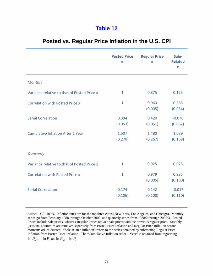
71

Table 12

Posted vs. Regular Price Inflation in the U.S. CPI

   

 Posted Price 

 

 Regular Price  

 

 Sale‐

Related 

   

 Monthly  

     

Variance relative to that of Posted Price   

1 0.875  0.125

Correlation with Posted Price   1 0.963             

(0.005) 

0.365     

(0.054) 

Serial Correlation  0.394          

(0.053) 

0.420           

(0.051) 

‐0.076     

(0.062) 

Cumulative Inflation After 1 Year   1.507       

(0.270) 

1.480            

(0.267) 

1.089

(0.168) 

 Quarterly  

     

Variance relative to that of Posted Price   

1 0.925  0.075

Correlation with Posted Price   1 0.979            

(0.005) 

0.285      

(0.100) 

Serial Correlation    

0.174          

(0.106) 

0.142             

(0.108) 

‐0.017     

(0.110) 

Source: CPI-RDB. Inflation rates are for the top three cities (New York, Los Angeles, and Chicago). Monthly series go from February 1988 through October 2009, and quarterly series from 1988:2 through 2009:3. Posted Prices include sale prices, whereas Regular Prices replace sale prices with the previous regular price. Monthly (seasonal) dummies are removed separately from Posted Price Inflation and Regular Price Inflation before moments are calculated. “Sale-related inflation” refers to the series obtained by subtracting Regular Price Inflation from Posted Price Inflation. The “Cumulative Inflation After 1 Year” is obtained from regressing

12ln lnt tP P on 1ln lnt tP P .

72

Table 13

Posted vs. Reference Price Inflation in the U.S. CPI

   

 Posted Price  

 

 Reference Price  

 

 Non‐

Reference 

   

 Monthly  

     

Variance relative to that of Posted Price  1 0.462  0.538

Correlation with Posted Price   1 0.689              

(0.033) 

0.734     

(0.029) 

Serial Correlation  0.398          

(0.054) 

0.461           

(0.050) 

0.119       

(0.063) 

Cumulative Inflation After 1 Year  1.569     

(0.281) 

3.067           

(0.395) 

0.906

(0.162) 

 Quarterly  

     

Variance relative to that of Posted Price  

1 0.592  0.408

Correlation with Posted Price   1 0.822            

(0.037) 

0.642      

(0.066) 

Serial Correlation  0.175         

(0.109) 

0.441             

(0.091) 

‐0.217     

(0.107) 

Source: CPI-RDB. Inflation rates are for the top three cities (New York, Los Angeles, and Chicago). Monthly series go from August 1988 through April 2009, and quarterly series from 1988:3 through 2009:1. Reference Prices represent the most common price in the 13 month window centered on the current month for each item. Monthly (seasonal) dummies are removed separately from Posted Price Inflation and Reference Price Inflation before moments are calculated. “Non-reference Inflation” refers to the series obtained by subtracting Reference Price Inflation from Posted Price Inflation. The “Cumulative Inflation After 1 Year” is obtained from regressing

12ln lnt tP P on 1ln lnt tP P .

73

Table 14

Model Features and the Facts

   

Consistent Features 

 

 

Inconsistent Features 

     

Half of prices change only a few times a year 

 

 

Menu costs; 

Sticky input prices 

Price indexation; 

Convex adjustment costs 

Temporary price changes are common 

 

 

Sticky set; 

Price discrimination 

Menu costs with 

 flexible marginal cost 

Frequency differs persistently across goods 

 

 

Menu costs; 

Sticky information 

Exogenous frequency  

of price changes 

Price changes are large on average 

 

 

Big menu costs; 

Rational inattention 

Small idiosyncratic shocks with  

strong complementarities 

Many price changes are small 

 

 

Sticky information; 

Sticky path 

Large menu costs for changing  

each individual price 

Relative price changes are transitory 

 

 

Transitory   

Idiosyncratic shocks  

Strong micro  

complementarities 

Price changes are not well synchronized 

 

 

Big idiosyncratic   

shocks  

Small idiosyncratic shocks with 

strong complementarities  

Old prices do not change by bigger amounts 

 

 

Menu costs; 

Lumpy shocks 

Time‐dependent pricing with 

persistent shocks 

     

74

Source: CPI-RDB. Data are for the top three cities (New York, Los Angeles, and Chicago) January 1988 through October 2009. Each bar corresponds to an ELI product category (weighted by expenditure), and price change frequency is calculated as the weighted average across quotes within the ELI. Prices include sales and regular prices.

75

Source: CPI-RDB. Data are for the top three cities (New York, Los Angeles, and Chicago) January 1988 through October 2009. Each circle is one of eight Major Groups in the CPI (1998-onward definition), with the area proportional to the average expenditure weight over the sample. Prices include sales and regular prices. Frequency is calculated as the weighted mean across ELIs (with each ELI mean itself a weighted average across quotes within the ELI). Durability is based on estimates reported in Bils and Klenow (1998).

76

Source: CPI-RDB. Data are for the top three cities (New York, Los Angeles, and Chicago) January 1988 through October 2009. Each circle is one of eight Major Groups in the CPI (1998-onward definition), with the area proportional to the average expenditure weight over the sample. Prices include sales and regular prices. Frequency is calculated as the weighted mean across ELIs (with each ELI mean itself a weighted average across quotes within the ELI). Cyclicality is based on an OLS regression coefficient for each Major Group of real monthly consumption growth on aggregate real monthly consumption growth, using seasonally adjusted Detailed Expenditure data from the U.S. National Income and Product Accounts, January 1990 through May 2009.

77

Notes: Each data point represents one study from Table 1, with the Gouvea (2007) study excluded because of its overlap with the Barros et al. (2009) study. The monthly frequency of price change is as reported in Table 1, while the monthly rate of inflation is based on authors’ calculations.

78

Source: CPI-RDB. Data are for the top three cities (New York, Los Angeles, and Chicago), based on regular prices for processed items. We first calculated the monthly frequency of price changes (weighted mean across ELIs) from April 1988 through September 2009. We then took out seasonal (monthly) dummies, and calculated deviations from them. Finally, we averaged the monthly deviations in each quarter, and added back the mean across all quarters, to produce quarterly data from 1988:2 through 2009:3.

79

Source: CPI-RDB. Data are for the top three cities (New York, Los Angeles, and Chicago) for the quarters 1988:3 through 2009:1. Posted price inflation includes sale and regular prices. Reference price inflation is based on replacing the current posted price with the modal price in the 13-month window centered on the current month (for each micro datapoint). Inflation rates were calculated at the monthly level, and monthly (seasonal) dummies were removed for each series separately. The monthly residuals were summed to create quarterly data.

80

References

Álvarez, Luis J. (2008), “What Do Micro Price Data Tell Us on the Validity of the New Keynesian Phillips Curve?” Economics – The Open-Access, Open-Assessment E-Journal 2(19).

Álvarez, Luis J. and Ignacio Hernando (2004), “Price Setting Behaviour in Spain: Stylized

Facts using Consumer Price Micro-data,” Banco de España Working Paper 0422. Álvarez, Luis J. and Ignacio Hernando (2006), “Price Setting Behaviour in Spain. Evidence

from Consumer Price Micro-data,” Economic Modelling 23: 699-716. Álvarez, Luis J. and Ignacio Hernando (2007a), “The Price Setting Behaviour of Spanish

Firms: Evidence from Survey Data,” Pricing Decisions in the Euro Area: How Firms Set Prices and Why, Oxford University Press, S. Fabiani, C. Loupias, F. Martins, and R. Sabbatini, eds.

Álvarez, Luis J. and Ignacio Hernando (2007b), “Competition and Price Adjustment in the

Euro Area,” Pricing Decisions in the Euro Area: How Firms Set Prices and Why, Oxford University Press, S. Fabiani, C. Loupias, F. Martins, and R. Sabbatini, eds.

Álvarez, L.J., P. Burriel and Ignacio Hernando (2008), “Price Setting Behaviour in Spain:

Evidence From Micro PPI Data,” forthcoming in Managerial and Decision Economics. Amirault, D., C. Kwan, and G. Wilkinson (2006), “Survey of Price-Setting Behaviour of

Canadian Companies,” Bank of Canada Working Paper 2006-35. Apel, Mikael, Richard Friberg, and Kerstin Hallsten (2005), “Microfoundations of

Macroeconomic Price Adjustment: Survey Evidence from Swedish Firms,” Journal of Money, Credit and Banking, 37 (April): 313-338.

Aucremanne, Luc and Emmanuel Dhyne (2004), “How Frequently Do Prices Change?

Evidence Based on the Micro Data Underlying the Belgian CPI,” ECB Working Paper 331. Aucremanne, Luc and Martine Druant (2005), “Price-Setting Behaviour in Belgium: What

Can be Learned from an Ad Hoc Survey,” ECB Working Paper 448. Baharad, Eyal and Benjamin Eden (2004), “Price Rigidity and Price Dispersion: Evidence

from Micro Data,” Review of Economic Dynamics 7 (July): 613-641. Ball, Laurence and N. Gregory Mankiw (1995), “Relative-Price Changes as Aggregate

Supply Shocks,” Quarterly Journal of Economics 110 (February): 161-193. Ball, Laurence and David Romer (1990), “Real Rigidities and the Non-neutrality of Money,”

Review of Economic Studies 57 (April): 183-203.

81

Barro, Robert J. (1977), “Long-term Contracting, Sticky Prices and Monetary Policy,” Journal of Monetary Economics 3 (July): 305-316.

Barros, Rebecca, Marco Bonomo, Carlos Carvalho, and Silvia Matos (2009), “Price Setting in

a Variable Macroeconomic Environment: Evidence from Brazilian CPI,” unpublished paper, Getulio Vargas Foundation and Federal Reserve Bank of New York.

Barsky, Robert, Christopher L. House, and Miles Kimball (2007), “Sticky-Price Models and

Durable Goods,” American Economic Review 97 (June): 984-998. Baudry, Laurent, Hervé Le Bihan, Patrick Sevestre and Sylvie Tarrieu (2007), “What Do

Thirteen Million Price Records Have to Say about Consumer Price Rigidity?” Oxford Bulletin of Economics and Statistics 69 (2): 139-183.

Baumgartner, Josef, Ernst Glatzer, Fabio Rumler, and Alfred Stiglbauer (2005), “How

Frequently Do Consumer Prices Change in Austria? Evidence from Micro CPI Data,” ECB Working Paper 523.

Bernanke, Ben S., Jean Boivin, and Piotr Eliasz (2005), “Measuring the Effects of Monetary

Policy: A Factor-Augmented Vector Autoregressive (FAVAR) Approach,” Quarterly Journal of Economics 120 (February): 387-422.

Bils, Mark (2004), “Studying Price Markups from Stockout Behavior,” unpublished paper,

University of Rochester (December). Bils, Mark and Peter J. Klenow (1998), “Using Consumer Theory to Test Competing

Business Cycle Models,” Journal of Political Economy 103 (April): 233-261. Bils, Mark and Peter J. Klenow (2004), “Some Evidence on the Importance of Sticky Prices,”

Journal of Political Economy 112 (October): 947-985. Bils, Mark, Peter J. Klenow, and Oleksiy Kryvtsov (2003), “Sticky Prices and Monetary

Policy Shocks,” Federal Reserve Bank of Minneapolis Quarterly Review (Winter): 2-9. Bils, Mark, Peter J. Klenow, and Benjamin A. Malin (2009), “Reset Price Inflation and the

Impact of Monetary Policy Shocks,” NBER Working Paper 14787. Blinder, Alan S., Elie Canetti, David Lebow, and Jeremy Rudd (1998), Asking About Prices:

A New Approach to Understanding Price Stickiness. New York: Russell Sage Foundation. Boivin, Jean, Robert Clark and Nicolas Vincent (2009), “Virtual Borders: Online Nominal

Rigidities and International Market Segmentation,” unpublished paper, HEC Montreal. Boivin, Jean, Marc Giannoni and Ilian Mihov (2009), “Sticky Prices and Monetary Policy:

Evidence from Disaggregated U.S. Data,” American Economic Review 99 (March): 350-384.

82

Broda, Christian and David Weinstein (2007), “Product Creation and Destruction: Evidence

and Price Implications,” NBER Working Paper 13041. Buckle, Robert A. and John A. Carlson (2000), “Menu Costs, Firm Size and Price Rigidities,”

Economics Letters, 66 (January): 59-63. Bunn, Philip and Colin Ellis (2009), “Price-Setting Behaviour in the United Kingdom: A

Microdata Approach,” Bank of England Quarterly Bulletin, 2009 Q1. Burstein, Ariel (2006), “Inflation and Output Dynamics with State Dependent Pricing

Decisions,” Journal of Monetary Economics 53 (7/October): 1235-1257. Burstein, Ariel and Christian Hellwig (2007), “Prices and Market Shares in a Menu Cost

Model,” unpublished paper, UCLA. Burstein, Ariel and Nir Jaimovich (2009), “Understanding Movements in Aggregate and

Product-Level Real-Exchange Rates,” unpublished paper, UCLA and Stanford University. Calvo, Guillermo A. (1983), “Staggered Prices in a Utility-Maximizing Framework,” Journal

of Monetary Economics 12 (September): 383-398. Campbell, Jeffrey R. and Benjamin Eden (2005), “Rigid Prices: Evidence from U.S. Scanner

Data,” unpublished paper, Federal Reserve Bank of Chicago and Vanderbilt University. Carlton, Dennis W. (1986), “The Rigidity of Prices,” American Economic Review 76

(September): 637-658. Carvalho, Carlos (2006), “Heterogeneity in Price Stickiness and the Real Effects of Monetary

Shocks,” Frontiers of Macroeconomics 2(1), Article 1. Castanon, Vicente, José Antonio Murillo, and Javier Salas (2008), “Formacion de precios en

la industria manufacturer de Mexico,” El Trimestre Economico, 75(1): 143-181. Cavallo, Alberto (2009), “Scraped Online Data and Sticky Prices: Frequency, Hazards and

Synchronization,” unpublished paper, Harvard University. Cecchetti, Stephen G. (1986), “The Frequency of Price Adjustment: a Study of Newsstand

Prices of Magazines,” Journal of Econometrics 31 (April): 255-274. Christiano, Lawrence J., Martin Eichenbaum, and Charles Evans (1999), “Monetary Policy

Shocks: What Have We Learned and to What End?,” Handbook of Macroeconomics, volume 1A, Elsevier: New York, John B. Taylor and Michael Woodford, eds.

83

Christiano, Lawrence J., Martin Eichenbaum, and Charles Evans (2005), “Nominal Rigidities and the Dynamic Effects of Shocks to Monetary Policy,” Journal of Political Economy 113 (February): 1-45.

Copaciu, Mihai, Florian Neagu and Horia Braun-Erdei (2007), “Survey Evidence on Price

Setting Patterns of Romanian Firms,” unpublished paper, National Bank of Romania. Cornille, David and Maarten Dossche (2008), “Some Evidence on the Adjustment of

Producer Prices,” Scandinavian Journal of Economics 110 (September): 489-518. Creamer, Kenneth (2008), “Price Setting Behaviour in South Africa – Stylised Facts using

Producer Price Microdata,” unpublished paper, University of the Witwatersrand. Creamer, Kenneth and Neil A. Rankin (2008), “Price Setting in South Africa 2001–2007 -

stylised facts using consumer price micro data,” Journal of Development Perspectives, 1(4): 93-118.

Dabusinskas, Aurelijus and Martti Randveer (2006), “Comparison of Pricing Behaviour of

Firms in the Euro Area and Estonia,” Bank of Estonia Working Paper 2006-08. Dhyne, Emmanuel, Luis J. Álvarez, Hervé Le Bihan, Giovanni Veronese, Daniel Dias,

Johannes Hoffmann, Nicole Jonker, Patrick Lünnemann, Fabio Rumler and Jouko Vilmunen (2005), “Price Setting in the Euro Area: Some Stylized Facts from Individual Consumer Price Data,” ECB Working Paper 524.

Dhyne, Emmanuel, Luis J. Alvarez, Hervé Le Bihan, Giovanni Veronese, Daniel Dias,

Johannes Hoffmann, Nicole Jonker, Patrick Lunnemann, Fabio Rumler and Jouko Vilmunen (2006), “Price Changes in the Euro Area and the United States: Some Facts from Individual Consumer Price Data,” Journal of Economic Perspectives 20 (Spring): 171-192.

Dias, Mónica, Daniel Dias and Pedro D. Neves (2004), “Stylised Features of Price Setting

Behaviour in Portugal: 1992-2001,” ECB Working Paper 332. Domberger, Simon and Denzil G. Fiebig (1993), “The Distribution of Price Changes in

Oligopoly,” The Journal of Industrial Economics 41 (September): 295-313. Dotsey, Michael, Robert King and Alexander Wolman (1999), “State-Dependent Pricing and

the General Equilibrium Dynamics of Money and Output,” Quarterly Journal of Economics 114 (May): 655-690.

Druant, Martine, Silvia Fabiani, Gabor Kezdi, Ana Lamo, Fernando Martins, and Roberto

Sabbatini (2009), “How are Firms’ Wages and Prices Linked: Survey Evidence in Europe,” ECB Working Paper 1084 (August).

Eden, Benjamin (2001), “Inflation and Price Adjustment: An Analysis of Microdata,” Review

of Economic Dynamics 4 (October): 607 - 636.

84

Eichenbaum, Martin, Nir Jaimovich, and Sergio Rebelo (2009), “Reference Prices and

Nominal Rigidities,” unpublished paper, Northwestern Univserity and Stanford University. Fabiani, Silvia, Martine Druant, Ignacio Hernando, Claudia Kwapil, Bettina Landau, Claire

Loupias, Fernando Martins, Thomas Y. Mathä, Roberto Sabbatini, Harald Stahl, and Ad C. J. Stokman (2005), “The Pricing Behavior of Firms in the Euro Area: New Survey Evidence,” ECB Working Paper 535.

Fabiani, Silvia, Angela Gatulli, and Roberto Sabbatini (2007), “The Pricing Behavior of

Italian Firms. New Survey Evidence on Price Stickiness,” Pricing Decisions in the Euro Area: How Firms Set Prices and Why, Oxford University Press, S. Fabiani, C. Loupias, F. Martins, and R. Sabbatini, eds.

Fabiani, Silvia, Angela Gattulli, Roberto Sabbatini and Giovanni Veronese (2006),

“Consumer Price Setting in Italy,” Giornale degli Economisti e Annali di Economia 65 (1): 31-74.

Fisher, Timothy C.G. and Jerzy D. Konieczny (2000), “Synchronization of Price Changes by

Multiproduct Firms: Evidence from Canadian Newspaper Prices,” Economics Letters, 68: 271-277.

Fitzgerald, Doireann and Stefanie Haller (2009), “Pricing-to-Market: Evidence From

Producer Prices,” unpublished paper. Gabriel, Peter and Adam Reiff (2008), “Price setting in Hungary – a Store-level Analysis,”

unpublished paper, Magyar Nemzeti Bank. Gagnon, Etienne (2009), “Price Setting during Low and High Inflation: Evidence from

Mexico,” Quarterly Journal of Economics 124 (August): 1221 – 1263. Gautier, Erwan (2008), “The Behaviour of Producer Prices: Some Evidence from the French

PPI Micro Data,” Empirical Economics, 35 (September): 301-332. Gertler, Mark and John Leahy (2008), “A Phillips Curve with an Ss Foundation,” Journal of

Political Economy 116 (June): 533-572. Goldberg, Pinelopi K. and Rebecca Hellerstein (2009), “How Rigid are Producer Prices,”

FRBNY Staff Report 407. Golosov, Mikhail and Robert E. Lucas, Jr. (2007), “Menu Costs and Phillips Curves,”

Journal of Political Economy 115 (April): 171–199. Gopinath, Gita, Pierre-Olivier Gourinchas, Chang-Tai Hsieh, and Nicholas Li (2009),

“Estimating the Border Effect: Some New Evidence,” unpublished paper, Harvard University, University of California at Berkeley and University of Chicago.

85

Gopinath, Gita and Oleg Itskhoki (forthcoming), “Frequency of Price-Adjustment and Pass-

through,” Quarterly Journal of Economics. Gopinath, Gita, Oleg Itskhoki, and Roberto Rigobon (forthcoming), “Currency Choice and

Exchange Rate Pass-through,” American Economic Review. Gopinath, Gita and Roberto Rigobon (2008), “Sticky Borders,” Quarterly Journal of

Economics 123 (May): 531-575. Gouvea, Solange (2007), “Price Rigidity in Brazil: Evidence from CPI Micro Data,” Central

Bank of Brazil Working Paper 143. Hall, Simon, Mark Walsh and Anthony Yates (2000), “Are UK Companies’ Prices Sticky?”

Oxford Economic Papers 52 (3): 425-446. Guimaraes, Bernardo and Kevin D. Sheedy (2008), “Sales and Monetary Policy,” CEPR

Discussion Paper 6940. Hansen, Bo William and Niels Lynggard Hansen (2006), “Price Setting Behavior in

Denmark: A Study of CPI Micro Data 1997-2005,” Danmarks Nationalbank Working Paper 39.

Hobijn, Bart, Federico Ravenna, and Andrea Tambalotti (2006), “Menu Costs at Work:

Restaurant Prices and the Introduction of the Euro,” Quarterly Journal of Economics 121 (August): 1103 – 1131.

Hoeberichts, Marco and Ad Stokman (2006), “Pricing Behaviour of Dutch Companies:

Results of a Survey,” ECP Working Paper 607. Hoffmann, Johannes and Jeong-Ryeol Kurz-Kim (2006), “Consumer Price Adjustment under

the Microscope: Germany in a Period of Low Inflation,” ECB Working Paper 652. Horvath, Roman and Fabrizio Coricelli (2006), “Price Setting Behaviour: Micro Evidence on

Slovakia,” CEPR Discussion Papers 5445. Ikeda, Daisuke, and Shinichi Nishioka (2007), “Price Setting Behavior and Hazard Functions:

Evidence from Japanese CPI Micro Data,” Bank of Japan Working Paper 07-E-19. Jonker, Nicole, Carsten Folkertsma, and Harry Blijenberg (2004), “Empirical Analysis of

Price Setting Behaviour in the Netherlands in the Period 1998-2003 using Micro Data,” ECB Working Paper 413.

Julio, Juan Manuel and Hector Manuel Zárate (2008), “The Price Setting Behaviour in

Colombia: Evidence from PPI Micro Data,” Borradores de Economía. Banco de la República. Colombia.

86

Kashyap, Anil K. (1995), “Sticky Prices: New Evidence from Retail Catalogues,” Quarterly

Journal of Economics 110 (February): 245-274. Kehoe, Patrick J. and Virgiliu Midrigan (2008), “Temporary Price Changes and the Real

Effects of Monetary Policy,” Federal Reserve Bank of Minneapolis Research Department Staff Report 413 (September).

Kimball, Miles S. (1995), “The Quantitative Analytics of the Basic Neomonetarist Model,”

Journal of Money, Credit, and Banking 27 (November): 1241-1277. Klenow, Peter J. and Kryvtsov, Oleksiy (2008), “State-Dependent or Time-Dependent

Pricing: Does It Matter For Recent U.S. Inflation?” Quarterly Journal of Economics 123 (August): 863-904.

Klenow, Peter J. and Jonathan L. Willis (2006), “Real Rigidities and Nominal Price

Changes,” unpublished paper, Stanford University and Federal Reserve Bank of Kansas City.

Klenow, Peter J. and Jonathan L. Willis (2007), “Sticky Information and Sticky Prices,”

Journal of Monetary Economics 54 (September): 79-99. Konieczny, Jerzy D. and Andrzej Skrzypacz (2005), “Inflation and Price Setting in a Natural

Experiment,” Journal of Monetary Economics 52 (April): 621-632. Kovanen, Arto (2006), “Why Do Prices in Sierra Leone Change so Often? A Case Study

using Micro-level Price Data,” International Monetary Fund Working Paper 06/53. Kryvtsov, Oleksiy and Virgiliu Midrigan (2009), “Inventories, Markups, and Real Rigidities

in Menu Cost Models,” unpublished paper, Bank of Canada. Kwapil, Claudia, Josef Baumgartner and Johann Scharler (2005), “The Price-setting

Behaviour of Austrian Firms: Some Survey Evidence,” ECB Working Paper 464. Lach, Saul and Daniel Tsiddon (1992), “The Behavior of Prices and Inflation: An Empirical

Analysis of Disaggregated Price Data,” Journal of Political Economy 100 (April): 349 – 389.

Lach, Saul and Daniel Tsiddon (1996), “Staggering and Synchronization in Price-Setting:

Evidence from Multiproduct Firms,” American Economic Review 86 (December): 1175 – 1196.

Levy, Daniel, Shantanu Dutta, Mark Bergen, and Robert Venable (1998), “Price Adjustment

and Multiproduct Retailers,” Managerial and Decision Economics 19: 81-120.

87

Levy, Daniel, Dongwon Lee, Haipeng (Allan) Chen, Robert J. Kauffman, and Mark Bergen (2007), “Price Points and Price Rigidity,” Working Paper 04-07, The Rimini Center for Economic Analysis.

Loupias, Claire and Roland Ricart (2004), “Price Setting in France: New Evidence from

Survey Data,” ECB Working Paper 423. Lünnemann, Patrick and Thomas Y. Mathä (2005), “Consumer Price Behaviour in

Luxembourg: Evidence from Micro CPI Data,” ECB Working Paper 541. Lünnemann, Patrick and Thomas Y. Mathä (2006), “New Survey Evidence on the Pricing

Behavior of Luxenbourg Firms,” ECB Working Paper 617. Lünnemann, Patrick and Ladislav Wintr (2006), “Are Internet Prices Sticky?” ECB Working

Paper 645. Mackowiak, Bartosz and Frank Smets (2008), “Implications of Micro Price Data for

Macroeconomic Models,” CEPR Discussion Paper 6961. Mackowiak, Bartosz and Mirko Wiederholt (2008), “Business Cycle Dynamics Under

Rational Inattention,” unpublished paper, European Central Bank and Northwestern University.

Mankiw, N. Gregory, and Ricardo Reis (2002), “Sticky Information versus Sticky Prices: A

Proposal to Replace the New Keynesian Phillips Curve,” Quarterly Journal of Economics 117 (November), 1295-1328.

Martins, Fernando (2005), “The Price Setting Behavior of Portuguese Firms: Evidence from

Survey Data,” ECP Working Paper 562. Medina, Juan Pablo, David Rappoport, and Claudio Soto (2007), “Dynamics of Price

Adjustment: Evidence from Micro Level Data for Chile,” Central Bank of Chile Working Paper 432.

Midrigan, Virgiliu (2009), “Menu Costs, Multiproduct Firms, and Aggregate Fluctuations,”

unpublished paper, New York University. Nakagawa, Shinobu, Ryota Hattori, and Izumi Takagawa (2000), “Price Setting Behavior of

Japanese Companies,” research paper, Bank of Japan. Nakamura, Emi (2008), “Pass-Through in Retail and Wholesale,” American Economic

Review 98 (May): 430-437. Nakamura, Emi and Jón Steinsson (2008a), “Five Facts About Prices: A Reevaluation of

Menu Cost Models,” Quarterly Journal of Economics 123 (November): 1415-1464.

88

Nakamura, Emi and Jón Steinsson (2008b), “Monetary Non-Neutrality in a Multi-Sector Menu Cost Model,” NBER Working Paper 14001 (May).

Nakamura, Emi and Jón Steinsson (2009), “Lost in Transit: Product Replacement Bias and

Pricing to Market,” unpublished paper, Columbia University. Nakamura, Emi and Dawit Zerom (forthcoming), “Accounting for Incomplete Pass-Through,”

Review of Economic Studies. Peersman, Gert and Frank Smets (2003), “The Monetary Transmission Mechanism in the

Euro Area: More Evidence from VAR Analysis,” Monetary Policy Transmission in the Euro Area, Cambridge University Press: Cambridge, I. Angeloni, A. Kashyap, and B. Mojon, eds.

Peneva, Ekaterina (2009), “Factor Intensity and Price Rigidity: Evidence and Theory,” FEDS

Working Paper No. 2009-07 (January). Romer, David H. and Christina D. Romer (2004), “A New Measure of Monetary Shocks:

Derivation and Implications,” American Economic Review 94 (September): 1055-1084. Rotemberg, Julio J. (1982), “Monopolistic Price Adjustment and Aggregate Output,” Review

of Economic Studies, 49 (October): 517-531. Sabbatini, Roberto, Silvia Fabiani, Angela Gatulli, and Giovanni Veronese (2006), “Producer

Price Behaviour in Italy: Evidence From Micro PPI Data,” unpublished paper, Banca d’Italia.

Sahinoz, Saygin and Bedriye Saracoglu (2008), “Price Setting Behaviour in Turkish

Industries: Evidence from Survey Data,” Turkish Economic Association Discussion Paper 2008/3.

Saita, Yumi, Izumi Takagawa, Kenji Nishizaki, and Masahiro Higo (2006), “Price Setting in

Japan: Evidence from Individual Retail Price Data,” Bank of Japan Working Paper Series, No. 06-J-02, (in Japanese).

Stahl, Harald (2005), “Price Setting in German Manufacturing: New Evidence from New

Survey Data”, Discussion Paper 43/2005, Deutsche Bundesbank. Stahl, Harald (2006), “Producer Price Adjustment at the Micro Level: Evidence from

Individual Price Records Underlying the German PPI”, unpublished paper, Deutsche Bundesbank.

Taylor, John B. (1980), “Aggregated Dynamics and Staggered Contracts,” Journal of

Political Economy 88 (February): 1-24.

89

Vermeulen, Philip, Daniel Dias, Maarten Dossche, Erwan Gautier, Ignacio Hernando, Roberto Sabbatini and Harald Stahl (2007), “Price Setting in the Euro Area: Some Stylized Facts from Individual Producer Price Data,” ECB Working Paper 727.

Vilmunen, Jouko and Helinä Laakkonen (2005), “How Often Do Prices Change in Finland?

Micro-level Evidence from the CPI,” unpublished paper, Bank of Finland. Woodford, Michael (2009), “Information-Constrained State-Dependent Pricing,” Journal of

Monetary Economics 56 (October): S100-S124. Wolman, Alexander (2007), “The Frequency and Costs of Individual Price Adjustment,”

Managerial and Decision Economics 28 (6): 531-552. Wulfsberg, Fredrik (2009), “Price Adjustments and Inflation: Evidence from Consumer Price

Data in Norway 1975-2004,” Norges Bank WP 2009/11.