Microdynamics and Thermal Snap Response of...

Microdynamics and Thermal Snap Response ofDeployable Space Structures

by

Michel D. Ingham

B. Eng. Mechanical Engineering (Honours)McGill University, 1995

Submitted to the Department of Aeronautics and Astronauticsin partial fulfillment of the requirements for the degree of

MASTER OF SCIENCE IN AERONAUTICS AND ASTRONAUTICSAT THE

MASSACHUSETTS INSTITUTE OF TECHNOLOGY

May 1998

© 1998 Massachusetts Institute of TechnologyAll rights reserved

Signature of Author …………………………………………………………………………………Department of Aeronautics and Astronautics

May 15, 1998

Certified by …………………………………………………………………………………………Professor Edward F. Crawley

Department of Aeronautics and AstronauticsThesis Supervisor

Accepted by ………………………………………………………………………………………...Professor Jaime Peraire

Chairman, Department Graduate Committee

3

Microdynamics and Thermal Snap Response

of Deployable Space Structures

by

Michel D. Ingham

Submitted to the Department of Aeronautics and Astronauticson May 15, 1998 in Partial Fulfillment of the Requirements for

the Degree of Master of Science in Aeronautics and Astronautics

Abstract

Due to the size constraints imposed by the payload bays of carrier spacecraft, future precisionspace structures (e.g. interferometric telescopes) will undoubtedly require some form of on-orbitdeployment mechanism, including joints or hinges which will introduce nonlinearity to thestructure. Results are presented from a two-part experimental investigation of the microdynamicresponse of nonlinear structures, to both mechanical and thermal excitation sources.

In the first experiment, the dynamic response of a deployable truss at sub-microstrain levels ofvibration is characterized in terms of modal parameters. The test article is subjected to stepped-sine sweeps through its fundamental flexible modes over a range of excitation amplitudes. High-sensitivity piezoceramic strain sensors are used in conjunction with a lock-in amplifier to measurethe truss response from tens of microstrain down to one nanostrain. The natural frequency anddamping ratio are computed from the frequency response functions, using a circle fit method.Results show that the values of the modal parameters are strain-dependent at high responseamplitudes, and strain-independent at low amplitudes. It is inferred that, at microdynamic levelsof excitation, the internal loads needed to overcome the joint friction are not attained. Thenonlinear mechanisms in the structure are thus not activated, resulting in a linear truss response.

In the second experiment, the phenomenon of thermal snap, or creak, is investigated. Thermalsnap is a disturbance which occurs when thermally-induced stress in a statically indeterminatestructure is suddenly released via a slip internal to a joint or other frictional mechanism. Arepresentative deployable truss is suspended in a thermal chamber, where its temperature iscycled between –30°C and 50°C, in order to determine whether thermal snap occurs in such astructure. High-bandwidth accelerometers distributed across the truss are used as the primarysensors for detecting structural events. Thermal snaps are found to occur during the thermaltransients, before steady-state is achieved throughout the truss. The truss response to theimpulsive and broadband disturbances is characterized in both the time and frequency domains.The transient response exhibits telltale signs of structural behavior, including multi-mode ordominant-mode excitation, and reasonable modal damping in the time decay.

Thesis Supervisor: Edward F. CrawleyTitle: Professor of Aeronautics and Astronautics

5

Acknowledgements

I would like to express utmost appreciation to my advisor, Professor Edward Crawley, for his

guidance and support, in matters academic and otherwise. I also owe a debt of gratitude to

Professor David Miller, Director of the MIT Space Systems Lab, for his invaluable advice and

faith in my abilities. A special thank-you goes to Yool Kim, with whom I worked on the thermal

snap experiment, for the hours of enlightening discussion which filled the (sometimes lengthy)

gaps between snap events. A hearty round of thanks is due to Marthinus van Schoor, Javier de

Luis and the folks at Payload Systems Inc. and Midé Technology Corp., as well as Ed Mencow,

Ron Efromson, Jon Howell and Al Mason from MIT Lincoln Laboratory, for their patience and

generosity in allowing us to use their facilities for the thermal snap experiment. Their assistance

was greatly appreciated.

This research was sponsored under Jet Propulsion Laboratory grant #960747, with Dr. Marie

Levine-West as technical monitor. I would like to extend a personal note of appreciation to Marie

for her helpful input and interest in my work. The National Sciences and Engineering Research

Council of Canada and the Canadian Space Agency are acknowledged, for contributing to the

support of my research in the form of an NSERC postgraduate scholarship and supplement.

I am also grateful for the help I received from members of the technical staff of the Department of

Aeronautics and Astronautics. In particular, many thanks to Paul Bauer, for passing along some

of his experimental know-how. I would certainly be remiss in forgetting to thank SharonLeah

Brown for going above and beyond the call of duty in her efforts to make life happy for the

graduate students in the Space Systems Lab and Active Materials and Structures Lab. To my

labmates, I would like to say how fortunate I am to have worked or otherwise interacted with all

of you.

And last but certainly not least, I would like to thank my family and friends for being an endless

source of encouragement.

7

Table of Contents

Acknowledgements..................................................................................................................... 5

Table of Contents........................................................................................................................ 7

List of Tables.............................................................................................................................. 9

List of Figures .......................................................................................................................... 11

Chapter 1 – Introduction ........................................................................................................... 15

1.1 Importance of Microdynamics......................................................................................... 15

1.2 Background..................................................................................................................... 17

1.3 Approach......................................................................................................................... 21

Chapter 2 – Modal Parameter Characterization.......................................................................... 23

2.1 Hardware Description and Experimental Setup ................................................................ 24

2.1.1 MODE Truss Testbed................................................................................................ 24

2.1.2 Actuators .................................................................................................................. 33

2.1.3 Sensors ..................................................................................................................... 35

2.1.4 Other Instrumentation................................................................................................ 38

2.2 Test Procedure................................................................................................................. 39

2.3 Precision and Accuracy of Measurements ........................................................................ 46

2.4 Experimental Results .......................................................................................................55

2.4.1 Discussion of Results ................................................................................................ 55

2.4.2 Correlation with Previous Results.............................................................................. 77

Chapter 3 – Thermal Snap Characterization .............................................................................. 83

3.1 Hardware Description and Experimental Setup ................................................................ 84

3.1.1 Structural hardware ................................................................................................... 84

3.1.2 Thermal Source......................................................................................................... 88

3.1.3 Sensors and data acquisition...................................................................................... 91

3.2 Test Procedure................................................................................................................. 94

3.3 Measures Taken to Identify Thermal Snap ..................................................................... 105

3.4 Experimental Results ..................................................................................................... 110

3.4.1 Tap Test Results...................................................................................................... 110

8

3.4.2 Convection Test Results .......................................................................................... 114

3.4.3 Radiation Test Results............................................................................................. 124

3.4.4 Summary of Findings .............................................................................................. 132

Chapter 4 – Conclusions ......................................................................................................... 135

4.1 Microdynamic Results ................................................................................................... 135

4.2 Implications for Future Precision Space Structures......................................................... 136

4.3 Recommendations for Future Work ............................................................................... 140

References.............................................................................................................................. 141

Appendix A – Modal Parameter Characterization Results....................................................... 145

Appendix B – Thermal Snap Characterization Results............................................................ 163

9

List of Tables

Table 2.1 Torsion mode results .................................................................................................63

Table 2.2 Bending mode results ................................................................................................ 73

Table 2.3 Repeatability test results............................................................................................ 77

Table 2.4 Comparison of results for MODE STA truss.............................................................. 78

Table 2.5 Comparison of accelerometer and piezo strain gauge data.......................................... 79

11

List of Figures

Figure 1.1 Simplified structural model illustrating thermal snap ................................................ 17

Figure 2.1 MODE STA baseline configuration.......................................................................... 24

Figure 2.2 First torsion and bending modes for the MODE STA................................................ 25

Figure 2.3 Partially collapsed deployable module...................................................................... 26

Figure 2.4 Deployable longeron................................................................................................ 26

Figure 2.5 Knee joint and latch mechanism............................................................................... 27

Figure 2.6 Batten frame corner fittings (intermediate and end bay) ............................................ 27

Figure 2.7 Cable termination detail ........................................................................................... 28

Figure 2.8 Tensioning lever detail .............................................................................................28

Figure 2.9 Force-state data for deployable bay [31] ................................................................... 29

Figure 2.10 Erectable strut ........................................................................................................ 30

Figure 2.11 Force-state data for erectable bay with loosened joints [31] .................................... 30

Figure 2.12 Suspended truss...................................................................................................... 31

Figure 2.13 Rigid appendage..................................................................................................... 32

Figure 2.14 Electro-magnetic shaker ......................................................................................... 33

Figure 2.15 Butterfly shaker...................................................................................................... 34

Figure 2.16 Dynamics of Butterfly shaker ................................................................................. 35

Figure 2.17 Instrumented strut .................................................................................................. 36

Figure 2.18 Sensor locations ..................................................................................................... 37

Figure 2.19 Flow of commands and information through the experiment setup.......................... 40

Figure 2.20 Torsion mode TF data with SDOF resonance fit ..................................................... 44

Figure 2.21 Polar plot of torsion mode TF data with circle fit .................................................... 44

Figure 2.22 Scatter plot of damping estimates from circle fit ..................................................... 45

Figure 2.23 Transmissibility TF from ceiling to truss ................................................................ 49

Figure 2.24 Elastic cord to offset weight of umbilical connector................................................ 51

Figure 2.25 Circle fit to noisy data ............................................................................................ 53

Figure 2.26 Typical transfer function data (torsion mode, high amplitude)................................. 57

Figure 2.27 Typical piezo output data (torsion mode, high amplitude) ....................................... 57

12

Figure 2.28 Typical load cell output data (torsion mode, high amplitude) .................................. 57

Figure 2.29 Typical transfer function sweep data (torsion mode, high amplitude) ...................... 58

Figure 2.30 Typical circle fit to transfer function (torsion mode, high amplitude) ...................... 58

Figure 2.31 Typical scatter of damping from circle fit to transfer function

(torsion mode, high amplitude) ............................................................................... 58

Figure 2.32 Typical piezo output sweep data (torsion mode, high amplitude)............................. 59

Figure 2.33 Typical circle fit to piezo output (torsion mode, high amplitude)............................. 59

Figure 2.34 Typical scatter of damping from circle fit to piezo output

(torsion mode, high amplitude) ............................................................................... 60

Figure 2.35 Typical transfer function data (torsion mode, low amplitude).................................. 61

Figure 2.36 Typical piezo output data (torsion mode, low amplitude) ........................................ 61

Figure 2.37 Typical load cell output data (torsion mode, low amplitude) ................................... 61

Figure 2.38 Typical piezo output sweep data (torsion mode, low amplitude).............................. 62

Figure 2.39 Typical circle fit to piezo output (torsion mode, low amplitude).............................. 62


(torsion mode, low amplitude) ................................................................................ 62

Figure 2.41 Modal parameters from TF data vs. strain amplitude (torsion mode) ....................... 64

Figure 2.42 Modal parameters from piezo output data vs. strain amplitude (torsion mode)......... 64

Figure 2.43 Typical piezo output data (bending mode, high amplitude, E-M shaker) ................. 67

Figure 2.44 Typical piezo output sweep data (bending mode, high ampl, E-M shaker)............... 68

Figure 2.45 Typical circle fit to piezo output (bending mode, high ampl, E-M shaker)............... 68


(bending mode, high ampl, E-M shaker) ................................................................. 68

Figure 2.47 Typical piezo output data (bending mode, high amplitude, B-fly shaker) ................ 69

Figure 2.48 Typical piezo output sweep data (bending mode, high ampl, B-fly shaker).............. 70

Figure 2.49 Typical circle fit to piezo output (bending mode, high ampl, B-fly shaker).............. 70


(bending mode, high ampl, B-fly shaker) ................................................................ 70

Figure 2.51 Typical piezo output data (bending mode, low amplitude, B-fly shaker) ................. 71

Figure 2.52 Typical piezo output sweep data (bending mode, low ampl, B-fly shaker)............... 72

Figure 2.53 Typical circle fit to piezo output (bending mode, low ampl, B-fly shaker)............... 72


(bending mode, low ampl, B-fly shaker) ................................................................. 72

Figure 2.55 Modal parameters from piezo output data vs. strain amplitude (bending mode)....... 74

13

Figure 2.56 SERC Interferometer Testbed (top view) ................................................................ 81

Figure 2.57 Microdynamic test results (erectable truss, high ampl) [21]..................................... 82

Figure 2.58 Microdynamic test results (erectable truss, low ampl) [21]...................................... 82

Figure 3.1 Dummy erectable truss bay ...................................................................................... 86

Figure 3.2 Detail of spring connection....................................................................................... 87

Figure 3.3 Noise due to convection chamber ............................................................................. 89

Figure 3.4 Deployable truss suspended in thermal vacuum chamber .......................................... 90

Figure 3.5 Typical convection thermal cycles............................................................................ 97

Figure 3.6 Typical uncontrolled radiation thermal cycle ............................................................ 99

Figure 3.7 Time trace and spectrogram of sample snap event .................................................. 101

Figure 3.8 Truncated sample data (256-point windows)........................................................... 102

Figure 3.9 Truncated and filtered transient event data.............................................................. 104

Figure 3.10 Exponentially-decaying sinusoid fit to filtered event............................................. 105

Figure 3.11 Sample electrical event......................................................................................... 109

Figure 3.12 Sensor and tap locations for tap tests .................................................................... 112

Figure 3.13 Response to Tap #1 .............................................................................................. 113

Figure 3.14 Response to Tap #2 .............................................................................................. 113

Figure 3.15 Temperature profile for typical convection test (June 23, 1997)............................ 115

Figure 3.16 Sensor distribution for typical convection test (June 23, 1997).............................. 115

Figure 3.17 Thermal snap data from typical convection test (June 23, 1997)............................ 116

Figure 3.18 Temperature profile for typical convection test (September 2, 1997)..................... 118

Figure 3.19 Sensor distribution for typical convection test (September 2, 1997)...................... 119

Figure 3.20a Thermal snap data from typical convection test (September 2, 1997).................. 120

Figure 3.20b Thermal snap data from typical convection test (September 2, 1997).................. 121

Figure 3.21 Temperature profiles from typical radiation test (September 29,1997).................. 125

Figure 3.22 Sensor distribution for typical radiation test (September 29, 1997)........................ 125

Figure 3.23 Thermal snap data from typical radiation test (September 29, 1997)..................... 126

Figure 3.24 Temperature profiles from typical radiation test (November 25, 1997).................. 129

Figure 3.25 Sensor distribution for typical radiation test (November 25, 1997)........................ 129

Figure 3.26a Thermal snap data from typical radiation test (November 25, 1997).................... 130

Figure 3.26b Thermal snap data from typical radiation test (November 25, 1997).................... 131

Figure 4.1 “SIM Classic” concept [47] .................................................................................... 137

Figure 4.2 “Son of SIM” concept [48]..................................................................................... 137

15

Chapter 1 – Introduction

1.1 Importance of Microdynamics

The hunt for Earth-like planets orbiting other stars has come to the forefront of the space

community’s interest. This is one of the primary objectives of NASA’s Origins Program, which

will launch a number of space-based observatories, starting in the next decade. These missions

will employ both connected interferometers and large aperture telescopes with adaptive mirrors.

Due to the size constraints imposed by the payload bays of carrier spacecraft, these telescopes

will undoubtedly require some form of on-orbit deployment mechanism, including joints or

hinges which will introduce nonlinearity to the structure.

The success of the Origins missions will hinge on whether positioning of the optical elements can

be maintained to within fractions of the viewing wavelength. Consequently, any minute

disturbance will pose a serious threat to the stability of the precision optical systems. The

response of structures with nonlinear elements to such small disturbances has yet to be researched

in depth. In order to predict the structural response in this regime, and ultimately control the

structure, accurate models of the disturbances and the low-amplitude dynamics of the structure

must be developed. Such models can only result from thorough experimental characterizations of

the disturbance sources and the structure itself.

The term “microdynamics” has been coined to describe the dynamics of materials and structures

at levels of vibration smaller than those targeted by standard testing levels. A more quantitative

definition of microdynamics is given by Wang and Hadaegh [1]: the regime in which the

structural vibration amplitudes are in the micron or submicron range. It is often convenient to use

a nondimensional metric such as strain to quantify and compare the vibration levels from

different tests. Typical levels of strain achieved during standard dynamic tests are in the range

between 10 and 1000 microstrain. Microdynamic levels of interest therefore cover the strains on

the order of microstrain, or smaller. Depending on the size and requirements of the structural

system, information on the dynamics down to nanostrain levels, or lower, may be sought.

16

One of the many microdynamic-level disturbances of interest is the phenomenon commonly

referred to as thermal snap, or creak. Statically indeterminate structures with nonlinear friction

interfaces are vulnerable to this disturbance source. As the thermal load on such a structure

changes, perhaps due to the change in radiation environment as the spacecraft passes in or out of

the Earth’s shadow, the structure tries to contract or expand as dictated by the coefficients of

thermal expansion (CTE) of its components (see simplified model in Figure 1.1). Due to a

mismatch in CTE between components made of different materials, free thermal expansion is not

allowed to occur, and stresses are created in the structure. This stress buildup can also occur due

to non-uniform heating or cooling across a structure, even one composed of a single material,

perhaps as a result of partial shadowing. If there are frictional interfaces in the load path between

stressed elements, a level of internal load can be attained such that the static friction force is

exceeded. The two elements then experience a sudden slip along the friction interface, which

releases the built-up stress, until the slip is halted due to one of two reasons: either enough stress

is relieved such that the internal load falls below the level of the dynamic friction, or the end of

the frictional deadband is reached (i.e. the fixed boundary of the interface is contacted). This slip

releases some of the thermally-induced elastic energy stored in the stressed elements, and

translates an impulsive disturbance internal to the structure.

Thermal snap is a potentially serious problem in space structures, especially in deployable and

flexible structures. The poor understanding of this type of disturbance is exacerbated because

thermal creaks have rarely, if at all, been directly observed. Their nature must generally be

inferred from the spacecraft sensors, and the control system response [2]. Nonlinear joints with

deadbands, tensioning cables and pulleys, and other structural elements that depend on friction

and allow relative motion are all examples of potential creak elements that are common in space

structures. The ability to predict creak events and the resulting structural response, either

deterministically or in a statistical sense, would benefit the design of dimensionally stable space

structures.

The overall objective of this research, therefore, is to perform a microdynamic-level investigation

of structures with nonlinear mechanisms, representative of future precision space structures.

Specifically, the main goal is to experimentally characterize the dynamic response of a

deployable truss at sub-microstrain levels of vibration, due to mechanically- and thermally-

induced structural excitation.

17

T∆α EA

α EA2 2

1 1

Slip Slip

δx

x s x d

(A)

(B)

1

T∆2

(C) (D)

Figure 1.1 Simplified structural model illustrating thermal snap.

A potentially non-uniform temperature gradient is applied to a statically indeterminatestructure with CTE-mismatched components (A). Constrained thermal deformation δxoccurs, as internal stresses build up (B). Once a critical level of stress is reached, thefrictional interface slips. The slip halts after a relative displacement xs, if the internal loadfalls below the dynamic friction level (C), or xd, if the end of the joint deadband is reached(D).

1.2 Background

In the middle of the last decade, the field of microdynamics was born from the need for high-

precision structures in space: the standard structural testing methodologies of the time were

incapable of evaluating whether the new breed of spacecraft would satisfy their stringent stability

18

requirements. Since then, researchers have devoted considerable resources to develop facilities

and procedures which would allow them to design such spacecraft. In this section, past and

ongoing research in the fields of microdynamics and general structural dynamics is discussed, as

background for the study documented in this thesis.

The dynamics of structures with nonlinear mechanisms is a field which has matured considerably

since the early 1980s. Considerable work has focused on the characterization of such structures at

the mechanism- or component-level, as well as at the global structure-level. At the mechanism-

level, several types of joints that display nonlinear behavior have been analyzed. Hertz and

Crawley developed models of sleeve-stiffened and pinned joints, to investigate displacement-

dependent friction damping and impact losses [3]. Further analytical work on nonlinear sleeve

joints incorporated into flexible space structures was pursued by Ferri [4]. Tzou et al. modeled a

3-D spherical ball/socket joint, including friction and clearance effects [5]. The key problem with

joint models such as these is the difficulty in accurately characterizing the friction mechanisms

and other nonlinear joint behavior. Design-specific parameters such as the coefficient of friction

and joint deadband are difficult to predict. In general, they must be determined experimentally,

using methods such as force-state mapping [6, 7, 8]. An ongoing program at NASA Langley

Research Center focuses on developing key structure and mechanism technologies for micron-

accuracy, in-space deployment of future science intruments [9, 10]; one of the most recent results

of their efforts is a new design for precision revolute joints, which exhibit high linearity and

repeatability.

In addition to research on particular nonlinear mechanisms, a number of researchers have

developed techniques for modeling the global dynamics of joint-dominated truss structures, both

at “standard” and microdynamic levels. Wang and Hadaegh proposed a methodology for the

mathematical modeling of preloaded truss-based space structures, in the microdynamic regime

[1]. Their models incorporated monoball and butt joints, where the dynamic behavior was derived

from Hertzian contact theory. Chapman et al. employed a residual force technique to perform

transient analyses of trusses having joints with arbitrary force-state map characteristics [11]. The

time response of trusses with nonlinear joints was also analyzed by Belvin, using a nonlinear

finite element approach [12]. Sarver developed an analytic model for jointed space structures

based on continuous damped beams and a piecewise linear joint [13]; his model correlated well

with experimental results, which demonstrated dissipation and energy transfer between modes in

a structure due to the presence of joints. Structural nonlinearities have also been modeled using

19

the describing function technique, in which a quasi-linearization of the force-state characteristics

of the nonlinearity is performed [14, 15, 16].

Considerable experimental work has focused on the dynamics of jointed truss structures. Notably,

MIT’s Middeck 0-Gravity Dynamics Experiment (MODE) addressed the structural response of a

deployable truss test article at relatively large strain levels [17]. Linear and nonlinear models

were constructed, for both gravity and zero-gravity environments. Model accuracy was verified

by comparing the modeling results with the ground and on-orbit data obtained. In particular, the

effects of nonlinearities (due to the joint friction and slackening tension cables) on modal

parameters (frequency, damping) were investigated. These millimeter-to-micron-level dynamics

experiments also demonstrated that increased preload results in stiffening and decreased modal

damping. Component-level characterization of the structural nonlinearities was performed by

Masters, via the force-state mapping technique [18]. The results from the component

characterization experiments were used to generate dynamic models of the global truss behavior

[19].

Another space flight experiment, the Joint Damping Experiment (JDX), was developed by

researchers at Utah State University to measure the influence of gravity on the structural damping

of a truss with pinned joints [20]. The results from the ground and flight data indicated that

friction and impacting in the joints were primary sources of damping. In the absence of gravity

preload, increased damping was observed; greater freedom for impacting within the joint

deadbands was identified as the likely source of this increase in damping, as energy is transferred

to the higher-frequency modes excited by the impacting.

Damping within an erectable truss structure, subject to nanostrain levels of disturbance, was

characterized by Ting and Crawley [21]. This work, done on a tetrahedral interferometer testbed,

showed that structural damping is independent of strain below 1 microstrain, and increases with

strain above that level. One of the objectives of the study documented in this thesis is to verify

this conclusion for deployable trusses, where behavior may be significantly altered by the

frictional joint mechanisms required for deployment.

Warren and Peterson [22] performed an experimental characterization of the microdynamics of a

prototype deployable telescope support structure. They discovered that intentional application of

impulses to the structure induced abrupt changes in structural shape at the microdynamic level

20

(dubbed “micro-lurches”). Furthermore, their study illustrated that successive impulses applied to

the structure eventually brought the structure to a microdynamically stable position (the

“equilibrium zone”). They developed a model for this behavior, which suggests that these effects

were due to the dynamically-induced relaxation of strain energy stored by friction mechanisms

within the structure.

In his text titled “Thermal Structures for Aerospace Applications” [2], Thornton provides a

historical review of published work on the subject of thermally-induced structural disturbances.

Most of the documented research focused on the excitation of low-frequency modes of long and

slender structures, due to the application of sudden thermal gradients. This phenomenon has been

observed during orbital day-night or night-day transitions on numerous spacecraft, including the

OGOs spacecraft in the 1960s, and more recently, the Hubble Space Telescope [23]. This coupled

thermal-structural response has been replicated in laboratory environments by a few different

researchers, and has been alternately dubbed “thermal elastic shock” [24], or “thermal jitter” [25].

Another type of thermally-induced structural disturbance is thermal snap, or creak, which was

described in section 1.1. Very little work on this phenomenon has been documented, despite on-

orbit evidence of its occurrence: Foster et al. speculated that the Hubble Space Telescope

experienced a thermal creak problem in the solar array drums and spreader bars [26]. As a first

order approach to modeling the thermal creak problem, a simple generic model was developed by

Kim and McManus [27]. In this model, a simple temperature distribution is assumed to determine

the thermoelastic response of the structure, and a Coulombic friction joint introduces the

nonlinearity which results in the creaking response. Their ongoing work includes a simple

slipping joint experiment which should shed light on the friction mechanisms involved in thermal

creak, and lead to more complex and accurate analytical models of the structural behavior.

Finally, a few words should be mentioned regarding a particularly relevant series of technology

demonstration flight experiments designed by the Jet Propulsion Laboratory at Caltech. The goal

of the Interferometry Program Experiments (IPEX I and II) was to investigate the microdynamic

issues of concern to the Origins Program missions [28]. The nature of the experiments was

threefold. IPEX-I (STS-80, December 1996) performed a microdynamic-level characterization of

the disturbance environment on board a representative space telescope platform, the German

DARA/DASA free-flying satellite pallet ASTRO-SPAS. For the second flight experiment, IPEX-

II (STS-85, August 1997), a deployed truss boom was mounted to the ASTRO-SPAS; during the

10 days in orbit, microdynamic modal identification tests were performed on the truss, and a

21

thermal snap investigation was performed, during which the truss was monitored for the possible

occurrence of thermally-induced transient events. While the data reduction process from the

flights is still in progress, at the time of this writing, initial analysis has revealed that transient,

microdynamic-level events, correlated with temperature transitions, were indeed detected on the

boom. However, analysis has also shown that the overall disturbance environment experienced by

the truss structure met the requirements for precision space optical systems.

1.3 Approach

Two different types of experiments were performed, with the common goal of characterizing the

microdynamic response of a deployable truss structure to a specific excitation source. In the first

experiment, modal identification of a truss (via stepped-sine sweep tests) was performed, in order

to ascertain how the natural frequency fn and damping ratio ζn vary as a function of decreasing

levels of excitation. In the second experiment, the phenomenon of thermal snap was investigated;

the same type of statically indeterminate truss characterized in the first experiment was subjected

to a changing temperature environment, in order to determine whether thermal snap occurs in

such structures. The truss response to any detected snap disturbances would be characterized in

both the time and frequency domains.

Each of these two experiments is addressed in a separate chapter of this thesis. Chapter 2

describes in detail the different aspects of the modal parameter characterization experiment, while

Chapter 3 covers the thermal snap investigation. Both of these chapters are organized in a

consistent manner. In the opening section of each chapter, the experimental setup is described,

including the test articles, actuators, and sensors used for each experiment. The second section

outlines the test procedure followed for each experiment, including the data reduction techniques

employed. In the third section, particular issues related to the microdynamic nature of each

experiment are addressed. Finally, in the fourth section of the chapter, the experimental results

are presented and discussed. The conclusions from both sets of experiments are summarized in

Chapter 4; this final chapter also discusses the implications of this research for precision space

structures, such as the Origins telescopes referred to in section 1.1, and suggests some areas for

future work in the field of microdynamics.

23

Chapter 2 – Modal Parameter Characterization

The dynamics of a structure are often characterized in terms of its mode shapes and modal

parameters, which represent the resonant natural frequencies of the structure, and the level of

damping associated with each resonance. Accurate estimates of these parameters are required to

build and verify dynamic models of structural systems, which may be used to predict the behavior

of the structure in response to a given disturbance, or to represent the structural plant in the design

of a control system. While much research has been done in the field of modal identification at

“standard” levels of excitation, very little work has focused on the microdynamics regime. This

regime is of critical importance to current and future precision space structures, for which the

vibration environment must be known (and controlled) down to nanometer level.

This chapter presents an overview of the microdynamic modal parameter characterization

experiment, performed on the two lowest-frequency global modes of a representative deployable

space structure. The dynamics of the jointed truss are known to be nonlinear at high levels of

excitation [17]. The goal here is to fully document the tests undertaken, and in the process, offer

some general insight into the stringent requirements associated with experimentation in the

microdynamic regime.

The opening section of the chapter describes the hardware, instrumentation and experimental

setup used. The procedure followed during the stepped-sine sweep tests is outlined in the second

section. The third section addresses the critical issues of precision and accuracy in the

measurements from this microdynamic experiment. In the final section of this chapter, the results

from the experiment are presented, discussed, and correlated with findings from relevant past

experiments.

24

2.1 Hardware Description and Experimental Setup

The purpose of this section is to provide detail on the hardware used in the microdynamic

experiment, and to describe the physical setup in the laboratory. In the first subsection, a

description of the deployable truss testbed is given. The second subsection addresses the two

actuators used to excite the structure over different ranges of applied load. The suite of sensors is

the subject of the third subsection, including the specialized sensors used to measure strains down

to nanostrain levels. The last subsection focuses on the other instrumentation required for making

the microdynamic measurements.

2.1.1 MODE Truss Testbed

The testbed used for the modal parameter characterization experiment was the Middeck 0-gravity

Dynamics Experiment Structural Test Article (MODE STA). Since the purpose of this work was

to gain insight on the microdynamic mechanisms at work in a typical deployable structure, tests

were only performed on the baseline configuration of the STA. The baseline configuration

consists of two four-bay deployable truss modules connected by erectable truss members,

forming a straight truss, 9 bays long (Figure 2.1). The MODE and MODE-Reflight programs

studied the dynamics of these and other truss modules assembled in different configurations,

including a straight truss with a rotary joint, an L-shaped truss with a rotary joint, and an L-

shaped truss with both a rotary joint and a flexible appendage [29, 32]. In both of these programs,

the modal behavior of these truss configurations was investigated at “standard” dynamic levels.

Figure 2.1 MODE STA baseline configuration

25

Figure 2.2 First torsion and bending modes for the MODE STA

For the purpose of limiting the test matrix size, microdynamic characterization was only

performed on the two lowest-frequency global modes of the structure, namely the first torsion and

bending modes. These two modes are illustrated in Figure 2.2. The natural frequency

corresponding to the first torsion mode is approximately 7.7 Hz, while the first bending mode is

in the vicinity of 20.7 Hz. The conclusions drawn from the tests on these modes are assumed to

apply to the higher modes in which similar dynamic mechanisms are excited.

A brief description of the hardware follows, with emphasis placed on the joints and mechanisms

relevant to this microdynamic study. Each component of the MODE STA baseline configuration

is addressed: the deployable truss modules, the erectable bay, the suspension system and the rigid

appendages. A more thorough description of the structure is available in various reports published

on the MODE and MODE-Reflight experiments [30, 31, 32]. The most complete description is

presented in the thesis by Barlow [29].

Deployable Modules

The two deployable truss modules were originally designed as hybrid scaled models of the Space

Station Freedom solar array truss structure [29]. Each four-bay section weighs approximately 3

lbs (1.4 kg), and measures 32 inches (81.3 cm) long in its deployed state. Each bay is cubic, 8

inches on a side. The longerons hinge at their midpoints and at the attachment points to the batten

frames. The truss folds up in accordion fashion, with the batten frames remaining rigid (Figure

2.3). No automated deployment mechanism is used (i.e. the truss must be collapsed and deployed

“by hand”).

26

Figure 2.3 Partially collapsed deployable module

Figure 2.4 Deployable longeron

Figure 2.4 shows a drawing of a deployable longeron. The longerons are made of Series 500

Lexan rods with a 0.3125 inch (7.94 mm) diameter. The Lexan rods are epoxied to the knee joint

assembly, made of aluminum Type 6061. Hysol EA 9394NA epoxy was used for all bonded

interfaces on the structure. As the longeron unfolds during the deployment process, it locks

approximately 2 degrees over center, and is held by a latch mechanism, as sketched in Figure 2.5.

The end lugs of the longerons, also made of aluminum 6061, are hinged to the batten frame

corner fittings. All aluminum parts on the STA are anodized for protection against corrosion.

The batten frames are made of four lengths of the same Lexan rods, connected with epoxy to four

aluminum 6061 corner fittings (Figure 2.6, left photo). These fittings receive the pinned lugs of

the longerons. The batten frames at either end of the deployable truss section have corner fittings

with threaded holes (Figure 2.6, right photo), which allow connection with erectable truss

members and attachment of the accelerometer sensors used for the MODE program (see

subsection 2.1.3).

27

Each lateral face of each bay has a pair of crossing diagonal cables designed to preload the truss

structure. These stranded Type 304 stainless steel cables have ball terminators, which sit in

spherical receptacles in the batten frame corner fittings (Figure 2.7). Approximately 28 lbf (125

N) of pretension are applied to the longerons when they are locked in their fully deployed state, at

room temperature. This corresponds to roughly 50% of their estimated buckling load. The tension

level present in the diagonal cables is approximately 25 lbf (111 N) for the deployed section,

corresponding to roughly 9% of the yield stress.

Figure 2.5 Knee joint and latch mechanism

Figure 2.6 Batten frame corner fittings (intermediate and end bay)

28

Figure 2.7 Cable termination detail

Figure 2.8 Tensioning lever detail

One of the two deployable modules has one bay for which the preload is adjustable. The tension

in the diagonals can be changed via multi-position cleat mechanisms at each of the eight adjacent

corner fittings (Figure 2.8). However, for the purposes of these experiments, the pretension in this

bay is maintained at its highest level, corresponding to the nominal preload of 25 lbf in the cables.

In this way, complete slackening of the cables is avoided for the tests at even the highest levels of

excitation, and consistent preload is present across the structure. Both these conditions are

reasonable for actual space truss designs.

29

Figure 2.9 Force-state data for deployable bay [31]

Quasi-static force-state mapping was performed by Masters on a single deployable bay of the

truss with the goal of identifying the nonlinear behavior, if not the actual mechanisms at work

[31]. He observed that the bay exhibits low dissipation at low amplitudes, with increasing

hysteretic softening with increasing amplitude after exceedance of a break amplitude. Performing

his tests on an adjustable-preload bay, he also observed that nonlinearity increases as preload is

decreased. Figure 2.9 presents results from Masters’ experiment, in which the load on the

deployable bay (high pretension setting) was a torsional moment applied at 7.6 Hz – roughly the

frequency of the first torsion mode for the entire MODE STA. Data was sampled at 200 Hz for

approximately 10 seconds. The first plot shows the torsional load-stroke relationship; while the

data is predominantly linear, some hysteresis behavior is evident. The force-state map is shown in

the second plot, with 90% of the linear stiffness removed. The increasing hysteretic softening

behavior with increasing amplitude is observed, particularly with respect to the angular

displacement.

Erectable Members

In the MODE baseline configuration, the two four-bay deployable sections are joined by a bay

built from erectable truss members. There are four longerons and four diagonal truss members, all

made from Series 500 Lexan with aluminum end lugs (see Figure 2.10). The end lugs fit into

aluminum standoffs which screw into the threaded batten frame corner fittings. The struts are

30

fixed to the nodes by screwing threaded sleeves on the end lugs up against the standoffs. Finger

tightening is adequate to secure the erectable members.

Masters [31] obtained force-state mapping data for the erectable bay, which led to two types of

models. Tests on the bay with the joints tightly fastened resulted in essentially linear behavior.

However, he discovered that vibration of the bay induced loosening of the erectable joints, which

led to a second model, capturing the accumulated microfriction behavior of the loose joints. This

model described one-way displacement dependent stiffness and dissipation in the bay, as well as

one-way velocity dependent dissipation. Results from Masters’ quasi-static tests on the erectable

bay with loosened joints are shown in Figure 2.11. A torsional moment was applied to the bay at

7.5 Hz, and data was sampled at 200 Hz over 10 seconds, as for the deployable bay. The full

stroke amplitude was around 1.5x10-4 radians. This amount of twist in the bay applies a strain of

approximately 3.75x10-5 on the diagonal members. This strain level is on the same order of

magnitude as the highest strains tested in the microdynamic modal parameter characterization

experiment.

Figure 2.10 Erectable strut

Figure 2.11 Force-state data for erectable bay with loosened joints [31]

31

Figure 2.12 Suspended truss

Suspension system

One of the objectives of the MODE ground test program was to evaluate the influence of

suspension stiffness on the identified modal parameters; suspension systems with fundamental

bounce modes at 0.5, 1, 2, and 5 Hz were used and the results compared [29]. In theory, the

suspension system should be designed to be as soft as possible. However, the softer 0.5 Hz

springs used for MODE presented practical problems: as a result of their greater length and mass,

various harmonics of the internal modes of the springs occurred at frequencies near the structural

modes of interest.

For the purposes of the current study, only the “nominal” 1 Hz suspension system was used. This

choice is based on conventional wisdom, which recommends an order of magnitude of separation

between the fundamental frequencies of the suspension system and the structure. Of all the

available suspension systems, the 1 Hz system provides the closest approximation to a free-free

boundary condition, as would be encountered in space. The suspension system consists of four

32

coil springs attached to ceiling-mounted brackets, connected to lengths of piano wire which drop

to the four end nodes at the top of the STA. The wires are made of high-strength steel, and have a

0.029 inch (0.74 mm) diameter. A sketch of the hanging truss is shown in Figure 2.12. About 8

inches above one of the corner attach points, the suspension wire branches into two wires, with

the help of two 4-inch long horizontal spreader bars made of aluminum. This prevents the

suspension wire from interfering with the actuator, which is attached to the truss at this corner.

The overall length of the suspension system is 120 inches (3 m); at this length, the pendulum

mode frequency is roughly 0.3 Hz.

Rigid Appendages

Rigid appendages, consisting of steel shafts with cylindrical steel masses at each end, are attached

to the two end bays of the baseline truss (Figure 2.13). Their original purpose was to lower the

fundamental mode of the truss to approximately the correct scaled frequency of the space station

solar arrays that the MODE STA was modeled after. They also provide the mass required to

decrease the bounce mode of the suspension system to 1 Hz.

Figure 2.13 Rigid appendage

33

Figure 2.14 Electro-magnetic shaker

2.1.2 Actuators

In order to provide the harmonic excitation for the stepped-sine sweeps, an actuator must be used.

In the MODE and MODE-Reflight experiments, the proof-mass actuator shown in Figure 2.14

was used to excite the STA. This electro-magnetic shaker uses a 1.0 lb throw mass and spring. Its

total weight is approximately 1.8 lbs (0.82 kg), and its spring-mass resonance occurs at 2.3 Hz.

The actuator was designed so that the resonance is heavily damped; the transfer function from the

input voltage to the applied load is essentially constant from 3 to 50 Hz. Unfortunately, this

electro-magnetic proof-mass shaker exhibits stiction at excitation levels below 0.04 lbf (0.18 N),

the lowest level attained in the original MODE tests. This stiction prevented use of this shaker at

the levels required for most of the microdynamic tests. It was only used as the actuator for the

three highest-amplitude tests on the truss bending mode, where load levels greater than 0.04 lbf

were required.

For the rest of the microdynamic tests, a second actuator was designed, which satisfied the

following requirements: no stiction at low excitation, and dynamic range wide enough to excite

the truss at levels ranging from 0.05 lbf down to 1x10-6 lbf. Previous microdynamic experiments

successfully employed piezoceramic bending actuators [21]. This concept was chosen for the

current tests because of its simplicity, effectiveness and relatively low cost. The actuator is shown

in Figure 2.15. Its main components are two Active Control Experts, Inc. Model QP40W piezo

34

benders. These benders consist of back-to-back piezoceramic wafers, wired so that voltage across

their terminals causes the top layers to extend while the bottom layers contract, inducing bending

in the motors. By clamping one end of both benders between two aluminum plates, and exciting

them with an AC voltage source, the benders “flap” synchronously, like the wings of a butterfly.

For this reason, the actuator is dubbed the “Butterfly shaker”. Because two symmetrically

opposed benders are used, no net moment is applied to the truss during actuation.

In order to lower the first bending mode of the actuator below the fundamental flexible mode of

the truss, and to increase the force applied to the structure as the benders flap, the length of the

flapping “wings” was extended, and mass was added to the outboard tips. Thin aluminum plates

were bonded to the ends of each bender, lengthening the “wings” to 6.2 inches (15.75 cm) from

clamped end to free end. Equal masses of 0.056 lb (25.4 g), in the form of stainless steel nuts,

were attached with wax to each tip. The entire Butterfly shaker assembly, including the load cell

and mating parts, weighs 0.73 lb (331 g). The dynamics of the shaker are shown in Figure 2.16;

the transfer function from the input voltage to the applied load is plotted for the shaker clamped

to a fixed table surface. The applied load was measured by the load cell placed in the load path

(the load cell is described in subsection 2.1.3). It is important to note that replacing the electro-

magnetic shaker with this actuator had a significant effect on the truss dynamics, because their

mass and inertia properties are quite different.

Figure 2.15 Butterfly shaker

35

2 5 10 15 20 25 3010

-5

100

TF from Func. Gen. Output to LC Output

Mag

nitu

de (

lbf/V

)

Frequency (Hz)

2 5 10 15 20 25 30-200

-100

0

100

200

Pha

se (

deg)

Frequency (Hz)

Figure 2.16 Dynamics of Butterfly shaker

The operating voltage range of the QP40W is given as 0 to ±200 V. In order to achieve the higher

levels of load required in this experiment, a Crown Model DC-300A Series II power amplifier

was used to amplify the voltage input to the Butterfly shaker.

2.1.3 Sensors

Just as critical as the selection of an actuator appropriate for microdynamic experiments is the

selection of the sensors used to measure the structural response. In order to measure structural

motion down to microdynamic levels, sensors must exhibit extremely good signal-to-noise

characteristics and resolution. For his nanostrain-level experiments, Ting considered various

types of sensors [21]. The list included laser interferometers, piezoelectric accelerometers,

resistive strain gauges, piezopolymer film strain gauges and piezoceramic strain gauges, among

others. The minimum resolution requirement for the sensors was that they had to provide

measurements from which strains could be inferred down to 1 nanostrain. The piezoceramic

strain gauges were chosen because they satisfied the resolution requirement, without being too

bulky or prohibitively expensive to acquire. In fact, these sensors have been shown to have linear

response down to a strain level of 10 picostrain [33]. For the same reasons mentioned by Ting,

36

piezoceramic gauges were selected as the main sensors for this microdynamic characterization

experiment.

Piezoelectric materials produce electric field in response to physical strain [34]. A piezoceramic

plate poled across its thickness will generate a voltage output proportional to the averaged strain

at the surface of the structure it is bonded to. Since the truss members are assumed to strain

uniformly in their axial direction only, the surface strain measurement can be taken at any

location around the circumference of the member, anywhere along the length of the strut. Any

transverse bending of the members due to warping or imperfections is assumed negligible,

compared to the axial deflections.

The piezoceramic strain gauges used in these experiments were procured from Piezo Systems,

Inc. They consist of flat pieces of lead zirconate titanate (PZT-5A) measuring 1.00”L x 0.08”W x

0.01”T. Since having a leadwire attached to the bottom electrode would interfere with the

bonding of the gauge to the truss member, the gauges are custom fabricated to avoid the problem.

A very thin stripe is etched off across the width of the top electrode, producing two separate top

electrodes, each one covering half the length of the gauge. The piezoceramic is then poled across

its thickness (in the “3” direction, by traditional piezo nomenclature) in the upwards direction

over one half of its length, and downwards over the other half. The gauge can therefore be

essentially viewed as two gauges of length 0.5”, poled in opposite directions and acting in series.

The two leads can then be attached to both top electrodes (Figure 2.17).

Figure 2.17 Instrumented strut

37

Figure 2.18 Sensor locations

A thin and stiff bond between the gauge and the truss member was desired to minimize losses in

sensitivity induced by shear lag [35]. Due to the brittleness of the piezoceramic material, the

bonding process was carefully undertaken. Adding to the difficulty was the fact that the flat

gauges were bonded to truss members, which are cylindrical. Rather than machine a flat surface

into the Lexan strut, which would have affected the local stiffness properties of the member, the

gauges were bonded directly to the surface, using five-minute epoxy. Epoxy was selected over

cyanoacrylate, despite its lower bond stiffness, because the very fluid cyanoacrylate could not

bond to the cylindrical surface across the width of the gauge: the bond thickness had to increase

from the center out to the edges. In order to minimize the average bond layer thickness, which

increases as the ratio between gauge width and truss member radius increases, the gauges were

designed to be narrow; their width of 0.08 inch (2 mm) is one quarter the diameter of the Lexan

struts they are bonded to.

Two of the struts in the erectable center bay of the truss were chosen as locations for the piezo

sensors, because they offer high observability of the first two global modes of the structure

(Figure 2.2). The torsion mode puts the diagonal under significant strain, whereas the bending

mode strains the instrumented longeron. The sensor locations are shown in Figure 2.18.

The main disadvantage in using piezoceramic strain gauges is that they must be calibrated

against known strain measurements. Two resistive strain gauges wired in a 2-arm-active bridge

were bonded to the truss member, each one at 90º around the strut circumference from the piezo

gauge (Figure 2.17). The gauges used were Measurements Group EK-13-125BZ-10C type. The

bridge output was amplified using a Measurements Group Model 2120A strain gauge

38

conditioner/amplifier. The bridge excitation level was limited to 4 Volts DC, to avoid overheating

the gauges, as they were bonded to Lexan, a material with poor heat conduction properties.

Calibration was performed for each mode of the structure tested, for strains between 0.1 µε and

100 µε. The voltage-to-strain relationship could then be extrapolated down to the nanostrain

level. With the frequency of the input signal to the actuator held fixed, the structure was driven at

different strain levels. The output of the piezo gauge at each strain level was plotted against the

actual strain from the resistive half-bridge. Using a least-squares algorithm, a straight line was

then fit to the data. The calibration process was repeated at least a half-dozen times for each mode

tested, and the average slope of the best-fit lines was taken as the piezo gauge sensitivity. A

typical value for the sensitivity is 1.5x105 V/ε (obtained for the torsion mode).

The MODE STA is also instrumented with eleven Endevco Model 7265A-HS accelerometers.

These sensors were used during the original MODE and MODE-Reflight ground tests. For the

purposes of the current experiment, only one of these piezoresistive accelerometers was used, in

order to gauge traceability of the strain results to the previously-obtained acceleration transfer

functions (see subsection 2.4.2). The location and line of action of the accelerometer used

(MODE accelerometer A1) is shown in Figure 2.18.

The only other sensors used in this experiment were the load cells, which were placed in the load

path between the actuators and the structure. The load cell built into the electro-magnetic shaker

is an Entran Model ELF-82-TC1000I-2. A Measurements Group Model 2120A conditioner was

again used to amplify the output of this sensor. The load cell used for the majority of the tests, in

conjunction with the butterfly shaker, was a PCB Model 208B (which can be seen in Figure

2.15). Its output was amplified with a PCB Model 482A charge amplifier.

2.1.4 Other Instrumentation

The success of the microdynamic modal parameter characterization experiments was greatly

dependent on the ability to achieve sufficient frequency resolution for the stepped-sine tests, as

well as the ability to filter through the noise to extract the minute strain response signal. These

two requirements were met with the help of two instruments: the Philips PM5191 programmable

synthesizer/function generator and the EG&G Princeton Applied Research Corporation Model

5210 lock-in amplifier.

39

The PM5191 supplies up to 30 V (peak-to-peak), with a frequency resolution limit of 0.0001 Hz.

Frequency steps as small as 0.0005 Hz were used for the stepped-sine sweeps on the structure.

Using too large a frequency step would result in inaccurate estimates for the modal parameters.

The Model 5210 lock-in amplifier takes in the excitation signal from the function generator as a

reference signal. The signal to be measured (output from the piezo strain gauge or load cell) is

amplified and applied to a phase-sensitive detector operating at the frequency of the reference

signal. In essence, the detector extracts the content of the measurement signal at the reference

frequency. The detector output is a DC signal representing the magnitude of the signal of interest,

as well as AC components due to noise and interference [36]. These AC components are reduced

with the help of built-in low-pass filters with adjustable time constants. Selection of the time

constant setting involves a trade between filter bandwidth (i.e. signal-to-noise ratio) and the

response time. For all tests, the time constant was set to 3 seconds, resulting in a cutoff frequency

of 0.33 Hz. In general, the lock-in amplifier acts like a very sharp bandpass filter (-40 dB or better

at ±5 Hz), centered at the reference frequency. The RMS magnitude of the signal of interest and

its phase with respect to the reference signal are read from the instrument.

It should also be noted that the Model 5210 only allows for a single input channel. This meant

that the strain measurements from the piezo gauges and the load measurements from the load cell

could not be taken simultaneously (see section 2.2, below). The input impedance of the lock-in

amplifier is sufficiently high, such that the piezo gauge output required no charge amplification.

2.2 Test Procedure

In order to microdynamically characterize the MODE STA truss in the frequency domain, the

stepped-sine sweep technique was employed. This technique is particularly suited for experiments

like this one, in which the measurements have a significant time constant, due to the action of the

lock-in amplifier. In this section, the test procedure is outlined, step by step.

Performing repeated stepped-sine sweeps is a tedious and time-consuming task. For obvious

reasons, it was desirable to automate as much of the experiment as possible. Both the function

generator and the lock-in amplifier are designed for remote operation via a personal computer

40

control platform. Experiment control software was written to perform all the data acquisition

operations described in this section. The block diagram in Figure 2.19 summarizes the flow of

commands and information through the experiment setup.

The microdynamic modal parameter characterization experiment procedure can be broken up into

three main sub-tasks: course sweep for mode localization, stepped-sine sweeps about the mode of

interest, and finally, data reduction. Each of these sub-tasks is described in detail below.

PC TestArticle

ExperimentControl

S/W

SignalGenerator

PowerAmp

Actuator

PiezoGauge

LoadCell

ChargeAmp

TTL reference signal @ ω

Asin(ωt)

DataStorage

Lock-inAmp

Bsin(ωt+φ)Results:

B(ω)φ(ω)

Figure 2.19 Flow of commands and information through the experiment setup

41

Course sweep for mode localization

For each mode and strain amplitude tested, a quick sweep of the piezoceramic gauge output was

performed over a broad enough bandwidth to easily cover the modal peak & the half-power

bandwidth, with the goal of more precisely locating the frequency of the mode. At this stage, the

frequency resolution was not required to be particularly fine, since the results of this sweep were

not used to obtain an estimate for the modal parameters. Typically, frequency steps of 0.005 Hz

were adequate. Performing this course sweep was important because the nonlinear nature of the

truss is manifested as a shifting of the modal frequencies from one strain amplitude to the next.

Frequency shifts of as much as 0.3% were observed between tested amplitudes.

Stepped-sine sweeps about mode of interest

For each of the torsion and bending modes of the truss, sets of stepped-sine sweeps were

performed at two different amplitude levels per decade of strain, down to nanostrain level (e.g.

around 7 µε, 2 µε, 0.7 µε, 0.2 µε, etc…). The frequency increments were chosen small enough to

accurately represent the peak in the frequency response function. Steps of 5x10-4 Hz were used

for tests on the torsion mode, while larger steps of 4x10-3 Hz were allowed for the more highly

damped bending mode.

Each set of sweeps was composed of 6 sweeps, alternating forward and backward, at a given

excitation voltage amplitude. Each frequency change was followed by a twenty second wait, to

allow the transients in the lock-in amplifier output to die out. Twenty seconds corresponds to just

over six time constants, which was time enough for equilibrium to be reached. After the wait

time, the magnitude of the sensor output and phase with respect to the reference signal (excitation

voltage from the function generator) were read and stored on the controller PC.

For fixed excitation voltage amplitude, the actual load applied can vary somewhat over the

bandwidth of the sweep, due to the Butterfly actuator dynamics. It turned out that the actuator

dynamics were only significant for the tests at the first torsion mode, around 7.7 Hz. For the

torsion mode tests, it was therefore necessary to perform sweeps with the load cell as the sensor.

Since the lock-in amplifier accepts only a single input, each set of sweeps was first performed

with the piezoceramic sensor connected, and was then repeated with the load cell. Of course, it

would have been preferable to take both the strain and load measurements simultaneously;

42

nonetheless, the load cell output was reasonably repeatable from sweep to sweep, indicating that

no appreciable error was introduced by taking the strain and load measurements in sequence. For

the tests on the bending mode of the truss, the load cell measurements were essentially constant

over the frequency range of the sweep, for both actuators used. Therefore, the piezo gauge output

data was used directly to compute the modal parameters for the bending mode.

Data reduction

Once the magnitude and phase data was acquired for a set of sweeps, the next step was to use the

frequency response functions to obtain estimates for the modal parameters, fn and ζn. As

mentioned above, the data for the torsion mode consisted of both piezo strain gauge and load cell

measurements, while the bending mode data consisted only of the piezo strain gauge output. A

description of the steps involved in reducing the data follows.

First, the frequency response data sets were converted from voltages to appropriate units (strain,

lbf). For the torsion data, the six load cell sweeps were then averaged to obtain a single, mean

load spectrum. Dividing each of the six piezo gauge output spectra by the mean load spectrum

(and subtracting the respective phase angles) yielded the desired transfer functions (in strain/lbf).

The modal parameters fn and ζn could then be obtained from these six transfer functions.

For the three lowest strain amplitudes at which the torsion mode was tested (i.e. 2.4 nε, 7.5 nε and

20.9 nε), the load cell signal was swamped by the noise floor. Consequently, using the three

corresponding transfer functions to get the modal parameters led to erroneous estimates of fn and

ζn. In order to get accurate results for the torsion mode, covering the complete range of interest

from 0.1 mε down to 1 nε, the parameters were also estimated directly from the piezo gauge

output. By comparing the parameters obtained from the transfer functions and the strain output

alone, for all amplitudes greater than 20.9 nε, it was possible to gauge the error introduced by

neglecting the dynamics of the actuator at the three lowest strain amplitudes.

Various methods can be used to obtain the natural frequency and damping ratio from the

frequency response function of a single mode [37]. The quantitative measure of damping used in

this research is the modal critical damping ratio ζn, defined as half the fractional decrease in

energy of a system in one cycle [38]:

43

U

Un π

ζ4

∆=

The simplest method is the peak-amplitude/half-power bandwidth approach. The frequency of

maximum response is taken as the natural frequency of the mode. The damping ratio is given by

the following formula:

nn

f

f

2

∆=ζ

where ∆f is the difference between the frequencies of the two half-power points, and fn is the

natural frequency in Hz. This method can be used to obtain modal parameter estimates from

sample microdynamic data, plotted in Figure 2.20. This transfer function data corresponds to a

single sweep performed on the torsion mode, resulting in a peak strain amplitude of 7.4x10-7 ε.

The values of fn and ζn are found to be 7.745 Hz and 0.089%, respectively.

A second method, which uses more of the available information than the first, is the single-

degree-of-freedom resonance fit. This approach uses a nonlinear least-squares algorithm to fit an

analytical SDOF resonance to the frequency response function (FRF) magnitude data:

21

222

21

+

−

=

nn

n f

f

f

f

AFRF

ζ

where A, fn and ζn are the parameters to be solved for, in a least-squares sense. To illustrate this

method, a fit to the sample microdynamic data is shown in Figure 2.20. Clearly, the experimental

data is well represented by the SDOF model. Using this method, estimates of 7.746 Hz and

0.087% are computed for fn and ζn, respectively.

A third procedure used to estimate the modal parameters is the circle-fit method. A complete

explanation of the circle fit method is given by Ewins [37]. The magnitude and phase of the FRF

44

data can be plotted in the complex plane, roughly mapping out a modal circle, which is displaced

from the origin by an amount determined by the contribution of all other modes. Using a least-

squares algorithm, the circle which best fits the data is found. Figure 2.21 shows the polar plot of

the same sample torsion data used to illustrate the SDOF resonance fit, overplotted with the best-

fit circle. As might be expected, the data is easily fit to a modal circle.

7.73 7.74 7.75 7.76 7.77 7.780.5

1

1.5

2x 10

-3 Sweep #2: |TF| vs. Freq. (torsion, 1 V input)

Frequency (Hz)

|TF

from

Pie

zo to

LC

| (st

rain

/lbf)

TF DataSDOF Fit

Figure 2.20 Torsion mode TF data with SDOF resonance fit

Sweep #2: Polar Plot of TF (torsion, 1V input)

0.00046104

0.00092207

0.0013831

0.0018441

30

210

60

240

90

270

120

300

150

330

180 0

Figure 2.21 Polar plot of torsion mode TF data with circle fit

45

7.757.755

7.767.765

7.77

7.73

7.735

7.74

7.745

−20

−10

0

10

20

Freqs above fpeak

(Hz)

Scatter of ζCF

for Sweep # 2 (torsion, 1 V input)

Freqs below fpeak

(Hz)%

Dev

iatio

n fr

om m

ean

Figure 2.22 Scatter plot of damping estimates from circle fit

In theory, the natural frequency of the mode is determined by locating the point on the circle

where the rate of radial sweep is a maximum (i.e. the point of maximum dθ/df, where θ is the

angle subtended by a radial line of the circle, and f is the frequency corresponding to the point on

the circle intersected by the radial line). In practice, however, the slightest deviation from the

theoretical behavior results in significant error in the estimate for fn. For the microdynamic

MODE STA data, the rate of radial sweep had many local maxima, which were often larger than

the rate corresponding to the expected natural frequency, resulting in erroneous natural frequency

estimates. This is illustrated in Figure 2.21. Since equal frequency steps were used, the separation

distance between adjacent data points along the modal circle gives a measure of the rate of radial

sweep. The largest ∆θ occurs at a phase angle of approximately 307 degrees, as evidenced by a

gap in the polar plot data. This corresponds to a natural frequency of 7.743 Hz, which is lower

than the frequency of the peak in Figure 2.20.

Next, damping ratio estimates are obtained from the polar plot by taking each pair of FRF data

points comprised of one point with frequency below fn and one point with frequency above fn, and

then using the formula:

( )( ) ( )[ ]{ }2tan2tan2

22

lolohihin

lohi

fff

ff

θθζ

+−

=

where fn is the natural frequency, fhi is the chosen frequency above fn, flo is the chosen frequency

below fn, θhi is the radial angle corresponding to fhi, and θlo is the radial angle corresponding to flo.

46

This yields as many damping estimates as there are (flo, fhi) combinations. Ideally, they should all

be identical; in reality, the mean value is taken as the actual damping ratio of the mode. For the

sample data, the circle fit technique results in a damping ratio of 0.09%. By looking at the

deviation from the mean for all the estimates, an indication of the quality of the circle fit analysis

is obtained. The matrix of damping estimates can be plotted as a function of flo and fhi. Figure 2.22

presents the scatter in damping for the sample microdynamic data. The resulting surface is almost

a smooth plane, with damping values lying within ±30% of the mean ζn. Evidently there is a

systematic variation in the damping estimates, which is likely due to some degree of nonlinearity

in the modal data [37].

In order to obtain the modal parameter estimates for the microdynamic characterization

experiment, combinations of the three methods were used for the different modes and amplitudes

tested. As it turned out, the circle fit method provided reasonable estimates for ζn for all of the

data sets taken. Therefore, this method was used exclusively to obtain the damping estimates.

However, as demonstrated above, the natural frequency estimates obtained from the circle fit

were inaccurate, due to the high sensitivity of the radial sweep rate to unavoidable deviations

from theoretical behavior. For this reason, the circle fit estimate for fn was never used. Rather, the

natural frequency estimates were obtained using one of the peak-amplitude or SDOF resonance

fit methods, depending on the quality of the data. For data taken at the higher strain levels (i.e.

above 1 µε for the torsion mode, and above 0.1 µε for the bending mode), there is very little noise

contamination (i.e. smooth FRF curves). Taking the frequency of the peak in these FRFs was a

simple way to obtain fn. Moreover, the FRFs tend to exhibit more nonlinear behavior at these

higher levels, making the SDOF resonance fit procedure inaccurate. As the strain level drops, the

FRF data becomes noisier, making it difficult to accurately identify the peak of the curve. In

general, the SDOF resonance fits well to the lower amplitude data, so this method was used to

obtain the estimates for fn, for strain amplitudes below 1 µε for the torsion mode and 0.1 µε for

the bending mode.

2.3 Precision and Accuracy of Measurements

In any experiment, there are limitations on the precision and accuracy of measured data. For

microdynamic experiments, it is particularly important to identify and quantify these limitations,

due to the high sensitivity of these types of tests to the disturbance environment. In order to

47

evaluate the level of precision attained in this experiment, it was necessary to look at the scatter in

the results, both within each set of six sweeps and between different sets at the same nominal

excitation level. The amount of scatter in the results from one set of six sweeps was determined

by comparing the maximum, minimum and mean values of peak strain εpeak, natural frequency fn

and damping ratio ζn. As another indication of the scatter, the standard deviation of each of these

values was computed. A measure of precision was also obtained by comparing results from the

repeatability tests (different sets of sweeps at the same excitation level, performed on different

days – see section 2.4).

For modal parameter characterization in the microdynamics regime, several potential sources of

error can be identified: aerodynamic effects, transmission of mechanical vibration through the

suspension system and wiring, acoustic effects, electrical noise, actuator and sensor dynamics,

and finally, temperature and humidity effects. Error can also be associated with the data reduction

procedure, because it relies heavily on accurate least-square fits to the data. Each of these error

sources is addressed below; steps taken to mitigate these errors are described, and quantitative

measures of their effects on accuracy and precision are presented whenever possible.

Aerodynamic effects

Since the tests were performed in the laboratory environment, the effects of the aerodynamics on

the modal parameters must be considered. It has been shown that testing in the presence of air can

yield lower natural frequencies than testing in near-vacuum, a small effect attributed to the

effective mass of air. Modal damping increases because the air acts as a viscous fluid which

dissipates energy [39]. This aerodynamic damping adds to the structural and material damping in

the truss. Obviously, this loss mechanism is not relevant to space structures, so the contribution of

air damping can be considered a source of inaccuracy.

Many different models exist for aerodynamic damping. In a model postulated by Blevins [40], the

viscous damping is linearly related to vibration amplitude, for high Reynolds number. For low

Reynolds number, viscous damping is essentially independent of the vibration amplitude. In

another simple model, presented by Batchelor [41], a cylinder oscillating in a fluid experiences

damping due to the viscous friction in its boundary layer. The damping is independent of the

amplitude of vibration, based on this second model.

48

Because of the low mass ratio associated with the truss structure, the mass of air displaced is

negligible, thus the presence of air is assumed to have little effect on the natural frequencies of

the MODE STA. The complex geometry of the truss structure prevents correlation with a simple

aerodynamic damping model; however, experience from past microdynamic experiments

performed on tube-shaped material specimens [21] showed that amplitude-independent air

damping never accounted for more than 20% of the total damping ratio, in the worst case. In

general, the contribution to the damping ratio due to air was found to be at least an order of

magnitude lower than the total damping ratio.

Transmission of mechanical vibration

Another important source of error is the transmission of vibration disturbances through the

suspension system and the electric wires leading from the various sensors. It is impossible to

completely isolate the structure from the laboratory wall and ceiling vibrations. If the suspension

system is modeled as a simple mass-spring-damper, the transmissibility transfer function from

base displacement (vibration of lab ceiling) to truss displacement (vibration felt on truss) is given

by [42]:

222

2

21

21

+

−

+

=

bb

b

b

f

f

f

f

f

f

f

fH

ζ

ζ

where fb is the fundamental bounce frequency of the suspension system, and ζ is the material

damping in the stainless steel springs and wires. Values of 1 Hz and 0.05% are used as estimates

for fb and ζ, respectively. The resulting transmissibility transfer function is plotted in Figure 2.23.

Since the lock-in amplifier filters out any signal which is not at the reference frequency, the only

disturbances which are of concern are those with content near the frequency of the mode being

tested. Figure 2.23 shows that any disturbance around 7.7 Hz (torsion mode) is attenuated by

almost 40 dB after passing through the suspension system. The isolation is even more effective

near the bending mode (at 20.7 Hz), attenuating by more than 50 dB. Based on these isolation

49

characteristics, the levels of vibration transmitted through the suspension wires would be

negligible for traditional modal parameter characterization tests; for microdynamic-level tests,

however, these vibrations are not insignificant. The noise floor encountered in the piezo gauge

output, after filtering by the lock-in amplifier, was on the order of 1 nε RMS. Transmission of

mechanical vibration through the suspension is identified as a likely contributor to the baseline

noise level in the microdynamic tests.

The suspension system also presents a path for energy to leave the system, which results in

inaccuracy in the damping measurement. An estimate of this effect’s contribution to the total

damping ratio can be obtained by computing the ratio of energy lost in the springs during one

vibration cycle to the total strain energy of the truss. The damping due to energy lost through the

suspension is estimated to be at least an order of magnitude lower than the total measured

damping.

10-2

10-1

100

101

102

-80

-60

-40

-20

0

20

40

60

Transmissibility TF: H = xmass

/xbase

Frequency (Hz)

Mag

nitu

de (

dB

)

Figure 2.23 Transmissibility TF from ceiling to truss

Aside from the suspension system, the only other physical connection between the truss and the

laboratory environment is provided by the wires running to the sensors and actuator. Much care

was taken to minimize the effects of wires on the truss dynamics; this is of particular importance

50

given the small levels of vibration observed in this experiment. All the wires running to the

butterfly shaker and from the piezo gauge sensors were secured away from the structure,

slackened sufficiently so as to minimize their boundary condition effect at the points of

attachment to the truss. The wires feeding the accelerometers and load cell on the MODE STA

are bundled together to form a single umbilical cable, which runs off the baseline truss near its

center and terminates in a heavy plastic connector. In order to take up the weight of this

connector, an elastic cord was used to suspend it from the laboratory ceiling and offset it from the

truss, as shown in Figure 2.24. Despite all these careful measures, variations in the modal

parameters obtained between tests at the same excitation level may have been partially due to

slight changes in boundary condition.

Another possible reason for day-to-day variations in modal parameters is small changes in the

stress distribution as the truss settles on its suspension between tests. Under the action of gravity,

the structure tends to sag over time, slightly increasing the compressive preload in the top

members of the structure, and decreasing the preload in the bottom members. These small

changes in the stress condition lead to changes in the loading of the joints, thus affecting the

nonlinear frictional mechanisms.

Acoustic effects

Vibration can also be transmitted to the truss via acoustic excitation. The acoustic waves travel

through the air, and excite modes of the structure with frequencies equal to the acoustic

frequencies of the disturbance. However, for frequencies where the natural wave number of a

beam-like structure is larger than the natural acoustic wave number (i.e. low frequencies), the

structure does not respond well to the acoustic excitation [43]. Since the modes of interest in this

experiment are at very low frequency compared to the acoustic frequencies, the effects of

acoustic excitation on the MODE STA are considered negligible.

51

Figure 2.24 Elastic cord to offset weight of umbilical connector

Electrical noise

Given the low levels of signal involved in microdynamic experimentation, all signal-carrying

wires must be properly insulated, and ground loops must be avoided. As shown in Figure 2.17,

short lengths of thin, insulated strain gauge wire led from the electrodes of the piezo and resistive

strain gauges to a terminal tab (also bonded to the strut). The gauges and leads were covered with

an insulating layer of silicon rubber sealant, in order to reduce the effects of cross-talk between

the closely-spaced sensors. Insulated wires led from the terminal tabs to a terminal strip located

near the truss, and from the terminal strip to the respective amplifiers. To minimize signal loss

along the transmission path, all wire lengths were kept as short as possible.

Despite the efforts made to minimize electrical noise, it is considered the other likely contributor

to the noise floor in the output from the piezo gauge, along with transmission of mechanical

vibration to the structure.

Actuator and sensor dynamics

Another source of error in the experiment is the imperfect transmission of sinusoidal voltage

input to sinusoidal load output from the Butterfly shaker. Design imperfections caused the output

of the shaker to have minor frequency content leakage away from the frequency of the sinusoidal

input. This effect was only noticeable in the higher-amplitude tests at the bending mode of the

52

truss. Because the load cell and strain sensor outputs were filtered through the lock-in amplifier,

the consequences of the signal leakage were alleviated. Nonetheless, imperfect sinusoidal

actuation may be reflected in the repeatability test results for the bending mode.

A very important consideration for microdynamic experiments is sensor resolution. In this

experiment, the resolution of the piezoceramic strain gauges is sufficiently small that it does not

present a limitation. For the load cells, however, the resolution specification was exceeded as the

truss excitation level was decreased. The noise in the load measurements was therefore due to a

sensor limitation. This problem was avoided by extracting the modal parameters from the sensor

output data alone, for the lower levels of excitation, as previously explained in section 2.2.

Temperature and humidity effects

Environmental variables such as temperature and humidity also affect the modal parameter

characterization. For instance, a change in temperature results in a change in the internal stress

level (preload) of the statically indeterminate truss, and varying humidity can affect the behavior

of the friction mechanisms in the deployable joints. Because these variables were not strictly

controlled during these experiments, fluctuations in these variables could have occurred in the

short term, i.e. over the course of a single set of sweeps, and in the long term, i.e. from one day of

testing to the next. The laboratory temperature was found to fluctuate little over each set of

sweeps (by no more than ±0.5°F). No measurements of humidity level were made. The effect on

the data within each set of sweeps was assumed to be negligible. Over the entire duration of the

experiment, the temperature in the lab varied between 73°F and 78°F. Any change in temperature

and humidity environment between different days of testing would be reflected in the results from

the repeatability tests.

Error due to data reduction

An essential step in obtaining the modal damping ratio from the sweep data is the use of least-

square fitting. Significant error in the estimate can be introduced by a poor fit. An example of a

poor circle fit to the microdynamic data is shown in Figure 2.25. Performance of the fitting

routines degrades as the level of noise in the data increases. Such errors lead to both imprecision

and inaccuracy in the modal parameter estimates. The worst case was encountered for the lowest

53

strain amplitude tests on the bending mode of the truss (2.8 nε amplitude); the scatter in the ζn

data for this set of sweeps, expressed in terms of the standard deviation, was found to be 4.5x10-4,

or 21% of the computed mean ζn of 2.1x10-3.

As previously explained in section 2.2, the natural frequency estimates were obtained by finding

the peak amplitude frequency for the FRF, for tests above 1 µε for the torsion mode, and above

0.1 µε for the bending mode. At these amplitude levels, the FRF curves are not contaminated with

noise. Even so, the true value of fn likely does not coincide with the frequency of the peak data

point, but rather lies somewhere between this point and one of its neighboring points. This

implies a bound on the precision equal to half the frequency discretization, i.e. the fn estimate is

within ±2.5x10-4 Hz of the actual value for the torsion mode, or within ±2x10-3 Hz for bending.

For the data taken below 1 µε and 0.1 µε, for the torsion and bending modes, respectively, the

SDOF resonance fits provided the estimates for modal frequency. The quality of these fits

directly affects the accuracy of fn. Any nonlinearity in the FRF data, or contributions from other

modes of the structure (unaccounted-for in the SDOF resonance equation), would result in some

degree of inaccuracy in the fn values. However, the results for these tests show the SDOF

resonance approximation to be valid, so errors of this nature are assumed negligible. The

precision and accuracy of the modal frequency estimates are also affected by noise in the data.

The effect of noise was most significant for the lowest-level tests (2.8 nε amplitude) on the

bending mode of the truss: the standard deviation of the fn estimates was found to be 0.0075 Hz,

corresponding to roughly .036% of the 20.727 Hz mean frequency.

Sweep #6: Polar Plot of Strain (bending, 0.3 V input)

7.6728e-010

1.5346e-009

2.3018e-009

3.0691e-009

30

210

60

240

90

270

120

300

150

330

180 0

Figure 2.25 Circle fit to noisy data

54

Summary

In this section, the various possible sources of error in the microdynamic modal parameter

characterization experiment have been addressed. The following list summarizes the effects of

each on the precision and accuracy of the measurements:

− Inaccuracies in the fn estimates due to aerodynamic effects are assumed to be negligible.

Previous microdynamic experiments on material specimens have shown the contribution of

air to the damping ratio to be at least an order of magnitude lower than the total damping

ratio, in general.

− Transmission of mechanical vibration through the suspension and wiring is identified as a

likely contributor to the baseline noise level of 1 nε RMS in the microdynamic tests. The

damping due to energy lost through the suspension is estimated to be at least an order of

magnitude lower than the total measured damping.

− Repeatability of the results between tests at the same excitation level may have been affected

by slight changes in dynamic boundary conditions imposed by the electrical wires running to

the sensors and actuator.

− Day-to-day variations in modal parameters may have been due to small changes in the stress

distribution and joint loading as the truss settled on its suspension between tests.

− Acoustic effects are considered negligible.

− Electrical noise is considered the other likely contributor to the noise floor in the output from

the piezo gauge, along with transmission of mechanical vibration to the structure.

− Imperfect sinusoidal actuation may be reflected in the bending mode repeatability results.

− The noise in the low-amplitude load measurements was due to the resolution limitation of the

load cell.

− The effect of temperature and humidity variations over the course of each set of sweeps was

assumed to be negligible. Any change in temperature and humidity environment between

different days of testing would be reflected in the results from the repeatability tests.

− Noise in the data leads to inaccuracy and imprecision in the modal parameter estimates, due

to poor fits at the data reduction stage. In the worst case tests, scatter in the ζn data from a

single set of six sweeps was evaluated to be 21% standard deviation from the mean, while

scatter in the fn data was found to be .036% standard deviation from the mean.

55

2.4 Experimental Results

In this section, the results from the microdynamic modal parameter characterization experiment

are presented and discussed. These results are then compared with those from two relevant past

experiments: Ting’s microdynamic tests on an erectable truss structure, and the MODE and

MODE-Reflight dynamic characterizations of the same deployable truss investigated here.

2.4.1 Discussion of Results

For each of the two modes of interest in the experiment, frequency response functions were

measured at various strain amplitudes between 0.1 mε and 1 nε. A considerable amount of data

was collected from the stepped-sine sweep tests. The results from all tests are compiled in Tables

A1 through A3, in Appendix A. In addition, the appendix contains FRF plots from each set of six

sweeps, corresponding to each mode and strain amplitude tested. In this subsection, data and

modal parameter estimates from the stepped-sine sweeps are presented and discussed. The torsion

mode sweeps are addressed first, followed by the bending mode sweeps. Finally, the results from

repeatability tests performed for both modes are given. For the sake of conciseness, data from

only a few representative sweeps are presented in this subsection, for both modes of interest.

Sweep results – torsion

The results from the microdynamic stepped-sine sweeps of the first torsion mode will now be

presented. In order to motivate the discussion of the results, plots corresponding to the analysis of

a representative subset of the data will be shown here. The first set of representative plots

corresponds to tests performed at the higher end of the microdynamic range, at a peak strain

around 1.6x10-5 ε (Figures 2.26 through 2.34). Based on these typical plots, salient comments on

the “high amplitude” microdynamic-level behavior of the structure will be made. Next, the

relevant characteristics of the “low amplitude” microdynamic-level behavior will be highlighted,

as illustrated by representative data in Figures 2.35 to 2.40 (for peak strain around 7.5x10-9 ε).

Finally, the modal parameter estimates obtained from all the sweeps of the torsion mode will be

plotted versus strain level, in Figures 2.41 and 2.42. The torsion mode results will also be

presented in tabular form (Table 2.1). General discussion of the results will ensue.

56

In Figure 2.26, the transfer functions (TFs) for the six representative “high amplitude” sweeps are

overlaid. Figures 2.27 and 2.28 show the overlaid piezo output FRFs and load cell output FRFs,

respectively. These three figures describe the response of the truss to a sinusoidal excitation of

amplitude around 0.014 lbf, which corresponds to a constant 30 V input to the Butterfly actuator.

In the following discussion, the voltage input to the actuator will be frequently used to distinguish

the different data sets. The average peak response of the truss was 1.58x10-5 ε, as measured with

the piezoceramic gauge on the erectable diagonal member. This peak measurement was

repeatable to within 4x10-7 ε, which amounts to 2.5% of the average peak strain. The deviation of

the load cell output curves in Figure 2.28 from constant magnitude and phase lines implies that

some degree of inaccuracy is incurred by using the piezo output FRFs to extract the modal

parameters, instead of the TFs. A frequency difference of approximately 0.004 Hz is observed

between the peaks in the TF (Figure 2.26) and the piezo output FRF (Figure 2.27). This

inaccuracy will be further discussed once all the torsion mode data has been presented.

A qualitative measure of the repeatability within a set of sweeps can be inferred from how well

the sweeps overlay each other. In this case, some spread is seen in the data on either side of the

peak. It turned out that sweeps performed in opposite directions (i.e. increasing vs. decreasing

frequency) tended to follow slightly different curves. This type of hysteretic behavior is attributed

to nonlinearity in the torsion mode at high amplitudes.

The transfer function magnitude data from the first sweep in the set is plotted in Figure 2.29. The

modal peak presents an obvious nonlinearity: it is shown to be skewed toward the low-frequency

side, but not so much that it exhibits jump behavior in its frequency response. The dashed line

corresponds to the single-degree-of-freedom resonance fit. Clearly, the nonlinearity in the first

torsion mode prevents a good fit to the linear SDOF model. The estimate for natural frequency

was therefore chosen as the frequency of the peak transfer function amplitude. Figure 2.30 shows

a polar plot of the TF data from one sweep at 30 V excitation. The circle fit to the data points

appears to be unaffected by the aforementioned nonlinearity. However, the damping estimates

from the circle fit characterization technique are scattered by as much as ±40% about the mean

(Figure 2.31), while the surface in the scatter plot remains relatively smooth. This systematic

variation in the damping estimates is associated with the nonlinear behavior in the torsion mode

[37]. Indeed, as the nonlinearity in the torsion mode decreases with decreasing excitation

amplitude (from 100 V excitation down to 0.3 V excitation), a general trend of decreasing

“steepness” in the scatter plots is observed.

57

7.7 7.71 7.72 7.73 7.74 7.750

0.5

1

1.5x 10

-3 Overlaid TF Sweep Data (torsion, 30 V input)

Frequency (Hz)

Am

plitu

de (

stra

in/lb

f)

7.7 7.71 7.72 7.73 7.74 7.75-150

-100

-50

0

Frequency (Hz)

Pha

se (

deg)

Figure 2.26 Typical transfer function data (torsion mode, high amplitude)

7.7 7.71 7.72 7.73 7.74 7.750

1

2x 10

-5 Overlaid Piezo Sweep Data (torsion, 30 V input)

Frequency (Hz)

Pea

k A

mpl

itude

(st

rain

)

7.7 7.71 7.72 7.73 7.74 7.750

50

100

150

200

Frequency (Hz)

Pha

se (

deg)

Figure 2.27 Typical piezo output data (torsion mode, high amplitude)

7.7 7.71 7.72 7.73 7.74 7.750

0.005

0.01

0.015

0.02Overlaid LC Sweep Data (torsion, 30 V input)

Frequency (Hz)

Pea

k A

mpl

itude

(lb

f)

7.7 7.71 7.72 7.73 7.74 7.750

50

100

150

200

Frequency (Hz)

Pha

se (

deg)

Figure 2.28 Typical load cell output data (torsion mode, high amplitude)

58

7.7 7.71 7.72 7.73 7.74 7.754

5

6

7

8

9

10

11

12

13x 10

-4 Sweep #1: |TF| vs. Freq. (torsion, 30 V input)

Frequency (Hz)

|TF

from

Pie

zo to

LC

| (st

rain

/lbf)

TF DataSDOF Fit

Figure 2.29 Typical transfer function sweep data (torsion mode, high amplitude)

Sweep #1: Polar Plot of TF (torsion, 30V input)

0.0003589

0.00071781

0.0010767

30

210

60

240

90

270

120

300

150

330

180 0

Figure 2.30 Typical circle fit to transfer function (torsion mode, high amplitude)

7.737.735

7.747.745

7.7057.71

7.7157.72

7.725

−20

0

20

40

Freqs above fpeak

(Hz)

Scatter of ζCF


Freqs below fpeak

(Hz)

% D

evia

tion

from

mea

n

Figure 2.31 Typical scatter of damping from circle fit to transfer function

(torsion mode, high amplitude)

59

Figures 2.32 through 2.34 show the corresponding analysis based on the piezo output FRF. The

poor quality of the SDOF resonance fit and the systematic scatter in the damping ratios from the

circle fit provide evidence of nonlinearity in the torsion mode at high amplitude, as was seen in

the TF plots. However, as mentioned previously, the peak frequency is approximately 0.004 Hz

lower in the strain output FRF than in the TF. In addition, the modal peak in the strain output FRF

is clearly less damped than the peak in the TF. These differences in modal parameter estimates

must be taken into consideration when using the strain output FRFs to determine fn and ζn.

7.7 7.71 7.72 7.73 7.74 7.750.6

0.7

0.8

0.9

1

1.1

1.2

1.3

1.4

1.5

1.6x 10

-5 Sweep #1: |Strain| vs. Freq. (torsion, 30 V input)

Frequency (Hz)

|Out

put f

rom

Pie

zo| (

stra

in)

Strain DataSDOF Fit

Figure 2.32 Typical piezo output sweep data (torsion mode, high amplitude)

Sweep #1: Polar Plot of Strain (torsion, 30V input)

3.8268e-006

7.6537e-006

1.148e-005

1.5307e-005

30

210

60

240

90

270

120

300

150

330

180 0

Figure 2.33 Typical circle fit to piezo output (torsion mode, high amplitude)

60

7.7257.73

7.7357.74

7.745

7.705

7.71

7.715

7.72

−20

0

20

40

Freqs above fpeak

(Hz)

Scatter of ζCF


Freqs below fpeak

(Hz)%

Dev

iatio

n fr

om m

ean


(torsion mode, high amplitude)

In Figure 2.35, the representative “low amplitude” TF sweeps are overlaid. The input voltage to

the Butterfly shaker was set to 0.01V, for this set of sweeps. The transfer functions are corrupted

by noise, because the load cell noise floor has been reached (Figure 2.37), at a load level around

1.4x10-5 lbf. For this reason, the modal parameter characterization was performed based on the

strain output FRFs alone (Figure 2.36). Although some noise is visible in the piezo output, the

modal peak is still easily distinguishable. The average peak strain over this set of sweeps was 7.5

nε, repeatable to within 0.2 nε (or 2.5%).

The SDOF model fits well to this low amplitude FRF data (Figure 2.38). Evidently, the torsion

mode becomes linear as excitation amplitude is decreased. Compared to the high amplitude data,

the sharper peak in the low amplitude FRF indicates that the level of damping has decreased,

while the natural frequency estimate has increased by more than 0.02 Hz. Despite the noise in the

data, the circle fit procedure represents the FRF data quite well (Figure 2.39). The scatter in the

damping ratios from the circle fit procedure lies predominantly within ±10% of the mean ζn

(Figure 2.40); the random nature of the variations is consistent with the presence of noise in the

data [37].

61

7.72 7.73 7.74 7.75 7.76 7.770

2

4

6x 10

-4 Overlaid TF Sweep Data (torsion, 0.01 V input)

Frequency (Hz)

Am

plitu

de (

stra

in/lb

f)

7.72 7.73 7.74 7.75 7.76 7.770

50

100

150

200

Frequency (Hz)

Pha

se (

deg)

Figure 2.35 Typical transfer function data (torsion mode, low amplitude)

7.72 7.73 7.74 7.75 7.76 7.770

2

4

6

8x 10

-9 Overlaid Piezo Sweep Data (torsion, 0.01 V input)

Frequency (Hz)

Pea

k A

mpl

itude

(st

rain

)

7.72 7.73 7.74 7.75 7.76 7.770

50

100

150

200

Frequency (Hz)

Pha

se (

deg)

Figure 2.36 Typical piezo output data (torsion mode, low amplitude)

7.72 7.73 7.74 7.75 7.76 7.770

2

4x 10

-5 Overlaid LC Sweep Data (torsion, 0.01 V input)

Frequency (Hz)

Pea

k A

mpl

itude

(lb

f)

7.72 7.73 7.74 7.75 7.76 7.77-50

0

50

100

Frequency (Hz)

Pha

se (

deg)

Figure 2.37 Typical load cell output data (torsion mode, low amplitude)

62

7.72 7.73 7.74 7.75 7.76 7.772

3

4

5

6

7

8x 10

-9 Sweep #1: |Strain| vs. Freq. (torsion, 0.01 V input)

Frequency (Hz)

|Out

put f

rom

Pie

zo| (

stra

in)

Strain DataSDOF Fit

Figure 2.38 Typical piezo output sweep data (torsion mode, low amplitude)

Sweep #1: Polar Plot of Strain (torsion, 0.01V input)

1.9197e-009

3.8395e-009

5.7592e-009

7.6789e-009

30

210

60

240

90

270

120

300

150

330

180 0

Figure 2.39 Typical circle fit to piezo output (torsion mode, low amplitude)

7.7457.75

7.7557.76

7.765

7.7257.73

7.7357.74

−30

−20

−10

0

10

20

30

Freqs above fpeak

(Hz)

Scatter of ζCF

for Sweep # 1 (torsion, 0.01 V input)

Freqs below fpeak

(Hz)

% D

evia

tion

from

mea

n


(torsion mode, low amplitude)

63

Mode Shaker Input FRF Ave. Load

tested used voltage type ave max min σ (lbf) source ave max min σ ave max min σ

torsion B-fly 100 TF 4.04E-05 4.08E-05 3.98E-05 3.79E-07 5.12E-02fpeak 7.7035 7.7055 7.7020 0.0013 2.56E-03 2.74E-03 2.30E-03 1.63E-04

torsion B-fly 100 SO 4.04E-05 4.08E-05 3.98E-05 3.79E-07 5.12E-02fpeak 7.6993 7.7000 7.6985 0.0005 2.35E-03 2.50E-03 2.11E-03 1.65E-04







torsion B-fly 1 TF 7.42E-07 7.49E-07 7.29E-07 7.71E-09 4.22E-04 SDOF7.7463 7.7466 7.7459 0.0002 8.62E-04 8.96E-04 8.11E-04 3.28E-05

torsion B-fly 1 SO 7.42E-07 7.49E-07 7.29E-07 7.71E-09 4.22E-04 SDOF7.7436 7.7441 7.7430 0.0004 1.00E-03 1.02E-03 9.63E-04 2.32E-05

torsion B-fly 0.3 TF 2.03E-07 2.04E-07 2.03E-07 5.48E-10 1.24E-04 SDOF7.7456 7.7459 7.7451 0.0003 9.25E-04 9.56E-04 8.82E-04 2.80E-05

torsion B-fly 0.3 SO 2.03E-07 2.04E-07 2.03E-07 5.48E-10 1.24E-04 SDOF7.7429 7.7433 7.7422 0.0004 1.06E-03 1.09E-03 1.02E-03 2.47E-05



torsion B-fly 0.03 SO 2.09E-08 2.12E-08 2.05E-08 2.30E-10 - SDOF 7.7450 7.7453 7.7447 0.0003 1.02E-03 1.04E-03 9.87E-04 2.37E-05



εpeak fn (Hz) ζcfit

Table 2.1 Torsion mode results

64

10−9

10−8

10−7

10−6

10−5

10−4

7.66

7.68

7.7

7.72

7.74

7.76

7.78

fn vs. ε

peak (torsion mode, from TF data)

f n (H

z)

ε peak

favefmaxfmin

10−9

10−8

10−7

10−6

10−5

10−4

0

0.5

1

1.5

2

2.5

3x 10

−3 ζn vs. ε

peak (torsion mode, from TF data)

ζ n from

Circ

le F

it

εpeak

ζave

ζmax

ζmin

Figure 2.41 Modal parameters from TF data vs. strain amplitude (torsion mode)

10−9

10−8

10−7

10−6

10−5

10−4

7.66

7.68

7.7

7.72

7.74

7.76

7.78

fn vs. ε

peak (torsion mode, from ε data)

f n (H

z)

ε peak

favefmaxfmin

10−9

10−8

10−7

10−6

10−5

10−4

0

0.5

1

1.5

2

2.5

3x 10

−3 ζn vs. ε

peak (torsion mode, from ε data)

ζ n from

Circ

le F

it

εpeak

ζave

ζmax

ζmin

Figure 2.42 Modal parameters from piezo output data vs. strain amplitude(torsion mode)

The results from all the microdynamic tests on the torsion mode are tabulated in Table 2.1.

Figures 2.41 and 2.42 present the results graphically, in the form of fn vs. εpeak and ζn vs. εpeak

plots. Figure 2.41 shows the modal parameters obtained from the TF data, while the parameters in

Figure 2.42 were extracted from the piezo output data alone. In each of the four plots, the mean

value of the modal parameter estimates from each set of six sweeps is plotted as a circle. The

maximum and minimum values from each set of sweeps are represented as squares and triangles,

respectively. The standard deviation of the six sweeps in each set was computed, as well. The

65

error bars on the plots correspond to one standard deviation above and below the mean value. As

mentioned in section 2.3, the max and min values, and the standard deviations, give measures of

the repeatability in the modal parameter estimates within each set of sweeps (i.e. the precision

attained).

Below a strain level of one microstrain, the torsion mode of the structure behaves linearly: Figure

2.41 shows the natural frequency estimates flattening out at a value of approximately 7.747 Hz,

and the damping ratio asymptoting to a value of roughly 0.0009. Above one microstrain, the

torsion mode exhibits softening nonlinear behavior, with fn decreasing to 7.704 Hz at the highest

strain level tested. The corresponding ζn increases to a level of 0.0026 at this amplitude.

This behavioral trend (nonlinear softening at high amplitude, linear at low amplitude) is even

more evident in the plots of modal parameters obtained from the piezo output FRFs, which

present results down to nanostrain level (Figure 2.42). At low amplitudes, the natural frequency

estimate reaches a constant value of around 7.745 Hz. In fact, the fn estimates from the piezo

output FRFs are slightly lower than those from the TFs, at all common strain levels tested, by

approximately 0.004 Hz. The damping ratio does not exhibit such a consistent trend between the

TF and strain output FRF estimates. A worst-case difference of 0.0002 is observed between TF-

based and piezo output FRF-based ζn estimates, at the highest strain amplitude tested (40 µε).

Good precision was achieved in all of the natural frequency estimates, judging by the close

proximity of the max and min values to the mean, and the insignificant size of the error bars in

left side plots of Figures 2.41 and 2.42. The standard deviation values are all smaller than 0.02%

of their corresponding mean values. As far as the damping estimates are concerned, the best

precision was achieved in the range of strains between 7.5nε and 6.26 µε: the standard deviations

in ζn for these sets of sweeps correspond to less than 5% of the mean values obtained. At the

lowest strain level tested (2.4 nε), the standard deviation of the ζn estimates increased to roughly

7% of the mean ζn, due to significant noise in the data. At the two highest amplitude levels (15.8

µε and 40.4 µε), the same hysteretic nonlinearity which caused the forward and backward sweeps

to not overlay (Figure 2.26) results in decreased precision in the damping estimates, amounting to

roughly 7% of the mean ζn.

66

In summary, the microdynamic modal parameter characterization of the torsion mode showed

nonlinear softening behavior for strain levels above 1 µε, and essentially linear behavior at lower

strain amplitudes. It can be inferred from this behavioral trend that the nonlinear structural

mechanisms, which dominate the damping at high excitation levels, do not get excited at the

lower strain levels, and the underlying linear dissipation mechanisms become the main source of

structural damping. In general, the modal parameter estimates from the strain output FRFs

provided reasonably close approximations to the modal parameters obtained from the TFs. Good

precision was obtained within each set of six sweeps in all natural frequency estimates and most

damping ratio estimates. The precision of the ζn estimates was slightly decreased at the lowest

strain amplitude tested (due to noise) and the two highest strain amplitudes (due to structural

nonlinearity).

Sweep results – bending

Now the results from the microdynamic tests of the first bending mode will be presented. Again,

only a representative subset of the data is included here. The full set of FRF data plots is

presented in Appendix A. As discussed in section 2.2, the load cell output was essentially

constant over the range of frequencies covered in the bending mode tests. Consequently, the

modal parameters were extracted directly from the strain output FRFs. No load cell or TF data are

presented.

Three different sets of representative plots will be presented here, the first two corresponding to

“high amplitude” tests, and the third corresponding to a “low amplitude” set of sweeps. The first

set, in Figures 2.43 through 2.46, corresponds to tests performed with the electro-magnetic

shaker, at a peak strain of 1.07x10-6 ε. Next, the highest-amplitude set of sweeps performed using

the Butterfly shaker will be discussed (Figures 2.47 through 2.50). A peak strain of 8.5x10-7 ε was

reached in these tests, close enough for comparison with the first set of plots, which represents the

lowest strain level excited with the electro-magnetic shaker. The third set of plots, in Figures 2.51

through 2.54, corresponds to a strain amplitude of 8.0x10-9 ε, also obtained using the Butterfly

shaker. After the presentation of the representative plots, the fn and ζn estimates from all of the

bending mode sweep sets are plotted versus strain level, tabulated, and discussed.

67

In Figure 2.43, the six strain output FRFs from the set of representative “high amplitude” sweeps

are overlaid. During these sweeps, the truss was actuated with the electro-magnetic shaker at a

constant excitation amplitude of 3 V (peak-to-peak). Although load cell data was not collected for

the full set of sweeps, the load applied at the peak frequency was found to be 0.039 lbf. The

average peak strain of 1.07x10-6 ε was found to be repeatable to within 2x10-8 ε (2% of the

average peak strain). The six sweeps overlay quite well, an indication that good precision was

achieved in this set of sweeps.

The FRF magnitude data from the first sweep in the set is plotted in Figure 2.44, with the SDOF

resonance fit curve (dashed line). The SDOF model is seen to fit the data reasonably well. Only

slight nonlinearity is detected, barely tilting the peak toward the low frequencies. In Figure 2.45,

the same data is presented in a polar plot. As expected, the points are easily fit to a modal circle.

The damping estimates obtained from the circle fit characterization exhibit only slight systematic

variation, staying within ±10% of the mean ζn (Figure 2.46). This is consistent with the

predominantly linear behavior noted previously.

20.7 20.75 20.80

0.5

1

x 10-6 Overlaid Piezo Sweep Data (bending, 3 V input)

Frequency (Hz)

Pea

k A

mpl

itude

(st

rain

)

20.7 20.75 20.80

50

100

150

Frequency (Hz)

Pha

se (

deg)

Figure 2.43 Typical piezo output data (bending mode, high amplitude, E-M shaker)

68

20.7 20.75 20.86

7

8

9

10

11

12x 10

-7 Sweep #1: |Strain| vs. Freq. (bending, 3 V input)

Frequency (Hz)

|Out

put f

rom

Pie

zo| (

stra

in)

Strain DataSDOF Fit

Figure 2.44 Typical piezo output sweep data (bending mode, high ampl, E-M shaker)

Sweep #1: Polar Plot of Strain (bending, 3 V input)

3.6304e-007

7.2607e-007

1.0891e-006

30

210

60

240

90

270

120

300

150

330

180 0

Figure 2.45 Typical circle fit to piezo output (bending mode, high ampl, E-M shaker)

20.7620.78

20.8

20.68

20.7

20.72

−5

0

5

Freqs above fpeak

(Hz)

Scatter of ζCF

for Sweep # 1 (bending, 3 V input)

Freqs below fpeak

(Hz)

% D

evia

tion

from

mea

n


(bending mode, high ampl, E-M shaker)

69

The next set of figures corresponds to the highest amplitude tested with the Butterfly shaker as

actuator. Applying sinusoidal excitation voltage of 100 V resulted in an average load of

approximately 0.032 lbf. Figure 2.47 overlays the strain output FRFs from the six sweeps. The

average peak strain achieved over this set of sweeps was 8.5x10-7 ε, repeatable to within 2x10-9 ε

(O0.2% of the average peak strain). This level of peak strain is of the same order as the strain

level reached using the electro-magnetic shaker with 3 V peak-to-peak excitation (Figure 2.43).

By comparing these two sets of results, it is possible to gauge the effect on the modal parameters

brought about by changing the shaker.

In Figures 2.48 and 2.49, the FRF data is shown to fit well with the SDOF resonance curve and

the modal circle. The scatter in the circle fit damping estimates is again found to fall within ±10%

of the mean ζn, with a slight systematic variation, as evidenced by the shallow-slanted planar

surface in Figure 2.50. Comparing this set of sweeps to the previous set, corresponding to tests

performed at roughly the same strain level with the electro-magnetic shaker as the actuator, it is

found that both sets of data exhibit similar qualities. The FRF magnitude plots look alike, as far

as their general shape is concerned, indicating that their damping ratios are similar. In fact, the

mean damping ratio estimate from the FRFs obtained with the electro-magnetic shaker is 0.0023,

while the mean ζn from the FRFs obtained with the Butterfly shaker is only slightly higher, at

0.0025. However, the difference in the natural frequency estimates obtained with the different

shakers is significant: 20.741 Hz with the electro-magnetic actuator, versus 20.718 Hz with the

Butterfly actuator. The different inertial properties of the shakers must account for this difference.

20.65 20.7 20.75 20.80

0.5

1x 10

-6 Overlaid Piezo Sweep Data (bending, 100 V input)

Frequency (Hz)

Pea

k A

mpl

itude

(st

rain

)

20.65 20.7 20.75 20.80

50

100

150

Frequency (Hz)

Pha

se (

deg)

Figure 2.47 Typical piezo output data (bending mode, high amplitude, B-fly shaker)

70

20.65 20.7 20.75 20.84.5

5

5.5

6

6.5

7

7.5

8

8.5x 10


Frequency (Hz)

|Out

put f

rom

Pie

zo| (

stra

in)

Strain DataSDOF Fit

Figure 2.48 Typical piezo output sweep data (bending mode, high ampl, B-fly shaker)

Sweep #1: Polar Plot of Strain (bending, 100V input)

1.6896e-007

3.3793e-007

5.0689e-007

6.7585e-007

8.4482e-007

30

210

60

240

90

270

120

300

150

330

180 0

Figure 2.49 Typical circle fit to piezo output (bending mode, high ampl, B-fly shaker)

20.7320.74

20.7520.76

20.6420.66

20.6820.7

−10

−5

0

5

10

Freqs above fpeak

(Hz)

Scatter of ζCF


Freqs below fpeak

(Hz)

% D

evia

tion

from

mea

n


(bending mode, high ampl, B-fly shaker)

71

Data from a typical “low amplitude” set of sweeps is shown in Figures 2.51 through 2.54. The

average peak strain attained in these sweeps was 8.0x10-9 ε, repeatable to within 2x10-10 ε over

the six sweeps. The average load applied was roughly 0.00023 lbf, corresponding to a sinusoidal

excitation of 1 V to the Butterfly shaker. The overlaid FRFs in Figure 2.51 reflect the increased

noise level at very low amplitude. Despite the noise, however, the modal peak is still distinct, and

the six FRF curves appear to overlay quite well. Figure 2.52 presents the FRF magnitude data

from one of the sweeps in the set. Due to the noise in the data, it is difficult to judge the quality of

the SDOF resonance fit. Nonetheless, it would appear that the fit provides a decent estimate of the

natural frequency. The mean fn estimate from this set of sweeps was 20.721 Hz, not very different

from the 20.718 Hz obtained in the tests using 100 V excitation to the same shaker. Indeed, the

bending mode was found to be essentially linear over the entire range of strains actuated by the

Butterfly shaker. The circle fit to the FRF data is quite good, despite the noise (Figure 2.53). The

resulting damping estimates lie within ±20% of the mean ζn, aside from a single outlying point

(Figure 2.54).

20.65 20.7 20.75 20.80

0.5

1x 10


Frequency (Hz)

Pea

k A

mpl

itude

(st

rain

)

20.65 20.7 20.75 20.80

50

100

150

Frequency (Hz)

Pha

se (

deg)

Figure 2.51 Typical piezo output data (bending mode, low amplitude, B-fly shaker)

72

20.65 20.7 20.75 20.84

4.5

5

5.5

6

6.5

7

7.5

8x 10


Frequency (Hz)

|Out

put f

rom

Pie

zo| (

stra

in)

Strain DataSDOF Fit

Figure 2.52 Typical piezo output sweep data (bending mode, low ampl, B-fly shaker)

Sweep #1: Polar Plot of Strain (bending, 1V input)

1.9873e-009

3.9745e-009

5.9618e-009

7.9491e-009

30

210

60

240

90

270

120

300

150

330

180 0

Figure 2.53 Typical circle fit to piezo output (bending mode, low ampl, B-fly shaker)

20.7320.74

20.7520.76

20.6420.66

20.6820.7

20.72

−20

0

20

40

60

80

Freqs above fpeak

(Hz)

Scatter of ζCF


Freqs below fpeak

(Hz)

% D

evia

tion

from

mea

n


(bending mode, low ampl, B-fly shaker)

73



bending E-M 30 (pp) SO 8.40E-06 8.51E-06 8.30E-06 8.81E-08 3.9E-01fpeak 20.6793 20.6820 20.6760 0.0021 3.96E-03 4.16E-03 3.77E-03 1.84E-04



bending B-fly 100 SO 8.46E-07 8.48E-07 8.44E-07 1.50E-09 3.2E-02fpeak 20.7175 20.7200 20.7150 0.0018 2.52E-03 2.54E-03 2.47E-03 2.42E-05


bending B-fly 10 SO 7.97E-08 8.09E-08 7.86E-08 9.00E-10 2.7E-03 SDOF 20.7233 20.7251 20.7215 0.0012 2.53E-03 2.64E-03 2.43E-03 7.78E-05



bending B-fly 0.3 SO 2.81E-09 3.07E-09 2.65E-09 1.56E-10 5.0E-05 SDOF 20.7270 20.7394 20.7186 0.0075 2.11E-03 2.72E-03 1.46E-03 4.54E-04


Table 2.2 Bending mode results

74

10−9

10−8

10−7

10−6

10−5

10−4

20.64

20.66

20.68

20.7

20.72

20.74

20.76

B−fly Shaker E−M Shaker

fn vs. ε

peak (bending mode)

f n (H

z)

ε peak

favefmaxfmin

10−9

10−8

10−7

10−6

10−5

10−4

0

1

2

3

4

5x 10

−3 ζn vs. ε

peak (bending mode)

ζ n from

Circ

le F

it

εpeak

B−fly Shaker E−M Shaker

ζave

ζmax

ζmin

Figure 2.55 Modal parameters from piezo output data vs. strain amplitude (bending mode)

The results from all bending mode tests are tabulated in Table 2.2. These results are also

presented in the form of fn vs. εpeak and ζn vs. ε peak plots (Figure 2.55). As was done for the torsion

mode results, the mean, max, and min values of each modal parameter estimate are plotted. The

error bars extend one standard deviation above and below the mean value.

As previously noted, the transition between the two different actuators causes discontinuities in

the plots of fn vs. ε peak and ζn vs. ε peak, around the 1 µε mark. Despite these discontinuities, both

plots exhibit the general trend of linearity at strain amplitudes below 1 µε, and softening

nonlinearity at higher amplitudes. Figure 2.55 shows that the natural frequency of the bending

mode remains essentially constant at low amplitudes, at approximately 20.72 Hz based on the

Butterfly shaker tests. The tests with the electro-magnetic shaker show the natural frequency

asymptoting toward a frequency around 20.75 Hz. The damping ratio estimates decrease with

amplitude, until a low-amplitude limit of roughly 0.0025 is reached.

Although the mean parameter estimates for the lowest strain amplitude (2.8 nε) seem to diverge

slightly from the above-mentioned trends, is important to note that the accuracy of these estimates

is suspect, because of systematic fitting errors induced by excessive noise in the data.

Nonetheless, the low-amplitude parameter values predicted by the trends lie within the scatter of

the lowest-amplitude results.

75

In general, reasonable precision was achieved in the bending mode tests, as judged by looking at

the scatter in the parameter estimates within each set of sweeps. For all strain amplitudes tested

other than the lowest, the standard deviation in the frequency estimates was 0.0021 Hz or better.

The worst-case precision achieved in the fn estimates was for the lowest amplitude tested (2.8 nε),

where the data was corrupted by noise. The standard deviation of these six estimates rose to

0.0075 Hz. As for the damping ratio estimates, the standard deviations for all but the lowest

amplitude tests are less than 2x10-4 (5% of the mean ζn values). The standard deviation of the

damping ratio estimate from the lowest amplitude tests was found to be 4.5x10-4, or 22% of the

mean ζn.

In summary, the microdynamic modal parameter characterization of the bending mode showed

behavior similar to that seen in the torsion mode: nonlinear softening behavior for strain levels

above 1 µε, and essentially linear behavior at lower strain amplitudes. The same conclusion can

therefore be drawn regarding the structural mechanisms of deployable truss: the nonlinear

mechanisms dominate the damping at high excitation levels, but do not get excited at lower strain

levels, so the underlying linear dissipation mechanisms become the main source of structural

damping. Results from all modal parameter estimates, other than those from the lowest strain

amplitude tested, showed acceptable precision. At the lowest strain amplitude, accuracy and

precision suffered due to excessive noise in the data.

Repeatability

In addition to the measures of repeatability available within each set of sweeps, a measure of the

precision between sets of sweeps performed on different days was sought. To this end, tests were

repeated at various strain amplitudes, for both modes of interest. The modal parameter estimates

from these repeatability tests were plotted with the original results in Figure 2.42 for the torsion

mode (only strain output measurements were repeated), and in Figure 2.55 for the bending mode.

The mean values of εpeak, fn, and ζn from the repeated tests are tabulated along with the

corresponding original test results, in Table 2.3.

For the torsion mode, one “high amplitude” and one “low amplitude” set of sweeps were

repeated, on two occasions. The high amplitude repeatability tests were performed with a

constant excitation of 10 V to the Butterfly shaker. The resulting peak strain was repeatable to

within 5.1%. The natural frequency estimates proved repeatable to within 0.0051 Hz (0.066%),

76

while the repeated damping ratio estimates fell within 1.4x10-4 of the original estimate (12%).

The low amplitude repeated tests were performed with 0.01 V excitation to the shaker. Less than

6.5% difference was obtained between the repeated peak strain values and the original mean

value. The fn and ζn estimates were found to be repeatable within 0.0075 Hz (0.1%) and 9x10-5

(10%) of the original mean values, respectively.

Due to the use of two different shakers to excite the bending mode, more repeatability tests were

performed than for the torsion mode. One set of “low amplitude” sweeps and one set of “high

amplitude” sweeps were repeated with the Butterfly shaker as actuator. In addition, tests were

repeated at all three amplitudes excited by the electro-magnetic actuator. First of all, three sets of

sweeps were performed with the electro-magnetic shaker at 30 V (peak-to-peak) excitation. The

peak strain values were repeatable to within 1.8% of the original mean value. Differences of less

than 0.0014 Hz (0.006%) and 1.8x10-4 (5%) were obtained between the original and repeated

values of the natural frequency and damping ratio estimates, respectively. Tests at the other two

amplitudes excited by the electro-magnetic actuator were repeated only once, resulting in

comparable margins of precision, with one notable point of exception: the 3 V (peak-to-peak)

tests repeated with the electro-magnetic shaker resulted in a 13% drop in peak strain achieved.

This drop may be due to the onset of stiction in the proof-mass actuator, as described in

subsection 2.1.2. For all the repeatability tests performed with the Butterfly shaker, εpeak, fn, and

ζn results were found to be reasonably close to the original mean values. The worst case occurred

for the lowest amplitude test repeated (3 V excitation to the Butterfly shaker), for which an 8%

difference in εpeak, a 0.019% difference in fn, and a 3% difference in ζn were obtained. Noisy data

is identified as the source of this slight decrease in precision.

In summary, the repeatability test results generally followed the trends from the original sets of

sweeps, thus reaffirming the conclusions drawn, for both the torsion and bending modes.

77

εpeak fn (Hz) ζcfitMode

tested

Shaker

used

Input

voltage

FRF

type ave % diff

Ave. Load

(lbf) source ave % diff ave % diff

torsion B-fly 10 SO 6.26E-06 4.3E-03 fpeak 7.7326 1.25E-03

torsion B-fly 10 SO 6.58E-06 5.1% 4.6E-03 fpeak 7.7337 0.014% 1.11E-03 -11.5%

torsion B-fly 10 SO 6.57E-06 4.8% 4.4E-03 fpeak 7.7275 -0.066% 1.16E-03 -6.8%

torsion B-fly 0.01 SO 7.52E-09 - SDOF 7.7451 1.00E-03

torsion B-fly 0.01 SO 7.03E-09 -6.5% - SDOF 7.7414 -0.048% 1.03E-03 2.8%

torsion B-fly 0.01 SO 7.15E-09 -4.9% - SDOF 7.7376 -0.096% 9.06E-04 -9.5%

bending E-M 30(pp) SO 8.40E-06 3.9E-01 fpeak 20.6793 3.96E-03

bending E-M 30(pp) SO 8.47E-06 0.9% 3.9E-01 fpeak 20.6807 0.006% 3.78E-03 -4.7%

bending E-M 30(pp) SO 8.55E-06 1.8% 3.9E-01 fpeak 20.6793 0.000% 3.78E-03 -4.6%


bending E-M 10(pp) SO 3.60E-06 -1.2% 1.3E-01 fpeak 20.7273 -0.006% 2.64E-03 -1.0%


bending E-M 3(pp) SO 9.26E-07 -13.4% 3.9E-02 fpeak 20.7373 -0.016% 2.37E-03 1.8%

bending B-fly 100 SO 8.46E-07 3.2E-02 fpeak 20.7175 2.52E-03

bending B-fly 100 SO 7.99E-07 -5.5% 3.2E-02 fpeak 20.7173 -0.001% 2.58E-03 2.5%

bending B-fly 100 SO 8.10E-07 -4.3% 3.2E-02 fpeak 20.7180 0.002% 2.53E-03 0.6%

bending B-fly 100 SO 8.44E-07 -0.2% 3.2E-02 fpeak 20.7200 0.012% 2.51E-03 -0.2%

bending B-fly 3 SO 2.33E-08 7.5E-04 SDOF 20.7205 2.50E-03

bending B-fly 3 SO 2.34E-08 0.5% 7.5E-04 SDOF 20.7218 0.006% 2.51E-03 0.4%

bending B-fly 3 SO 2.14E-08 -8.4% 7.5E-04 SDOF 20.7166 -0.019% 2.43E-03 -2.8%

Table 2.3 Repeatability test results

2.4.2 Correlation with Previous Results

In this subsection, the results obtained during the microdynamic modal parameter characterization

experiment are compared with those from two relevant past experiments. First, correlation is

made between the microdynamic-level tests on the MODE STA truss and the “standard”-level

dynamic characterizations of the same structure performed for the MODE and MODE-Reflight

experiments [29, 32]. Next, the microdynamic behavior of the deployable truss structure is

compared with that of an erectable (i.e. fixed-joint) truss structure, as investigated by Ting [21].

78

MODE and MODE-Reflight

In the MODE and MODE-Reflight programs, ground tests were performed on the MODE STA

baseline truss, at “standard” dynamic load levels between 0.04 lbf and 0.4 lbf. Selected results

from these modal parameter characterization experiments are presented in Table 2.4. The

tabulated results are those which correspond to the same test configuration used for the

microdynamic characterization: the baseline truss hanging on the 1 Hz suspension system, with

the adjustable pretension bay set at high preload. The modal parameter estimates for the two

series of MODE experiments were computed using different methods; the MODE program used a

SDOF circle fit technique, while the MODE-Reflight employed a multiple-degree-of-freedom

algorithm to fit all channels of data simultaneously.

For the microdynamic tests of the torsion and bending modes, the highest amplitude was selected

so that at least one set of sweeps was performed at excitation levels overlapping the MODE and

MODE-Reflight excitation levels. For the torsion mode, the highest excitation reached was

around 0.05 lbf, which overlaps with the lowest levels tested in the past experiments. As for the

bending mode, the three amplitudes actuated with the electro-magnetic shaker (0.39 lbf, 0.13 lbf,

and 0.039 lbf) can all be compared with the old MODE data.

Torsion Bending

ExperimentAve. Load

(lbf)

Ave. fn

(Hz)

Ave. ζn

(%)

Ave. Load

(lbf)

Ave. fn

(Hz)

Ave. ζn

(%)

0.046 7.74 0.24 0.044 20.43 0.41

0.224 7.70 0.40 0.208 20.37 0.39MODE

0.396 7.67 0.54 0.368 20.33 0.62

0.052 7.71 0.19 0.050 20.62 0.37

0.213 7.68 0.29 0.198 20.67 0.61MODE-R

0.379 7.66 0.39 0.352 20.66 0.42

0.0512 7.704 0.26 0.039 20.741 0.23

0.13 20.729 0.27Microdyn.

0.39 20.679 0.40

Table 2.4 Comparison of results for MODE STA truss

79

One difference between the microdynamic-level tests and the MODE tests was the type of sensor

used. In order to confirm the traceability of the strain results to the previously-obtained

acceleration transfer functions, one set of sweeps was performed with the accelerometer at A1

(located as shown in Figure 2.18). The highest-amplitude torsion tests were chosen for this set of

sweeps. The results, tabulated in Table 2.5, show that the modal parameters computed from the

strain-to-load TFs are directly traceable to those from the acceleration-to-load TFs. The FRF plots

from the sweeps made with the accelerometer as sensor are included at the end of Appendix A.

fn (Hz) ζcfitMode

tested

Shaker

used

Input

voltage

FRF

type

Ave. Load

(lbf) source ave max min σ ave max min σ

torsion B-fly 100 TF (accel.) 5.12E-02 fpeak 7.7028 7.7035 7.7005 0.0012 2.54E-03 2.71E-03 2.40E-03 1.25E-04

torsion B-fly 100 TF (piezo) 5.12E-02 fpeak 7.7035 7.7055 7.7020 0.0013 2.56E-03 2.74E-03 2.30E-03 1.63E-04

Table 2.5 Comparison of accelerometer and piezo strain gauge data

The torsion mode results from the microdynamic characterization can be compared with the

lowest-load results from MODE and MODE-Reflight (Table 2.4): the natural frequency estimate

of 7.704 Hz is close to the value from MODE-Reflight (7.71 Hz), which had dropped from 7.74

Hz, obtained during the original MODE tests. The damping ratio estimate of 0.26% is higher than

the 0.24% and 0.19% obtained from the MODE and MODE-Reflight data, respectively, and does

not follow their trend of decreased damping with passage of time. However, an increase in the

damping of the truss over time is not necessarily surprising – settling of the truss on its

suspension, under the effect of gravity preload, could conceivably result in increased joint

deadband, which would amplify the damping via increased friction and impacting in the joints.

Slackening of the preloaded diagonal wires over time would also result in increased torsional

damping, as was demonstrated during the MODE experiments [17]. These explanations would

also justify the higher level of nonlinearity observed in the torsion mode, as compared to the older

MODE and MODE-Reflight results at the same excitation.

As far as the bending mode is concerned, the three highest amplitude tests roughly overlap with

the three load levels tested in the MODE experiments. While the modal parameters obtained in

the microdynamic characterization experiment exhibit consistent trends of softening and

increased damping with increasing applied load, those from the MODE experiments generally do

80

not. The softening behavior in the bending mode is evident in the original MODE results,

however. Overall, the bending mode appears to have stiffened with time, as the fn estimates have

increased from the MODE to the MODE-Reflight tests, and from the MODE-Reflight to the most

recent microdynamic experiments. With regards to the damping ratio, the general trend observed

is increased ζn with time, contrary to the trend seen in the torsion mode. Based on the lack of

consistency in the damping estimates for the bending mode between the older tests and the most

recent, it is concluded that this parameter is particularly configuration-sensitive.

Microdynamic characterization of an erectable truss

A similar microdynamic investigation was performed by Ting, on an erectable truss structure

[21]. His experiments focused on the characterization of damping within a tetrahedral truss

structure, for strain levels from 10-9 up to 10-4. The structure he tested, the SERC Interferometer

Testbed, was composed of six identical 14-bay truss legs, which each measured 3.5 meters (11.5

ft) in length (see top view in Figure 2.56). The truss nodes and struts were all constructed of

6061-T6 aluminum, and were mated by screwing them together. The test procedure followed by

Ting was similar to that described in section 2.2: stepped-sine sweeps were performed over the

modes of interest, at different strain amplitudes, in order to obtain strain output FRFs, from which

the damping ratio was estimated using the half-power bandwidth technique.

By comparing results from Ting’s experiments and the microdynamic tests on the MODE STA, it

was hoped that some conclusions could be drawn regarding the similarities and/or differences in

the microdynamic behavior of erectable versus deployable truss structures. Selected results from

Ting’s experiments are presented in Figures 2.57 and 2.58. These plots show the damping ratio

estimates versus strain amplitude for one mode of the structure, in the so-called “small strain

range” and “large strain range”, respectively. Different actuators were used to excite the structure

in the two different ranges. Similar trends are observed in both experiments: the small strain

range is evidently dominated by linear damping mechanisms (i.e. constant ζn), while the large

strain range exhibits nonlinear damping behavior (increasing ζn with increasing εpeak). The strain

amplitude at which this transition occurs is around 1 µε, the amplitude at which linear-to-

nonlinear transition occurred in the microdynamic tests on the MODE STA. It should be noted

that certain other modes tested by Ting did not exhibit any significant nonlinear behavior at all –

their damping ratios were found to be essentially constant over the entire strain range tested.

81

The main conclusion drawn from the comparison of the two experiments is that, despite the

presence of significantly more nonlinear mechanisms in a deployable structure, a lower limit in

damping is reached nonetheless, once the vibration levels become small enough. For both the

erectable and the deployable trusses tested, the mechanisms of this transition from nonlinear-to-

linear are encountered as the strain amplitude falls below 1 µε.

Figure 2.56 SERC Interferometer Testbed (top view)

82

Figure 2.57 Microdynamic test results (erectable truss, high ampl) [21]

Figure 2.58 Microdynamic test results (erectable truss, low ampl) [21]

83

Chapter 3 – Thermal Snap Characterization

Due to stringent size limitations imposed by launch rocket shrouds or space shuttle payload bays,

most spacecraft require deployment mechanisms for their extended appendages. For instance,

solar arrays are typically unfolded once a satellite is released from the shroud or payload bay.

Such deployment mechanisms are but one example of the numerous potential sources of

nonlinear structural behavior on a typical spacecraft. As explained in section 1.1, any statically

indeterminate structure with nonlinear friction interfaces is vulnerable to the disturbance

phenomenon of thermal snap.

To date, very little work has been done to characterize thermal snap disturbances. Considering

their potentially serious repercussions on the success of future precision space structures, such as

the Origins Program telescopes, on-ground and on-orbit experiments must be conducted to better

understand the nature of the disturbance. This chapter documents one such on-ground experiment,

conducted on a deployable truss structure with a number of potential snap mechanisms. The first

objective of this investigation is to determine whether thermal creak occurs in a preloaded

deployable truss structure, when subjected to a thermal environment traceable to that encountered

by a realistic spacecraft. If creak events are identified, the next goal is to characterize the ensuing

structural response by traditional techniques, in both the time and frequency domains.

In the opening section of this chapter, the experiment setup is described. The test procedure for

the thermal snap investigation is outlined in the next section, followed by a discussion of the

measures taken to identify the observed structural events as due to thermal creak. The results of

the tests and analysis are presented in the final section of the chapter.

84

3.1 Hardware Description and Experimental Setup

This section addresses the hardware, test facilities and instrumentation involved in this

investigation of thermal snap. Subsection 3.1.1 deals with the deployable truss testbed, with focus

on the particular mechanisms by which stored strain energy can be released. Also described is a

“dummy” erectable truss bay used in some tests to confirm that the events observed were due to

the deployable truss’ nonlinear friction elements. The first subsection ends with a short discussion

of the suspension system. The physical and thermal environments provided by the two test

facilities are the subject of subsection 3.1.2. The various sensors and the data acquisition systems

used in the tests are specified in subsection 3.1.3.

3.1.1 Structural hardware

The testbed used for this investigation of the phenomenon of thermal snap is the MODE STA

deployable module with an adjustable pretension bay. The four-bay module was described in

subsection 2.1.1, and in reference [29]. The chosen structure possesses several attributes which

allowed it to meet the experimental objectives:

− Its compact size allowed tests to be performed in readily available thermal chambers.

− The different materials composing the module have significant mismatch in their coefficients

of thermal expansion (CTE). As a member of the polycarbonate family of materials, Lexan

has a relatively high CTE (O62.5x10-6 ε/°C or 34.7x10-6 ε/°F). The CTE of the aluminum

joints (O23.6x10-6 ε/°C or 13.1x10-6 ε/°F) is less than half that of Lexan, while the steel

diagonals have the lowest CTE on the structure (O14.5x10-6 ε/°C or 8.06x10-6 ε/°F). An

increase in the temperature environment results in a proportional increase in the preload.

− The design of the structure includes a number of nonlinear frictional mechanisms, which

present the potential for thermal snap.

In order to understand the phenomenon of thermal creak, it is important to look at the different

nonlinear mechanisms by which stored strain energy can be suddenly released. All the potential

stick/slip interfaces in the design of the MODE STA deployable module are identified below.

Subsequently, the dummy erectable bay used as a linear reference structure in some of the tests

will be described. Finally, the suspension system used for the thermal snap tests will be discussed.

85

Details of nonlinear mechanisms

A number of possible mechanisms for snap are found within the longeron knee joint (see Figure

2.5). A frictional interface is found at the steel hinge pin, which was designed to snugly fit (to

within some tolerance) through the holes in the mating aluminum joint pieces. The design

clearance between the pin and the hole constitutes a very small frictional deadband, which

provides a mechanism for stick/slip (and whose size will change with temperature due to the CTE

mismatch between the steel pin and the mated aluminum parts). Other frictional interfaces are

identifiable from the joint design, including those found at the contact surfaces between the

plastic latch and mating aluminum joint part.

The batten frame corner fittings also offer a few potential creak mechanisms (see Figure 2.6). The

contact surfaces between the longeron end lugs and the corner fittings provide frictional

interfaces, which allow slip within the deadbands of the hinge pins. Also, every ball/receptacle

interface (internal to the corner fittings) where the diagonal cables terminate is another possible

source of stick/slip behavior (Figure 2.7). In the case of the adjustable pretension bay, the

tensioning levers (Figure 2.8) present an obvious frictional contact surface where slip may occur.

Finally, two more nonlinear mechanisms can be attributed to the diagonal cables. At the center of

each bay’s outer faces two diagonal cables cross at a single contact point; any asymmetric

deformation of the bay causes the cables to rub against each other. Also, the individual twisted

strands which make up the cables can unwind as preload decreases due to decreasing temperature,

although this mechanism is unlikely to transmit measurable disturbances to the truss.

Other nonlinear friction mechanisms are introduced at the connection points of the suspension

system, and between the truss and the attached electronic wiring. Stick/slip events due to these

mechanisms “external” to the truss are not of interest because they are dependent on the

experimental setup, and are not traceable to realistic space structure thermal snap problems. The

various measures taken to confirm that events detected on the deployable truss were truly due to

slip in the internal nonlinear mechanisms, and not due to other sources, will be addressed in

section 3.3.

86

Erectable truss bay

One of these measures employed was the simultaneous testing of a “dummy” structure without

any nonlinear slip elements: during some of the tests, a nominally linear structure was suspended

next to the deployable module and was subjected to the same thermal environment. The dummy

structure used was the calibration bay that Masters used for his MDOF force-state component

identification experiment [31]. This erectable bay is shown in Figure 3.1. The longerons,

diagonals and battens are all 0.375 inch (9.5 mm) diameter Lexan rods. They are epoxied into

cube-shaped aluminum nodes, 1.25 inches (31.75 mm) on a side, with Hysol EA 9394NA

structural adhesive. The erected bay is the same size as each bay in the deployable module,

8”x8”x8” as measured from the centers of the nodes.

Figure 3.1 Dummy erectable truss bay

87

Suspension

For such an experiment, where the objective is to measure the structural response to an internal

disturbance like thermal snap, it is critical to properly isolate the system from external

disturbances, particularly those which are impulsive in nature and risk being mistaken for events

of interest. The suspension/isolation system takes on an even more important role, considering

that thermal test facilities can produce significant vibration environments. For the purposes of this

investigation, a simple suspension system was chosen: four steel springs were attached to the four

upper corners of the truss module with the help of plastic locking ties, as shown in Figure 3.2.

These springs provided a fundamental bounce mode just under 2 Hz. As will be discussed in

subsection 3.1.3, evidence of the impulsive snap events was to be detected at relatively high

frequency levels, on the order of 1 kHz or greater; consequently, the transmission roll-off of the

chosen springs was more than adequate. In the tests where it was used, the erectable bay was

suspended with similar springs.

Figure 3.2 Detail of spring connection

88

3.1.2 Thermal Source

In order to induce slipping of frictional interfaces in the preloaded deployable truss structure, a

significant enough change in the temperature environment had to be applied, such that the CTE

mismatch between the different elements of the structure produced a large enough change in the

internal stresses of these elements. Due to insufficient knowledge of the friction properties of the

truss joints, the amplitude of the change in temperature required to induce snap could not be

accurately predicted. Instead, the temperature range was set as wide as possible, bounded by

physical limitations of the truss structure. Since the longerons were nominally preloaded to 50%

of their buckling load, it was decided to concentrate most of the temperature range for the tests

below room temperature, rather than risk damage to the truss. The upper temperature limit was

therefore set conservatively at 50°C, while the lower limit was set at –30°C, the point at which

the diagonal cables are expected to slacken completely (i.e. preload reduced to zero). Decreasing

the temperature any further would impose no change in the internal stress state of the truss, thus

precluding the occurrence of slip at the frictional interfaces.

The best way to apply this “thermal excitation” to the test article was to place it in a chamber

where the temperature environment was controllable. Two test facilities with different heat

transfer mechanisms were utilized. A first series of tests were performed in a thermal chamber at

Payload Systems Inc., of Cambridge, Massachusetts, which used forced convection to change the

temperature of the structure. The second series of tests was performed in a thermal vacuum

chamber at MIT Lincoln Laboratory, in Lexington, Massachusetts, where heating and cooling of

the truss was accomplished via radiation. In this subsection, the physical and thermal

environments provided by each of these two facilities will be described in more detail.

Convection

A convection thermal chamber at Payload Systems, Inc. was chosen as the facility for the first

series of thermal snap tests on the deployable truss module. The chamber measures roughly 4’ x

4’ x 4’ (1.2m x 1.2m x 1.2m), large enough to accommodate the 2.7-foot-long truss. Feed-through

holes in the chamber walls provide access to the interior during operation. The temperature inside

the chamber is regulated via a controlled system, in which air is heated or cooled and circulated

through the chamber with fans. The desired target temperature is set on the control panel of the

chamber, and the temperature control system activates the heater or refrigerator cycles, as

89

required for the ambient temperature to attain the target temperature. Once the air blowing

through the chamber reaches the set temperature, the control system regulates the chamber to

maintain that temperature.

The refrigeration and heating cycles employ pumps and valves, which cause significant

background vibration during operation of the chamber. Additionally, the turbulent air blowing

through the chamber caused the structure to noticeably sway and bounce on its suspension. The

nature of these low frequency vibrations transmitted to the structure is evident in measurements

made of the background noise level on the truss. The bottom plot in Figure 3.3 shows acceleration

time signals measured on the truss, with the chamber machinery turned on and off. The top plot

presents the autospectra of the acceleration response on the truss due to background noise, for

both “blower on” and “blower off” cases. The peak visible just under 3 Hz corresponds to one of

the fundamental suspension modes. During chamber operation, the blowing air excites the truss at

this frequency, and the resulting oscillations can be seen in the acceleration time trace. The next

big peak seen in the “blower on” spectrum occurs at roughly 43 Hz, which corresponds to the first

flexible mode of the deployable module. Clearly, it would be impossible to distinguish the low-

frequency truss response to a thermal snap from the rest of the background noise. However, the

isolating effect of the suspension system is seen in the roll-off of the spectra, particularly the

“blower on” spectrum. By focusing the hunt for thermal snap at frequencies two to four orders of

magnitude higher than those shown in Figure 3.3, vibrations due to the chamber operation are

effectively filtered, resulting in a noise floor low enough to detect the structural events of interest.

100

101

10−15

10−10

10−5

Autospectrum of Accel. Output (Noise)

Mag

nitu

de (

g2 /Hz)

Frequency (Hz)

Blower off Blower on

0 5 10 15

−5

0

5

x 10−3 Measured Noise on Accel.

Acc

el. (

g)

Time (s)

Figure 3.3 Noise due to convection chamber

90

Radiation

The other series of thermal creak tests were performed in a thermal vacuum chamber at MIT

Lincoln Laboratory. The cylindrical chamber has a diameter of roughly 5 feet (1.5 m), and is

approximately 6 feet (1.8 m) long. Two stages of pumps are used to evacuate the chamber to less

than 10-4 torr (on the order of 10-7 atmosphere). A cylindrical aluminum shroud lines the chamber

walls. By circulating cold liquid nitrogen through distributed tubing on the outside of the shroud,

the black-painted inner surface of the shroud becomes a heat sink; the structure placed inside the

shroud is cooled as heat is radiated away. The surface of the shroud rapidly attains temperatures

close to that of the liquid nitrogen (around –200°C), so the amount of heat transferred is high. In

order to heat the structure, the reverse process is followed. Hot nitrogen gas is pumped through

the tubes on the shroud, heat conducts through the thin shroud to the inner surface, where it is

radiated to the structure placed inside the shroud.

Figure 3.4 shows a photo of the deployable truss suspended in the chamber. The black surface

behind the truss is one end of the cylindrical shroud. Also visible in the photo are cables leading

to various sensors on the structure and on the shroud. Electrical connections between the data

acquisition systems outside the chamber and the instrumentation inside the chamber are made via

special sockets built into the walls.

Figure 3.4 Deployable truss suspended in thermal vacuum chamber

91

Performing the tests in an evacuated chamber eliminates a number of the potential sources of

non-thermally-induced structural events, as will be discussed in section 3.3. In addition, the

amplitude of the noise floor at low frequencies is dramatically decreased, in the absence of

blowing air. The background noise for the radiation test measurements consists of the suspension-

attenuated chamber vibrations, and electrical noise. Moreover, the heat transfer by radiation was

more traceable to the thermal environments encountered by orbiting space structures.

3.1.3 Sensors and data acquisition

Because of the impulsive nature of thermal snap disturbances, it is suspected that they can

provide a reasonably broadband excitation to a structure. Very little work has been done in the

past to characterize this type of disturbance, so a firm prediction of the frequency range and

bandwidth of the excitation could not be made. The heretofore poor understanding of the

phenomenon also made it difficult to predict which modes of the deployable truss would be

excited strongly enough to be observed. Based on the location and line of action of the nonlinear

mechanisms in the structure, it is quite possible that the most significantly excited modes would

be high-frequency local modes (e.g. axial modes of the truss longerons). Furthermore, low-

frequency response due to snap would be difficult to identify through the low-frequency noise

induced by the convection thermal chamber. It was therefore decided that this experiment would

focus on relatively high-frequency dynamics (on the order of 1 kHz to 100 kHz). The criterion for

selecting appropriate sensors for detection of thermal snap events was thus established: the

bandwidth and sensitivity specifications of the sensors should allow them to detect the potentially

small vibrations resulting from slip in a nonlinear mechanism.

Various combinations of accelerometers, strain gauges, and thermocouples were used throughout

the series of tests, in order to acquire information on the events (if/when they occurred), as well

as on the temperature and stress state of the truss. Sensors were also used to measure the vibration

and temperature levels of the surrounding environment in the thermal chambers. In this

subsection, each of the types of sensors is addressed, with focus on their specifications relevant to

this experiment. The combinations of sensors used for the different tests, as well as their

distribution across the structure, varied from test to test; this information will be presented along

with the results from each test, in section 3.4. The data acquisition systems used to read and store

the data from the sensors are discussed at the end of this subsection.

92

Accelerometers

The amplitude of acceleration for an oscillating harmonic system is related to the amplitude of

displacement by a factor of frequency squared:

xdtxd 222 ω=

Due to this “amplification” factor at high frequency, accelerometers provide a good means of

detecting high-frequency structural events, such as would be caused by thermal creak.

Two different types of accelerometers were used in the thermal creak investigations. Six Endevco

Model 7265A-HS piezoresistive accelerometers originally used in the MODE and MODE-

Reflight experiments were previously mounted to the deployable module, and were available for

measuring the structural response to snap events. The operating temperature range and bandwidth

specifications for these sensors are given as 0°F to +150°F (-18°C to +66°C) and 0 to 500 Hz,

respectively. In this experiment, the Model 7265A-HS accelerometers were used beyond these

temperature and frequency ranges. In addition, up to six Endevco Model 2222C piezoelectric

accelerometers were used in the tests, both for detecting events on the structure, and for

characterizing the vibration environment in the thermal chamber. These small, lightweight

accelerometers have a much higher bandwidth than the Model 7265-HS: their frequency response

is specified in the range from 5 Hz to 8000Hz. Their operating temperature range is from -100°F

to +350°F (-73°C to +177°C). It should be noted that no correction was made to the sensitivities

of either type of accelerometer to account for temperature effects, but the amount of acceleration

amplitude error introduced by these effects should be less than 5% over the temperature range of

interest, based on the manufacturer’s specifications.

Strain gauges

For the original MODE experiment, one face of the adjustable pretension bay on the deployable

module was instrumented with four resistive strain gauge bridges. Gauges wired in full bridge

configurations provided temperature-compensated measurements of axial strain in the two

longerons and two diagonals on the instrumented bay face. In the few tests during which they

were used for snap detection, it was found that the strain gauges were not as effective as the

accelerometers. This was due to their inherent noisiness, coupled with the fact that they do not

93

benefit from the accelerometers’ frequency-squared amplification, as discussed previously. It

turned out that thermal snap vibrations detected with the gauges were barely above the noise

floor. However, they were used more effectively to measure the change in truss preload over the

course of a temperature cycle.

Thermocouples

In order to keep track of the temperature of the truss structure, as well as its surrounding

environment, Type K thermocouples were used. The precision of the temperature measurements

made with the thermocouples was highly dependent on the data acquisition system used to take

the readings (see below). Any errors in accuracy due to the calibration of the thermocouples were

assumed negligible.

Data acquisition

For this experiment, important decisions had to be made regarding how the snaps would be

detected and recorded, should they occur. One important consideration was that significant

periods of time would pass, during which stress would be building up as a result of temperature

loading, but no events would be observed on the structure. If/when an impulsive thermal creak

event did occur, a high sampling rate would be required (on the order of tens of kHz), in order to

characterize the high-frequency response of the truss. Rather than continuously recording the

output signal from each accelerometer or strain gauge, which would have generated an

unreasonably large quantity of (mostly uninteresting) data, it was decided that the sensor outputs

should only be recorded upon detection of a potential snap event. This required a high-bandwidth

data acquisition system, which could somehow be triggered by the occurrence of the event.

The data acquisition system chosen was the Tektronix Personal Fourier Analyzer unit. Two

versions of this system were used over the course of the experiment. The Model 2630 has four

input channels with adjustable bandwidth up to 20 kHz, each of which can be AC- or DC-

coupled. The sampling rate is 2.56 times the bandwidth setting. For instance, if the 20 kHz

bandwidth setting is selected, the data is sampled at 51200 samples per second. The Nyquist

frequency is therefore 25.6 kHz. The top 22% (5.6 kHz, in this example) of the Nyquist band is

potentially affected by the rolloff of the anti-aliasing filter, and is not guaranteed to be alias-

protected [44]. An essential feature of the Tektronix unit is its triggering capabilities: it can be

94

configured to record the four channels of data, when a user-defined threshold signal level is

exceeded on one predetermined channel. The other version of the Tektronix unit, Model 2640, is

similar to the 2630, but it allows bandwidth settings up to 100 kHz. Both models are connected to

PCs for user interface and data storage purposes.

One or two of these data acquisition units were used during each thermal snap test. For the

convection tests at Payload Systems, Inc., two Model 2630 units were available, whereas for the

radiation tests at Lincoln Laboratory, one of each version was employed. It should be noted that

the Model 2640 unit used in these tests only had three input channels available. An improvement

to the data acquisition system was added for some of the later tests at Lincoln Laboratory: a

circuit was wired which enabled both Tektronix units to be triggered simultaneously if any of the

sensors detected an event. This added feature reduced the chances of missing a thermal snap if the

response happened to be unobservable from the sensors connected to each unit’s chosen trigger

channel.

In addition to the data acquisition systems required for thermal creak detection, an independent

system was needed to keep track of the temperature measurements from the thermocouples. For

the tests at Payload Systems, Inc., the thermocouple wires were connected to an Omega Model

DP25-K-A-DSS thermometer box with a digital readout. The temperatures were recorded

manually, with a precision of 0.1°F (0.06°C). For the radiation tests at Lincoln Laboratory,

temperature data acquisition was automated via a Hewlett-Packard 3852A control unit. This unit

was connected to a PC running National Instruments LabView experimental control software, for

the display and storage of the various temperature measurements.

3.2 Test Procedure

The approach taken in this investigation of the thermal snap phenomenon was straightforward:

thermal load was applied to the deployable truss, and the data acquisition system recorded any

snap-like events when they occurred. In this section, this general approach is detailed, for the two

types of thermal source used. It should be noted that the procedure evolved from test to test, as

various measures were successively taken to distinguish thermally-induced structural events from

other events. Any relevant deviations from the general test procedure described here will be

addressed in section 3.4, with the results from the particular test in question. After presenting the

95

procedure for both the convection and radiation tests, the data reduction process will be

discussed.

Convection

The first step taken was to suspend the truss in the convection chamber. The four springs were

directly attached to the ceiling, screwed into thick foam insulation lining the inside of the

chamber. For the tests where the dummy truss was being used, it was suspended next to the

deployable truss from the ceiling in similar fashion, with reasonable distance between the two

structures to allow for contact-free swaying, once the blower was turned on.

The next step was to instrument the truss with the various sensors. While the Endevco 7265A-HS

accelerometers and the strain gauge were pre-mounted on the structure, the Endevco 2222C

accelerometers had to be attached, at predetermined locations which varied from test to test. The

forced convection heat transfer resulted in a very uniform temperature distribution across the

truss; consequently, only one thermocouple was required to keep track of the temperature at the

surface of the structure. Another thermocouple was hung from the ceiling, providing a

measurement of the ambient temperature in the chamber. The accelerometer and thermocouple

wires hanging off the truss were taped to the chamber walls, with enough slack to minimize

possible transmission of vibrations to and from the structure.

Before starting the thermal cycle, the bandwidth settings on the Model 2630 Tektronix data

acquisition unit(s) were set to the appropriate levels. For most tests, the bandwidth was set to the

maximum possible level of 20 kHz. The amplitude at which the data acquisition units triggered

the recording of an event was set just above the background noise level, so as to minimize the

number of events missed due to overly high threshold amplitude.

The number of thermal cycles performed on each day of testing varied, as did the temperature

amplitudes reached – not all tests covered the full allowable temperature range from –30°C to

50°C; particular details of the individual tests will be presented with the results. It is not known

how the rate of temperature change affects the likelihood or nature of thermal snap behavior. A

complete investigation of the effects of temperature rate was beyond the scope of this preliminary

characterization experiment. For the present purposes, it was decided to attempt to simulate the

worst-case on-orbit thermal load, seen when a spacecraft passes in or out of planetary shadow. To

96

this end, the chamber temperature was decreased or increased as rapidly as possible, until the

target temperature was reached. At this point, the ambient temperature was maintained until the

temperature of the structure reached approximately steady-state.

The temperature data presented in Figure 3.5 shows a sequence of representative thermal cycles

from a convection test. Temperatures measured with four different thermocouples are plotted in

the figure: sensors T5, T7 and T8 were attached to a Lexan batten member, an aluminum corner

joint, and a steel diagonal cable, respectively, while T9 was hung from the ceiling to measure the

ambient temperature. Very little difference is observed between the four curves, which indicates

that the temperature of the structure varies quite uniformly, and follows closely the temperature

of the air in the chamber. The figure shows that, for this particular test, the temperatures begin at

room temperature at time zero, and drop to roughly –18°C in an hour. Once thermal equilibrium

was attained on the truss, the heaters were turned on, and the temperature climbed to just under

45°C. It is evident from the figure that the heating rate was noticeably higher than the cooling

rate: the temperature increased from –18°C to 40°C in only ten minutes. The 120-minute point

marks the start of the second thermal cycle. As mentioned in subsection 3.1.2, the upper

temperature limit was set conservatively, so as to avoid overstressing the longerons. It was

therefore reasoned that thermal snap would be more likely to occur during the cooling process,

when the change in stress with respect to the nominal (room temperature) stress would be greater.

Consequently, the temperature was only brought back up to room temperature during the second

heating phase, so that a third cooling phase could be undertaken.

When the data acquisition systems were triggered by signals on the trigger channels which

exceeded the threshold settings, the resulting time traces were stored on the control PCs. For the

tests where two Tektronix data acquisition units were used, no common triggering electronics

were employed: each unit was triggered individually, by one of the sensors connected to it.

At the end of the test, the chamber was returned to room temperature, and the test article was

removed from its suspension. The deployable truss was then folded up, to be re-deployed prior to

the next thermal snap test. This practice ensured a consistent initial condition for the frictional

joints. It is suspected that the likelihood of thermal snap occurrence would be adversely affected

by letting the deployed truss remain suspended over an extended period of time, as gravity

preload effects may cause the joints to “lock”, in a microdynamic sense.

97

0 50 100 150 200 250−30

−20

−10

0

10

20

30

40

50Temperature Profiles for Convection Test (June 23, 1997)

Time (min)

Tem

pera

ture

(de

g C

)

T5 − Lexan batten T7 − Alum. joint T8 − Steel cable T9 − Ambient

Figure 3.5 Typical convection thermal cycles

Radiation

A space environment simulation chamber was used to provide the radiation cooling and heating

for the second series of thermal creak tests. The first step was to suspend the deployable module,

with aluminum wire running from attachments at the top of the shroud down to the top of the

springs (see Figure 3.4). It should be noted that the dummy truss was not used during any tests in

the thermal vacuum chamber. The deployable truss and surrounding shroud were then

instrumented with the various sensors to be used for snap event detection and temperature state

measurement. The sockets in the walls of the vacuum chamber only allowed for the connection of

up to six 2222C accelerometers and one strain gauge. No 7265A-HS accelerometers were used

during the tests at Lincoln Laboratory. The thermocouple sensor connections, however, were

made through separate sockets; the number of thermocouples available for the tests was not

subject to the same stringent limit as the other sensors. As many as 9 thermocouple channels were

employed to keep track of the temperature at different locations on the structure and chamber.

98

Unlike the case of forced convection, heat was transferred to and from the truss very non-

uniformly. Several factors contributed to the non-uniform temperature distribution across the

deployable module:

− the difference in the radiation absorptivity and emissivity properties of Lexan and aluminum;

− the lower thermal mass of Lexan compared to aluminum, which implies a lower thermal time

constant (thermal mass is defined as mass multiplied by specific heat cp);

− the non-uniform temperature distribution across the radiation source (the temperature at the

bottom of the shroud changes much more rapidly than does the temperature at the top, so the

bottom members of the truss, with an unobscured view of the bottom of the shroud, are

subject to greater radiation heat transfer – see discussion below).

After all the sensors were connected, the data acquisition units were adjusted to the appropriate

bandwidth and trigger amplitude settings. The chamber was then shut and the evacuation pumps

were turned on. Once the chamber was evacuated to a pressure on the order of 10-4 torr, the

thermal cycling could begin. Figure 3.6 presents a representative plot of the truss and shroud

temperatures, as measured during one of the thermal snap tests at Lincoln Laboratory. All

temperatures start around room temperature; at the 20-minute mark, a valve was opened, allowing

liquid nitrogen to flow into the shroud. As the liquid N2 entered the tubing at the bottom of the

shroud, it began to boil, slowing its progress around the outside of the shroud. This resulted in a

significant lag in the temperature drop between the bottom of the shroud and the top. The

temperature at the bottom of the shroud dropped rapidly, decreasing to –170°C within 7 minutes,

while the top did not quite reach –100°C. In this time, the worst-case temperature on the truss

dropped below 0°C. The liquid nitrogen valve was then immediately shut, and another valve was

opened, causing the shroud to begin filling with hot nitrogen gas. The temperature of the gas

could be varied, but was generally set between 30°C and 75°C. While the temperature at the

bottom of the shroud began rising instantly, lags in the other temperature response measurements

were observed. The worst-case surface temperature of the truss (measured on a Lexan batten

member located on the bottom face of the structure) would ultimately drop to between –25°C and

–30°C, before starting to increase again. The procedure of applying this type of uncontrolled

“thermal impulse” to the structure had to be carefully followed: a delay of one minute in the

closing of the liquid N2 valve would result in overshoot of the established lower temperature limit

for the truss, by as much as ten or more degrees centigrade.

99

An alternative procedure was followed for two of the tests in the thermal vacuum chamber, which

avoided the risk of temperature limit overshoot on the truss. Instead of using the entire shroud as

the heat sink/source, a 4’ long x 1’ wide x 1” thick copper plate with distributed tubing on its

underside was placed 6” beneath the suspended truss. A control valve was used to feed liquid or

gaseous N2 through the plate’s tubing, in order to maintain a fixed temperature on the plate. A

thermocouple attached to the black-painted plate provided the control measurement. By keeping

the plate temperature fixed at the established lower temperature limit for the truss, the possibility

of overshooting the limit was eliminated, at the expense of a decreased rate of temperature

change. In order to minimize radiation losses to the surrounding shroud during these controlled

radiation tests, a three-layer reflective foil thermal blanket was placed over the truss and plate.

As for the tests in the convection chamber, time traces of the sensor output signals were only

recorded when a signal was detected on the trigger channel exceeding the threshold setting on a

Tektronix data acquisition unit. For a few of the later radiation tests, two Tektronix data

acquisition units were used in conjunction with the common triggering circuit described in

subsection 3.1.3, thereby reducing the likelihood of “missed” events.

0 20 40 60 80 100 120−200

−150

−100

−50

0

50Temperature Profiles for Radiation Test (Sept 29, 1997)

Time (min)

Tem

pera

ture

(de

g C

)

T2 − Lexan long. T3 − Alum. joint T6 − Lexan batten T7 − Shroud bottom T8 − Shroud top

Figure 3.6 Typical uncontrolled radiation thermal cycle

100

Data reduction

The data taken from each event consists of time traces from all channels of the triggered data

acquisition units, corresponding to readings from all accelerometer or strain gauge sensor

locations. Each time trace contains 4096 points; the duration of the trace depends on the

bandwidth setting of the corresponding data acquisition unit. In addition, the temperature data

taken for each test is available, and is used to correlate the events with the ambient and structural

temperature state.

In order to characterize the events recorded, traditional time- and frequency-domain techniques

are employed. First of all, the time traces themselves can provide information on the nature of the

event: the amplitude of the response, the dominant mode or modes observed in the trace, and the

amount of damping in the ring-down response of a dominant mode. Furthermore, by computing

Fourier transforms of each signal over short time intervals, the frequency spectra can be obtained.

These spectra can be represented in spectrogram plots, which provide estimates of the short-term,

time-localized frequency content of the signals. Alternatively, the power spectral densities (PSDs)

of the time traces can be computed, to give a general idea of the frequency content of the truss

response. While the PSD is traditionally considered in the context of characterizing stationary

random processes, this mathematical tool can also provide a rough frequency characterization of

deterministic response signals, such as the impulsive transients from thermal snap events.

To illustrate the various time- and frequency-domain characterization techniques employed, a

sample event is considered. Figure 3.7 shows sample data from an event detected during a

radiation test at Lincoln Laboratory. The response at a single accelerometer location is plotted

here versus time; clearly, the structural ring-down transient is evident, starting around zero

seconds. The time-varying frequency content of the signal can be effectively visualized using a

spectrogram, as plotted beneath the time trace in Figure 3.7. The spectrogram was generated by

dividing the signal into overlapping 128-point segments, windowing each segment with a 128-

point Hanning window, and computing the Fourier transform of each windowed segment. An

overlap of half the window size (i.e. 64 points) was chosen. Each vertical “slice” through the

spectrogram represents the spectrum computed from a time interval corresponding to one 128-

point segment. Darker shaded areas represent more significant content at a given frequency.

Looking at the portion of the spectrogram near time zero, the broadband nature of the disturbance

is evident, as the dark stripe extends across the entire frequency range. Immediately after the

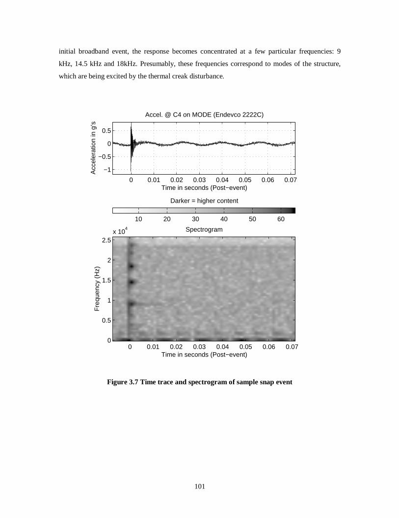
101

initial broadband event, the response becomes concentrated at a few particular frequencies: 9

kHz, 14.5 kHz and 18kHz. Presumably, these frequencies correspond to modes of the structure,

which are being excited by the thermal creak disturbance.

0 0.01 0.02 0.03 0.04 0.05 0.06 0.07

−1

−0.5

0

0.5

Accel. @ C4 on MODE (Endevco 2222C)

Time in seconds (Post−event)

Acc

eler

atio

n in

g’s

Spectrogram


Fre

quen

cy (

Hz)

0 0.01 0.02 0.03 0.04 0.05 0.06 0.070

0.5

1

1.5

2

2.5x 10

4

Darker = higher content

10 20 30 40 50 60

Figure 3.7 Time trace and spectrogram of sample snap event

102

−1 0 1 2

x 10−3

−1

−0.5

0

0.5

Event Transient (256 pts)

Time (sec)

Acc

el. (

g)

103

104

10−10

10−8

10−6

10−4

PSD (single window)

Freq. (Hz)

Mag

n. (

g2 /Hz)

−7 −6 −5 −4

x 10−3

−1

−0.5

0

0.5

Pre−event Vibr. (256 pts)

Time (sec)

Acc

el. (

g)

103

104

10−10

10−8

10−6

10−4

PSD (single window)

Freq. (Hz)

Mag

n. (

g2 /Hz)

Figure 3.8 Truncated sample data (256-point windows)

An alternative way to perform the frequency-domain characterization would be to compute the

PSD of the event transient. Rather than computing the PSD based on the full time trace, of which

the event may only represent a small fraction, the data can be truncated to focus on the snap

event. Proper selection of the window is important, as the Fourier analysis via PSD is rather

sensitive to the windowing process: choosing too large a window, or not centering it around the

event transient results in inaccurate representation of the modal content of the signal. The two

plots on the left-hand side of Figure 3.8 show the truncated data and the corresponding PSD; a

single 256-point Hanning window was convolved with the time trace shown, prior to computing

the spectrum. For comparison purposes, a 256-point time trace of the pre-event vibration is

presented on the right-hand side of Figure 3.8, along with the corresponding PSD. The

differences between the two PSDs represent the frequency content of the response to the thermal

snap disturbance. The PSD of the event transient is generally higher than that of the pre-event

response; this is an indication of the broadband nature of the disturbance. The peaks in the left-

hand side PSD represent the particular frequencies at which truss response was excited. The same

structural modes are evident as in the spectrogram, located around 9 kHz, 14.5 kHz and 18kHz. In

general, however, frequency-domain characterization via PSD analysis does not provide

103

information on time-varying frequency content as effectively as the spectrogram, so the latter

technique will be used to analyze the results from the bulk of the thermal snap tests.

A time-domain characterization of the event can also provide valuable information on the

frequency content and damping of the transient vibration. Figure 3.9 shows a zoomed-in view of

the sample event transient. The multi-mode nature of the transient vibration, which was shown in

the frequency-domain analysis, is also evident in this time trace. In order to extract the portion of

the response due to a particular mode of the truss, a narrow bandpass filter can be used. The

middle plot of Figure 3.9 shows the transfer function characteristics of an eighth-order bandpass

Butterworth filter, with pass-band between 8800 Hz and 9200 Hz. Since the filtering is being

performed on the data during post-processing (i.e. the full data trace is available), a non-causal

filtering technique can be used to eliminate phase distortions in the filtered response. The

resulting filtered signal corresponds to the truss response at the 9 kHz mode, and is shown in the

bottom plot of Figure 3.9. While some signal amplitude may be lost due to the filtering process,

and some startup transients may be present, this filtered signal should nonetheless be a fairly good

approximation to the true 9 kHz mode response, particularly once the startup transients have died

out.

The modal damping can be estimated, by fitting an expression for an exponentially-decaying

sinusoidal function to a truncated portion of the filtered trace. This simple SDOF time-domain

technique is based on the assumption that the free decay response of a single-mode system is

given by:

)sin( φωζω += − tAey t

where ζ is the modal damping ratio (a viscous damping model is assumed), ω is the frequency of

the mode, φ is the initial phase angle, and A is a scaling amplitude factor. Figure 3.10 shows a

truncated portion of the filtered signal, overlaid with the exponentially-decaying sinusoid fit.

Clearly, the fit does a reasonably good job of representing the filtered signal; however, after the

1.5 millisecond point, the filtered signal becomes more heavily damped than the fit. This may

indicate that another damping mechanism takes over once the amplitude of oscillation gets small

enough, which cannot be accurately modeled using a single-mode decay. The value of the ζ

obtained from this fit is roughly 2%. It should be noted that this damping estimate would include

the effect of any apparent damping which might be occurring, due to energy transfer to other

104

modes [13]. Nonetheless, such a ζ value is consistent with the level of damping expected in a

high-frequency local mode of a jointed structure made of Lexan and aluminum.

In summary, various time- and frequency-domain characterization techniques have been

demonstrated here on the sample data trace. These are the methods which will be used to analyze

the results from the thermal snap experiment, to be presented in section 3.4.

0 0.5 1 1.5 2 2.5 3 3.5

x 10−3

−1

−0.5

0

0.5

Accel. @ C4 on MODE (Endevco 2222C)

Time (seconds, post−event)

Acc

el. (

g)

103

104

105

10−10

100

8th Order Butterworth Bandpass Filter

Frequency (Hz)

Mag

nitu

de

0 0.5 1 1.5 2 2.5 3 3.5

x 10−3

−0.1

0

0.1

Filtered Accel. Data

Time (seconds, post−event)

Acc

el. (

filte

red

g’s)

Figure 3.9 Truncated and filtered transient event data

105

0 0.5 1 1.5 2 2.5

x 10−3

−0.015

−0.01

−0.005

0

0.005

0.01

0.015Filtered Accel. Ring−down with Fit to Trace

Time (s)

Acc

el. (

g)

fit signal

Figure 3.10 Exponentially-decaying sinusoid fit to filtered event

3.3 Measures Taken to Identify Thermal Snap

In an investigation of this kind, great care must be taken to ensure that vibration events due to the

phenomenon of interest – thermal snap, in this case – can be identified as such. This section

highlights the recognizable characteristics of thermal snap events, and documents the different

measures taken to distinguish events due to thermally-induced structural vibrations from events

due to other sources.

Although a review of the existing literature has turned up very few actual observations of the

phenomenon, certain expected characteristics of thermal creak can be identified, through

knowledge of a structure and its frictional mechanisms, combined with simple models of the

disturbance, such as those developed by Kim [27]. Thermal creak only occurs once a critical level

of internal stress is reached in an indeterminate structure; the creak event is therefore expected to

occur sometime during a temperature transient, after stress has built up over some time, but

before steady-state has been attained. It should be noted, however, that temperature

measurements taken on the surface of the structure do not necessarily reflect the mean

temperature distribution internal to the structure: some amount of temperature lag between the

internal temperature of the structure and the surface temperature is unavoidable. The extent of

this lag is dependent on the thermal mass and conductivity of the material. For instance, even

though the temperature may have reached steady-state on the surface of a Lexan batten member

in the deployable module, internal stress may still be building up inside the member, because the

106

internal temperature of the strut may still be changing. Correlating the time of occurrence of an

event and the temperature state of the structure at that instant should provide a first indication of

the likelihood that an observed event is due to thermal snap. Another indication is provided by the

time- and frequency-domain analyses of the event signal. Since thermal snap is an impulsive (i.e.

broadband) structural disturbance, the time trace and frequency spectrum should reflect the

telltale signs of structural response: multi-modal, lightly-damped harmonic vibration.

With the “expected” characteristics of the phenomenon of interest identified, the next step is to

identify all of the non-thermally-induced disturbance sources in the tests. If these sources can be

eliminated, or if the signals caused by these sources can be distinguished from those caused by

thermal creak, then it ensures that the objectives of this investigation (demonstration and

characterization of thermal snap) can be met. The different possible non-thermally-induced

disturbances can be listed as follows, based on the test conditions encountered:

− aerodynamic buffeting of the suspended truss;

− vibrations transmitted through the suspension system, or sensor wires;

− incidental contact with the structure (by wires, umbilical connector, debris);

− acoustic excitation of the structure (from noisy pumps, compressors, fans);

− electrical events picked up by the sensors or wiring;

− excitation of accelerometer resonances.

These disturbance sources are described below, along with the various measures taken to

mitigate, or at least identify, each of them.

Aerodynamic buffeting

During the tests performed in the convection thermal chamber, the deployable module

experienced noticeable aerodynamic buffeting, as a result of the turbulent air being circulated

through the chamber by the fans. The bouncing of the truss on its suspension springs was visible

through a window on the chamber door. The roll-off of the suspension system caused this

disturbance to only affect low-frequency vibration, as evidenced in the autospectrum of the

background noise in Figure 3.3. Since the hunt for thermal snaps focused on frequencies above 1

kHz, this disturbance could not be confused with potential snap events. However, the constant

motion of the structure may have significantly affected the observed snap behavior. It is

conceivable that by constantly dithering the frictional joints in the structure, the amplitude and

107

frequency of occurrence of thermal snaps may be different than would be for a completely

stationary truss. This dithering effect is identified as a likely reason why snap events were much

more globally observable in the convection tests, compared to the radiation tests (see section 3.4).

Transmission of mechanical vibrations

The thermal chambers provide a significant background vibration environment, due to the various

heaters, pumps and compressors they employ. During the tests, transmission of these vibrations to

the truss could only occur through the suspension springs, or the various sensor wires running

from the truss to the chamber walls. A number of measures were in place to eliminate as much of

the transmitted disturbance as possible. First of all, the roll-off of the suspension system would

greatly attenuate any chamber vibration, particularly in the high-frequency range of interest. Also,

care was taken to keep enough slack in the accelerometer cables and thermocouple wires leading

off the structure to avoid an accidental load path. In addition to these two attenuating effects,

extra precautions were put in place to identify any chamber-induced vibration, should it somehow

be detectable on the truss. Accelerometers were always mounted at either end of one suspension

spring (on the chamber ceiling and the truss corner fitting), in order to correlate any structural

vibrations with chamber vibrations. In addition, for a number of the convection tests, the dummy

truss bay described in subsection 3.1.1 was suspended next to the deployable truss and

instrumented with accelerometers; a true thermal snap would only be detected on the deployable

truss, and not on the dummy.

Incidental contact

For tests performed in the convection chamber, there was concern that the blowing air might

cause debris, or perhaps a wire or the umbilical connector to impact the truss, causing a response

which might be difficult to discern from a thermal snap event. For this reason, a few measures

were implemented to eliminate this possibility. The chamber was thoroughly cleaned before each

test, so that all debris large enough to cause a significant impact was removed. The sensor wires

were taped off the structure in such a way that they would not be able to contact it (yet still

remained slack enough to prevent a load path to the structure). As for the heavy umbilical

connector, an elastic cord was used to “isolate” it and keep it separated from the truss, in much

the same way as in the microdynamic modal parameter characterization experiment (see

108

discussion in section 2.3 and photo in Figure 2.24). In addition, the umbilical was completely

removed for the final tests performed at Lincoln Laboratory.

Acoustic excitation

Unlike the microdynamic modal parameter characterization experiment discussed in Chapter 2,

the frequency range of interest for the thermal snap tests was high enough that acoustic

transmission of disturbances through the air became a concern. By performing tests in an

evacuated chamber at Lincoln Laboratory, this disturbance source was eliminated. For the tests

performed in the convection chamber, the instrumented dummy structure provided a means of

distinguishing between acoustic and thermal creak disturbances: acoustic excitation should affect

the dummy and deployable trusses similarly.

Electrical events

Another type of disturbance, which was of concern in both the radiation and convection tests, was

the pick-up of electrical signals by the sensors or their wiring. Electrical disturbances were

unavoidable in an experiment of this type; the data acquisition system was susceptible to “false”

triggering, due to electrical events, such as those associated with activation of valves or pumps

from the chamber. The accelerometer signals were even sensitive to the cross-talk generated by

switching the thermocouple being read on the Omega digital thermometer.

Although electrical disturbances could not be eliminated, they were fairly easy to identify,

fortunately. They were evident as very sharp spikes in the data, which exhibited very little of the

exponentially-decaying ringing one would expect from a structural disturbance. Figure 3.11

shows an example of an event identified as electrical in origin. On the time trace, the event

appears as a very sharp impulse; this translates to a short-duration broadband frequency response

visible on the spectrogram. However, no structural ringing or multi-mode behavior is excited,

distinguishing this type of event from a thermal creak.

Accelerometer resonance excitation

Another possible, although unlikely, source of disturbance is the excitation of an Endevco

7265A-HS accelerometer resonance, perhaps due to internal stiction within the sensor, at

109

temperatures exceeding its operating range (which could be thought of as “thermal snap” inside

the accelerometer). However, should this type of excitation occur, it would be easily identifiable

as a single-mode, highly-damped resonance (the fn and ζ specifications for these accelerometers

are ~1400 Hz and 70%, respectively). Furthermore, all of the 7265A-HS accelerometers were

removed with the umbilical cable, for several tests performed in the radiation chamber. The

2222C accelerometers were then exclusively used as the sensors for snap detection.

0 0.01 0.02 0.03 0.04 0.05 0.06 0.070

0.05

0.1

Accel. @ A1 (Endevco 7265−HS)

Time in seconds (Post−Event)

Acc

eler

atio

n in

g’s


Fre

quen

cy (

Hz)

Spectrogram

Color scale for freq content in dB

0 0.01 0.02 0.03 0.04 0.05 0.06 0.070

0.5

1

1.5

2

2.5x 10

4

−120 −100 −80 −60 −40 −20

Figure 3.11 Sample electrical event

110

3.4 Experimental Results

In this section, the results from the thermal creak investigation are presented. Aside from the

thermal tests performed at Payload Systems, Inc. and MIT Lincoln Laboratory, a simple series of

tap tests was performed, in order to spatially characterize the truss response to an impulsive

disturbance. The results from this preliminary tap test are discussed in subsection 3.4.1, followed

by the results from the convection and radiation tests, in subsections 3.4.2 and 3.4.3, respectively.

Finally, in subsection 3.4.4, the findings of the investigation will be summarized, based on the

ensemble of test results.

3.4.1 Tap Test Results

When an impulsive disturbance like thermal snap occurs, its effects are felt differently across the

structure, depending on various factors, such as materials, size and shape of the structural

elements, mechanisms in the disturbance transmission path, etc… For instance, the magnitude

and frequency content of the transient response may be different, from measurements taken at

different locations on the structure. Time lags in the onset of the event may be evident between

different sensor locations, illustrating the speed of propagation of the disturbance through the

structure. Some disturbances may be impeded strongly enough as they progress through the

structure, such that they are unobservable from certain locations.

The wave propagation of disturbances through periodic lattice structures, like the deployable truss

considered here, has been studied by numerous researchers [45, 46]; a full wave propagation

analysis of the thermal snap response is outside the scope of this work. However, a simple

experimental investigation can provide considerable insight into the spatial response to an

impulsive disturbance. In order to simulate thermal snap disturbances, the suspended structure

was tapped at different joint locations with a steel instrument. Even though the nature of the

disturbance thus applied to the truss is not internal to a joint, like the slip of a frictional interface

would be, it nonetheless results in a broadband, impulsive excitation, traceable to thermal creak.

Using the same sensors and data acquisition system as the thermal tests, the response to the taps

can be observed at selected locations on the truss. In this subsection, typical results from this

series of tests are discussed, followed by a summary of the relevant response characteristics.

111

Representative tap test data is presented in Figures 3.13 and 3.14. Each of these two figures

shows the truss response at two different locations, in response to a given tap location. The

sensors used for these tests were Endevco 2222C accelerometers; their locations and sensing

directions are illustrated in Figure 3.12. These sensor locations correspond to a subset of those

used in the thermal tests performed at Lincoln Laboratory, on November 25th, 1997 (see

subsection 3.4.3). Figure 3.12 also shows the locations and directions of the two tap disturbances.

The sensor and tap locations were limited to a single bay, in order to focus the investigation on

local phenomena, which were the most likely to be observed during the thermal snap tests, as

explained in subsection 3.1.3.

Tap #1 was applied transversely to a knee joint, on a neighboring longeron to the one

instrumented with sensors C1 and C2. Figure 3.13 shows the response time traces at both

accelerometer locations, as well as spectrograms highlighting the time-varying frequency content

of each signal. Both traces show somewhat similar behavior: initial high-frequency vibration

which dies out rapidly, superposed with lower-frequency oscillations which persist through to the

end of the trace. By zooming in on the two traces, no discernable difference is evident between

the event start times, indicating that the disturbance from the tap propagates to both

accelerometers in roughly the same amount of time. The broadband nature of the impulsive

disturbance is evident in the spectrogram plots – dark horizontal streaks represent the multi-

modal response of the structure. The streaks at low frequencies are longer than those at higher

frequencies, evidence of the shorter time constants associated with higher structural modes.

Though the maximum amplitudes of vibration attained are comparable for C1 and C2, the initial

high-frequency transient is stronger at C2; this may be evidence of local modes within the batten

frame corner fitting, which would occur at higher frequencies than the dominant local modes of

the longeron. It may also indicate that the axially-oriented accelerometer at C2 is picking up axial

modes of vibration of the longeron struts, which would not be observable from the transverse-

sensing accelerometer at C1.

The second tap location was collocated with accelerometer C2. Figure 3.14 shows the response to

this disturbance, again in the form of a time trace and spectrogram, as observed from C1 and C2.

Three impulsive events are visible in the time traces, due to “rebound” of the tapping instrument

during the tap process. Again, the broadband nature of the disturbance is seen in both

spectrograms. However, this time the modal response is much stronger at high frequencies; unlike

the response to Tap #1, no low-frequency oscillations are evident in the time traces. The

112

exponential decay of the high-frequency transient is particularly clear in the response at C2: it

would appear that the response measurement collocated with the impulsive disturbance is

dominated by the high-frequency local dynamics directly excited by the impulse. Not

surprisingly, the magnitude of vibration is much higher at the tap-collocated sensor. In addition,

the event is picked up approximately 0.1 millisecond earlier at C2 than at C1, representing the

wave propagation time required for the disturbance to travel halfway down the Lexan longeron.

The observations drawn from the series of tap tests can be summarized as follows:

− the event start times and the amplitudes of vibration depend on the distance from the

disturbance source, and the sensing direction of the accelerometers (as expected, the event

occurs sooner, and the response amplitude is higher, for a sensor collocated and aligned with

the disturbance);

− the vibration response near the disturbance source is dominated by high-frequency, “local”

transients;

− for sensors far enough away from the source (along the load path), the only evidence of the

event is low-frequency response, as energy leaks into more “globally-acting” modes of the

structure.

C1

C2

Tap #1

Tap #2

Figure 3.12 Sensor and tap locations for tap tests

113

0 0.02 0.04 0.06−2

0

2

Accel. @ C1 (Tap #1)

Time (s)

Acc

el (

g)

Time (s)

Fre

q (H

z)

Spectrogram


0 0.02 0.04 0.060

1

2

x 104

−40 −20 0 20

0 0.02 0.04 0.06

−1012


Time (s)

Acc

el (

g)

Time (s)

Fre

q (H

z)

Spectrogram


0 0.02 0.04 0.060

1

2

x 104

−80 −60 −40 −20 0 20

Figure 3.13 Response to Tap #1

0 0.02 0.04 0.06

−5

0

5


Time (s)

Acc

el (

g)

Time (s)

Fre

q (H

z)

Spectrogram


0 0.02 0.04 0.060

1

2

x 104

−60 −40 −20 0 20

0 0.02 0.04 0.06−20

0

20


Time (s)

Acc

el (

g)

Time (s)

Fre

q (H

z)

Spectrogram


0 0.02 0.04 0.060

1

2

x 104

−40 −20 0 20 40

Figure 3.14 Response to Tap #2

114

3.4.2 Convection Test Results

Between May 22nd and September 2nd, 1997, thermal tests were performed on the MODE

deployable module in the convection chamber at Payload Systems, Inc. These tests yielded a

number of events which were identified as thermal creak, based on arguments presented in

section 3.3. In this subsection, discussion will focus on two representative events in particular,

which exhibit characteristics typical of the events observed during the convection tests. One

typical event is chosen from among those recorded during the test performed on June 23rd, while

the other is chosen from the results of the September 2nd thermal test. For both of these events, the

results from the time- and frequency-domain analyses are presented and discussed.

Figure 3.15 shows the temperature profiles from the June 23rd test; the temperature data was

obtained from the thermocouples, placed at various locations on the deployable truss and in the

chamber. The locations of these thermocouples are indicated by triangles on the sensor map of

Figure 3.16. Three of these thermocouples, labeled T5, T7 and T8, were attached to different

parts of the truss structure: a Lexan batten, an aluminum batten frame corner fitting and a steel

diagonal cable. A fourth thermocouple (T9) was attached off the chamber ceiling, to measure the

ambient temperature in the chamber. As evident in Figure 3.15, the three truss temperature

profiles follow the ambient temperature profile quite closely, indicating that the convection heat

transfer process results in rapid equilibration of the surface temperatures across the test article

with the ambient temperature.

For the June 23rd test, only the deployable truss was suspended in the thermal chamber; the

dummy truss bay was not used. The sensor location diagram in Figure 3.16 shows the placement

and orientation of the accelerometers used to detect thermal snap events, for this set of tests.

Throughout this chapter, a consistent labeling code is used to discriminate between the various

types of sensors: each sensor is identified by a letter and number, corresponding to the sensor

type and location, respectively. The labels for the 7265A-HS accelerometers all begin with the

letter “A”; the 2222C accelerometers are identified with the letter “C”; the strain gauges, with the

letter “S”; and finally, the thermocouples, with the letter “T”. For instance, the Model 2222C

accelerometer placed on the ceiling of the thermal chamber, near the attachment point of one of

the suspension springs, is labeled C1. Another 2222C sensor, labeled C2, is located on the

deployable truss, at the base of the same suspension spring. Two Model 7265A-HS

115

accelerometers are given the tags A2 and A4. As mentioned above, the four thermocouples on the

diagram are identified as T5, T7, T8 and T9.

0 50 100 150 200 250−30

−20

−10

0

10

20

30

40


Time (min)

Tem

pera

ture

(de

g C

)

1 2

T5T7T8T9

Figure 3.15 Temperature profile for typical convection test (June 23, 1997)

A2

C1

C2

T5T7

T8

T9 (ambient)

A4

Figure 3.16 Sensor distribution for typical convection test (June 23, 1997)

116

0 0.02 0.04 0.06−1

0

1Time Trace for Accel @ C1

Time (s)

Acc

el (

g)

Time (s)

Fre

q (H

z)

Spectrogram


0 0.02 0.04 0.060

1

2

x 104

−60 −40 −20 0 20

0 0.02 0.04 0.06−1

0


Time (s)

Acc

el (

g)

Time (s)

Fre

q (H

z)

Spectrogram


0 0.02 0.04 0.060

1

2

x 104

−80 −60 −40 −20 0

0 0.02 0.04 0.06−0.04−0.02

00.020.040.06

Time Trace for Accel @ A4

Time (s)

Acc

el (

g)

Time (s)

Fre

q (H

z)

Spectrogram


0 0.02 0.04 0.060

1

2

x 104

−100 −80 −60 −40 −20 0

Figure 3.17 Thermal snap data from typical convection test (June 23, 1997)

117

The first typical event to be discussed here was detected during the cooling phase of the second

thermal cycle, after approximately 185 minutes had elapsed since the start of the June 23rd test.

This event is identified by the vertical dashed line labeled “2”, in the temperature profile diagram

(Figure 3.15). One Tektronix Model 2630 data acquisition unit was used to record the typical

event as observed from three accelerometer sensors (C1, C2, and A4). Accelerometer A2 was not

connected to the fourth channel of the data acquisition unit at the time the event occurred. The

nominal bandwidth setting of 20 kHz was chosen, resulting in a sampling frequency of 51200 Hz

and time traces of 0.08 second duration, of which 0.008 second corresponds to pre-event data.

The time traces and spectrograms of the event as measured on the three accelerometers are

presented in Figure 3.17. Looking at the three time traces, it is evident that the impulsive event

picked up by the two accelerometers on the test article (C2 and A4) is not visible in the trace from

the accelerometer attached to the chamber ceiling (C1). Furthermore, the broadband frequency

content seen at time zero in the spectrograms for signals C2 and A4 is not present in the plot for

signal C1, confirming that the impulsive event was felt on the deployable truss, but not on the

chamber ceiling. One of the conclusions drawn from the tap tests (see subsection 3.4.1) was that

high-frequency transients dominate the vibration response in close proximity of the disturbance

source. Judging by the dominance of the high-frequency transient behavior in both signals C2 and

A4, it is reasonable to deduce that the snap occurred near those accelerometer locations.

Both accelerometers on the truss show frequency content in the disturbance up to greater than 20

kHz. However, the spectrogram plot reveals that significant content of the A4 signal is found in

frequencies below 2 kHz. This is most likely due to the roll-off of the Model 7265A-HS

accelerometer (as mentioned in section 3.3, these sensors have a heavily-damped resonance

around 1400 Hz). The darker spots in the content band around time zero correspond to modal

content in the response transients. In particular, strong modal content around 6 kHz is evident in

both the C2 and A4 data. Because these two sensors are located reasonably close to one another

and share the same line of action, it is not surprising to see common modal content in the event

transient signals. The different frequency response characteristics of the 2222C and 7265A-HS

accelerometers make comparison between the magnitudes of the C2 and A4 acceleration traces

difficult. Accelerometer A4 has a much lower bandwidth, and consequently, the higher-frequency

(and thus higher-amplitude) content is being significantly attenuated. This effect is certainly the

main reason why the maximum acceleration level of 1 g attained in the C2 trace is more than an

order of magnitude greater than that reached in the A4 trace. Hence, looking at the response

118

amplitude provides no clue as to which of the two accelerometers is nearest to the source of the

disturbance. Zooming in on the time traces, however, it is observed that the event starts 0.2 ms

sooner at C2 than at A4, suggesting that C2 is “closest” to the source, along the wave propagation

path provided by the structure.

By filtering both traces as described in section 3.2, the exponential ring-down of the 6 kHz mode

can be obtained; fits to both filtered signals yield a damping ratio of 0.5%, a realistic value for

structural damping. This provides further evidence that the disturbance is structural in nature, and

is not due to electrical cross-talk. The source of this disturbance is deduced to be thermal snap, as

opposed to an acoustic disturbance: an acoustic event capable of generating such significant

response on the truss would have been unlikely to go unnoticed (i.e. unheard, or undetected by

accelerometer C1) during the test. In order to confirm this deduction, other thermal tests were

performed with the dummy truss bay suspended next to the deployable module; the second

typical snap event to be discussed was recorded during one such test.

0 50 100 150 200−30

−20

−10

0

10

20

30

40

50Temperature Profiles for Convection Test (Sept 2, 1997)

Time (min)

Tem

pera

ture

(de

g C

)

1 2

T1T2

Figure 3.18 Temperature profile for typical convection test (September 2, 1997)

119

For the test performed on September 2nd, the temperature profiles are plotted in Figure 3.18. This

time, only two thermocouples were used: one to keep track of the surface temperature on the test

article (T1), and another to measure the ambient temperature in the convection chamber (T2). As

expected, no significant difference is noted between the two measured temperatures, at any time

during the test. Figure 3.19 shows the sensor distribution across the deployable truss and dummy

truss bay. Five accelerometers were used to detect thermal snaps on the deployable module (C2,

C3, C4, A1 and A6). As for the June 23rd test, one accelerometer (C1) was placed on the chamber

ceiling, at the base of one of the springs. Finally, the dummy bay was instrumented with two

more accelerometers (C5 and C6).

C1

C2C3

C4

A1

A6

C5

C6

T1

T2 (ambient)

Figure 3.19 Sensor distribution for typical convection test (September 2, 1997)

120

0 0.02 0.04 0.06

−0.50

0.5

Time Trace for Accel @ C1

Time (s)

Acc

el (

g)

Time (s)

Fre

q (H

z)

Spectrogram


0 0.02 0.04 0.060

1

2

x 104

−80 −60 −40 −20 0 20

0 0.02 0.04 0.06

−0.2

0

0.2Time Trace for Accel @ C2

Time (s)

Acc

el (

g)

Time (s)

Fre

q (H

z)

Spectrogram


0 0.02 0.04 0.060

1

2

x 104

−80 −60 −40 −20 0

0 0.02 0.04 0.06

−1−0.5

00.5


Time (s)

Acc

el (

g)

Time (s)

Fre

q (H

z)

Spectrogram


0 0.02 0.04 0.060

1

2

x 104

−60 −40 −20 0 20

0 0.02 0.04 0.06−0.05

0

0.05


Time (s)

Acc

el (

g)

Time (s)

Fre

q (H

z)

Spectrogram


0 0.02 0.04 0.060

1

2

x 104

−100 −80 −60 −40 −20 0

Figure 3.20a Thermal snap data from typical convection test (September 2, 1997)

121

0 0.02 0.04 0.06

−0.5

0

0.5


Time (s)

Acc

el (

g)

Time (s)

Fre

q (H

z)

Spectrogram


0 0.02 0.04 0.060

1

2

x 104

−80 −60 −40 −20 0 20

0 0.02 0.04 0.06−0.04−0.02

00.020.040.060.08


Time (s)

Acc

el (

g)

Time (s)

Fre

q (H

z)

Spectrogram


0 0.02 0.04 0.060

1

2

x 104

−80 −60 −40 −20 0

0 0.02 0.04 0.06

−0.050

0.05


Time (s)

Acc

el (

g)

Time (s)

Fre

q (H

z)

Spectrogram


0 0.02 0.04 0.060

1

2

x 104

−80 −60 −40 −20 0

0 0.02 0.04 0.06

−0.10

0.10.2


Time (s)

Acc

el (

g)

Time (s)

Fre

q (H

z)

Spectrogram


0 0.02 0.04 0.060

1

2

x 104

−100 −80 −60 −40 −20 0

Figure 3.20b Thermal snap data from typical convection test (September 2, 1997)

122

During the September 2nd test, a number of events identified as thermal snaps were recorded, as

indicated by the vertical dashed lines on the temperature profile plot. Of these, one is presented

here as the second typical snap event for the convection tests. The chosen event occurred

approximately 180 minutes into the test, and is identified as event “2” in Figure 3.18. In order to

record the snap, two Model 2630 data acquisition units were used. Both were set to 20 kHz

bandwidth. Accelerometers C1, C2, C3 and A6 were connected to the channels on one unit, while

C4, C5, C6 and A1 were hooked up to the second unit. It should be noted that these two units

were triggered independently from each other, so the time scales for channels on different units

do not overlay exactly (i.e. comparison cannot be made between the event start times for signals

captured on different data acquisition units).

Figures 3.20a and 3.20b present the time traces and spectrograms corresponding to the typical

event. No sign of the event was seen in the signals from the accelerometers on the chamber

ceiling and the dummy truss (C1, C5 and C6), even though evidence of an impulsive disturbance

was clearly observed by all the sensors on the deployable truss (C2, C3, C4, A1 and A6). Based

on the time traces from the accelerometers on the deployable truss, and the insight acquired from

the tap tests, it appears that the thermal snap occurred roughly midway along the length of the

truss, in the vicinity of C3 and C4 (see Figure 3.19). These two traces exhibit the highest-

amplitude transients (maximum amplitudes greater than 0.5 g), and are the signals most

dominated by high-frequency response, as expected in proximity of the disturbance source

(although neither signal shows the same level of high-frequency dominance as the C2 signal from

the June 23rd typical event). A comparison between the start times of the event as measured by

sensors C2, C3 and A6 (all connected to the first Tektronix data acquisition unit) supports the

deduction that the event occurred near C3: zooming in on the traces reveals that the event began

0.7 millisecond later at C2 and A6 than at C3. However, no discernable time lag is seen between

the event start times on C4 and A1, which were hooked up to the second Tektronix unit.

Accelerometer A1 shows more high-frequency content than C2 and A6, suggesting that the snap

acted predominantly in the horizontal, transverse direction with respect to the deployable truss (in

the sensing direction of A1, C3 and C4, perpendicular to the sensing directions of C2 and A6).

As far as frequency content of the response is concerned, the C3, C4, and A1 spectrograms show

that various modes between 10 kHz and 23 kHz were excited by the snap; in general, the dark

spots occur at different frequencies for different sensors, indicating that these high-frequency

modes are predominantly local. In particular, the C3 trace shows strong modal response around

123

10.5 kHz in the initial transient. The filtering and fitting process described in section 3.2 results in

a damping ratio of approximately 1% for this mode, a reasonable value for structural damping.

Although the poor resolution of the spectrograms makes it difficult to accurately characterize the

low-frequency content, it is evident that all the accelerometers on the deployable truss picked up

significant response below 2 kHz or so.

It should be noted that this typical event was fifth in the sequence of events picked up during the

second cooling phase of the September 2nd thermal test (see Figure 3.18). All of these sequential

events looked very much alike, in terms of the “shape” and frequency content of the response

time traces, except that the overall magnitude of response seemed to decrease with each

successive event. Additionally, each pair of successive snaps exhibited the trend of increasing

separation in time. This type of behavior points to the possibility of repeated creaking of one slip

interface over the temperature transient, with increasing time intervals between slips as the

structure approached steady-state temperature. Thus, even in a nominally symmetric and repeated

structure like the deployable module, some joints are more “at risk” than others for experiencing

thermal creak, perhaps due to differences in the friction parameters at the interface, or slight

asymmetries in the internal stress distribution. Similar successive impulsive disturbances,

exhibiting the general trends of decreasing amplitude and increasing time separation, were

observed on the Hubble Space Telescope during its initial on-orbit checkout; these impulsive

events, which occurred during the orbital “day”, were attributed to thermal creak in the solar

array spreader bars [26].

In summary, results from the time- and frequency-domain analyses performed on two typical

thermal snap events from the thermal convection tests have been presented and discussed. The

accelerometer response data from these two sample snaps exhibited certain characteristics which

were representative of the ensemble of convection test results:

- the events were all seen as impulsive, broadband disturbances;

- the response to every event was observed across the entire deployable structure;

- the response was multi-modal in nature;

- the response exhibited significant modal content at frequencies below 2 kHz;

- the varying magnitude and frequency content of the response across the truss permitted some

degree of spatial localization of the event.

124

3.4.3 Radiation Test Results

In order to eliminate the aerodynamic buffeting and acoustic disturbance sources present in the

convection tests, a series of thermal snap investigations was performed in a vacuum chamber,

using radiation as the mechanism for heat transfer to the deployable truss. This also allowed for a

more realistic simulation of the orbital environment which would be encountered by a space

structure. As described in subsection 3.1.2, a thermal vacuum chamber at MIT Lincoln

Laboratory was the site of the radiation tests, between September 29th and November 26th, 1997.

During these tests, several events were identified as thermal snaps. In this subsection, two

representative events are selected to illustrate the typical characteristics of the snaps from the

radiation tests. The first thermal creak to be discussed here occurred on September 29th, during

the first radiation test; the second was observed on November 25th. As was done for the typical

convection results, the time- and frequency-domain analyses of these two representative snaps are

discussed below.

Figure 3.21 shows the temperature profiles for the September 29th test. Although eight

thermocouples were placed on the structure and shroud during the test, only five of the

temperature traces are plotted in the profile, for clarity. As shown in the sensor map of Figure

3.22, thermocouples T2 and T3 were bonded to one of the longerons, on a Lexan strut and an

aluminum joint, respectively, while thermocouple T6 was attached to a Lexan batten member.

Sensors T7 and T8 were used to measure the temperatures on the radiation shroud, at the bottom

and top, respectively. In order to simulate a sudden, significant thermal load, such as would be

encountered by a spacecraft entering or exiting planetary eclipse, an “impulsive” thermal load

was applied to the test article. The lowest truss temperature was measured on the Lexan batten

(T6), which dropped to just under –25°C after approximately 50 minutes.

For this test, four Model 2222C accelerometers were used to detect structural events (see Figure

3.22). Sensor C1 was placed on the top of the shroud, at the attachment point for one suspension

wire and spring. Accelerometer C2 was bonded to the aluminum corner fitting on the deployable

module, at the other end of the same spring. The other two accelerometers, C3 and C4, were

attached to aluminum joints on two different longerons.

125

0 20 40 60 80 100 120−200

−150

−100

−50

0


Time (min)

Tem

pera

ture

(de

g C

)

1

T2T3T6T7T8

Figure 3.21 Temperature profiles from typical radiation test (September 29,1997)

C1

C2C3

C4

T8 (top of shroud)

T2

T3

T1

T7 (bottom of shroud)

T4

T5

T6

Figure 3.22 Sensor distribution for typical radiation test (September 29, 1997)

126

0 0.02 0.04 0.06−0.2−0.1

00.1


Time (s)

Acc

el (

g)

Time (s)

Fre

q (H

z)

Spectrogram


0 0.02 0.04 0.060

1

2

x 104

−80 −60 −40 −20 0

0 0.02 0.04 0.06

−0.2

−0.1


Time (s)

Acc

el (

g)

Time (s)

Fre

q (H

z)

Spectrogram


0 0.02 0.04 0.060

1

2

x 104

−40 −20 0 20

0 0.02 0.04 0.06

−0.3−0.2−0.1

00.1


Time (s)

Acc

el (

g)

Time (s)

Fre

q (H

z)

Spectrogram


0 0.02 0.04 0.060

1

2

x 104

−80 −60 −40 −20 0

0 0.02 0.04 0.06−1

−0.50

0.5


Time (s)

Acc

el (

g)

Time (s)

Fre

q (H

z)

Spectrogram


0 0.02 0.04 0.060

1

2

x 104

−80 −60 −40 −20 0

Figure 3.23 Thermal snap data from typical radiation test (September 29, 1997)

127

During the September 29th test, one event was identified as thermal creak. It occurred

approximately 43 minutes into the test, as indicated by the vertical dashed line in Figure 3.21.

One Tektronix Model 2630 unit (set to a bandwidth of 20 kHz) was used to record the

accelerometer data resulting from the event. Figure 3.23 contains the time traces and

spectrograms from the four channels. The oscillatory signal evident in all four traces is actually

electrical line noise at 60 Hz, which was picked up by the sensor wires. As expected for a thermal

creak occurring on the test article, the trace from the accelerometer placed on the shroud (C1)

shows no sign of the event. Unlike the events recorded during the convection tests, only one

accelerometer on the truss detected the broadband snap: the impulsive event with peak amplitude

around 1 g is clearly evident in the trace from accelerometer C4. Another important difference

between this event and those from the convection tests is that the post-event frequency content is

not concentrated at frequencies below 2 kHz; rather, the energy in the response is focused at

higher frequencies. Evidently, the response to the snap was only felt in high-frequency modes,

localized in the vicinity of accelerometer C4.

The time- and frequency-domain analysis of the event in the C4 trace has already been performed

in section 3.2, in order to illustrate the data reduction procedure. This analysis identified the

broadband nature of the disturbance, and the three dominant modes of response at 9 kHz, 14.5

kHz and 18kHz. Truncating and bandpass filtering the trace around the 9000 Hz mode allowed

the modal damping ratio to be estimated at around 2%, a reasonable level of damping for a local

mode in a jointed structure predominantly made of Lexan. The damping estimates for the other

two dominant modes yield values between 1% and 2%, as well.

The second typical snap event to be discussed here was observed during the November 25th

thermal test. The temperature profiles are plotted in Figure 3.24, and the sensor distribution is

given in Figure 3.25. For this test, the sensors on the deployable truss were clustered in two

groups, with the goal of providing a better spatial characterization of the response to highly

localized snaps. The first cluster comprised sensors C2, C3 and C6: accelerometers C3 and C6

were placed on the same batten frame corner fitting, while C2 was bonded to the tab on a

neighboring diagonal cable. Strain gauge S1 was located on a longeron connected to the fitting

instrumented with C3 and C6. Two other accelerometers, C4 and C5, were placed on the opposite

side of the truss, attached to a mid-longeron joint and one of its adjacent batten frame corner

fittings, respectively. As usual, C1 was placed on the top of the shroud, at a suspension

attachment point. Two data acquisition units (one Model 2630 set to 20 kHz bandwidth, and one

128

Model 2640 set to 100 kHz bandwidth) were used to record the time traces of the accelerometer

signals. This time, the common triggering circuit described in subsection 3.1.3 was used, in order

to ensure that both units triggered simultaneously, when a preset trigger level was exceeded in the

output of any sensor.

The typical event occurred roughly 30 minutes after the start of the test, as indicated in Figure

3.24. Figures 3.26a and 3.26b show the time traces and spectrograms from the seven sensors.

Accelerometers C2, C3 and C6 were connected to the higher-bandwidth data acquisition unit,

therefore their time traces are shorter in duration. The horizontal lines in the spectrograms for

these three channels at 30 kHz (and integer multiples thereof) are due to the resonances of the

Model 2222C accelerometers. Looking at all the accelerometer traces, a 60 Hz electrical line

noise waveform is evident. As it turned out, the broadband snap event was again only detected on

one sensor (C4), with content between 6 kHz and 25 kHz, and peak amplitude around 0.5 g.

None of the other channels picked up the impulsive disturbance, not even accelerometer C5,

which was located reasonably close to C4, albeit with a different sensing axis. This indicates that,

as for the September 29th event, the response was extremely spatially localized. Not surprisingly,

the spectrogram shows significant response at only one mode, around 22.5 kHz, which likely

corresponds to a very local resonance, perhaps even internal to the aluminum knee joint. The

modal damping ratio of this mode was computed to be around 0.8%.

In summary, analysis of these two typical thermal snap events revealed certain characteristics

traceable to all of the snaps detected during the radiation tests:

− as was the case in the convection tests, the events were impulsive and broadband;

− the response to each snap was only observed by one accelerometer (i.e. very localized

disturbance);

− the snap response exhibited content at higher frequencies than in the convection tests, in

general;

− the response was generally multi-modal in nature, although some of the events were

dominated by a single high-frequency mode;

− the snaps occurred less frequently than in the convection tests.

129

0 50 100 150−200

−150

−100

−50

0

50

100Temperature Profiles for Radiation Test (Nov 25, 1997)

Time (min)

Tem

pera

ture

(de

g C

)

1

T2T3T6T7T9

Figure 3.24 Temperature profiles from typical radiation test (November 25, 1997)

C4

T3

T1

T5

T4 S1C5

T8 (back wall)

T7 (top of shroud)

C3T2

C2 C6

C1

T6


Figure 3.25 Sensor distribution for typical radiation test (November 25, 1997)

130

0 5 10

x 10−3

−2

0

2


Time (s)

Acc

el (

g)

Time (s)

Fre

q (H

z)Spectrogram


0 5 10

x 10−3

0

5

10

x 104

−40 −20 0 20 40

0 5 10

x 10−3

−0.2

0

0.2


Time (s)

Acc

el (

g)

Time (s)

Fre

q (H

z)

Spectrogram


0 5 10

x 10−3

0

5

10

x 104

−40 −20 0 20

0 5 10

x 10−3

−0.10

0.10.2


Time (s)

Acc

el (

g)

Time (s)

Fre

q (H

z)

Spectrogram


0 5 10

x 10−3

0

5

10

x 104

−60 −40 −20 0 20

Figure 3.26a Thermal snap data from typical radiation test (November 25, 1997)

131

0 0.02 0.04 0.06

−101


Time (s)

Acc

el (

g)

Time (s)

Fre

q (H

z)

Spectrogram


0 0.02 0.04 0.060

1

2

x 104

−60 −40 −20 0 20

0 0.02 0.04 0.06

−0.5

0

0.5


Time (s)

Acc

el (

g)

Time (s)

Fre

q (H

z)

Spectrogram


0 0.02 0.04 0.060

1

2

x 104

−60 −40 −20 0 20

0 0.02 0.04 0.06

−0.2

0


Time (s)

Acc

el (

g)

Time (s)

Fre

q (H

z)

Spectrogram


0 0.02 0.04 0.060

1

2

x 104

−60 −40 −20 0 20

0 0.02 0.04 0.06−0.01

0

0.01Time Trace for SG Output @ S1

Time (s)

SG

Out

put (

V)

Time (s)

Fre

q (H

z)

Spectrogram


0 0.02 0.04 0.060

1

2

x 104

−80 −60 −40

Figure 3.26b Thermal snap data from typical radiation test (November 25, 1997)

132

3.4.4 Summary of Findings

In this subsection, the results from the analyses on the typical creak events in subsections 3.4.2

and 3.4.3 are summarized. The opportunity is also taken to address a few other findings from the

thermal tests, which were not covered in these two previous subsections. Based on the results

from the full suite of thermal tests, conclusions can be drawn regarding the test procedures and

environments which increase the likelihood of thermal creak in a structure.

In total, over 14 days of thermal testing, about 30 events were identified as thermal snaps. A

representative selection of snaps from both the convection and radiation tests are included in

Appendix B. The results are presented in the same format as the typical events described

previously in this chapter: the temperature profiles and sensor distribution diagram are given for a

particular test, followed by the time traces and spectrograms for each event. The selected events

are identified on the appropriate temperature profile plots as the vertical dashed lines labeled with

event numbers. Unless otherwise noted in the appendix, the nominal test procedure described in

section 3.2 was followed during each test.

From the test results discussed in subsections 3.4.2 and 3.4.3, certain common characteristics of

thermal snap were identified, independent of the heat transfer mechanism. First of all, the snaps

were generally detected at propitious times: during thermal transients, after a significant change

in temperature had occurred, but before steady-state was attained throughout the structure. The

disturbances themselves were impulsive and broadband in nature. The transient response

measurements exhibited telltale signs of structural behavior, including multi-mode or dominant-

mode excitation, and reasonable amounts of modal damping in the decay of the response. The

frequency content of the truss response was found to vary significantly from event to event: the

response to some snaps could only be seen at the lower end of the bandwidth of interest, below 2

kHz or so, while other snaps excited modes in the tens of kHz range. Generally, the peak

acceleration amplitudes were found to be on the order of 0.1 to 1 g, although certain high-

frequency events were observed which caused accelerations up to 20 g in magnitude (e.g. Event

#2 from the October 3rd radiation test, in Appendix B). These acceleration levels correspond to

displacement vibration amplitudes estimated to be on the order of nanometers or greater.

Furthermore, for each of the events, a rough idea of the location of the snap source could be

obtained by comparing the transient start times in the traces from each sensor. Finally, the

magnitude and frequency content of the response varied across the truss, thus providing another

133

clue as to the location of the disturbance source. It should be noted that these insights into the

spatial localization of the creak sources were based on qualitative similarities to the tap tests

outlined in subsection 3.4.1.

Beyond these common characteristics, however, several important differences were noted

between snaps observed in the convection chamber, and those observed in the thermal vacuum

chamber. Overall, fewer thermal snaps were recorded during the radiation tests than during the

convection tests. Furthermore, each event was only detected by one accelerometer on the truss,

during the radiation tests; the snap response was therefore far more localized than for the

convection tests, where evidence of each event was generally detected across the entire truss. The

highly localized nature of the disturbance was also reflected in the fact that snap response

generally had content at significantly higher frequency in the radiation tests. These differences in

the snap response must somehow be related to the different environments the truss was subjected

to in the two types of test. The first, and perhaps most significant difference in the test

environments is the nature of the two heat transfer processes. The blowing air in the convection

chamber induced constant, low-frequency and relatively large-amplitude motion of the truss,

whereas in the evacuated radiation chamber, the test article remained comparatively still, feeling

only the vibrations transmitted through the suspension system. It is reasonable to deduce that the

constant dithering of the truss joints during the convection tests could have resulted in more

frequent slips of the frictional interfaces, and could also have affected the extent to which the

disturbance is felt across the structure. Other important differences between the two types of test

were the rate of temperature change and the temperature distribution across the truss. Further

study would be required in order to gauge the effects of the faster cooling rate and non-uniform

temperature distribution achieved in the radiation tests.

While most of the discussion in this chapter focused on the thermal tests during which thermal

snaps were recorded, it is important to note that structural events were not detected during every

test. While it is simply possible that no thermal snaps occurred on the truss during certain tests, it

is very likely that numerous creak events were missed, due to various reasons. It is possible that

the trigger signal threshold level was set too high to detect smaller amplitude snaps, or that the

snap response level was on the same order as the background noise. For tests in which the

common triggering circuit was not used, the accelerometer connected to the channel chosen for

triggering may have been positioned such that snaps occurring at certain locations were

134

undetectable. Even when the common triggering circuit was used, in the later radiation tests, the

highly localized nature of the snaps may have resulted in a large number of missed events.

135

Chapter 4 – Conclusions

4.1 Microdynamic Results

Based on the results from the two microdynamics experiments presented in Chapters 2 and 3, a

number of conclusions can be drawn. In the first experiment, modal parameter characterization

was performed on the first torsion and bending modes of a representative deployable truss, at

strain response levels between 1 nε and 100 µε. These tests showed nonlinear softening behavior

for strain response levels above 1 µε, but essentially linear behavior below 1 µε (i.e. constant

values for natural frequency and damping ratio are approached, below this critical response

level). From this result, it is inferred that the nonlinear structural mechanisms, which dominate

the damping at high excitation levels, are not activated at low excitation levels; the underlying

linear dissipation mechanisms become the main source of structural damping. While the actual

source of the linear damping limit was not identified, it is assumed to be dictated by material

damping, and perhaps also linear dissipation mechanisms within the joints.

The second experiment performed was an investigation of the type of thermally-induced

structural disturbances known as thermal snap. When subjected to varying thermal environments,

the deployable truss test article exhibited occasional transient vibrations, which were attributed to

thermal snap, based on various measures implemented to identify the disturbance source. In

general, these impulsive events induced accelerations with magnitudes on the order of 0.1 to 1 g,

over frequencies ranging from hundreds of Hz up to tens of kHz. The highest-frequency snaps

showed peak amplitudes as high as 20 g in the response transients. The snap-induced

displacements were estimated to be on the order of nanometers, or greater. Time traces from the

sensors on the truss showed characteristics common to all the detected events: they occurred

during thermal transients, before steady-state was attained; the events induced broadband

response, often multi-mode in nature, typical of a structural response to an impulsive disturbance.

Based on insight gleaned from tap tests performed on the test article, indications as to the

approximate location of the disturbance source (i.e. the slipping interface) were found. In certain

respects, the nature of the snap events was dependent on the heat transfer mechanism employed:

136

the events recorded during the radiation tests were much more localized than those detected

during the convection tests; as such, they generally exhibited higher frequency content, as well.

The experience gained from performing these two experiments also leads to a few general

conclusions regarding microdynamic-level test methodology. Due to the highly sensitive nature

of such experiments, great care must be taken to establish test procedures designed to isolate the

measurements of interest from the extraneous disturbances and noise sources, which may be of

comparable magnitude. For example, use of appropriate suspension systems and careful electrical

isolation were required in both of the microdynamic experiments described in this thesis.

Selection of appropriate actuators and sensors is crucial: they must cover the full dynamic range

of the test with sufficient resolution, while contributing as little noise as possible to the

measurements. This point was illustrated in the microdynamic modal parameter characterization

experiment, with the stiction-free design of the Butterfly actuator, and the use of piezoelectric

strain gauges which can resolve strains below one nanostrain. In addition to the actuators and

sensors, specialized instrumentation may be required to obtain the data of interest. A good

example of this is the combined use of the lock-in amplifier and high-resolution function

generator, described in section 2.1. Often, specific data reduction procedures are required to

extract the correct information from the microdynamic data, e.g. use of the spectrogram to

visualize the time-varying frequency content of the structural response to thermal snaps. Finally,

emphasis should always be placed on establishing the limitations on precision and accuracy for

microdynamic experiments, and understanding the sources of these limitations.

4.2 Implications for Future Precision Space Structures

The structural requirements for future space telescopes (from NASA’s Origins Program) will

present a challenging “packaging” problem. For example, plans for the Space Interferometry

Mission (SIM) call for an Earth-orbiting interferometer with baseline length on the order of 10 m.

One of the possible designs, depicted in Figure 4.1, has two box-beam arms which fold out to the

full baseline, and a deployable truss housing the metrology systems [47]. Another possible design

involves two half-cylinder shell booms which fold out on hinges and latch into place, as shown in

Figure 4.2 [48]. Despite the absence of a deployed metrology boom, these hinges and latches

undoubtedly form a statically indeterminate mechanism with frictional interfaces. In addition,

either design for SIM would have other mission-critical mechanisms with potentially nonlinear

137

dynamics, e.g. optical delay lines. Depending on their positions (Earth orbit, Lagrangian point, or

other), the Origins telescopes will encounter potentially unfamiliar thermal environments. They

will certainly be subjected to sudden changes in the thermal load due to planetary eclipse or

changes in spacecraft orientation. Such increases or decreases in the thermal load may induce

dynamic structural response at frictional interfaces, as discussed in section 1.1. Clearly, the

results from the microdynamic experiments, as summarized in the previous section, may have

important implications on the design of these precision space structures.

Figure 4.1 “SIM Classic” concept [47]

Figure 4.2 “Son of SIM” concept [48]

138

The capabilities of the SIM interferometer as currently envisioned will push back existing barriers

in astronomy by orders of magnitude [49]. This instrument will perform high precision

astrometric measurements (resolving absolute parallaxes to within microarcseconds, and proper

motions accurate to within microarcseconds/year), as well as high dynamic range imaging at

milliarcsecond resolution. In addition, the instrument may also be able to demonstrate deep

central fringe nulling, a capability essential for the detection of faint light sources (planets) in

proximity of much brighter ones (stars). To accomplish its lofty astrometry and imaging goals,

the distance between the telescopes on the deployed beam-like SIM structure must be kept stable

to within 10 nm. The stability requirement for nulling is even more stringent: a 99.99% null of the

central fringe needs λ/1000, i.e. sub-nanometer, stability ( λ represents the electromagnetic

wavelength of interest, ~ 0.5 µm for the optical regime). This corresponds to vibration levels on

the order of nanostrain, or smaller.

The results from the microdynamic modal parameter investigation can be seen as “good news”

for precision space structures such as SIM: this work indicates that linearity of a structure is

approached at low levels of vibration, a fact which will greatly simplify the microdynamic

modeling task. Along with Ting’s work on an erectable structure, these findings represent two

data points confirming linear behavior in the modal parameters at low strain. Despite the fact that

both experiments pointed to a linear/nonlinear transition occurring around 1 µε, the actual

response level for which transition occurs is certainly mechanism-dependent, in general. For

structures featuring different types of joints and made from other materials, the critical strain

response level may well change. It is difficult, if not impossible, to predict the nonlinear

dynamics of a particular structure without testing it, either at the mechanism-level, component-

level, or system-level.

Although the microdynamic behavior of a representative nonlinear structure has been

characterized on the ground, it remains to extend these results to a zero-gravity environment.

Without the loading applied to the joints due to the action of gravity, the modal damping vs.

strain amplitude relationship would certainly be different, due to the change in the joint friction.

The MODE program demonstrated that nonlinear effects are more strongly manifested in zero-

gravity, with increased participation of the nonlinear mechanisms in the absence of gravity

preload. It is therefore expected that frictional damping would cause an increase in the overall

damping values; the strain level at which the constant lower limit for damping would be reached

would likely decrease. However, since it was inferred that the lower damping limits for each

139

mode are most likely due to inherent material damping properties, it is expected that the limits

found during the ground tests would constitute lower bounds for the zero-gravity situation. These

limits may not be attainable in 0-g, if frictional damping continues to be manifested down to

nanostrain levels or below.

The thermal snap investigation confirmed that thermally-induced transient events can indeed be

observed on statically indeterminate structures with frictional interfaces. During the suite of tests,

the high-frequency response of a deployable truss structure to thermal snap disturbances was

characterized. As mentioned in the previous section, the snap events induced accelerations up to

20 g in magnitude on the structure, over frequencies ranging from hundreds of Hz up to tens of

kHz; the corresponding displacements were estimated to be at least on the order of nanometers.

These levels of transient response are of concern in the design of precision space structures: at

such high frequencies (which lie beyond the bandwidth of the structural and optical control

systems), vibrations of this amplitude could cause the precision optics to lose lock. This would

foul up the measurement in progress, and require valuable time to be spent on optical re-capture.

On the other hand, there are preliminary indications that certain actions can be taken to mitigate

the thermal snap problem. If snaps primarily excite local dynamics, as observed in the tests

performed in the thermal vacuum chamber, it may be possible to design the structure such that its

sensitive instruments are isolated from the propagation path of the transient disturbance. As an

alternative to designing “around” the snap problem, it may be preferable to make efforts to avoid

it. One way would be to design the structure such that differential thermal expansion is minimized

(by balancing the CTEs across the structure and making the thermal environment as uniform as

possible, or by using a statically determinate structure). Also, it may be possible to eliminate from

the spacecraft design many of the potential nonlinear energy release mechanisms.

Although this section has focused on the implications of this research for precision space

structures, like those planned for NASA’s Origins Program, it should be noted that the results

from this work are also relevant to many types of space structures, other than space telescopes. It

is easy to envision, for instance, clusters of LEO-orbiting communication satellites with laser

communication crosslinks which must be maintained between the different spacecraft. It is likely

that these satellites would depend on deployable solar arrays for their power. The nonlinear

mechanisms traditionally associated with these arrays pose an obvious risk for thermal creak, as

the satellites pass in and out of Earth’s shadow. There are very precise pointing requirements

140

associated with laser communication systems: a significant snap event occurring near the optical

components might cause the laser beam link to be broken, disrupting the flow of information.

4.3 Recommendations for Future Work

The field of microdynamics has not yet reached maturity; research in this area over the last

decade or so has posed many more questions than it has answered, as pertaining to the behavior

of materials and structures at low levels of vibration. Much work remains to be done before

sufficient understanding of the field can be claimed, such that the microdynamic response of a

precision space structure can be predicted or modeled with confidence. Based on the results from

the two types of microdynamic experiments discussed here, a number of research topics have

been identified as prime areas for further investigation:

(a) Microdynamic characterization of representative nonlinear structures in zero-gravity, to

isolate the effect of gravity preload on the response level at which linear/nonlinear transition

occurs.

(b) Microdynamic-level characterization of various types of materials, mechanisms and structure

designs, with the ultimate objective of creating a broad microdynamics database, for

reference by designers of future precision space structures.

(c) Improved thermal snap experiment:

- use a structure composed of materials and mechanisms which are more traceable to

realistic spacecraft;

- extend the bandwidth of observation, to characterize snap response at lower frequencies,

at which the structure may be more easily modeled;

- instrument the structure with the goal of identifying the actual nonlinear mechanisms

which experience thermal creak;

- investigate the effect of heating/cooling rate on the likelihood and nature of thermal snap.

(d) Use of wave propagation theory to model the structural response to thermal snap, and

correlation with experimental data from (c).

(e) Use of alternative modeling techniques to address the stochastic nature of thermal snap (e.g.

statistical energy analysis).

141

References

[1] Wang, P.K.C. and Hadaegh, F.Y., “Microdynamic modelling of joint-dominated truss-basedstructures”, 28th AIAA Aerospace Sciences Meeting, Reno, Nevada, Jan. 8-11, 1990. AIAAPaper 90-0661.

[2] Thornton, E.A., Thermal Structures for Aerospace Applications, AIAA Education Series,Reston, Virginia, 1996.

[3] Hertz, T.J. and Crawley, E.F., “Damping in space structure joints”, AIAA DynamicsSpecialists Conference, Palm Springs, California, May 17-18, 1984. AIAA Paper 84-1039.

[4] Ferri, A.A., “Modeling and analysis of nonlinear sleeve joints of large space structures”,Journal of Spacecraft and Rockets, Vol. 25, No. 5, 1988, pp.354-360.

[5] Tzou, H.S., Rong, Y., and Sadler, J.P., “Nonlinear dynamics of a spherical joint and ajointed truss-cell unit structure – Theory and ARMA analysis”, 31st

AIAA/ASME/ASCE/AHS/ASC Structures, Structural Dynamics, and Materials Conference,Long Beach, California, Apr. 2-4, 1990. AIAA Paper 90-0939.

[6] Crawley, E.F. and Aubert, A.C., “Identification of nonlinear structural elements by force-state mapping”, AIAA Journal, Vol. 24, No. 1, 1986, pp.155-162.

[7] Crawley, E.F. and O’Donnell, K.J., “Force-state mapping identification of nonlinear joints”,AIAA Journal, Vol. 25, No. 7, 1987, pp.1003-1010.

[8] Ikegami, R., Church, S.M., et al., “Experimental characterization of deployable trusses andjoints”, Workshop on Structural Dynamics and Control Interaction of Flexible Structures,Marshall Space Flight Center, Huntsville, Alabama, Apr. 22-24, 1986.

[9] Rhodes, M.D., “Design considerations for joints in deployable space truss structures”, 1st

NASA/DOD Control/Structures Interaction Technology Conference, Norfolk, Virginia, Nov.18-21, 1986.

[10] Lake, M.S., Fung, J., et al.,”Experimental characterization of hysteresis in a revolute jointfor precision deployable structures”, 38th AIAA/ASME/ASCE/AHS/ASC Structures,Structural Dynamics, and Materials Conference, Kissimmee, Florida, Apr. 7-10, 1997.AIAA Paper 97-1379.

[11] Chapman, J.M., Shaw, F.H., and Russell, W.C., “Nonlinear transient analysis of jointdominated structures”, 28th AIAA/ASME/ASCE/AHS/ASC Structures, Structural Dynamics,and Materials Conference, Monterey, California, Apr. 6-8, 1987. AIAA Paper 87-0892.

[12] Belvin, W.K., “Modeling of joints for the dynamic analysis of truss structures”, ReportNASA-TP-2661, 1987.

[13] Sarver, G.L., “Energy transfer and dissipation in structures with discrete nonlinearities”,PhD Thesis, Dept. of Aeronautics and Astronautics, MIT, Cambridge, Massachusetts, Feb.1988.

142

[14] Mercadal, M., “Joint nonlinearity effects in the design of a flexible truss structure controlsystem”, Report NASA-CR-180633, 1986.

[15] Bowden, M. and Dugundji, J., “Joint damping and nonlinearity in dynamics of spacestructures”, AIAA Journal, Vol. 28, No. 4, 1990, pp.740-749.

[16] Webster, M. and Vander Velde, W., “Modelling beam-like space trusses with nonlinearjoints”, 32nd AIAA/ASME/ASCE/AHS/ASC Structures, Structural Dynamics, and MaterialsConference, Baltimore, Maryland, Apr. 8-10, 1991. AIAA Paper 91-1225.

[17] Crawley, E.F., Barlow, M.S., et al., “Measurement of the modal parameters of a spacestructure in zero gravity”, Journal of Guidance, Control, and Dynamics, Vol. 18, No. 3,1995, pp.385-394.

[18] Masters, B.P. and Crawley, E.F., “Multiple degree-of-freedom force-state componentidentification”, AIAA Journal, Vol. 32, No. 11, 1994, pp.2276-2285.

[19] Masters, B.P., Crawley, E.F., and van Schoor, M.C., “Global structure modeling using force-state component identification”, Journal of Guidance, Control, and Dynamics, Vol. 19, No.1, 1996, pp.198-206.

[20] Bingham, J.G. and Folkman, S.L., “Measured influence of gravity on the dynamic behaviorof a truss using pinned joints”, 37th AIAA/ASME/ASCE/AHS/ASC Structures, StructuralDynamics, and Materials Conference, Salt Lake City, Utah, Apr. 15-17, 1996. AIAA Paper96-1437.

[21] Ting, J.M. and Crawley, E.F., “Characterization of damping of materials and structures fromnanostrain levels to one thousand microstrain”, AIAA Journal, Vol. 30, No. 7, 1992,pp.1856-1863.

[22] Warren, P.A. and Peterson, L.D., “Sub-micron mechanical stability of a prototypedeployable space telescope support structure”, 38th AIAA/ASME/ASCE/AHS/ASCStructures, Structural Dynamics, and Materials Conference, Kissimmee, Florida, Apr. 7-10,1997. AIAA Paper 97-1375.

[23] Thornton, E.A. and Kim, Y.A., “Thermally induced bending vibrations of a flexible rolled-up solar array”, Journal of Spacecraft and Rockets, Vol. 30, No. 4, 1993, pp.438-448.

[24] Zimbelman, D.F. and Zimbelman, H.F., “Self-induced thermal elastic shock disturbance fora dual-array spinning spacecraft”, AAS/AIAA Spaceflight Mechanics Meeting, Houston,Texas, Feb. 11-13, 1991. AAS Paper 91-147.

[25] Foster, R.S. and Thornton, E.A., “An experimental investigation of thermally inducedvibrations of spacecraft structures”, 35th AIAA/ASME/ASCE/AHS/ASC Structures,Structural Dynamics, and Materials Conference, Hilton Head, South Carolina, Apr. 18-21,1994. AIAA Paper 94-1380.

[26] Foster, C.L., Tinker, M.L., et al., “The solar array-induced disturbance of the Hubble SpaceTelescope pointing system”, Report NASA-TP-3556, 1995.

[27] Kim, Y.A. and McManus, H.L., “Thermally-induced vibrations of space structures”, 2nd

International Symposium on Thermal Stresses and Related Topics, Rochester, New York,June 8-11, 1997.

[28] Levine, M.B., “The Interferometry Program Flight Experiments: IPEX I & II”, Proc. SPIEAstronomical Telescopes and Instrumentation Conference, Kona, Hawaii, Mar. 1998. Paper3350-14.

143

[29] Barlow, M.S., “Modeling and ground modal identification of space structures”, S.M. Thesis,Dept. of Aeronautics and Astronautics, MIT, Cambridge, Massachusetts, Jan. 1992.

[30] Crawley, E.F., van Schoor, M.C., and Bokhour, E.B., “The Middeck 0-gravity DynamicsExperiment – Summary report”, Report NASA-CR-4500, 1993.

[31] Masters, B.P., “Multiple degree of freedom force-state component identification”, S.M.Thesis, Dept. of Aeronautics and Astronautics, MIT, Cambridge, Massachusetts, Feb. 1994.

[32] Bobronnikov, S.V., “Modeling and modal identification of jointed space structures in one-and zero-gravity environments”, S.M. Thesis, Dept. of Aeronautics and Astronautics, MIT,Cambridge, Massachusetts, Sep. 1994.

[33] Forward, R.L., “Picostrain measurements with piezoelectric transducers”, Journal of AppliedPhysics, Vol. 51, No. 11, 1980, pp.5601-5603.

[34] Institute of Electrical and Electronics Engineers, Inc., IEEE Standard on Piezoelectricity,ANSI/IEEE Std. 176-1987, New York, 1988.

[35] Crawley, E.F. and Anderson, E.H., “Detailed models of piezoceramic actuation of beams”,Journal of Intelligent Material Systems and Structures, Vol. 1, No. 1, 1990, pp.4-25.

[36] Princeton Applied Research Corporation, Model 5210 Lock-in Amplifier Instruction Manual,Princeton, New Jersey, 1987.

[37] Ewins, D.J., Modal Testing: Theory and Practice, John Wiley and Sons, Inc., New York,1984.

[38] Meirovitch, L., Elements of Vibration Analysis, McGraw-Hill, Inc., New York, 1975.

[39] Belvin, W.K. and Edighoffer, H.H., “Dynamic analysis and experiment methods for ageneric space station model”, 27th AIAA/ASME/ASCE/AHS/ASC Structures, StructuralDynamics, and Materials Conference, San Antonio, Texas, May 19-21, 1986. AIAA Paper86-0838.

[40] Blevins, R.D., Flow-induced Vibration, Van Nostrand Reinhold Company, New York, 1977.

[41] Batchelor, G.K., An Introduction to Fluid Dynamics, Cambridge University Press,Cambridge, England, 1967.

[42] Wirsching, P.H., Paez, T.L., and Ortiz, K., Random Vibrations: Theory and Practice, JohnWiley and Sons, Inc., New York, 1995.

[43] Glaese, R.M., “Impedance matching for structural-acoustic control”, PhD Thesis,Department of Aeronautics and Astronautics, MIT, Cambridge, Massachusetts, June 1997.

[44] Tektronix, Inc., Instrument Program for the Tektronix 2600 Analyzer - User’s Guide,Campbell, California, 1991.

[45] Brillouin, L., Wave Propagation in Periodic Structures, Dover, Inc., New York, 1946.

[46] von Flotow, A.H., “Disturbance propagation in structural networks”, Journal of Sound andVibration, Vol. 106, May 1986, pp.433-450.

[47] Shao, M., Laskin, R., “SIM Overview”, presentation to SIM Technical Advisory Committee,Jet Propulsion Laboratory, Pasadena, California, July 17, 1996.

[48] Aaron, K., “SIM SOS Configuration”, presentation to SIM Technical Advisory Committee,Jet Propulsion Laboratory, Pasadena, California, Feb. 3, 1998.

144

[49] Peterson, D. et al., Space Interferometry Mission: Taking Measure of the Universe, FinalReport of the Space Interferometry Science Working Group, NASA Office of SpaceScience, Astrophysics Division, Washington, D.C., April 5, 1996.

145

Appendix A

Modal Parameter Characterization Results

146













torsion B-fly 1 TF 7.42E-07 7.49E-07 7.29E-07 7.71E-09 4.22E-04 SDOF7.7463 7.7466 7.7459 0.0002 8.62E-04 8.96E-04 8.11E-04 3.28E-05

torsion B-fly 1 SO 7.42E-07 7.49E-07 7.29E-07 7.71E-09 4.22E-04 SDOF7.7436 7.7441 7.7430 0.0004 1.00E-03 1.02E-03 9.63E-04 2.32E-05











Table A1 - Torsion Mode Results

147



torsion B-fly 100 TF (accel.) 6.31E-02 6.36E-02 6.22E-02 5.05E-04 5.12E-02fpeak 7.7028 7.7035 7.7005 0.0012 2.54E-03 2.71E-03 2.40E-03 1.25E-04



bending E-M 30(pp) SO 8.40E-06 8.51E-06 8.30E-06 8.81E-08 3.9E-01fpeak 20.6793 20.6820 20.6760 0.0021 3.96E-03 4.16E-03 3.77E-03 1.84E-04












bending B-fly 10 SO 7.97E-08 8.09E-08 7.86E-08 9.00E-10 2.7E-03 SDOF20.7233 20.7251 20.7215 0.0012 2.53E-03 2.64E-03 2.43E-03 7.78E-05





bending B-fly 0.3 SO 2.81E-09 3.07E-09 2.65E-09 1.56E-10 5.0E-05 SDOF20.7270 20.7394 20.7186 0.0075 2.11E-03 2.72E-03 1.46E-03 4.54E-04

Table A2 - Accelerometer Sweep Results

Table A3 - Bending Mode Results

εpeak fn (Hz) ζcfit (%)

peak accel. (g) fn (Hz) ζcfit (%)

148

Torsion mode sweeps (B-fly shaker; 100 V input)

7.68 7.69 7.7 7.71 7.72 7.732

4

6

8x 10


Frequency (Hz)A

mpl

itud

e (s

trai

n/lb

f)

7.68 7.69 7.7 7.71 7.72 7.73-150

-100

-50

0

Frequency (Hz)

Pha

se (d

eg)

7.68 7.69 7.7 7.71 7.72 7.732

4

6x 10


Frequency (Hz)

Pea

k A

mpl

itude

(st

rain

)

7.685 7.69 7.695 7.7 7.705 7.71 7.715 7.72 7.725 7.730

50

100

150

200

Frequency (Hz)

Ph

ase

(de

g)

7.68 7.69 7.7 7.71 7.72 7.730.045

0.05

0.055


Frequency (Hz)

Pea

k A

mpl

itude

(lb

f)

7.68 7.69 7.7 7.71 7.72 7.73155

160

165

170

Frequency (Hz)

Pha

se (

deg)

149


7.7 7.71 7.72 7.73 7.74 7.750

0.5

1

1.5x 10


Frequency (Hz)A

mpl

itud

e (s

trai

n/lb

f)

7.7 7.71 7.72 7.73 7.74 7.75-150

-100

-50

0

Frequency (Hz)

Pha

se (

deg)

7.7 7.71 7.72 7.73 7.74 7.750.5

1

1.5

2x 10


Frequency (Hz)

Pea

k A

mpl

itude

(st

rain

)

7.705 7.71 7.715 7.72 7.725 7.73 7.735 7.74 7.745 7.750

50

100

150

200

Frequency (Hz)

Pha

se (

deg)

7.7 7.71 7.72 7.73 7.74 7.750.012

0.014

0.016

0.018


Frequency (Hz)

Pea

k A

mpl

itude

(lb

f)

7.7 7.71 7.72 7.73 7.74 7.75155

160

165

170

Frequency (Hz)

Pha

se (

deg)

150


7.72 7.73 7.74 7.75 7.76 7.770.5

1

1.5

2x 10


Frequency (Hz)A

mpl

itude

(st

rain

/lbf)

7.72 7.73 7.74 7.75 7.76 7.77-150

-100

-50

0

Frequency (Hz)

Pha

se (

deg)

7.72 7.73 7.74 7.75 7.76 7.772

4

6

8x 10


Frequency (Hz)

Pea

k A

mpl

itude

(st

rain

)

7.72 7.725 7.73 7.735 7.74 7.745 7.75 7.755 7.76 7.7650

50

100

150

200

Frequency (Hz)

Ph

ase

(de

g)

7.72 7.73 7.74 7.75 7.76 7.773

4

5

6x 10

-3 Overlaid LC Sweep Data (torsion, 10 V input)

Frequency (Hz)

Pea

k A

mpl

itude

(lb

f)

7.72 7.73 7.74 7.75 7.76 7.77150

160

170

180

Frequency (Hz)

Pha

se (

deg)

151


7.72 7.73 7.74 7.75 7.76 7.770.5

1

1.5

2x 10


Frequency (Hz)A

mpl

itude

(st

rain

/lbf)

7.72 7.73 7.74 7.75 7.76 7.77-150

-100

-50

0

Frequency (Hz)

Pha

se (

deg)

7.72 7.73 7.74 7.75 7.76 7.770.5

1

1.5

2

2.5x 10


Frequency (Hz)

Pea

k A

mpl

itude

(st

rain

)

7.72 7.725 7.73 7.735 7.74 7.745 7.75 7.755 7.76 7.765 7.770

50

100

150

200

Frequency (Hz)

Ph

ase

(de

g)

7.72 7.73 7.74 7.75 7.76 7.771

1.2

1.4

1.6

1.8x 10


Frequency (Hz)

Pea

k A

mpl

itude

(lb

f)

7.72 7.73 7.74 7.75 7.76 7.77140

150

160

170

180

Frequency (Hz)

Pha

se (

deg)

152


7.73 7.74 7.75 7.76 7.77 7.780.5

1

1.5

2x 10


Frequency (Hz)A

mpl

itude

(st

rain

/lbf)

7.73 7.74 7.75 7.76 7.77 7.78-200

-150

-100

-50

0

Frequency (Hz)

Pha

se (

deg)

7.73 7.74 7.75 7.76 7.77 7.782

4

6

8x 10


Frequency (Hz)

Pea

k A

mpl

itude

(st

rain

)

7.73 7.74 7.75 7.76 7.77 7.780

50

100

150

200

Frequency (Hz)

Ph

ase

(de

g)

7.73 7.74 7.75 7.76 7.77 7.783

4

5

6x 10


Frequency (Hz)

Pea

k A

mpl

itude

(lb

f)

7.73 7.74 7.75 7.76 7.77 7.78140

150

160

170

180

Frequency (Hz)

Pha

se (

deg)

153

Torsion mode sweeps (B-fly shaker; 0.3 V input)

7.73 7.74 7.75 7.76 7.77 7.780

0.5

1

1.5

2x 10


Frequency (Hz)A

mpl

itude

(st

rain

/lbf)

7.73 7.74 7.75 7.76 7.77 7.78-200

-150

-100

-50

0

Frequency (Hz)

Pha

se (

deg)

7.73 7.74 7.75 7.76 7.77 7.780.5

1

1.5

2

2.5x 10


Frequency (Hz)

Pea

k A

mpl

itude

(st

rain

)

7.73 7.74 7.75 7.76 7.77 7.780

50

100

150

200

Frequency (Hz)

Ph

ase

(de

g)

7.73 7.74 7.75 7.76 7.77 7.780.5

1

1.5

2x 10


Frequency (Hz)

Pea

k A

mpl

itude

(lb

f)

7.73 7.74 7.75 7.76 7.77 7.78140

150

160

170

180

Frequency (Hz)

Pha

se (

deg)

154


7.73 7.74 7.75 7.76 7.77 7.780

1

2

3

4x 10


Frequency (Hz)A

mpl

itud

e (s

trai

n/lb

f)

7.73 7.74 7.75 7.76 7.77 7.78-200

-150

-100

-50

0

Frequency (Hz)

Pha

se (

deg)

7.73 7.74 7.75 7.76 7.77 7.782

4

6

8

10x 10


Frequency (Hz)

Pea

k A

mpl

itude

(st

rain

)

7.73 7.74 7.75 7.76 7.77 7.780

50

100

150

200

Frequency (Hz)

Pha

se (

deg)

7.73 7.74 7.75 7.76 7.77 7.780

2

4

6x 10


Frequency (Hz)

Pea

k A

mpl

itude

(lb

f)

7.73 7.74 7.75 7.76 7.77 7.78100

150

200

Frequency (Hz)

Pha

se (

deg)

155


7.72 7.73 7.74 7.75 7.76 7.770

1

2

3

4x 10


Frequency (Hz)A

mpl

itud

e (s

trai

n/lb

f)

7.72 7.73 7.74 7.75 7.76 7.77-300

-200

-100

0

Frequency (Hz)

Pha

se (

deg)

7.72 7.73 7.74 7.75 7.76 7.770.5

1

1.5

2

2.5x 10


Frequency (Hz)

Pea

k A

mpl

itude

(st

rain

)

7.72 7.73 7.74 7.75 7.76 7.770

50

100

150

200

Frequency (Hz)

Pha

se (

deg)

7.72 7.73 7.74 7.75 7.76 7.770

2

4x 10


Frequency (Hz)

Pea

k A

mpl

itude

(lb

f)

7.72 7.73 7.74 7.75 7.76 7.770

200

400

600

800

Frequency (Hz)

Pha

se (

deg)

156


7.72 7.73 7.74 7.75 7.76 7.770

2

4

6x 10


Frequency (Hz)A

mpl

itud

e (s

trai

n/lb

f)

7.72 7.73 7.74 7.75 7.76 7.770

50

100

150

200

Frequency (Hz)

Pha

se (

deg)

7.72 7.73 7.74 7.75 7.76 7.772

4

6

8x 10


Frequency (Hz)

Pea

k A

mpl

itude

(st

rain

)

7.72 7.73 7.74 7.75 7.76 7.770

50

100

150

200

Frequency (Hz)

Pha

se (

deg)

7.72 7.73 7.74 7.75 7.76 7.770

2

4x 10


Frequency (Hz)

Pea

k A

mpl

itude

(lb

f)

7.72 7.73 7.74 7.75 7.76 7.77-50

0

50

100

Frequency (Hz)

Pha

se (

deg)

157


7.73 7.74 7.75 7.76 7.77 7.780

2

4

6

8x 10


Frequency (Hz)A

mpl

itud

e (s

trai

n/lb

f)

7.73 7.74 7.75 7.76 7.77 7.78400

500

600

700

800

Frequency (Hz)

Pha

se (

deg)

7.73 7.74 7.75 7.76 7.77 7.780

1

2

3x 10

-9Overlaid Piezo Sweep Data (torsion, 0.003 V input)

Frequency (Hz)

Pea

k A

mpl

itude

(st

rain

)

7.73 7.74 7.75 7.76 7.77 7.780

50

100

150

200

Frequency (Hz)

Pha

se (

deg)

7.73 7.74 7.75 7.76 7.77 7.780

0.5

1

1.5x 10


Frequency (Hz)

Pea

k A

mpl

itude

(lb

f)

7.73 7.74 7.75 7.76 7.77 7.78-3000

-2000

-1000

0

1000

Frequency (Hz)

Pha

se (

deg)

158

Bending mode sweeps (E-M shaker; 30, 10 & 3 Vpp input)

20.62 20.64 20.66 20.68 20.7 20.72 20.74 20.766

7

8

9x 10


Frequency (Hz)P

eak

Am

plitu

de (

stra

in)

20.62 20.64 20.66 20.68 20.7 20.72 20.74 20.7640

60

80

100

120

Frequency (Hz)

Pha

se (

deg)

20.7 20.75 20.82

2.5

3

3.5

4x 10


Frequency (Hz)

Pea

k A

mpl

itude

(st

rain

)

20.7 20.75 20.80

50

100

150

Frequency (Hz)

Pha

se (

deg)

20.7 20.75 20.86

8

10

12x 10


Frequency (Hz)

Pea

k A

mpl

itude

(st

rain

)

20.7 20.75 20.80

50

100

150

Frequency (Hz)

Pha

se (

deg)

159

Bending mode sweeps (B-fly shaker; 100, 30 & 10 V input)

20.65 20.7 20.75 20.85

6

7

8

9x 10

-7Overlaid Piezo Sweep Data (bending, 100 V input)

Frequency (Hz)P

eak

Am

plitu

de (

stra

in)

20.65 20.7 20.75 20.80

50

100

150

Frequency (Hz)

Pha

se (

deg)

20.65 20.7 20.75 20.81

1.5

2

2.5x 10


Frequency (Hz)

Pea

k A

mpl

itude

(st

rain

)

20.65 20.7 20.75 20.80

50

100

150

Frequency (Hz)

Pha

se (

deg)

20.65 20.7 20.75 20.8

5

10

x 10-8 Overlaid Piezo Sweep Data (bending, 10 V input)

Frequency (Hz)

Pea

k A

mpl

itude

(st

rain

)

20.65 20.7 20.75 20.80

50

100

150

Frequency (Hz)

Pha

se (

deg)

160

Bending mode sweeps (B-fly shaker; 3, 1 & 0.3 V input)

20.65 20.7 20.75 20.81

2

3x 10


Frequency (Hz)P

eak

Am

plitu

de (

stra

in)

20.65 20.7 20.75 20.80

50

100

150

Frequency (Hz)

Pha

se (

deg)

20.65 20.7 20.75 20.84

6

8

10x 10


Frequency (Hz)

Pea

k A

mpl

itude

(st

rain

)

20.65 20.7 20.75 20.80

50

100

150

Frequency (Hz)

Pha

se (

deg)

20.65 20.7 20.75 20.81

2

3

4x 10

-9 Overlaid Piezo Sweep Data (bending, 0.3 V input)

Frequency (Hz)

Pea

k A

mpl

itude

(st

rain

)

20.65 20.7 20.75 20.80

50

100

150

Frequency (Hz)

Pha

se (

deg)

161

Torsion mode sweeps with accelerometer as sensor (B-fly shaker; 100 V input)

7.68 7.69 7.7 7.71 7.72 7.730.6

0.8

1

1.2

1.4Overlaid TF Sweep Data (torsion, 100 V input)

Frequency (Hz)A

mpl

itud

e (g

/lbf)

7.68 7.69 7.7 7.71 7.72 7.73-150

-100

-50

0

Frequency (Hz)

Pha

se (

deg)

163

Appendix B

Thermal Snap Characterization Results

164

Convection Test – June 5th, 1997

0 50 100 150 200 250−30

−20

−10

0

10

20

30

40


Time (min)

Tem

pera

ture

(de

g C

)

1

T1T2T3T4

A1

C1

A6

C2

T5T7

T8

T9 (ambient)

Test Procedure Notes: 5 kHz BW setting on data acquisition unit; medium preload setting on

adjustable pretension bay

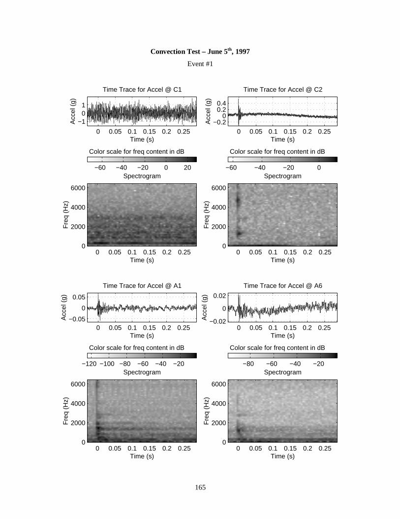
165

Convection Test – June 5th, 1997

Event #1

0 0.05 0.1 0.15 0.2 0.25

−101


Time (s)

Acc

el (

g)

Time (s)

Fre

q (H

z)

Spectrogram


0 0.05 0.1 0.15 0.2 0.250

2000

4000

6000

−60 −40 −20 0 20

0 0.05 0.1 0.15 0.2 0.25−0.2

00.20.4


Time (s)

Acc

el (

g)

Time (s)

Fre

q (H

z)

Spectrogram


0 0.05 0.1 0.15 0.2 0.250

2000

4000

6000

−60 −40 −20 0

0 0.05 0.1 0.15 0.2 0.25−0.05

0

0.05


Time (s)

Acc

el (

g)

Time (s)

Fre

q (H

z)

Spectrogram


0 0.05 0.1 0.15 0.2 0.250

2000

4000

6000

−120 −100 −80 −60 −40 −20

0 0.05 0.1 0.15 0.2 0.25−0.02

0

0.02


Time (s)

Acc

el (

g)

Time (s)

Fre

q (H

z)

Spectrogram


0 0.05 0.1 0.15 0.2 0.250

2000

4000

6000

−80 −60 −40 −20

166

Convection Test – June 23rd, 1997

0 50 100 150 200 250−30

−20

−10

0

10

20

30

40


Time (min)

Tem

pera

ture

(de

g C

)

1 2

T5T7T8T9

A2

C1

C2

T5T7

T8

T9 (ambient)

A4

167


Event #1

0 0.02 0.04 0.06

−1

0

1


Time (s)

Acc

el (

g)

Time (s)

Fre

q (H

z)

Spectrogram


0 0.02 0.04 0.060

1

2

x 104

−80 −60 −40 −20 0 20

0 0.02 0.04 0.06−0.6−0.4−0.2

00.20.4


Time (s)

Acc

el (

g)

Time (s)

Fre

q (H

z)

Spectrogram


0 0.02 0.04 0.060

1

2

x 104

−80 −60 −40 −20 0 20

0 0.02 0.04 0.06−0.1

−0.050

0.05


Time (s)

Acc

el (

g)

Time (s)

Fre

q (H

z)

Spectrogram


0 0.02 0.04 0.060

1

2

x 104

−100 −50 0

0 0.02 0.04 0.06

−0.05

0

0.05Time Trace for Accel @ A4

Time (s)

Acc

el (

g)

Time (s)

Fre

q (H

z)

Spectrogram


0 0.02 0.04 0.060

1

2

x 104

−100 −80 −60 −40 −20 0

168


Event #2

0 0.02 0.04 0.06−1

0


Time (s)

Acc

el (

g)

Time (s)

Fre

q (H

z)

Spectrogram


0 0.02 0.04 0.060

1

2

x 104

−60 −40 −20 0 20

0 0.02 0.04 0.06−1

0


Time (s)

Acc

el (

g)

Time (s)

Fre

q (H

z)

Spectrogram


0 0.02 0.04 0.060

1

2

x 104

−80 −60 −40 −20 0

0 0.02 0.04 0.06−0.04−0.02

00.020.040.06


Time (s)

Acc

el (

g)

Time (s)

Fre

q (H

z)

Spectrogram


0 0.02 0.04 0.060

1

2

x 104

−100 −80 −60 −40 −20 0

Accelerometer A2

not connected to

data acquisition unit

169

Convection Test – August 28th, 1997

0 20 40 60 80 100 120 140 160−30

−20

−10

0

10

20

30

40

50Temperature Profiles for Convection Test (Aug 28, 1997)

Time (min)

Tem

pera

ture

(de

g C

)

1

T1T2

C1

C2C3

C4

A1

A6

C5

C6

T1

T2 (ambient)

Test Procedure Notes: 1st data acquisition unit did not trigger on events (channels C1, C2, C3 &

C4 not available)

170

Convection Test – August 28th, 1997

Event #1

0 0.02 0.04 0.06−0.1

−0.050

0.05


Time (s)

Acc

el (

g)

Time (s)

Fre

q (H

z)

Spectrogram


0 0.02 0.04 0.060

1

2

x 104

−60 −40 −20 0

0 0.02 0.04 0.06

−0.05

0

0.05


Time (s)

Acc

el (

g)

Time (s)

Fre

q (H

z)

Spectrogram


0 0.02 0.04 0.060

1

2

x 104

−60 −40 −20 0

0 0.02 0.04 0.06−0.2

0

0.2


Time (s)

Acc

el (

g)

Time (s)

Fre

q (H

z)

Spectrogram


0 0.02 0.04 0.060

1

2

x 104

−80 −60 −40 −20 0

0 0.02 0.04 0.06−0.02−0.01

00.01


Time (s)

Acc

el (

g)

Time (s)

Fre

q (H

z)

Spectrogram


0 0.02 0.04 0.060

1

2

x 104

−80 −60 −40 −20 0

171

Convection Test – September 2nd, 1997

0 50 100 150 200−30

−20

−10

0

10

20

30

40

50Temperature Profiles for Convection Test (Sept 2, 1997)

Time (min)

Tem

pera

ture

(de

g C

)

1 2

T1T2

C1

C2C3

C4

A1

A6

C5

C6

T1

T2 (ambient)

172


Event #1

0 0.02 0.04 0.06−1

−0.50

0.5


Time (s)

Acc

el (

g)

Time (s)

Fre

q (H

z)

Spectrogram


0 0.02 0.04 0.060

1

2

x 104

−60 −40 −20 0 20

0 0.02 0.04 0.06−0.2−0.1

00.1


Time (s)

Acc

el (

g)

Time (s)

Fre

q (H

z)

Spectrogram


0 0.02 0.04 0.060

1

2

x 104

−60 −40 −20 0

0 0.02 0.04 0.06−1

−0.5

0


Time (s)

Acc

el (

g)

Time (s)

Fre

q (H

z)

Spectrogram


0 0.02 0.04 0.060

1

2

x 104

−80 −60 −40 −20 0 20

0 0.02 0.04 0.06−0.04−0.02

00.020.04


Time (s)

Acc

el (

g)

Time (s)

Fre

q (H

z)

Spectrogram


0 0.02 0.04 0.060

1

2

x 104

−80 −60 −40 −20 0

173


Event #1 (continued)

0 0.02 0.04 0.06

−0.20

0.2


Time (s)

Acc

el (

g)

Time (s)

Fre

q (H

z)

Spectrogram


0 0.02 0.04 0.060

1

2

x 104

−80 −60 −40 −20 0 20

0 0.02 0.04 0.06

−0.1−0.05

0


Time (s)

Acc

el (

g)

Time (s)

Fre

q (H

z)

Spectrogram


0 0.02 0.04 0.060

1

2

x 104

−60 −40 −20 0

0 0.02 0.04 0.06

−0.050

0.05


Time (s)

Acc

el (

g)

Time (s)

Fre

q (H

z)

Spectrogram


0 0.02 0.04 0.060

1

2

x 104

−100 −80 −60 −40 −20 0

0 0.02 0.04 0.06−0.1

00.1


Time (s)

Acc

el (

g)

Time (s)

Fre

q (H

z)

Spectrogram


0 0.02 0.04 0.060

1

2

x 104

−100 −80 −60 −40 −20 0

174


Event #2

0 0.02 0.04 0.06

−0.50

0.5


Time (s)

Acc

el (

g)

Time (s)

Fre

q (H

z)

Spectrogram


0 0.02 0.04 0.060

1

2

x 104

−80 −60 −40 −20 0 20

0 0.02 0.04 0.06

−0.2

0


Time (s)

Acc

el (

g)

Time (s)

Fre

q (H

z)

Spectrogram


0 0.02 0.04 0.060

1

2

x 104

−80 −60 −40 −20 0

0 0.02 0.04 0.06

−1−0.5

00.5


Time (s)

Acc

el (

g)

Time (s)

Fre

q (H

z)

Spectrogram


0 0.02 0.04 0.060

1

2

x 104

−60 −40 −20 0 20

0 0.02 0.04 0.06−0.05

0

0.05


Time (s)

Acc

el (

g)

Time (s)

Fre

q (H

z)

Spectrogram


0 0.02 0.04 0.060

1

2

x 104

−100 −80 −60 −40 −20 0

175



0 0.02 0.04 0.06

−0.5

0

0.5


Time (s)

Acc

el (

g)

Time (s)

Fre

q (H

z)

Spectrogram


0 0.02 0.04 0.060

1

2

x 104

−80 −60 −40 −20 0 20

0 0.02 0.04 0.06−0.04−0.02

00.020.040.060.08


Time (s)

Acc

el (

g)

Time (s)

Fre

q (H

z)

Spectrogram


0 0.02 0.04 0.060

1

2

x 104

−80 −60 −40 −20 0

0 0.02 0.04 0.06

−0.050

0.05


Time (s)

Acc

el (

g)

Time (s)

Fre

q (H

z)

Spectrogram


0 0.02 0.04 0.060

1

2

x 104

−80 −60 −40 −20 0

0 0.02 0.04 0.06

−0.10

0.10.2


Time (s)

Acc

el (

g)

Time (s)

Fre

q (H

z)

Spectrogram


0 0.02 0.04 0.060

1

2

x 104

−100 −80 −60 −40 −20 0

176

Radiation Test – September 29th, 1997

0 20 40 60 80 100 120−200

−150

−100

−50

0


Time (min)

Tem

pera

ture

(de

g C

)

1

T2T3T6T7T8

C1

C2C3

C4

T8 (top of shroud)

T2

T3

T1


T4

T5

T6

177

Radiation Test – September 29th, 1997

Event #1

0 0.02 0.04 0.06−0.2−0.1

00.1


Time (s)

Acc

el (

g)

Time (s)

Fre

q (H

z)

Spectrogram


0 0.02 0.04 0.060

1

2

x 104

−80 −60 −40 −20 0

0 0.02 0.04 0.06

−0.2

−0.1


Time (s)

Acc

el (

g)

Time (s)

Fre

q (H

z)

Spectrogram


0 0.02 0.04 0.060

1

2

x 104

−40 −20 0 20

0 0.02 0.04 0.06

−0.3−0.2−0.1

00.1


Time (s)

Acc

el (

g)

Time (s)

Fre

q (H

z)

Spectrogram


0 0.02 0.04 0.060

1

2

x 104

−80 −60 −40 −20 0

0 0.02 0.04 0.06−1

−0.50

0.5


Time (s)

Acc

el (

g)

Time (s)

Fre

q (H

z)

Spectrogram


0 0.02 0.04 0.060

1

2

x 104

−80 −60 −40 −20 0

178

Radiation Test – October 3rd, 1997

0 20 40 60 80 100 120 140−50

−40

−30

−20

−10

0

10

20

30

40

50Temperature Profiles for Radiation Test (Oct 03, 1997)

Time (min)

Tem

pera

ture

(de

g C

)

1 2

T2T3T6T7T8

C1

C2C3

C4

T2T3

T1

T4

T5

T6

T8 (on plate)

T7 (on plate)

C6

C5

S1

Test Procedure Notes: controlled radiation test using plate instead of shroud; 100kHz BW

setting on 2nd data acquisition unit; DC coupling on strain gauge S1; 1st data acquisition unit did

not trigger on events (channels C1, C2, C3 & C4 not available)

179


Event #1

0 5 10

x 10−3

−0.4−0.2

00.20.4


Time (s)A

ccel

(g)

Time (s)

Fre

q (H

z)

Spectrogram


0 5 10

x 10−3

0

5

10

x 104−40 −20 0 20

0 5 10

x 10−3

−2

0

2


Time (s)

Acc

el (

g)

Time (s)

Fre

q (H

z)

Spectrogram


0 5 10

x 10−3

0

5

10

x 104

−60 −40 −20 0 20

0 5 10

x 10−3

−5

0Time Trace for SG Output @ S1

Time (s)

SG

Out

put (

V)

Time (s)

Fre

q (H

z)

Spectrogram


0 5 10

x 10−3

0

5

10

x 104

−50 0 50

180


Event #2

0 5 10

x 10−3

−0.4−0.2

00.20.4


Time (s)A

ccel

(g)

Time (s)

Fre

q (H

z)

Spectrogram


0 5 10

x 10−3

0

5

10

x 104

−40 −20 0 20

0 5 10

x 10−3

−20

0


Time (s)

Acc

el (

g)

Time (s)

Fre

q (H

z)

Spectrogram


0 5 10

x 10−3

0

5

10

x 104

−60 −40 −20 0 20 40

0 5 10

x 10−3

−5

0Time Trace for SG Output @ S1

Time (s)

SG

Out

put (

V)

Time (s)

Fre

q (H

z)

Spectrogram


0 5 10

x 10−3

0

5

10

x 104

−60 −40 −20 0 20 40

181

Radiation Test – October 8th, 1997

0 20 40 60 80 100 120 140 160−50

−40

−30

−20

−10

0

10

20

30

40

50Temperature Profiles for Radiation Test (Oct 08, 1997)

Time (min)

Tem

pera

ture

(de

g C

)

1 2

T2T3T6T7T8

C1

C2C3

C4

T2T3

T1

T4

T5

T6

T8 (on plate)

T7 (on plate)

C6

C5

S1

Test Procedure Notes: controlled radiation test using plate instead of shroud; 100kHz BW

setting on 2nd data acquisition unit; AC coupling on strain gauge S1; 1st data acquisition unit did

not trigger on events (channels C1, C2, C3 & C4 not available)

182


Event #1

0 5 10

x 10−3

−1

0


Time (s)A

ccel

(g)

Time (s)

Fre

q (H

z)

Spectrogram


0 5 10

x 10−3

0

5

10

x 104

−60 −40 −20 0 20

0 5 10

x 10−3

−202


Time (s)

Acc

el (

g)

Time (s)

Fre

q (H

z)

Spectrogram


0 5 10

x 10−3

0

5

10

x 104

−40 −20 0 20

0 5 10

x 10−3

0

1

2

x 10−3 Time Trace for SG @ S1

Time (s)

SG

(V

)

Time (s)

Fre

q (H

z)

Spectrogram


0 5 10

x 10−3

0

5

10

x 104

−100 −80 −60 −40 −20

183


Event #2

0 5 10

x 10−3

−5

0

5


Time (s)A

ccel

(g)

Time (s)

Fre

q (H

z)

Spectrogram


0 5 10

x 10−3

0

5

10

x 104

−60 −40 −20 0 20 40

0 5 10

x 10−3

−1.5−1

−0.50

0.5


Time (s)

Acc

el (

g)

Time (s)

Fre

q (H

z)

Spectrogram


0 5 10

x 10−3

0

5

10

x 104

−60 −40 −20 0 20

0 5 10

x 10−3

0

1

2

x 10−3 Time Trace for SG @ S1

Time (s)

SG

(V

)

Time (s)

Fre

q (H

z)

Spectrogram


0 5 10

x 10−3

0

5

10

x 104

−120 −100 −80 −60 −40 −20

184

Radiation Test – November 25th, 1997

0 50 100 150−200

−150

−100

−50

0

50

100Temperature Profiles for Radiation Test (Nov 25, 1997)

Time (min)

Tem

pera

ture

(de

g C

)

1

T2T3T6T7T9

C4

T3

T1

T5

T4 S1C5

T8 (back wall)

T7 (top of shroud)

C3T2

C2 C6

C1

T6


Test Procedure Notes: 100 kHz BW setting on 1st data acquisition unit (channels C2, C3 &C6)

185


Event #1

0 5 10

x 10−3

−2

0

2


Time (s)A

ccel

(g)

Time (s)

Fre

q (H

z)

Spectrogram


0 5 10

x 10−3

0

5

10

x 104

−40 −20 0 20 40

0 5 10

x 10−3

−0.2

0

0.2


Time (s)

Acc

el (

g)

Time (s)

Fre

q (H

z)

Spectrogram


0 5 10

x 10−3

0

5

10

x 104

−40 −20 0 20

0 5 10

x 10−3

−0.10

0.10.2


Time (s)

Acc

el (

g)

Time (s)

Fre

q (H

z)

Spectrogram


0 5 10

x 10−3

0

5

10

x 104

−60 −40 −20 0 20

186



0 0.02 0.04 0.06

−101


Time (s)

Acc

el (

g)

Time (s)

Fre

q (H

z)

Spectrogram


0 0.02 0.04 0.060

1

2

x 104

−60 −40 −20 0 20

0 0.02 0.04 0.06

−0.5

0

0.5


Time (s)

Acc

el (

g)

Time (s)

Fre

q (H

z)

Spectrogram


0 0.02 0.04 0.060

1

2

x 104

−60 −40 −20 0 20

0 0.02 0.04 0.06

−0.2

0


Time (s)

Acc

el (

g)

Time (s)

Fre

q (H

z)

Spectrogram


0 0.02 0.04 0.060

1

2

x 104

−60 −40 −20 0 20

0 0.02 0.04 0.06−0.01

0

0.01Time Trace for SG Output @ S1

Time (s)

SG

Out

put (

V)

Time (s)

Fre

q (H

z)

Spectrogram


0 0.02 0.04 0.060

1

2

x 104

−80 −60 −40

Microdynamics and Thermal Snap Response of...

Documents

Transcript of Microdynamics and Thermal Snap Response of...