Micro-plasticity and intermittent dislocation activity in a simplified micro-structural model

This article has been downloaded from IOPscience. Please scroll down to see the full text article.

2013 Modelling Simul. Mater. Sci. Eng. 21 035007

(http://iopscience.iop.org/0965-0393/21/3/035007)

Download details:

IP Address: 192.33.118.220

The article was downloaded on 02/03/2013 at 09:25

Please note that terms and conditions apply.

View the table of contents for this issue, or go to the journal homepage for more

Home Search Collections Journals About Contact us My IOPscience

IOP PUBLISHING MODELLING AND SIMULATION IN MATERIALS SCIENCE AND ENGINEERING

Modelling Simul. Mater. Sci. Eng. 21 (2013) 035007 (22pp) doi:10.1088/0965-0393/21/3/035007

Micro-plasticity and intermittent dislocation activityin a simplified micro-structural model

P M Derlet1 and R Maaß2

1 Condensed Matter Theory Group, Paul Scherrer Institut, CH-5232 Villigen PSI, Switzerland2 California Institute of Technology, Division of Engineering and Applied Sciences, 1200 ECalifornia Blvd, Pasadena, CA 91125-810 0, USA

E-mail: Peter.Derlet@psi.ch and maass@caltech.edu

Received 7 August 2012, in final form 20 December 2012Published 1 March 2013Online at stacks.iop.org/MSMSE/21/035007

AbstractHere we present a model to study the micro-plastic regime of a stress–straincurve. In this model an explicit dislocation population represents the mobiledislocation content and an internal shear-stress field represents a mean-fielddescription of the immobile dislocation content. The mobile dislocations areconstrained to a simple dipolar mat geometry and modelled via a dislocationdynamics (DD) algorithm, whilst the shear-stress field is chosen to be asinusoidal function of distance along the mat direction. The sinusoidal function,defined by a periodic length and a shear-stress amplitude, is interpreted torepresent a pre-existing micro-structure. These model parameters, alongwith the mobile dislocation density, are found to admit a diversity of micro-plastic behaviour involving intermittent plasticity in the form of a scale-freeavalanche phenomenon, with an exponent and scaling-collapse for the strain-burst magnitude distribution that is in agreement with mean-field theory andsimilar to that seen in experiment and more complex DD simulations.

(Some figures may appear in colour only in the online journal)

1. Introduction

In 1964, using state-of-the-art torsion experiments, Tinder and co-workers were able to achievea strain resolution of 10−8 for sub-millimeter-sized samples to study the micro-plastic regimeof highly pure poly-crystal Cu samples [1], followed by tests on Zn single crystals someyears later [2]. Their plastic strain versus stress curves contained plateaus of stress which wereattributed to the occurrence of discrete dislocation glide activity over a length scale comparableto the dislocation spacing of an assumed three-dimensional network. Indeed the authors writein [1], ‘The results suggest that an important fraction of the total strain, in the initial stagesof deformation, involved motion of a few favourably situated dislocation segments throughdistances large enough to form new interactions with other elements of the three-dimensional

0965-0393/13/035007+22$33.00 © 2013 IOP Publishing Ltd Printed in the UK & the USA 1

Modelling Simul. Mater. Sci. Eng. 21 (2013) 035007 P M Derlet and R Maaß

network. If this were so, then most elements of the network must have been relatively immobile,making little or no contribution to the strain.’ That most dislocations remain immobile remainsa contemporary viewpoint [3].

Another more recently pursued route is to probe discrete dislocation activity via thestress-strain curve of micrometre-sized focused ion beam (FIB) milled single crystals. Here,advantage is taken of a nano-indentation platform equipped with a flat punch tip to compressmicro-/nano-crystals [4–7]. In addition to the sub-nanometre displacement resolution ofthe system, which notably has a lower strain resolution than the above mentioned torsionexperiments, the sample size is decreased to the micrometre range and below. As a result,the strain associated with the discrete dislocation activity is increased to an easily detectablemagnitude. Whilst this more contemporary work has been primarily motivated by the ‘smaller-is-stronger’ size-effect paradigm [4, 5, 8–10], an extensive analysis of the statistics of thediscrete dislocation activity has revealed power-law behaviour in the distribution of strain-burstmagnitudes giving an exponent of ≈1.6–2.2 [6, 7, 11]. Similar exponents can also be found inbulk samples via detailed analysis of load displacement signals, where structural evolution isalso seen to occur [12, 13]. The very recent work of Dahmen and co-workers [14, 15] suggestthat the variation in literature exponent values could be due to the different stress intervals usedto bin the strain-burst magnitude data, where a total integration over the stress interval fromzero to the yield stress should, within mean-field theory (MFT), give an exponent equal toprecisely two. Such exponents are indicative of crackling [16] or Barkhausen noise, and moregenerally of avalanche phenomena, indicating that dislocation mediated plastic deformationbelongs to a universality class that encompasses many natural phenomenon over a variety ofdifferent length and timescales. Indeed, similar power-law exponents can also be found formetallic glasses [17] in which the underlying plastic deformation is fundamentally different tocrystalline metals.

Another class of experiments revealing the intermittent nature of dislocation dynamics(DD) is the acoustic emission monitoring of ice [18, 19]. Such experiments measure theacoustic energy released by intermittent dislocation activity during constant stress deformation(in the tertiary creep regime). Indeed, via single sensor acoustic emission signals, suchdislocation activity can be well characterized in time revealing power-law behaviour withexponents of 1.6–1.8, which is very similar to that seen via the micro-compression stress-strain curves [6, 7, 11]. Furthermore, via multiple sensor monitoring, time and space clusteringof dislocation avalanches could be observed [19]. It was found that avalanche epi-centreswere correlated in space according to a non-integer power-law exponent indicating scale-freeclustering and at short enough times such clusters were correlated in time, indicating collectiveactivity.

That such scale-invariant dislocation activity occurs is a signature of an underlyingcomplex dislocation based micro-structure. An entity whose properties and evolution underan applied stress play a central role in the more general subjects of material strength andstrain hardening [20]. Due to the complex dynamics and evolution of the dislocation structure,computer simulation based approaches have helped greatly over the past decades to clarifythe underlying dislocation based mechanisms responsible for such structural evolution. Onesuch method is the so-called DD approach. Early work involved two-dimensional arraysof straight edge dislocations interacting via elasticity using single- and multi-slip geometries[21–23]. These works demonstrate that under an external stress, dislocation patterning emergesanalogous to what is seen in static transmission electron microscopy experiments. Other andmore recent works have developed these numerical techniques in terms of efficiency [24],strain boundary conditions and obstacle/composite geometries [25] to study more complexpatterning such as the emergence of granular cell structures and the study of grain boundary

2

Modelling Simul. Mater. Sci. Eng. 21 (2013) 035007 P M Derlet and R Maaß

network evolution [26], strain hardening, and material strength in both bulk and confinedvolume systems [27, 28]. Analogous methodologies and investigations have also been carriedout in three dimensions [29–33].

Intermittent dislocation activity, in the form of dislocation avalanches, has also beenstudied using the DD simulation technique [18, 28, 31]. Such simulations have producedpower-law exponents of the distribution of strain-burst magnitudes similar to that seen inexperiments, indicating some degree of scale-free behaviour, where dislocations are arranged inmeta-stable cell and/or wall structures, with only a minor fraction of the dislocation populationmoving intermittently, thereby creating discrete strain jumps. The so-called self-organizedcriticality (SOC) view of the dislocation network state offers one theoretical platform for theunderstanding of the observed universality [34], in which the material system organizes itselfinto a configuration that is critical, resulting in scale-free behaviour upon transiting to a newrealization of the critical state. Originally developed to describe sand-pile dynamics [35], theapproach is somewhat at odds with the historical viewpoint that dislocation structure evolutionis primarily driven by equilibrium driving forces such as that embodied in low energy structures(LES) theory [36] and in a wide range of strain hardening theories. The finding that theoccurrence of avalanche phenomenon is insensitive to the nature of the forming immobiledislocation network, the slip geometry, the deformation mode, and the details of the DD andspatial dimension is a central hallmark of SOC, which is robust against the details of theunderlying physical model.

This motivates investigating plastic flow with simpler models that explicitly do not takeinto account the fine details of individually interacting sessile and mobile dislocations, naturallyshifting the focus of plastic flow from complex dislocation structural evolution to the interactionof a minute mobile dislocation population with a simplified description of the sessile dislocationpopulation. Such an approach is analogous to the study of dislocations in the presence ofpinning potentials [37, 38] and more generally to coarse grained models of plasticity that studythe depinning transition (see [34] and references therein, and also [14, 15]). Dislocation fieldtheories are also very able to study intermittency; however, unlike DD based methods whichare able to simulate only small plastic strains, these models are able to incorporate dislocationtransport over non-negligible distances and therefore able to simulate significant structuralevolution [12].

In this work, a simple model is therefore proposed in which a dipolar dislocation mat [41]is embedded into an internal static sinusoidal stress field defined by a wavelength and a shear-stress amplitude. The explicit dislocation population is modelled via a standard DD algorithm.It is found that, similar to very complex and detailed 3D-DD simulations, the resulting stress-strain curves evolve in a discrete manner that reflects an underlying intermittent plasticityoriginating from irreversible changes in dislocation configuration, and that the distributionof the corresponding strain-burst magnitudes reveal both extremal value statistics and scale-free avalanche behaviour. Thus, although the complex details of microscopic dislocationmechanisms and structure are omitted, the simple model is still able to capture the fundamentalproperties of intermittent micro-plastic flow.

In the following section, the model is formally introduced and the DD technique described,and in section 3 various loading modes to produce a stress-strain curve are presented. Section 4presents the DD simulations for a wide range of model parameters to investigate their effecton deformation behaviour. The statistical analysis of the stress at which intermittent activityoccurs, as well as the distribution of related strain bursts, are presented in section 5. Finally,section 6 discusses the context for the model, where it is argued that its applicable range isrestricted to the micro-plastic region of the stress-strain curve—a regime where significantstructural evolution and work hardening are, to a large extent, absent [39, 40].

3

Modelling Simul. Mater. Sci. Eng. 21 (2013) 035007 P M Derlet and R Maaß

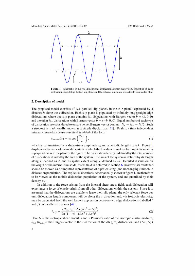
Figure 1. Schematic of the two-dimensional dislocation dipolar mat system consisting of edgedislocations populating the two slip planes and the external sinusoidal stress field visualized in blue.

2. Description of model

The proposed model consists of two parallel slip planes, in the x–z plane, separated by adistance h along the y direction. Each slip plane is populated by infinitely long straight edgedislocations where one slip plane contains N+ dislocations with Burgers vector �b = (b, 0, 0)

and the other N− dislocations with Burgers vector �b = (−b, 0, 0). Equal numbers of each typeof dislocation are considered to ensure no net Burgers vector content: N+ = N− = N/2. Sucha structure is traditionally known as a simple dipolar mat [41]. To this, a time independentinternal sinusoidal shear-stress field is added of the form

τInternal(x) = τ0 cos

(2πx

λ

), (1)

which is parametrized by a shear-stress amplitude τ0 and a periodic length scale λ. Figure 1displays a schematic of the model system in which the line direction of each straight dislocationis perpendicular to the plane of the figure. The dislocation density is defined by the total numberof dislocations divided by the area of the system. The area of the system is defined by its lengthalong x, defined as d , and its spatial extent along y, defined as 2h. Detailed discussion onthe origin of the internal sinusoidal stress field is deferred to section 6; however, its existenceshould be viewed as a simplified representation of a pre-existing (and unchanging) immobiledislocation population. The explicit dislocations, schematically shown in figure 1, are thereforeto be viewed as the mobile dislocation population of the system, and are quantified by theirdensity ρm.

In addition to the force arising from the internal shear-stress field, each dislocation willexperience a force of elastic origin from all other dislocations within the system. Since it isassumed that the dislocations are unable to leave their slip plane, the only relevant force perunit dislocation length component will be along the x direction and, via isotropic elasticity,may be calculated from the well known expression between two edge dislocations (labelled i

and j ) on parallel slip planes [42]

fx,ij = Gbx,ibx,j

2π(1 − ν)

�x(�x2 − �y2)

(�x2 + �y2)2. (2)

Here G is the isotropic shear modulus and ν Possion’s ratio of the isotropic elastic medium,bx,i (bx,j ) is the Burgers vector in the x-direction of the ith (j th) dislocation, and (�x, �y)

4

Modelling Simul. Mater. Sci. Eng. 21 (2013) 035007 P M Derlet and R Maaß

is the two-dimensional vector defining the dislocations’ spatial separation. Presently a modelisotropic Cu system is implemented, in which the shear modulus is taken as G = 42 GPa, thePossion’s ratio as µ = 0.43 and the Burgers vector magnitude as b = 2.55 Å.

For this work, periodic boundary conditions along d, the dipolar mat direction and openboundary conditions along h, are assumed. Due to the long range nature of equation (2), thecorrect treatment of periodicity involves the summation of all dislocation image contributions tothe force per unit dislocation length on a given dislocation. For the considered one-dimensionalperiodicity, an exact solution to such a summation is tractable, and is given by

fx,ij = −Gbx,ibx,j

2(1 − ν)sin

(2π�x

d

) [d

(cos

(2π�x

d

) − cosh(

2π�y

d

))+ 2π�y sin

(2π�y

d

)]

d2(

cos(

2π�xd

) − cosh(

2π�y

d

))2 .

(3)

A simple derivation of this equation is detailed in the appendix.The temporal evolution of a particular dislocation configuration is characterized by the

choice of an empirical mobility law. Due to the actual discreteness of the lattice at the atomicscale, a dislocation segment must overcome an energy barrier associated with the local shearingof atoms in order to move an atomic distance. This so-called Peierls energy barrier and theassociated Peierls stress [43], the stress at which the dislocation can begin to move (defined ata given temperature), results in the dislocation moving quasi-statically from atomic lattice siteto atomic lattice site. At the meso-scopic scale this results in over-damped motion where thedislocation’s velocity is proportional to the force acting on the dislocation—the present mobilitylaw. The material specific proportionality constant is referred to as a damping parameter andis dependent on dislocation type, geometry and temperature.

The equation of motion along the x direction for the ith dislocation is then given by

δxi

δt= Fx,i

B, (4)

where B is the damping coefficient, which for Cu is 5 × 10−5 Pa s [23, 44]. In equation (4),Fx,i , is the total force per unit dislocation length acting on the dislocation,

Fx,i = [τInternal(xi) − τExternal] bx,i +∑j �=i

fx,ij . (5)

Here τExternal is an externally applied homogeneous shear-stress field and τInternal is the staticsinusoidal shear-stress field defined in equation (1).

The numerical solution of equation (4) constitutes the DD algorithm presently used inwhich an appropriate finite time-step, δt , is used to integrate the equations of motion. Thecorresponding shear-strain response δε within this δt is calculated via

δε = 1

2dh

N∑i

bx,iδxi . (6)

It is again emphasized that over the timescale of δt all atomic scale aspects are averaged overand inertial effects are ignored. Since the edge dislocations are infinitely long and straightsuch dynamics falls into the class of two-dimensional DD modelling.

The dislocation density is given by ρm = N/2dh. For this work, the periodic length d ischosen to define the distance h between the two populated slip systems via 2d/N . This sets themean distance between dislocations along the x- and y-direction to be the same, and definesthe dislocation density as (N/2d)2. Thus, h = 1/

√ρm, and choosing a value of the dislocation

density will fix the scale of interaction between the two parallel slip planes of the dipolar mat

5

Modelling Simul. Mater. Sci. Eng. 21 (2013) 035007 P M Derlet and R Maaß

05e-06

1e-051.5e-05

2e-052.5e-05

plastic shear strain

0

10

20

30

40

shea

r st

ress

(M

Pa)

0.00078 0.000795 0.00081 0.000825

total shear strain

32

32.5

33

33.5

34

(a) (b)

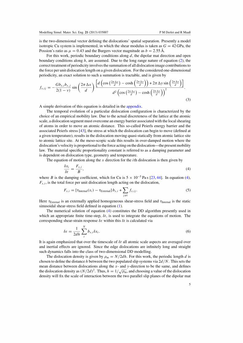
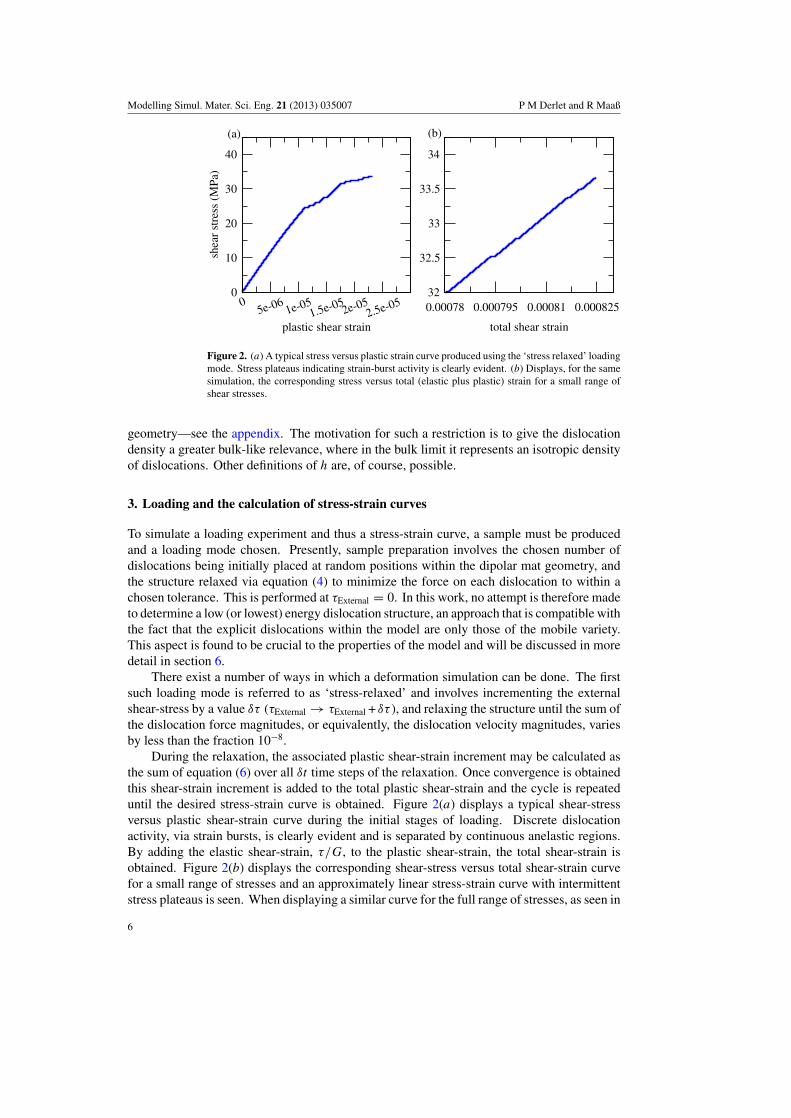
Figure 2. (a) A typical stress versus plastic strain curve produced using the ‘stress relaxed’ loadingmode. Stress plateaus indicating strain-burst activity is clearly evident. (b) Displays, for the samesimulation, the corresponding stress versus total (elastic plus plastic) strain for a small range ofshear stresses.

geometry—see the appendix. The motivation for such a restriction is to give the dislocationdensity a greater bulk-like relevance, where in the bulk limit it represents an isotropic densityof dislocations. Other definitions of h are, of course, possible.

3. Loading and the calculation of stress-strain curves

To simulate a loading experiment and thus a stress-strain curve, a sample must be producedand a loading mode chosen. Presently, sample preparation involves the chosen number ofdislocations being initially placed at random positions within the dipolar mat geometry, andthe structure relaxed via equation (4) to minimize the force on each dislocation to within achosen tolerance. This is performed at τExternal = 0. In this work, no attempt is therefore madeto determine a low (or lowest) energy dislocation structure, an approach that is compatible withthe fact that the explicit dislocations within the model are only those of the mobile variety.This aspect is found to be crucial to the properties of the model and will be discussed in moredetail in section 6.

There exist a number of ways in which a deformation simulation can be done. The firstsuch loading mode is referred to as ‘stress-relaxed’ and involves incrementing the externalshear-stress by a value δτ (τExternal → τExternal + δτ ), and relaxing the structure until the sum ofthe dislocation force magnitudes, or equivalently, the dislocation velocity magnitudes, variesby less than the fraction 10−8.

During the relaxation, the associated plastic shear-strain increment may be calculated asthe sum of equation (6) over all δt time steps of the relaxation. Once convergence is obtainedthis shear-strain increment is added to the total plastic shear-strain and the cycle is repeateduntil the desired stress-strain curve is obtained. Figure 2(a) displays a typical shear-stressversus plastic shear-strain curve during the initial stages of loading. Discrete dislocationactivity, via strain bursts, is clearly evident and is separated by continuous anelastic regions.By adding the elastic shear-strain, τ/G, to the plastic shear-strain, the total shear-strain isobtained. Figure 2(b) displays the corresponding shear-stress versus total shear-strain curvefor a small range of stresses and an approximately linear stress-strain curve with intermittentstress plateaus is seen. When displaying a similar curve for the full range of stresses, as seen in

6

Modelling Simul. Mater. Sci. Eng. 21 (2013) 035007 P M Derlet and R Maaß

figure 2(a), only a straight line is resolvable, indicating that such strain bursts are well withinthe micro-plastic regime of deformation. At larger stresses a plastic flow regime is enteredwhich will be investigated in more detail in subsequent sections.

Experimentally, two distinct deformation modes can be used: displacement controlledand load controlled. Here we consider an inherently force controlled testing device. In sucha case, displacement controlled testing is done by adjusting the applied load via a feed-backloop such that the displacement rate is held at a fixed value throughout the loading, whereasfor load controlled experiments, the applied load simply increases at a chosen rate. For thepresent model, these deformation modes correspond to a constant shear-strain rate and constantshear-stress rate loading condition. To obtain a stress-strain curve with a constant shear-stressrate, a numerical value for the applied stress rate, τExternal, is chosen. This then defines a stressincrement δτ = τExternalδt , where δt is the time-step used to evolve the dislocation networkaccording to equation (4). Thus at every simulation iteration, the stress is increased by δτ

and the configuration evolves in time by an amount δt . To implement a constant shear-strainrate loading mode, ε, a numerical value is chosen and the appropriate δτ stress increment,to achieve such a strain rate, is performed every simulation step. The actual value of δτ isdetermined by assuming that the total strain rate decomposes additively into an elastic andplastic component:

ε = εelastic + εplastic = τExternal

G+ εplastic, (7)

giving

τExternal = G(ε − εplastic

)(8)

or

δτ = G(ε − εplastic

)δt, (9)

where εplasticδt is the strain increment per simulation iteration, calculated via equation (6). Thusthe stress increment δτ is determined by the correction needed to achieve the required constantstrain rate for the next simulation iteration. In the above, due to the simplified geometry of themodel (figure 1), a pure shear modulus, G, rather than a Young’s modulus is used.

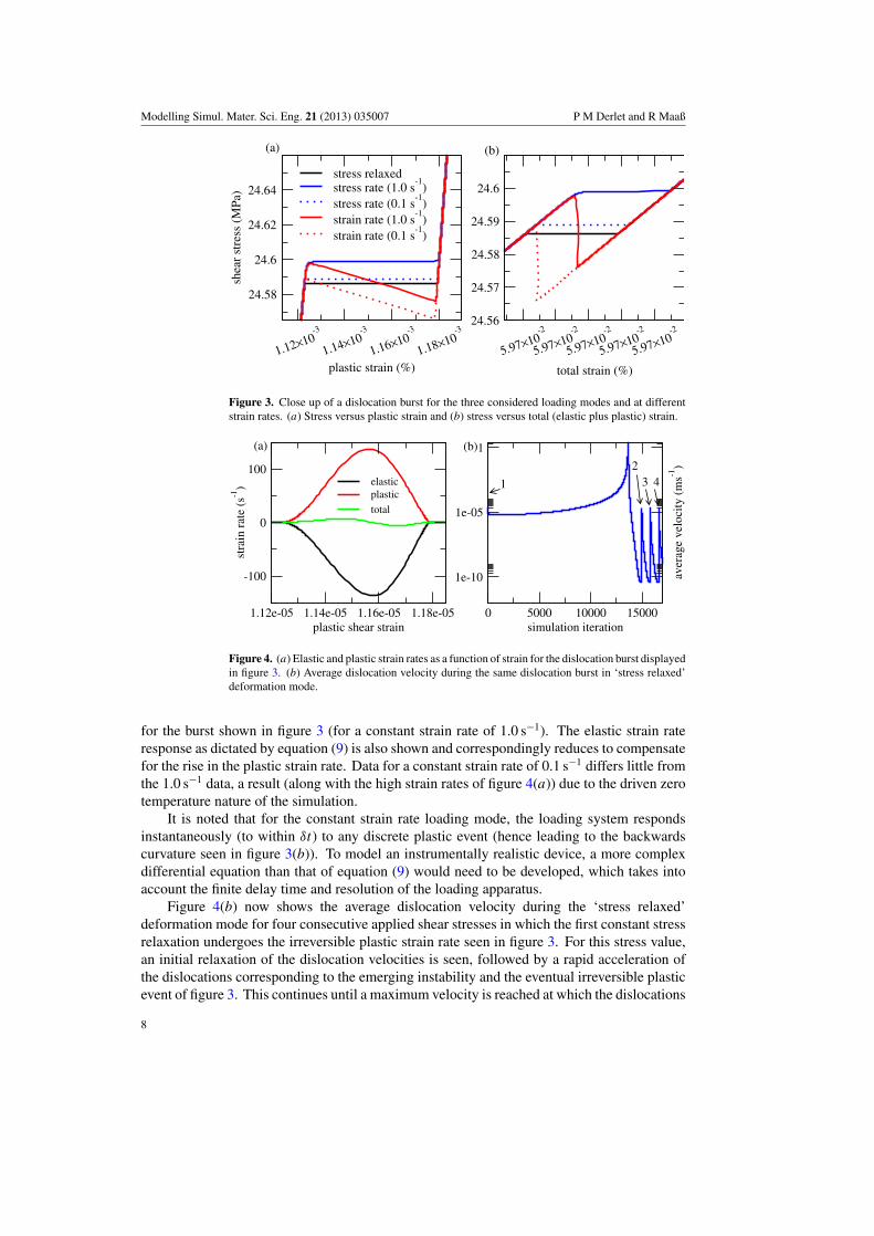
To investigate how such loading modes affect the discrete dislocation activity seen infigure 2, the appropriate stress rate and strain rate must be chosen. This is done by firstchoosing ε, from which τExternal is obtained via ε/G to ensure that in the elastic/anelasticregime both deformation modes have the same total strain rate. Figure 3 displays a singlestrain burst in all three considered loading modes. For the constant strain rate and stress ratemodes two strain rates are considered: 0.1 and 1.0 s−1. For the ‘stress-relaxed’ loading modea sharp plateau is evident in figure 3(a) with an identically zero gradient. In this region, theconstant stress rate mode also exhibits a plateau but with a (non-zero) positive gradient since,during the evolution of the strain burst, the stress is rising at the chosen rate. Also, the stress atwhich the strain burst initiates is somewhat higher (and increasing with increasing strain rate)than that in the stress relaxed mode indicating a strain-rate effect. In this regard, the ‘stress-relaxed’ deformation mode can be considered as the zero stress-rate limit of the constant stressrate loading mode in which the dislocation configuration always has time to relax before thenext stress increment. For the constant strain-rate loading mode, the onset of the strain burstoccurs at similar stresses to that of the constant stress rate; however, as the strain-burst evolves,the stress decreases to maintain the chosen strain rate. Figure 3(b) displays the same strainburst with the stress now as a function of the total strain. The greatest effect is seen in theconstant strain-rate mode where due to the drop in stress during the strain burst, there is a rapiddrop in elastic strain. Figure 4(a) displays the plastic strain rate as a function of plastic strain

7

Modelling Simul. Mater. Sci. Eng. 21 (2013) 035007 P M Derlet and R Maaß

1.12×10-3

1.14×10-3

1.16×10-3

1.18×10-3

plastic strain (%)

24.58

24.6

24.62

24.64

shea

r st

ress

(M

Pa)

stress relaxedstress rate (1.0 s

-1)

stress rate (0.1 s-1

)strain rate (1.0 s

-1)

strain rate (0.1 s-1

)

5.97×10-2

5.97×10-2

5.97×10-2

5.97×10-2

5.97×10-2

total strain (%)

24.56

24.57

24.58

24.59

24.6

(a) (b)

Figure 3. Close up of a dislocation burst for the three considered loading modes and at differentstrain rates. (a) Stress versus plastic strain and (b) stress versus total (elastic plus plastic) strain.

1.12e-05 1.14e-05 1.16e-05 1.18e-05plastic shear strain

-100

0

100

stra

in r

ate

(s-1

) elasticplastic

total

0 5000 10000 15000simulation iteration

1e-10

1e-05

1

aver

age

velo

city

(m

s-1)

(a) (b)

1 42

3

Figure 4. (a) Elastic and plastic strain rates as a function of strain for the dislocation burst displayedin figure 3. (b) Average dislocation velocity during the same dislocation burst in ‘stress relaxed’deformation mode.

for the burst shown in figure 3 (for a constant strain rate of 1.0 s−1). The elastic strain rateresponse as dictated by equation (9) is also shown and correspondingly reduces to compensatefor the rise in the plastic strain rate. Data for a constant strain rate of 0.1 s−1 differs little fromthe 1.0 s−1 data, a result (along with the high strain rates of figure 4(a)) due to the driven zerotemperature nature of the simulation.

It is noted that for the constant strain rate loading mode, the loading system respondsinstantaneously (to within δt) to any discrete plastic event (hence leading to the backwardscurvature seen in figure 3(b)). To model an instrumentally realistic device, a more complexdifferential equation than that of equation (9) would need to be developed, which takes intoaccount the finite delay time and resolution of the loading apparatus.

Figure 4(b) now shows the average dislocation velocity during the ‘stress relaxed’deformation mode for four consecutive applied shear stresses in which the first constant stressrelaxation undergoes the irreversible plastic strain rate seen in figure 3. For this stress value,an initial relaxation of the dislocation velocities is seen, followed by a rapid acceleration ofthe dislocations corresponding to the emerging instability and the eventual irreversible plasticevent of figure 3. This continues until a maximum velocity is reached at which the dislocations

8

Modelling Simul. Mater. Sci. Eng. 21 (2013) 035007 P M Derlet and R Maaß

0 5e-06 1e-05 1.5e-05 2e-05plastic shear strain

0.1

1

10

100

shea

r st

ress

(M

Pa)

τ0=100 MPa

τ0=10 MPa

τ0=1 MPa

0 0.001 0.002 0.003total shear strain

0

20

40

60

80

100

(b)(a)

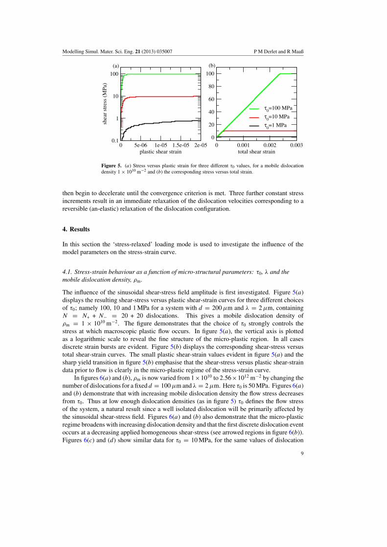
Figure 5. (a) Stress versus plastic strain for three different τ0 values, for a mobile dislocationdensity 1 × 1010 m−2 and (b) the corresponding stress versus total strain.

then begin to decelerate until the convergence criterion is met. Three further constant stressincrements result in an immediate relaxation of the dislocation velocities corresponding to areversible (an-elastic) relaxation of the dislocation configuration.

4. Results

In this section the ‘stress-relaxed’ loading mode is used to investigate the influence of themodel parameters on the stress-strain curve.

4.1. Stress-strain behaviour as a function of micro-structural parameters: τ0, λ and themobile dislocation density, ρm.

The influence of the sinusoidal shear-stress field amplitude is first investigated. Figure 5(a)displays the resulting shear-stress versus plastic shear-strain curves for three different choicesof τ0; namely 100, 10 and 1 MPa for a system with d = 200 µm and λ = 2 µm, containingN = N+ + N− = 20 + 20 dislocations. This gives a mobile dislocation density ofρm = 1 × 1010 m−2. The figure demonstrates that the choice of τ0 strongly controls thestress at which macroscopic plastic flow occurs. In figure 5(a), the vertical axis is plottedas a logarithmic scale to reveal the fine structure of the micro-plastic region. In all casesdiscrete strain bursts are evident. Figure 5(b) displays the corresponding shear-stress versustotal shear-strain curves. The small plastic shear-strain values evident in figure 5(a) and thesharp yield transition in figure 5(b) emphasise that the shear-stress versus plastic shear-straindata prior to flow is clearly in the micro-plastic regime of the stress-strain curve.

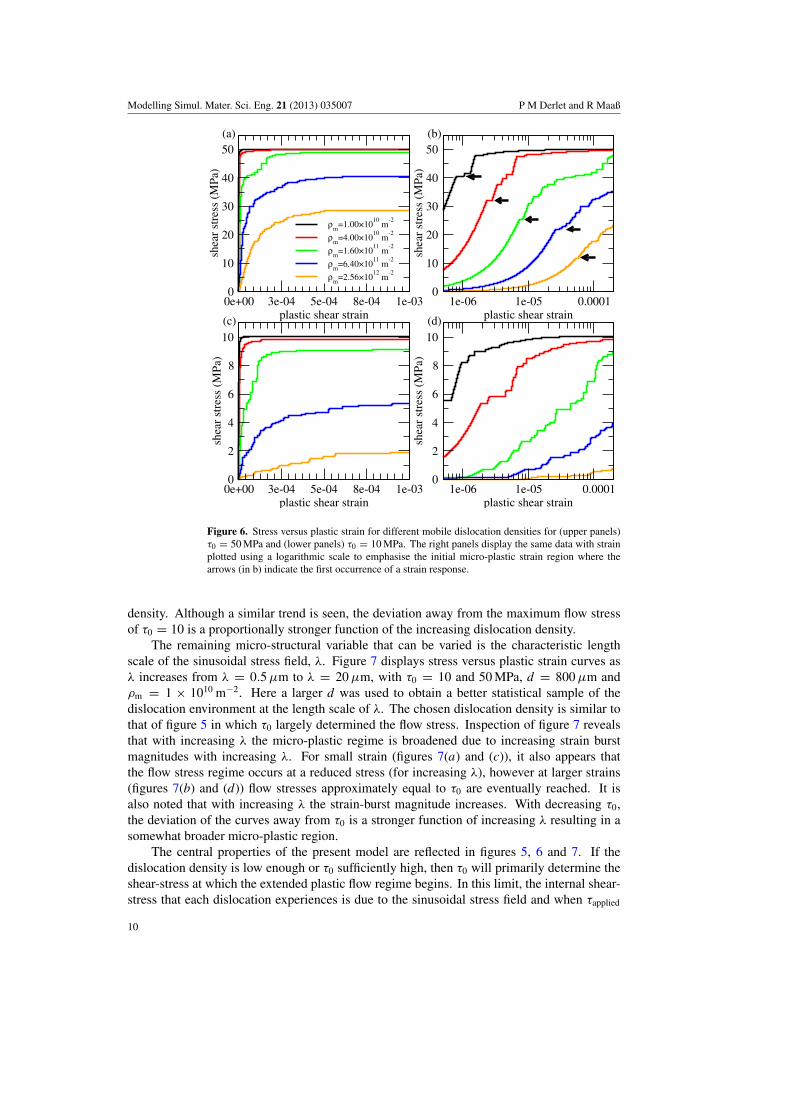
In figures 6(a) and (b), ρm is now varied from 1×1010 to 2.56×1012 m−2 by changing thenumber of dislocations for a fixed d = 100 µm and λ = 2 µm. Here τ0 is 50 MPa. Figures 6(a)and (b) demonstrate that with increasing mobile dislocation density the flow stress decreasesfrom τ0. Thus at low enough dislocation densities (as in figure 5) τ0 defines the flow stressof the system, a natural result since a well isolated dislocation will be primarily affected bythe sinusoidal shear-stress field. Figures 6(a) and (b) also demonstrate that the micro-plasticregime broadens with increasing dislocation density and that the first discrete dislocation eventoccurs at a decreasing applied homogeneous shear-stress (see arrowed regions in figure 6(b)).Figures 6(c) and (d) show similar data for τ0 = 10 MPa, for the same values of dislocation

9

Modelling Simul. Mater. Sci. Eng. 21 (2013) 035007 P M Derlet and R Maaß

0e+00 3e-04 5e-04 8e-04 1e-03plastic shear strain

0

10

20

30

40

50

shea

r st

ress

(M

Pa)

ρm

=1.00×1010

m-2

ρm

=4.00×1010

m-2

ρm

=1.60×1011

m-2

ρm

=6.40×1011

m-2

ρm

=2.56×1012

m-2

1e-06 1e-05 0.0001plastic shear strain

0

10

20

30

40

50

shea

r st

ress

(M

Pa)

0e+00 3e-04 5e-04 8e-04 1e-03plastic shear strain

0

2

4

6

8

10

shea

r st

ress

(M

Pa)

1e-06 1e-05 0.0001plastic shear strain

0

2

4

6

8

10

shea

r st

ress

(M

Pa)

(a) (b)

(d)(c)

Figure 6. Stress versus plastic strain for different mobile dislocation densities for (upper panels)τ0 = 50 MPa and (lower panels) τ0 = 10 MPa. The right panels display the same data with strainplotted using a logarithmic scale to emphasise the initial micro-plastic strain region where thearrows (in b) indicate the first occurrence of a strain response.

density. Although a similar trend is seen, the deviation away from the maximum flow stressof τ0 = 10 is a proportionally stronger function of the increasing dislocation density.

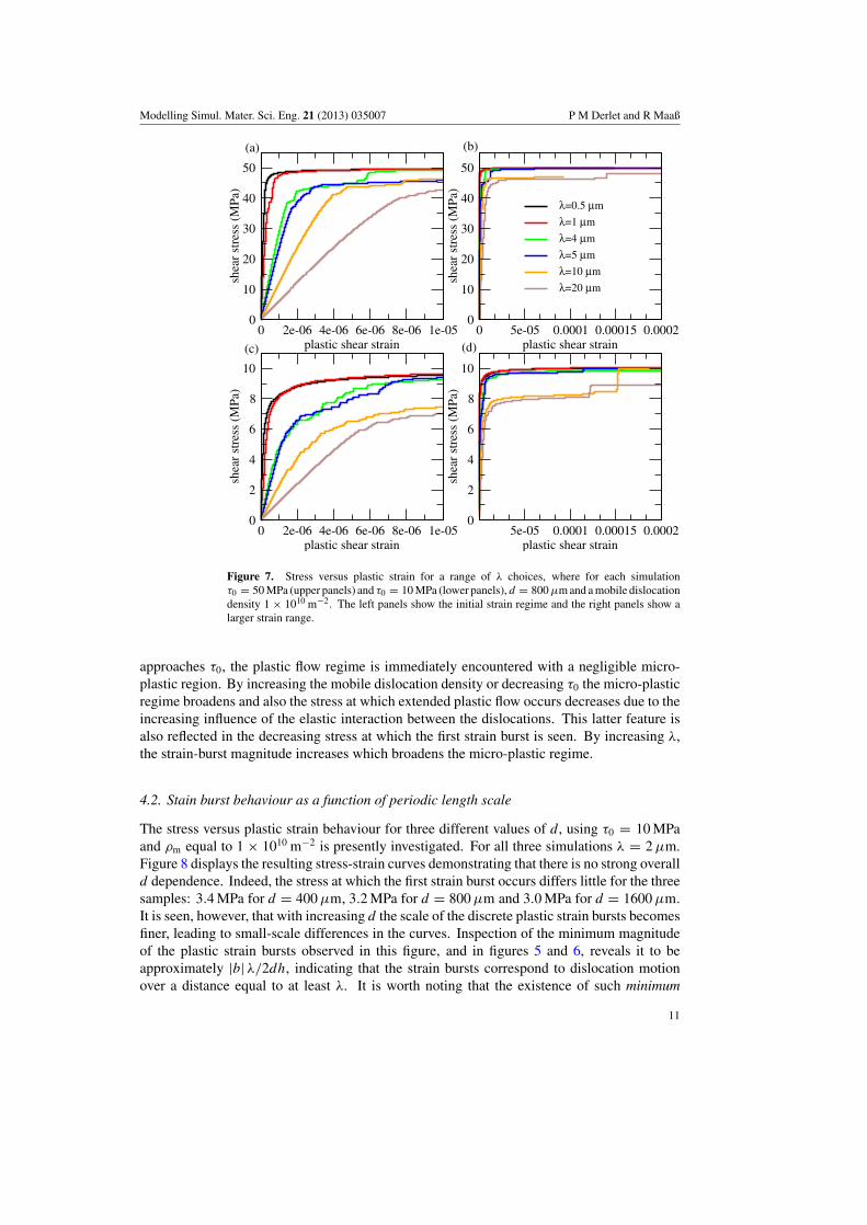
The remaining micro-structural variable that can be varied is the characteristic lengthscale of the sinusoidal stress field, λ. Figure 7 displays stress versus plastic strain curves asλ increases from λ = 0.5 µm to λ = 20 µm, with τ0 = 10 and 50 MPa, d = 800 µm andρm = 1 × 1010 m−2. Here a larger d was used to obtain a better statistical sample of thedislocation environment at the length scale of λ. The chosen dislocation density is similar tothat of figure 5 in which τ0 largely determined the flow stress. Inspection of figure 7 revealsthat with increasing λ the micro-plastic regime is broadened due to increasing strain burstmagnitudes with increasing λ. For small strain (figures 7(a) and (c)), it also appears thatthe flow stress regime occurs at a reduced stress (for increasing λ), however at larger strains(figures 7(b) and (d)) flow stresses approximately equal to τ0 are eventually reached. It isalso noted that with increasing λ the strain-burst magnitude increases. With decreasing τ0,the deviation of the curves away from τ0 is a stronger function of increasing λ resulting in asomewhat broader micro-plastic region.

The central properties of the present model are reflected in figures 5, 6 and 7. If thedislocation density is low enough or τ0 sufficiently high, then τ0 will primarily determine theshear-stress at which the extended plastic flow regime begins. In this limit, the internal shear-stress that each dislocation experiences is due to the sinusoidal stress field and when τapplied

10

Modelling Simul. Mater. Sci. Eng. 21 (2013) 035007 P M Derlet and R Maaß

0 2e-06 4e-06 6e-06 8e-06 1e-05plastic shear strain

0

10

20

30

40

50

shea

r st

ress

(M

Pa)

0 5e-05 0.0001 0.00015 0.0002plastic shear strain

0

10

20

30

40

50

shea

r st

ress

(M

Pa)

0 2e-06 4e-06 6e-06 8e-06 1e-05plastic shear strain

0

2

4

6

8

10

shea

r st

ress

(M

Pa)

5e-05 0.0001 0.00015 0.0002plastic shear strain

0

2

4

6

8

10

shea

r st

ress

(M

Pa)

λ=0.5 µm

λ=1 µm

λ=4 µm

λ=5 µm

λ=10 µm

λ=20 µm

(a) (b)

(c) (d)

Figure 7. Stress versus plastic strain for a range of λ choices, where for each simulationτ0 = 50 MPa (upper panels) and τ0 = 10 MPa (lower panels), d = 800 µm and a mobile dislocationdensity 1 × 1010 m−2. The left panels show the initial strain regime and the right panels show alarger strain range.

approaches τ0, the plastic flow regime is immediately encountered with a negligible micro-plastic region. By increasing the mobile dislocation density or decreasing τ0 the micro-plasticregime broadens and also the stress at which extended plastic flow occurs decreases due to theincreasing influence of the elastic interaction between the dislocations. This latter feature isalso reflected in the decreasing stress at which the first strain burst is seen. By increasing λ,the strain-burst magnitude increases which broadens the micro-plastic regime.

4.2. Stain burst behaviour as a function of periodic length scale

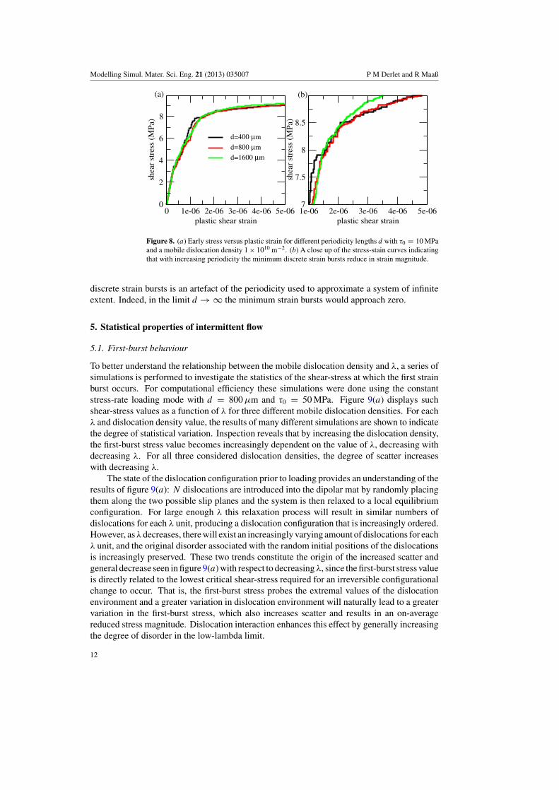
The stress versus plastic strain behaviour for three different values of d, using τ0 = 10 MPaand ρm equal to 1 × 1010 m−2 is presently investigated. For all three simulations λ = 2 µm.Figure 8 displays the resulting stress-strain curves demonstrating that there is no strong overalld dependence. Indeed, the stress at which the first strain burst occurs differs little for the threesamples: 3.4 MPa for d = 400 µm, 3.2 MPa for d = 800 µm and 3.0 MPa for d = 1600 µm.It is seen, however, that with increasing d the scale of the discrete plastic strain bursts becomesfiner, leading to small-scale differences in the curves. Inspection of the minimum magnitudeof the plastic strain bursts observed in this figure, and in figures 5 and 6, reveals it to beapproximately |b| λ/2dh, indicating that the strain bursts correspond to dislocation motionover a distance equal to at least λ. It is worth noting that the existence of such minimum

11

Modelling Simul. Mater. Sci. Eng. 21 (2013) 035007 P M Derlet and R Maaß

0 1e-06 2e-06 3e-06 4e-06 5e-06plastic shear strain

0

2

4

6

8

shea

r st

ress

(M

Pa)

d=400 µm

d=800 µm

d=1600 µm

1e-06 2e-06 3e-06 4e-06 5e-06plastic shear strain

7

7.5

8

8.5

shea

r st

ress

(M

Pa)

(a) (b)

Figure 8. (a) Early stress versus plastic strain for different periodicity lengths d with τ0 = 10 MPaand a mobile dislocation density 1 × 1010 m−2. (b) A close up of the stress-stain curves indicatingthat with increasing periodicity the minimum discrete strain bursts reduce in strain magnitude.

discrete strain bursts is an artefact of the periodicity used to approximate a system of infiniteextent. Indeed, in the limit d → ∞ the minimum strain bursts would approach zero.

5. Statistical properties of intermittent flow

5.1. First-burst behaviour

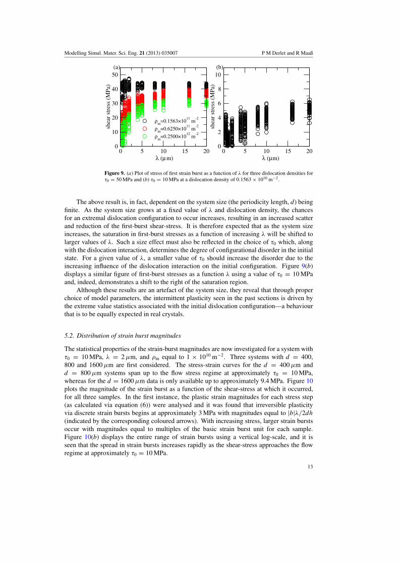
To better understand the relationship between the mobile dislocation density and λ, a series ofsimulations is performed to investigate the statistics of the shear-stress at which the first strainburst occurs. For computational efficiency these simulations were done using the constantstress-rate loading mode with d = 800 µm and τ0 = 50 MPa. Figure 9(a) displays suchshear-stress values as a function of λ for three different mobile dislocation densities. For eachλ and dislocation density value, the results of many different simulations are shown to indicatethe degree of statistical variation. Inspection reveals that by increasing the dislocation density,the first-burst stress value becomes increasingly dependent on the value of λ, decreasing withdecreasing λ. For all three considered dislocation densities, the degree of scatter increaseswith decreasing λ.

The state of the dislocation configuration prior to loading provides an understanding of theresults of figure 9(a): N dislocations are introduced into the dipolar mat by randomly placingthem along the two possible slip planes and the system is then relaxed to a local equilibriumconfiguration. For large enough λ this relaxation process will result in similar numbers ofdislocations for each λ unit, producing a dislocation configuration that is increasingly ordered.However, asλdecreases, there will exist an increasingly varying amount of dislocations for eachλ unit, and the original disorder associated with the random initial positions of the dislocationsis increasingly preserved. These two trends constitute the origin of the increased scatter andgeneral decrease seen in figure 9(a) with respect to decreasing λ, since the first-burst stress valueis directly related to the lowest critical shear-stress required for an irreversible configurationalchange to occur. That is, the first-burst stress probes the extremal values of the dislocationenvironment and a greater variation in dislocation environment will naturally lead to a greatervariation in the first-burst stress, which also increases scatter and results in an on-averagereduced stress magnitude. Dislocation interaction enhances this effect by generally increasingthe degree of disorder in the low-lambda limit.

12

Modelling Simul. Mater. Sci. Eng. 21 (2013) 035007 P M Derlet and R Maaß

0 5 10 15 20λ (µm)

0

10

20

30

40

50

shea

r st

ress

(M

Pa)

ρm

=0.1563×1011

m-2

ρm

=0.6250×1011

m-2

ρm

=0.2500×1012

m-2

0 5 10 15 20λ (µm)

0

2

4

6

8

10

shea

r st

ress

(M

Pa)

(b)(a)

Figure 9. (a) Plot of stress of first strain burst as a function of λ for three dislocation densities forτ0 = 50 MPa and (b) τ0 = 10 MPa at a dislocation density of 0.1563 × 1010 m−2.

The above result is, in fact, dependent on the system size (the periodicity length, d) beingfinite. As the system size grows at a fixed value of λ and dislocation density, the chancesfor an extremal dislocation configuration to occur increases, resulting in an increased scatterand reduction of the first-burst shear-stress. It is therefore expected that as the system sizeincreases, the saturation in first-burst stresses as a function of increasing λ will be shifted tolarger values of λ. Such a size effect must also be reflected in the choice of τ0 which, alongwith the dislocation interaction, determines the degree of configurational disorder in the initialstate. For a given value of λ, a smaller value of τ0 should increase the disorder due to theincreasing influence of the dislocation interaction on the initial configuration. Figure 9(b)displays a similar figure of first-burst stresses as a function λ using a value of τ0 = 10 MPaand, indeed, demonstrates a shift to the right of the saturation region.

Although these results are an artefact of the system size, they reveal that through properchoice of model parameters, the intermittent plasticity seen in the past sections is driven bythe extreme value statistics associated with the initial dislocation configuration—a behaviourthat is to be equally expected in real crystals.

5.2. Distribution of strain burst magnitudes

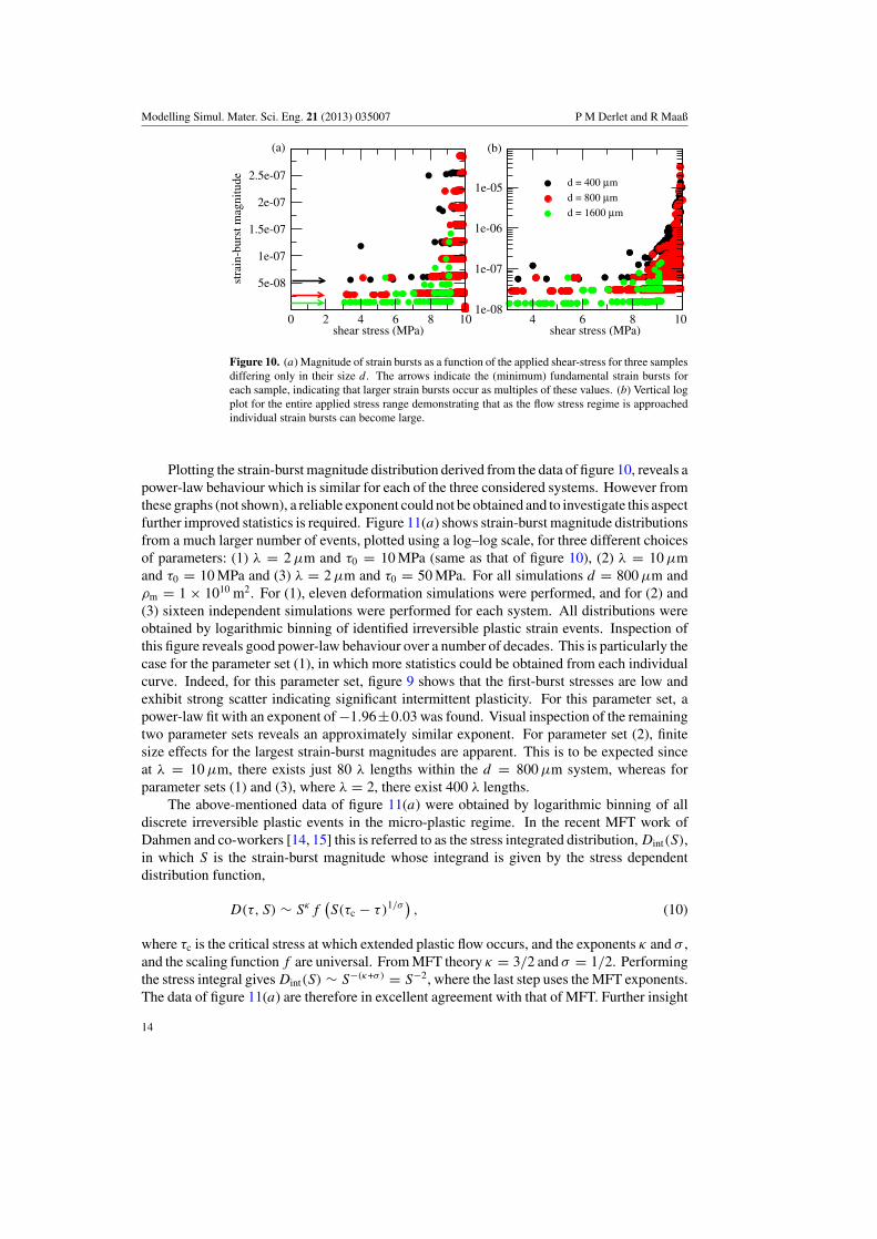
The statistical properties of the strain-burst magnitudes are now investigated for a system withτ0 = 10 MPa, λ = 2 µm, and ρm equal to 1 × 1010 m−2. Three systems with d = 400,800 and 1600 µm are first considered. The stress-strain curves for the d = 400 µm andd = 800 µm systems span up to the flow stress regime at approximately τ0 = 10 MPa,whereas for the d = 1600 µm data is only available up to approximately 9.4 MPa. Figure 10plots the magnitude of the strain burst as a function of the shear-stress at which it occurred,for all three samples. In the first instance, the plastic strain magnitudes for each stress step(as calculated via equation (6)) were analysed and it was found that irreversible plasticityvia discrete strain bursts begins at approximately 3 MPa with magnitudes equal to |b|λ/2dh

(indicated by the corresponding coloured arrows). With increasing stress, larger strain burstsoccur with magnitudes equal to multiples of the basic strain burst unit for each sample.Figure 10(b) displays the entire range of strain bursts using a vertical log-scale, and it isseen that the spread in strain bursts increases rapidly as the shear-stress approaches the flowregime at approximately τ0 = 10 MPa.

13

Modelling Simul. Mater. Sci. Eng. 21 (2013) 035007 P M Derlet and R Maaß

0 2 4 6 8 10shear stress (MPa)

5e-08

1e-07

1.5e-07

2e-07

2.5e-07

stra

in-b

urst

mag

nitu

de d = 400 µm

d = 800 µm

d = 1600 µm

4 6 8 10shear stress (MPa)

1e-08

1e-07

1e-06

1e-05

(a) (b)

Figure 10. (a) Magnitude of strain bursts as a function of the applied shear-stress for three samplesdiffering only in their size d. The arrows indicate the (minimum) fundamental strain bursts foreach sample, indicating that larger strain bursts occur as multiples of these values. (b) Vertical logplot for the entire applied stress range demonstrating that as the flow stress regime is approachedindividual strain bursts can become large.

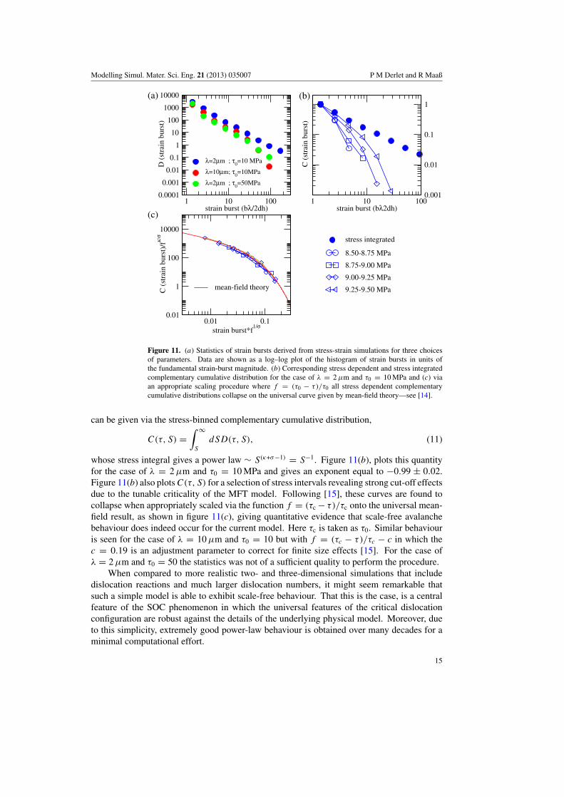
Plotting the strain-burst magnitude distribution derived from the data of figure 10, reveals apower-law behaviour which is similar for each of the three considered systems. However fromthese graphs (not shown), a reliable exponent could not be obtained and to investigate this aspectfurther improved statistics is required. Figure 11(a) shows strain-burst magnitude distributionsfrom a much larger number of events, plotted using a log–log scale, for three different choicesof parameters: (1) λ = 2 µm and τ0 = 10 MPa (same as that of figure 10), (2) λ = 10 µmand τ0 = 10 MPa and (3) λ = 2 µm and τ0 = 50 MPa. For all simulations d = 800 µm andρm = 1 × 1010 m2. For (1), eleven deformation simulations were performed, and for (2) and(3) sixteen independent simulations were performed for each system. All distributions wereobtained by logarithmic binning of identified irreversible plastic strain events. Inspection ofthis figure reveals good power-law behaviour over a number of decades. This is particularly thecase for the parameter set (1), in which more statistics could be obtained from each individualcurve. Indeed, for this parameter set, figure 9 shows that the first-burst stresses are low andexhibit strong scatter indicating significant intermittent plasticity. For this parameter set, apower-law fit with an exponent of −1.96±0.03 was found. Visual inspection of the remainingtwo parameter sets reveals an approximately similar exponent. For parameter set (2), finitesize effects for the largest strain-burst magnitudes are apparent. This is to be expected sinceat λ = 10 µm, there exists just 80 λ lengths within the d = 800 µm system, whereas forparameter sets (1) and (3), where λ = 2, there exist 400 λ lengths.

The above-mentioned data of figure 11(a) were obtained by logarithmic binning of alldiscrete irreversible plastic events in the micro-plastic regime. In the recent MFT work ofDahmen and co-workers [14, 15] this is referred to as the stress integrated distribution, Dint(S),in which S is the strain-burst magnitude whose integrand is given by the stress dependentdistribution function,

D(τ, S) ∼ Sκf(S(τc − τ)1/σ

), (10)

where τc is the critical stress at which extended plastic flow occurs, and the exponents κ and σ ,and the scaling function f are universal. From MFT theory κ = 3/2 and σ = 1/2. Performingthe stress integral gives Dint(S) ∼ S−(κ+σ) = S−2, where the last step uses the MFT exponents.The data of figure 11(a) are therefore in excellent agreement with that of MFT. Further insight

14

Modelling Simul. Mater. Sci. Eng. 21 (2013) 035007 P M Derlet and R Maaß

1 10 100strain burst (bλ/2dh)

0.0001

0.001

0.01

0.1

1

10

100

1000

10000

D (

stra

in b

urst

)λ=2µm ; τ

0=10 MPa

λ=10µm; τ0=10MPa

λ=2µm ; τ0=50MPa

1 10 100strain burst (bλ2dh)

0.001

0.01

0.1

1

C (

stra

in b

urst

)

stress integrated

8.50-8.75 MPa

8.75-9.00 MPa

9.00-9.25 MPa

9.25-9.50 MPa

0.01 0.1strain burst*f

1/σ

0.01

1

100

10000

C (

stra

in b

urst

)/fκ/

σ

mean-field theory

(a) (b)

(c)

Figure 11. (a) Statistics of strain bursts derived from stress-strain simulations for three choicesof parameters. Data are shown as a log–log plot of the histogram of strain bursts in units ofthe fundamental strain-burst magnitude. (b) Corresponding stress dependent and stress integratedcomplementary cumulative distribution for the case of λ = 2 µm and τ0 = 10 MPa and (c) viaan appropriate scaling procedure where f = (τ0 − τ)/τ0 all stress dependent complementarycumulative distributions collapse on the universal curve given by mean-field theory—see [14].

can be given via the stress-binned complementary cumulative distribution,

C(τ, S) =∫ ∞

S

dSD(τ, S), (11)

whose stress integral gives a power law ∼ S(κ+σ−1) = S−1. Figure 11(b), plots this quantityfor the case of λ = 2 µm and τ0 = 10 MPa and gives an exponent equal to −0.99 ± 0.02.Figure 11(b) also plots C(τ, S) for a selection of stress intervals revealing strong cut-off effectsdue to the tunable criticality of the MFT model. Following [15], these curves are found tocollapse when appropriately scaled via the function f = (τc − τ)/τc onto the universal mean-field result, as shown in figure 11(c), giving quantitative evidence that scale-free avalanchebehaviour does indeed occur for the current model. Here τc is taken as τ0. Similar behaviouris seen for the case of λ = 10 µm and τ0 = 10 but with f = (τc − τ)/τc − c in which thec = 0.19 is an adjustment parameter to correct for finite size effects [15]. For the case ofλ = 2 µm and τ0 = 50 the statistics was not of a sufficient quality to perform the procedure.

When compared to more realistic two- and three-dimensional simulations that includedislocation reactions and much larger dislocation numbers, it might seem remarkable thatsuch a simple model is able to exhibit scale-free behaviour. That this is the case, is a centralfeature of the SOC phenomenon in which the universal features of the critical dislocationconfiguration are robust against the details of the underlying physical model. Moreover, dueto this simplicity, extremely good power-law behaviour is obtained over many decades for aminimal computational effort.

15

Modelling Simul. Mater. Sci. Eng. 21 (2013) 035007 P M Derlet and R Maaß

6. Discussion

The simulations of section 4 demonstrate that two dominant factors control the characteristicstress scale of the stress-strain curve. These are the choice of τ0 and the mobile dislocationdensity. Figures 5 and 6 demonstrate that τ0 sets an upper stress limit for extended plastic flowto occur. This upper limit is approached when the mobile dislocation density is sufficiently lowthat the sinusoidal stress field is the dominant contribution to the stress field each dislocationfeels. By increasing the mobile dislocation content, the characteristic shear-stress scale reducesdue to the increasing role of the internal stress fields arising from the elastic interaction betweendislocations. At the same time a broadening of the micro-plastic regime is observed, whichis very much a general property of micro-yielding, where a greater number of mobile edgedislocations correlates with larger measurable plastic strain [45]. Figures 7–9 demonstrate theeffect of λ (and d) on the stress-strain curve is somewhat subtler. The choice of λ influences theinitial configuration of the mobile dislocation population, thereby affecting the statistics of thestress at which the first strain-burst occurs and also the way in which the extended plastic flowregime is reached. Figure 11 shows, however, that the statistics of the strain-burst magnitudeis insensitive to all three discussed parameters, reflecting the universality of SOC with respectto micro-structural details.

How shall one quantitatively interpret the imposed sinusoidal stress field? In a real materialthat is nominally free of dislocation structures, some type of length scale will naturally emergeas a function of macroscopic plastic strain due to the evolution of a growing and interactingdislocation structure that eventually leads to the phenomenon of patterning [46]. Althoughpatterning is a term predominantly referring to the effects of latter stage II and III hardeningregimes, the emergence of micro-structure length scales is expected to occur at all stagesof plasticity ranging from slip, dipole and eventually cellular patterns [36, 47, 48]. In fact, amicro-structural length scale can equally well be defined for an undeformed as-grown material,where the mean dislocation spacing can be used to describe the initially present internal stressfluctuations—a view point that is central to the early work of Tinder and co-workers [1, 2]. Fromthis perspective the imposed sinusoidal stress field, can be viewed as the simplest realizationof the internal stress field arising from such a structure.

In the present model this stress field is time independent, implying that it is constructed bythat part of the dislocation population that is immobile, with the explicit dislocations and theirdynamics, arising from the (much smaller) mobile component of the dislocation population.Thus a typical loading simulation can be seen as the deformation of a model material that hasa particular sample preparation or deformation history characterized by τ0 and λ, and a mobiledislocation density that is only a small part of the total dislocation density.

Much past work exists concerning the emergence of internal stress and length scales as afunction of deformation history. In early work on the theory of cell formation, two relationshipshave emerged in which the total evolving dislocation density, ρtotal, plays a central role. They are

τmaterial

G∝ b

√ρtotal (12)

and

λmaterial ∝ 1√ρtotal

, (13)

where G is a representative (not necessarily pure) shear modulus and b the Burgers vectormagnitude. In the above, τmaterial is the evolving flow stress of the material and λmaterial is anevolving internal length scale that can be referred to as a cell size. The first expression has

16

Modelling Simul. Mater. Sci. Eng. 21 (2013) 035007 P M Derlet and R Maaß

its earliest origins in a Taylor hardening picture in which the total dislocation density is seenas an immobile forest dislocation population. The second equation has its theoretical originsin the early work of Holt [49] who derived it for a dipolar population of screw-dislocations,showing that a uniform arrangement was unstable to fluctuations with one such length scaledominating, characterized by equation (13). This length scale, which could be related to afixed self-screening distance of the dislocation network, was postulated to reflect an emergingcell size. The approach was based on an energy minimization principle; however, due todislocation reactions, the more modern viewpoint is that the dynamics of cell formation lies ina statistical process involving dislocation reactions and that the screening length, and thereforecell-size, is an evolving variable [48].

Thus, the model parameter λ has a direct counterpart in cell formation theory, λmaterial,which can represent quite generally, a mean-free path for a mobile dislocation, a dipolarscreening length or a well evolved cell length scale. Moreover, since an unloading/loadingcycle will generally return a system to the flow stress before unloading, and that the presentsimulations have shown that the flow stress is partly controlled by τ0, τ0 should be in someway related to τmaterial. From this perspective, τ0 and λ are parameters that are not entirelyindependent from each other. In fact, equations (12) and (13) express that the cell size decreasesinversely as a function of flow stress, a well known experimental observation that is referredto as ‘similitude’ [36].

Although similitudity is generally confirmed by experiment, some experimental work doespresent a more complicated picture. Early tensile/TEM work on tapered Cu single crystalsfinds an initially broad distribution of cell sizes that narrows and shifts to small lengths withincreasing flow stress [50]. This result suggests that a single structural length scale might notalways be a good statistical description of the evolving micro-structure. Indeed, more modernviewpoints, in which dislocation structure evolution is a non-equilibrium process [51], tend tosuggest a distribution of emerging length scales leading to a scale-free fractal-like structure.Although such micro-structures have been quantitatively established by TEM investigations oflatter-stage hardened single crystals of Cu [52, 53], their existence is not universal, dependingstrongly on material type and deformation history. The current work does not address thisaspect. More general forms of an inhomogeneous internal stress field that capture such scale-free micro-structural features can be envisioned.

Whilst the dipolar mat geometry in an external field offers a platform with which tostudy the depinning transition and more generally the transition to extended plastic flow, whencomparing to experiment, careful consideration has to be given to its regime of applicability.To do this, a typical simulation of sections 4 and 5 is now broadly summarized. Upon choosingnumerical values for all model parameters, the N dislocations are introduced to the systemvia a distribution of random positions. This unstable configuration is then relaxed to a localminimum energy in which the forces on each dislocation are below a small threshold value.The deformation simulation is then begun using one of the three loading modes of section 3.As the stress increases, intermittent plasticity increasingly occurs until a stress is reached atwhich extended and overlapping strain events occur, which in the previous sections has looselybeen referred to as the plastic flow regime.

It is important to emphasise that no attempt has been made to obtain the global energyminimum of the starting configuration. Such an initial state turns out to play a crucial role inthe observed properties of the model, since many high-energy configurations will exist, and itis these that dominate the early stages of plasticity. As a deformation simulation proceeds, suchhigh-energy configurations structurally transform eventually leading to a plastic flow regimeand often to the homogenization of the dislocation configuration. In other words, the extendedplastic flow regime should be considered to be outside the applicability regime of the present

17

Modelling Simul. Mater. Sci. Eng. 21 (2013) 035007 P M Derlet and R Maaß

model when a comparison to experiment is made, or equivalently, the present model is onlysuitable for the study of the micro-plastic regime of the stress-strain curve.

The rational behind the use of an initial high-energy dislocation configuration originatesfrom the assumption that the explicit dislocation population of the model represents onlythe mobile dislocation network, which constitutes only a small part of the true population.Thus, in the same way as τ0 and λ characterize the sample preparation or deformation historyof the model material, so does the initial high-energy (explicit) mobile dislocation content.This is quite compatible from the perspective of SOC in which the dislocation structurereaches a critical configuration that is far from equilibrium, and that structural rearrangementscorrespond to the system transforming from one SOC state to another. By construction, thatpart mediating the structural transformation will be the current mobile dislocation content.The central simplification of the present model is that it separates the mobile and immobilepopulations, associating the former to an explicit mobile dislocation content that representsthe non-equilibrium component of the network, and relegating the latter to an effectivestatic internal stress field. That this internal stress field is unchanging and that the sameexplicit mobile dislocation population exists as a function of strain for the entire deformationsimulation, is of course different from a real material, where the structure evolves with strain,and at any particular non-negligible strain interval, quite different dislocations might constitutethe mobile dislocation population. This again emphasizes that the present model should onlybe applied to the micro-plastic regime, where significant structural evolution is minimal.

Experimental evidence for a lack of structural evolution in the mico-plastic regime is bestseen in low amplitude cyclic deformation experiments of FCC metals, in which the plasticstrain per cycle can be as low as 10−5 leading to significant changes in load stress andinternal length scale only after the occurrence of several tens-to-hundreds of thousands ofcycles [54, 55]. It is further noted, that documented experimental studies of micro-plasticityat room temperature primarily report on movements of edge or non-screw type dislocations,whereas a clear increase in dislocation density or the formation of dislocation structures as aresult of multiplication remains absent [39, 40, 56]. In the bulk case there are exceptions tothis trend where in the case of a work-hardened Al–Mg alloy which exhibits dynamic strainaging, emerging structural length scales were already detected in the micro-plastic regime [13]using high-resolution extensometry methods [12, 57, 58].

The results of section 5.2 demonstrate that the developed model exhibits power-lawbehaviour in the distribution of strain-burst magnitudes, and thus the scale-free avalanchephenomenon seen in experiments, either via the stress-strain curve of micro-compressiontests [6, 7] or via in situ acoustic emission experiments [18, 19], and in simulation, via two-or three-dimensional DD simulations in which the entire network is represented by an explicitdislocation population and individual dislocation reaction mechanisms are taken into account.That such a simple model can admit scale-free behaviour is connected to the dependence ofthe intermittent plasticity on the extremal configurations of the explicit dislocation population.This was directly seen in the statistics of the first-burst shear-stress and also the distributionof strain-burst magnitudes, where with a large enough increase of λ (say from 2 to 10 µm)the first-burst statistics changes from being dominated by extreme value statistics to that beingdominated by the statistics of the most probable (figure 9(b)) corresponding to an increasedpresence of cut-off effects in the statistics of strain-burst magnitudes (figure 11(a)). This isa natural result of the observation that quantities that depend on extreme value statistics canexhibit power-law behaviour in their distributions, emphasizing a connection with SOC thatis related to only the mobile dislocation population being in a non-equilibrium state and notto the characteristics of the present simplified immobile dislocation network—a manifestationof a scenario referred to as ‘nearly critical’ or ‘robust critical’ [34].

18

Modelling Simul. Mater. Sci. Eng. 21 (2013) 035007 P M Derlet and R Maaß

7. Concluding remarks

A simplified two-dimensional dislocation modelling framework has been introduced in whichthe explicit interacting dislocation population, constrained to a simple dipolar mat geometry,represents only the mobile dislocation density component of the total dislocation density, andthe much larger immobile dislocation population is described by a static internal sinusoidalshear-stress field defined by an internal shear-stress amplitude and wavelength. Thesemodel parameters, along with the initial non-equilibrium explicit mobile dislocation contentcharacterize either the deformation or sample preparation history of the model material.Because of the static nature of the internal field and the lack of dislocation-dislocation reactions,upon loading, the present model is restricted to the micro-plastic region of the stress-straincurve, and therefore to a deformation regime for a given material that involves negligiblestructural evolution. Despite the simplicity of the model and the restriction to the micro-plastic regime, the deformation behaviour exhibits a rich variety of properties as a functionof the model parameters. In particular, intermittent plasticity is observed whose strain-burstmagnitude distribution exhibits scale-free avalanche behaviour.

Acknowledgments

PMD wishes to thank PD Ispanovity for useful discussions. RM gratefully acknowledges thefinancial support of the Alexander von Humboldt Foundation and his host GM Pharr, as wellas institutional support by JR Greer at Caltech.

Appendix. Periodic boundary condition treatment

Due to the long range nature of equation (2), all image contributions must be taken into accountfor the correct treatment of the periodic boundary conditions along the dipolar mat direction.The force per unit dislocation length on a dislocation n (at position (xn, yn)) due to a dislocationn′ (at position (xn′ , yn′)) and it’s images, is given by the infinite summation:

fx,nn′ = Gbx,nbx,n′

2π(1 − ν)

∞∑k=−∞

(xn − (xn′ − kd))((xn − (xn′ − kd))2 − (yn − yn′)2)

((xn − (xn′ − kd))2 + (yn − yn′)2)2. (A1)

Due to the periodic boundary condition being one-dimensional, an analytic solution to theabove summation can be found. To do this, the summation in equation (A1) is rewritten as

limk′→∞

k′∑k=−k′−1

(�x + kd)((�x + kd)2 − �y2)

((�x + kd)2 + �y2)2, (A2)

where �x = xn − xn′ and �y = yn − yn′ and 0 < �x < d/2.The above summation is explicitly convergent for all values of k′, and may be evaluated

analytically in terms of poly-gamma functions. This is achieved by first expressing thesummand in equation (A2) as an irreducible partial fraction:

1

2(�x − ı�y + kd)+

1

2(�x + ı�y + kd)+

ı�y

2(�x − ı�y + kd)2− ı�y

2(�x + ı�y + kd)2.

(A3)

In this form, the summation to a finite k′ may be straightforwardly obtained via a known seriesexpansion of poly-gamma functions [59], giving

k′∑k=−k′−1

1

(z + kd)= − 1

d

[φ(0)

(−1 − k′ +

z

d

)− φ(0)(1 + k′ +

z

d)]

(A4)

19

Modelling Simul. Mater. Sci. Eng. 21 (2013) 035007 P M Derlet and R Maaß

-40 -20 0 20 40dislocation separation (µm)

-1.5

-1

-0.5

0

0.5

1

1.5

rest

orin

g st

ress

(M

Pa)

h=10 µm, ρ m

=1.000×1010

m-2

h=5 µm, ρm

=4.000×1010

m-2

h=2.5 µm, ρm

=1.600×1111

m-2

h=1.25 µm, ρ m

=6.400×1011

m-2

h=0.625 µm, ρ m

=2.560×1012

m-2

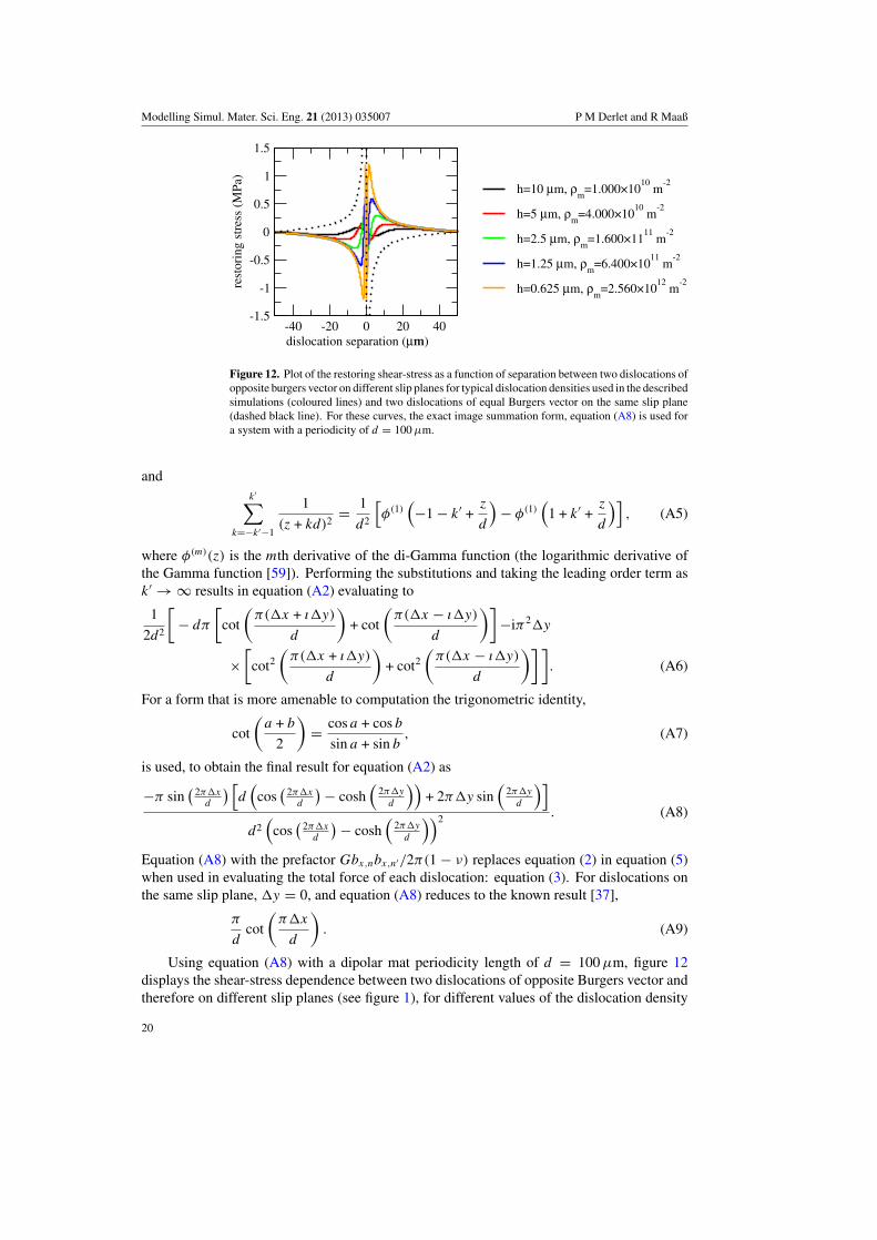
Figure 12. Plot of the restoring shear-stress as a function of separation between two dislocations ofopposite burgers vector on different slip planes for typical dislocation densities used in the describedsimulations (coloured lines) and two dislocations of equal Burgers vector on the same slip plane(dashed black line). For these curves, the exact image summation form, equation (A8) is used fora system with a periodicity of d = 100 µm.

andk′∑

k=−k′−1

1

(z + kd)2= 1

d2

[φ(1)

(−1 − k′ +

z

d

)− φ(1)

(1 + k′ +

z

d

)], (A5)

where φ(m)(z) is the mth derivative of the di-Gamma function (the logarithmic derivative ofthe Gamma function [59]). Performing the substitutions and taking the leading order term ask′ → ∞ results in equation (A2) evaluating to

1

2d2

[− dπ

[cot

(π(�x + ı�y)

d

)+ cot

(π(�x − ı�y)

d

)]−iπ2�y

×[

cot2

(π(�x + ı�y)

d

)+ cot2

(π(�x − ı�y)

d

)] ]. (A6)

For a form that is more amenable to computation the trigonometric identity,

cot

(a + b

2

)= cos a + cos b

sin a + sin b, (A7)

is used, to obtain the final result for equation (A2) as

−π sin(

2π�xd

) [d

(cos

(2π�x

d

) − cosh(

2π�y

d

))+ 2π�y sin

(2π�y

d

)]

d2(

cos(

2π�xd

) − cosh(

2π�y

d

))2 . (A8)

Equation (A8) with the prefactor Gbx,nbx,n′/2π(1 − ν) replaces equation (2) in equation (5)when used in evaluating the total force of each dislocation: equation (3). For dislocations onthe same slip plane, �y = 0, and equation (A8) reduces to the known result [37],

π

dcot

(π�x

d

). (A9)

Using equation (A8) with a dipolar mat periodicity length of d = 100 µm, figure 12displays the shear-stress dependence between two dislocations of opposite Burgers vector andtherefore on different slip planes (see figure 1), for different values of the dislocation density

20

Modelling Simul. Mater. Sci. Eng. 21 (2013) 035007 P M Derlet and R Maaß

and thus different h. Inspection of this figure reveals the short range structure to be similarto that of the bare interaction given by equation (2) in section 2, whereas at larger distancesthe interaction correctly limits to zero at ±d/2. In this figure the chosen numerical values ofthe mobile dislocation density (where h = 1/

√ρm) will be typical of those used in this work.

Inspection of this figure reveals that for the highest dislocation density, the restoring stressis at most of the order of 1 MPa and thus small when compared to the considered values ofτ0, and also typical values of the stress associated with intra-slip-plane dislocation interactionat sub-micrometre distances (see the dashed line in figure 12, which displays the restoringshear-stress between two dislocations of the same Burgers vector on the same slip plane). Toinvestigate the regime in which the two slip planes strongly interact, higher mobile dislocationdensities would need to be considered or a different relationship between h and the dislocationdensity taken.

References

[1] Tinder R F and Washburn J 1964 Acta. Metall. 12 129[2] Tinder R F and Trzil J P 1973 Acta Metall. 21 975[3] Neuhauser H 1983 Slip line formation and collective dislocation motion Dislocations in Solids vol 6 ed F R N

Nabarro (Amsterdam: Elsevier) p 319[4] Uchic M D, Dimiduk D K, Florando J N and Nix W D 2004 Science 305 986[5] Greer J R, Oliver W C and Nix W D 2005 Acta Mater. 53 1821[6] Dimiduk D K, Woodward C, LeSar R and Uchic M D 2006 Science 312 1188[7] Dimiduk D K, Nadgorny E M, Woodward C, Uchic M D and Shade P A 2010 Phil. Mag. 90 3621[8] Volkert C A and Lilleodden E T 2006 Phil. Mag. 86 13[9] Maaß R and Uchic M D 2012 Acta Mater. 60 1027

[10] Maass R, Meza L, Gan B, Tin S, Greer J R 2012 Small 8 1869[11] Zaiser M, Schwerdtfeger J, Schneider A S, Frick C P, Clark B G, Gruber P A and Arzt E 2008 Phil. Mag. 88 3861[12] Fressengeas C, Beaudoin A J, Entemeyer D, Lebedkina T, Lebyodkin M and Taupin V 2009 Phys. Rev. B

79 014108[13] Mudrock R N, Lebyodkin M A, Kurath P, Beaudoin A J and Lebedkinac T A 2011 Scr. Mater. 65 1093[14] Dahmen K A, Ben-Zion Y and Uhl J T 2009 Phys. Rev. Lett. 102 175501[15] Friedman N, Jennings A T, Tsekenis G, Kim J-Y, Tao M, Uhl J T, Greer J R and Dahmen K A 2012 Phys. Rev.

Lett. 109 095507[16] Sethna J P, Dahmen K A and Myers C R 2001 Nature 410 242[17] Sun B A, Yu H B, Jiao W, Bai H Y, Zhao D Q and Wang W H 2010 Phys. Rev. Lett. 105 035501[18] Miguel M-C, Vespignani A, Zapperi S, Weiss J and Grasse J R 2001 Nature 410 667[19] Weiss J and Marsan D 2003 Science 299 89[20] See for example, Nabarro F R N and Hirth J (ed) 2002 Dislocations in Solids vol 11 (Amsterdam: Elsevier)[21] Amodeo R J and Ghoniem N M 1990 Phys. Rev. B 41 6958

Amodeo R J and Ghoniem N M 1990 Phys. Rev. B 41 6968[22] Devincre B and Pontikis V 1993 Mater. Res. Soc. Symp. Proc. 291 555[23] Fournet R and Salazar J M 1996 Phys. Rev. B 53 6283[24] Bako B, Groma I, Gyorgyi G, Zimanyi G 2006 Comput. Mater. Sci. 38 22[25] Van der Giessen E and Needleman A 1995 Modelling Simul. Mater. Sci. Eng. 3 689[26] Ispanovity P D, Groma I, Hoffelner W and Samaras M 2011 Modelling Simul. Mater. Sci. Eng. 19 045008[27] Deshpande V S, Needleman A and Van der Giessen E 2005 J. Mech. Phys. Solids 53 2661[28] Ispanovity P D, Groma I, Gyorgyi G, Csikor F F and Weygand D 2010 Phys. Rev. Lett. 105 085503[29] Weygand D, Friedman L H, Van der Giessen E and Needleman A 2002 Modelling Simul. Mater. Sci. Eng. 10 437[30] Bulatov V V and Cai W 2006 Computer Simulations of Dislocations (Oxford Series on Materials Modelling)

ed A P Sutton and R E Rudd (Oxford: Oxford University Press)[31] Csikor F F, Motz C, Weygand D, Zaiser M and Zapperi S 2007 Science 318 251[32] Rao S I, Dimiduk D M, Parthasarathy T A, Uchic M D, Tang M, Woodward C 2008 Acta. Mater. 56 3245[33] Devincre B, Hoc T and Kubin L 2009 Science 320 1745[34] Zaiser M 2006 Adv. Phys. 55 185[35] Bak P, Tang C and Wiesenfeld K 1987 Phys. Rev. Lett. 59 381

21

Modelling Simul. Mater. Sci. Eng. 21 (2013) 035007 P M Derlet and R Maaß

[36] Kuhlmann-Wilsdorf D 2002 The LES Theory of Solid Plasticity Dislocations in Solids vol 11 ed F R N Nabarroand J Hirth (Amsterdam: Elsevier) p 211

[37] Moretti P, Miguel M-Carmen, Zaiser M and Zapperi S 2004 Phys. Rev. B 69 214103[38] Leoni F and Zapperi S 2009 Phys. Rev. Lett. 102 115502[39] Young F W 1961 J. Appl. Phys. 32 1815[40] Vellaikal G 1969 Acta Metall. 17 1145[41] Hansen N and Kuhlmann-Wilsdorf D 1986 Mater. Sci. Eng. 81 141[42] Hull D and Bacon D J 2001 Introduction to Dislocations (Oxford: Butterworth Heinemann) chapter 4.6[43] See chapter 10.3 of [42].[44] Devincre B 1993 These de Doctorat (Paris XI Orsay)[45] Abel A 1973 Acta Metall. 21 99[46] Argon A S 2008 Strengthening Mechanisms in Crystal Plasticity (Oxford Series on Materials Modelling) ed A

P Sutton and R E Rudd (Oxford: Oxford University Press)[47] Mughrabi H 1983 Acta Metall. 31 1367[48] Kubin L P and Canova G 1992 Scri. Metall. Mater. 27 957[49] Holt D L 1970 J. Appl. Phys. 41 3197[50] Prinz F and Argon A S 1980 Phys. Status Solidi a 57 741[51] Hahner P 1996 Acta Mater. 44 2345[52] Hahner P, Bay K and Zaiser M 1998 Phys. Rev. Lett. 81 2470[53] Zaiser M, Bay K and Hahner P 1999 Acta Mater. 47 2463[54] Mughrabi H 1978 Mater. Sci. Eng. 33 207[55] Basinski Z S and Basinski S J 1992 Prog. Mater. Sci. 36 89[56] Koppenaal T J 1963 Acta Metall. 11 86[57] Roth A, Lebedkina T A, Lebyodkin M A 2012 Mater. Sci. Eng. A 539 280[58] Lebyodkin M A, Lebedkina T A, Roth A and Allain S 2012 Acta Phys. Pol. A 122 478[59] Abramowitz M and Stegun I A (ed) 1972 Handbook of Mathematical Functions with Formulas, Graphs, and

Mathematical Tables (New York: Dover) pp 258–60

22