Micro-based Participation Elasticities:New International Evidence∗

Olivier Bargain1,2 Herwig Immervoll2,3 Eric Sommer2,4

1University Aix-Marseille2IZA Bonn

3OECD4University Cologne

October 1, 2015

!!! Work in Progress - Please do not quote !!!

Abstract

This paper provides estimates on the extensive elasticity of labor supply for17 OECD countries for the period 2001 to 2012. Comparability across countriesis achieved by applying a uniform empirical framework, exploiting tax-benefit andwage changes between demographic subgroups. Our findings confirm previous evi-dence on the magnitude of participation elasticities, but go beyond existing studiesby providing a richer picture its interaction with institutional confounders. We dofind evidence for differential responsiveness of workers along the business cycle andfor different minimum wage levels.

JEL Classification: H21, H55, J22Keywords: labor supply elasticity, taxation, design of welfare systems

∗Corresponding author: Eric Sommer, (sommer@iza.org), IZA Bonn, P.O. Box 7240, 53072 Bonn,Germany, Tel.: +49(0)228 3894–419, Fax: +49(0)228 3894–510. We thank Linda Richardson, Sean Gib-son, Karinne Logez and Pascal Marianna for data provision and assistance. We also thank SebastianKonigs and Andrea Bassanini for valuable suggestions.

1 Introduction

Individual employment decisions are considered to be strongly shaped by the design of

tax-benefit systems, thereby explaining employment performances across countries to a

considerable extent (Prescott, 2004). The magnitude of this effect is of high relevance for

policy-makers in order to assess the employment impact of tax-benefit reforms (Immervoll

et al., 2007). From a theoretical perspective, this margin is of major importance for the

efficiency costs of taxation (Saez, 2001). As a consequence, a vast empirical literature on

labor supply elasticities has emerged (Keane, 2011).

Despite this large literature, only a handful of studies provide comparable micro-based

estimates for several countries by applying a unified empirical approach. Bargain et al.

(2014) estimate a structural discrete-choice model, combined with a tax-benefit calculator

and obtain labor supply elasticities for 17 EU countries and the US. The underlying

data represent one single cross-section respectively. With a complementary approach,

Jantti et al. (2015) exploit variation between demographic groups to identify labor supply

elasticities on the micro and macro level for 13 OECD countries.

We contribute to this literature in several aspects. While our approach also applies

a comparable empirical framework, our data span OECD countries over the continuous

period from 2001 to 2012. As labor supply elasticities have been found to change over

the long term (Heim (2007), Blau and Kahn (2007)), the identification of a structural

parameter is probably more reliable if focused on a narrower time window. We cover em-

ployment behavior and tax-benefit rules from North America, Southern Europe, Central

Europe and transition economies alike. Our identification approach builds on Blundell

et al. (1998b) exploiting variation in taxes and wages across demographic subgroups.

We test the sensitivity of our results by varying the time period for the identification,

thus also uncovering potential differences in behavioral strengths before and after the

Great Recession. The main contribution of this paper is to go beyond ’traditional’ micro-

based estimates on labor supply by providing an analysis of interactions of individual

labor supply with economic and institutional confounders. These encompass indicators

for the business-cycle, active labor market policies (ALMP) and the level of the minimum

wage. Our findings may yield implications for future tax-benefit reforms. They shed light

on how broadly certain policies can be applied. It could be that particular countries have

certain institutional or cultural characteristics that ask for specific policy responses that

might not be appropriate in other contexts.

Contrary to previous studies, we concentrate solely on the extensive margin of labor

supply, being more relevant than the hours margin. One common explanation for this

phenomenon is that tax changes are usually too small to induce behavioral adjustments;

either because workers face adjustment costs or because of limited awareness of the tax

rate change Chetty (2012). Moreover, the extensive margin is the critical one for the

optimal design of in-work policies (Immervoll et al., 2007).

1

The paper is structured as follows. Section 2 describes our data base, as well as our

concept for the work incentive. Section 3 explains the estimation strategy, while section

4 presents the results. Section 5 concludes and discusses policy implications.

2 Data

Employment For European countries, we rely on the European Labor Force Surveys

(EU-LFS). It is a comprehensive household survey, which is nowadays conducted in more

than 30 European countries and coordinated by Eurostat. In the early 2000s, its sur-

vey design switched from a snapshot in spring to a continuous sampling over the whole

year. It serves as reference for the officially published employment and unemployment

rates. The EU-LFS is delivered in two formats, as quarterly and annual sample. For

our analysis, we use the annual samples. Although they regularly bear fewer observa-

tions than the quarterly samples, only these contain the so-called ’structural variables’

on personal relations within the household.1 For the US, we rely the Current Population

Survey (CPS). Our outcome variable of interest is the employment status, which is defined

following ILO standards. Apart from persons in paid employment and self-employment,

this encompasses workers temporarily not at work for reasons such as illness, maternity

leave, vacation, strike, educational leave. In order to net out effects from transition from

education and into retirement, we limit the sample to prime-aged workers between 25

and 54 years. Following common practice, we exclude self-employed persons, as their

employment behavior arguably follows a different rationale than that of employees, which

implies different responses to incentives induced by the tax-benefit system.

Work Incentives A comprehensive measure on the monetary employment incentive

needs to account for tax and contribution payments and withdrawal of earnings-related

transfers when entering the labor market from inactivity I into Employment E. We

hence apply the Participation Tax Rate (PTR)(Immervoll et al., 2007), which is defined

as follows:

PTR = τ = 1 − ∆ynet∆ygross

= 1 − yEnet − yInetyEgross − yIgross

(1)

τ has to be interpreted as the share of gross income that is taxed away upon entering

employment (Carone et al., 2004). For the calculation, we assume a transition from zero

weekly hours to country-specific full-time work. Housing benefits are not considered in

the calculations, as they as are hard to assess accurately due to within-country variation

in housing costs. Transitory benefits, such as temporary unemployment benefits, are also

not considered. This accounts for the fact that the planning horizon of an individual may

be longer than the limited time of benefit payment. In this case, participation tax rates

1 This information is generally not available for Denmark, Switzerland and Norway. For Finland, areduced special sample was used.

2

based on short-term considerations may be too high (Pestel and Bartels, 2015).

The assignment of an individual PTR in the micro-data constitutes a challenge on its

own, as the EU-LFS does not contain information individual earnings yEgross. We hence

have to rely on auxiliary sources. We compute annual mean earnings by age group (25-

34, 35-44,45-55), obtained education and sex from national surveys.2 In the next step,

we obtain net income in and out of employment from the OECD TaxBenefit Calculator.

Gross income when not working is either zero for singles or corresponds to the earnings

of the spouse. The calculation accounts for family background, i. e. marital status,

employment status and qualification of the spouse and presence of children, yielding the

individual PTR.3 Persons in households with more than three adults and with non-

married partners are not assigned a PTR and are hence excluded from the analysis.

For workers in these households, a clear-cut classification as single or couple household

cannot be done. The OECD TaxBenefit Calculator contains policy parameters for all

OECD countries since 2001.

The selection of the estimation sample is ultimately driven by data availability and

asks for sufficient time coverage by Labor Force Survey and TaxBenefit Calculator at

the same time. Moreover, we abstain from including small sample countries such as

Luxembourg, Estonia and Slovenia, as group employment rates are very volatile due to

small sample sizes. Table 4 in the Appendix gives an overview about the sample sizes by

country and year.

3 Empirical Approach

Identifying the elasticity of labor supply is known to be associated with several empirical

challenges (Keane, 2011).4 Among these are unobserved tastes for work, endogeneity of

the tax rate and measurement error in wages. One way to account for unobserved tastes

for work is a Grouping Estimator, as suggested by Blundell et al. (1998a). It exploits

variation in working hours and/or employment between different demographic groups.

These need to be exogenous from the workers’ point of view. In line with Jantti et al.

(2015), we define groups according age, gender and obtained education.5 Marital status

and/or the number of children would be invalid determinants for group membership. The

underlying assumption is that tastes for work are sufficiently constant within demographic

2 These data were also used to compute skill earnings premia in OECD (2014b, Chapter A6). Averageearnings per subgroup is calculated by dividing total earnings by the size of the respective subgroup,conditional on working. These data are not available for each year. Gaps of up to three years are filledby interpolating the average earnings per group. Similarly, group-specific earnings are extrapolated if thelast observation is from 2009 or later.

3For the PTR calculation, the number of children is either zero or two. We assign all individuals withat least one children the value for two children.

4 As our setting is static, our elasticity concept could also be classified as a steady state elastic-ity(Chetty et al., 2011).

5As our sample encompasses prime-aged workers only, education can be considered endogenous.

3

groups. The effect of a wage change on employment is hence identified from differential

behavioral responses between demographic subgroups.

For the case of the individual employment decision Ei, the net of PTR is first estimated

by OLS on the full sample of interactions between year, group and country indicators µt,

αg and cc .

1 − τi = ν + θ(µt × αg × cc) + ξi (2)

If the identification assumptions hold, the predicted value for the net of tax rate, which

is in effect the mean value by group, year and country, is now corrected from unobserved

factors determining the employment decision. It is used on the second stage as explana-

tory variable, along with a set on year/group/country dummies, now in levels. Year Fixed

Effects capture e. g. the influence of the business cycle, while country dummies capture

country-specific cultures and institutions not included in the PTR, such as child care

facilities and labor market regulations. As Kleven (2014) points out, Scandinavian coun-

tries display high employment rates along with high PTRs because of massive provision

of public goods that are complementary to labor.

Ei = α + β (1 − τi) + αg + µt + cc + ηi (3)

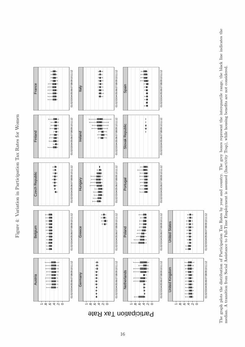
In order to identify β, we need tax-benefit reforms affecting the take-home wage differently

across demographic groups within a country. Recall that 1 − τi captures changes in income

tax regimes, but also in benefit generosity and market incomes. The variation of PTR

across years and countries is presented in Figures 4 and 5 across years and countries.

Countries like Hungary and Ireland exhibit substantial variation in work incentives, while

identification of β might be rather problematic for Germany. With the sample mean tax

rate and employment rate, the extensive elasticity can then be calculated by using the

definition of the extensive elasticity (Immervoll et al., 2007): εext = β (1−τ)E

.6

Country-wise estimates can be obtained by allowing the coefficient for 1 − τ to vary

across countries.

Ei = α + β (1 − τi) + γc (1 − τi) × cc + αg + µt + cc + ηi (4)

In this case, the country-specific elasticity is given by εext = (β + γc)(1−τ)E

.

A further focus of this study is to investigate to what extent workers’ responsiveness

to tax incentives β vary with economic and institutional circumstances. As an example,

workers might react less to lower PTRs in times of recessions due to demand-side con-

straints. The presence of active labor market policies (ALMP) might also dampen workers’

responsiveness, because participation in a training program might conflict with applying

6Equation 3 can also be estimated by GLS using the group-specific means for employment and taxrates, weighted by the number of observations in each cell.(Blundell et al. (1998a) and Angrist and Pischke(2009, p. 136))

4

for a job. To our knowledge, we are the first to investigate this kind of relationships with

a micro-estimated behavioral parameter. There are however studies that systematically

investigate the impact of policies and institutions on the level of (un)employment on the

national level.(Bassanini and Duval, 2006; Nickell, 1997)

In order to capture the influence of such confounders, the econometric model is en-

hanced by interacting the net PTR with a country-specific institutional indicator.

Ei = α + β(1 − τi) + δ(1 − τi) × Z∗ct + θZ∗

ct + αg + µt + εi (5)

In order to maintain the interpretation of β as the responsiveness at the mean, the indi-

cator is normalized by its country mean: Z∗ct = Zct − Zc. In particular, we apply GDP

growth, the Output gap and the ratio of unemployed persons to vacancies (UV Ratio) as

measures for the business cycle. Beyond, we consider ALMP spending and the level of

the minimum wage.

4 Results

We start by providing visual evidence on the bivariate relationship between Employment

and work incentives at the extensive margin. Figure 1 contrasts average Employment

rates with the respective mean PTR. For ease of interpretation, we use the net of PTR,

i. e. the change in net income, in what follows. Moreover, we consider the transition from

receiving basic social assistance to Full-Time Employment (Inactivity Trap). Apart from

demonstrating an overall lower employment rate of women, Figure 1 suggests a negative

relationship between Employment and potential earnings for women.7

To demonstrate the idea behind our empirical approach, Figure 2 shows the same

relationship for the US, broken down by skill groups. Each dot represents one demographic

group in one year. As can be seen, the overall negative slope is driven by differences

across skill groups, which might be an indication for different tastes for work across skill

groups. The estimation approach we apply controls for these group-specific unobserved

characteristics, and exploit divergent

7See also Kleven (2014).

5

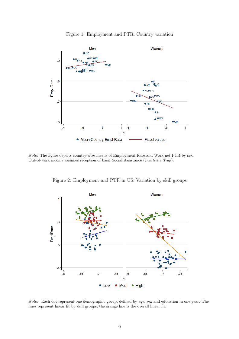
Figure 1: Employment and PTR: Country variation

Note: The figure depicts country-wise means of Employment Rate and Work net PTR by sex.Out-of-work income assumes reception of basic Social Assistance (Inactivity Trap).

Figure 2: Employment and PTR in US: Variation by skill groups

Note: Each dot represent one demographic group, defined by age, sex and education in one year. Thelines represent linear fit by skill groups, the orange line is the overall linear fit.

6

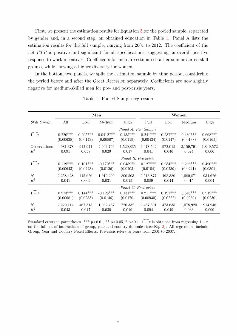
First, we present the estimation results for Equation 3 for the pooled sample, separated

by gender and, in a second step, on obtained education in Table 1. Panel A lists the

estimation results for the full sample, ranging from 2001 to 2012. The coefficient of the

net PTR is positive and significant for all specifications, suggesting an overall positive

response to work incentives. Coefficients for men are estimated rather similar across skill

groups, while showing a higher diversity for women.

In the bottom two panels, we split the estimation sample by time period, considering

the period before and after the Great Recession separately. Coefficients are now slightly

negative for medium-skilled men for pre- and post-crisis years.

Table 1: Pooled Sample regression

Men Women

Skill Group: All Low Medium High Full Low Medium High

Panel A: Full Sample

1 − τ 0.220*** 0.205*** 0.0412*** 0.135*** 0.241*** 0.237*** 0.430*** 0.668***(0.00638) (0.0143) (0.00807) (0.0119) (0.00434) (0.0147) (0.0138) (0.0165)

Observations 4,981,378 912,941 2,044,766 1,520,835 4,478,542 972,015 2,159,791 1,849,572R2 0.091 0.057 0.029 0.017 0.041 0.046 0.024 0.006

Panel B: Pre-crisis

1 − τ 0.119*** 0.101*** -0.170*** 0.0459** 0.127*** 0.254*** 0.206*** 0.490***(0.00643) (0.0223) (0.0126) (0.0203) (0.0104) (0.0239) (0.0241) (0.0301)

N 2,258,428 445,626 1,012,299 800,503 2,513,877 498,380 1,080,871 934,626R2 0.041 0.069 0.031 0.015 0.089 0.044 0.015 0.004

Panel C: Post-crisis

1 − τ 0.273*** 0.144*** -0.125*** 0.131*** 0.211*** 0.197*** 0.546*** 0.912***(0.00681) (0.0233) (0.0146) (0.0170) (0.00930) (0.0222) (0.0239) (0.0230)

N 2,220,114 467,315 1,032,467 720,332 2,467,501 473,635 1,078,920 914,946R2 0.043 0.047 0.030 0.019 0.094 0.049 0.033 0.009

Standard errors in parentheses. *** p<0.01, ** p<0.05, * p<0.1. 1 − τ is obtained from regressing 1− τon the full set of interactions of group, year and country dummies (see Eq. 3). All regressions includeGroup, Year and Country Fixed Effects. Pre-crisis refers to years from 2001 to 2007.

7

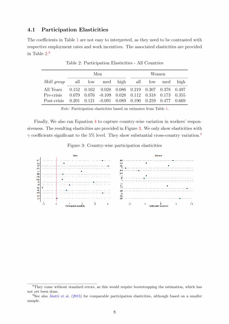
4.1 Participation Elasticities

The coefficients in Table 1 are not easy to interpreted, as they need to be contrasted with

respective employment rates and work incentives. The associated elasticities are provided

in Table 2.8

Table 2: Participation Elasticities - All Countries

Men Women

Skill group all low med high all low med high

All Years 0.152 0.162 0.028 0.086 0.219 0.307 0.378 0.497Pre-crisis 0.079 0.076 -0.109 0.028 0.112 0.318 0.173 0.355Post-crisis 0.201 0.121 -0.091 0.089 0.190 0.259 0.477 0.669

Note: Participation elasticities based on estimates from Table 1.

Finally, We also ran Equation 4 to capture country-wise variation in workers’ respon-

siveness. The resulting elasticities are provided in Figure 3. We only show elasticities with

γ coefficients significant to the 5% level. They show substantial cross-country variation.9

Figure 3: Country-wise participation elasticities

8They come without standard errors, as this would require bootstrapping the estimation, which hasnot yet been done.

9See also Jantti et al. (2015) for comparable participation elasticities, although based on a smallersample.

8

4.2 When are workers (not) responsive?

The main contribution of this paper is to go beyond ’traditional’ micro-based estimates

on labor supply, but to provide an analysis of interactions of individual labor supply

with economic and institutional confounders. The results for this interaction term δ

from equation 5 are provided in Table 3. We apply one time-demeaned variable Z∗ct at

once. Hence, every estimate from Table 3 represents a distinct regression with a full

set of country, year and group dummies. The coefficients can be interpreted as added

components It should be noted that data on vacancies and ALMP spending are not

available for all years and countries. Similarly, only a subset of countries have imposed

a statutory minimum wage. As a consequence, the underlying samples are not identical

across specifications.

The first two rows are to capture workers’ responsiveness across the business cycle.

Coefficients are significant throughout, but small in magnitude.10 Interestingly though, all

three business cycle indicators affect labor supply responses by men and women differently.

While women tend to slightly more reactive in times of recessions, the opposite holds for

men.

Next we consider the tightness of the labor market, defined as the ratio between

unemployed workers and job vacancies. The comparability of this measure across countries

is limited due to different definitions and accuracy of vacancy statistics.11 There is however

only a limited effect on labor supply responses, irrespective of sex.12

An interesting institution that may impact exits from inactivity or unemployment is

the prevalence of labor market policies. A plausible hypothesis is that tax-benefit reforms

have lower employment impacts if relatively many unemployed are participating in e. g.

training programmes. Counter to this hypothesis, there is some evidence that men are

more responsive if a government spends more on Active Labor Market Policies. This

measure however takes values in a narrow range between -.32 and .25, suggesting that

increasing ALMP spending per unemployed by a tenth of GDP per capita would raise the

coefficient for men by about 0.017. While the coefficient for women is negative, it even

smaller.

Finally, it is regularly stated that a high minimum wage has adverse effects on em-

ployment by raising labor costs. On the other hand, it guarantees a certain minimum

income if workers find a job. If reservation wages are high, a higher statutory minimum

wage might incentivize job-seekers. Our estimations support rather the latter view. The

apparently high coefficient has however to be set in perspective, as it is identified from a

minimum wage ratio ranging between 34 and 62% of median wage. Raising the minimum

10The normalized Output gap takes values between -8.5 and 7, the majority of countries moving in abandwidth of about 5.

11 While vacancy statistics for Austria cover the whole country, Finnish and German numbers reflectonly those vacancies that are reported to the employment agencies. (OECD, 2014a).

12The normalized UV ratio takes values between -30 and 56.

9

Table 3: Estimates for economic and institutional confounders

Men Women

Output Gap -0.011*** 0.016***(0.001) (0.001)

GDP Growth rate -0.009*** 0.013***(0.001) (0.001)

UV Ratio 0.001*** -0.002***(0.000) (0.000)

ALMP Spending per unemployed 0.169*** -0.047**(0.020) (0.023)

Minimum Wage / Median Wage 1.772*** 0.531***(0.097) (0.121)

The table shows estimates for δ in Equation 5 with full set of country, group and yeardummies. Standard errors in parentheses. *** p<0.01, ** p<0.05, * p<0.1. All variablescome from the OECD data base and are normalized by their country mean. ALMP Spendingper unemployed is divided by GDP per capita in order to net out country wealth. Theminimum wage level is defined by the statutory minimum wage, divided by the medianwage for a full-time worker.

wage by a tenth relative to the median wage would hence increase the baseline coefficient

by around 0.17 for men and 0.05 for women.

5 Conclusion

This paper provides micro-estimates on extensive labor supply elasticities for 20 OECD

countries. We contribute to the existing literature by relying on comprehensive data cov-

ering up to 12 years, totaling to around 8 million individual observations. While this time

span is long enough to capture tax-benefit changes, including reforms after the Great

Recession, the assumption of constant behavioral parameters is still justified. These em-

ployment data are combined with the OECD tax-benefit calculator, thereby obtaining

comprehensive work incentive measures. Our estimation approach exploits variation in

employment rates between demographic groups. Our results for the extensive labor supply

elasticity are almost uniformly non-negative, which is line with previous findings. At the

same time, there is substantial degree of heterogeneity between countries. On a second

step, we interact the participation tax rate with country-specific economic and institu-

tional factors. Our preliminary results indicate heterogeneous interactions between men

and women with regard to the business cycle and the prevalence of Active Labor Mar-

ket Policies. This suggests that tax-benefit reforms aiming at increasing work incentives

indeed work differently in different circumstances. The above findings are admittedly

rather reduced-form. Further steps in this analysis would include time lags or several

confounders at once to capture interdependencies.

Extensions of the present work will explore the reasons for different estimates before

10

and after the Great Recession. It seems also promising to investigate the sensitivity of

our results with respect to other PTR definitions.

11

References

Angrist, J. D. and Pischke, J.-S. (2009). Mostly Harmless Econometrics, Princeton Uni-

versity Press.

Bargain, O., Orsini, K. and Peichl, A. (2014). Comparing Labor Supply Elasticities in

Europe and the US: New Results, Journal of Human Resources 49(3): 723–838.

Bassanini, A. and Duval, R. (2006). Employment Patterns in OECD Countries: Re-

assessing the role of policies and institutions, OECD Social, Employment and Migration

Working Paper No. 35.

Blau, F. D. and Kahn, L. M. (2007). Changes in the labor supply behavior of married

women: 1980–2000, Journal of Labor Economics 25(3).

Blundell, R., Duncan, A. and Meghir, C. (1998a). Estimating labor supply responses

using tax reforms, Econometrica pp. 827–861.

Blundell, R., Duncan, A. and Meghir, C. (1998b). Estimating Labour Supply Responses

Using Tax Reforms, Econometrica 66(4)(4): 827–861.

Carone, G., Immervoll, H., Paturot, D. and Salomaki, A. (2004). Indicators of Unem-

ployment and Low-Wage Traps: Marginal Effective Tax Rates on Employment Incomes,

OECD Social, Employment and Migration Working Papers 18, OECD Publishing.

Chetty, R. (2012). Bounds on Elasticities With Optimization Frictions: A Synthesis of

Micro and Macro Evidence on Labor Supply, Econometrica 80(3): 969–1018.

Chetty, R., Guren, A., Manoli, D. and Weber, A. (2011). Are micro and macro labor

supply elasticities consistent? a review of evidence on the intensive and extensive

margins, American Economic Review 101(3): 471–75.

Heim, B. T. (2007). The incredible shrinking elasticities – married female labor supply,

1978–2002, Journal of Human Resources 42(4): 881–918.

Immervoll, H., Kleven, H. J., Kreiner, C. T. and Saez, E. (2007). Welfare reform in

european countries: a microsimulation analysis, The Economic Journal 117(516): 1–

44.

Jantti, M., Pirttila, J. and Selin, H. (2015). Estimating labour supply elasticities based

on cross-country micro data: A bridge between micro and macro estimates?, Journal

of Public Economics, forthcoming 127: 87–99.

Keane, M. P. (2011). Labor supply and taxes: A survey, Journal of Economic Literature

49(4): 961 – 1075.

12

Kleven, H. J. (2014). How Can Scandinavians Tax So Much?, Journal of Economic

Perspectives 28(4): 77–98.

Nickell, S. (1997). Unemployment and labour market rigidities: Europe versus North

America, Journal of Economic Perspectives 11(3): 55–74.

OECD (2014a). An Update on the Labour Market Situation – Further Material. Annex

of Chapter 1 of the OECD Employment Outlook 2014 OECD Publishing, Paris,.

OECD (2014b). Education at a Glance 2014: OECD Indicators. OECD Publishing.

Pestel, N. and Bartels, C. (2015). The Impact of Short- and Long-term Participation Tax

Rates on Labor Supply. IZA Discussion Paper No. 9151.

Prescott, E. C. (2004). Why do americans work so much more than europeans?, Technical

report, National Bureau of Economic Research.

Saez, E. (2001). Using elasticities to derive optimal income tax rates, Review of Economic

Studies 68(1): 205–229.

13

Tab

le4:

Sam

ple

Siz

eby

Cou

ntr

yan

dY

ear

2001

2002

2003

2004

2005

2006

2007

2008

2009

2010

2011

2012

AT

10,7

1848,7

34

47,6

51

48,1

29

45,0

74

43,4

58

43,0

82

42,5

71

42,2

15

BE

6,66

37,

555

7,31

88,

018

30,8

72

31,6

12

30,7

45

28,3

90

27,5

99

26,9

83

24,6

87

24,0

57

CZ

15,1

8259,6

52

60,1

23

58,5

67

55,2

29

52,1

50

51,7

63

9,9

42

9,6

62

DE

88,8

7487

,855

87,8

9285

,756

132,4

04

13,9

62

13,7

79

13,1

99

13,6

33

12,9

47

12,9

40

129,9

00

ES

35,6

4535

,550

35,7

5736

,445

125,9

35

21,9

08

21,8

80

22,7

68

23,5

54

23,9

93

23,6

54

24,2

14

FI

17,6

9616

,933

16,3

53

15,9

08

15,1

74

15,3

62

14,7

77

14,3

34

13,4

59

13,3

34

FR

22,7

3522

,431

84,5

38

82,1

45

83,0

78

80,9

55

95,8

84

112,3

91

116,4

71

114,3

38

GR

70,9

43

72,9

65

64,0

31

54,5

18

HU

17,7

4816

,577

18,2

4116

,891

61,1

41

60,1

13

58,7

09

53,3

34

51,8

41

49,1

19

48,2

36

45,4

21

IE19,3

90

18,8

11

16,9

30

66,0

06

60,3

57

56,0

53

57,4

93

IT39

,004

159,7

74

155,3

66

153,9

80

153,8

13

150,9

84

151,1

60

146,9

32

133,0

30

NL

32,3

8334

,389

33,6

6438

,904

158,5

87

35,2

68

34,0

77

34,3

70

28,6

67

25,1

74

26,3

92

24,3

71

PL

11,9

5112

,001

45,9

36

43,9

57

41,3

65

40,7

40

42,2

99

81,0

95

81,0

04

79,5

73

PT

11,1

3541,3

35

38,0

30

35,0

55

34,1

04

33,6

62

32,9

10

29,0

42

28,1

98

SK

18,9

64

18,1

60

17,7

29

17,5

86

16,9

63

UK

32,1

0531

,582

29,8

2631

,664

30,7

98

29,8

24

29,3

90

46,3

17

22,3

74

21,3

59

20,6

83

19,7

91

US

199,

791

218,

253

213,

115

208,

009

204,5

33

200,5

42

196,9

19

194,3

91

192,1

93

184,9

36

177,2

31

175,1

93

14

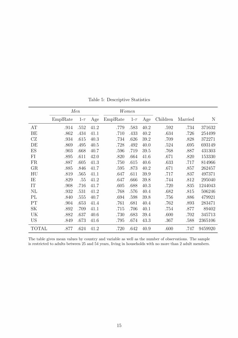
Table 5: Descriptive Statistics

Men Women

EmplRate 1-τ Age EmplRate 1-τ Age Children Married N

AT .914 .552 41.2 .779 .583 40.2 .592 .734 371632BE .862 .434 41.1 .710 .433 40.2 .634 .726 254499CZ .934 .615 40.3 .734 .626 39.2 .709 .828 372271DE .869 .495 40.5 .728 .492 40.0 .524 .695 693149ES .903 .668 40.7 .596 .719 39.5 .768 .887 431303FI .895 .611 42.0 .820 .664 41.6 .671 .820 153330FR .887 .605 41.3 .750 .615 40.6 .633 .717 814966GR .885 .846 41.7 .595 .873 40.2 .671 .857 262457HU .819 .565 41.1 .647 .611 39.9 .717 .837 497371IE .829 .55 41.2 .647 .666 39.8 .744 .812 295040IT .908 .716 41.7 .605 .688 40.3 .720 .835 1244043NL .932 .531 41.2 .768 .576 40.4 .682 .815 506246PL .840 .555 40.7 .694 .598 39.8 .756 .886 479921PT .904 .653 41.4 .761 .681 40.4 .762 .893 283471SK .892 .709 41.1 .715 .706 40.1 .754 .877 89402UK .882 .637 40.6 .730 .683 39.4 .600 .702 345713US .849 .673 41.6 .795 .674 43.3 .367 .588 2365106

TOTAL .877 .624 41.2 .720 .642 40.9 .600 .747 9459920

The table gives mean values by country and variable as well as the number of observations. The sampleis restricted to adults between 25 and 54 years, living in households with no more than 2 adult members.

15

Fig

ure

4:V

aria

tion

inP

arti

cipat

ion

Tax

Rat

esfo

rW

omen

0.2.4.6.81 0.2.4.6.81 0.2.4.6.81 0.2.4.6.81

0102

0304

0506

0708

0910

1112

0102

0304

0506

0708

0910

1112

0102

0304

0506

0708

0910

1112

0102

0304

0506

0708

0910

1112

0102

0304

0506

0708

0910

1112

0102

0304

0506

0708

0910

1112

0102

0304

0506

0708

0910

1112

0102

0304

0506

0708

0910

1112

0102

0304

0506

0708

0910

1112

0102

0304

0506

0708

0910

1112

0102

0304

0506

0708

0910

1112

0102

0304

0506

0708

0910

1112

0102

0304

0506

0708

0910

1112

0102

0304

0506

0708

0910

1112

0102

0304

0506

0708

0910

1112

0102

0304

0506

0708

0910

1112

0102

0304

0506

0708

0910

1112

Aus

tria

Bel

gium

Cze

ch R

epub

licF

inla

ndF

ranc

e

Ger

man

yG

reec

eH

unga

ryIr

elan

dIta

ly

Net

herla

nds

Pol

and

Por

tuga

lS

lova

k R

epub

licS

pain

Uni

ted

Kin

gdom

Uni

ted

Sta

tes

Participation Tax Rate

Th

egr

aph

plo

tsth

ed

istr

ibu

tion

ofP

arti

cip

atio

nT

axR

ates

by

year

an

dco

untr

y.T

he

gre

yb

oxes

rep

rese

nt

the

inte

rqu

art

ile

ran

ge,

the

bla

ckli

ne

ind

icate

sth

em

edia

n.

Atr

ansi

tion

from

Soci

alA

ssis

tan

ceto

Fu

ll-T

ime

Em

plo

ym

ent

isass

um

ed(I

nact

ivit

yT

rap

),w

hil

eh

ou

sin

gb

enefi

tsare

not

con

sid

ered

.

16

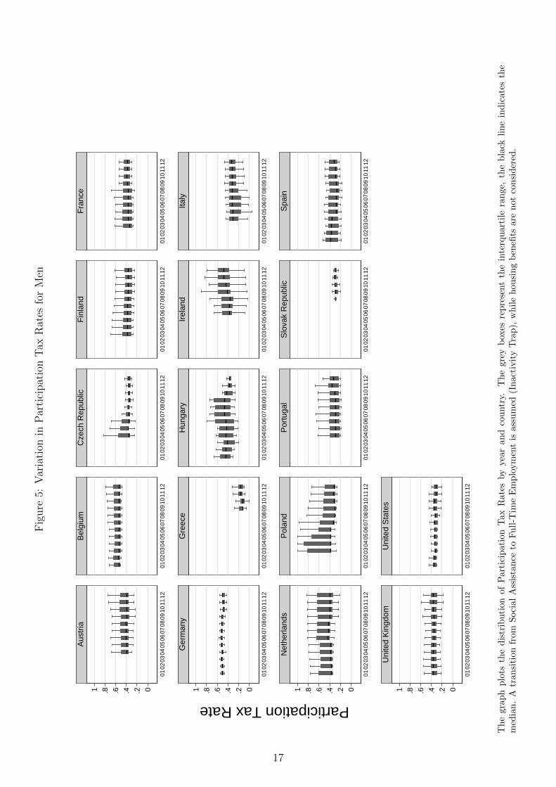
Fig

ure

5:V

aria

tion

inP

arti

cipat

ion

Tax

Rat

esfo

rM

en

0.2.4.6.81 0.2.4.6.81 0.2.4.6.81 0.2.4.6.81

0102

0304

0506

0708

0910

1112

0102

0304

0506

0708

0910

1112

0102

0304

0506

0708

0910

1112

0102

0304

0506

0708

0910

1112

0102

0304

0506

0708

0910

1112

0102

0304

0506

0708

0910

1112

0102

0304

0506

0708

0910

1112

0102

0304

0506

0708

0910

1112

0102

0304

0506

0708

0910

1112

0102

0304

0506

0708

0910

1112

0102

0304

0506

0708

0910

1112

0102

0304

0506

0708

0910

1112

0102

0304

0506

0708

0910

1112

0102

0304

0506

0708

0910

1112

0102

0304

0506

0708

0910

1112

0102

0304

0506

0708

0910

1112

0102

0304

0506

0708

0910

1112

Aus

tria

Bel

gium

Cze

ch R

epub

licF

inla

ndF

ranc

e

Ger

man

yG

reec

eH

unga

ryIr

elan

dIta

ly

Net

herla

nds

Pol

and

Por

tuga

lS

lova

k R

epub

licS

pain

Uni

ted

Kin

gdom

Uni

ted

Sta

tes

Participation Tax Rate

Th

egr

aph

plo

tsth

ed

istr

ibu

tion

ofP

arti

cip

atio

nT

axR

ates

by

year

an

dco

untr

y.T

he

gre

yb

oxes

rep

rese

nt

the

inte

rqu

art

ile

ran

ge,

the

bla

ckli

ne

ind

icate

sth

em

edia

n.

Atr

ansi

tion

from

Soci

alA

ssis

tan

ceto

Fu

ll-T

ime

Em

plo

ym

ent

isass

um

ed(I

nact

ivit

yT

rap

),w

hil

eh

ou

sin

gb

enefi

tsare

not

con

sid

ered

.

17