Michael Ulbrich Nonsmooth Newton-like Methods for ... · Michael Ulbrich Nonsmooth Newton-like...
208
Michael Ulbrich Nonsmooth Newton-like Methods for Variational Inequalities and Constrained Optimization Problems in Function Spaces Technische Universit¨ at M¨ unchen Fakult¨ at f ¨ ur Mathematik June 2001, revised February 2002
Transcript of Michael Ulbrich Nonsmooth Newton-like Methods for ... · Michael Ulbrich Nonsmooth Newton-like...

MichaelUlbrich
NonsmoothNewton-likeMethods forVariational Inequalities and Constrained
Optimization Problemsin Function Spaces
TechnischeUniversitatMunchen
Fakultat fur Mathematik
June2001,revisedFebruary2002

Table of Contents
1. Intr oduction . . . . . . . . . . . . . . . . . . . . . . . . . . . . . . . . . . . . . . . . . . . . . . . . 11.1 Examplesof Applications. . . . . . . . . . . . . . . . . . . . . . . . . . . . . . . . . . . . 4
1.1.1 OptimalControlProblems. . . . . . . . . . . . . . . . . . . . . . . . . . . . . 41.1.2 VariationalInequalities . . . . . . . . . . . . . . . . . . . . . . . . . . . . . . . 7
1.2 Motivationof theMethod. . . . . . . . . . . . . . . . . . . . . . . . . . . . . . . . . . . . 81.2.1 Finite-DimensionalVariationalInequalities . . . . . . . . . . . . . . 91.2.2 Infinite-DimensionalVariationalInequalities. . . . . . . . . . . . . 13
1.3 Organization . . . . . . . . . . . . . . . . . . . . . . . . . . . . . . . . . . . . . . . . . . . . . . 14
2. Elementsof Finite-DimensionalNonsmoothAnalysis. . . . . . . . . . . . . . 172.1 GeneralizedDifferentials. . . . . . . . . . . . . . . . . . . . . . . . . . . . . . . . . . . . 172.2 Semismoothness. . . . . . . . . . . . . . . . . . . . . . . . . . . . . . . . . . . . . . . . . . . 182.3 SemismoothNewton’sMethod . . . . . . . . . . . . . . . . . . . . . . . . . . . . . . . 202.4 HigherOrderSemismoothness. . . . . . . . . . . . . . . . . . . . . . . . . . . . . . . 222.5 Examplesof SemismoothFunctions. . . . . . . . . . . . . . . . . . . . . . . . . . . 23
2.5.1 TheEuclideanNorm . . . . . . . . . . . . . . . . . . . . . . . . . . . . . . . . . 232.5.2 TheFischer–BurmeisterFunction . . . . . . . . . . . . . . . . . . . . . . 242.5.3 PiecewiseDifferentiableFunctions . . . . . . . . . . . . . . . . . . . . . 24
2.6 Extensions. . . . . . . . . . . . . . . . . . . . . . . . . . . . . . . . . . . . . . . . . . . . . . . . 27
3. NewtonMethods for SemismoothOperator Equations . . . . . . . . . . . . 293.1 Introduction. . . . . . . . . . . . . . . . . . . . . . . . . . . . . . . . . . . . . . . . . . . . . . . 293.2 NewtonMethodsfor AbstractSemismoothOperators. . . . . . . . . . . . 34
3.2.1 SemismoothOperatorsin BanachSpaces. . . . . . . . . . . . . . . . 343.2.2 BasicProperties. . . . . . . . . . . . . . . . . . . . . . . . . . . . . . . . . . . . . 343.2.3 SemismoothNewton’sMethod. . . . . . . . . . . . . . . . . . . . . . . . . 373.2.4 InexactNewton’sMethod . . . . . . . . . . . . . . . . . . . . . . . . . . . . . 393.2.5 ProjectedInexactNewton’sMethod. . . . . . . . . . . . . . . . . . . . . 413.2.6 AlternativeRegularityConditions . . . . . . . . . . . . . . . . . . . . . . 42
3.3 SemismoothNewtonMethodsfor SuperpositionOperators. . . . . . . . 443.3.1 Assumptions. . . . . . . . . . . . . . . . . . . . . . . . . . . . . . . . . . . . . . . . 443.3.2 A GeneralizedDifferential . . . . . . . . . . . . . . . . . . . . . . . . . . . . 473.3.3 Semismoothnessof SuperpositionOperators. . . . . . . . . . . . . 493.3.4 Illustrations. . . . . . . . . . . . . . . . . . . . . . . . . . . . . . . . . . . . . . . . . 52

II Tableof Contents
3.3.5 Proofof theMain Theorems. . . . . . . . . . . . . . . . . . . . . . . . . . . 553.3.6 SemismoothNewtonMethods . . . . . . . . . . . . . . . . . . . . . . . . . 603.3.7 SemismoothCompositeOperatorsandChainRules . . . . . . . 643.3.8 FurtherPropertiesof theGeneralizedDifferential . . . . . . . . . 66
4. SmoothingStepsand Regularity Conditions . . . . . . . . . . . . . . . . . . . . . 694.1 SmoothingSteps. . . . . . . . . . . . . . . . . . . . . . . . . . . . . . . . . . . . . . . . . . . 694.2 A NewtonMethodwithoutSmoothingSteps. . . . . . . . . . . . . . . . . . . . 704.3 SufficientConditionsfor Regularity . . . . . . . . . . . . . . . . . . . . . . . . . . . 72
5. Variational Inequalities and Mixed Problems . . . . . . . . . . . . . . . . . . . . 795.1 Applicationto VariationalInequalities. . . . . . . . . . . . . . . . . . . . . . . . . 79
5.1.1 Problemswith Bound-Constraints. . . . . . . . . . . . . . . . . . . . . . 795.1.2 PointwiseConvex Constraints. . . . . . . . . . . . . . . . . . . . . . . . . . 83
5.2 MixedProblems. . . . . . . . . . . . . . . . . . . . . . . . . . . . . . . . . . . . . . . . . . . 885.2.1 Karush–Kuhn–TuckerSystems. . . . . . . . . . . . . . . . . . . . . . . . . 895.2.2 Connectionsto theReducedProblem. . . . . . . . . . . . . . . . . . . . 935.2.3 RelationsbetweenFull andReducedNewtonSystem. . . . . . 955.2.4 SmoothingSteps. . . . . . . . . . . . . . . . . . . . . . . . . . . . . . . . . . . . . 985.2.5 RegularityConditions . . . . . . . . . . . . . . . . . . . . . . . . . . . . . . . . 99
6. Trust-RegionGlobalization . . . . . . . . . . . . . . . . . . . . . . . . . . . . . . . . . . . 1016.1 TheTrust-RegionAlgorithm . . . . . . . . . . . . . . . . . . . . . . . . . . . . . . . . . 1056.2 GlobalConvergence. . . . . . . . . . . . . . . . . . . . . . . . . . . . . . . . . . . . . . . . 1086.3 ImplementableDecreaseConditions. . . . . . . . . . . . . . . . . . . . . . . . . . . 1146.4 Transitionto FastLocalConvergence. . . . . . . . . . . . . . . . . . . . . . . . . . 116
7. Applications . . . . . . . . . . . . . . . . . . . . . . . . . . . . . . . . . . . . . . . . . . . . . . . . 1217.1 DistributedControlof aNonlinearElliptic Equation . . . . . . . . . . . . . 121
7.1.1 Black-BoxApproach. . . . . . . . . . . . . . . . . . . . . . . . . . . . . . . . . 1247.1.2 All-at-OnceApproach. . . . . . . . . . . . . . . . . . . . . . . . . . . . . . . . 1287.1.3 FiniteElementDiscretization. . . . . . . . . . . . . . . . . . . . . . . . . . 1297.1.4 DiscreteBlack-Box-Approach. . . . . . . . . . . . . . . . . . . . . . . . . 1327.1.5 EfficientSolutionof theNewtonSystem. . . . . . . . . . . . . . . . . 1387.1.6 DiscreteAll-at-OnceApproach . . . . . . . . . . . . . . . . . . . . . . . . 142
7.2 NumericalResults. . . . . . . . . . . . . . . . . . . . . . . . . . . . . . . . . . . . . . . . . . 1427.2.1 UsingMultigrid Techniques. . . . . . . . . . . . . . . . . . . . . . . . . . . 1437.2.2 Black-BoxApproach. . . . . . . . . . . . . . . . . . . . . . . . . . . . . . . . . 1457.2.3 All-at-OnceApproach. . . . . . . . . . . . . . . . . . . . . . . . . . . . . . . . 1487.2.4 NestedIteration . . . . . . . . . . . . . . . . . . . . . . . . . . . . . . . . . . . . . 1507.2.5 Discussionof theResults. . . . . . . . . . . . . . . . . . . . . . . . . . . . . . 151
7.3 ObstacleProblems. . . . . . . . . . . . . . . . . . . . . . . . . . . . . . . . . . . . . . . . . . 1527.3.1 DualProblem. . . . . . . . . . . . . . . . . . . . . . . . . . . . . . . . . . . . . . . 1537.3.2 RegularizedDual Problem . . . . . . . . . . . . . . . . . . . . . . . . . . . . 1557.3.3 Discretization. . . . . . . . . . . . . . . . . . . . . . . . . . . . . . . . . . . . . . . 158

Tableof Contents III
7.3.4 NumericalResults . . . . . . . . . . . . . . . . . . . . . . . . . . . . . . . . . . . 160
8. Optimal Control of the IncompressibleNavier–StokesEquations. . . . 1678.1 Introduction. . . . . . . . . . . . . . . . . . . . . . . . . . . . . . . . . . . . . . . . . . . . . . . 1678.2 FunctionalAnalytic Settingof theControlProblem. . . . . . . . . . . . . . 168
8.2.1 FunctionSpaces. . . . . . . . . . . . . . . . . . . . . . . . . . . . . . . . . . . . . 1688.2.2 TheControlProblem. . . . . . . . . . . . . . . . . . . . . . . . . . . . . . . . . 169
8.3 Analysisof theControlProblem. . . . . . . . . . . . . . . . . . . . . . . . . . . . . . 1718.3.1 StateEquation. . . . . . . . . . . . . . . . . . . . . . . . . . . . . . . . . . . . . . . 1718.3.2 Control-to-StateMapping . . . . . . . . . . . . . . . . . . . . . . . . . . . . . 1758.3.3 Adjoint Equation . . . . . . . . . . . . . . . . . . . . . . . . . . . . . . . . . . . . 1768.3.4 Propertiesof theReducedObjectiveFunction . . . . . . . . . . . . 179
8.4 Applicationof SemismoothNewtonMethods. . . . . . . . . . . . . . . . . . . 181
9. Optimal Control of the CompressibleNavier–StokesEquations . . . . . 1839.1 Introduction. . . . . . . . . . . . . . . . . . . . . . . . . . . . . . . . . . . . . . . . . . . . . . . 1839.2 TheFlow ControlProblem. . . . . . . . . . . . . . . . . . . . . . . . . . . . . . . . . . . 1839.3 Adjoint-BasedGradientComputation. . . . . . . . . . . . . . . . . . . . . . . . . . 1859.4 SemismoothBFGS-NewtonMethod. . . . . . . . . . . . . . . . . . . . . . . . . . . 186
9.4.1 Quasi-NewtonBFGS-Approximations. . . . . . . . . . . . . . . . . . 1869.4.2 TheAlgorithm . . . . . . . . . . . . . . . . . . . . . . . . . . . . . . . . . . . . . . 187
9.5 NumericalResults. . . . . . . . . . . . . . . . . . . . . . . . . . . . . . . . . . . . . . . . . . 188
A. Appendix . . . . . . . . . . . . . . . . . . . . . . . . . . . . . . . . . . . . . . . . . . . . . . . . . . 191A.1 Adjoint Approachfor OptimalControlProblems. . . . . . . . . . . . . . . . 191
A.1.1 Adjoint Representationof theReducedGradient. . . . . . . . . . 191A.1.2 Adjoint Representationof theReducedHessian. . . . . . . . . . . 192
A.2 SeveralInequalities. . . . . . . . . . . . . . . . . . . . . . . . . . . . . . . . . . . . . . . . . 194A.3 ElementaryPropertiesof Multifunctions . . . . . . . . . . . . . . . . . . . . . . . 194A.4 NemytskijOperators. . . . . . . . . . . . . . . . . . . . . . . . . . . . . . . . . . . . . . . . 195
Notations . . . . . . . . . . . . . . . . . . . . . . . . . . . . . . . . . . . . . . . . . . . . . . . . . . . . . . 199
References. . . . . . . . . . . . . . . . . . . . . . . . . . . . . . . . . . . . . . . . . . . . . . . . . . . . . 201

Acknowledgments
It is my greatpleasureto thankProf. Dr. KlausRitter for his constantsupportandencouragementover thepasttenyears.Furthermore,I would like to thankProf.Dr.JohannEdenhoferwhostimulatedmy interestin optimalcontrolof PDEs.
My scientific work benefitedsignificantly from two very enjoyable and fruit-ful researchstaysat the Departmentof Computationaland Applied Mathematics(CAAM) andtheCenterfor Researchon ParallelComputation(CRPC),RiceUni-versity, Houston,Texas.Thesevisits weremadepossibleby Prof. JohnDennisandProf. MatthiasHeinkenschloss.I am very thankful to bothof themfor their hospi-tality andsupport.During my secondstayat Rice University, I laid the foundationof a large part of this work. The visits were fundedby the ForschungsstipendiumUl157/1-1andtheHabilitandenstipendiumUl157/3-1of theDeutscheForschungs-gemeinschaft,and by CRPC grant CCR-9120008.This supportis gratefully ac-knowledged.
The computationalresultsin chapter9 for the boundarycontrol of the com-pressibleNavier–Stokesequationsbuild on joint work with Prof.ScottCollis, Prof.MatthiasHeinkenschloss,Dr. KavehGhayour, andDr. StefanUlbrich aspartof theRice AeroAcousticControl (RAAC) project,which is directedby ScottCollis andMatthiasHeinkenschloss.I thankall RAAC groupmembersfor allowing meto usetheir contributions to the project for my computations.In particular, ScottCollis’Navier–Stokessolver wasvery helpful. The computationsfor chapter9 wereper-formedonanSGIOrigin 2000atRiceUniversitywhichwaspurchasedwith theaidof NSF SCREMSgrant98–72009.I am very thankful to MatthiasHeinkenschlossfor giving me accessto this machine.Furthermore,I would like to thankProf. Dr.FolkmarBornemannfor theopportunityto usehisSGIOrigin 200for computations.
I also would like to acknowledgethe ZentrumMathematik,TechnischeUni-versitat Munchen,for providing a very pleasantandprofessionalworking environ-ment.In particular, I amthankfulto themembersof ourRechnerbetriebsgruppe,Dr.MichaelNast,Dr. AndreasJohann,andRolf Schone,for their goodsystemadmin-istrationandtheirhelpfulness.
In makingtheideasfor this work concrete,I profitedfrom an inspiringconver-sationwith Prof.Liqun Qi, Prof.Danny Ralph,andPDDr. ChristianKanzow duringtheICCP99meetingin Madison,Wisconsin,which I would like to acknowledge.
Finally, I wish to thankmy parents,MargotandPeter, andmy brotherStefanforalwaysbeingtherefor me.
1. Intr oduction
A centralthemeof appliedmathematicsis thedesignof accuratemathematicalmod-elsfor avarietyof technical,financial,medical,andmany otherapplications,andthedevelopmentof efficientnumericalalgorithmsfor theirsolution.Often,thesemodelscontainparametersthatshouldbeadjustedin anoptimalway, eitherto maximizetheaccuracy of themodel(parameteridentification),or to control thesimulatedsystemin a desiredway (optimal control).Sinceoptimizationwith simulationconstraintsis morechallengingthansimulationalone(which alreadycanbe very involved onits own), the developmentandanalysisof efficient optimizationmethodsis crucialfor theviability of thisapproach.Besidestheoptimizationof systems,minimizationproblemsandvariationalinequalitiesoften arisealreadyin the processof buildingmathematicalmodels;this, e.g.,appliesto contactproblems,free boundaryprob-lems,andelastoplasticproblems[47, 62,63,97,98,117].
Mostof thevariationalproblemsmentionedsofar join thepropertythatthey arecontinuousin timeand/orspace,sothatinfinite-dimensionalfunctionspacesprovidetheappropriatesettingfor theiranalysis.Sinceessentialinformationon theproblemto solveis carriedby thepropertiesof theunderlyinginfinite-dimensionalspaces,thesuccessfuldesignof robustandmesh-independentoptimizationmethodsrequiresathoroughconvergenceanalysisin this infinite-dimensionalfunction spacesetting.Thepurposeof this work is to developandanalyzea classof Newton-typemethodsfor thesolutionof optimizationproblemsandvariationalinequalitiesthatareposedin function spacesand containpointwiseinequality constraints. A representativeprototypeof theproblemsweconsiderhereis thefollowing:
Bound-ConstrainedVariational Inequality Problem(VIP):
Findu ∈ Lp(Ω) suchthat:
u ∈ B def= v ∈ Lp(Ω) : a ≤ v ≤ b on Ω,〈F (u), v − u〉 ≥ 0 for all v ∈ B.
(1.1)
Hereby, 〈u, v〉 =∫Ωu(ω)v(ω)dω, andF : Lp(Ω) → Lp
′(Ω) with p, p′ ∈ (1,∞],
1/p + 1/p′ ≤ 1, is an (in generalnonlinear)operator, whereLp(Ω) is the usualLebesguespaceon theboundedLebesguemeasurablesetΩ ⊂ Rn. We assumethatΩ haspositive Lebesguemeasure,so that0 < µ(Ω) < ∞. TheserequirementsonΩ areassumedthroughoutthis work. In casethis is needed(e.g.,for embeddings),but not explicitly stated,we assumethatΩ is nonempty, open,andboundedwith

2 1. Introduction
sufficiently smoothboundary∂Ω. The lower- andupperboundfunctionsa andbmay be presentonly on measurablepartsΩa andΩb of Ω, which is achieved bysettinga|Ω\Ωa
= −∞ andb|Ω\Ωb= +∞, respectively. We assumethatthenatural
extensionsby zeroof a|Ωaandb|Ωb
toΩ areelementsof Lp(Ω). We alsorequireaminimumdistanceν > 0 of theboundsfrom eachother, i.e.,b− a ≥ ν onΩ. In thedefinition of B, andthroughoutthis work, relationsbetweenmeasurablefunctionsaremeantto holdpointwisealmosteverywhereonΩ in theLebesguesense.Variousextensionsof problem(1.1)will alsobeconsideredandarediscussedbelow.
In many situations,the VIP (1.1) describesthe first-ordernecessaryoptimalityconditionsof thebound-constrainedminimizationproblem
minimize j(u) subjectto u ∈ B. (1.2)
In this case,F is the Frechetderivative j′ : Lp(Ω) → Lp(Ω)∗ of the objectivefunctionalj : Lp(Ω)→ R.
The methodswe aregoing to investigatearebestexplainedby consideringtheunilateralcasewith lower boundsa ≡ 0. Theresultingproblemis callednonlinearcomplementarityproblem(NCP):
u ∈ Lp(Ω), u ≥ 0, 〈F (u), v − u〉 ≥ 0 for all v ∈ Lp(Ω), v ≥ 0. (1.3)
As we will see,and as might be obvious to the reader, (1.3) is equivalent to thepointwisecomplementaritysystem
u ≥ 0, F (u) ≥ 0, uF (u) = 0 onΩ. (1.4)
The basicidea,which wasdevelopedin the ninetiesfor the numericalsolutionoffinite-dimensionalNCPs,consistsin the observation that (1.3) is equivalentto theoperatorequation
Φ(u) = 0, where Φ(u) = φ(u(ω), F (u)(ω)
)ω ∈ Ω. (1.5)
Hereby, φ : R2 → R is anNCP-function,i.e.,
φ(x) = 0 ⇐⇒ x1, x2 ≥ 0, x1x2 = 0.
Wewill developasemismoothnessconceptthatis applicableto theoperatorsarisingin (1.5)andthatallowsusto developaclassof Newton-typemethodsfor thesolutionof (1.5).Theresultingalgorithmshave,astheirfinite-dimensionalcounterparts– thesemismoothNewtonmethods– severalremarkableproperties:
(a) Themethodsarelocally superlinearlyconvergent,andthey convergewith q-rate> 1 underslightly strongerassumptions.
(b) Althoughaninequalityconstrainedproblemis solved,only onelinearoperatorequationhasto besolvedper iteration.Thus,thecostper iterationis compara-ble to thatof Newton’s methodfor smoothoperatorequations.We remarkthatsequentialquadraticprogramming(SQP)algorithms,whichareveryefficient in

1. Introduction 3
practice,requirethesolutionof aninequalityconstrainedquadraticprogramperiteration,which canbesignificantlymoreexpensive.Thus,it is alsoattractiveto combineSQPmethodswith theclassof Newton methodswe describehere,eitherby usingtheNewtonmethodfor solvingsubproblems,or by rewriting thecomplementarityconditionsin theKuhn–Tuckersystemasoperatorequation.
(c) Theconvergenceanalysisdoesnotrequireastrictcomplementarityconditiontohold. Therefore,we canprove fastconvergencealsofor thecasewherethesetω : u(ω) = 0, F (u)(ω) = 0 haspositivemeasureat thesolutionu.
(d) Thesystemsthathave to besolvedin eachiterationareof theform
[d1 · I + d2 · F ′(u)]s = −Φ(u), (1.6)
whereI : u 7→ u is the identity andF ′ denotesthe Frechetderivative of F .Further, d1, d2 arenonnegativeL∞-functionsthat arechosendependingon uandsatisfy0 < γ1 < d1 + d2 < γ2 on Ω uniformly in u. More precisely:(d1, d2) is ameasurableselectionof themeasurablemultifunction
ω ∈ Ω 7→ ∂φ(u(ω), F (u)(ω)
),
where∂φ is Clarke’sgeneralizedgradientof φ. As wewill see,in typicalappli-cationsthesystem(1.6)canbesymmetrizedandisnotmuchharderto solvethana systeminvolving only the operatorF ′(u), which would arisefor the uncon-strainedproblemF (u) = 0. In particular, fastsolverslike multigrid methods,preconditionediterative solvers,etc.,canbeappliedto solve(1.6).
(e) The methodis not restrictedto the problemclass(1.1). Among the possibleextensionswealsoinvestigatevariationalinequalityproblemsof theform (1.1),but with thefeasiblesetB replacedby
C = u ∈ Lp(Ω)m : u(ω) ∈ C on Ω, C ⊂ Rm closedandconvex.
Furthermore,we will considermixed problems,whereF (u) is replacedbyF (y, u) andwherewe have the additionaloperatorequationE(y, u) = 0. Inparticular, suchproblemsariseasthefirst-ordernecessaryoptimalityconditions(Karush–Kuhn–Tuckeror KKT-conditions)of optimizationproblemswith opti-mal controlstructure
minimize J(y, u) subjectto E(y, u) = 0, u ∈ C.
(f) Otherextensionsarepossiblethat we do not cover in this work. For instance,certain quasivariational inequalities[12, 13], i.e., variational inequalitiesforwhich thefeasiblesetdependsonu (e.g.,a = A(u), b = B(u)), canbesolvedby ourclassof semismoothNewtonmethods.
For illustration,webegin with examplesof two problemclassesthatfit in theaboveframework.

4 1. Introduction
1.1 Examplesof Applications
1.1.1 Optimal Control Problems
Let begiventhestatespaceY (aBanachspace),thecontrol spaceU = Lp(Ω), andthesetB ⊂ U of admissibleor feasiblecontrolsasdefinedin (1.1).Thestatey ∈ Yof thesystemunderconsiderationis governedby thestateequation
E(y, u) = 0, (1.7)
whereE : Y × U → W ∗ andW ∗ denotesthe dual of a reflexive BanachspaceW . In our context, the stateequationusually is given by the weakformulationofa partialdifferentialequation(PDE),includingall boundaryconditionsthatarenotalreadycontainedin the definition of Y . Supposethat, for every control u ∈ U ,the stateequation(1.7) possessesa uniquesolutiony = y(u) ∈ Y . The controlproblemconsistsin finding a control u suchthat the pair (y(u), u) minimizesagivenobjective functionJ : Y × U → R amongall feasiblecontrolsu ∈ B. Thus,thecontrolproblemis
minimizey∈Y,u∈U
J(y, u) subjectto (1.7) and u ∈ B. (1.8)
Alternatively, we canusethestateequationto expressthestatein termsof thecon-trol, y = y(u), andto write thecontrolproblemin theequivalentreducedform
minimize j(u) subjectto u ∈ B, (1.9)
with thereducedobjectivefunctionj(u) def= J(y(u), u). By theimplicit functionthe-orem,the continuousdifferentiability of y(u) in a neighborhoodof u follows if Eis continuouslydifferentiableandEy(y(u), u) is continuouslyinvertible.Further, ifin additionJ is continuouslydifferentiablein a neighborhoodof (y(u), u) thenj iscontinuouslydifferentiablein aneighborhoodof u. In thesameway, differentiabilityof higherordercanbeensured.For problem(1.9), thegradientj′(u) ∈ U∗ is givenby
j′(u) = Ju(y, u) + yu(u)∗Jy(y, u),
with y = y(u). Alternatively, j′ canberepresentedvia theadjointstatew = w(u) ∈W , which is thesolutionof theadjoint equation
Ey(y, u)∗w = −Jy(y, u),
wherey = y(u). As discussedin moredetail in appendixA.1, thegradientof j canbewritten in theform
j′(u) = Ju(y, u) + Eu(y, u)∗w.
Adjoint-basedexpressionsfor the secondderivative j′′ arealsoavailable,seeap-pendixA.1.

1.1 Examplesof Applications 5
We now make the examplemore concreteand consideras stateequationthePoissonproblemwith distributedcontrolon theright handside,
−∆y = u on Ω, y = 0 on ∂Ω, (1.10)
andanobjective functionof trackingtype
J(y, u) =12
∫Ω
(y − yd)2dx+λ
2
∫Ω
u2dx.
Hereby,Ω ⊂ Rn is a nonemptyandboundedopenset,yd ∈ L2(Ω) is a targetstatethat we would like to achieve aswell aspossibleby controllingu, andthe secondterm is for the purposeof regularization(the parameterλ > 0 is typically verysmall,e.g.,λ = 10−3). We incorporatetheboundaryconditionsinto thestatespaceby choosingY = H1
0 (Ω), theSobolev spaceof functionsvanishingon∂Ω. For thecontrolspacewe chooseU = L2(Ω). Thecontrolproblemthusis
minimizey∈H1
0 (Ω),u∈L2(Ω)
12
∫Ω
(y − yd)2dx+λ
2
∫Ω
u2dx
subjectto −∆y = u, u ∈ B.(1.11)
DefiningtheoperatorE : Y × U 7→W ∗ def= Y ∗, E(y, u) = −∆y − u, wecanwritethestateequationin the form (1.7).We identify L2(Ω) with its dualandintroducetheGelfandtriples
H10 (Ω) = Y → U = L2(Ω) → Y ∗ = H−1(Ω).
Then
Jy(y, u) = y − yd, Ju(y, u) = λu,
Eu(y, u)v = −v ∀ v ∈ U, Ey(y, u)z = −∆z ∀ z ∈ Y.
Therefore,theadjointstatew ∈W ∗∗ = W = H10 (Ω) is givenby
−∆w = yd − y on Ω, w = 0 on ∂Ω, (1.12)
wherey solves (1.10). Note that in (1.12) the boundaryconditionscould also beomitted becausethey are alreadyenforcedby w ∈ H1
0 (Ω). The gradientof thereducedobjective functionj thusis
j′(u) = Ju(y, u) +Eu(y, u)∗w = λu− w
with y = y(u) andw = w(u) solutionsof (1.10) and (1.12), respectively. Thisproblemhasthe following propertiesthat arecommonto many control problemsandwill beof uselateron:

6 1. Introduction
• The mappingu 7→ w(u) possessesa smoothingproperty. In fact, w is asmooth(in this simpleexampleevenaffine linearandbounded)mappingfromU = L2(Ω) to W = H1
0 (Ω), which is continuouslyembeddedin Lp′(Ω) for
appropriatep′ > 2. If the boundaryof Ω is sufficiently smooth,elliptic reg-ularity resultseven imply that the mappingu 7→ w(u) mapssmoothly intoH1
0 (Ω) ∩H2(Ω).• The solution u is containedin Lp(Ω) → U (notethatΩ is bounded)for ap-
propriatep ∈ (2,∞] if the boundssatisfya|Ωa∈ Lp(Ωa), b|Ωb
∈ Lp(Ωb).In fact, let p ∈ (2,∞] besuchthatH1
0 (Ω) → Lp(Ω). As we will seeshortly,j′(u) = λu − w vanishesonΩ0 = ω : a(ω) < u(ω) < b(ω). Thus,usingw ∈ H1
0 (Ω) → Lp(Ω), weconcludeu|Ω0 = λ−1w|Ω0 ∈ Lp(Ω0). OnΩa \Ω0
we have u = a, andonΩb \Ω0 holdsu = b. Hence,u ∈ Lp(Ω).
Therefore,the reducedproblem(1.9) is of the form (1.2). Due to strict convexityof j, it canbe written in the form (1.1) with F = j′, and it enjoys the followingproperties:
Thereexist p, p′ ∈ (2,∞] suchthat
• F : L2(Ω)→ L2(Ω) is continuouslydifferentiable(hereevencontinuousaffinelinear).
• F hasthe form F (u) = λu + G(u), whereG : L2(Ω) → Lp′(Ω) is locally
Lipschitzcontinuous(hereevencontinuousaffine linear).
• Thesolutionis containedin Lp(Ω).
Thisproblemarisesasspecialcasein theclassof nonlinearelliptic controlproblemsthatwediscussin detail in section7.1.
Thedistributedcontrolof theright handsidecanbereplacedbyavarietyof othercontrolmechanisms.Onealternative is Neumannboundarycontrol.To describethisbriefly, let usassumethat theboundary∂Ω is sufficiently smoothwith positive andfinite Hausdorff measure.We considertheproblem
minimizey∈H1(Ω),u∈L2(∂Ω)
12
∫Ω
(y − yd)2dx+λ
2
∫∂Ω
u2dS
subjectto −∆y + y = f onΩ,∂y
∂n= u on∂Ω, u ∈ B,
(1.13)
whereB ⊂ U = L2(∂Ω), f ∈ W ∗ = H1(Ω)∗, and∂/∂n denotesthe outwardnormalderivative.Thestateequationin weakform reads
∀ v ∈ Y :(∇y,∇v)L2(Ω)2 + (y, v)L2(Ω) = 〈f, v〉H1(Ω)∗,H1(Ω) + (u, v|∂Ω)L2(∂Ω),
whereY = H1(Ω). Thiscanbewritten in theformE(y, u) = 0 with E : H1(Ω)×L2(∂Ω)→ H1(Ω)∗. A calculationsimilarasaboveyieldsfor thereducedobjectivefunction
j′(u) = λu− w|∂Ω ,wheretheadjointstatew = w(u) ∈ W = H1(Ω) is givenby

1.1 Examplesof Applications 7
−∆w + w = yd − y onΩ,∂w
∂n= 0 on∂Ω.
UsingstandardresultsonNeumannproblems,we seethatthemappings
u ∈ L2(∂Ω) 7→ y(u) ∈ H1(Ω) 7→ w(u) ∈ H1(Ω)
arecontinuousaffine linear, andthusis
u ∈ L2(∂Ω) 7→ w(u)|∂Ω ∈ H1/2(∂Ω) → Lp′(∂Ω)
for appropriatep′ > 2. Therefore,we havea scenariocomparableto thedistributedcontrolproblem,but now posedon theboundaryof Ω.
1.1.2 Variational Inequalities
As furtherapplication,wediscussavariationalinequalityarisingfromobstacleprob-lems.For q ∈ [2,∞), let g ∈ H2,q(Ω) representa (lower) obstaclelocatedover thenonemptyboundedopensetΩ ⊂ R2 with sufficiently smoothboundary, denotebyy ∈ H1
0 (Ω) the positionof a membrane,andby f ∈ Lq(Ω) external forces.Forcompatibilityweassumeg ≤ 0 on∂Ω. Theny solvestheproblem
minimizey∈H1
0 (Ω)
12a(y, y)− (f, y)L2 subjectto y ≥ g, (1.14)
where
a(y, z) =∑i,j
aij∂y
∂xi
∂z
∂xj,
aij = aji ∈ C1(Ω), anda beingH10 -elliptic. LetA ∈ L(H1
0 ,H−1) betheoperator
inducedby a, i.e.,a(y, z) = 〈y,Az〉H10 ,H
−1 .It canbeshown, seesection7.3and[22], that(1.14)possessesauniquesolution
y ∈ H10 (Ω) andthat,in addition,y ∈ H2,q(Ω). UsingFenchel–Rockafellarduality
[49], an equivalent dual problemcan be derived, which (written as minimizationproblem)assumestheform
minimizeu∈L2(Ω)
12(f + u,A−1(f + u))L2 − (g, u)L2 subjectto u ≥ 0. (1.15)
Thedualproblemadmitsa uniquesolutionu ∈ L2(Ω), which in additionsatisfiesu ∈ Lq(Ω). From the dual solution u we can recover the primal solution y viay = A−1(f + u).
Obviously, the objective function in (1.15) is not L2-coercive, which we com-pensateby addinga regularization.Thisyieldstheobjective function
jλ(u) =12(f + u,A−1(f + u))L2 − (g, u)L2 +
λ
2‖u− ud‖2L2 ,

8 1. Introduction
whereλ > 0 is a (small) parameterandud ∈ Lp′(Ω), p′ ∈ [2,∞), is chosen
appropriately. We will show in section7.3 that the solution uλ of the regularizedproblem
minimizeu∈L2(Ω)
jλ(u) subjectto u ≥ 0 (1.16)
lies in Lp′(Ω) andsatisfies‖uλ − u‖H−1 = o(λ1/2), which implies‖yλ − y‖H1
0=
o(λ1/2), whereyλ = A−1(f + uλ).Sincejλ is strictly convex, problem(1.16)canbewritten in theform (1.1)with
F = j′λ. We have
F (u) = λu+A−1(f + u)− g − λud def= λu+G(u).
UsingthatA ∈ L(H10 ,H
−1) is a homeomorphism,andthatH10 (Ω) → Lp(Ω) for
all p ∈ [1,∞), we concludethat the operatorG mapsL2(Ω) continuouslyaffinelinearly intoLp
′(Ω). Therefore,we see:
• F : L2(Ω)→ L2(Ω) is continuouslydifferentiable(hereevencontinuousaffinelinear).
• F hasthe form F (u) = λu + G(u), whereG : L2(Ω) → Lp′(Ω) is locally
Lipschitzcontinuous(hereevencontinuousaffine linear).
• Thesolutionis containedin Lp′(Ω).
A detaileddiscussionof this problemincludingnumericalresultsis givenin section7.3.In asimilarway, obstacleproblemsontheboundarycanbetreated.Furthermore,time-dependentparabolicvariationalinequalityproblemscanbereduced,by semi-discretizationin time, to asequenceof elliptic variationalinequalityproblems.
1.2 Moti vation of the Method
Theclassof methodsfor solving(1.1)thatweconsiderhereis basedonthefollowingequivalentformulationof (1.1)asa systemof pointwiseinequalities:
(i) a ≤ u ≤ b, (ii) (u− a)F (u) ≤ 0, (iii) (u− b)F (u) ≤ 0 on Ω. (1.17)
OnΩ \Ωa, condition(ii) hasto beinterpretedasF (u) ≤ 0, andonΩ \Ωb condition(iii) meansF (u) ≥ 0. Theequivalenceof (1.1)and(1.17)is easilyverified.In fact,if u is a solutionof (1.1) then (i) holds.Further, if (ii) is violatedon a setΩ′ ofpositivemeasure,wedefinev ∈ B by v = a onΩ′, andv = u onΩ \Ω′, andobtainthecontradiction〈F (u), v − u〉 =
∫Ω′ F (u)(a− u)dω < 0. In thesameway, (iii)
canbeshown to hold.Conversely, if u solves(1.17)then(i)–(iii) imply thatΩ is theunionof thedisjoint setsa < u < b, F (u) = 0, Ω≥ = u = a, F (u) ≥ 0, andΩ≤ u = b, F (u) ≤ 0. Now, for arbitraryv ∈ B, we have
〈F (u), v − u〉 =∫Ω≥
F (u)(v − a)dω +∫Ω≤
F (u)(v − b)dω ≥ 0,

1.2 Motivationof theMethod 9
sothatu solves(1.1).As alreadymentioned,an importantspecialcase,which will provide our main
examplethroughout,is the nonlinearcomplementarityproblem(NCP),which cor-respondsto a ≡ 0 andb ≡ +∞. Obviously, unilateralproblemscanbe convertedto an NCP via the transformationu = u − a, F (u) = F (u + a) in the caseoflower bounds,and u = b − u, F (u) = −F (b − u) in the caseof upperbounds.For NCPs,(1.17)reducesto (1.4). In finite dimensions,theNCP and,moregener-ally, thebox-constrainedvariationalinequalityproblem(which is alsocalledmixedcomplementarityproblem,MCP)havebeenextensively investigatedandthereexistsa significant,rapidly growing body of literatureon numericalalgorithmsfor theirsolution,seesection1.2.1.Hereby, a major role is playedby devicesthat allow toreformulatetheproblemequivalentlyin form of asystemof (nonsmooth)equations.Webegin with adescriptionof theseconceptsin theframework of finite-dimensionalMCPsandNCPs.
1.2.1 Finite-Dimensional Variational Inequalities
Althoughweconsiderfinite-dimensionalproblemsthroughoutthissection1.2.1,wewill work with thesamenotationsasin the functionspacesetting(a, b, u, F , etc.),sincethere is no dangerof ambiguity. In analogyto (1.4), the finite-dimensionalmixedcomplementarityproblemconsistsin findingu ∈ Rm suchthat
ai ≤ ui ≤ bi, (ui − ai)Fi(u) ≤ 0, (ui − bi)Fi(u) ≤ 0, i = 1, . . . ,m, (1.18)
wherea, b ∈ Rm andF : Rm → Rm aregiven.We begin with anearlyapproachby Eaves[48] who observed(in themoregen-
eralframework of VIPsonclosedconvex sets)that(1.18)canbeequivalentlywrittenin theform
u− P[a,b](u− F (u)) = 0, (1.19)
whereP[a,b](u) = maxa,minu, b (componentwise)is theEuclideanprojectiononto [a, b] =
∏mi=1[ai, bi]. Notethat if the functionF is Ck thenthe left handside
of (1.19)is piecewiseCk andthus,aswe will see,semismooth.Thereformulation(1.19) can be embeddedin a more generalframework. To this end,we interpret(1.18)asa systemof m conditionsof theform
α ≤ x1 ≤ β, (x1 − α)x2 ≤ 0, (x1 − β)x2 ≤ 0, (1.20)
which have to be fulfilled by x = (ui, Fi(u)) for [α, β] = [ai, bi], i = 1, . . . ,m.Givenany functionφ[α,β] : R2 → R with theproperty
φ[α,β](x) = 0 ⇐⇒ (1.20) holds, (1.21)
wecanwrite (1.18)equivalentlyas
φ[ai,bi](ui, Fi(u)) = 0, i = 1, . . . ,m. (1.22)

10 1. Introduction
A function with the property(1.21) is calledMCP-functionfor the interval [α, β](also the nameBVIP-function is used,where“BVIP” standsfor box constrainedvariationalinequalityproblem).The link between(1.19)and(1.22)consistsin thefactthatthefunctionφ[α,β] : R2 → R2,
φE[α,β](x) = x1 − P[α,β](x1 − x2) with P[α,β](t) = maxα,mint, β (1.23)
definesanMCP-functionfor theinterval [α, β].The reformulationof NCPs requiresonly an MCP-function for the interval
[0,∞). As alreadysaid, such functions are called NCP-functions. According to(1.21),φ : R2 → R is anNCP-functionif andonly if
φ(x) = 0 ⇐⇒ x1, x2 ≥ 0, x1x2 = 0. (1.24)
Thecorrespondingreformulationof theNCPthenis
Φ(u) def=
φ(u1, F1(u))...
φ(um, Fm(u))
= 0, (1.25)
andtheNCP-functionφE[0,∞) canbewritten in theform
φE(x) = φE[0,∞)(x) = minx1, x2.A further important reformulation,which is due to Robinson[127], usesthe
normalmapF[a,b](z) = F (P[a,b](z)) + z − P[a,b](z).
It is not difficult to seethatany solutionz of thenormalmapequation
F[a,b](z) = 0 (1.26)
givesriseto asolutionu = P[a,b](z) of (1.18),and,conversely, that,for any solutionu of (1.26),thevectorz = u − F (u) solves(1.26).Therefore,theMCP (1.18)andthe normalequation(1.26)areequivalent.Again, the normalmapis piecewiseCk
if F isCk. In contrastto thereformulationbasedon NCP-andMCP-functions,thenormalmapapproachevaluatesF onlyatfeasiblepoints,whichcanbeadvantageousin certainsituations.
Many modernalgorithmsfor finite dimensionalNCPsandMCPsarebasedonreformulationsby meansof theFischer–BurmeisterNCP-function
φFB(x) = x1 + x2 −√x2
1 + x22, (1.27)
which wasintroducedby Fischer[55]. This functionis Lipschitzcontinuousand1-ordersemismoothon R2 (thedefinitionof semismoothnessis givenbelow, and,inmoredetail, in chapter2). Further, φFB is C∞ on R2 \ 0, and (φFB)2 is con-tinuouslydifferentiableonR2. Thelatterpropertyimpliesthat,if F is continuously

1.2 Motivationof theMethod 11
differentiable,the function 12Φ
FB(u)TΦFB(u) canserve asa continuouslydiffer-entiablemerit function for (1.25). It is alsopossibleto obtain1-ordersemismoothMCP-functionsfromtheFischer–Burmeisterfunction,see[18,54] andsection5.1.1.
The describedreformulationsweresuccessfullyusedasbasisfor the develop-mentof locally superlinearlyconvergentNewton-typemethodsfor the solutionof(mixed)nonlinearcomplementarityproblems[18, 38, 39, 45, 50, 52, 53, 54, 88, 89,93, 116, 124, 140]. This is remarkable,sinceall thesereformulationsarenonsmoothsystemsof equations.However, theunderlyingfunctionsaresemismooth, a conceptintroducedby Mif flin [113] for real-valuedfunctionson Rn, andextendedto map-pingsbetweenfinite-dimensionalspacesby Qi [120] andQi andSun[122]. Hereby– detailsaregivenin chapter2 – a functionf : Rl → Rm is calledsemismoothatx ∈ Rl if it is Lipschitzcontinuousnearx, directionallydifferentiableatx, andif
supM∈∂f(x+h)
‖f(x+ h)− f(x)−Mh‖ = o(‖h‖) ash→ 0,
wherethesetvaluedfunction∂f : Rl ⇒ Rm×l,
∂f(x) = coM ∈ Rm×l : xk → x, f is differentiableatxk andf ′(xk)→MdenotesClarke’s generalizedJacobian(“co” is the convex hull). It can be shownthatpiecewiseC1 functionsaresemismooth,seesection2.5.3.Further, it is easytoprove that Newton’s method(wherein Newton’s equationtheJacobianis replacedby anarbitraryelementof ∂f ) convergessuperlinearlyin a neighborhoodof a CD-regular(“CD” for Clarke-differential)solutionx∗, i.e.,asolutionwhereall elementsof ∂f(x∗) areinvertible.More detailson semismoothnessin finite dimensionscanbefoundin chapter2.
It shouldbementionedthatalsocontinuouslydifferentiableNCP-functionscanbeconstructed.In fact,alreadyin theseventies,Mangasarian[110] provedtheequiv-alenceof theNCPto a systemof equations,which, in our terminology, heobtainedby choosingtheNCP-function
φM (x) = θ(|x2 − x1|)− θ(x2)− θ(x1),
whereθ : R→ R is any strictly increasingfunctionwith θ(0) = 0. Maybethemoststraightforwardchoiceis θ(t) = t, whichgivesφM = −2φE . If, in addition,θ isC1
with θ′(0) = 0, thenφM is C1. This is, e.g.,satisfiedby θ(t) = t|t|. Nevertheless,mostmodernapproachesprefernondifferentiable,semismoothreformulations.Thishasagoodreason.In fact,consider(1.25)with a differentiableNCP-function.ThentheJacobianof Φ is givenby
Φ′(u) = diag(φx1(ui, F (ui))
)+ diag
(φx2(ui, F (ui))
)F ′(u).
Now, sinceφ(t, 0) = 0 = φ(0, t) for all t ≥ 0, we seethatφ′(0, 0) = 0. Thus,ifstrict complementarityis violatedfor the ith component,i.e., if ui = 0 = Fi(u),thentheith row of Φ′(u) is zero,andthusNewton’smethodis notapplicableif strictcomplementarityis violatedatthesolution.Thiscanbeavoidedby usingnonsmooth

12 1. Introduction
NCP-functions,becausethey canbeconstructedin sucha way thatany elementofthe generalizedgradient∂φ(x) is boundedaway from zeroat any point x ∈ R2.For theFischer–Burmeisterfunction,e.g.,holdsφFB
′(x) = (1, 1)− x/‖x‖2 for allx 6= 0 andthus‖g‖2 ≥
√2− 1 for all g ∈ ∂φFB(x) andall x ∈ R2.
Thedevelopmentof nonsmoothNewton methods[102, 103, 120, 122, 118], es-pecially theunifying notionof semismoothness[120, 122], hasled to considerableresearchon numericalmethodsfor thesolutionof finite-dimensionalVIPs thatarebasedon semismoothreformulations[18, 38, 39, 50, 52, 53, 54, 88, 89, 93, 116,140]. Theseinvestigationsconfirmthat this approachadmitsanelegantandgeneraltheory(in particular, no strict complementarityassumptionis required)andleadstoveryefficientnumericalalgorithms[54, 115, 116].
Relatedapproaches
Theresearchon semismoothness-basedmethodsis still in progress.Promisingnewdirectionsof researchareprovidedby Jacobiansmoothingmethodsandcontinuationmethods[31, 29, 92]. Hereby, a family of functions(φµ)µ≥0 is introducedsuchthatφ0 is a semismoothNCP- or MCP-function,φµ, µ > 0, is smoothandφµ →φ0 in a suitablesenseasµ → 0. Thesefunctionsare usedto derive a family ofequationsΦµ(u) = 0 in analogyto (1.25). In the continuationapproach[29], asequence(uk) of approximatesolutionscorrespondingto parametervaluesµ = µkwith µk → 0 is generatedsuchthat uk convergesto a solution of the equationΦ0(u) = 0. Stepsareusuallyobtainedby solving the smoothedNewton equationΦ′µk
(uk)sck = −Φµk(uk), yielding “centering”stepstowardsthe“central” pathx :
Φµ(x) = 0 for someµ > 0, or bysolvingtheJacobiansmoothingNewtonequationΦ′µk
(uk)sk = −Φ0(uk), yielding “f ast” stepstowardsthe solutionsetof Φ0(u) =0. The latter stepsare also usedas trial stepsin the recentlydevelopedJacobiansmoothingmethods[31, 92]. Sincethelimit operatorΦ0 is semismooth,theanalysisof thesemethodsheavily relieson thepropertiesof ∂Φ0 andthesemismoothnessofΦ0.
Thesmoothingapproachis alsousedin thedevelopmentof algorithmsfor math-ematicalprogramswith equilibriumconstraints(MPECs)[51, 57, 90, 109]. In thisdifficult classof problems,anobjective functionf(u, v) hasto beminimizedundertheconstraintu ∈ S(v), whereS(v) is thesolutionsetof a VIP that is parameter-izedby v. Undersuitableconditionsonthisinnerproblem,S(v) canbecharacterizedequivalentlyby its KKT conditions.These,however, whentakenasconstraintsforthe outer problem,violate any standardconstraintqualification.Alternatively, theKKT conditionscanberewritten asa systemof semismoothequationsby meansofanNCP-function.This,however, introducesthe(mainlynumerical)difficulty of non-smoothconstraints,whichcanbecircumventedby replacingtheNCP-functionwithasmoothingNCP-functionandconsideringasequenceof solutionsof thesmoothedMPECcorrespondingto µ = µk, µk → 0.
In conclusion,semismoothNewton methodsare at the heartof many modernalgorithmsin finite-dimensionaloptimization,andhenceshouldalsobeinvestigated

1.2 Motivationof theMethod 13
in theframework of optimalcontrolandinfinite-dimensionalVIPs. This is thegoalof thepresentmanuscript.
1.2.2 Infinite-Dimensional Variational Inequalities
A mainconcernof this work is to extendtheconceptof semismoothNewton meth-odsto aclassof nonsmoothoperatorequationssufficiently rich to coverappropriatereformulationsof the infinite-dimensionalVIP (1.1). In a first stepwe derive ana-loguesof thereformulationsin section1.2.1,but now in the functionspacesetting.We begin with the NCP (1.4). Replacingcomponentwiseoperationsby pointwise(a.e.)operations,wecanapplyanNCP-functionφ pointwiseto thepairof functions(u,F (u)) to definethesuperpositionoperator
Φ(u)(ω) = φ(u(ω), F (u)(ω)
). (1.28)
which, underappropriateassumptions,definesa mappingΦ : Lp(Ω) → Lr(Ω),r ≥ 1, seesection3.3.1.Obviously, (1.4) is equivalentto the nonsmoothoperatorequation
Φ(u) = 0. (1.29)
In thesameway, themoregeneralproblem(1.1)canbeconvertedinto anequivalentnonsmoothequation.To thisend,weuseasemismoothNCP-functionφ andasemis-moothMCP-functionφ[α,β], −∞ < α < β < +∞. Now, we definethe operatorΦ : Lp(Ω)→ Lr(Ω),
Φ(u)(ω) =
F (u)(ω) ω ∈ Ω \ (Ωa ∪Ωb),φ(u(ω)− a(ω), F (u)(ω)
)ω ∈ Ωa \Ωb,
−φ(b(ω)− u(ω),−F (u)(ω))
ω ∈ Ωb \Ωa,φ[a(ω),b(ω)] (u(ω), F (u)(ω)) ω ∈ Ωa ∩Ωb.
(1.30)
Again,Φ is asuperpositionoperatoron thefour differentsubsetsof Ω distinguishedin (1.30).Along thesameline, thenormalmapapproachcanbegeneralizedto thefunction spacesetting.We will concentrateon NCP-functionbasedreformulationsandtheirgeneralizations.
Our approachis applicablewhenever it is possibleto write the problemunderconsiderationasanoperatorequationin which theunderlyingoperatoris obtainedby superpositionΨ = ψ G of a Lipschitz continuousandsemismoothfunctionψ anda continuouslyFrechetdifferentiableoperatorG with reasonableproperties,which mapsinto a directproductof Lebesguespaces.We will show that theresultsfor finite-dimensionalsemismoothequationscanbe extendedto superpositionop-eratorsin function spaces.To this end,we first developa generalsemismoothnessconceptfor operatorsin Banachspacesandthenusetheseresultsto analyzesuper-linearly convergentNewton methodsfor semismoothoperatorequations.Thenweapplythistheoryto superpositionoperatorsin functionspacesof theformΨ = ψG.We work with a setvaluedgeneralizeddifferential∂Ψ that is motivatedby Qi’s

14 1. Introduction
finite-dimensionalC-subdifferential.The semismoothnessresultwe establishis anestimateof theform
supM∈∂Ψ(y+s)
‖Ψ(y + s)− Ψ(y)−Ms‖Lr = o(‖s‖Y ) as ‖s‖Y → 0.
We alsoprove semismoothnessof orderα > 0, which meansthat the above esti-mateholdswith “o(‖s‖Y )” replacedby “O(‖s‖1+αY )”. This semismoothnessresultenablesus to apply the classof semismoothNewton methodsthat we analyzedinthe abstractsetting.If appliedto nonsmoothreformulationsof variationalinequal-ity problems,thesemethodscanbe regardedas infinite-dimensionalanaloguesoffinite-dimensionalsemismoothNewton methodsfor this classof problems.As aconsequence,wecanadjustto thefunctionspacesettingmany of theideasthatweredevelopedfor finite-dimensionalVIPs in recentyears.
1.3 Organization
Wenow giveanoverview on theorganizationof this work.In chapter2 we recall importantresultsof finite-dimensionalnonsmoothanaly-
sis.Severalgeneralizeddifferentialsknown from theliterature(Clarke’sgeneralizedJacobian,B-differential,andQi’s C-subdifferential)andtheir propertiesareconsid-ered.Furthermore,finite-dimensionalsemismoothnessis discussedandsemismoothNewton methodsare introduced.Finally, we give importantexamplesfor semis-mooth functions,e.g.,piecewise smoothfunctions,anddiscussfinite-dimensionalgeneralizationsof thesemismoothnessconcept.
In the first part of chapter3 we establishsemismoothnessresultsfor operatorequationsin Banachspaces.Thedefinition is basedon a setvaluedgeneralizeddif-ferentialandrequiresanapproximationconditiontohold.Furthermore,semismooth-nessof higherorderis introduced.It is shown that continuouslydifferentiableop-eratorsaresemismoothwith respectto their Frechetderivative, and that the sum,composition,anddirectproductof semismoothnessoperatorsis againsemismooth.Thesemismoothnessconceptis usedto developa Newton methodfor semismoothoperatorequationsthatis superlinearlyconvergent(with q-order1+α in thecaseofα-ordersemismoothness).Severalvariantsof this methodareconsidered,includinganinexactversionthatallows to work with approximategeneralizeddifferentialsintheNewtonsystem,anda versionthatincludesa projectionin orderto stayfeasiblewith respectto agivenclosedconvex setcontainingthesolution.
In thesecondpartof chapter3 thisabstractsemismoothnessconceptis appliedtotheconcretesituationof operatorsobtainedby superpositionof aLipschitzcontinu-oussemismoothfunctionandasmoothoperatormappinginto aproductof Lebesguespaces.Thisclassof operatorsis of significantpracticalimportanceasit containsre-formulationsof variationalinequalitiesby meansof semismoothNCP-,MCP-, andrelatedfunctions.We first develop a suitablegeneralizeddifferential that hassim-ple structureandis closelyrelatedto thefinite-dimensionalC-subdifferential.Then

1.3 Organization 15
we show that the consideredsuperpositionoperatorsaresemismoothwith respectto this differential.We alsodevelop resultsto establishsemismoothnessof higherorder. The theoryis illustratedby applicationsto the NCP. The establishedsemis-moothnessof superpositionoperatorsenablesus,via nonsmoothreformulations,todevelopsuperlinearlyconvergentNewtonmethodsfor thesolutionof theNCP(1.4),and,asweshow in chapter5, for thesolutionof theVIP (1.1)andevenmoregeneralproblems.Finally, furtherpropertiesof thegeneralizeddifferentialareconsidered.
In chapter4 we investigatetwo ingredientsthat are neededin the analysisofchapter3. In chapter3 it becomesapparentthat in generala smoothingstepis re-quiredto closea gapbetweentwo differentLp-norms.This necessitywasalreadyobservedin similarcontexts[95,143]. In section4.1wedescribeawayhow smooth-ing stepscanbe constructed,which is basedon an ideaby Kelley andSachs[95].Furthermore,in section4.2 we investigatea particularchoiceof theMCP-functionthat leadsto reformulationsfor which no smoothingstepis required.The analysisof semismoothNewton methodsin chapter3 relies on a regularity condition thatensuresthe uniform invertibility (betweenappropriatespaces)of the generalizeddifferentialsin a neighborhoodof thesolution.In section4.3 we developsufficientconditionsfor this regularityassumption.
In chapter5 we show how thedevelopedconceptscanbeappliedto solve moregeneralproblemsthanNCPs.In particular, we proposesemismoothreformulationsfor bound-constrainedVIPs and,moregenerally, for VIPs with pointwiseconvexconstraints.Thesereformulationsallow us to apply semismoothNewton methodsfor their solution.Furthermore,we discusshow semismoothNewton methodscanbe applied to solve mixed problems,i.e., systemsof VIPs and smoothoperatorequations.Hereby, weconcentrateonmixedproblemsarisingastheKarush–Kuhn–Tucker (KKT) conditionsof constrainedoptimizationproblemswith optimal con-trol structure.A closerelationshipbetweenreformulationsbasedon the black-boxapproach,in which thereducedproblemis considered,andreformulationsbasedonthe all-at-onceapproach,wherethe full KKT-systemis considered,is established.We observe that thegeneralizeddifferentialsof theblack-boxreformulationappearasSchurcomplementsin thegeneralizeddifferentialsof theall-at-oncereformula-tion. This canbe usedto relateregularity conditionsof both approaches.We alsodescribehow smoothingstepscanbecomputed.
In chapter6 wedescribeawayto makethedevelopedclassof semismoothNew-ton methodsglobally convergentby embeddingthemin a trust region method.Tothis end,we proposethreevariantsof minimization problemssuchthat solutionsof the semismoothoperatorequationarecritical pointsof the minimizationprob-lem. Then we develop and analyzea classof nonmonotonetrust-region methodsfor the resultingoptimizationproblemsin a generalHilbert spacesetting.The trialstepshave to fulfill a modeldecreasecondition,which, aswe show, canbe imple-mentedby meansof a generalizedfraction of Cauchydecreasecondition.For thisalgorithmglobalconvergenceresultsareestablished.Further, it is shown how semis-moothNewton stepscanbeusedto computetrial stepsandit is provedthat,under

16 1. Introduction
appropriateconditions,eventuallyalwaysNewtonstepsaretaken.Therefore,therateof local convergenceto regularsolutionsis at leastq-superlinear.
In chapter7 thedevelopedalgorithmsareappliedto concreteproblems.Section7.1discussesin detailtheapplicabilityof semismoothNewtonmethodsto anonlin-earelliptic controlproblemwith boundsonthecontrol.Furthermore,afinite elementdiscretizationis discussedandit is shown that theapplicationof finite-dimensionalsemismoothNewton methodsto the discretizedproblemcan be viewed as a dis-cretizationof theinfinite-dimensionalsemismoothNewton method.Furthermore,itis discussedhow multigrid methodscanbe usedto solve the semismoothNewtonsystemefficiently. Theefficiency of themethodis documentedby variousnumericaltests.Hereby, both, black-boxandall-at-onceapproachare tested.Furthermore,anestediterationis proposedthatfirst solvestheproblemapproximatelyon a coarsegrid to obtaina good initial point on the next finer grid andproceedsin this wayuntil thefinestgrid is reached.As a secondapplicationwe investigatethe obstacleproblemof section1.1.2in detail.An equivalentdualproblemis derived,which isaugmentedby a regularizationterm to make it coercive. An error estimatefor theregularizedsolutionis establishedin termsof theregularizationparameter. We thenshow thatour classof semismoothNewton methodsis applicableto theregularizeddualproblem.Numericalresultsfor a finite elementdiscretizationarepresented.Intheimplementationweagainusemultigrid methodsto solvethesemismoothNewtonsystem.
In chapter8 we show thatour classof semismoothNewton methodscanbeap-plied to solvecontrol-constraineddistributedoptimalcontrolproblemsgovernedbytheincompressibleNavier–Stokesequations.To this end,differentiabilityandlocalLipschitzcontinuitypropertiesof thecontrol-to-statemappingareinvestigated.Fur-thermore,resultsfor the adjoint equationareestablishedthat allow us to prove asmoothingpropertyof thereducedgradientmapping.Theseresultsshow thatsemis-moothNewton methodscanbe appliedto the flow control problemandthat thesemethodsconvergesuperlinearlyin aneighborhoodof regularcritical points.
In chapter9 we presentapplicationsof our methodto the boundarycontrol ofthe time-dependentcompressibleNavier–Stokesequations.Hereby, we control thenormalvelocityof thefluid onpartof theboundary(suctionandblowing),subjecttopointwiselowerandupperbounds.As controlobjective,theterminalkineticenergyis minimized.In thealgorithm,theHessianis approximatedby BFGSmatrices.Thisproblemis verylargescale,with over75,000unknowncontrolsandover29,000,000statevariables.Thenumericalresultsshow thatour approachis viableandefficientalsofor very largescale,stateof theart controlproblems.
Theappendixcontainssomeusefulsupplementarymaterial.In appendixA.1 wedescribetheadjoint-basedgradientandHessianrepresentationfor thereducedobjec-tive functionof optimalcontrolproblems.AppendixA.2 collectsseveralfrequentlyusedinequalities.In appendixA.3 westateelementarypropertiesof multifunctions.Finally, in appendixA.4, thedifferentiabilitypropertiesof Nemytskijoperatorsareconsidered.
2. Elementsof Finite-DimensionalNonsmoothAnalysis
In this chapterwe collect several resultsof finite-dimensionalnonsmoothanalysisthatarerequiredfor our investigations.In particular, finite-dimensionalsemismooth-nessandsemismoothNewton methodsareconsidered.Theconceptsintroducedinthis sectionwill serve asa motivationandguidelinefor thedevelopmentsin subse-quentsections.
All generalizeddifferentialsconsideredhereareset-valuedfunctions(or mul-tifunctions).Basicpropertiesof multifunctions,like uppersemicontinuity, can befoundin appendixA.3.
Throughout,we denoteby ‖ · ‖ arbitrary, but fixednormson therespectiveRn-spacesaswell astheinducedmatrixnorms.Theopenunit ball x ∈ Rn : ‖x‖ < 1is denotedbyBn.
2.1 GeneralizedDifferentials
On thenonemptyopensetV ⊂ Rn, we considerthefunction
f : V → Rm
anddenotebyDf ⊂ V thesetof all x ∈ V atwhichf admitsa(Frechet-)derivativef ′(x) ∈ Rm×n. Now supposethatf is Lipschitzcontinuousnearx ∈ V , i.e., thatthereexistsanopenneighborhoodV (x) ⊂ V of x on which f is Lipschitzcontin-uous.Then,accordingto Rademacher’s Theorem[149], V (x) \ Df hasLebesguemeasurezero.Hence,thefollowing constructionsmakesense.
Definition 2.1. [32, 118, 122] Let V ⊂ Rn beopenandf : V → Rm beLipschitzcontinuousnearx ∈ V . Theset
∂Bf(x) def= M ∈ Rm×n : ∃(xk) ⊂ Df : xk → x, f ′(xk)→M
is calledB-subdifferential(“B” for Bouligand)of f atx. Moreover, Clarke’s gener-alizedJacobianof f atx is theconvex hull ∂f(x) def= co(∂Bf(x)), and
∂Cf(x) def= ∂f1(x)× · · · × ∂fm(x)
denotesQi’s C-subdifferential.

18 2. Elementsof Finite-DimensionalNonsmoothAnalysis
Thedifferentials∂Bf , ∂f , and∂Cf havethefollowing properties.
Proposition2.2. Let V ⊂ Rn be openand f : V → Rm be locally Lipschitzcontinuous.Thenfor x ∈ V holds:
(a) ∂Bf(x) is nonemptyandcompact.
(b) ∂f(x) and∂Cf(x) arenonempty, compact,andconvex.
(c) Thesetvaluedmappings∂Bf , ∂f , and∂Cf , respectively, are locally boundedanduppersemicontinuous.
(d) ∂Bf(x) ⊂ ∂f(x) ⊂ ∂Cf(x).(e) If f is continuouslydifferentiablein a neighborhoodof x then
∂Cf(x) = ∂f(x) = ∂Bf(x) = f ′(x).Proof. Theresultsfor ∂Bf(x) and∂f(x) aswell as(d) areestablishedin [32, Prop.2.6.2].Part(e)immediatelyfollowsfromthedefinitionof therespectivedifferentials.The remainingassertionson ∂Cf areimmediateconsequencesof thepropertiesof∂fi(x). utThefollowing chainrule holds:
Proposition2.3. [32, Cor. 2.6.6]LetV ⊂ Rn andW ⊂ Rl benonemptyopensets,let g : V →W beLipschitzcontinuousnearx ∈ V , andh : W → Rm beLipschitzcontinuousnear g(x). Then,f = h g is Lipschitz continuousnearx and for allv ∈ Rn, it holdsthat
∂f(x)v ⊂ co(∂h(g(x))∂g(x)v) = coMhMgv : Mh ∈ ∂h(g(x)), Mg ∈ ∂g(x).If, in addition,h is continuouslydifferentiablenearg(x), then,for all v ∈ Rn,
∂f(x)v = h′(g(x))∂g(x)v.
If f is real-valued(i.e., if m = 1), then in both chain rules the vectorv can beomitted.
In particular, choosingh(y) = eTi y = yi andg = f , whereei is theith unit vector,weseethat
Corollary 2.4. LetV ⊂ Rn beopenandf : V → Rm beLipschitzcontinuousnearx ∈ V . Then
∂fi(x) = eTi ∂f(x) = Mi : Mi is theith rowof someM ∈ ∂f(x).
2.2 Semismoothness
Thenotionof semismoothnesswasintroducedby Mif flin [113] for real-valuedfunc-tionsdefinedonfinite-dimensionalspaces,andextendedto mappingsbetweenfinite-dimensionalspacesby Qi [120] andQi andSun[122]. The importanceof semis-moothequationsresultsfrom the fact that, althoughthe underlyingmappingis ingeneralnonsmooth,Newton’s methodis still applicableandconvergeslocally withq-superlinearrateto a regularsolution.

2.2 Semismoothness 19
Definition 2.5. [113, 118, 122] Let V ⊂ Rn benonemptyandopen.The functionf : V → Rm is semismoothatx ∈ V if it is Lipschitzcontinuousnearx andif thefollowing limit existsfor all s ∈ Rn:
limM∈∂f(x+τd)d→s, τ→0+
Md.
If f is semismoothat all x ∈ V , wecall f semismooth(onV ).
Note thatwe includethe local Lipschitzconditionin thedefinitionof semismooth-ness.Hence,if f is semismoothatx, it is alsoLipschitzcontinuousnearx. Semis-moothnessadmitsdifferent,yetequivalent,characterizations.To formulatethem,wefirst recalldirectionalandBouligand-(or B-) differentiability.
Definition 2.6. Let thefunctionf : V → Rm bedefinedon theopensetV .
(a) f is directionallydifferentiableatx ∈ V if thedirectionalderivative
f ′(x, s) def= limτ→0+
f(x+ τs)− f(x)τ
existsfor all s ∈ Rn.
(b) f is B-differentiableatx ∈ V if f is directionallydifferentiableatx and
‖f(x+ s)− f(x)− f ′(x, s)‖ = o(‖s‖) ass→ 0.
(c) f is α-order B-differentiableat x ∈ V , 0 < α ≤ 1, if f is directionallydifferentiableatx and
‖f(x+ s)− f(x)− f ′(x, s)‖ = O(‖s‖1+α) ass→ 0.
Notethatf ′(x, ·) is positivehomogeneous.Furthermore,it is known thatdirectionaldifferentiabilityandB-differentiabilityareequivalentfor locally Lipschitzcontinu-ousmappingsbetweenfinite-dimensionalspaces[133]. The following Propositiongivesalternativedefinitionsof semismoothness.
Proposition2.7. Let f : V → Rm be definedon the opensetV ⊂ Rn. Thenforx ∈ V thefollowingstatementsareequivalent:
(a) f is semismoothat x.
(b) f is Lipschitzcontinuousnearx, f ′(x, ·) existsand
supM∈∂f(x+s)
‖Ms− f ′(x, s)‖ = o(‖s‖) ass→ 0.
(c) f is Lipschitzcontinuousnearx, f ′(x, ·) existsand
supM∈∂f(x+s)
‖f(x+ s)− f(x)−Ms‖ = o(‖s‖) ass→ 0. (2.1)
20 2. Elementsof Finite-DimensionalNonsmoothAnalysis
Proof. Concerningtheequivalenceof (a) and(b), see[122, Thm. 2.3]. If f is Lip-schitzcontinuousnearx anddirectionallydifferentiableat x, then,asnotedabove,f is alsoB-differentiableatx. Hence,it is now easilyseenthat(b) and(c) areequiv-alent,sincefor all M ∈ ∂f(x+ s)∣∣‖f(x+ s)− f(x)−Ms‖ − ‖Ms− f ′(x, s)‖∣∣
≤ ‖f(x+ s)− f(x)− f ′(x, s)‖ = o(‖s‖) ass→ 0.
utThe version(c) is especiallywell suitedfor the analysisof Newton-typemethods.To give a first exampleof semismoothfunctions,we notethe following immediateconsequenceof Proposition2.7:
Proposition2.8. LetV ⊂ Rn beopen.If f : V → Rn is continuouslydifferentiablein a neighborhoodof x ∈ V thenf is semismoothat x and∂f(x) = ∂Bf(x) =f ′(x).Further, theclassof semismoothfunctionsis closedundercomposition:
Proposition2.9. [56, Lem. 18] Let V ⊂ Rn andW ⊂ Rl be opensets.Let g :V → W besemismoothat x ∈ V andh : W → Rm besemismoothat g(x) withg(V ) ⊂ W . Thenthe compositemapf
def= h g : V → Rm is semismoothat x.Moreover,
f ′(x, ·) = h′(g(x), g′(x, ·)).It is naturalto askif f is semismoothif its componentfunctionsaresemismoothandviceversa.This is in facttrue:
Proposition2.10. The functionf : V → Rm, V ⊂ Rn open,is semismoothatx ∈ V if andonly if its componentfunctionsaresemismoothat x.
Proof. We usethe characterizationof semismoothnessgiven in Proposition2.7. Iff is semismoothat x then the functionsfi are Lipschitz continuousnearx anddirectionallydifferentiableatx. Furthermore,by Corollary2.4,
supv∈∂fi(x+s)
|fi(x+ s)− fi(x)− vs|
= supM∈∂f(x+s)
|eTi (f(x+ s)− f(x)−Ms)| = o(‖s‖) ass→ 0,
which provesthesemismoothnessof fi atx. Thereversedirectionis an immediateconsequenceof theinclusion∂f(x) ⊂ ∂Cf(x). ut
2.3 SemismoothNewton’s Method
Wenow analyzethefollowing Newton-likemethodfor thesolutionof theequation
f(x) = 0, (2.2)
wheref : V → Rn, V ⊂ Rn open,is semismoothat thesolutionx ∈ V :

2.3 SemismoothNewton’s Method 21
Algorithm 2.11 (SemismoothNewton’sMethod).
0. Chooseaninitial pointx0 andsetk = 0.
1. If f(xk) = 0, thenSTOP.
2. ChooseMk ∈ ∂f(xk) andcomputesk from
Mksk = −f(xk).
3. Setxk+1 = xk + sk, incrementk by oneandgo to step1.
Undera regularity assumptionon thematricesMk, this iterationconvergeslocallyq-superlinearly:
Proposition2.12. Let f : V → Rn bedefinedon theopensetV ⊂ Rn anddenoteby x ∈ Rn a solutionof (2.2). Assumethat
(a) Estimate(2.1) holdsat x = x (which, in particular, is satisfiedif f is semis-moothat x).
(b) Oneof thefollowingconditionsholds:
(i) There existsa constantC > 0 such that, for all k, the matricesMk arenonsingularwith ‖M−1
k ‖ ≤ C.
(ii) There exist constantsη > 0 andC > 0 such that, for all x ∈ x + ηBn,everyM ∈ ∂f(x) is nonsingularwith ‖M−1‖ ≤ C.
(iii) The solution x is CD-regular (“CD” for Clarke-differential), i.e., everyM ∈ ∂f(x) is nonsingularwith ‖M−1‖ ≤ C.
Thenthere existsδ > 0 such that, for all x0 ∈ x + δBn, (i) holdsand Algorithm2.11 either terminateswith xk = x or generatesa sequence(xk) that convergesq-superlinearlyto x.
Variousresultsof this typecanbefoundin theliterature[102, 103, 118, 120, 122].In particular, Kummer[103] developsa generalabstractframework of essentiallytwo requirements(CA) and(CI), underwhichNewton’smethodis well-definedandconvergessuperlinearly. Thecondition(2.1) is a specialcaseof theapproximationcondition(CA), whereas(CI) is a uniform injectivity condition,which, in our con-text, correspondsto assumption(b) (ii).
Sincethe proof of Proposition2.12 is not difficult andquite helpful in gettingfamiliar with thenotionof semismoothness,we includeit here.
Proof. First,weprove(iii) =⇒ (ii). Assumethat(ii) doesnothold.Thenthereexistsequencesxi → x andM i ∈ ∂f(xi) suchthat, for any i, eitherM i is singularor ‖(M i)−1‖ ≥ i. Since∂f is uppersemicontinuousandcompact-valued,we canselecta subsequencesuchthatM i → M ∈ ∂f(x). Due to the propertiesof thematricesM i,M cannotbeinvertible,andthus(iii) doesnot hold.
Further, observethat(ii) implies(i) wheneverxk ∈ x+ηBn for all k. Therefore,if oneof theconditionsin (b) holds,we have (i) at handaslong asxk ∈ x + δBn
and δ > 0 is sufficiently small. Denotingthe error by vk = xk − x and usingMksk = −f(xk), f(x) = 0, we obtainfor suchxk

22 2. Elementsof Finite-DimensionalNonsmoothAnalysis
Mkvk+1 = Mk(sk + vk) = −f(xk) +Mkvk
= −[f(x+ vk)− f(x)−Mkvk].(2.3)
Invoking (2.1)yields
‖Mkvk+1‖ = o(‖vk‖) as‖vk‖ → 0. (2.4)
Hence,for sufficiently smallδ > 0, wehave
‖Mkvk+1‖ ≤ 12C‖vk‖,
andthusby (i)
‖vk+1‖ ≤ ‖M−1k ‖‖Mkvk+1‖ ≤ 1
2‖vk‖.
This shows xk+1 ∈ x + (δ/2)Bn andinductively xk → x (in the nontrivial casexk 6= x for all k). Now we concludefrom (2.4) that the rateof convergenceis q-superlinear. ut
2.4 Higher Order Semismoothness
Therateof convergenceof thesemismoothNewton methodcanbe improvedif in-steadof (2.1)anestimateof higherorderis available.Thisleadsto thefollowing def-inition of higherordersemismoothness,which canbe interpretedasa semismoothrelaxationof Holder-continuousdifferentiability.
Definition 2.13. [122] Let the function f : V → Rm be definedon the opensetV ⊂ Rn. Then,for 0 < α ≤ 1, f is calledα-ordersemismoothat x ∈ V if f islocally Lipschitzcontinuousnearx, f ′(x, ·) exists,and
supM∈∂f(x+s)
‖Ms− f ′(x, s)‖ = O(‖s‖1+α) ass→ 0.
If f is α-ordersemismoothat all x ∈ V , wecall f α-ordersemismooth(onV ).
For α-ordersemismoothfunctions,a counterpartof Proposition2.7 canbe estab-lished.
Proposition2.14. Let f : V → Rm bedefinedon theopensetV ⊂ Rn. Thenforx ∈ V and0 < α ≤ 1 thefollowingstatementsareequivalent:
(a) f is α-ordersemismoothat x.
(b) f is Lipschitzcontinuousnearx, α-orderB-differentiableat x, and
supM∈∂f(x+s)
‖f(x+ s)− f(x)−Ms‖ = O(‖s‖1+α) ass→ 0. (2.5)
Proof. Accordingto resultsin [122],α-ordersemismoothnessatx impliesα-orderB-differentiabilityatx. Now wecanproceedasin theproof of Proposition2.7. ut

2.5 Examplesof SemismoothFunctions 23
Of course,α-Holdercontinuouslydifferentiablefunctionsareα-ordersemismooth.More precisely, wehave:
Proposition2.15. Let V ⊂ Rn be open.If f : V → Rm is differentiablein aneighborhoodof x ∈ V with α-Holder continuousderivative, 0 < α ≤ 1, thenf isα-order semismoothat x and∂f(x) = ∂Bf(x) = f ′(x).Theclassof α-ordersemismoothfunctionsis closedundercomposition:
Proposition2.16. [56, Thm. 21] Let V ⊂ Rn andW ⊂ Rl beopensetsand0 <α ≤ 1. Let g : V → W beα-order semismoothat x ∈ V andh : W → Rm beα-order semismoothat g(x) with g(V ) ⊂ W . Thenthecompositemapf
def= h g :V → Rm is α-ordersemismoothat x. Moreover,
f ′(x, ·) = h′(g(x), g′(x, ·)).
Further, weobtainbyastraightforwardmodificationof theproofof Proposition2.10:
Proposition2.17. Let V ⊂ Rn be open.The functionf : V → Rm is α-ordersemismoothat x ∈ V , 0 < α ≤ 1, if andonly if its componentfunctionsareα-ordersemismoothat x.
Concerningtherateof convergenceof Algorithm 2.11,thefollowing holds:
Proposition2.18. Let the assumptionsin Proposition2.12 hold, but assumethatinsteadof (2.1) thestronger condition(2.5), with 0 < α ≤ 1, holdsat thesolutionx. Thenthere existsδ > 0 such that, for all x0 ∈ x + δBn, Algorithm2.11eitherterminateswith xk = x or generatesa sequence(xk) that convergesto x with rate1 + α.
Proof. In light of Proposition2.12,we only have to establishthe improvedrateofconvergence.But from vk → 0, (2.3),and(2.5)follows immediately
‖vk+1‖ = O(‖vk‖1+α).
ut
2.5 Examplesof SemismoothFunctions
2.5.1 The Euclidean Norm
TheEuclideannorme : x ∈ Rn 7→ ‖x‖2 = (xTx)1/2 is animportantexampleof a1-ordersemismoothfunctionthatarises,e.g.,asthenonsmoothpartof theFischer–Burmeisterfunction.Obviously, e is Lipschitzcontinuouson Rn, andC∞ on Rn \0 with
e′(x) =xT
‖x‖2 .

24 2. Elementsof Finite-DimensionalNonsmoothAnalysis
Therefore,
∂e(x) = ∂Be(x) =xT
‖x‖2
for x 6= 0,
∂Be(0) = vT : v ∈ Rn, ‖v‖2 = 1, and ∂e(0) = vT : v ∈ Rn, ‖v‖2 ≤ 1.
By Proposition2.15,e is 1-ordersemismoothon Rn \ 0, sinceit is smooththere.On theotherhand,for all s ∈ Rn \ 0 andv ∈ ∂e(s) holdsv = sT /‖s‖2 and
e(s)− e(0)− vs = ‖s‖2 − ‖s‖2 = 0.
Hence,e is also1-ordersemismoothat0.
2.5.2 The Fischer–Burmeister Function
TheFischer–Burmeisterfunctionwasalreadydefinedin (1.27):
φFB : R2 → R, φFB(x) = x1 + x2 −√x2
1 + x22.
φ = φFB is thedifferenceof the linear functionf(x) = x1 + x2 andthe 1-ordersemismoothandLipschitzcontinuousfunction‖x‖2, seesection2.5.1.Therefore,φis Lipschitzcontinuousand1-ordersemismoothby Proposition2.15andProposition2.16.Further, from thedefinitionof ∂Bφ and∂φ, it is immediatelyclearthat
∂Bφ(x) = f ′(x)− ∂B‖x‖2, ∂φ(x) = f ′(x)− ∂‖x‖2.
Hence,for x 6= 0,
∂φ(x) = ∂Bφ(x) =
(1, 1)− xT
‖x‖2
,
and
∂Bφ(0) = (1, 1)− yT : ‖y‖2 = 1, ∂φ(0) = (1, 1)− yT : ‖y‖2 ≤ 1.
From this onecanseethat for all x ∈ R2 andall v ∈ ∂φFB(x) holdsv1, v2 ≥ 0,2 − √2 ≤ v1 + v2 ≤ 2 +
√2, showing thatall generalizedgradientsarebounded
above(aconsequenceof theglobalLipschitzcontinuity)andareboundedawayfromzero.
2.5.3 PiecewiseDiffer entiable Functions
Piecewisecontinuouslydifferentiablefunctionsareanimportantsubclassof semis-moothfunctions.We refer to Scholtes[132] for a thoroughtreatmentof the topic,wheretheresultsof this sectioncanbefound.For thereader’s convenience,we in-cludeselectedproofs.

2.5 Examplesof SemismoothFunctions 25
Definition 2.19. [132] A functionf : V → Rm definedon the opensetV ⊂ Rnis calledPCk-function(“P” for piecewise),1 ≤ k ≤ ∞, if f is continuousandif ateverypointx0 ∈ V thereexist a neighborhoodW ⊂ V of x0 anda finite collectionof Ck-functionsf i : W → Rm, i = 1, . . . ,N , suchthat
f(x) ∈ f1(x), . . . , fN (x) for all x ∈W .
Wesaythatf is acontinuousselectionof f1, . . . , fN onW . Theset
I(x) = i : f(x) = f i(x)is theactive index setatx ∈W and
Ie(x) = i ∈ I(x) : x ∈ cl(inty ∈W : f(y) = f i(y)is theessentiallyactive index setatx.
Thefollowing is obvious.
Proposition2.20. The classof PCk-functionsis closedunder composition,finitesummation,andmultiplication(in casetherespectiveoperationsmakesense).
Example2.21. Thefunctionst ∈ R 7→ |t|, x ∈ R2 7→ maxx1, x2, andx ∈ R2 7→minx1, x2 arePC∞-functions.As a consequence,theprojectionontotheinterval[α, β], P[α,β](t) = maxα,mint, β is PC∞, and thus also the MCP-functionφE[α,β] definedin (1.23).
Proposition2.22. Let the PCk-functionf : V → Rm be a continuousselectionof the Ck-functionsf1, . . . , fN on the opensetV ⊂ Rn. Then,for x ∈ V ,there existsa neighborhoodW of x on which f is also a continuousselectionoff i : i ∈ Ie(x).Proof. Assumethecontrary. Thentheopensets
Vr = y ∈ V : ‖y − x‖ < 1/r, f(y) 6= f i(y) for all i ∈ Ie(x)arenonemptyfor all r ∈ N. Let i1, . . . , iq enumeratetheset1, . . . ,N \ Ie(x).SetV 0
r = Vr, and,for l = 1, . . . , q, generatetheopensets
V lr = V l−1r ∩ y ∈ V : f(y) 6= f il(y).
Sincefor all y ∈ V thereexistsi ∈ Ie(x) ∪ i1, . . . , iq with f(y) = f i(y), weseethatV qr = ∅. Hence,thereexistsa maximallr with V lrr 6= ∅. With jr = ilr+1 wehave
∅ 6= V lrr ⊂ y ∈ V : f(y) = f jr(y).We canselecta constantsubsequence(jr)r∈K , i.e., jr = j /∈ Ie(x) for all r ∈ K.Now ⋃
r∈KV lrr ⊂ y ∈ V : f(y) = f j(y),
the seton the left beingopenandhaving x asan accumulationpoint. Therefore,j ∈ Ie(x), which is acontradiction. ut

26 2. Elementsof Finite-DimensionalNonsmoothAnalysis
Proposition2.23. [132, Cor. 4.1.1] EveryPC1-functionf : V → Rm, V ⊂ Rnopen,is locally Lipschitzcontinuous.
Proposition2.24. Let thePC1-functionf : V → Rm, V ⊂ Rn open,bea contin-uousselectionof theC1-functionsf1, . . . , fN in a neighborhoodW of x ∈ V .Thenf is B-differentiableat x and,for all y ∈ Rn,
f ′(x, y) ∈ (f i)′(x)y : i ∈ Ie(x).
Further, if f is differentiableat x then
f ′(x) ∈ (f i)′(x) : i ∈ Ie(x).
Proof. Thefirst partrestates[132, Prop.4.1.3.1].Now assumethatf isdifferentiableat x. Then,for all y ∈ Rn, f ′(x)y ∈ (f i)′(x)y : i ∈ Ie(x). Denoteby q ≥ 1the cardinality of Ie(x). Now choosel = q(n − 1) + 1 vectorsyr ∈ Rn, r =1, . . . l, suchthat every selectionof n of thesevectorsis linearly independent(thevectorsyr canbeobtained,e.g.,by choosingl pairwisedifferentnumberstr ∈ R,andsettingyr = (1, tr, t2r , . . . , tn−1
r )T ). For every r, chooseir ∈ Ie(x) suchthatf ′(x)yr = (f ir)′(x)yr. Sincer rangesfrom 1 to q(n − 1) + 1 andir canassumeonly q different values,we can find n pairwisedifferent indicesr1, . . . , rn suchthat ir1 = . . . = irn
= j. Sincethe columnsof Y = (yr1 , . . . , yrn) are linearly
independentandf ′(x)Y = (f j)′(x)Y , we concludethatf ′(x) = (f j)′(x). utProposition2.25. Let the PC1-functionf : V → Rm, V ⊂ Rn open,be a con-tinuousselectionof theC1-functionsf1, . . . , fN in a neighborhoodof x ∈ V .Then
∂Bf(x) = (f i)′(x) : i ∈ Ie(x), (2.6)
∂f(x) = co(f i)′(x) : i ∈ Ie(x). (2.7)
Proof. Weknow from Proposition2.23thatf is locally Lipschitzcontinuous,sothatthesubdifferentialsarewell defined.By Proposition2.22,f is acontinuousselectionof f i : i ∈ Ie(x) in a neighborhoodW of x. Further, for M ∈ ∂Bf(x), thereexistsxk → x in W suchthatf ′(xk) → M . Among the functionsf i, i ∈ Ie(x),exactly thosewith indicesi ∈ Ie(x) ∩ Ie(xk) areessentiallyactive at xk. Hence,by Proposition2.22,f is a continuousselectionof f i : i ∈ Ie(x) ∩ Ie(xk) in aneighborhoodof xk. Proposition2.24now yieldsthatf ′(xk) = (f ik)′(xk) for someik ∈ Ie(x) ∩ Ie(xk). Now we selecta subsequencek ∈ K on which ik is constantwith valuei ∈ Ie(x). Since(f i)′ is continuous,this provesM = (f i)′(x), andthus“⊂” in (2.6).For everyi ∈ Ie(x) thereexists,by definition,asequencexk → x suchthatf ≡ f i in anopenneighborhoodof everyxk. In particular, f is differentiableatxk (sincef i is C1), andf ′(xk) = (f i)′(xk) → (f i)′(x). This completestheproofof (2.6).Assertion(2.7) is animmediateconsequenceof (2.6). utWenow establishthesemismoothnessif PC1-functions.
2.6 Extensions 27
Proposition2.26. Let f : V → Rm be a PC1-functionon the opensetV ⊂ Rn.Thenf is semismooth.If f is a PC2-function,thenf is 1-ordersemismooth.
Proof. The local Lipschitz continuity andB-differentiabilityof f is guaranteedbyPropositions2.23and2.24.Now considerx ∈ V . In a neighborhoodW of x, f isa continuousselectionof C1-functionsf1, . . . , fN and,without restriction,wemayassumethatall f i areactive at x. For all x + s ∈ W andall M ∈ ∂f(x + s)wehave,by Proposition2.25,M =
∑i∈Ie(x+s) λi(f
i)′(x+ s), λi ≥ 0,∑i λi = 1.
Hence,by Taylor’s theorem,usingf i(x+ s) = f(x+ s) for all i ∈ Ie(x+ s),
‖f(x+ s)− f(x)−Ms‖ =∑
i∈Ie(x+s)
λi‖f i(x+ s)− f i(x)− (f i)′(x+ s)s‖
≤ maxi∈Ie(x+s)
∫ 1
0
‖(f i)′(x+ τs)s− (f i)′(x+ s)s‖dτ = o(‖s‖),
whichestablishesthesemismoothnessof f . If thef i areC2, we obtain
‖f(x+ s)− f(x)−Ms‖ ≤ maxi∈Ie(x+s)
∫ 1
0
τ‖sT (f i)′′(x+ τs)s‖dτ = O(‖s‖2),
showing thatf is 1-ordersemismoothin this case. ut
2.6 Extensions
It is obviousthatusefulsemismoothnessconceptscanalsobeobtainedfor othersuit-ablegeneralizedderivatives.This wasinvestigatedin a general,finite-dimensionalframework by Jeyakumar[85, 86]. He introducedtheconceptof ∂∗f -semismooth-ness,where∂∗f is anapproximateJacobian[87]. For thedefinitionof approximateJacobianswereferto [87]; in thesequel,it is sufficient to know thatanapproximateJacobianof f : Rn 7→ Rm is a closed-valuedmultifunctions∂∗f : Rn ⇒ Rm×nand that ∂Bf , ∂f , and ∂Cf are approximateJacobians.To avoid confusionwiththeinfinite-dimensionalsemismoothnessconceptintroducedlater(whichessentiallycorrespondsto weak J-semismoothness),we denoteJeyakumar’s semismoothnessconceptby J-semismoothness(“J” for Jeyakumar).
Definition 2.27. Let f : Rn 7→ Rm bea functionwith approximateJacobian∂∗f .
(a) Thefunctionf is calledweakly∂∗f -J-semismoothatx if it is continuousnearxand
supM∈co∂∗f(x+s)
‖f(x+ s)− f(x)−Mh‖ = o(‖s‖) ass→ 0. (2.8)
(b) Thefunctionf is ∂∗f -J-semismoothatx if
(i) f is B-differentiableat x (e.g., locally Lipschitz continuousnearx anddirectionallydifferentiableatx, see[133]), and

28 2. Elementsof Finite-DimensionalNonsmoothAnalysis
(ii) f is weakly∂∗f -J-semismoothatx.
Obviously, we candefineweak∂∗f -J-semismoothnessof orderα by requiringtheorderO
(‖s‖1+α) in (2.8), and∂∗f -J-semismoothnessof orderα by the additionalrequirementthatf beα-orderB-differentiableatx.
Note that for locally Lipschitz continuousfunctions∂Bf -, ∂f -, and ∂Cf -J-semismoothnessall coincidewith the usualsemismoothness,cf. Proposition2.10in thecaseof ∂Cf -J-semismoothness.Thesameholdstruefor α-ordersemismooth-ness.
Algorithm 2.11canbeextendedto weakly∂∗f -J-semismoothnessequationsbychoosingMk ∈ ∂∗f(xk) in step2. The proof of Proposition2.12 canbe left un-changed,with the only differencethat in assumption(b) (iii) we have to requirethat ∂∗f is compact-valuedanduppersemicontinuousat x. If f is weakly ∂∗f -J-semismoothnessof orderα at x, thenananalogueof Proposition2.18holds.

3. NewtonMethods for SemismoothOperator Equations
3.1 Intr oduction
It wasshown in chapter1 that semismoothNCP- andMCP-functionscanbe usedto reformulatetheVIP (1.1)as(oneor more)nonsmoothoperatorequation(s)of theform
Φ(u) = 0, where Φ(u)(ω) = φ(G(u)(ω)
)onΩ, (3.1)
with G mappingu ∈ Lp(Ω) to a vectorof Lebesguefunctions.In particular, forNCPswe haveG(u) = (u,F (u)) with F : Lp(Ω)→ Lp
′(Ω), p, p′ ∈ (1,∞]. In fi-
nitedimensionsthis reformulationtechniqueis well investigatedandyieldsasemis-moothsystemof equations,which canbesolvedby semismoothNewton methods.Naturally, the questionarisesif it is possibleto developa similar semismoothnesstheoryfor operatorsof the form (3.1). This questionis of significantpracticalim-portancesincetheperformanceof numericalmethodsfor infinite-dimensionalprob-lemsis intimately relatedto the infinite-dimensionalproblemstructure.In particu-lar, it is desirablethat thenumericalmethodcanbeviewedasa discreteversionofa well-behaved abstractalgorithmfor the infinite-dimensionalproblem.Then,forincreasingaccuracy of discretization,the convergencepropertiesof the numericalalgorithmcanbeexpectedto be(andusuallyare)predictedverywell by theinfinite-dimensionalconvergenceanalysis.Therefore,the investigationof algorithmsin theoriginal infinite-dimensionalproblemsettingis very helpful for thedevelopmentofrobust,efficient,andmesh-independentnumericalalgorithms.
In thefollowing, wecarryoutsuchananalysisfor semismoothNewtonmethodsthatareapplicableto operatorequationsof theform (3.1).Wesplit our investigationsin two parts.First,we develop:
• A generalsemismoothnessconceptfor operatorsf : Y ⊃ V → Z in Banachspaces,which is basedona setvaluedgeneralizeddifferential∂∗f .
• A locally q-superlinearlyconvergent Newton-like methodfor the solution of∂∗f -semismoothnessoperatorequations.
• Extensionsof thesemethodsthat(a) allow inexactcomputationsand(b) incor-porateaprojectionto stayfeasiblewith respectto aclosedconvex setcontainingthesolution.
• α-order∂∗f -semismoothnessand,basedon this,convergencerate1 + α for thedevelopedNewtonmethods.

30 3. Newton Methodsfor SemismoothOperatorEquations
• Resultson the (α-order)semismoothnessof the sum,composition,anddirectproductof semismoothoperatorswith respectto suitablegeneralizeddifferen-tials.
In thesecondpart,whichfollows[139] andconstitutesthemajorpartof thischapter,we fill theseabstractconceptswith life by consideringthe concretecaseof super-positionoperatorsin functionspaces.Hereby, we investigateoperatorsof the formΨ(y)(ω) = ψ(G(y)(ω)), aclassthatincludestheoperatorsarisingin reformulations(3.1)of VIPs. In particular:
• Weintroduceasuitablegeneralizeddifferential∂Ψ thatis easyto computeandhasanaturalfinite-dimensionalcounter-part.
• We prove that, under suitableassumptions,the operatorsΨ are ∂Ψ -semi-smooth;underadditionalassumptions,weestablishα-ordersemismoothness.
• Weapplythegeneralsemismoothnesstheoryto developlocally fastconvergentNewton typemethodsfor theoperatorequationΨ(y) = 0.
In carryingout this program,we wantto achievea reasonablecompromisebetweengeneralityandapplicabilityof thedevelopedconcepts.
Concerninggenerality, it is possibleto poseabstractconditionson an opera-tor andits generalizeddifferentialsuchthat superlinearlyconvergentNewton-typemethodscanbedeveloped.Wereferto Kummer[103],whereanicesuchframeworkis developed.Similarly, on the abstractlevel, we work with the following generalconcept:Givenanoperatorf : Y ⊃ V → Z (V open)betweenBanachspacesandaset-valuedmapping∂∗f : V ⇒ L(Y,Z), wesaythatf is ∂∗f -semismoothaty ∈ Vif f is continuousneary and
supM∈∂∗f(y+s)
‖f(y + s)− f(y)−Ms‖Z = o(‖s‖Y ) as‖s‖Y → 0.
If the remainderterm is of the orderO(‖s‖1+αY ), 0 < α ≤ 1, we call f α-order∂∗f -semismoothat y. The classof ∂∗f -semismoothoperatorsallows a relativelystraightforward developmentand analysisof Newton-type methods.The readershouldbe aware that in view of section2.6 it would be more preciseto usetheterm “weakly ∂∗f -semismooth”insteadof “semismooth”,sincewe do not requiretheB-differentiabilityof f at y. Nevertheless,we prefertheterm“semismooth”forbrevity. Therefore,our definition of semismoothnessis slightly weaker thanfinite-dimensionalsemismoothness,but, asalreadysaid,still powerful enoughto admitthe designof superlinearlyconvergent Newton-typemethods,which is our mainobjective. It is alsoweaker thantheabstractsemismoothnessconceptthat,indepen-dently of the presentwork, wasrecentlyproposedby Chen,NashedandQi [30];to avoid ambiguity, we call this conceptCNQ-semismoothness(“CNQ” for Chen,Nashedand Qi). Hereby[30], the notionsof a slantingfunction f and of slantdifferentiability of f areintroducedanda generalizedderivative ∂Sf(y), the slantderivative,is obtainedasthecollectionof all possiblelimits limyk→y f
(yk). CNQ-semismoothnessis thendefinedby imposingappropriateconditionson theapproxi-mationpropertiesof theslantingfunctionandtheslantderivative.Theseconditions

3.1 Introduction 31
areequivalent[30, Thm.3.3] to therequirementsthat(i) f is slantlydifferentiableinaneighborhoodof y, (ii) f is∂Sf -semismoothnessaty, and(iii) f is B-differentiableat y, i.e., thedirectionalderivative f ′(y, s) = limt→0+(f(y + ts) − f(y))/t existsandsatisfies‖f(x+ s)− f(x)− f ′(x, s)‖Z = o(‖s‖Y ) as‖s‖Y → 0.
For ∂∗f -semismoothequationswe develop Newton-like methodsandprove q-superlinearconvergence.Hereby, we imposeregularityassumptionsthataresimilarto theirfinite-dimensionalcounterparts(e.g.,thosein Proposition2.12).Forα-order∂∗f -semismoothequations,convergenceof order≥ 1 + α is established.In viewof our applicationsto reformulationsof the VIP, and,moregenerally, semismoothsuperpositionoperators,it is advantageousto formulateand analyzethe Newtonmethodin a two-normframework, which requiresto augmenttheNewton iterationby a smoothingstep.Further, weallow for inexactnessin thecomputationsandalsoanalyzeaprojectedversionof thealgorithmwhichgeneratesiteratesthatstaywithinaprescribedclosedconvex set.
Unfortunately, from the viewpoint of applications,the abstractframework of∂∗f -semismoothness(as well as other generalapproaches)leaves two importantquestionsunanswered:
(a) Givenaparticularoperatorf , how should∂∗f bechosen?
(b) Is thereaneasyway to verify thatf is ∂∗f -semismooth?
Thesamequestionsarisein thecaseof CNQ-semismoothness.Then(a) consistsinfinding an appropriateslantingfunction,andpart (b) becomesevenmoreinvolvedsinceCNQ-semismoothnessis strongerthan∂Sf -semismoothness.
Themajor, secondpartof thischapteris intendedto developsatisfactoryanswersto thesetwo questionsfor a classof nonsmoothoperatorswhich includesthemap-pingsΦ arisingfrom reformulationsof NCPsandMCPs,see(3.1).More precisely,weconsidersuperpositionoperatorsof theform
Ψ : Y → Lr(Ω), Ψ(y)(ω) = ψ(G(y)(ω)
), (3.2)
with mappingsψ : Rm → R andG : Y → ∏mi=1 L
ri(Ω), where1 ≤ r ≤ ri < ∞,Y is a real Banachspace,andΩ ⊂ Rn is a boundedmeasurableset with posi-tiveLebesguemeasure.Essentially, ourworkingassumptionsarethatψ is Lipschitzcontinuousandsemismooth,andthatG is continuouslyFrechet-differentiable.Thedetailedassumptionsaregivenbelow. As generalizeddifferentialfor Ψ weintroduceanappropriatemultifunction
∂Ψ : Y ⇒ L(Y,Lr)
(thesuperscript“” is usedto indicatethat∂ is designedespeciallyfor superposi-tion operators),whichis easyto computeandis motivatedby Qi’sfinite-dimensionalC-subdifferential[121]; this addressesquestion(a) raisedabove. In our mainresultweestablishthe∂Ψ -semismoothnessof Ψ :
supM∈∂Ψ(y+s)
‖Ψ(y + s)− Ψ(y)−Ms‖Lr = o(‖s‖Y ) as‖s‖Y → 0. (3.3)

32 3. Newton Methodsfor SemismoothOperatorEquations
Thisanswersquestion(b) for superpositionoperatorsof theform (3.2).WealsogiveconditionsunderwhichΨ is α-order∂Ψ -semismooth,0 < α ≤ 1.
Basedon (3.3), we usethe abstractresultsof the first part to developa locallyq-superlinearlyconvergentNewtonmethodfor thenonsmoothoperatorequation
Ψ(y) = 0. (3.4)
Moreover, in thecasewhereΨ isα-ordersemismoothweproveconvergencewith q-rate1+α. As wasalreadyobservedearlierin thecontext of relatedlocalconvergenceanalysesin function space[95, 143], we have to incorporatea smoothingsteptoovercomethenon-equivalenceof norms.We alsogiveanexampleshowing thatthissmoothingstepcanbeindispensable.
Althoughthedifferentiabilitypropertiesof superpositionoperatorswith smoothψ arewell investigated,see,e.g.,the expositions[9] and[10], this is not the casefor nonsmoothfunctionsψ. Further, even if ψ is smooth,for operatorequationsoftheform (3.4) theavailability of local convergenceresultsfor Newton-like methodsappearsto bevery limited.
As alreadysaid,animportantapplicationof our results,which motivatesour in-vestigations,arereformulationsof VIPs (1.1)posedin functionspaces.Throughoutthischapter, ourinvestigationsof theoperatorΨ will beaccompaniedby illustrationsat theexampleof NCP-functionbasedreformulationsof nonlinearcomplementarityproblem(NCPs),which, briefly recalled,consistsin finding u ∈ Lp(Ω) suchthatalmosteverywhereonΩ holds
u ≥ 0, F (u) ≥ 0, uF (u) = 0, (3.5)
wherethe operatorF : Lp(Ω) → Lp′(Ω), 1 < p′, p ≤ ∞, is given.As always,
Ω ⊂ Rn is assumedto beboundedandmeasurablewith positiveLebesguemeasure.Using a Lipschitz continuous,semismoothNCP-functionφ : R2 → R, (3.5) isequivalentto the operatorequation(3.1). Obviously, choosingY = Lp(Ω), r2 =r ∈ [1, p′) ∩ [1, p), r1 ∈ [r, p), ψ ≡ φ, andG : u ∈ Lp(Ω) 7→ (
u,F (u)), we have
Ψ ≡ Φ with Ψ asin (3.2). Our focuson the NCP asthe mainexampleratherthanreformulationsof themoregeneralVIP is just for notationalconvenience.In fact,ascanbeseenfrom (1.30),thegeneralVIP requiresto usedifferentreformulationsondifferentpartsof Ω, dependingon thekind of bounds(none,only lower, only upper,lower andupperbounds),aburdenwewantto avoid in thischapter.
To establishthesemismoothnessof Ψ we have to chooseanappropriatevector-valuedgeneralizeddifferential.Althoughtheavailableliteratureon generalizeddif-ferentialsandsubdifferentialsis mainly focusedon real-valuedfunctions,see,e.g.,[20, 32,33, 130] andthereferencestherein,severalauthorshaveproposedandana-lyzedgeneralizeddifferentialsfor nonlinearoperatorsbetweeninfinite-dimensionalspaces[37, 61, 84,123, 135]. In ourapproach,wework with ageneralizeddifferen-tial thatexploitsthestructureof Ψ . Roughlyspeaking,ourgeneralguidanceherebyisto transcribe,at leastformally, componentwiseoperationsin Rk to pointwiseopera-tionsin functionspaces.To sketchtheidea,notethatthefinite-dimensionalanalogueof theoperatorΨ is themapping

3.1 Introduction 33
Ψ f : Rk → Rl, Ψ fj(x) = ψ
(Gj(x)
), j = 1, . . . , l
with ψ asabove andC1-mappingsGj : Rk → Rm. We have thecorrespondencesω ∈ Ω ↔ j ∈ 1, . . . , l, y ∈ Y ↔ x ∈ Rk, andG(y)(ω)↔ Gj(x). Component-wiseapplicationof thechainrule for Clarke’s generalizedgradient[32] shows thattheC-subdifferentialof Ψ f consistsof matricesM ∈ Rl×k having rowsof theform
Mj =m∑i=1
dji (Gji )′(x), with dj ∈ ∂ψ(Gj(x)).
For completeness,let us notethat, conversely, every suchmatrix is an elementof∂CΨ
f if, e.g.,ψ is regular. Carrying out the sameconstructionfor Ψ in a purelyformal mannersuggeststo choosea generalizeddifferentialfor Ψ consistingof op-eratorsof theform
v ∈ Y 7→m∑i=1
di ·(G′i(x)v
)with (d1, . . . , dm)(ω) ∈ ∂ψ(G(y)(ω)
)a.e.onΩ,
wheretheinclusionon theright is meantin thesenseof measurableselections.Oneadvantageof this approach,which motivatesour choiceof the generalizeddiffer-ential∂Ψ , is that it consistsof relatively “concrete”objectsascomparedto thoseinvestigatedin, e.g.,[37,61, 84,123, 135], whichnecessarilyaremoreabstractsincethey arenotrestrictedto aparticularstructureof theunderlyingoperator. It is not theobjective of this chapterto investigatetheconnectionsbetweenthegeneralizeddif-ferential∂Ψ andothergeneralizeddifferentials.Therearecloserelationships,butwe leave it asa topic for futureresearch.Here,we concentrateon thedevelopmentof asemismoothnessconceptbasedon∂Ψ , a relatednonsmoothNewton’smethod,andtherelationsto therespectivefinite-dimensionalanalogues.
As alreadymentioned,the literatureon Newton-like methodsfor the solutionof nonlinearcomplementarityproblemsor, closelyrelated,bound-constrainedopti-mizationproblemsposedin functionspacesis very limited. Hereby, wecall anitera-tion Newton-likeif eachiterationessentiallyrequiresthesolutionof alinearoperatorequation.We point out that in this sensesequentialquadraticprogramming(SQP)methodsfor problemsinvolving inequalityconstraints[2, 3, 4, 5, 6, 76, 138] arenotNewton-like, sinceeachiterationrequiresthesolutionof a quadraticprogrammingproblem(or, put differently, a linearizedgeneralizedequation)which is in generalsignificantlymoreexpensive thansolvinga linearoperatorequation.Therefore,in-steadof applying the methodsconsideredin this chapterdirectly to the nonlinearproblem,they alsocouldbeof interestassubproblemsolversfor SQPmethods.
Probablytheinvestigationsclosestrelatedto oursaretheanalysisof Bertsekas’projectedNewtonmethodby Kelley andSachs[95], andtheinvestigationof affine-scalinginterior-point Newton methodsby Ulbrich andUlbrich [143]. Both papersdealwith bound-constrainedminimizationproblemsin functionspacesandestablishthelocalq-superlinearconvergenceof theirrespectiveNewton-likemethods.In bothapproachestheconvergenceresultsareobtainedby estimatingdirectlytheremainder
34 3. Newton Methodsfor SemismoothOperatorEquations
termsappearingin theanalysisof theNewton iteration.Hereby, specificpropertiesof the solutionareexploited,anda strict complementarityconditionis assumedinboth papers.We developour resultsfor the generalproblemclass(3.4) andderivetheapplicability to nonlinearcomplementarityproblemsasa simple,but importantspecialcase.In thecontext of NCPsandoptimization,wedonothaveto assumeanystrict complementaritycondition.
Notation
In this chapterwe equipproductspaces∏i Yi with thenorm‖y‖ΠiYi
=∑
i ‖y‖Yi.
further, for convenience,wewrite∑i and
∏i insteadof
∑mi=1 and
∏mi=1.
3.2 NewtonMethods for Abstract SemismoothOperators
3.2.1 SemismoothOperators in BanachSpaces
In theprevioussectionwehavealreadyoutlinedthefollowing abstractsemismooth-nessconceptfor generaloperatorsbetweenBanachspaces:
Definition 3.1. Let f : Y ⊃ V → Z be definedon an opensubsetV of the Ba-nachspaceY with imagesin theBanachspaceZ. Further, let begivena set-valuedmapping∂∗f : V → L(Y,Z), andlet y ∈ V .
(i) We saythatf is ∂∗f -semismoothaty if f is continuousneary and
supM∈∂∗f(y+s)
‖f(y + s)− f(y)−Ms‖Z = o(‖s‖Y ) as‖s‖Y → 0.
(ii) We saythatf is α-order∂∗f -semismoothat y, 0 < α ≤ 1, if f is continuousneary and
supM∈∂∗f(y+s)
‖f(y + s)− f(y)−Ms‖Z = O(‖s‖1+αY ) as‖s‖Y → 0.
(iii) Themultifunction∂∗f is calledgeneralizeddifferentialof f .
Remark 3.2. The mappingy ∈ Y 7→ ∂∗f(y) ⊂ L(Y,Z) canbe interpretedasaset-valuedpoint-basedapproximation,seeRobinson[128], Kummer[103], andXu[146].
3.2.2 BasicProperties
We begin by establishingseveral fundamentalpropertiesof semismoothoperators.First, it is importantto know that continuouslydifferentiableoperatorsf are f ′-semismooth.More precisely:

3.2 Newton Methodsfor AbstractSemismoothOperators 35
Proposition3.3. Let f : Y ⊃ V → Z bedifferentiableon theneighborhoodV ofy with its derivativef ′ beingcontinuousneary. Thenf is f ′-semismoothat y. If f ′
is α-Holder continuousneary, 0 < α ≤ 1, thenf is α-orderf ′-semismoothat y.
Proof. Wehaveby thefundamentaltheoremof calculus
‖f(y + s)− f(y)− f ′(y + s)s‖Z ≤∫ 1
0
‖(f ′(y + ts)− f ′(y + s))s‖Zdt≤ sup
0≤t≤1‖f ′(y + ts)− f ′(y + s)‖Y,Z‖s‖Y = o(‖s‖Y ) as‖s‖Y → 0.
Thusf is f ′-semismoothaty. If f ′ isα-Holdercontinuousneary, we obtain
sup0≤t≤1
‖f ′(y + ts)− f ′(y + s)‖Y,Z
≤ sup0≤t≤1
O(‖(t− 1)s‖αY ) = O(‖s‖αY ) as‖s‖Y → 0,
whichestablishestheα-orderf ′-semismoothnessof f aty. utWeproceedbyestablishingthesemismoothnessof thesumof semismoothoperators.
Proposition3.4. Let V ⊂ Y be openand let fi : V → Z be (α-order) ∂∗fi-semismoothat y ∈ V , i = 1, . . . ,m. Considertheoperator
f : Y ⊃ V → Z, f(y) = f1(y) + · · · + fm(y).
Further, definethegeneralizeddifferential∂∗f def= ∂∗f1 + · · ·+∂∗fm : V ⇒ L(Y,Z)asfollows:
∂∗f(y) = M1 + · · · +Mm : Mi ∈ ∂∗fi(y), i = 1, . . . ,m.
Thenf is (α-order) ∂∗f -semismoothat y.
Proof. By the∂∗fi-semismoothnessof fi,
supM‖f(y + s)− f(y)−Ms‖Z
≤∑i
supMi
‖fi(y + s)− fi(y)−Mis‖Z = o(‖s‖Y ) as‖s‖Y → 0,
where the supremaare taken over M ∈ ∂∗f(y + s) andMi ∈ ∂∗fi(y + s),respectively. In the caseof α-order semismoothness,we can replaceo(‖s‖Y ) byO(‖s‖1+αY ). ut
The next resultshows that the direct productof semismoothoperatorsis itselfsemismoothwith respectto thedirectproductof thegeneralizeddifferentialsof thecomponents.

36 3. Newton Methodsfor SemismoothOperatorEquations
Proposition3.5. LetV ⊂ Y beopenandassumethat theoperatorsfi : V → Zi,i = 1, . . . ,m, are (α-order) ∂∗fi-semismoothat y ∈ V with generalizeddifferen-tials ∂∗fi : V ⇒ L(Y,Zi). Thentheoperator
f = (f1, . . . , fm) : y ∈ V 7→ (f1(y), . . . , fm(y)
) ∈ Z def= Z1 × · · · × Zmis (α-order) (∂∗f1× · · · × ∂∗fm)-semismoothat y, where(∂∗f1× · · · × ∂∗fm)(y) isthesetof all operatorsM ∈ L(Y,Z) of theform
M : v 7→ (M1v, . . . ,Mmv) with Mi ∈ ∂∗fi(y), i = 1, . . . ,m.
Proof. Let ∂∗f = ∂∗f1 × · · · × ∂∗fm. Then for all M ∈ ∂∗f(y + s) thereexistMi ∈ ∂∗fi(y + s) with Mv = (M1v, . . . ,Mmv). Hence,usingthenorm‖z‖Z =‖z1‖Z1 + · · ·+ ‖zm‖Zm
, andwriting supM andsupMifor suprematakenoverM ∈
∂∗f(y + s) andMi ∈ ∂∗fi(y + s), respectively, weobtain
supM‖f(y + s)− f(y)−Ms‖Z =
m∑i=1
supMi
‖fi(y + s)− fi(y)−Mis‖Zi
= o(‖s‖Y ) as‖s‖Y → 0.
In the caseof α-ordersemismoothness,the above holdswith o(‖ · ‖) replacedbyO(‖ · ‖1+α). utRemark 3.6. We stressthat the constructionof ∂∗f1 × · · · × ∂∗fm from ∂∗fi isanalogousto thatof theC-subdifferential∂Cf from ∂fi.
Next, wegiveconditionsunderwhich thecompositionof two semismoothoperatorsis semismooth.
Proposition3.7. Let U ⊂ X andV ⊂ Y be open.Further, let f1 : U → Y beLipschitz continuousnearx ∈ U and(α-order) ∂∗f1-semismoothat x. Further, letf2 : V → Z be(α-order) ∂∗f2-semismoothat y = f1(x) with ∂∗f2 beingboundednear y. Let f1(U) ⊂ V and considerthe operator f
def= f2 f1 : X ⊃ U → Z,f(x) = f2(f1(x)). Further, definethegeneralizeddifferential ∂∗f def= ∂∗f2 ∂∗f1 :U ⇒ L(X,Z) asfollows:
∂∗f(x) = (∂∗f2 ∂∗f1)(x) = M2M1 : M1 ∈ ∂∗f1(x), M2 ∈ ∂∗f2(f1(x)
).Thenf is (α-order) ∂∗f -semismoothat x.
Proof. We seth = f1(x+ s) − f1(x), x + s ∈ U . For all x + s ∈ U andall M ∈∂∗f(x+ s) thereexistM1 ∈ ∂∗f1(x+ s) andM2 ∈ ∂∗f2
(f1(x+ s)
)= ∂∗f2(y+h)
with M = M2M1. Dueto theLipschitzcontinuityof f1 nearx, wehave
‖h‖Y = ‖f1(x+ s)− f1(x)‖Y = O(‖s‖X) as‖s‖X → 0. (3.6)
Further, since∂∗f2 is boundedneary, we canusethesemismoothnessof f1, f2 and(3.6) to seethatfor all sufficiently smalls ∈ X holds

3.2 Newton Methodsfor AbstractSemismoothOperators 37
supM‖f(x+ s)− f(x)−Ms‖Z
= supM1,M2
‖f2(y + h)− f2(y)−M2M1s‖Z
≤ supM1,M2
(‖f2(y + h)− f2(y)−M2h‖Z + ‖M2(h−M1s)‖Z)
≤ o(‖h‖Y ) + supM2
‖M2‖Y,Z supM1
‖f1(x+ s)− f1(x)−M1s‖Y= o(‖h‖Y ) + o(‖s‖X) = o(‖s‖X) as‖s‖X → 0,
wherethesupremaaretakenoverM ∈ ∂∗f(x+ s), M1 ∈ ∂∗f1(x+ s), andM2 ∈∂∗f2(y + h), respectively. Therefore,f is ∂∗f -semismoothat x. In the caseof α-ordersemismoothness,we canreplace“o(‖ · ‖)” with “O(‖ · ‖1+α)” in the abovecalculations,whichyieldstheα-order∂∗f -semismoothof f atx. utRemark 3.8. The establishedresultsprovide a varietyof waysto combinesemis-moothoperatorsto constructnew semismoothoperators.
3.2.3 SemismoothNewton’sMethod
In analogyto Algorithm 2.11,we now considera Newton-like methodfor thesolu-tion of theoperatorequation
f(y) = 0, (3.7)
whichusesthegeneralizeddifferential∂∗f . Hereby, wewill assumethatf : V → Z,V ⊂ Y open,is ∂∗f -semismoothat thesolutiony ∈ V of (3.7).As wewill see,it isimportantfor applicationsto incorporateanadditionaldevice,the“smoothingstep”,in thealgorithm,which enablesus to work with two-normtechniques.To this end,we introducea further BanachspaceY0, in which Y is continuouslyanddenselyembedded,andaugmenttheiterationby asmoothingstep:
Algorithm 3.9 (SemismoothNewton’sMethod).
0. Chooseaninitial pointy0 ∈ V andsetk = 0.
1. ChooseMk ∈ ∂∗f(yk), computesk ∈ Y0 from
Mksk = −f(yk),
andsety0k+1 = yk + sk.
2. Performasmoothingstep:y0k+1 ∈ Y0 7→ yk+1 = Sk(y0
k+1) ∈ Y .
3. If yk+1 = yk, thenSTOPwith resulty∗ = yk+1.
4. Incrementk by oneandgo to step1.
Remark 3.10. Thestoppingtestin step3 is certainlynotstandard.In fact,wecouldremove step3 andperformthefollowing simplertestat thebeginningof step1: “Iff(yk) = 0, thenSTOPwith resulty∗ = yk”. But thenwe only couldprove thaty∗
is a solutionof (3.7),but we would not know if y∗ = y or not. For Algorithm 3.9,however, weareableto prove thaty∗ = y holdsin thecaseof finite termination.

38 3. Newton Methodsfor SemismoothOperatorEquations
Before we establishfast local convergenceof this algorithm, a commenton thesmoothingstepis in order. First, it is clear that the smoothingstepcan be elimi-natedfrom thealgorithmby choosingY0 = Y andSk(y0
k+1) = y0k+1. However, as
wewill seelater, in many importantsituationstheoperatorsMk arenotcontinuouslyinvertible in L(Y,Z). Fortunately, the following framework, which turnsout to bewidely applicable,providesanescapefrom this difficulty:
Assumption 3.11. ThespaceY is continuouslyanddenselyembeddedin aBanachspaceY0 suchthat:
(i) (Regularity condition) The operatorsMk map Y0 continuouslyinto Z withboundedinverses,andthereexistsa constantCM−1 > 0 suchthat
‖M−1k ‖Z,Y0 ≤ CM−1 .
(ii) (Smoothingcondition)Thesmoothingstepsin step1 satisfy
‖Sk(y0k+1)− y‖Y ≤ CS‖y0
k+1 − y‖Y0
for all k, wherey ∈ Y solves(3.7).
Theorem3.12. Let f : Y ⊃ V → Z be an operator betweenBanach spaces,definedontheopensetV , with generalizeddifferential∂∗f : V ⇒ L(Y,Z). Denoteby y ∈ V a solutionof (3.7)andlet Assumption3.11hold.Thenholds:
(i) If f is ∂∗f -semismoothat y, then there exists δ > 0 such that, for all y0 ∈y + δBY , Algorithm3.9 eitherterminateswith y∗ = y or generatesa sequence(yk) ⊂ V that convergesq-superlinearlyto y in Y .
(ii) If in (i) the mappingf is α-order ∂∗f -semismoothat y, 0 < α ≤ 1, thentherateof convergenceis at least1 + α.
Theproof is similar asthatof Proposition2.12.
Proof. (i): Denotetheerrorsbefore/aftersmoothingby v0k+1 = y0
k+1−y andvk+1 =yk+1 − y, respectively. Now let δ > 0 besosmall that y + δBY ⊂ V andconsideryk ∈ y + δBY . UsingMksk = −f(yk) andf(y) = 0, weobtain
Mkv0k+1 = Mk(sk+vk) = −f(yk)+Mkvk = −[f(y+vk)−f(y)−Mkvk]. (3.8)
Thisandthe∂∗f -semismoothnessof f at y yield
‖Mkv0k+1‖Z = o(‖vk‖Y ) as‖vk‖Y → 0. (3.9)
Hence,for sufficiently smallδ > 0, wehave
‖Mkv0k+1‖Z ≤
12CM−1CS
‖vk‖Y , (3.10)
andthusby Assumption3.11(i)

3.2 Newton Methodsfor AbstractSemismoothOperators 39
‖v0k+1‖Y0 ≤ ‖M−1
k ‖Z,Y0‖Mkv0k+1‖Z ≤
12CS‖vk‖Y .
Therefore,usingAssumption3.11(ii),
‖vk+1‖Y ≤ CS‖v0k+1‖Y0 ≤
12‖vk‖Y . (3.11)
Thisshowsyk+1 ∈ y + (‖vk‖Y /2)BY ⊂ y + (δ/2)BY ⊂ V. (3.12)
If thealgorithmterminatesin step3, then
‖vk‖Y = ‖vk+1‖Y ≤ 12‖vk‖Y ,
hencevk = 0, andthusy∗ = yk = y.On theotherhand,if thealgorithmrunsinfinitely, then(3.12)inductively yields
V 3 yk → y in Y . Now weconcludefrom thederivedestimatesand(3.9)
‖vk+1‖Y ≤ CS‖v0k+1‖Y0 ≤ CS‖M−1
k ‖Z,Y0‖Mkv0k+1‖Z
≤ CSCM−1‖Mkv0k+1‖Z = o(‖vk‖Y ),
(3.13)
whichcompletestheproofof (i).(ii): If, in addition, f is α-order ∂∗f -semismoothat y, then we can write
O(‖vk‖1+αY ) on theright handsideof (3.9)andobtainasin (3.13)
‖vk+1‖Y = O(‖vk‖1+αY ).
ut
3.2.4 Inexact Newton’sMethod
Froma computationalpoint of view, dueto discretizationandfinite precisionarith-metics,we only cancomputeapproximateelementsof ∂∗f in general.We addressthis issueby allowing a certainamountof inexactnessin theoperatorsMk
1. We in-corporatethepossibilityof inexactcomputationsin ouralgorithmby modifyingstep1 of Algorithm 3.9asfollows:
Algorithm 3.13. Inexact SemismoothNewton’sMethodAs Algorithm 3.9,but with step1 replacedby
1. ChooseaboundedlyinvertibleoperatorBk ∈ L(Y0, Z), computesk ∈ Y0 from
Bksk = −f(yk),
andsety0k+1 = yk + sk.
1 Westressthatinexactsolutionsof a linearoperatorequationsMs = b, M ∈ L(Y,Z) canalwaysbeinterpretedasexactsolutionof a systemwith inexactoperator:If Md = b + e,thenholds(M + δM)d = b with, e.g.,δMv = 〈w, v〉Y ∗,Y e for all v ∈ Y , wherew ∈ Y ∗
is chosensuchthat〈w, d〉Y ∗,Y = −1.

40 3. Newton Methodsfor SemismoothOperatorEquations
On the operatorsBk we posea Dennis-More-typecondition [40, 42, 112, 125],which we formulate in two versions,a weaker one requiredfor superlinearcon-vergenceanda strongervariantto proveconvergencewith rate1 + α.
Assumption 3.14.
(i) Thereexist operatorsMk ∈ ∂∗f(yk + sk) suchthat
‖(Bk −Mk)sk‖Z = o(‖sk‖Y0) as‖sk‖Y → 0, (3.14)
wheresk ∈ Y0 is thestepcomputedin step1.
(ii) Condition(i) holdswith (3.14)replacedby
‖(Bk −Mk)sk‖Z = O(‖sk‖1+αY0) as‖sk‖Y → 0.
Theorem3.15. Let f : Y ⊃ V → Z be an operator betweenBanach spaces,definedon the opensetV , with generalizeddifferential ∂∗f : V ⇒ L(Y,Z). Lety ∈ V bea solutionof (3.7) and let f beLipschitz continuousnear y. Further, lettheAssumptions3.11and3.14(i) hold.Then:
(i) If f is ∂∗f -semismoothat y, then there exists δ > 0 such that, for all y0 ∈y+δBY , Algorithm3.13 eitherterminateswith yk = y or generatesa sequence(yk) ⊂ V that convergesq-superlinearlyto y in Y .
(ii) If in (i) the mappingf is α-order ∂∗f -semismoothat y, 0 < α ≤ 1, and ifAssumption3.14(ii) is satisfied,thentheq-orderof convergenceis at least1+α.
Proof. We usethe samenotationsas in the proof of Theorem3.12 andsetµk =‖(Bk −Mk)sk‖Z . Throughout,consideryk ∈ y + δBY andlet δ > 0 besosmallthatf is Lipschitzcontinuouson y + δBY ⊂ V with modulusL > 0. Thenholds
‖f(yk)‖Z ≤ L‖vk‖Y .WeestimatetheY0-normof sk:
‖sk‖Y0 ≤ ‖M−1k ‖Z,Y0(‖Bksk‖Z + ‖(Mk −Bk)sk‖Z)
≤ CM−1(‖f(yk)‖Z + µk) ≤ CM−1(L‖vk‖Y + µk).(3.15)
By reducingδ, weachievethatCM−1µk ≤ ‖sk‖Y0/2. Hence,
‖sk‖Y0 ≤ 2CM−1L‖vk‖Y . (3.16)
Next, usingf(y) = 0 andBksk = −f(yk) = −f(y + vk), wederive
Mkv0k+1 = Mk(sk + vk) = (Mk −Bk)sk +Bksk +Mkvk
= (Mk −Bk)sk − [f(y + vk)− f(y)−Mkvk].(3.17)
This,Assumption3.14(i), the∂∗f -semismoothnessof f at y, and(3.16)yield
‖Mkv0k+1‖Z = o(‖sk‖Y0) + o(‖vk‖Y ) = o(‖vk‖Y ) as‖vk‖Y → 0. (3.18)

3.2 Newton Methodsfor AbstractSemismoothOperators 41
Now wecanproceedasin theproof of Theorem3.12(i) to establishassertion(i).(ii): If, in addition,f is α-order∂∗f -semismoothat y andAssumption3.14(ii)
holds,thenwecanimprove(3.18)to
‖Mkv0k+1‖Z = O(‖sk‖1+αY0
) +O(‖vk‖1+αY ) = o(‖vk‖1+αY ) as‖vk‖Y → 0.
Now wecanproceedasin theproof of Theorem3.12(ii). ut
3.2.5 ProjectedInexact Newton’sMethod
As a lastvariantof semismoothNewtonmethods,wedevelopaprojectedversionofAlgorithm 3.15thatis applicableto theconstrainedsemismoothoperatorequation
f(y) = 0 subjectto y ∈ K, (3.19)
whereK ⊂ Y is a closedconvex set.Hereby, let f : Y ⊃ V → Z bedefinedontheopensetV andassumethat(3.19)possessesasolutiony ∈ V ∩K. Sometimesitis desirableto have analgorithmfor (3.19)thatstaysfeasiblewith respecttoK. Toachievethis,weaugmentAlgorithm 3.15by aprojectionontoK. WeassumethatanoperatorPK : Y → K ⊂ Y is availablewith thefollowing properties:
Assumption 3.16.
(i) PK is aprojectionontoK, i.e., for all y ∈ Y holds
‖PK(y)− y‖Y = minv∈K‖v − y‖Y .
(ii) For all y in anY -neighborhoodof y holds
‖PK(y)− y‖Y ≤ LP ‖y − y‖Ywith aconstantLP > 0.
Thesetwo requirementsareeasilyseento besatisfiedin all situationswe encounterin this work. In particular, it holdswith LP = 1 if Y is a Hilbert spaceor if K = BandY = Lp(Ω), p ∈ [1,∞]. In thelattercase,we use
PB(u)(ω) = P[a(ω),b(ω)](u(ω)) = maxa(ω),minu(ω), b(ω) onΩ,
which satisfiestheassumptions(for p ∈ [1,∞), PB is theuniquemetricprojectionontoB). Wearenow in a positionto formulatethealgorithm:
Algorithm 3.17 (ProjectedInexact SemismoothNewton’sMethod).
0. Chooseaninitial pointy0 ∈ V ∩ K andsetk = 0.
1. ChooseaninvertibleoperatorBk ∈ L(Y0, Z), computesk ∈ Y0 from
Bksk = −f(yk),
andsety0k+1 = yk + sk.
2. Performasmoothingstep:y0k+1 ∈ Y0 7→ y1
k+1 = Sk(y0k+1) ∈ Y .
3. ProjectontoK: yk+1 = PK(y1k+1).
4. If yk+1 = yk, thenSTOPwith resulty∗ = yk+1.
5. Incrementk by oneandgo to step1.

42 3. Newton Methodsfor SemismoothOperatorEquations
Remark 3.18.
(i) Sincey0 ∈ K andall iteratesyk, k ≥ 1, areobtainedby projectionontoK, wehaveyk ∈ K for all k.
(ii) It is interestingto observe that by composingthe smoothingstepandthe pro-jectionstep,weobtaina step
SPk (y0k+1) = PK(Sk(y0
k+1))
that hasthe smoothingpropertyin anY0-neighborhoodof y. In fact, for y0k+1
neary (in Y0) holdsby Assumptions3.11and3.16
‖SPk (y0k+1)− y‖Y ≤ LP ‖Sk(y0
k+1)− y‖Y ≤ CSLP ‖y0k+1 − y‖Y0 .
Theorem3.19. Let f : Y ⊃ V → Z be an operator betweenBanach spaces,definedon the opensetV , with generalizeddifferential ∂∗f : V ⇒ L(Y,Z). LetK ⊂ Y be closedand convex with correspondingprojectionoperator PK and lety ∈ V ∩K bea solutionof (3.19). Further, assumethatf is LipschitzcontinuousonK near y andlet theAssumptions3.11, 3.14(i), and3.16hold.Then:
(i) If f is ∂∗f -semismoothat y, then there exists δ > 0 such that, for all y0 ∈(y + δBY ) ∩ K, Algorithm3.17 either terminateswith yk = y or generatesasequence(yk) ⊂ V ∩ K that convergesq-superlinearlyto y in Y .
(ii) If in (i) the mappingf is α-order ∂∗f -semismoothat y, 0 < α ≤ 1, and ifAssumption3.14(ii) is satisfied,thentheq-orderof convergenceis at least1+α.
Proof. We only sketch the modificationsrequiredto adjustthe proof of Theorem3.15to thepresentsituation.We chooseδ > 0 sufficiently small to ensurethatf isLipschitzonKδ = (y + δBY ) ∩ K. Then,for all yk ∈ Kδ we canestablish(3.15),(3.16),and,by reducingδ, (3.17)and(3.18).A furtherreductionof δ yields,insteadof (3.10),
‖Mkv0k+1‖Y0 ≤ (2CM−1CSLP )−1‖vk‖Y
andthus,analogousto (3.11),
‖v1k+1‖Y ≤ CS‖v0
k+1‖Y ≤ CM−1CS‖Mkv0k+1‖Y ≤ (2LP )−1‖vk‖Y ,
wherev1k+1 = y1
k+1 − y. Hence,for δ small enough,Assumption3.16(ii) canbeusedto derive
‖vk+1‖Y ≤ LP ‖v1k+1‖Y ≤ ‖vk‖Y /2.
Therestof theproof, includingtheonefor part(ii), canbetranscribeddirectly fromTheorem3.15. ut
3.2.6 Alter nativeRegularity Conditions
In theconvergencetheoremsweusedtheregularityconditionof Assumption3.11(i),which requiresuniform invertibility in L(Y0, Z) of all operatorsMk. SinceMk ∈∂∗f(yk), we alsocould requirethe uniform invertibility of all M ∈ ∂∗f(y) on aneighborhoodof y, moreprecisely:

3.2 Newton Methodsfor AbstractSemismoothOperators 43
Assumption 3.20. Thereexist η > 0 andCM−1 > 0 suchthat,for all y ∈ y+ηBY ,everyM ∈ ∂∗f(y) is aninvertibleelementof L(Y0, Z) with ‖M−1‖Z,Y0 ≤ CM−1 .
Thenobviouslyholds:
Theorem3.21. Let theoperator f : Y → Z anda correspondinggeneralizeddif-ferential ∂∗f : Y ⇒ L(Y,Z) be given.Denoteby y ∈ Y a solutionof (3.7) andlet the Assumption3.20hold. Further assumethat yk ∈ y + ηBY for all k. ThenAssumption3.11(i) holds.In particular, theTheorems3.12, 3.15, and3.19remaintrue if Assumption3.11(i) is replacedbyAssumption3.20.
Proof. Thefirst part follows directly from thefact thatMk ∈ ∂∗f(yk). Theproofsof theTheorems3.12,3.15,and3.19canbeappliedwithout changeaslongasyk ∈y+ ηBY . In particularit follows for yk ∈ y+ δBY andδ ∈ (0, η] smallenoughthatyk+1 ∈ y + (δ/2)BY ⊂ y + ηBY , see,e.g.,(3.12).Therefore,all iteratesremaininy + ηBY , andtheproofsareapplicablewithout change. utRemark 3.22. For the projectedNewton method,the requirementof Assumption3.20canberestrictedto all y ∈ (y + ηBY ) ∩ K.
A furthervariant,which correspondsto thefinite-dimensionalCD-regularity is ob-tainedby restrictingtheboundedinvertibility to all M ∈ ∂∗f(y).
Assumption 3.23. Themultifunctiony ∈ Y 7→ ∂∗f(y) ∈ L(Y0, Z) is uppersemi-continuousat y, andthereexistsCM−1 > 0 suchthateveryM ∈ ∂∗f(y) is invertiblein L(Y0, Z) with ‖M−1‖Z,Y0 ≤ CM−1 .
Theorem3.24. Assumption3.23 impliesAssumption3.20. In particular, theTheo-rems3.12, 3.15, and3.19remaintrue if Assumption3.11(i) is replacedbyAssump-tion 3.23.
Proof. Let theAssumption3.23hold andchooseε = 1/(2CM−1). By uppersemi-continuity there exists η > 0 such that ∂∗f(y) ⊂ ∂∗f(y) + εBL(Y0,Z) for ally ∈ y + ηBY . Now considerany y ∈ y + ηBY andany M ∈ ∂∗f(y). ThenthereexistsM ∈ ∂∗f(y) with
‖M − M‖Y0,Z < ε =1
2CM−1≤ 1
2‖M−1‖Z,Y0
.
Therefore,by Banach’s theorem[91, p. 155],M is invertiblein L(Y0, Z) with
‖M−1‖Z,Y0 ≤‖M−1‖Z,Y0
1− ‖M−1‖Z,Y0‖M − M‖Y0,Z
≤ CM−1
1− CM−1/(2CM−1)= 2CM−1 .
Thus,Assumption3.20holdswith CM−1 replacedby 2CM−1 . ut

44 3. Newton Methodsfor SemismoothOperatorEquations
Remark 3.25. Theorem3.24is convenientlyapplicablein finite dimensions.In thegeneralBanachspacesetting,however, uppersemicontinuityof ∂∗f with respecttothe operatornorm topologyis a quite strongrequirement.More realisticis usuallyuppersemicontinuitywith respectto theweakoperatortopologyontheimagespace,which is generatedby theseminormsM 7→ |〈w,My〉Z∗,Z |, w ∈ Z∗, y ∈ Y0. How-ever, this weakform of uppersemicontinuityis (except for the finite-dimensionalcase)not strongenoughto establishresultslike in Theorem3.24. In conclusion,we observe that in the infinite-dimensionalsettingthe regularity conditionsstatedin Assumption3.11(i) andin Assumption3.20aremuchwider applicablethanAs-sumption3.23.
3.3 SemismoothNewton Methods for Superposition Operators
Wenow concentrateonnonsmoothsuperpositionoperatorsof theform
Ψ : Y → Lr(Ω), Ψ(y)(ω) = ψ(G(y)(ω)
), (3.20)
with mappingsψ : Rm → R andG : Y → ∏mi=1 L
ri(Ω). Throughoutwe assumethat 1 ≤ r ≤ ri < ∞, Y is a real Banachspace,andΩ ⊂ Rn is a boundedmeasurablesetwith positiveLebesguemeasure.
Remark 3.26. Sinceall our investigationsareof local nature,it wouldbesufficientif G is only definedonanonemptyopensubsetof Y . Having this in mind,wepreferto work onY to avoid notationalinconveniences.
Throughout,our investigationsare illustratedby applicationsto the reformulatedNCP
Φ(u) = 0, where Φ(u)(ω) = φ(u(ω), F (u)(ω)
)onΩ (3.21)
with F : Lp(Ω) → Lp′(Ω), p, p′ ∈ (1,∞]. As alreadyobserved,Φ canbecastin
theform Ψ .
3.3.1 Assumptions
In therestof thechapter, we will imposethefollowing assumptionsonG andψ:
Assumption 3.27. Thereare1 ≤ r ≤ ri < qi ≤ ∞, 1 ≤ i ≤ m, suchthat
(a) TheoperatorG : Y →∏i L
ri(Ω) is continuouslyFrechetdifferentiable.
(b) The mappingy ∈ Y 7→ G(y) ∈ ∏i Lqi(Ω) is locally Lipschitz continuous,
i.e., for all y ∈ Y thereexistsanopenneighborhoodU = U(y) anda constantLG = LG(U) suchthat∑
i‖Gi(y1)−Gi(y2)‖Lqi ≤ LG‖y1 − y2‖Y for all y1, y2 ∈ U .

3.3 SemismoothNewton Methodsfor SuperpositionOperators 45
(c) Thefunctionψ : Rm → R is Lipschitzcontinuousof rankLψ > 0, i.e.,
|ψ(x1)− ψ(x2)| ≤ Lψ‖x1 − x2‖1 for all x1, x2 ∈ Rm,
(d) ψ is semismooth.
Remark 3.28. Sinceby assumptionthesetΩ is bounded,we have thecontinuousembeddingLq(Ω) → Lp(Ω) whenever1 ≤ p ≤ q ≤ ∞.
Remark 3.29. It is important to note that the norm of the imagespacein (b) isstrongerthanin (a).
For semismoothnessof order> 0 we will strengthentheAssumptions3.27asfol-lows:
Assumption 3.30. As Assumption3.27,but with (a)and(d) replacedby:Thereexistsα ∈ (0, 1] suchthat
(a) The operatorG : Y → ∏i L
ri(Ω) is Frechetdifferentiablewith locally α-Holdercontinuousderivative.
(d) ψ is α-ordersemismooth.
Notethatfor thespecialcaseY =∏i L
qi(Ω) andG = I wehave
Ψ : y ∈ Y 7→ ψ(y),
andit is easilyseenthat theAssumptions3.27or 3.30,respectively, reduceto parts(c) and(d).
UndertheAssumptions3.27,theoperatorΨ definedin (3.20)is well definedandlocally Lipschitzcontinuous.
Proposition3.31. Let theAssumptions3.27hold.Thenfor all 1 ≤ q ≤ qi, 1 ≤ i ≤m, andthusin particular for q = r, theoperatorΨ definedin (3.20)mapsY locallyLipschitzcontinuousintoLq(Ω).
Proof. UsingLemmaA.4, wefirst proveΨ(Y ) ⊂ Lq(Ω), which follows from
‖Ψ(y)‖Lq = ‖ψ(G(y))‖Lq ≤ ‖ψ(0)‖Lq + ‖ψ(G(y)
)− ψ(0)‖Lq
≤ cq,∞(Ω)|ψ(0)|+ Lψ∑
i‖Gi(y)‖Lq
≤ cq,∞(Ω)|ψ(0)|+ Lψ∑
icq,qi
(Ω)‖Gi(y)‖Lqi .
To establishthelocalLipschitzcontinuity, denotebyLG thelocalLipschitzconstantin Assumption3.27(b) on thesetU andlet y1, y2 ∈ U bearbitrary. Then,againbyLemmaA.4,
‖Ψ(y1)− Ψ(y2)‖Lq ≤ Lψ∑
i‖Gi(y1)−Gi(y2)‖Lq
≤ Lψ∑
icq,qi
(Ω)‖Gi(y1)−Gi(y2)‖Lqi
≤ LψLG(
max1≤i≤m
cq,qi(Ω)
)‖y1 − y2‖Y .
ut
46 3. Newton Methodsfor SemismoothOperatorEquations
For thespecialcaseΦ in (3.21),thenonsmoothNCP-reformulation,andthechoices
Y = Lp(Ω), q1 = p, q2 = p′, r2 = r ∈ [1, p′) ∩ [1, p), r1 ∈ [r, p),ψ ≡ φ, G(u) =
(u,F (u)
),
(3.22)we have Ψ ≡ Φ, andAssumption3.27canbe expressedin the following simplerform:
Assumption 3.32. Thereexistsr ∈ [1, p) ∩ [1, p′) suchthat
(a) The mappingu ∈ Lp(Ω) 7→ F (u) ∈ Lr(Ω) is continuouslyFrechet-differentiable.
(b) TheoperatorF : Lp(Ω)→ Lp′(Ω) is locally Lipschitzcontinuous.
(c) Thefunctionφ : R2 → R is Lipschitzcontinuous.
(d) φ is semismooth.
In fact,(a)andthecontinuousembeddingLp(Ω) → Lr1(Ω) imply 3.27(a).Further,(b) andthe Lipschitz continuity of the identity u ∈ Lp(Ω) 7→ u ∈ Lp(Ω) yield3.27(b).Finally, (c),(d) imply 3.27(c),(d).
In thesameway, Assumption3.30for Φ becomes
Assumption 3.33. As Assumption3.32,but with (a)and(d) replacedby:
Thereexist r ∈ [1, p) ∩ [1, p′) andα ∈ (0, 1] suchthat
(a) The operatorF : Lp(Ω) → Lr(Ω) is Frechetdifferentiablewith locally α-Holdercontinuousderivative.
(d) φ isα-ordersemismooth.
Remark 3.34. The threedifferentLp-spacesdeserve an explanation.Usually, wehavethefollowingscenario:F : L2(Ω)→ L2(Ω) is (ofteneventwice)continuouslydifferentiableandhasthepropertythat thereexist p, p′ > 2 suchthat themappingu ∈ Lp(Ω) 7→ F (u) ∈ Lp′(Ω) is locally Lipschitzcontinuous.A typical examplearisesfrom optimal control problemsas the problem(1.11) that we discussedinsection1.1.1.In thisproblem,whichin view of many applicationscanbeconsideredto betypical,F = j′ is thereducedgradientof thecontrolproblem,which,in adjointrepresentation,is givenby
F (u) = λu− w(u),
wherew(u) is theadjointstate.Themappingu 7→ w(u) is locally Lipschitzcontin-uous(for theproblemunderconsiderationevenaffine linear)fromL2(Ω) toH1
0 (Ω)andthus,via continuousembedding,alsoto Lp
′(Ω) for suitablep′ > 2. Hence,for
any p ≥ p′, F mapsLp(Ω) locally Lipschitzcontinuousto Lp′(Ω). Often,we can
invoke regularity resultsfor theadjointequationto prove the local Lipschitzconti-nuity of the mappingu ∈ L2(Ω) 7→ H1
0 (Ω) ∩ H2(Ω) which allows to choosep′
evenlarger, if desired.Therefore,as a rule of thumb,usually we are dealingwith the casewhereF
is smoothas a mappingL2(Ω) → L2(Ω) and locally Lipschitz continuousas amappingLp(Ω)→ Lp
′(Ω), p, p′ > 2. Obviously, theseconditionimply theweaker
Assumption3.32for 1 ≤ r ≤ 2 andp, p′ > 2 asspecified.

3.3 SemismoothNewton Methodsfor SuperpositionOperators 47
3.3.2 A GeneralizedDiffer ential
For the developmentof a semismoothnessconceptfor the operatorΨ definedin(3.20)wehaveto chooseanappropriategeneralizeddifferential.As wealreadymen-tionedin theintroduction,ouraimis to work with adifferentialthatis ascloselycon-nectedto finite dimensionalgeneralizedJacobiansaspossible.Hence,we will pro-posea generalizeddifferential∂Ψ in sucha way that its naturalfinite-dimensionaldiscretizationcontainsQi’s C-subdifferential.
Our constructionis motivatedby a formal pointwiseapplicationof the chainrule. In fact,supposefor themomentthattheoperatory ∈ Y 7→ G(y) ∈ C(Ω)m iscontinuouslydifferentiable,whereC(Ω) denotesthespaceof continuousfunctionsequippedwith themax-norm.Thenfor fixedω ∈ Ω thefunctionf : y 7→ G(y)(ω)is continuouslydifferentiablewith derivativef ′(y) ∈ L(Y,Rm),
f ′(y) : v 7→ (G′(y)v
)(ω).
Thechainrule for generalizedgradients[32, Thm.2.3.10]appliedto thereal-valuedmappingy 7→ Ψ(y)(ω) = ψ
(f(y)
)yields
∂(Ψ(y)(ω)
) ⊂ ∂ψ(f(y)) f ′(y)
=g ∈ Y ∗ : 〈g, v〉Y ∗,Y =
∑i di(ω)
(G′i(y)v
)(ω), d(ω) ∈ ∂ψ(G(y)(ω)
).
(3.23)
Furthermore,wecanreplace“⊂” by “=” if ψ is regular(e.g.,convex or concave)orif thelinearoperatorf ′(y) is onto,see[32, Thm.2.3.10].Inspiredby theideaof thefinite-dimensionalC-subdifferential,andfollowing theabovemotivation,we returnto the generalsettingof Assumption3.27, and definethe generalizeddifferential∂Ψ(y) in sucha way thatfor all M ∈ ∂Ψ(y), thelinearform v 7→ (Mv)(ω) is anelementof theright handsidein (3.23):
Definition 3.35. Let theAssumptions3.27hold.ForΨ asdefinedin (3.20)wedefinethegeneralizeddifferential∂Ψ : Y ⇒ L(Y,Lr),
∂Ψ(y) def=
M ∈ L(Y,Lr) :
M : v 7→∑i di ·
(G′i(y)v
),
d measurableselectionof ∂ψ(G(y)
) . (3.24)
Remark 3.36. Thesuperscript“” is chosento indicatethatthisgeneralizeddiffer-ential is designedfor superpositionoperators.
Thegeneralizeddifferential∂Ψ(y) is nonempty. To show this,wefirst prove:
Lemma 3.37. Let theAssumption3.27(a) hold andlet d ∈ L∞(Ω)m bearbitrary.Thentheoperator
M : v ∈ Y 7→∑
idi ·(G′i(y)v
)is anelementofL(Y,Lr) and
‖M‖Y,Lr ≤∑
icr,ri
(Ω)‖di‖L∞‖G′i(y)‖Y,Lri . (3.25)
48 3. Newton Methodsfor SemismoothOperatorEquations
Proof. By Assumption3.27(a) andLemmaA.4
‖Mv‖Lr = ‖∑
idi ·(G′i(y)v
)‖Lr ≤∑
i‖di‖L∞‖G′i(y)v‖Lr
≤(∑
icr,ri
(Ω)‖di‖L∞‖G′i(y)‖Y,Lri
)‖v‖Y for all v ∈ Y ,
whichshowsthat(3.25)holdsandM ∈ L(Y,Lr). utIn anext step,weshow thatthemultifunction
∂ψ(G(y)
): ω ∈ Ω 7→ ∂ψ
(G(y)(ω)
) ⊂ Rm
is measurable(seeDefinition A.7 or [129, p. 160]).
Lemma 3.38. Any closed-valued,uppersemicontinuousmultifunctionΓ : Rk ⇒Rl is Borel measurable.
Proof. Let C ⊂ Rl be compact.We show thatΓ−1(C) is closed.To this end,letxk ∈ Γ−1(C) bearbitrarywith xk → x∗. Thenthereexist zk ∈ Γ (xk) ∩ C, and,dueto thecompactnessof C, we achieve by transitionto a subsequencethatzk →z∗ ∈ C. Sincexk → x∗, uppersemicontinuityyields that thereexist zk ∈ Γ (x∗)with (zk − zk)→ 0 andthuszk → z∗. Therefore,sinceΓ (x∗) is closed,we obtainz∗ ∈ Γ (x∗) ∩ C. Hence,x∗ ∈ Γ−1(C), which provesthatΓ−1(C) is closedandthereforeaBorel set. utCorollary 3.39. Themultifunction∂ψ
(G(y)
): Ω ⇒ R is measurable.
Proof. By Lemma3.38,the compact-valuedanduppersemicontinuousmultifunc-tion ∂ψ is Borel measurable.Now, for all closedsetsC ⊂ Rm, we have, settingw = G(y) ∈∏i L
ri(Ω),
∂ψ(G(y)
)−1(C) = ω ∈ Ω : w(ω) ∈ ∂ψ−1(C).
Thissetis measurable,since∂ψ−1(C) is aBorel setandw is a (classof equivalent)measurablefunction(s). ut
Thenext resultis a directconsequenceof Lipschitzcontinuity, see[32, 2.1.2].
Lemma 3.40. UnderAssumption3.27(c) holds∂ψ(x) ⊂ [−Lψ, Lψ ]m for all x ∈Rm.
Combiningthis with Corollary3.39yields:
Lemma 3.41. Let theAssumptions3.27hold.Thenfor all y ∈ Y , theset
K(y) = d : Ω → Rm : d measurableselectionof ∂ψ(G(y)
) (3.26)
is a nonemptysubsetofLψBmL∞ ⊂ L∞(Ω)m.

3.3 SemismoothNewton Methodsfor SuperpositionOperators 49
Proof. By theTheoremonMeasurableSelections[129, Cor. 1C] andCorollary3.39,∂ψ(G(y)
)admitsat leastonemeasurableselectiond : Ω → Rm, i.e.,
d(ω) ∈ ∂ψ(G(y)(ω))
a.e.onΩ.
FromLemma3.40followsd ∈ LψBmL∞ . utWenow canprove:
Proposition3.42. Under theAssumptions3.27, for all y ∈ Y thegeneralizeddif-ferential∂Ψ(y) is nonemptyandboundedin L(Y,Lr).
Proof. Lemma3.41ensuresthat thereexist measurableselectionsd of ∂ψ(G(y)
)andthatall thesed arecontainedin LψBmL∞ . Hence,Lemma3.37showsthat
M : v 7→∑
idi ·(G′i(y)v
)is in L(Y,Lr). Theboundednessof ∂Ψ(y) follows from (3.25). ut
We now have everythingat handto introducea semismoothnessconceptthat isbasedon thegeneralizeddifferential∂Ψ . We postponethe investigationof furtherpropertiesof ∂Ψ to sections3.3.7and3.3.8.There,we will establishchainrules,theconvex-valuedness,weakcompact-valuedness,andtheweakgraphclosednessof∂Ψ .
3.3.3 Semismoothnessof Superposition Operators
In this section,we prove the main resultof this chapter, which assertsthat underAssumption3.27theoperatorΨ is ∂Ψ -semismooth.UnderAssumption3.30andafurther conditionwe establish∂Ψ -semismoothof order>0. For convenience,wewill usethe term semismoothnessinsteadof ∂Ψ -semismoothnessin the sequel.Therefore,applyingthegeneralDefinition3.1to thecurrentsituation,we have:
Definition 3.43. TheoperatorΨ is called(∂Ψ -) semismoothat y ∈ Y if it is con-tinuousneary and
supM∈∂Ψ(y+s)
‖Ψ(y + s)− Ψ(y)−Ms‖Lr = o(‖s‖Y ) ass→ 0 in Y . (3.27)
Ψ isα-order (∂Ψ -) semismoothaty ∈ Y , 0 < α ≤ 1, if it is continuousneary and
supM∈∂Ψ(y+s)
‖Ψ(y + s)− Ψ(y)−Ms‖Lr = O(‖s‖1+αY
)ass→ 0 in Y . (3.28)
In thefollowing maintheoremsweestablishthesemismoothnessandtheβ-ordersemismoothness,respectively, of theoperatorΨ .

50 3. Newton Methodsfor SemismoothOperatorEquations
Theorem3.44. UndertheAssumptions3.27, theoperatorΨ is semismoothonY .
Underslightly strongerassumption,we canalsoestablishβ-ordersemismoothnessof Ψ :
Theorem3.45. Let the Assumptions3.30 hold and let y ∈ Y . Assumethat thereexistsγ > 0 such that theset
Ωε = ω : max‖h‖1≤ε
(ρ(G(y)(ω), h
)− ε−α‖h‖1+α1
)> 0, ε > 0,
with theresidualfunctionρ : Rm × Rm → R givenby
ρ(x, h) = maxzT∈∂ψ(x+h)
|ψ(x+ h)− ψ(x) − zTh|,
hasthefollowingdecreaseproperty:
µ(Ωε) = O(εγ) asε→ 0+, (3.29)
ThentheoperatorΨ is β-ordersemismoothat y with
β = min
γν
1 + γ/q0,αγν
α+ γν
, where
q0 = min1≤i≤m
qi, ν =q0 − rq0r
if q0 <∞, ν =1r
if q0 =∞.
(3.30)
Theproofsof boththeoremswill bepresentedin section3.3.5.
Remark 3.46. Condition3.29requiresthemeasurabilityof thesetΩε, which willbeverifiedin theproof.
Remark 3.47. As wewill seein Lemma3.54,it wouldbesufficient to requireonlythe local β-orderHolder continuity of G′ in Assumption3.30 (a) with β ≤ α asdefinedin (3.30).
It might be helpful to give an explanationof the abstractcondition(3.29).Forconvenientnotation,letx = G(y)(ω). Dueto theα-ordersemismoothnessof ψ pro-videdby Assumption3.30,we have ρ
(x, h
)= O
(‖h‖1+α1
)ash → 0. In essence,
Ωε is the setof all ω ∈ Ω wherethereexistsh ∈ εBm1 for which this asymptoticbehavior is not yet observed,becausethe remaindertermρ
(x, h
)exceeds‖h‖1+α1
by a factorof at leastε−α, which grows infinitely asε → 0. FromthecontinuityoftheLebesguemeasureit is clearthatµ(Ωε) → 0 asε → 0. Thedecreasecondition(3.29)essentiallystatesthat themeasureof thesetΩε whereG(y) takes“bad val-ues”, i.e., valuesat which theradiusof small residualis very small,decreaseswiththerateεγ .
The following subsectionappliesTheorem3.44andTheorem3.45to reformu-latednonlinearcomplementarityproblems.Furthermore,it providesaveryconcreteinterpretationof condition(3.29).
3.3 SemismoothNewton Methodsfor SuperpositionOperators 51
Application to NCPs
Weapplythesemismoothnessresultto theoperatorΦ thatarisesin thereformulation(3.21)of nonlinearcomplementarityproblems(3.5). In this situation,Assumption3.27canbeexpressedin form of Assumption3.32.Hence,Theorem3.44becomes
Theorem3.48. UnderAssumption3.27, theoperatorΦ : Lp(Ω)→ Lr(Ω) definedin (3.21)is semismoothonLp(Ω).
Remark 3.49. Due to the structureof Φ, we have for all M ∈ ∂Φ(u) andv ∈Lp(Ω)
Mv = d1v + d2 ·(F ′(y)v
), (3.31)
whered ∈ L∞(Ω)2 is a measurableselectionof ∂φ(u,F (u)
).
Theorem3.45is applicableaswell. OncewehavechosenaparticularNCP-function,condition(3.29)canbemadeveryconcrete,sothatwe canwrite Theorem3.45in amoreelegantform. We discussthis for theFischer–Burmeisterfunctionφ = φFB ,which is Lipschitzcontinuousand1-ordersemismooth,andthussatisfiesAssump-tions3.30(c) and(d) with α = 1. Thenholds
Theorem3.50. Let theAssumptions3.33(a), (b) hold andconsidertheoperatorΦwith φ = φFB . Assumethat for u ∈ Lp(Ω) thereexistsγ > 0 such that
µ (0 < |u|+ |F (u)| < ε) = O(εγ) asε→ 0. (3.32)
ThenΦ is β-ordersemismoothat u with
β = min
γν
1 + γ/q,αγν
α+ γν
, where
q = minp, p′, ν =q − rqr
if q <∞, ν =1r
if q =∞.(3.33)
Proof. We only have to establishthe equivalenceof (3.29)and(3.32).Obviously,this followseasilywhenwehaveestablishedthefollowing relation:
0 < ‖G(u)‖1 < ε ⊂ Ωε ⊂
0 < ‖G(u)‖1 <(1 + 2−1/2
)ε
(3.34)
with G(u) =(u,F (u)
). The functionφ = φFB is C∞ on R2 \ 0, seesection
2.5.2,with derivativeφ′(x) = (1, 1)− xT /‖x‖2.
To show thefirst inclusionin (3.34),let ω besuchthatx = G(u)(ω) satisfies0 <‖x‖1 < ε. Weobservethat,for all λ ∈ R, thereholds
φ(λx) = λ(x1 + x2)− |λ|‖x‖2,
andthus,for all σ > 0,

52 3. Newton Methodsfor SemismoothOperatorEquations
ρ(x,−(1 + σ)x) = −σ‖x‖2 + ‖x‖2 + (1 + σ)xTx
‖x‖ = 2‖x‖2.
Hence,for thechoiceh = −tx with t ∈ (1,√
2) suchthat‖h‖1 ≤ ε, weobtain
ρ(x, h) = 2‖x‖2 ≥√
2‖x‖1 =√
2t‖h‖1 > ‖h‖1 ≥ ε−α‖h‖1+α1 .
This impliesω ∈ Ωε andthusprovesthefirst inclusion.Next, weprove thesecondinclusionin (3.34).OnR2 \ 0 thereholds
φ′′(x) =1‖x‖32
( −x22 x1x2
x1x2 −x21
).
Theeigenvaluesof φ′′(x) are0 and−‖x‖−12 . In particular, we seethat‖φ′′(x)‖2 =
‖x‖−12 explodesasx → 0. If 0 /∈ [x, x + h], thenTaylor expansionof φ(x) about
x+ h yieldswith appropriateτ ∈ [0, 1]
ρ(x, h) = |φ(x+ h)− φ(x)− φ′(x+ h)h| = 12|hTφ′′(x+ τh)h| ≤ ‖h‖22
2‖x+ τh‖2 .
Further, ρ(0, h) = 0 andρ(x, 0) = 0.Now considerany ω ∈ Ω that is not containedin the right handsideof (3.34)
andsetx = G(u)(ω). If x = 0 thencertainlyω /∈ Ωε, sincethenρ(x, ·) ≡ 0. If ontheotherhand‖x‖1 ≥
(1 + 2−1/2
)ε thenwehavefor all h ∈ εB2
1
ρ(x, h) ≤ ‖h‖222‖x+ τh‖2 ≤
‖h‖21√2‖x+ τh‖1
≤ ε−1‖h‖21 ≤ ε−α‖h‖1+α1 ,
andthusω /∈ Ωε. utRemark 3.51. Themeaningof (3.29),which wasshown to beequivalentto (3.32),canbe interpretedin the following way: Theset0 < |u|+ |F (u)| < ε on whichthedecreaseratein measureis assumedis thesetof all ω wherestrict complemen-tarity holds,but is lessthanε. In a neighborhoodof thesepoints the curvatureofφ is very large since‖φ′′(G(u)(ω))‖2 = ‖G(u)(ω)‖−1
2 is big. This requiresthat|G(u + s)(ω) − G(u)(ω)| mustbevery small in orderto have a sufficiently smallresidualρ
(G(u)(ω), G(u+ s)(ω)−G(u)(ω)
).
We stressthata violation of strict complementarity, i.e.,u(ω) = F (u)(ω) = 0doesnot causeany problemssincethenρ(G(u)(ω), ·) ≡ ρ(0, ·) ≡ 0.
3.3.4 Illustrations
In this sectionwe give two examplesto illustratetheaboveanalysisby pointingoutthenecessityof themainassumptionsandby showing thatthederivedresultscannotbeimprovedin severalrespects:

3.3 SemismoothNewton Methodsfor SuperpositionOperators 53
• Example3.52shows the necessityof the norm gapbetweentheLqi - andLr-norms.
• Example3.53discussesthesharpnessof ourorderof semismoothnessβ in The-orem3.44for varyingvaluesof γ.
In order to prevent our examplesfrom being too academical,we will not workwith the simplestchoicespossible.Rather, we will throughoutusereformulationsof NCPsbasedon theFischer–Burmeisterfunction.
In theproofsof Theorem3.44andTheorem3.45,morepreciselyin thederivationof (3.41)and(3.42),we needthe gapbetweentheLqi - andLr-normsin order toapplyHolder’s inequality. The following exampleillustratesthat both theoremsdoin generalnot hold if we drop the conditionri < qi in the Assumptions3.27and3.30.
Example3.52 (Necessityof the Lqi-Lr-norm gap). We considerthe operatorΦ arising in semismoothreformulationsof the NCP by meansof the Fischer–Burmeisterfunction.Theorem3.48ensuresthat,underAssumption3.32,Φ is semis-mooth.Our aim hereis to show that the requirementr < q = minp, p′ is indis-pensablein thesensethatin general(3.27)(with Ψ ≡ Φ) is violatedfor r ≥ q.
In section3.2wedevelopedandanalyzedsemismoothNewtonmethods.A cen-tral requirementfor superlinearconvergenceis thesemismoothnessof theunderly-ing operatorat thesolution.Hence,we will constructa simpleNCPwith a uniquesolutionfor which (3.27)fails to holdwheneverr ≥ q.
Let 1 < p ≤ ∞ bearbitrary, chooseΩ = (0, 1), andset
F (u)(ω) = u(ω) + ω.
Obviously, u ≡ 0 is the uniquesolutionof theNCP. Choosingp′ = p, φ = φFB ,andα = 1, theAssumptions3.27and3.30aresatisfiedfor all r ∈ [1, p). To showthattherequirementr < p is reallynecessaryto obtainthesemismoothnessof Φ wewill investigatetheresidual
R(s) def= Φ(u+ s)− Φ(u)−Ms, M ∈ ∂Φ(u+ s), (3.35)
at u ≡ 0 with s ∈ L∞(Ω), s ≥ 0, s 6= 0. Our aim is to show thatfor all r ∈ [1,∞]holds
‖R(s)‖Lr = o(‖s‖Lp) ass→ 0 in L∞ =⇒ r < p. (3.36)
Settingσ = s(ω), wehave for all ω ∈ (0, 1)
(Ms)(ω) = d1(ω)s(ω) + d2(ω)(F ′(0)s)(ω) = d1(ω)σ + d2(ω)σ with
d(ω) ∈ ∂φ(s(ω), F (s)(ω))
= ∂φ(σ, σ + ω) = φ′(σ, σ + ω),
wherewe have usedσ + ω > 0 andthatφ is smoothat x 6= 0. Hence,with e =(1, 1)T , notingthatthelinearpartof φ cancelsin R(s)(ω), wederive

54 3. Newton Methodsfor SemismoothOperatorEquations
R(s)(ω) = φ(σ, σ + ω)− φ(0, ω)− φ′(σ, σ + ω)σe
= −‖(σ, σ + ω)‖2 + ‖(0, ω)‖2 +σ(σ, σ + ω)e‖(σ, σ + ω)‖2
= ω − σ2 + (σ + ω)2 − σ(2σ + ω)‖(σ, σ + ω)‖2 = ω − ω(σ + ω)
(2σ2 + 2σω + ω2)1/2.
Now let0 < ε < 1. For thespecialchoicesεdef= ε1(0,ε), i.e.,sε(ω) = ε for ω ∈ (0, ε)
andsε(ω) = 0, otherwise,weobtain
‖sε‖Lp = εp+1
p (1 < p <∞), ‖sε‖L∞ = ε.
In particular, sε → 0 in L∞ asε→ 0. For 0 < ω < ε holds
|R(sε)(ω)| ≥ ω(
1− sup0<t<1
1 + t√2 + 2t+ t2
)=
5− 2√
55
ω ≥ ω
10.
Hence,‖R(sε)‖L∞ ≥ ε
10≥ ‖sε‖Lp
10, andfor all r ∈ [p,∞)
‖R(sε)‖Lr ≥ 110
(∫ ε
0
ωrdω
) 1r
=ε
r+1r
10(r + 1)1r
≥ ‖sε‖Lp
10(r+ 1)1r
.
Therefore,(3.36) is proven.This shows that in (3.27)thenorm on the left mustbestrongerthanon theright.
Next, we show that, at leastin the caseq0 ≤ (1 + α)r, the order of our semis-moothnessresultis sharp.By showing this for varyingvaluesof γ, we alsoobservethat decreasingvaluesof γ reducethe maximumorderof semismoothnessexactlyasstatedin Theorem3.44.Hence,our resultdoesnot overestimatetherole of γ.
Example3.53 (Order of semismoothnessand its dependenceon γ). Weconsiderthefollowing NCP, which generalizestheonein Example3.52:Let 1 < p ≤ ∞ bearbitrary, setΩ = (0, 1), andchoose
F (y)(ω) = u(ω) + ωθ, θ > 0.
Obviously, u ≡ 0 is the uniquesolutionof theNCP. Choosingp′ = p, φ = φFB ,andα = 1, Assumption3.30is satisfiedfor all r ∈ [1, p).
FromF (u)(ω) = (0, ωθ) follows thatγ = 1/θ is themaximumvaluefor whichcondition(3.32),andthustheequivalentcondition(3.29),is satisfied.
With theresidualR(s) asdefinedin (3.35)weobtain
|R(s)(ω)| = ωθ − ωθ(s(ω) + ωθ)√2s(ω)2 + 2s(ω)ωθ + ω2θ
.
For ε ∈ (0, 1) andsεdef= εθ1(0,ε) we have

3.3 SemismoothNewton Methodsfor SuperpositionOperators 55
‖sε‖Lp = εpθ+1
p (1 < p <∞), ‖sε‖L∞ = εθ.
Further, for 0 < ω < ε holds
|R(sε)(ω)| ≥ ωθ(
1− sup0<t<1
1 + t√2 + 2t+ t2
)=
5− 2√
55
ωθ ≥ ωθ
10.
Hence,for all r ∈ [1, p)
‖R(sε)‖Lr ≥ 110
(∫ ε
0
ωrθdω
) 1r
=ε
rθ+1r
10(rθ+ 1)1r
≥ ‖sε‖prθ+pprθ+r
Lp
10(rθ+ 1)1r
=‖sε‖
1+ γν1+γ/q0
Lp
10(rθ+ 1)1r
with q0 = p′ = p, γ = 1/θ andν as in (3.30). This shows that the valueof βgiven in Theorem3.44 is sharpfor all valuesof θ (andthusγ) at leastaslong asq0 ≤ (1 + α)r, which in thecurrentsettingcanbewrittenasp ≤ (1 + α)r.
Wethink thatin thecaseq0 > (1+α)r ourvalueof β couldstill beslightly improvedby splittingΩ in morethanthetwo partsΩβε andΩc
βε by choosingdifferentvaluesεk for ε thatcorrespondto differentpowersof ‖v‖ΠiLqi . In orderto keeptheanalysisasclearaspossible,wedo notpursuethis ideaany furtherin thecurrentwork.
3.3.5 Proof of the Main Theorems
Wecansimplify theanalysisby exploiting thefollowing fact.
Lemma 3.54. Let theAssumptions3.27holdandsupposethat theoperator
Λ : u ∈∏
iLqi(Ω) 7→ ψ(u) ∈ Lr(Ω)
is semismooth.Thentheoperator Ψ : Y → Lr(Ω) definedin (3.20) is alsosemis-mooth.Further, if theAssumptions3.30holdandΛ isα-ordersemismooththenΨ isα-order semismooth.
Proof. Wefirst observethat,givenanyM ∈ ∂Ψ(y+s), thereisMΛ ∈ ∂Λ(G(y+
s))
suchthatM = MΛG′(y + s). In fact, thereexistsa measurableselectiond ∈
L∞(Ω)m of ∂ψ(ω) suchthatM =∑i di · G′i(y + s), andobviouslyMΛ : v 7→∑
i divi yields an elementof ∂Λ(G(y + s)
)with the desiredproperty. A more
generalchainrule will beestablishedin Theorem3.64.Settingg = G(y), v = G(y + s)−G(y), andw = G(y + s), wehave
supM∈∂Ψ(y+s)
‖Ψ(y + s)− Ψ(y)−Ms‖Lr
≤ supMΛ∈∂Λ(w)
‖Λ(w)− Λ(g)−MΛG′(y + s)s‖Lr

56 3. Newton Methodsfor SemismoothOperatorEquations
≤ supMΛ∈∂Λ(w)
‖Λ(w)− Λ(g)−MΛv‖Lr
+ supMΛ∈∂Λ(w)
‖MΛ
(G(y + s)−G(y)−G′(y + s)s
)‖Lr
def= ρΛ + ρMG.
By thelocalLipschitzcontinuityof G andthesemismoothnessof Λ, we obtain
ρΛ = o(‖v‖ΠiLqi ) = o(‖s‖Y ) ass→ 0 in Y .
Further, sinced ∈ LψBmL∞ by Lemma3.41,wehaveby Assumption3.27(a)
‖ρMG‖Lr ≤ Lψ∑
i‖Gi(y + s)−Gi(y)−G′i(y + s)s‖Lr
≤ Lψ∑
icr,ri
(Ω)‖Gi(y + s)−Gi(y)−G′i(y + s)s‖Lri
= o(‖s‖Y ) ass→ 0 in Y .
Thisprovesthefirst result.Now let theAssumptions3.30holdandΛ beα-ordersemismooth.ThenρΛ and
ρMG arebothof theorderO(‖s‖1+αY
), which impliesthesecondassertion. ut
For the proof of Theorems3.44and3.45we need,asa technicalintermediateresult,theBorel measurabilityof thefunction
ρ : Rm × Rm → R, ρ(x, h) = maxzT∈∂ψ(x+h)
|ψ(x+ h)− ψ(x)− zTh|. (3.37)
Weprovethisby showing thatρ is uppersemicontinuous.Readersfamiliarwith thistypeof resultsmightwantto skip theproof of Lemma3.55.
Recallthata functionf : Rl → R is uppersemicontinuousatx if
lim supx′→x
f(x′) ≤ f(x).
Equivalently, f is uppersemicontinuousif andonly if x : f(x) ≥ a is closedforall a ∈ R.
Lemma 3.55. Let f : (x, z) ∈ Rl × Rm 7→ R beuppersemicontinuous.Moreover,let themultifunctionΓ : Rl ⇒ Rm beuppersemicontinuousandcompact-valued.Thenthefunction
g : Rl → R, g(x) = maxz∈Γ (x)
f(x, z),
is well-definedanduppersemicontinuous.
Proof. For x ∈ Rl, let (zk) ⊂ Γ (x) besuchthat
limk→∞
f(x, zk) = supz∈Γ (x)
f(x, z).

3.3 SemismoothNewton Methodsfor SuperpositionOperators 57
SinceΓ (x) is compact,we mayassumethatzk → z∗(x) ∈ Γ (x). Now, by uppersemicontinuityof f ,
f(x, z∗(x)
) ≥ lim supk→∞
f(x, zk) = supz∈Γ (x)
f(x, z) ≥ f(x, z∗(x)).Thus,g is well-definedandthereexistsz∗ : Rl → Rm with g(x) = f
(x, z∗(x)
).
We now prove the uppersemicontinuityof g at x. Let (xk) ⊂ Rl tendto x insucha way that
limk→∞
g(xk) = lim supx′→x
g(x′),
andsetzk = z∗(xk) ∈ Γ (xk). By theuppersemicontinuityof Γ thereexists(zk) ⊂Γ (x) with (zk − zk)→ 0 ask →∞.
SinceΓ (x) is compact,a subsequencecanbe selectedsuchthat the sequence(zk), andthus(zk), convergesto somez ∈ Γ (x). Now, usingthatf is uppersemi-continuousandz ∈ Γ (x),
lim supx′→x
g(x′) = limk→∞
g(xk) = limk→∞
f(xk, zk)
= lim supk→∞
f(xk, zk) ≤ f(x, z) ≤ g(x).
Therefore,g is uppersemicontinuousatx. utLemma 3.56. Letψ : Rm → R belocally Lipschitz continuous.Thenthe functionρ definedin (3.37)is well-definedanduppersemicontinuous.
Proof. Since∂ψ is uppersemicontinuousandcompact-valued,themultifunction
(x, h) ∈ Rm × Rm 7→ ∂ψ(x + h)
is uppersemicontinuousandcompact-valuedaswell. Further, themapping
(x, h, z) 7→ |ψ(x + h)− ψ(x)− zTh|is continuous,andwemayapplyLemma3.55,which yieldstheassertion. ut
Proofof Theorem3.44
By Lemma3.54,it sufficesto prove thesemismoothnessof theoperator
Λ : u ∈∏
iLqi(Ω) 7→ ψ(u) ∈ Lr(Ω). (3.38)
In Lemma3.56we showedthatthefunction
ρ : Rm × Rm → R, ρ(x, h) = maxzT∈∂ψ(x+h)
|ψ(x+ h)− ψ(x) − zTh|,
is uppersemicontinuousandthusBorel measurable.Hence,for u, v ∈ ∏i Lri(Ω),
thefunctionρ(u, v) is measurable.Wedefinethemeasurablefunction

58 3. Newton Methodsfor SemismoothOperatorEquations
a =ρ(u, v)
‖v‖1 + 1v=0.
Sinceρ(u(ω), v(ω)
)= 0 wheneverv(ω) = 0, weobtain
ρ(u, v) = a‖v‖1.Furthermore,
a(ω) =ρ(u(ω), v(ω)
)‖v(ω)‖1 + 1v=0(ω)
=o(‖v(ω)‖1
)‖v(ω)‖1 + 1v=0(ω)
→ 0 asv(ω)→ 0.
(3.39)Dueto theLipschitzcontinuityof ψ, wehave
ρ(x, h) ≤ 2Lψ‖h‖1, (3.40)
which impliesa ∈ 2LψBL∞ .Now let (vk) tendto zeroin the space
∏i L
qi(Ω) andsetak = a|v=vk. Then
everysubsequenceof (vk) containsitself asubsequence(vk′) suchthatvk′ → 0 a.e.onΩ. By (3.39),this impliesak′ → 0 a.e.onΩ. Since(ak′) is boundedin L∞(Ω),weconclude
limk′→∞
‖ak′‖Lt = 0 for all t ∈ [1,∞).
Hence,in Lt(Ω), 1 ≤ t < ∞, zerois anaccumulationpoint of every subsequenceof (ak). Thisprovesak → 0 in all spacesLt(Ω), 1 ≤ t <∞.
Sincethesequence(vk), vk → 0, wasarbitrary, we thushaveproventhatfor all1 ≤ t <∞ holds
‖a‖Lt → 0 as‖v‖ΠiLqi → 0.
Now wecanuseHolder’s inequalityto obtain
‖ρ(u, v)‖Lr(Ω) ≤∑
i‖avi‖Lr ≤
∑i‖a‖Lpi‖vi‖Lqi
≤ ( max1≤i≤m
‖a‖Lpi
)‖v‖ΠiLqi
= o(‖v‖ΠiLqi
)as‖v‖ΠiLqi → 0,
(3.41)
wherepi = qirqi−r if qi < ∞ andpi = r if qi = ∞. Notethatherewe exploitedthe
factthatr < qi. Thisprovesthesemismoothnessof Λ. ut
Proofof Theorem3.45
Also here,by Lemma3.54,it sufficesto prove theβ-ordersemismoothnessof theoperatorΛ definedin (3.38).
We now supposethat the Assumption3.30and,in addition,(3.29)hold. First,notethatfor fixedε > 0 thefunction
(x, h) ∈ Rm × Rm 7→ ρ(x, h)− ε−α‖h‖1+α1
3.3 SemismoothNewton Methodsfor SuperpositionOperators 59
is uppersemicontinuousandthatthemultifunction
x ∈ Rm 7→ εBm1
is compact-valuedanduppersemicontinuous.Hence,by Lemma3.55,thefunction
x ∈ Rm 7→ max‖h‖1≤ε
(ρ(x, h)− ε−α‖h‖1+α1
)is uppersemicontinuousandthereforeBorel measurable.This provesthemeasura-bility of the setΩε appearingin (3.29).For ε > 0 and0 < β ≤ α we definetheset
Ωβε = ω : ρ(u(ω), v(ω)
)> ε−β‖v(ω)‖1+β1 ,
andobservethatΩβε ⊂ Ωε ∪ ‖v‖1 > ε def= Ωε ∪Ω′
ε.
In fact,letω ∈ Ωβε bearbitrary. Thenontrivial caseis ‖v(ω)‖1 ≤ ε. Wethenobtainfor h = v(ω)
ρ(u(ω), h
)> ε−β‖h‖1+β1 = ε−αεα−β‖h‖1+β1
≥ ε−α‖h‖α−β1 ‖h‖1+β1 = ε−α‖h‖1+α1 ,
andthus,since‖h‖1 ≤ ε,
max‖h‖1≤ε
(ρ(u(ω), h
)− ε−α‖h‖1+α1
)> 0,
showing thatω ∈ Ωε.In thecaseq0 = min
1≤i≤mqi <∞ we derive theestimate
µ(Ω′ε) = µ (‖v‖1 > ε) ≤ ‖ε−1‖v‖1‖q0Lq0 (Ω′ε)
≤ ε−q0(
maxicq0,qi
(Ω′ε))q0 ‖v‖q0ΠiLqi = ε−q0O
(‖v‖q0ΠiLqi
).
If wechooseε = ‖v‖λΠiLqi , 0 < λ < 1, then
µ(Ωβε) ≤ µ(Ωε) + µ(Ω′ε) = O
(‖v‖γλΠiLqi
)+ O
(‖v‖(1−λ)q0
ΠiLqi
).
This estimateis also true in the caseq0 = ∞ sincethenµ(Ω′ε) = 0 assoonas
‖v‖ΠiLqi < 1. Thiscanbeseenby notingthatthenfor a.a.ω ∈ Ω holds
‖v(ω)‖1 ≤ ‖‖v‖1‖L∞ ≤ ‖v‖ΠiLqi ≤ ‖v‖λΠiLqi = ε.
Introducingν = q0−rq0r
if q0 < ∞ andν = 1/r, otherwise,for all 0 < β ≤ α, weobtain,using(3.40)andLemmaA.4
60 3. Newton Methodsfor SemismoothOperatorEquations
‖ρ(u, v)‖Lr(Ωβε) ≤ ‖2Lψ‖v‖1‖Lr(Ωβε) ≤ 2Lψcr,q0(Ωβε)‖v‖Lq0 (Ωβε)m
≤ 2Lψµ(Ωβε)ν‖v‖Lq0 (Ωβε)m
= O(‖v‖1+γλνΠiLqi
)+ O
(‖v‖1+(1−λ)νq0
ΠiLqi
).
(3.42)
Again, we have usedherethe fact that r < q0 ≤ qi, which allowed us to takeadvantageof thesmallnessof thesetΩβε.
Finally, onΩcβε, (1+β)r ≤ q0, 0 < β ≤ α, holdswith ourchoiceε = ‖v‖λΠiLqi
‖ρ(u, v)‖Lr(Ωcβε) ≤ ‖ε−β‖v‖1+β1 ‖Lr(Ωc
βε) ≤ cr, q01+β
(Ωcβε)‖v‖−βλΠiLqi ‖v‖1+βLq0 (Ωc
βε)m
= O(‖v‖1+β(1−λ)
ΠiLqi
).
Therefore,
‖ρ(u, v)‖Lr = O(‖v‖1+γλνΠiLqi
)+O
(‖v‖1+(1−λ)νq0
ΠiLqi
)+O
(‖v‖1+β(1−λ)
ΠiLqi
).
We now choose0 < λ < 1 andβ > 0 with β ≤ α, (1 + β)r ≤ q0 in sucha waythat the orderof the right handsideis maximized.In the case(1 + α)r ≥ q0 theminimumof all threeexponentsis maximizedfor thechoiceβ = q0−r
r= νq0 and
λ = q0γ+q0
. Thenall threeexponentsareequalto 1 + γνq0γ+q0
andthus
‖ρ(u, v)‖Lr = O
(‖v‖1+
γνq0γ+q0
ΠiLqi
). (3.43)
If, on the otherhand,(1 + α)r < q0 then the third exponentis smallerthan thesecondonefor all 0 < λ < 1 and0 < β ≤ α. Further, it is not difficult to seethatundertheseconstraintsthefirst andthird exponentbecomemaximalfor β = α andλ = α
α+γνandattainthevalue1 + αγν
α+γν. Hence,
‖ρ(u, v)‖Lr = O(‖v‖1+
αγνα+γν
ΠiLqi
). (3.44)
Combining(3.43)and(3.44)provestheβ-ordersemismoothnessof Λ with β asin(3.30). ut
3.3.6 SemismoothNewtonMethods
Thedevelopedsemismoothnessresultscanbeusedto deriveasuperlinearlyconver-gentNewton-typemethodsfor thesolutionof thenonsmoothoperatorequation
Ψ(y) = 0 (3.45)
with Ψ asdefinedin (3.20).In fact,any of thethreevariantsof Newtonmethodsthatwe developedandanalyzedin section3.2.3canbeapplied.We just have to chooseZ = Lr(Ω), f ≡ Ψ , and∂∗f ≡ ∂Ψ . With thesesettings,the Algorithms 3.9,3.13,and3.17areapplicableto (3.45)andtheirconvergencepropertiesarestatedin
3.3 SemismoothNewton Methodsfor SuperpositionOperators 61
theTheorems3.12,3.15,and3.19,respectively. Thesemismoothnessrequirementson Ψ are ensuredby Theorems3.44 and 3.45 underAssumptions3.27 and3.30,respectively.
For illustration,we restatethe mostgeneralof thesemethods,Algorithm 3.17,when appliedto reformulations(3.21) of the NCP (3.5). We also recall the localconvergencepropertiesof the resultingmethod.The resultsequallywell hold forbilaterally constrainedproblems;the only differenceis that the reformulationthenrequiresanMCP-functioninsteadof anNCP-function.
For the reformulationof theNCP we work with anNCP-functionφ which, to-getherwith the operatorF , satisfiesAssumption3.32.Further, we assumethat wearegivenanadmissibleset
K = u ∈ Lp(Ω) : aK ≤ u ≤ bK onΩ,
which containsthesolutionu ∈ Lp(Ω), andin which all iteratesgeneratedby thealgorithmshouldstay. Therequirementson theboundsaK andbK are:ThereexistmeasurablesetsΩK
a , ΩKb ⊂ Ω suchthat:
aK = −∞ on Ω \ΩKa , bK = +∞ on Ω \ΩK
b ,
aK|ΩKa ∈ Lp(ΩKa ), bK|ΩKb ∈ Lp(ΩK
b ).(3.46)
Naturalchoicesfor K areK = Lp(Ω) orK = B = u ∈ Lp(Ω) : u ≥ 0.WedefinetheprojectionPK : Lp(Ω)→ K,
PK(u) = P[aK(ω),bK(ω)](u) = maxaK(ω),minu(ω), bK(ω),
which is easily seento assignto eachu ∈ Lp(Ω) a function PK(u) ∈ K thatis nearestto u in Lp (for p < ∞, PK(u) is the uniquemetric projection).Since|PK(u)− PK(v)| ≤ |u− v| pointwiseonΩ, weseethat
‖PK(u)− PK(v)‖Lp ≤ ‖u− v‖Lp for all u, v ∈ Lp(Ω).
In particular, sinceu ∈ K, weseethat
‖PK(u)− u‖Lp ≤ ‖u− u‖Lp for all u ∈ Lp(Ω).
Therefore,K andPK satisfytheAssumptions3.16.In section3.2.3wedevelopedNewton-likemethodsthatareformulatedin atwo-
normframework by incorporatinganadditionalspaceY0 with Y → Y0. However, sofar a rigorousjustificationfor thenecessityof two-normtechniquesis still missing.Wearenow in a positionto give this justification.
In thecurrentsetting,wehaveY = Lp(Ω), and,aswewill see,it is appropriateto chooseY0 = Lr(Ω). Algorithm 3.17thenbecomes:

62 3. Newton Methodsfor SemismoothOperatorEquations
Algorithm 3.57 (ProjectedInexact Newton’sMethod for NCP).
0. Chooseaninitial pointu0 ∈ K andsetk = 0.
1. Choosean invertibleoperatorBk ∈ L(Lr(Ω), Lr(Ω)), computesk ∈ Lr(Ω)from
Bksk = −Φ(uk),
andsetu0k+1 = uk + sk.
2. Performasmoothingstep:u0k+1 ∈ Lr(Ω) 7→ u1
k+1 = Sk(u0k+1) ∈ Lp(Ω).
3. ProjectontoK: uk+1 = PK(u1k+1).
4. If uk+1 = uk, thenSTOPwith resultu∗ = uk+1.
5. Incrementk by oneandgo to step1.
Todiscusstheroleof thetwo-normtechniqueandthesmoothingstep,it is conve-nientto considerthespecialcaseof thesemismoothNewtonmethodwith smoothingstepasdescribedin Algorithm 3.9,which is obtainedby choosingK = Lp(Ω) andBk = Mk ∈ ∂Φ(uk).
For well-definednessof the method,it is reasonableto requirethat theNewtonequationMksk = −Φ(uk) in step1 alwayspossessesa uniquesolution.Further, intheconvergenceanalysisanestimateis neededthatboundsthenormof sk in termsof ‖Φ(uk)‖Lr . It turnsout that theLp-norm is too strongfor this purpose.In fact,recallthateveryoperatorM ∈ ∂Φ(u) assumestheform
M = d1 · I + d2 · F ′(u),
with d ∈ L∞(Ω)2, d(ω) ∈ ∂φ(u(ω), F (u)(ω)). Now define
Ω1 = ω ∈ Ω : d2(ω) = 0.
Thenfor all ω ∈ Ω1 holds
(Mv)(ω) = d1(ω)v(ω).
ThisshowsthatMv is in generalnot moreregular(in theLq-sense)thanv andviceversa.Therefore,it is not appropriateto assumethatM ∈ ∂Φ(u) is continuouslyinvertible in L(Lp, Lr), as the norm on Lp is strongerthanon Lr. However, it isreasonableto assumethatM is an Lr-homeomorphism.This leadsto regularityconditionsof the form statedin Assumption3.11 (i) or in Assumption3.20 withY0 = Lr(Ω).
As a consequence,in the convergenceanalysiswe only have availablethe uni-form boundednessof ‖M−1
k ‖Z,Y0 , and this makesa smoothingstepnecessary, ascanbe seenfrom the following chainof implicationsthat we usedin the proof ofTheorem3.12(andits generalizations):
Mksk = −Φ(uk), Φ(u) = 0, vk = uk − u, v0k = u0
k − u=⇒Mkv
0k+1 = −(Φ(u+ vk)− Φ(u)−Mkvk
)

3.3 SemismoothNewton Methodsfor SuperpositionOperators 63
=⇒ ‖Mkv0k+1‖Lr = o(‖vk‖Lp) (semismoothness)
=⇒ ‖v0k+1‖Lr ≤ ‖M−1
k ‖Lr,Lr‖Mkv0k+1‖Lr = o(‖vk‖Lp) (regularity)
=⇒ ‖vk+1‖Lp = ‖Sk(u0k+1)− u‖Lp
= O(‖v0k+1‖Lr) = o(‖vk‖Lp) (smoothingstep).
Therefore,we seethat the two-normframework of our abstractanalysisin section3.2.3is fully justified.
Adaptedto thecurrentsetting,theAssumptions3.14and3.11requiredto applyTheorem3.19now readasfollows:
Assumption 3.58 (Dennis-More condition for Bk).
(i) Thereexist operatorsMk ∈ ∂Φ(uk + sk) suchthat
‖(Bk −Mk)sk‖Lr = o(‖sk‖Lr ) as‖sk‖Lp → 0, (3.47)
wheresk ∈ Lr(Ω) is thestepcomputedin step1.
(ii) Condition(i) holdswith (3.47)replacedby
‖(Bk −Mk)sk‖Lr = O(‖sk‖1+αLr ) as‖sk‖Lp → 0.
Assumption 3.59.
(i) (Regularity condition)Oneof thefollowing conditionsholds:
(a) The operatorsMk mapLr(Ω) continuouslyinto itself with boundedin-verses,andthereexistsaconstantCM−1 > 0 suchthat
‖M−1k ‖Lr,Lr ≤ CM−1 .
(b) Thereexist constantsη > 0 andCM−1 > 0 suchthat, for all u ∈ (u +ηBLp) ∩K, everyM ∈ ∂Φ(u) is aninvertibleelementof L(Lr, Lr) with‖M−1‖Lr,Lr ≤ CM−1 .
(ii) (Smoothingcondition)Thesmoothingstepsin step1 satisfy
‖Sk(u0k+1)− u‖Lp ≤ CS‖u0
k+1 − u‖Lr
for all k, whereu ∈ K solves(3.1).
Remark 3.60. In section4.3weestablishsufficientconditionsfor regularitythatarewidely applicableandeasyto apply.
Remark 3.61. In section4.1 we discusshow smoothingstepscan be computed.Further, in section4.2 we proposea choicefor φ which allows to get rid of thesmoothingstep.
SinceΦ is semismoothby Theorem3.44andlocally Lipschitzcontinuousby Propo-sition 3.31,we canapplyingTheorem3.19 to the currentsituationandobtain thefollowing local convergenceresult:

64 3. Newton Methodsfor SemismoothOperatorEquations
Theorem3.62. Denoteby u ∈ K a solutionof (3.1). Further, let theAssumptions3.32, 3.58(i), and3.59hold.Then:
(i) Thereexistsδ > 0 such that,for all u0 ∈ (u+δBLp)∩K, Algorithm3.13 eitherterminateswith uk = u or generatesa sequence(uk) ⊂ K that convergesq-superlinearlyto u in Lp(Ω).
(ii) If in (i) themappingΦ is α-order semismoothat u, 0 < α ≤ 1, andif Assump-tion 3.58(ii) is satisfied,thentheq-orderof convergenceis at least1 + α.
3.3.7 SemismoothCompositeOperators and Chain Rules
Thissectionconsidersthesemismoothnessof compositeoperators.Thereis acertainoverlapwith the resultof the abstractProposition3.7, but we think it is helpful tostudythepropertiesof thegeneralizeddifferential∂Φ in somemoredetail.
WeconsiderthescenariowhereG = H1 H2 is a compositionof theoperators
H1 : X 7→∏
iLri(Ω), H2 : Y 7→ X,
with X aBanachspace,andwhereψ = ψ1 ψ2 is a compositionof thefunctions
ψ1 : Rl → R, ψ2 : Rm → Rl.
We imposeassumptionson ψ1, ψ2, H1, andH2 to ensurethat G andψ satisfyAssumption3.27.Hereis oneway to do this:
Assumption 3.63. Thereare1 ≤ r ≤ ri < qi ≤ ∞, 1 ≤ i ≤ m, suchthat
(a) The operatorsH1 : X → ∏i L
ri(Ω) andH2 : Y → X are continuouslyFrechetdifferentiable.
(b) TheoperatorH1 mapsX locally LipschitzcontinuouslyintoLqi(Ω).(c) Thefunctionsψ1 andψ2 areLipschitzcontinuous.
(d) ψ1 andψ2 aresemismooth.
It is straightforward to strengthentheseassumptionssuchthat they imply theAssumptions3.30.For brevity, wewill notdiscusstheextensionof thenext theoremto semismoothnessof orderβ, which is easilyestablishedby slight modificationsoftheassumptionsandtheproofs.
Theorem3.64. Let the Assumptions3.63 hold and let G = H1 H2 and ψ =ψ1 ψ2. Then
(i) G andψ satisfytheAssumptions3.27.
(ii) Ψ asdefinedin (3.20)is semismooth.
(iii) The operator Ψ1 : z ∈ X 7→ ψ(H1(z)
) ∈ Lr(Ω) is semismoothand thefollowingchainrule holds:
∂Ψ(y) = ∂Ψ1
(H2(y)
)H ′
2(y) = M1H′2(y) : M1 ∈ ∂Ψ1
(H2(y)
).

3.3 SemismoothNewton Methodsfor SuperpositionOperators 65
(iv) If l = 1 andψ1 is strictly differentiable[32, p. 30] thentheoperator Ψ2 : y ∈Y 7→ ψ2
(G(y)
) ∈ Lr(Ω) is semismoothandthefollowingchainrule holds:
∂Ψ(y) = ψ′1(Ψ2(y)
)∂Ψ2(y) = ψ′1
(Ψ2(y)
) ·M2 : M2 ∈ ∂Ψ2(y).
Proof. (i): 3.63 (a) implies 3.27 (a), 3.27 (b) follows from 3.63 (a),(b), 3.63 (c)implies3.27(c),and3.27(d) holdsby 3.63(d),sincethecompositionof semismoothfunctionsis semismooth.
(ii): By (i), wecanapplyTheorem3.44.(iii): TheAssumptions3.63imply theAssumptions3.27with H1 andX instead
of G andY . Hence,Ψ1 is semismoothby Theorem3.44.For theproof of the“⊂” partof thechainrule, letM ∈ ∂Ψ(y) bearbitrary. By
definition,thereexistsameasurableselectiond of ∂ψ(G(y)
)suchthat
M =∑
idi ·G′i(y).
Now, sinceG′i(y) = H ′1i
(H2(y)
)H ′
2(y),
M =∑
idi ·H ′
1i
(H2(y)
)H ′
2(y) = M1H′2(y), where
M1 =∑
idi ·H ′
1i
(H2(y)
). (3.48)
Obviously, wehaveM1 ∈ ∂Ψ1
(H2(y)
).
To prove the reverseinclusion,notethat any M1 ∈ ∂Ψ1
(H2(y)
)assumesthe
form (3.48)with appropriatemeasurableselectiond ∈ ∂ψ(G(y)). Then
M1H′2(y) =
∑idi ·(H ′
1i
(H2(y)
)H ′
2(y))
=∑
idi ·G′i(y),
whichshowsM1H′2(y) ∈ ∂Ψ(y).
(iv): Certainly, G andψ2 satisfytheAssumptions3.27(with ψ replacedby ψ2).Hence,Theorem3.44yields thesemismoothnessof Ψ2. We proceedby noting thata.e.onΩ holds
ψ′1(Ψ2(y)(ω)
)∂ψ2
(G(y)(ω)
)= ∂ψ
(G(y)(ω)
), (3.49)
wherewehaveappliedthechainrule for generalizedgradients[32, Thm.2.3.9]andtheidentity∂ψ1 = ψ′1, see[32, Prop.2.2.4].
We first prove the“⊃” directionof thechainrule.LetM2 ∈ ∂Ψ2 bearbitrary.It assumestheform
M2 =∑
idi ·G′i(y),
whered ∈ L∞(Ω)m is ameasurableselectionof ∂ψ2
(G(y)
). Now for any operator
M containedin theright handsideof theassertionwehavewith ddef= ψ′1
(Ψ2(y)
)d
M = ψ′1(Ψ2(y)
) ·M2 =∑
idi ·G′i(y).

66 3. Newton Methodsfor SemismoothOperatorEquations
Obviously, d ∈ L∞(Ω)m and,by (3.49),d is a measurableselectionof ∂ψ(G(y)
).
Hence,M ∈ ∂Ψ(y).Conversely, to prove “⊂”, let M ∈ ∂Ψ(y) be arbitrary and denoteby d ∈
L∞(Ω)m the correspondingmeasurableselectionof ∂ψ(G(y)
). Now let d ∈
L∞(Ω)m beameasurableselectionof ∂ψ2
(G(y)
)anddefined ∈ L∞(Ω)m by
d(ω) = d(ω) onΩ0 = ω : ψ′1(Ψ2(y)(ω)
)= 0,
d(ω) =d(ω)
ψ′1(Ψ2(y)(ω)
) onΩ \Ω0.
Thend is measurableandd = ψ′1(Ψ2(y)
)d. Further, d(ω) = d(ω) ∈ ∂ψ2
(G(y)
)on
Ω0 and,using(3.49),
d(ω) =d(ω)
ψ′1(Ψ2(y)(ω)
) ∈ ψ′1(Ψ2(y)(ω))∂ψ2
(G(y)
)ψ′1(Ψ2(y)(ω)
) = ∂ψ2
(G(y)
)onΩ \Ω0.
Thus, d is a measurableselectionof ∂ψ2
(G(y)
), and consequentlyalso d ∈
L∞(Ω)m dueto theLipschitzcontinuityof ψ2. Therefore,
M2 =∑
idi ·G′i(y) ∈ ∂Ψ2(y)
andthusM ∈ ψ′1(Ψ2(y)
) · ∂Ψ2(y) asasserted. ut
3.3.8 Further Propertiesof the GeneralizedDiffer ential
We now establishthatour generalizeddifferentialis convex-valued,weakcompact-valuedandweaklygraphclosed.Thesepropertiescanprovide a basisfor futurere-searchontheconnectionsbetween∂Ψ andothergeneralizeddifferentials,in partic-ular theThibaultgeneralizeddifferential[135] andtheIoffe–Ralphgeneralizeddif-ferential[84, 123]. As weaktopologyonL(Y,Lr) we usetheweakoperatortopol-ogy, which is definedby theseminormsM 7→ |〈w,Mv〉Ω |, v ∈ Y , w ∈ Lr′(Ω),thedualspaceof Lr(Ω).
Thefollowing resultwill beof importance.
Lemma 3.65. UnderAssumption3.27, thesetK(y) definedin (3.26)is convex andweak∗ sequentiallycompactin L∞(Ω)m for all y ∈ Y .
Proof. FromLemma3.41weknow thatK(y) ⊂ LψBmL∞ isnonemptyandbounded.Further, theconvexity of ∂ψ(x) impliestheconvexity of K(y). Now let sk ∈ K(y)tendto s in L2(Ω)m. Thenfor a subsequenceholdssk′(ω)→ s(ω) for a.a.ω ∈ Ω.Since∂ψ
(u(ω)
)is compact,thisimpliesthatfor a.a.ω ∈ Ω holdss(ω) ∈ ∂ψ(u(ω)
)andthuss ∈ K(y).Hence,K(y) isabounded,closed,andconvex subsetofL2(Ω)m
andthereforeweaksequentiallycompactin L2(Ω)m. Therefore,K(y) is alsoweak∗
sequentiallyclosedin L∞(Ω)m, for, if (sk) ⊂ K(y) convergesweakly∗ to s inL∞(Ω)m, then〈w, sk − s〉Ω → 0 for all w ∈ L1(Ω)m ⊃ L2(Ω)m, showing thatsk → s weaklyin L2(Ω)m. Thus,K(y) is weak∗ sequentiallyclosedandboundedin L∞(Ω)m. SinceL1(Ω)m is separable,thisyieldsthatK(y) is weak∗ sequentiallycompact. ut

3.3 SemismoothNewton Methodsfor SuperpositionOperators 67
Convexity and Weak Compactness
As furtherusefulpropertiesof ∂Ψ we establishtheconvexity andweakcompact-nessof its images:
Theorem3.66. UndertheAssumptions3.27, thegeneralizeddifferential∂Ψ(y) isnonempty, convex,andweaklysequentiallycompactfor all y ∈ Y . If Y is separable,then∂Ψ(y) is alsoweaklycompactfor all y ∈ Y .
Proof. The nonemptynesswasalreadystatedin Theorem3.42.The convexity fol-lows immediatelyfrom the convexity of the setK(y) derived in Lemma3.41.Wenow prove weak sequentialcompactness.Let (Mk) ⊂ ∂Ψ(y) be any sequence.Then
Mk =∑
idki ·G′i(y)
with dk ∈ K(y), see(3.26).Lemma3.65 yields thatK(y) is weak∗ sequentiallycompactin L∞(Ω)m. Hence,wecanselectasubsequencesuchthat(dk) convergesweak∗ to d∗ ∈ K(y) in L∞(Ω)m. DefineM∗ =
∑i d∗i · Gi(y) andobserve that
M∗ ∈ ∂Ψ(y), sinced∗ ∈ K(y). It remainsto prove thatMk → M∗ weakly. Letw ∈ Lr′(Ω) = Lr(Ω)′ andv ∈ Y bearbitrary. We setzi = w · G′i(y)v andnotethatzi ∈ L1(Ω). Hence,
|〈w, (Mk −M∗)v〉Ω | ≤∑
i|〈w, (dk − d∗)i ·G′i(y)v〉Ω|
=∑
i|〈zi, (dk − d∗)i〉Ω| −→ 0 ask →∞.
(3.50)
Therefore,theweaksequentialcompactnessis shown.By Lemma3.37,∂Ψ(y) is containedin a closedball in L(Y,Lr), on which
the weaktopology is metrizableif Y is separable(note that 1 ≤ r < ∞ impliesthatLr(Ω) is separable).Hence,in thiscasetheweakcompactnessfollowsfrom theweaksequentialcompactness. ut
Weak Graph Closednessof the GeneralizedDiffer ential
Finally, weprove thatthemultifunction∂Ψ is weaklygraphclosed:
Theorem3.67. LettheAssumptions3.27besatisfiedandlet (yk) ⊂ Y and(Mk) ⊂L(Y,Lr(Ω)) besequencessuch thatMk ∈ ∂Ψ(yk) for all k, yk → y∗ in Y , andMk →M∗ weaklyin L(Y,Lr(Ω)). ThenholdsM∗ ∈ ∂Ψ(y∗). If, in addition,Y isseparable, thentheaboveassertionalsoholdsif wereplacethesequences(yk) and(Mk) by nets.
Proof. Let yk → y∗ in Y and∂Ψ(yk) 3Mk →M∗ weakly. Wehavetherepresen-tationsMk =
∑i dki ·G′i(yk) with measurableselectionsdk of ∂ψ(uk), whereuk =
G(yk). We alsointroduceu∗ = G(y∗). Themultifunctionω ∈ Ω 7→ ∂ψ(u∗(ω)
)is closed-valued(evencompact-valued)andmeasurable.Furthermore,the function

68 3. Newton Methodsfor SemismoothOperatorEquations
(ω, h) 7→ ‖dk(ω)−h‖2 is anormalintegrandonΩ×Rm [129,Cor. 2P].Hence,by[129, Thm.2K], themultifunctionsSk : Ω → Rm,
Sk(ω) = arg minh∈∂ψ(u∗(ω))
‖dk(ω)− h‖2
are closed-valued(even compact-valued)and measurable.We choosemeasurableselectionssk of Sk. Thesequence(sk) is containedin the,by Lemma3.65,sequen-tially weak∗ compactsetK(y∗) ⊂ L∞(Ω)m. Further, by Lemma3.41,we havedk ∈ LψBmL∞ .
Hence,by transitionto subsequenceswe achieve sk → s ∈ K(y∗) weak∗ inL∞(Ω)m anddk → d ∈ LψB
mL∞ weak∗ in L∞(Ω)m. Therefore,(dk − sk) →
(d − s) weak∗ in L∞(Ω)m andthusalsoweakly in L2(Ω)m. Sinceuk → u∗ in∏i L
qi(Ω), we achieveby transitionto a furthersubsequencethatuk → u∗ a.e.onΩ. Hence,sincedk(ω) ∈ ∂ψ
(uk(ω)
)for a.a.ω ∈ Ω and∂ψ is uppersemicon-
tinuous,we obtainfrom theconstructionof sk that (dk − sk) → 0 a.e.onΩ. Thesequence(dk− sk) is boundedin L∞(Ω)m andthustheLebesgueconvergencethe-oremyields(dk−sk)→ 0 inL2(Ω)m. From(dk−sk)→ 0 and(dk−sk)→ (d−s)weaklyin L2(Ω)m weseed = s. We thushave
dk → d = s ∈ K(y∗) weak∗ in L∞(Ω)m.
ThisshowsthatMdef=∑
i di ·G′i(y∗) ∈ ∂Ψ(y∗). It remainsto provethatMk → M
weakly. To show this, letw ∈ Lr′(Ω) = Lr(Ω)′ andv ∈ Y bearbitrary. Thenwithzki = w ·G′i(yk)v andzi = w ·G′i(y∗)v holdszki, zi ∈ L1(Ω) and
‖zki − zi‖L1 ≤ ‖w‖Lr′ ‖G′i(yk)v −G′i(y∗)v‖Lr → 0 ask →∞.
Hence,weobtainsimilar asin (3.50)
|〈w, (Mk − M)v〉Ω| ≤∑
i
∣∣〈w, dki ·G′i(yk)v − di ·G′i(y∗)v〉Ω∣∣=∑
i
∣∣〈(dki, zki〉Ω − 〈di, zi〉Ω∣∣≤∑
i
(|〈di − dki, zi〉Ω |+ ‖dki‖L∞‖zi − zki‖L1
)→ 0 ask →∞.
This impliesM∗ = M ∈ ∂Ψ(y∗) andcompletestheproof of thefirst assertion.Now let (yκ) ⊂ Y and(Mκ) ⊂ L(Y,Lr(Ω)) benetssuchthatMκ ∈ ∂Ψ(yκ)
for all κ, yκ → y∗ in Y , andMκ → M weakly in L(Y,Lr(Ω)). Since(yκ) finallystaysin any neighborhoodof y∗ andsinceG′ is continuous,we seefrom (3.25)thatw.l.o.g. we may assumethat (Mκ) is containedin a boundedball B ⊂ L(Y,Lr).Since,due to the assumedseparabilityof Y , B is metrizablewith respectto theweaktopology, weseethatwecanwork with sequencesinsteadof nets. ut

4. SmoothingStepsand RegularityConditions
The analysisof semismoothNewton methodsusedthreeingredients,semismooth-ness,a smoothingstepand a regularity condition. In this chapterwe show howsmoothingstepscanbe obtainedin practiceandalsodescribea particularmethodthat doesnot requirea smoothingstepat all. Furthermore,we establishsufficientconditionsthatimply theregularityconditionstatedin Assumption4.5.
4.1 SmoothingSteps
We considerthe VIP (1.1) underthe assumptionsstatedthere.It wasalreadyob-served in earlierwork [95, 143], andit canbe verifiedby consideringthe applica-tionsencounteredsofar, thatmany problemsof practicalinterestcanbestatedasaVIP (1.1)with theoperatorF meetingthefollowing requirement:
Assumption 4.1. TheoperatorF hastheform
F (u) = λu+G(u),
whereλ is positive and andG : Lr(Ω) → Lp(Ω), p > r, is locally Lipschitzcontinuous.
NotethatG(u) livesin asmootherspacethanits preimageu, sinceLp(Ω) → Lr(Ω)(usingthatΩ is bounded)with nonequivalentnorms.This form of G arises,e.g.,inthe first-ordernecessaryoptimality conditionsof a large classof optimal controlproblemswith boundson thecontrolandL2-regularization[95, 141, 143]. For ob-tainingsmoothingsteps,we borrow anideafrom Kelley andSachs[95].
SinceφE[α,β](x) = x1 − P[α,β](x1 − x2) is an MCP-function,we know thatu ∈ Lp(Ω) solvestheVIP (1.1) if andonly if S(u) = u, where
S(u) def= PB(u− λ−1F (u)), PB(u) = maxa,minu, b. (4.1)
Further, for all u ∈ Lr(Ω) wehave
u− λ−1F (u) = −λ−1G(u) ∈ Lp(Ω),
andthereforeS(u) = PB(−λ−1G(u)
). Wenow usethatfor all v,w ∈ Lp(Ω) there
holdspointwise|PB(v)−PB(w)| ≤ |v−w|, andthus‖PB(v)−PB(w)‖Lp ≤ ‖v−

70 4. SmoothingStepsandRegularityConditions
w‖Lp . Further,G is Lipschitzcontinuous(with rankLG) onanLr-neighborhoodofu. Hence,for all u ∈ Lr(Ω) in this neighborhood,weobtain
‖S(u)− u‖Lp = ‖S(u)− S(u)‖Lp = ‖PB(−λ−1G(u))− PB(−λ−1G(u))‖Lp
≤ λ−1‖G(u)−G(u)‖Lp ≤ LGλ−1‖u− u‖Lr .
Thisshows
Theorem4.2. Let theAssumption4.1 hold anddefineS by (4.1). Thenin anyLr-neighborhoodof u onwhichG is Lipschitzcontinuous(with rankLG) themapping
u0k ∈ Lr(Ω) 7→ uk
def= S(u0k) ∈ Lp(Ω)
is a smoothingstepin thesenseof Assumption3.11(ii) with constantCS = LG/λ.
Theapplicabilityof this approachto concreteproblemsis discussedin theapplica-tion chapters7 and8. Hereweonly considertheintroductoryexamplecontrolprob-lem (1.11)of section1.1.1.There,seeRemark3.34,we haveF (u) = λu − w(u),wherew(u) ∈ H1
0 (Ω) is the adjoint state,which dependscontinuouslyandaffinelinearly on u ∈ L2(Ω). SinceH1
0 (Ω) → Lp(Ω) for appropriatep > 2, the de-scribedscenariois givenwith G(u) = −w(u), andr = 2.
4.2 A Newton Method without SmoothingSteps
We now describehow a variantof the MCP-functionφE canbe usedto derive asemismoothreformulationof VIP to which a Newton methodwithout smoothingstepcanbeapplied.In fact,theverysameideausedin theconstructionof smoothingstepscanbe adopted.Hereby, we assumethat F hasthe samestructureas in theprevioussection4.1.Thesimpleideais to reformulate(1.1)equivalentlyas
u− S(u) = 0, (4.2)
andto establishthe semismoothnessof the operatoru ∈ Lr(Ω) 7→ u − S(u) ∈Lr(Ω).
Remark 4.3. In the recentreport [78], Hintermuller, Ito, andKunischobserve inthecontext of bound-constrainedlinear-quadraticcontrolproblemsthatsemismoothNewton methodsappliedto (4.2) areidentical to the classof primal dual methodsdevelopedin [14, 15]. Numerical testsin thesepapershave proven the excellentefficiency of thisclassof methods,andthusunderlinesthepotentialandimportanceof semismoothNewton methods.Thesepositive resultsare confirmedby all ournumericaltests,seechapter7.
Theorem4.4. LetF : Lr(Ω) → Lr(Ω) becontinuouslydifferentiableand let As-sumption4.1hold.Definetheoperator
Φ : u ∈ Lr(Ω) 7→ u− S(u) ∈ Lr(Ω),
4.2 A Newton MethodwithoutSmoothingSteps 71
with S as definedin (4.1). ThenΦ is locally Lipschitz continuousand ∂Φ-semi-smooth,with ∂Φ(u) consistingof all M ∈ L(Lr, Lr) of theform
M = I + λ−1dG′(u),
with d ∈ L∞(Ω),
d(ω) ∈ ∂P[a(ω),b(ω)](−λ−1G(u)(ω)), ω ∈ Ω. (4.3)
If F ′ isα-orderHoldercontinuous,α ∈ (0, 1], thenΦ is β-ordersemismoothwith βasgivenin Theorem3.45.
Proof. WeintroducethedisjointmeasurablepartitioningΩ = Ωf ∪Ωl ∪Ωu ∪Ωlu,
Ωf = Ω \ (Ωa ∪Ωb), Ωl = Ωa \Ωb, Ωu = Ωb \Ωa, Ωlu = Ωa ∩Ωb.
Now, set a = a onΩa and a = 0, otherwise,b = b onΩb and b = 1, otherwise.SinceΨf (u) = −λ−1G(u) mapsLr(Ω) continuouslydifferentiabletoLr(Ω),Ψf islocally Lipschitzcontinuousand(−λ−1G′)-semismooth.Further, we haveS(u) =Ψf (u) onΩf . Hence,by Proposition3.7, 1Ωf · S is locally Lipschitz continuousand[1Ωf · (−λ−1G′)]-semismooth.Obviously, thisgeneralizeddifferentialconsistsof all operatorsof theform
[1Ωf · (−λ−1dG′)]
with d asin (4.3).Next, wesetψl(t) = max0, t anddefineΨ l : Lr(Ω)→ Lr(Ω),
Ψ l(u) = ψl(−λ−1G(u)− a).
By Proposition3.31andTheorem3.44,thisoperatoris locally Lipschitzcontinuousand∂Ψ l-semismooth.Furthermore,thereholdsS(u) = a+ Ψ l(u) onΩl, andthus1Ωl ·S is locally Lipschitzcontinuousand(1Ωl ·∂Ψ l)-semismoothby Propositions3.4 and3.7.Looking at thestructureof ∂Ψ l we seethat (1Ωl · ∂Ψ l) is thesetofall operators
1Ωl · [−λ−1dG′(u)],
whered ∈ L∞(Ω) satisfies(4.3).In fact,for ω ∈ Ωl holdswith α = a(ω) = a(ω)
P[a(ω),b(ω)](t) = maxα, t = α+ max0, t− α = α+ ψl(t− α),
andthus∂P[α,∞)(t) = ∂ψl(t− α).
In a completelyanalogousway, we seethat1Ωu · S is locally Lipschitzcontinuousand(1Ωu ·∂Ψu)-semismooth,wherethelatterdifferentialis thesetof all operators
1Ωu · [−λ−1dG′(u)]
with d ∈ L∞(Ω) asin (4.3).
72 4. SmoothingStepsandRegularityConditions
Finally, weconsiderω ∈ Ωlu. Forα = a(ω) = a(ω), β = b(ω) = b(ω) wehave
P[a(ω),b(ω)](t) = maxα,mint, β = α+ max0,mint− α, β − α
= α+ (β − α)ψlu(t− αβ − α
)with ψlu(t) = max0,mint, 1 = P[0,1](t). Weconcludefor ω ∈ Ωlu
∂P[a(ω),b(ω)](t) = (β − α)∂t
[ψlu
(t− αβ − α
)]= ∂ψlu
(t− αβ − α
). (4.4)
Now define
Ψ lu(u) = ψlu(−λ
−1G(u) + a
b− a).
By Proposition3.31andTheorem3.44,thisoperatoris locally Lipschitzcontinuousand∂Ψ lu-semismooth.Furthermore,thereholds
1Ωlu · S = 1Ωlu · [a+ (b− a) · Ψ lu].We useonceagainPropositions3.4 and 3.7 to concludethat 1Ωlu · S is locallyLipschitzcontinuousand(1Ωlu · (b − a) · ∂Ψ lu)-semismooth.From (4.4) we seethatthis differentialis thesetof all operators
1Ωlu · [−λ−1dG′(u)],
whered ∈ L∞(Ω) satisfies(4.3).Now, since
u− S(u) = u− 1Ωf · S(u)− 1Ωl · S(u)− 1Ωu · S(u)− 1Ωlu · S(u),
wecanapplyProposition3.4to completetheproofof thefirst assertion.If F ′ is α-Holder continuous,thenit is straightforward to modify the proof to
establishsemismoothnessof orderβ > 0. utTherefore,we can apply the Newton methodsof section3.2.3 to solve the refor-mulation(4.2) of theVIP. A smoothingstepis not required,sinceΦ is semismoothasa mappingfrom Lr = L2 into itself, and,aswe will demonstratefor NCPsinsection4.3, it is appropriateto useAssumption3.59(i), i.e., theuniformly boundedinvertibility of thegeneralizeddifferentialsin L(L2, L2) asregularitycondition.
4.3 Sufficient Conditions for Regularity
In this sectionwe establisha sufficient condition for solutionsof the NCP (1.4),posedin theusualsettingof (1.1),thatimpliesthefollowing regularitycondition:
Assumption 4.5. Thereexist constantsη > 0 andCM−1 > 0 suchthat, for allu ∈ u + ηBLp , every M ∈ ∂Φ(u) is an invertible elementof L(L2, L2) with‖M−1‖L2,L2 ≤ CM−1 .

4.3 SufficientConditionsfor Regularity 73
Hereby, Φ = φ(u,F (u)) is the superpositionoperatorarising in the semismoothreformulationvia theNCP-functionφ. WeconsiderproblemswhereF hastheformF (u) = λu +G(u), andG hasa smoothingproperty. In this setting,we show that,in broadterms,regularity is implied byL2-coercivity of F ′(u) on thetangentspaceof thestronglyactiveconstraints.
An alternative sufficient conditionfor regularity, which doesnot requirespecialstructureof F , but assumesthatF ′(u) is L2-coercive on the whole space,canbefoundin theauthor’spaper[141].
Wework underthefollowing assumptions:
Assumption 4.6. Thereexist p ∈ [2,∞] andp′ ∈ (2,∞] suchthat:
(a) F (u) = λu+G(u), λ ∈ L∞(Ω), λ ≥ λ0 > 0,
(b) G : L2(Ω)→ L2(Ω) is Frechetdifferentiablewith derivativeG′(u).(c) u ∈ Lp(Ω)→ G′(u) ∈ L(L2(Ω), L2(Ω)) is continuousnearu.
(d) For u nearu in Lp(Ω), theL2-endomorphismsG′(u) andG′(u)∗ arecontainedin L(L2(Ω), Lp
′(Ω)) with their normsuniformly boundedby a constantCG′ .
(e) Thereexistsaconstantν > 0 suchthatfor F ′(u) = λI +G′(u) holds
(v, F ′(u)v)L2(Ω) ≥ ν‖v‖2L2(Ω)
for all v ∈ L2(Ω) with v = 0 onω ∈ Ω : F (u)(ω) 6= 0.(f) φ is Lipschitzcontinuousandsemismooth.
(g) Thereexistsaconstantθ > 0 suchthatfor all x ∈ R2 andall g ∈ ∂φ(x) holds
g1g2 ≥ 0, |g1 + g2| ≥ θ.(h) For x ∈ (0,∞)×0 holds∂φ(x) ⊂ 0×R, andfor x ∈ 0× (0,∞) holds
∂φ(x) ⊂ R× 0.Remark 4.7. In thecaseof a minimizationproblem,i.e.,F = j′, condition(e) canbe interpretedasa strongsecondordersufficient condition:The Hessianoperatorj′′(u) hasto becoerciveonthetangentspaceof thestronglyactiveconstraints.Sim-ilar conditionscanbe found in, e.g.,Dunn, Tian [46] andUlbrich, Ulbrich [143].Strongsecondordersufficient conditionsarealsoessentialfor proving fastconver-genceof finite-dimensionalalgorithms,see,e.g.,[19, 77, 105].
Observe that Assumption4.6 with p > 2 implies Assumption3.32 with r = 2andp′ = minp, p′ on anLp-neighborhoodof u. Hence,Φ : Lp(Ω) → L2(Ω)is semismoothat u by Theorem3.48. In fact, (a)–(c) imply Assumption3.32 (a).Further, for u, u + v ∈ Lp(Ω) nearu holdswith s = minp, p′, using(d),
‖F (u+ v)− F (u)‖Ls ≤∫ 1
0
‖F ′(u+ tv)v‖Lsdt
≤ c‖λ‖L∞‖v‖Lp + c supt∈[0,1]
‖G′(u+ tv)‖Lp,Lp′‖v‖Lp
≤ c(‖λ‖L∞ + CG′)‖v‖Lp ,

74 4. SmoothingStepsandRegularityConditions
which impliesAssumption3.32(b) for p′ = s. Finally (f) ensuresAssumption3.32(c),(d).
Next, we illustratetheAssumptions4.6 by verifying themfor thecontrolprob-lem (1.11).There,F (u) = j′(u) = λu− w(u), where
w(u) = ∆−1(y − yd) = −∆−1(∆−1u+ yd) ∈ H10 (Ω) (4.5)
is theadjointstate.Themappingu ∈ L2(Ω) 7→ w(u) ∈ H10 (Ω) is continuousand
affine linear. Thus,choosingp′ > 2 suchthatH10 (Ω) → Lp
′(Ω), F hastheform as
in assumption(a)withG : u ∈ L2(Ω) 7→ −w(u) ∈ Lp′(Ω) beingcontinuousaffinelinear. Therefore,G is smoothandG′ ∈ L(L2, Lp
′) is constant.From(4.5)we see
thatG′(u) = ∆−1∆−1, henceG′(u)∗ = G′(u) and,with z ∈ H10 (Ω) solutionof
−∆z = v, wehave
(F ′(u)v, v)L2 = (G′(u)v, v)L2 + (λv, v)L2 ≥ ‖z‖2L2 + λ‖v‖2L2 ≥ λ‖v‖2L2 .
Takingall together, weseethat(a)–(e)aresatisfiedfor any p ∈ [2,∞].Wenow establishoursufficient conditionfor regularity:
Theorem4.8. If Assumption4.6 holdsat a solution u ∈ Lp(Ω) of the NCP (1.4)thenthereexistsρ > 0 such thatAssumption4.5 is satisfied.
Proof. For convenience,weset(·, ·) = (·, ·)L2(Ω) and‖ · ‖ = ‖ · ‖L2(Ω).Any elementM ∈ ∂Φ(u) canbewritten in theform
M = d1 · I + d2 · F ′(u), di ∈ L∞(Ω), (d1, d2) ⊂ ∂φ(u). (4.6)
Due to the Lipschitz continuity of φ, the functionsd1, d2 areboundedin L∞(Ω)uniformly in u. Wedefine
c =d2
d1 + λd2, (4.7)
which,sinceby assumptiond1d2 ≥ 0, θ ≤ d1 +d2, andλ ≥ λ0 > 0, is well-definedanduniformly boundedin L∞(Ω) for all u ∈ Lp(Ω). UsingF ′(u) = λI +G′(u),weseethat
M = (d1 + λd2) · (I + c ·G′(u)).Since(d1 + λd2) and(d1 + λd2)−1 areuniformly boundedin L∞(Ω) for all u ∈Lp(Ω), theoperatorsM ∈ ∂Φ(u) arecontinuouslyinvertiblein L(L2(Ω), L2(Ω))onanLp-neighborhoodof uwith uniformly boundedinversesif andonly if thesameholdstruefor theoperatorsT = I + c ·G′(u).
Next, considerany M ∈ ∂Φ(u) with correspondingfunctions d1, d2, c ∈L∞(Ω) accordingto (4.6)and(4.7).Definethesets
Ω1 = (u, F (u)) 6= 0, Ω2 = u = 0, F (u) = 0,andconsiderthefunctione ∈ L∞(Ω),
e = c onΩ1, e = c onΩ2. (4.8)

4.3 SufficientConditionsfor Regularity 75
Wefirst prove that,for arbitraryt ∈ [1,∞),
‖c− e‖Lt → 0 as u→ u in Lp(Ω). (4.9)
Assumethat this is not true.Thenthereexist t ≥ 1, ε > 0 anda sequence(uk) ⊂Lp(Ω) with uk → u in Lp(Ω) andcorrespondingdifferentialsMk ∈ ∂Φ(uk) suchthat
‖ck − ek‖Lt ≥ ε ∀ k. (4.10)
Hereby, we denoteby d1k, d2k, ck, andek theassociatedfunctionsdefinedin (4.6),(4.7), and(4.8). From uk → u follows F (uk) → F (u) in Lminp,p′(Ω). Hence,thereexistsasubsequencesuchthat(uk′ , F (uk′))→ (u, F (u)) a.e.onΩ.
SinceuF (u) = 0, wehave thedisjoint partitioningΩ1 = Ω11 ∪Ω12 with
Ω11 = F (u) 6= 0 = u = 0, F (u) 6= 0,Ω12 = u 6= 0 = u 6= 0, F (u) = 0.
On thesetΩ11 we have(a.e.)uk′ → 0, F (uk′)→ F (u) 6= 0 andthus,by theuppersemicontinuityof ∂φ andtheassumptionson φ, d1k′ → d1 6= 0, d2k′ → 0, whichimpliesck′ → 0 = c onΩ11. SinceΩ hasfinite measureandthesequence(ck′) isboundedin L∞(Ω), theLebesgueconvergencetheoremimplies
‖ck′ − c‖Lt(Ω11) → 0. (4.11)
On thesetΩ12 holdsuk′ → u 6= 0, F (uk′) → F (u) = 0 andthus,againusingthepropertiesof ∂φ, d1k′ → 0 = d1, d2k′ → d2 6= 0, whichimpliesck′ → 1/λ = c.InvokingLebesgue’sconvergencetheoremonceagainweseethat
‖ck′ − c‖Lt(Ω12) → 0. (4.12)
Thenit is animmediateconsequenceof (4.11)and(4.12)that
‖ck′ − ek′‖Lt(Ω) = ‖ck′ − c‖Lt(Ω1) ≤ ‖ck′ − c‖Lt(Ω11) + ‖ck′ − c‖Lt(Ω12) → 0,
whichcontradicts(4.10).Thus,(4.9) is proved.Wenow considertheoperators
T = I + c ·G′(u) and S = I + e ·G′(u).For all v ∈ L2(Ω) holds(with 2p′/(p′ − 2) to beinterpretedas2 if p′ =∞)
‖Tv − Sv‖ ≤ ‖(c− e) ·G′(u)v‖ + ‖c · (G′(u)v −G′(u)v)‖≤ ‖c− e‖
L2p′
p′−2‖G′(u)v‖Lp′ + ‖c‖L∞‖G′(u)v −G′(u)v‖
≤ ‖c− e‖L
2p′p′−2‖G′(u)‖L2,Lp′‖v‖ + ‖c‖L∞‖G′(u)−G′(u)‖L2,L2‖v‖.
Thisproves‖T − S‖L2,L2 → 0 asu→ u in Lp(Ω). (4.13)

76 4. SmoothingStepsandRegularityConditions
Next, weprove‖S∗v‖ ≥ γ‖v‖ ∀ v ∈ L2(Ω), (4.14)
whereγ = 1 if G′(u) = 0 and
γ = minνκ, 1/2, κ =1
2‖G′(u)∗‖L2,L2if G′(u) 6= 0.
Theassertionis trivial if G′(u) = 0. To prove theassertionfor G′(u) 6= 0, we setw = ev anddistinguishtwo cases.Case1: ‖w‖ ≤ κ‖v‖.
Then
‖S∗v‖ = ‖v +G′(u)∗(ev)‖ ≥ ‖v‖ − ‖G′(u)∗w‖≥ (1− κ‖G′(u)∗‖L2,L2)‖v‖ ≥ 1
2‖v‖ ≥ γ‖v‖.
Case2: ‖w‖ > κ‖v‖:Sincew = ev ande = c = 0 onΩ11, wehavew = 0 onΩ11 andthus,by (e),
(w, (λI +G′(u)∗)w) ≥ ν‖w‖2.
In thecalculationsto follow we will usethat
1− λe = 1 onΩ11, 1− λe = 1− λc = 0 onΩ12,
1− λe = 1− λc =d1 + λd2 − λd2
d1 + λd2=
d1
d1 + λd2≥ 0 onΩ2.
In particular, 1− λe ≥ 0 onΩ, andthus
‖w‖‖S∗v‖ ≥ (w,S∗v) = (w, v) + (w,G′(u)∗w)
≥ (w, v) + ν‖w‖2 − (w,λw) = (w, (1− λe)v) + ν‖w‖2= (v, e(1− λe)v) + ν‖w‖2 ≥ ν‖w‖2 ≥ νκ‖w‖‖v‖ ≥ γ‖w‖‖v‖.
Hence,(4.14)is proved.In particular,S∗ is injective.Moreover,S∗ hasclosedrange.In fact,let S∗vk → z. Then
‖vk − vl‖ ≤ γ−1‖S∗vk − S∗vl‖ → 0 ask, l→∞.
Therefore,vk → v andS∗vk → S∗v, hencez = S∗v. By theclosedrangetheorem[91, Ch.XII], theinjectivity of S∗ now impliesthesurjectivity of S.
We proceedby showing the injectivity of S. Considerany v ∈ L2(Ω) withSv = 0. Let usintroducethefunctionz ∈ Lp′(Ω),
z = 0 onΩ11, z = −G′(u)v onΩ12 ∪Ω2. (4.15)
Observingthat
4.3 SufficientConditionsfor Regularity 77
v = Sv − e ·G′(u)v = −e ·G′(u)v on Ω,
ande = 0 onΩ11, we seethat
v = ez on Ω,
andthatv vanishesonΩ11. Therefore,using(e),
0 = (z, Sv) = (z, v) + (z, e ·G′(u)v) = (z, v) + (ez,G′(u)v)
= (z, v) + (v,G′(u)v) ≥ (z, v) + ν‖v‖2 − (v, λv) = ν‖v‖2 + (z − λez, ez)= ν‖v‖2 + (z, (1− λe)ez) ≥ ν‖v‖2,
since(1− λe)e ≥ 0. This impliesv = 0, whichprovestheinjectivity of S.We thushave shown theS ∈ L(L2(Ω), L2(Ω)) is bijective andhence,by the
openmappingtheorem,continuouslyinvertible.Furthermore,for all v ∈ L2(Ω) wehave
‖v‖ = ‖S∗(S∗)−1v‖ ≥ γ‖(S∗)−1v‖,
andthus
‖S−1‖L2,L2 = ‖(S∗)−1‖L2,L2 ≤ 1γ.
By (4.13), there exists ρ > 0 such that for all u ∈ Lp(Ω), ‖u − u‖Lp ≤ ρ,holds ‖T − S‖L2,L2 ≤ γ/2. Therefore,by Banach’s theorem[91, Ch. V.4.6],T ∈ L(L2(Ω), L2(Ω)) is invertiblewith
‖T−1‖L2,L2 ≤ ‖S−1‖L2,L2
1− ‖S−1‖L2,L2‖T − S‖L2,L2≤ 2γ.
utThe sufficient conditionof Theorem4.8 andthe sufficient conditionfor regularityestablishedin [141] arevery helpful in establishingregularity for concreteapplica-tions.

5. Variational Inequalities and MixedProblems
So far, we have demonstratedthe applicability of semismoothNewton methodsmainly for the NCP (1.4). We now discussseveral applicationsto more generalclassesof problems.First, we show how the semismoothreformulationapproachthatweinvestigatedin detailfor theNCPcanbeextendedto thelargerproblemclassof bound-constrainedVIPs(1.1).In addition,wedescribehow semismoothreformu-lationscanbeobtainedfor evenmoregeneralproblemsthanthebound-constrainedVIP. The secondextensionconsidersmixed problemsconsistingof VIPs andandadditionaloperatorequations.In particular, thefirst ordernecessary(Karush–Kuhn–Tucker, KKT) conditionsof very generaloptimizationproblemscanbe written inthis form.
5.1 Application to Variational Inequalities
5.1.1 Problemswith Bound-Constraints
We now describehow our treatmentof the NCP canbe carriedover to the bound-constrainedVIP (1.1). Onepossibility wasalreadydescribedin section4.2, wherewe presenteda semismoothreformulationthat doesnot requirea smoothingstep.Here,we describea similar approachfor which generalNCP- andMCP-functionscanbeused.
For thederivationof a semismoothreformulation,let begivenanNCP-functionφ andMCP-functionsφ[α,β] for all compactintervals.Wenow definetheoperator
Φ(u)(ω) =
F (u)(ω) on Ωf = Ω \ (Ωa ∪Ωb),φ(u(ω)− a(ω), F (u)(ω)
)on Ωl = Ωa \Ωb,
−φ(b(ω)− u(ω),−F (u)(ω))
on Ωu = Ωb \Ωa,
φ[a(ω),b(ω)]
(u(ω), F (u)(ω)
)on Ωlu = Ωa ∩Ωb.
(5.1)
It wasshown in section1.2thatu ∈ Lp(Ω) solves(1.1) if andonly if
Φ(u) = 0. (5.2)
Our aim is to establishthesemismoothnessof Φ andto characterizeits generalizeddifferential.Hereby, we require:

80 5. VariationalInequalitiesandMixedProblems
Assumption 5.1. Thereexist r ∈ [1, p) ∩ [1, p′) suchthat
(a) Themappingu ∈ Lp(Ω) 7→ F (u) ∈ Lr(Ω) is continuouslydifferentiable.
(b) TheoperatorF : Lp(Ω)→ Lp′(Ω) is locally Lipschitzcontinuous.
(c) Thefunctionφ : R2 → R is Lipschitzcontinuousandsemismooth.
(d) Thefunctionx 7→ ψ[x1,x2](x3, x4) is Lipschitzcontinuousandsemismooth.
For semismoothnessof higherorderweneedslightly strongerrequirements.
Assumption 5.2. Thereexistsr ∈ [1, p) ∩ [1, p′) andα ∈ (0, 1] suchthat
(a) The mappingu ∈ Lp(Ω) 7→ F (u) ∈ Lr(Ω) is differentiablewith locally α-Holdercontinuousderivative.
(b) TheoperatorF : Lp(Ω)→ Lp′(Ω) is locally Lipschitzcontinuous.
(c) Thefunctionφ : R2 → R is Lipschitzcontinuousandα-ordersemismooth.
(d) The functionx 7→ ψ[x1,x2](x3, x4) is Lipschitzcontinuousandα-ordersemis-mooth.
Remark 5.3. At this point it would be more convenient if we had establishedsemismoothnessresults for superpositionoperatorsof the form ψ(ω,G(u)(ω)).This is certainlypossible,but not really neededin this work. Instead,the trick wewill usehereis to build superpositionoperatorswith the inner operatorgiven byu 7→ (a, b, u, F (u)), wherea, b arecutoff versionsof a andb to makethemfinite.
A differentapproachwouldbeto transformtheproblemsuchthat[a, b] → [0, 1]onΩa∩Ωb and[a, b]→ [0,∞) on(Ωa∪Ωb)\(Ωa∩Ωb). Thereis however, acertaindangerthatthis transformationaffectsthescalingof theproblemin a negativeway.Thelatterapproachwasimplicitly usedin theproof of Theorem4.4.
Theorem5.4. UnderAssumption5.1 theoperator Φ : Lp(Ω) → Lr(Ω) is locallyLipschitz continuousand∂Φ-semismooth,where∂Φ(u) consistsof all operatorsM ∈ L(Lp, Lr) of theform
M = d1I + d2 · F ′(u),
with d1, d2 ∈ L∞(Ω),
(d1, d2)(ω) ∈
(0, 1) on Ωf ,
∂φ(u(ω)− a(ω), F (u)(ω)
)on Ωl,
∂φ(b(ω)− u(ω),−F (u)(ω)
)on Ωu,
∂φ[a(ω),b(ω)]
(u(ω), F (u)(ω)
)on Ωlu.
(5.3)
UnderAssumption5.2 theoperator Φ is evenβ-order semismooth,whereβ > 0 isasin Theorem3.45.
Proof. Let usdefinea, b ∈ Lp(Ω) by a = a onΩa, a = 0, otherwise,b = b onΩb,b = 0, otherwise.Further, let

5.1 Applicationto VariationalInequalities 81
ψf (x) = x4, ψl(x) = φ(x3 − x1, x4),
ψu(x) = −φ(x2 − x3,−x4), ψlu(x) = φ[x1,x2](x3, x4),
whichareLipschitzcontinuousandsemismooth.Define
T : u ∈ Lp(Ω) 7→ (a, b, u, F (u)) ∈ Lr(Ω)4,
which is continuouslydifferentiablewith derivative T ′(u) = (0|0|I|F ′(u)), andlocally LipschitzcontinuousasamappingLp(Ω)→ Lp(Ω)3 × Lp′(Ω).
Next, for γ ∈ f, l, u, lu, we introducethesuperpositionoperators
Ψγ : Lp(Ω)→ Lr(Ω), Ψγ(u)(ω) = ψγ(T (u)(ω)
).
By Proposition3.31 and Theorem3.44, theseoperatorsare ∂Ψγ-semismooth;hereby, theoperatorMγ ∈ L(Lr, Lr) is anelementof ∂Ψγ(u) if andonly if
Mγ = (dγa, dγb , d
γ1 , d
γ2) · T ′(u) = dγ1I + dγ2 · F ′(u),
wheredγa, dγb , d
γ1 , d
γ2 ∈ L∞(Ω) satisfy(dγa, d
γb , d
γ1 , d
γ2) ∈ ∂ψγ(T (u)) onΩ. Wenow
use[32, Prop.2.3.16],adirectconsequenceof Proposition2.3,to conclude
∂(x3,x4)ψγ(x) ⊂ g ∈ R2 : ∃h ∈ R2 : (h, g) ∈ ∂ψγ(x).
Now let d1, d2 ∈ L∞(Ω) bearbitrarysuchthat (5.3) holds.Thenholds(d1, d2) ∈∂(x3,x4)ψ
γ(T (u)) onΩγ . Therefore,usingFilippov’stheorem[11, Thm.8.2.10],weconcludethatthereexist dγa, d
γb ∈ L∞(Ω) with
(dγa, dγb , d1, d2) ∈ ∂ψγ(T (u)) onΩγ , γ ∈ f, l, u, lu.
Thisshows1Ωγ · [d1I + d2 · F ′(u)] ∈ 1Ωγ · ∂Ψγ(u). (5.4)
Finally, wedefineH ∈ L([Lr]4, Lr),
Hv = 1Ωf v1 + 1Ωlv2 + 1Ωuv3 + 1Ωluv4.
andobservethat
Φ(u) = H(Ψf (u), Ψ l(u), Ψu(u), Ψ lu(u)
).
Thus,Φ is locally Lipschitz continuous.Applicationof the directproductrule andthechainrule,Propositions3.5and3.7(notethatH ′ ≡ H is bounded),weconcludethatΦ isH ′ (∂Ψf × ∂Ψ l × ∂Ψu × ∂Ψ lu)-semismoothandthat,by (5.4),thisgeneralizeddifferentialcontainsall M ∈ L(Lr, Lr) of the form M = d1I + d2 ·F ′(u), whered1, d2 ∈ L∞(Ω) satisfy(5.3).
If Assumption5.2holds,thenit is straightforwardto modify theproof to estab-lish semismoothnessof orderβ > 0. ut

82 5. VariationalInequalitiesandMixedProblems
It shouldbe immediatelyclear from our detaileddiscussionof NCPsin previoussectionshow thesemismoothreformulation(5.2) canbeusedto applyour classofsemismoothNewtonmethods.Theresultingalgorithmlooksexactly like Algorithm3.57,with theonly differencethatΦ is definedby (5.1).Also the regularity condi-tion of Assumption3.59 is appropriateandthe assertionsof Theorem3.62canbeestablishedaswell.
We now discusswaysof choosingφ andφ[α,β]. Considerany NCP-functionφthat is positive on (0,∞)2 andnegative on R2 \ [0,∞)2, Thenthe following con-struction,which wasproposedby Billups [18] for φ = φFB , canbeusedto obtainanMCP-functionφ[α,β],−∞ < α < β < +∞:
φ[α,β](x) = φ(x1 − α,−φ(β − x1,−x2)
). (5.5)
Proposition5.5. Letφ beanNCP-functionthat is positiveon (0,∞)2 andnegativeon R2 \ [0,∞)2. Then,for any interval [α, β], −∞ < α < β < ∞, the functionφ[α,β](x) definedin (5.5) is anMCP-function.
Proof. Wehaveto show thatφ[α,β](x) = 0 holdsif andonly if
α ≤ x1 ≤ β, (x1 − α)x2 ≤ 0, (x1 − β)x2 ≤ 0. (5.6)
To this end,observe thatφ[α,β](x) = 0 is equivalentto
x1 − α ≥ 0, φ(β − x1,−x2) ≤ 0, (x1 − α)φ(β − x1,−x2) = 0, (5.7)
wherewehaveusedthefactthatφ is anNCP-function.For x1 < α, (5.6) and(5.7) arebothviolated.For x1 = α, we usetheassump-
tionsonφ to obtain
(5.6)⇐⇒ x2 ≥ 0⇐⇒ φ(β − α,−x2) ≤ 0⇐⇒ (5.7).
Finally, for x1 > α,
(5.6)⇐⇒ x1 ≤ β, x2 ≤ 0, (x1 − β)x2 ≤ 0⇐⇒ φ(β − x1,−x2) = 0⇐⇒ (5.7).
utWedemonstratethisconstructionfor
φ(x) = φE(x) = x1 − P[0,∞)(x1 − x2) = minx1, x2.Then
φ[α,β](x) = minx1 − α,−minβ − x1,−x2= minx1 − α,maxx1 − β, x2 = x1 − P[α,β](x1 − x2) = φE[α,β](x).
Therefore,startingwith theprojection-basedNCP-functionφE , we obtainthepro-jection-basedMCP-functionφE[α,β]. Concerningtheconcretecalculationof ∂φE and
∂φE[α,β], wehave

5.1 Applicationto VariationalInequalities 83
Proposition5.6. ThefunctionφE is piecewiseaffinelinear on R2 andaffinelinearon thesetsx : x1 < x2, x : x1 > x2. Thereholds:
∂φE(x) = ∂BφE(x) = φE ′(x) = (1, 0) for x1 < x2,
∂φE(x) = ∂BφE(x) = φE ′(x) = (0, 1) for x1 > x2,
∂BφE(x) = (1, 0), (0, 1), ∂φE(x) = (t, 1− t) : 0 ≤ t ≤ 1 for x1 = x2.
ThefunctionφE[α,β] ispiecewiseaffinelinearonR2 andaffinelinearontheconnectedcomponentsof x : x1 − x2 6= α, x1 − x2 6= β. Thereholds:
∂φE[α,β](x) = ∂BφE[α,β](x) = φE ′[α,β](x) = (1, 0) for x1 − x2 /∈ [α, β],
∂φE[α,β](x) = ∂BφE[α,β](x) = φE ′[α,β](x) = (0, 1) for x1 − x2 ∈ (α, β),
∂BφE[α,β](x) = (1, 0), (0, 1),
∂φE[α,β](x) = (t, 1− t) : 0 ≤ t ≤ 1
for x1 − x2 ∈ α, β.
Proof. This is animmediateconsequenceof Proposition2.25. utThegeneralizeddifferentialof φFB wasalreadyderivedin section2.5.2.In asimilarway, it is possibleto obtainformulasfor the generalizeddifferentialof φFB[α,β], see[54].
5.1.2 Pointwise ConvexConstraints
Moregeneralthanboundconstraints,wecanconsiderpointwiseconvex constraints,i.e., thefeasiblesetC is givenby
C = u ∈ Lp(Ω)m : u(ω) ∈ C onΩ, (5.8)
with p > 1, whereC ⊂ Rm is a nonemptyclosedconvex setand,asthroughoutthis work, Ω is boundedandmeasurablewith µ(Ω) > 0. Equally well, we couldconsidersetsC consistingof all u ∈ Lp(Ω)m with u(ω) ∈ C(ω) onΩ, with themultifunctionC having suitableproperties.For convenience,however, we restrictour discussionto thecase(5.8).
Wewish to solve thefollowing problem:
Variational Inequality with Pointwise ConvexConstraints:
u ∈ C, 〈F (u), v − u〉 ≥ 0 ∀ v ∈ C, (5.9)
with the sameassumptionsas in (1.1), but F being an operatorbetweenm-di-mensionalspaces,i.e., F : Lp(Ω)m → Lp
′(Ω)m, 1/p + 1/p′ ≤ 1 and〈u, v〉 =∫
Ωu(ω)T v(ω)dω. ThesetC is definedin (5.8).Supposethata continuousfunction
π : Rm × Rm → Rm is availablewith theproperty
π(x1, x2) = 0⇐⇒ x1 = PC(x1 − x2), (5.10)

84 5. VariationalInequalitiesandMixedProblems
wherePC is theEuclideanprojectionontoC. We will prove that(5.9) is equivalentto theoperatorequation
Π(u) = 0, where Π(u)(ω) = π(u(ω), F (u)(ω)
). (5.11)
Remark 5.7. Thefunction
πE(x1, x2) = x1 − PC(x1 − x2) (5.12)
satisfies(5.10).It generalizestheprojection-basedNCP-functionφE .
Proposition5.8. Let thefunctionπ : Rm × Rm → Rm satisfy(5.10)anddefineΠby (5.11). Thenu solves(5.9) if andonly if (5.11)is satisfied.
Proof. TheprojectionxP = PC(x) is characterizedby
xP ∈ C, (xP − x)T (z − xP ) ≥ 0 ∀ z ∈ C. (5.13)
Now, if Π(u) = 0, thenu(ω) = PC(u(ω) − F (u)(ω)
)a.e.on Ω. In particular,
u(ω) ∈ C and,by (5.13),for all v ∈ C,(u(ω)− [u(ω)− F (u)(ω)]
)T (v(ω)− u(ω)) ≥ 0,
wherewehaveusedv(ω) ∈ C. IntegratingthisoverΩ showsthatu solves(5.9).Conversely, assumethatΠ(u) 6= 0. If u /∈ C, thenu doesnot solve(5.9).Other-
wise,u ∈ C andtheset
Ω′ = ω : u(ω) 6= PC(u(ω)− F (u)(ω)
)haspositivemeasure.Setz = u− F (u) andv = u+ σw, where,for ω ∈ Ω,
w(ω) = PC(z(ω))− u(ω), σ(ω) =1
max1, ‖w(ω)‖2 .
Thenholdsv ∈ C, w 6= 0, and,
F (u)(ω)T (v(ω)− u(ω)) = σ(ω)F (u)(ω)Tw(ω)
= σ(ω)(w(ω) + F (u)(ω)
)Tw(ω) − σ(ω)‖w(ω)‖22
= σ(ω)(PC(z(ω))− z(ω)
)T (PC(z(ω))− u(ω)
)− σ(ω)‖w(ω)‖22≤ −σ(ω)‖w(ω)‖22 ≤ −min
‖w(ω)‖2, ‖w(ω)‖22.
IntegrationoverΩ yields〈F (u), v − u〉 < 0.
Therefore,sincev ∈ C, u is not asolutionof (5.9). ut
5.1 Applicationto VariationalInequalities 85
Thereformulation(5.11)isanoperatorequationinvolving thesuperpositionoperatorΠ. Theapplicationof semismoothNewtonmethodsis attractive if a functionπ canbe found that is (a) Lipschitz continuousand(b) semismooth,andfor which (c) πand∂Cπ canbecomputedefficiently. Requirement(a)holds,e.g.,for φ = φE , sincethe Euclideanprojectionis nonexpansive.(b) dependson the setC; if, e.g.,C is apolyhedron,thenPC is piecewise affine linear, see[132, Prop.2.4.4], andthus1-ordersemismooth.Also (c) dependson thesetC. We will give anexamplebelow.Requirements(a)and(b) areessentialfor proving thesemismoothnessof Π.
As a preparationfor thetreatmentof mixedproblems,we will prove thesemis-moothnessof a slightly moregeneralclassof operatorsthanthosedefinedin (5.11).Hereby, we consideroperatorsΠ(z, u) that arisefrom the reformulationof prob-lems(5.9)whereF dependsonanadditionalparameterz ∈ Z, whereZ is aBanachspace:
F : Z × Lp(Ω)m → Lp′(Ω)m.
For z ∈ Z we thenconsidertheproblem
u ∈ C, 〈F (z, u), v − u〉 ≥ 0 ∀ v ∈ C, (5.14)
which can be interpretedas a classof problems(5.9) that is parameterizedby z.Hereby, C is definedby (5.8).
Remark 5.9. The problem(5.9) is containedin the class(5.14)by choosingZ =0 andF (0, u) = F (u).
By Proposition5.8 we canusea functionπ satisfying(5.10) to reformulate(5.14)equivalentlyas
Π(z, u) = 0, where Π(z, u)(ω) = π(u(ω), F (z, u)(ω)
), ω ∈ Ω. (5.15)
Now supposethatthefollowing holds:
Assumption 5.10. Thereare1 ≤ r < minp, p′ suchthat
(a) F : Z × Lp(Ω)m → Lr(Ω)m is continuouslyFrechetdifferentiable.
(b) (z, u) ∈ Z × Lp(Ω)m 7→ F (z, u) ∈ Lp′(Ω)m is locally Lipschitzcontinuous.
(c) Thefunctionπ is Lipschitzcontinuous.
(d) π is semismooth.
Thenweobtain:
Theorem5.11. UnderAssumption5.10theoperator
Π : Z × Lp(Ω)m → Lr(Ω)m
definedin (5.15) is locally Lipschitz continuousand ∂CΠ-semismooth,where thegeneralizeddifferential∂CΠ(u) consistsof all operatorsM ∈ L(Z×[Lp]m, [Lr ]m)of theform

86 5. VariationalInequalitiesandMixedProblems
M(v,w) = D1w +D2(F ′(z, u)(v,w)) ∀ (v,w) ∈ Z × Lp(Ω)m, (5.16)
whereDi ∈ L∞(Ω)m×m andD = (D1|D2) satisfies
D(ω) ∈ ∂Cπ(u(ω), F (z, u)(ω)
), ω ∈ Ω. (5.17)
Proof. Considerthe ith componentΠi(z, u) = πi(u,F (z, u)
)of Π. Obviously,
Assumption5.10 implies Assumption3.27 with Y = Z × Lp(Ω)m, G(z, u) =(u,F (z, u)), ri = r, i = 1, . . . , 2m, qi = p, i = 1, . . . ,m, qi = p′, i =m + 1, . . . , 2m, andψ = πi. Therefore,by Proposition3.31 andTheorem3.44,theoperatorΠi : Z×Lp(Ω)m → Lr(Ω) is locally Lipschitzcontinuousand∂Πi-semismooth.Hence,wecanapplyProposition3.5to concludethat
Π : Z × Lp(Ω)m → Lr(Ω)m
is ∂CΠ-semismooth,where∂CΠ = ∂Π1 × · · · × ∂Πm. From the definition ofthe C-subdifferential it is clearthat∂CΠ(z, u) canbe characterizedby (5.16)and(5.17). utWealsocanprovesemismoothnessof higherorder:
Assumption 5.12. As Assumption5.12,but with (a), (d) replacedby:Thereexistsα ∈ (0, 1] suchthat
(a) F : Z×Lp(Ω)m → Lr(Ω)m is continuouslyFrechetdifferentiablewith locallyα-Holdercontinuousderivative.
(d) π isα-ordersemismooth.
UnderthesestrengthenedassumptionswecanuseTheorem3.45to prove:
Theorem5.13. Under the Assumption5.12 the assertionsof Theorem 5.11 holdtrue and,in addition,theoperatorΠ is β-order∂CΠ-semismooth,whereβ canbedeterminedasin Theorem3.45.
The establishedsemismoothnessresultsallow to solve problem(5.9) by applyingthe semismoothNewton methodsof section3.2.3to the reformulation(5.11).Theresultingmethodsareof thesameform asAlgorithm 3.57for NCPs,only Φ hastobereplacedbyΠ andall Lp-spacesarenowm-dimensional.Smoothingstepscanbeobtainedasdescribedin section4.1.An appropriateregularity conditionis obtainedby requiringthatall Mk areelementsof L([Lr]m, [Lr]m) with uniformly boundedinverses.
In section4.2 we describeda situationwhere,throughanappropriatechoiceoftheMCP-function,thesmoothingstepcanbeavoided.This approachcanbegener-alizedto thecurrentsituation:
Assumption 5.14. TheoperatorF hastheformF (z, u) = λu+G(z, u) with λ > 0andthereexist 1 ≤ r < p′ ≤ ∞ suchthat
(a) G : Z × Lr(Ω)m → Lr(Ω)m is continuouslyFrechetdifferentiable.

5.1 Applicationto VariationalInequalities 87
(b) (z, u) ∈ Z × Lr(Ω)m 7→ G(z, u) ∈ Lp′(Ω)m is locally Lipschitzcontinuous.
(c) Thefunctionπ is definedby π(x1, x2) = x1 − PC(x1 − λ−1x2), wherePC istheprojectiononC.
(d) TheprojectionPC is semismooth.
Undertheseassumptionswecanprove:
Theorem5.15. Let theAssumption5.14hold.Then,wehave
Π(z, u)(ω) = u(ω)− PC(−λ−1G(z, u)(ω)
),
andΠ : Z × Lr(Ω)m → Lr(Ω)m is ∂CΠ-semismooth.Hereby, ∂CΠ(z, u) is thesetof all M ∈ L(Z × Lr(Ω)m, Lr(Ω)m) of theform
M =(λ−1DGz(z, u)|I + λ−1DGu(z, u)
), (5.18)
withD ∈ L∞(Ω)m×m,D(ω) ∈ ∂CPC(−λ−1G(z, u)(ω)
)onΩ.
Proof. WesetT (z, u) = −λ−1G(z, u), ψ(x) = PC(x). Then
T : Z × Lr(Ω)m → Lr(Ω)m
is continuouslydifferentiableandmapslocally LipschitzcontinuousintoLp′(Ω)m.
Further, ψ is Lipschitz continuousandsemismooth.Therefore,we canapply The-orem3.44componentwise(with Y = Z × Lr(Ω)m, ri = r, qi = p′) andobtainthat Ψi : (z, u) ∈ Z × Lr(Ω)m 7→ ψi(T (z, u)) ∈ Lr(Ω) is ∂Ψi-semismooth.Therefore,by Proposition3.5,weseethat
Ψ : Z × Lr(Ω)m → Lr(Ω)m
is ∂CΨ -semismooth.Now, usingthe (0|I)-semismoothnessof (z, u) 7→ u andthesumrule for semismoothoperators,Proposition3.4,weseethat
Π : Z × Lr(Ω)m → Lr(Ω)m
is ∂CΠ-semismoothwith ∂CΠ = (0|I)− ∂CΨ . It is straightforwardto seethattheelementsof ∂Π arecharacterizedby (5.18). utThesituationtypically arisingin practiceis r = 2. Underthe(reasonable)regularityrequirementMk ∈ L([Lr]m, ([Lr]m) with uniformly boundedinverses,superlinearconvergenceof thesemismoothNewtonmethodcanbeestablishedasfor thecaseofbound-constraints,seesection4.2.
Finally, wegiveanexamplehow afunctionπ andits differentialcanbeobtainedin aconcretesituation.
Example5.16. Modelsfor theflow of Binghamfluids [62, 63] involve VIPs of theform (5.14),where
C = x : ‖x‖2 ≤ 1.

88 5. VariationalInequalitiesandMixedProblems
Wenow deriveexplicit formulasfor πE(x1, x2) = x1−PC(x1− x2) andits differ-entials∂BπE , ∂πE , and∂CπE . First,observe that
PC(x) =1
max1, ‖x‖2x,
is Lipschitz continuousandPC∞ on Rm. Further, PC is C∞ on x : ‖x‖2 6= 1with
P ′C(x) = I for ‖x‖2 < 1, P ′C(x) =1‖x‖2 I −
xxT
‖x‖32for ‖x‖2 > 1.
This shows thatπE is LipschitzcontinuousandPC∞ on Rm. Hence,πE is 1-ordersemismoothand
∂BπE(x1, x2) = (I − S|S) : S ∈MB,
∂πE(x1, x2) = (I − S|S) : S ∈M,∂Cπ
E(x1, x2) = (I − S|S) : S ∈MC,where,with w = x1 − x2,
MB = M = MC = I for ‖w‖2 < 1,
MB = M = MC =
1‖w‖2 I −
wwT
‖w‖32
for ‖w‖2 > 1,
MB = I, I − wwT , M = I − twwT : 0 ≤ t ≤ 1,MC = I − diag(t1, . . . , tm)wwT : 0 ≤ t1, . . . , tm ≤ 1
for ‖w‖2 = 1.
5.2 Mixed Problems
Sofar we haveconsideredvariationalinequalitiesin anLp-setting.Often,theprob-lemto solveis notgivenin thisparticularform, becausetheoriginalproblemformu-lationcontainsadditionalunknowns(e.g.,thestate)andadditionaloperatorequalityconstraints(e.g., the stateequation).In the caseof control problemswith uniquecontrol-to-statemappingu 7→ y(u) (inducedby thestateequation)wedemonstratedhow, byusingthedependencey = y(u), areducedproblemcanbeobtainedthatonlydependsonthecontrol.Thisreductionmethodis calledblack-boxapproach. Havingthe advantageof reducingthe problemdimension,the black-boxapproachnever-thelesssuffersfrom severaldisadvantages:Theevaluationof theobjective functionrequiresthe solutionof the (possiblynonlinear)stateequation.Further, the black-box approachis only viable if thestateequationadmitsa uniquesolutiony(u) foreverycontrolu.
Therefore,it canbe advantageousto employ the all-at-onceapproach, i.e., tosolve for u andy simultaneously. In the following we describehow the developedideascanbeextendedto theall-at-onceapproach.

5.2 MixedProblems 89
5.2.1 Karush–Kuhn–Tucker Systems
Considertheoptimizationproblem(with controlstructure)
minimize J(y, u) subjectto E(y, u) = 0 and u ∈ C. (5.19)
Hereby, let C ⊂ U be a nonemptyclosedconvex setandassumethat the operatorE : Y ×U →W ∗ andtheobjectivefunctionJ : Y ×U → R aretwicecontinuouslydifferentiable.Further, let the control spaceU and the statespaceY be BanachspacesandW a reflexiveBanachspacewith dualW ∗.
Now considera local solution(y, u) ∈ Y × U of (5.19)at which Robinson’sregularity condition[126] holds.Moreprecisely, thismeansthat
0 ∈ int(E′(y, u)(v,w), u+ w − u) : v ∈ Y, w ∈ U, u ∈ C ,
or, which turnsout to beequivalent,
0 ∈ int E′(y, u)(v, u− u) : v ∈ Y, u ∈ C . (5.20)
In particular, (5.20)is satisfiedif Ey(y, u) is onto,whichholdstruefor many controlproblems.
If the regularity condition(5.20)holdsat a local solution(y, u), thenthereex-ists a Lagrangemultiplier w ∈ W suchthat the triple (y, u, w) satisfiesthe KKT-conditions,cf., e.g.,[150]:
u ∈ C, 〈Ju(y, u) +Eu(y, u)∗w, v − u〉U∗,U ≥ 0 ∀ v ∈ C, (5.21)
Jy(y, u) +Ey(y, u)∗w = 0, (5.22)
E(y, u) = 0. (5.23)
Thissystemconsistsof avariationalinequality(parameterizedby z = (y, w)) of theform (5.14)with F (y, u,w) = Ju(y, u) +Eu(y, u)∗w (exceptthatthespaceU andthe convex setC arenot yet specified)andtwo operatorequations.For convenientnotation,we introducetheLagrangefunction
L : Y × U ×W → R, L(y, u,w) = J(y, u) + 〈w,E(y, u)〉W ∗,W .
Then the operatorsappearingin (5.21)–(5.23)are Lu(y, u, w), Ly(y, u, w), andLw(y, u, w), respectively. Therefore,we canwrite (5.21)–(5.23)in theform
u ∈ C, 〈Lu(y, u, w), v − u〉U∗,U ≥ 0 ∀ v ∈ C, (5.24)
Ly(y, u, w) = 0, (5.25)
E(y, u) = 0. (5.26)
Our aim is to reformulatethevariationalinequalityasanequivalentnonsmoothop-eratorequation.To this end,we considerU = Lp(Ω)m, p ∈ (1,∞], Ω boundedwith µ(Ω) > 0, andassumethat C hasappropriatestructure.In the following weanalyzethecasewhereC is describedby pointwiseconvex constraintsof the form

90 5. VariationalInequalitiesandMixedProblems
(5.8)andassumethatacontinuousfunctionπ : Rm × Rm → Rm with theproperty(5.10) is available.Note that this problemclassincludesthe NCP andthe bound-constrainedVIP in normalform asspecialcases.Accordingto Proposition5.8,wecanreformulate(5.24)asΠ(y, u, w) = 0, where
Π(y, u,w)(ω) = π(u(ω), Lu(y, u,w)(ω)
), ω ∈ Ω,
andthus(y, u, w) is aKKT-triple if andonly if it is asolutionto thesystem
Σ(y, u,w) def=
Ly(y, u,w)Π(y, u,w)E(y, u)
= 0. (5.27)
Wecontinueby consideringtwo approaches,parallelto thesituationsin Assumption5.10andAssumption5.14,respectively.
Thefirst approachrequiresthefollowing hypotheses:
Assumption 5.17. Thereexist 1 ≤ r < minp, p′ ≤ ∞ suchthat
(a) E : Y × Lp(Ω)m → W ∗ andJ : Y × Lp(Ω)m → R aretwice continuouslydifferentiable.
(b) The operator(y, u,w) ∈ Y × Lp(Ω)m × W 7→ Lu(y, u,w) ∈ Lr(Ω)m iswell-definedandcontinuouslydifferentiable.
(c) The operator(y, u,w) ∈ Y × Lp(Ω)m × W 7→ Lu(y, u,w) ∈ Lp′(Ω)m is
well-definedandlocally Lipschitzcontinuous.
(d) π is Lipschitzcontinuousandsemismooth.
Remark 5.18. Variantsof Assumption5.17arepossible.
Weobtain:
Theorem5.19. LettheAssumption5.17hold.ThentheoperatorΣ : Y ×Lp(Ω)m×W → Y ∗ × Lr(Ω)m × W ∗ definedin (5.27) is locally Lipschitz continuousand∂CΣ-semismoothwith ∂CΣ = L′y × ∂CΠ × E′. More precisely, ∂CΣ(y, u,w) isthesetof all M ∈ L(Y × [Lp]m ×W,Y ∗ × Lr(Ω)m ×W ∗) of theform
M =
Lyy(y, u,w) Lyu(y, u,w) Ey(y, u)∗
D2Luy(y, u,w) D1I +D2Luu(y, u,w) D2Eu(y, u)∗
Ey(y, u) Eu(y, u) 0
, (5.28)
whereDi ∈ L∞(Ω)m×m, (D1|D2)(ω) ∈ ∂Cπ(u(ω), Lu(y, u,w)(ω)
).
Proof. We set Z = Y × W and F (y,w, u) = Lu(y, u,w). Assumption5.17then implies Assumption5.10, and thus Π is locally Lipschitz continuousand∂CΠ-semismoothby Theorem5.11.Fromthedifferentiability requirementsin As-sumption5.17 we obtain the local Lipschitz continuity and, by Proposition3.3,theL′y- andE′-semismoothnessof the secondandthird componentof Σ, respec-tively. Proposition3.5 now yields the local Lipschitz continuity and the ∂CΣ-semismoothnessof Σ for ∂CΣ = L′y × ∂CΠ × E′. Theelementsof ∂CΣ(y, u,w)areeasilyseento begivenby (5.28). ut

5.2 MixedProblems 91
In Example5.23,weapplyTheorem5.19to acontrolproblem.A secondapproachfor establishingthesemismoothnessof Π relieson the fol-
lowing hypotheses:
Assumption 5.20. Thereexist 1 ≤ r < p′ ≤ ∞ suchthat:
(i) E : Y × Lr(Ω)m → W ∗ andJ : Y × Lr(Ω)m → R aretwice continuouslydifferentiable.
(ii) Lu hastheformLu(y, u,w) = λu+G(y, u,w) with λ > 0 and:
(a) G : Y × Lr(Ω)m ×W → Lr(Ω)m is continuouslyFrechetdifferentiable.
(b) Theoperator(y, u,w) ∈ Y × Lr(Ω)m ×W 7→ G(y, u,w) ∈ Lp′(Ω)m islocally Lipschitzcontinuous.
(iii) Thefunctionπ is definedby π(x1, x2) = x1 − PC(x1 − λ−1x2) andthepro-jectionPC onC is semismooth.
Theorem5.21. Let theAssumption5.20hold.Thenwehave
Π(y, u,w)(ω) = u(ω)− PC(−λ−1G(y, u,w)(ω)
),
andΣ : Y ×Lr(Ω)m×W → Y ∗×Lr(Ω)m×W ∗ is locally Lipschitzcontinuousand∂CΣ-semismooth.Hereby,∂CΣ(y, u,w) is thesetof all M ∈ L(Y ×Lr(Ω)m×W,Y ∗ × Lr(Ω)m ×W ∗) of theform
M =
Lyy(y, u,w) Lyu(y, u,w) Ey(y, u)∗
λ−1DGy(y, u,w) I + λ−1DGu(y, u,w) λ−1DGw(y, u,w)Ey(y, u) Eu(y, u) 0
(5.29)
with
D ∈ L∞(Ω)m×m, D(ω) ∈ ∂CPC(−λ−1G(y, u,w)(ω)
)on Ω. (5.30)
Proof. Assumption5.20impliesAssumption5.14forZ = Y ×W andF (y,w, u) =Lu(y, u,w). Theorem5.15is applicableandyieldsthelocalLipschitzcontinuityand∂CΠ-semismoothnessof Π : Y ×Lr(Ω)m×W → Lr(Ω)m, where∂CΠ(y, u,w)is thesetof all MΠ ∈ L(Y × Lr(Ω)m ×W,Lr(Ω)m) of theform
MΠ =(λ−1DGy(y, u,w)|I + λ−1DGu(y, u,w)|λ−1DGw(y, u,w)
),
whereD is asin theTheorem.FromAssumption5.20andProposition3.3follow thelocal Lipschitzcontinuityaswell astheL′y- andE′-semismoothnessof thesecondandthird componentof Σ, respectively. Therefore,theoperator
Σ : Y × Lr(Ω)m ×W → Y ∗ × Lr(Ω)m ×W ∗
is locally Lipschitz continuousand, by Proposition3.5, ∂CΣ-semismoothwith∂CΣ = L′y × ∂Π × E′. It is straightforward to verify that the elementsof∂CΣ(y, u,w) areexactly theoperatorsM in (5.29). ut
92 5. VariationalInequalitiesandMixedProblems
Remark 5.22. If PC is α-ordersemismooth,it is easyto modify Assumption5.20andTheorem5.21suchthathigherordersemismoothnessof Π canbeestablished.
The following exampleillustrateshow Theorem5.19 and 5.21 can be appliedinpractice.
Example5.23. LetΩ ⊂ Rn bea boundedLipschitzdomainandconsiderthecon-trol problem
minimizey∈H1
0 (Ω),u∈L2(Ω)
12
∫Ω
(y(x)− yd(x))2dx+λ
2
∫Ω
u(x)2dx
subjectto −∆y = f + gu onΩ β1 ≤ u ≤ β2 onΩ.(5.31)
This is a problemof theform (5.19)with U = L2(Ω), Y = H10 (Ω),W = H1
0 (Ω),W ∗ = H−1(Ω),C = [β1, β2], C definedin (5.8),and
J(y, u) =12
∫Ω
(y(x)− yd(x))2dx+λ
2
∫Ω
u(x)2dx,
E(y, u) = −∆y − f − gu.
We assume−∞ < β1 < β2 < +∞, yd ∈ L2(Ω), λ > 0, f ∈ H−1(Ω), andg ∈ L∞(Ω). Observe that
(a) J is strictly convex,
(b) (y, u) : −∆y = f + gu, u ∈ [β1, β2] ⊂ H10 (Ω)× L2(Ω) is closed,convex,
andbounded.
In (b) we have usedthat−∆ ∈ L(H10 ,H
−1) is a homeomorphism.Hence,by astandardresult[49, Prop.II.1.2], thereexistsa uniquesolution(y, u) ∈ H1
0 (Ω) ×L2(Ω) to theproblem.
SinceC ⊂ max|β1|, |β2|BL∞ , we have u ∈ Lp(Ω) for all p ∈ [1,∞]. Hence,insteadof considering(5.31)asaproblemposedinH1
0 (Ω)×L2(Ω) wecanequallywell treatit in Y × U = H1
0 (Ω)× Lp(Ω), with arbitraryp ∈ [2,∞], whichwewilldo in thefollowing.
Thecontinuousinvertibility of Ey(y, u) = −∆ ∈ L(H10 ,H
−1) guaranteesthatRobinson’sregularitycondition(5.20)is satisfied,sothatthesolution(y, u) is char-acterizedby (5.24)–(5.26),wherew ∈ W = H1
0 (Ω) is the Lagrangemultiplier.Usingintegrationby parts,wehavefor y,w ∈ H1
0 (Ω)
〈−∆y,w〉H−1,H10
=∫Ω
∇y(x) · ∇w(x)dx = 〈−∆w, y〉H−1,H10.
Hence,
L(y, u,w) = J(y, u) + 〈−∆w, y〉H−1,H10− (f + gu,w)L2 .
Therefore,

5.2 MixedProblems 93
Ly(y, u,w) = y − yd −∆w,Lu(y, u,w) = λu− gw,
and(5.24)–(5.26)aresatisfiedby thetriple (y, u, w) if andonly if it solvesthesystem
u ∈ Lp(Ω), u ∈ C, (λu− gw, v − u)L2 ≥ 0 ∀ v ∈ Lp(Ω), v ∈ C, (5.32)
y − yd −∆w = 0 (5.33)
−∆y = f + gu. (5.34)
Now, let q be arbitrary with q ∈ (2,∞] if n = 1, q ∈ (2,∞) if n = 2, andq ∈ (2, 2n/(n − 2)] if n ≥ 3. ThenthecontinuousembeddingH1
0 (Ω) → Lq(Ω)impliesthattheoperator
(y, u,w) ∈ Y × Lp(Ω)×W → Lu(y, u,w) = λu− gw ∈ Lq(Ω)
is continuouslinearandthusC∞ for all p ≥ q.It is now straightforward to seethat Assumption5.17 (a)–(c) holds for any
p ∈ (2,∞], p′ ∈ (2,minp, q] with q > 2 asspecified,andany r ∈ [2, p′). Forπ we canchooseany Lipschitz continuousandsemismoothMCP-functionfor theinterval [β1, β2] to meetAssumption5.17(d). ThismakesTheorem5.19applicable.
Now we turn to the situation of Assumption5.20. Obviously, for r = 2and p′ = q, Assumptions5.20 (i), (ii) hold with G(y, u,w) = −gw. Further,PC(x) = maxβ1,minx, β2 is 1-ordersemismooth,so that also Assumption5.20(iii) holds.Hence,Theorem5.21is applicable.
Having establishedthe semismoothnessof the operatorΣ, we canapply the (pro-jected)semismoothNewton method(Algorithm 3.13 or 3.17) for the solution of(5.27).For thesuperlinearconvergenceresults,Theorem3.15and3.19,respectively,theregularity conditionof Assumption3.14or oneof its variants,Assumption3.20or 3.23,respectively, hasto be satisfied.Essentially, theseassumptionsrequiretheboundedinvertibility of someor all elementsof ∂CΣ, viewedasoperatorsbetweenappropriatespaces,nearthesolution.In thenext sectionwe establisha relationbe-tween∂CΣ andthe generalizeddifferentialof the reformulatedreducedproblem.This relation can then be usedto show that regularity conditionsfor the reducedproblemimply regularityof thefull problem(5.27).Further, wediscusshow smooth-ing stepscanbeconstructedfor thescenarioof Assumption5.17.As we will see,inthesettingof Assumption5.20nosmoothingstepis required.
5.2.2 Connectionsto the ReducedProblem
Weconsidertheproblem(5.19)and,in parallel,thereducedproblem
minimize j(u) subjectto u ∈ C, (5.35)
wherej(u) = J(y(u), u) andy(u) ∈ Y is suchthat
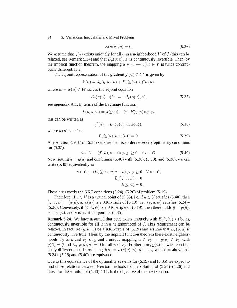
94 5. VariationalInequalitiesandMixedProblems
E(y(u), u) = 0. (5.36)
Weassumethaty(u) existsuniquelyfor all u in a neighborhoodV of C (thiscanberelaxed,seeRemark5.24)andthatEy(y(u), u) is continuouslyinvertible.Then,bythe implicit function theorem,the mappingu ∈ U 7→ y(u) ∈ Y is twice continu-ouslydifferentiable.
Theadjointrepresentationof thegradientj′(u) ∈ U∗ is givenby
j′(u) = Ju(y(u), u) +Eu(y(u), u)∗w(u),
wherew = w(u) ∈W solvestheadjointequation
Ey(y(u), u)∗w = −Jy(y(u), u), (5.37)
seeappendixA.1. In termsof theLagrangefunction
L(y, u,w) = J(y, u) + 〈w,E(y, u)〉W,W ∗
this canbewrittenasj′(u) = Lu(y(u), u,w(u)), (5.38)
wherew(u) satisfiesLy(y(u), u,w(u)) = 0. (5.39)
Any solutionu ∈ U of (5.35)satisfiesthefirst-ordernecessaryoptimalityconditionsfor (5.35):
u ∈ C, 〈j′(u), v − u〉U∗,U ≥ 0 ∀ v ∈ C. (5.40)
Now, settingy = y(u) andcombining(5.40)with (5.38),(5.39),and(5.36),we canwrite (5.40)equivalentlyas
u ∈ C, 〈Lu(y, u, w, v − u〉U∗,U ≥ 0 ∀ v ∈ C,Ly(y, u, w) = 0
E(y, u) = 0.
Theseareexactly theKKT-conditions(5.24)–(5.26)of problem(5.19).Therefore,if u ∈ U is acritical pointof (5.35),i.e. if u ∈ U satisfies(5.40),then
(y, u, w) = (y(u), u, w(u)) is a KKT-triple of (5.19),i.e., (y, u, w) satisfies(5.24)–(5.26).Conversely, if (y, u, w) is a KKT-triple of (5.19),thenthereholdsy = y(u),w = w(u), andu is acritical pointof (5.35).
Remark 5.24. We have assumedthaty(u) existsuniquelywith Ey(y(u), u) beingcontinuouslyinvertible for all u in a neighborhoodof C. This requirementcanberelaxed.In fact, let (y, u, w) bea KKT-triple of (5.19)andassumethatEy(y, u) iscontinuouslyinvertible.Then,by theimplicit functiontheoremthereexist neighbor-hoodsVU of u andVY of y anda uniquemappingu ∈ VU 7→ y(u) ∈ VY withy(u) = y andEy(y(u), u) = 0 for all u ∈ VU . Furthermore,y(u) is twice continu-ouslydifferentiable.Introducingj(u) = J(y(u), u), u ∈ VU , we seeasabove that(5.24)–(5.26)and(5.40)areequivalent.
Dueto this equivalenceof theoptimality systemsfor (5.19)and(5.35)we expecttofind closerelationsbetweenNewton methodsfor the solutionof (5.24)–(5.26)andthosefor thesolutionof (5.40).This is theobjectiveof thenext section.

5.2 MixedProblems 95
5.2.3 RelationsbetweenFull and ReducedNewtonSystem
Wenow returnto problems(5.19)with U = Lp(Ω)m and
C = u ∈ Lp(Ω)m : u(ω) ∈ C, ω ∈ Ω,whereC ⊂ Rm is closedand convex. As in Remark5.24, let us supposethat(y, u, w) is a KKT-triple with continuouslyinvertibleoperatorEy(y, u) anddenoteby y(u) thelocally uniquecontrol-to-statemappingwith y(u) = y.
We considerthe reformulation(5.27) of (5.24)–(5.26)under the Assumption5.17.If weworkwith exactelementsM of thegeneralizeddifferential∂CΣ(y, u,w),thesemismoothNewton methodfor thesolutionof (5.27)requiresto solve systemsof theformMs = −Σ(y, u,w). Accordingto Theorem5.19,thesesystemsassumetheform Lyy Lyu E∗y ρ1
D2Luy D1I +D2Luu D2E∗u ρ2
Ey Eu 0 ρ3
, (5.41)
wherewe have omitted the arguments(y, u,w) and (y, u). By the Banachtheo-rem,Ey(y, u) is continuouslyinvertiblein a neighborhoodof (y, u) with uniformlyboundedinverse.Usingthis,we canperformthefollowing block elimination: Lyy Lyu E∗y ρ1
D2Luy D1I +D2Luu D2E∗u ρ2
Ey Eu 0 ρ3
m (Row 1− LyyE−1
y × Row 3) 0 Lyu − LyyE−1y Eu E∗y ρ1 − LyyE−1
y ρ3
D2Luy D1I +D2Luu D2E∗u ρ2
Ey Eu 0 ρ3
m (Row 2−D2LuyE
−1y × Row 3) 0 Lyu − LyyE−1
y Eu E∗y ρ1 − LyyE−1y ρ3
0 D1I +D2(Luu − LuyE−1y Eu) D2E
∗u ρ2 −D2LuyE
−1y ρ3
Ey Eu 0 ρ3
m (Row 2−D2E
∗u(E∗y )−1 × Row 1) 0 Lyu − LyyE−1
y Eu E∗y ρ1 − LyyE−1y ρ3
0 D1I +D2H 0 ρ′2Ey Eu 0 ρ3
,
where
H(y, u,w) = Luu − LuyE−1y Eu −E∗u(E∗y)−1Lyu
+E∗u(E∗y )−1LyyE
−1y Eu, (5.42)

96 5. VariationalInequalitiesandMixedProblems
ρ′2 = ρ2 −D2E∗u(E
∗y )−1ρ1 +D2(E∗u(E
∗y)−1Lyy − Luy)E−1
y ρ3.
TheoperatorH canbewritten in theform
H = T ∗(Lyy LyuLuy Luu
)T, T (y, u) =
(−E−1y EuI
).
Therefore,thecontinuousinvertibility of M is closelyrelatedto thecontinuousin-vertibility of theoperatorD1I +D2H.
We now considerthereducedobjective functionj(u) = J(y(u), u) in a neigh-borhoodof u. It is shown in appendixA.1 thattheHessianj′′(u) canberepresentedin theform
j′′(u) = T (y, u)∗(Lyy(y, u,w) Lyu(y, u,w)Luy(y, u,w) Luu(y, u,w)
)T (y, u),
T (y, u) =(−Ey(y, u)−1Eu(y, u)
I
),
wherey = y(u), andw = w(u) is the adjoint state,given by the adjoint equa-tion (5.37), which can also be written in the form (5.39). Therefore,we seethatj′′(u) = H(y(u), u,w(u)) and,hence,j′′(u) = H(y, u, w), sincey = y(u) andw = w(u). For (y, u,w) = (y(u), u,w(u)) we haveLu(y(u), u,w(u)) = j′(u) by(5.38).Hence,with D = (D1|D2),
D(ω) ∈ ∂Cπ(u(ω), Lu(y(u), u,w(u))(ω)
) ⇐⇒ D(ω) ∈ ∂Cπ(u(ω), j′(u)(ω)
).
Thus,by Theorems5.11and5.19,for any (y, u,w) = (y(u), u,w(u)) andall oper-atorsM of theform (5.28)theSchurcomplementsatisfies
MR = D1I +D2H(y(u), u,w(u)) ∈ ∂CΠR(u),
whereΠR(u)(ω) = π
(u(ω), j′(u)(ω)
).
For theapplicationof theclassof (projected)semismoothNewtonmethodsto prob-lem (5.27) we needthe invertibility of Mk ∈ ∂CΣ(yk, uk, wk) as operatorbe-tweenappropriatespaces.We alreadyobserved that for the reducedproblemit isappropriateto requiretheuniformly boundedinvertibility of MR
k ∈ ∂CΠR(uk) inL([Lr]m, [Lr ]m). In agreementwith this wenow require:
Assumption 5.25. At leastoneof thefollowing conditionsholds:
(a) TheoperatorsMk ∈ ∂CΣ(yk, uk, wk) arecontinuouslyinvertibleelementsofL(Y × [Lr]m×W,Y ∗× [Lr ]m×W ∗) with thenormsof their inversesboundedby aconstantCM−1 .
(b) Thereexist constantsη > 0 andCM−1 > 0 suchthat, for all (y, u,w) ∈(y, u, w) + ηBY×[Lp]m×W , everyM ∈ ∂CΣ(yk, uk, wk) is an invertible el-ementof L(Y × [Lr]m ×W,Y ∗ × [Lr]m ×W ∗) with thenormof its inverseboundedbyCM−1 .

5.2 MixedProblems 97
Thisassumptioncorrespondsto Assumption3.11(i) with Y0 = Y × [Lr]m ×W .Under Assumptions5.17, 5.25 and 3.11 (ii) (ensuringthe availability of a
smoothingstep),we can apply Algorithm 3.9 or its projectedversion,Algorithm3.17, (with, Bk = Mk and, e.g.,K = C) for f = Σ, ∂∗f = ∂CΣ, Y =Y × [Lp]m×W ,Z = Y ∗× [Lr]m×W ∗, andY0 = Y × [Lr ]m×W . TheTheorems3.12and3.19thenguaranteesuperlinearconvergencesince,by Theorem5.19,Σ is∂CΣ-semismooth.In section5.2.4wewill proposeawayof constructingsmoothingsteps.
In thesameway, we canconsiderreformulationsarisingundertheAssumption5.20.In this casewe have
Lu(y, u,w) = λu+G(y, u,w), π(x) = x1 − PC(x1 − λ−1x2).
Further, for all M ∈ ∂CΣ(y, u,w), there exists D ∈ L∞(Ω)m×m with D ∈∂CPC(−λ−1G(y, u,w)) suchthat
M =
Lyy Lyu E∗yλ−1DGy I + λ−1DGu λ−1DGwEy Eu 0
=
Lyy Lyu E∗yλ−1DLuy I + λ−1D(Luu − λI) λ−1DE∗u
Ey Eu 0
=
Lyy Lyu E∗yD2Luy D1I +D2Luu D2E
∗u
Ey Eu 0
,
withD1 = I−D andD2 = λ−1D. Notethat(D1,D2) ∈ ∂Cπ(u,Lu(y, u,w)) and,hence,for thesechoicesof D1 andD2, the operatorM assumesthe form (5.28).Thus,we canapply the sametransformationsto the Newton systemasbeforeandobtainagainthatfor (y, u,w) = (y(u), u,w(u)) thegeneralizeddifferentialsof thereducedsemismoothreformulationappearasSchurcomplementof thefull system.As regularity conditionwechoose:
Assumption 5.26. At leastoneof thefollowing conditionsholds:
(a) TheoperatorsMk ∈ ∂CΣ(yk, uk, wk) arecontinuouslyinvertibleelementsofL(Y ×[Lr ]m×W,Y ∗×[Lr]m×W ∗) with thenormsof their inversesuniformlyboundedby aconstantCM−1 .
(b) Thereexist constantsη > 0 andCM−1 > 0 suchthat, for all (y, u,w) ∈(y, u, w) + ηBY×[Lr ]m×W , everyM ∈ ∂CΣ(yk, uk, wk) is an invertible el-ementof L(Y × [Lr]m ×W,Y ∗ × [Lr]m ×W ∗) with thenormof its inverseboundedbyCM−1 .
Thisassumptioncorrespondsto Assumption3.11(i) with Y0 = Y = Y ×[Lr]m×W .Now, underAssumptions5.20and5.26,wecanapplyAlgorithm 3.9or its projectedversion,Algorithm 3.17,for f = Σ, ∂∗f = ∂CΣ, Y = Y0 = Y × [Lr]m ×W ,

98 5. VariationalInequalitiesandMixedProblems
andZ = Y ∗ × [Lr]m × W ∗. SinceY0 = Y , we do not needa smoothingstep.Theorems3.12and3.19establishsuperlinearconvergencesince,by Theorem5.21,Σ is ∂CΣ-semismooth.
5.2.4 SmoothingSteps
In additionto Assumption5.17,we require:
Assumption 5.27. ThederivativeLu hastheformLu(y, u,w) = λu+G(y, u,w),with
(y, u,w) ∈ Y × Lr(Ω)m ×W 7→ G(y, u,w) ∈ Lp(Ω)m
beinglocally Lipschitzcontinuous.
Example5.28. Weverify thisassumptionfor thecontrolproblemof Example5.23.There,wehadY = W = H1
0 , U = Lp with p ≥ 2 arbitrary, and
Lu(y, u,w) = λu− gw = λu+G(y, u,w) with G(y, u,w) = −gw.
Sinceg ∈ L∞ andw ∈ H10 → Lq for all q ∈ [1,∞] if n = 1, all q ∈ [1,∞) if
n = 2, andall q ∈ [1, 2n/(n − 2)] if n ≥ 3, we seethatG mapsLr, with r ≥ 2arbitrary, linearandcontinuoustoLq. Thus,Assumption5.27holdsfor all p ∈ (2, q].
Wecanshow:
Theorem5.29. Let theAssumptions5.17and5.27hold.Thentheoperator
S : Y × Lr(Ω)m ×W 7→ Y × Lp(Ω)m ×W,
S(y, u,w) =
yPC(u− λ−1Lu(y, u,w))
w
,
definesa smoothingstep.
Proof. Wefirst notethat
x1 = PC(x1 − λ−1x2) ⇐⇒ x1 = PC(x1 − x2) ⇐⇒ π(x) = 0,
sothatu = PC
(u− λ−1Lu(y, u,w)
) ⇐⇒ Π(y, u,w) = 0.
Hence,for any solution(y, u, w) of (5.27),we have
S(y, u, w) = (y, u, w).
Furthermore,asin section4.1,pointwiseonΩ holds

5.2 MixedProblems 99
‖PC(u− λ−1Lu(y, u,w)
) − u‖2= ‖PC
(u− λ−1Lu(y, u,w)
)− PC(u− λ−1Lu(y, u, w))‖2
= ‖PC(−λ−1G(y, u,w)
)− PC(−λ−1G(y, u, w))‖2
≤ λ−1‖G(y, u,w) −G(y, u, w)‖2,
andthus,with CG denotingthelocal Lipschitzconstantof G near(y, u, w),
‖PC(u− λ−1Lu(y, u,w)
)− u‖[Lp]m
≤ CGcλ−1‖(y, u,w) − (y, u, w)‖Y×[Lr ]m×W ,
wherec dependsonm only. Theproof is complete,since
‖S(y, u,w)− (y, u, w)‖Y×[Lp]m×W≤ c(‖(y,w) − (y, w)‖Y×W + ‖PC
(u− λ−1Lu(y, u,w)
) − u‖[Lp]m).
ut
5.2.5 Regularity Conditions
We alreadyobserved that the all-at-onceNewton systemis closely relatedto theblack-boxNewton system.In this sectionwe show how theregularity of theall-at-onceNewton systemcanbe reducedto regularity conditionson its Schurcomple-ment.Since,for (y, u,w) = (y(u), u,w(u)), this Schurcomplementcoincideswiththeoperatorof theblack-boxNewtonsystem,sufficientconditionsfor regularitycanthenbe developedalongthe lines of section4.3. In the following, we restrictourinvestigationsto thesituationof Assumptions5.20and5.26.
Our hypothesison theSchurcomplementis:
Assumption 5.30. Thereexist constantsη > 0 andCRM−1 > 0 suchthat, for all(y, u,w) ∈ (y, u, w) + ηBY×[Lr]m×W holds:
(i) Ey(y, u,w) ∈ L(Y × [Lr]m×W,Y ∗× [Lr]m×W ∗) is continuouslyinvertiblewith uniformly boundedinverse.
(ii) For all D satisfying(5.30),theSchurcomplement
D1 +D2H,
with D1 = I − D, D2 = λ−1D, andH asdefinedin (5.42), is an invertibleelementof L([Lr]m, [Lr]m) with ‖M−1‖[Lr]m,[Lr]m ≤ CRM−1 .
Theorem5.31. Let theAssumptions5.20and5.30hold.Thentheregularity condi-tion of Assumption5.26(b) holds.
Proof. Let (y, u,w) ∈ (y, u, w) + ηBY×[Lr ]m×W andM ∈ ∂CΣ(y, u,w) be ar-bitrary. ThenthereexistsD satisfying(5.30)suchthatM assumestheform (5.29).

100 5. VariationalInequalitiesandMixedProblems
Now considerany ρ = (ρ1, ρ2, ρ3)T ∈ Y ∗×[Lr]m×W ∗. Then,accordingto section5.2.3,solvingthesystem
M(sy, su, sw)T = ρ
is equivalentto
(D1I +D2H)su = ρ2 −D2E∗u(E
∗y)−1ρ1
+D2(E∗u(E∗y)−1Lyy − Luy)E−1
y ρ3, (5.43)
Eysy = ρ3 −Eusu, (5.44)
E∗ysw = ρ1 − LyyE−1y ρ3 − (Lyu − LyyE−1
y Eu)su. (5.45)
Theassumptionsensuretwicecontinuousdifferentiabilityof L anduniformly boun-dedinvertibility of Ey andD1 + D2H. Furthermore,D andthusD1, D2 areuni-formly boundedin [L∞]m×m dueto theLipschitzcontinuityof PC . Thisand(5.43)–(5.45)show that,possiblyaftershrinkingη, thereexistsCM−1 > 0 suchthat
‖s‖Y×[Lr ]m×W ≤ CM−1‖s‖Y ∗×[Lr]m×W ∗ ,
holdsuniformly on (y, u, w) + ηBY×[Lr]m×W . ut

6. Trust-Region Globalization
Sofar, we have concentratedon locally convergentNewton-typemethods.We nowproposea classof trust-region algorithmswhich are globally convergentand use(projected)Newton stepsascandidatesfor trial steps.Hereby, we restrictourselftothecasewheretheproblemis posedin Hilbert space,which, from a practicalpointof view, is notvery restrictive.
To motivateour approach,weconsider(1.1)with U = L2(Ω) andcontinuouslydifferentiablefunctionF : U → U . UsinganMCP/NCP-functionφ, wereformulatetheproblemin theform
Φ(u) = 0. (6.1)
Let theAssumption5.1holdwith r = 2 andsomep, p′ ∈ (2,∞]. ThentheoperatorΦ : Lp(Ω) → L2(Ω) is semismoothby Theorem5.4. Alternatively, if F assumestheformF (u) = λu+G(u) andG hasthesmoothingpropertyof section4.2,andifΦ(u) = u−PB(u−λ−1G(u)) is chosen,thenby Theorem4.4,Φ : L2(Ω)→ L2(Ω)is is locally Lipschitzcontinuousandsemismooth.
For globalization,we needa minimizationproblemwhosesolutionsor criticalpoints correspondto solutionsof (6.1). We proposethreedifferentapproachestoobtaintheseminimizationreformulations:
Most naturally, wecanchoosethesquaredresidual
h(u) =12‖Φ(u)‖2L2
asobjective function.In fact,any globalsolutionof h is a solutionto Φ(u) = 0 andviceversa.Therefore,(6.1) is equivalentto theminimizationproblem
minimizeu∈L2(Ω)
h(u). (6.2)
We will show that, for appropriatechoicesof φ, the functionh(u) = ‖Φ(u)‖2L2/2is continuouslydifferentiable.This makes(6.2) aC1 problemposedin theHilbertspaceL2(Ω).
As wasdiscussedin the context of the projectedsemismoothNewton method(Algorithm 3.17),it is oftendesirablethat thealgorithmstaysfeasiblewith respectto a givenclosedconvex setK ⊂ Lp(Ω) which containsthesolutionu ∈ Lp(Ω).UsuallyK = B is chosen.Weconsidersetsof thegeneralformK = aK ≤ u ≤ bKwith lower and upperboundfunctionssatisfyingthe conditions(3.46). Then theconstrainedminimizationproblem

102 6. Trust-Region Globalization
minimizeu∈L2(Ω)
h(u) subjectto u ∈ K (6.3)
is equivalentto (6.1)in thesensethatany globalsolutionu ∈ K of (6.3)solves(6.1)andviceversa.
Finally, we cometo a third possibility of globalization,which can be usediftheVIP is obtainedfrom thefirst-ordernecessaryoptimality conditionsof thecon-strainedminimizationproblem
minimize j(u) subjectto u ∈ B (6.4)
with B = u ∈ L2(Ω) : a ≤ u ≤ b asin (1.1).Thenwe canusetheproblem(6.4)itself for thepurposeof globalization.
In all threeapproaches,(6.2),(6.3),and(6.4),weobtainaminimizationproblemof theform
minimizeu∈L2(Ω)
f(u) subjectto u ∈ K. (6.5)
For thedevelopmentandanalysisof thetrust-regionmethod,ratherthanworkingin L2, wepreferto chooseageneralHilbert spacesetting.Thishastheadvantageofcoveringalsothefinite-dimensionalcase,andmany othersituations,e.g.,therefor-mulationof mixedproblems,seesection5.2.Therefore,in thefollowing weconsidertheproblem
minimizeu∈U
f(u) subjectto u ∈ K, (6.6)
wheref : U → R is a continuouslydifferentiablefunction that is definedon theHilbert spaceU . The feasiblesetK ⊂ U is assumedto be nonempty, closed,andconvex. In particular, thereexistsauniquemetricprojection
PK : U → K, PK(u) = argminv∈K
‖v − u‖U .
Weidentify thedualU∗ of U with U , i.e.,we use〈·, ·〉U∗,U = (·, ·)UOurideais to useprojectedsemismoothNewtonstepsastrial stepcandidatesfor
atrust-regionglobalizationbasedon(6.6).In general,thepresenceof thesmoothingstepin thesemismoothNewton methodmakesit difficult to prove rigorouslytran-sition to fastlocal convergence.Therearewaysto do this, but theapproachwouldbehighly technical,andthuswe will prove transitionto fastlocal convergenceonlyfor thecasewherethesemismoothNewtonmethodconvergessuperlinearlywithouta smoothingstep.This is justifiedfor two reasons:As we will seein our numericaltests,experienceshows that we usuallyobserve fastconvergencewithout incorpo-rating a smoothingstepin the algorithm.One reasonfor this is that a discretiza-tion would have to be very fine to resolve functionsthat yield an excessively big‖ · ‖Lp/‖ · ‖L2-ratio. Second,in section4.2 we have developeda reformulationtowhich thesemismoothNewtonmethodis applicablewithouta smoothingstep.
For unconstrainedproblems,globalconvergenceusuallymeansthatthemethod“converges”to a critical point, i.e., a pointu ∈ U suchthatf ′(u) = 0 in thesensethat at least lim infk→∞ ‖f ′(uk)‖U = 0. In the constrainedcontext, we have toclarify whatwemeanby acritical point.

6. Trust-Region Globalization 103
Definition 6.1. We call u ∈ U a critical point of (6.6) if
u ∈ K and (f ′(u), v − u)U ≥ 0 ∀ v ∈ K. (6.7)
Thefollowing resultis important:
Lemma 6.2.
(i) Letu bea local solutionof (6.6); moreprecisely, u ∈ K andthereexistsδ > 0such thatf(v) ≥ f(u) for all v ∈ (u+ δBU ) ∩ K. Thenu is a critical point of(6.6).
(ii) Thefollowingstatementsareequivalent:
(a) u is a critical pointof (6.6).
(b) u− PK(u− f ′(u)) = 0.
(c) u− PK(u− tf ′(u)) = 0 for somet > 0.
(d) u− PK(u− tf ′(u)) = 0 for all t ≥ 0.
Proof. (seealso[66, §8]).(i): For any v ∈ K, thereholdsv(t) = u + t(y − u) ∈ (u + δBU ) ∩ K for
sufficiently smallt > 0 andthus
0 ≤ [f(v(t))− f(u)]/t→ (f ′(u), v − u)U as t→ 0+.
(ii): Let t > 0 bearbitrary. Condition(6.7) is equivalentto
u ∈ K, (u− (u− tf ′(u)), v − u)U ≥ 0 ∀ v ∈ K,
which is thesameasu = PK(u− tf ′(u)). Thisprovestheequivalenceof (a)–(d).ut
Next, we introducetheconceptof criticality measures.
Definition 6.3. A continuousfunctionχ : K → [0,∞) with theproperty
χ(u) = 0⇐⇒ u is acritical pointof problem(6.6) (6.8)
is calledcriticality measure for (6.6).
Example6.4. By Lemma6.2,for any t > 0, thefunction
χP,t(u) = ‖u− PK(u− tf ′(u))‖Uis acriticality measurefor (6.6).For t = 1, theresultingcriticality measure
χP (u) = χP,1(u) = ‖u− PK(u− f ′(u))‖Uis thenormof theprojectedgradient.

104 6. Trust-Region Globalization
The algorithmthat we presentin this chapterusesideasdevelopedin the author’spaper[140] on trust-region methodsfor finite-dimensionalsemismoothequations.Othertrust-region approachesfor thesolutionof finite-dimensionalNCPsandVIPscanbefoundin, e.g.,[88, 93,119]. Trust-regionalgorithmsfor infinite-dimensionalconstrainedoptimization problemsare investigatedin, e.g., [96, 136, 144]. Themethodwe proposeallows for nonmonotonicityof thesequenceof generatedfunc-tion values.This hasprovenadvantageousto avoid convergenceto local, but non-globalsolutionsof theproblem[28, 65, 93, 137, 140].
Before we describethe trust-region algorithm, we show that for appropriatechoiceof φ the function h(u) = ‖Φ(u)‖2L2/2 is continuouslydifferentiable.Webegin with thefollowing result:
Lemma 6.5. Letψ : V → R belocally Lipschitzcontinuouson thenonemptyopensetV ⊂ Rm. Assumethatψ is continuouslydifferentiableonV \ ψ−1(0). Thenthefunctionψ2 is continuouslydifferentiableon V . Moreover, (ψ2)′(x) = 2ψ(x)g forall g ∈ ∂ψ(x) andall x ∈ V .
Thesimpleproof canbefoundin [140].
Lemma 6.6. Let ψ : Rm → R be Lipschitz continuouson Rm and continuouslydifferentiableon Rm \ ψ−1(0). Further, let G : U 7→ L2(Ω)m be continuouslydifferentiable. Thenthefunction
h : u ∈ U 7→ 12‖Ψ(u)‖2L2(Ω)m with Ψ(u)(ω) = ψ(G(u)(ω)), ω ∈ Ω,
is continuouslydifferentiablewith
h′(u) = M∗Ψ(u) ∀M ∈ ∂Ψ(u).
Remark 6.7. Notethat∂Ψ(u) ⊂ L(U,L2) by Lemma3.37.
Proof. Using Lemma6.5, η = ψ2/2 is continuouslydifferentiablewith η′(x) =ψ(x)g for all g ∈ ∂ψ(x). TheLipschitzcontinuityof ψ implies
‖η′(x)‖2 = |ψ(x)|‖g‖2 ≤ L(|ψ(0)|+ |ψ(x) − ψ(0)|) ≤ L|ψ(0)|+ L2‖x‖2.Hence,by PropositionA.10, thesuperpositionoperator
T : w ∈ L2(Ω)m 7→ η(w) ∈ L1(Ω)m
is continuouslydifferentiablewith derivative
(T ′(w)v)(ω) = η′(w(ω))v(ω) = ψ(w(ω))gT v(ω) ∀gT ∈ ∂ψ(w(ω)).
From this and the chain rule we seethatH : u ∈ U 7→ (G(u)) ∈ L1(Ω)m iscontinuouslydifferentiablewith
(H ′(u)v)(ω) = η′(G(u)(ω))(G′(u)v)(ω)
= ψ(G(u)(ω))gT (G′(u)v)(ω) ∀gT ∈ ∂ψ(G(u)(ω)).
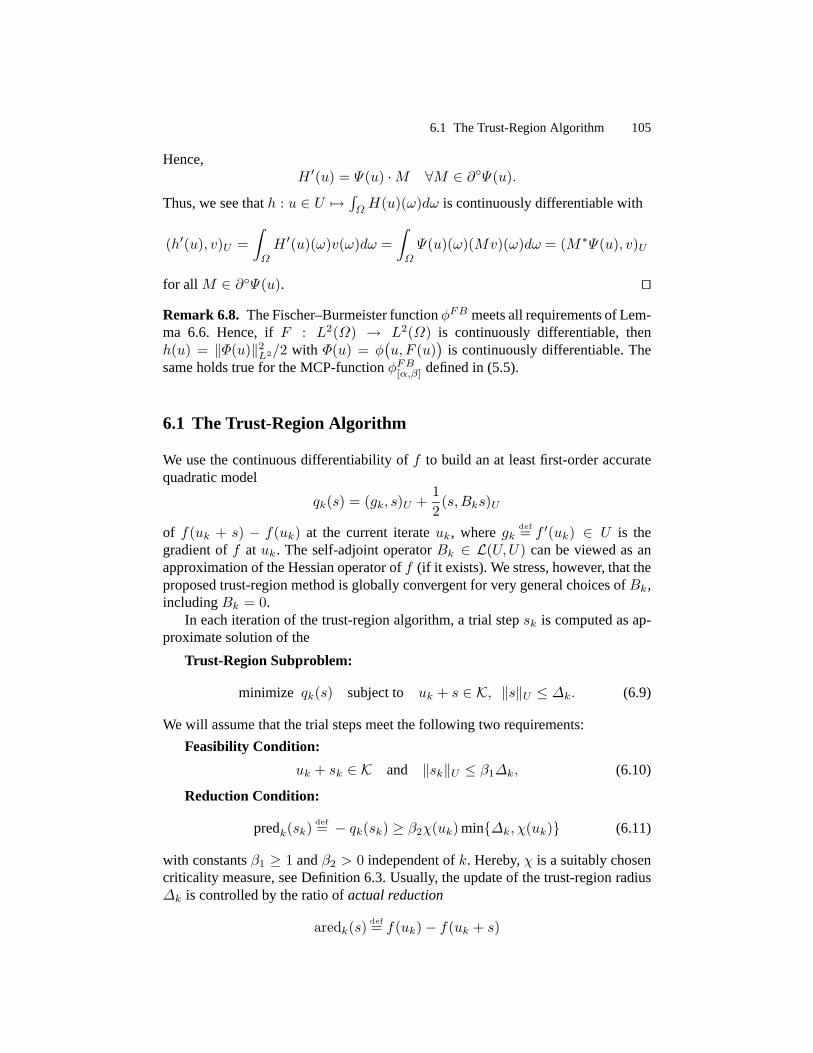
6.1 TheTrust-Region Algorithm 105
Hence,H ′(u) = Ψ(u) ·M ∀M ∈ ∂Ψ(u).
Thus,we seethath : u ∈ U 7→ ∫ΩH(u)(ω)dω is continuouslydifferentiablewith
(h′(u), v)U =∫Ω
H ′(u)(ω)v(ω)dω =∫Ω
Ψ(u)(ω)(Mv)(ω)dω = (M∗Ψ(u), v)U
for all M ∈ ∂Ψ(u). utRemark 6.8. TheFischer–BurmeisterfunctionφFB meetsall requirementsof Lem-ma 6.6. Hence, if F : L2(Ω) → L2(Ω) is continuouslydifferentiable,thenh(u) = ‖Φ(u)‖2L2/2 with Φ(u) = φ
(u,F (u)
)is continuouslydifferentiable.The
sameholdstruefor theMCP-functionφFB[α,β] definedin (5.5).
6.1 The Trust-RegionAlgorithm
We usethe continuousdifferentiabilityof f to build anat leastfirst-orderaccuratequadraticmodel
qk(s) = (gk, s)U +12(s,Bks)U
of f(uk + s) − f(uk) at the current iterateuk, wheregkdef= f ′(uk) ∈ U is the
gradientof f at uk. The self-adjointoperatorBk ∈ L(U,U) canbe viewed asanapproximationof theHessianoperatorof f (if it exists).Westress,however, thattheproposedtrust-regionmethodis globallyconvergentfor verygeneralchoicesof Bk,includingBk = 0.
In eachiterationof thetrust-region algorithm,a trial stepsk is computedasap-proximatesolutionof the
Trust-Region Subproblem:
minimize qk(s) subjectto uk + s ∈ K, ‖s‖U ≤ ∆k. (6.9)
Wewill assumethatthetrial stepsmeetthefollowing two requirements:
Feasibility Condition:
uk + sk ∈ K and ‖sk‖U ≤ β1∆k, (6.10)
Reduction Condition:
predk(sk)def= − qk(sk) ≥ β2χ(uk) min∆k, χ(uk) (6.11)
with constantsβ1 ≥ 1 andβ2 > 0 independentof k. Hereby, χ is a suitablychosencriticality measure,seeDefinition 6.3.Usually, theupdateof thetrust-region radius∆k is controlledby theratio of actualreduction
aredk(s)def= f(uk)− f(uk + s)

106 6. Trust-Region Globalization
andpredictedreductionpredk(s)def= − qk(s).
It hasbeenobserved [28, 65, 93, 137] that the performanceof nonlinearpro-grammingalgorithmscan be significantly improved by using nonmonotonelinesearch-or trust-region techniques.Hereby, in contrastto the traditionalapproach,the monotonicityf(uk+1) ≤ f(uk) of the function valuesis not enforcedin ev-ery iteration.To achieve this, we generalizea nonmonotonetrust-region techniquethatwasrecentlyintroducedby theauthor[140] in thecontext of finite-dimensionalsemismoothequations.For this algorithmall global convergenceresultsfor mono-tone,finite-dimensionaltrust-region methodsremainvalid. However, the decreaserequirementis significantlyrelaxed.Beforewe describethis approachandthecor-respondingreductionratio ρk(s) in detail,we first statethebasictrust-region algo-rithm.
Algorithm 6.9 (Trust-Region Algorithm).
1. Initialization: Chooseη1 ∈ (0, 1), ∆min ≥ 0, and a criticality measureχ.Chooseu0 ∈ K, ∆0 > 0 such that ∆0 ≥ ∆min, and a model HessianB0 ∈ L(U,U). Chooseanintegerm ≥ 1 andfix λ ∈ (0, 1/m] for thecompu-tationof ρk. Setk := 0 andi := −1.
2. Computeχk := χ(uk). If χk = 0, thenSTOP.
3. Computea trial stepsk satisfyingtheconditions(6.10)and(6.11).
4. Computethe reductionratio ρk := ρk(sk) by calling Algorithm 6.11 withmk := mini+ 1,m.
5. Computethenew trust-region radius∆k+1 by invokingAlgorithm 6.10.
6. If ρk ≤ η1, thenrejectthestepsk, i.e.,setuk+1 := uk,Bk+1 := Bk, incrementk by 1, andgo to Step3.
7. Acceptthestep:Setuk+1 := uk + sk andchooseanew modelHessianBk+1 ∈L(U,U). Setji+1 := k, incrementk andi by 1 andgo to Step2.
Theincreasingsequence(ji)i≥0, enumeratesall indicesof acceptedsteps.Moreover,
uk = uji ∀ ji−1 < k ≤ ji, ∀ i ≥ 1. (6.12)
Conversely, if k 6= ji for all i, thensk wasrejected.In thefollowing we denotethesetof all these“successful”indicesji by S:
S def= ji : i ≥ 0 = k : trial stepsk is accepted.Sometimes,acceptedstepswill alsobecalledsuccessful.Wewill repeatedlyusethefactthat
uk : k ≥ 0 = uk : k ∈ S.The trust-region updatesareimplementedasusual.We dealwith two differentfla-vors of updaterulessimultaneouslyby introducinga nonnegative parameter∆min.We requirethat after successfulsteps∆k+1 ≥ ∆min holds.If ∆min = 0 is chosen,this is automaticallysatisfied.For∆min > 0, however, it is anadditionalfeaturethatallows for specialproof techniques.

6.1 TheTrust-Region Algorithm 107
Algorithm 6.10 (Update of the Trust-Region Radius).
∆min ≥ 0 andη1 ∈ (0, 1) aretheconstantsdefinedin Step1 of Algorithm 6.9.
Let η1 < η2 < 1, and0 ≤ γ0 < γ1 < 1 < γ2 befixed.
1. If ρk ≤ η1, thenchoose
∆k+1 ∈ (γ0∆k, γ1∆k].2. If ρk ∈ (η1, η2), thenchoose
∆k+1 ∈ [γ1∆k,max∆min,∆k] ∩ [∆min,∞).3. If ρk ≥ η2, thenchoose
∆k+1 ∈ (∆k,max∆min, γ2∆k] ∩ [∆min,∞).
Westill haveto describehow thereductionratiosρk(s) aredefined.Hereisadetaileddescription:
Algorithm 6.11 (Computation of RelaxedReduction Ratio).
1. Choosescalars
λkr ≥ λ, r = 0, . . . ,mk − 1,mk−1∑r=0
λkr = 1.
2. Computetherelaxedactualreductionraredk := raredk(sk), where
raredk(s)def= max
f(uk),
mk−1∑r=0
λkrf(uji−r)
− f(uk + s). (6.13)
3. Computethereductionratioρk := ρk(sk) accordingto
ρk(s)def=
raredk(s)predk(s)
.
Remark 6.12. At the very beginning of Algorithm 6.9, Step4 invokesAlgorithm6.11with mk = 0. In this casethesumin (6.13)is emptyandthus
raredk(s) = maxf(uk), 0 − f(uk + s) = f(uk)− f(uk + s) = aredk(s).
Theideabehindtheaboveupdaterule is thefollowing: Insteadof requiringthatf(uk+sk) besmallerthanf(uk), it isonly requiredthatf(uk+sk) is eitherlessthanf(uk) or lessthantheweightedmeanof thefunctionvaluesatthelastmk = mini+1,m successfuliterates.Of course,if m = 1, thenraredk(s) = aredk(s) andtheusualreductionratio is recovered.Our approachis a slightly strongerrequirementthanthestraightforwardideato replacearedk with
rared∞k (s) = max0≤r<mk
f(uji−r)− f(uk + s).

108 6. Trust-Region Globalization
Unfortunately, for this latter choiceit doesnot seemto be possibleto establishalltheglobalconvergenceresultsthatareavailablefor themonotonecase.For our ap-proach,however, this is possiblewithout makingthe theorysubstantiallymoredif-ficult. Moreover, we can approximaterared∞k arbitrarily accuratelyby raredk ifwe chooseλ sufficiently small, in eachiteration select0 ≤ rk < mk satisfyingf(uji−rk
) = max0≤r<mk
f(uji−r), andset
λkr = λ if r 6= rk, λkrk= 1− (mk − 1)λ. (6.14)
6.2 Global Convergence
For theglobalconvergenceanalysiswe rely on thefollowing
Assumption 6.13.
(i) Theobjectivefunctionf is continuouslydifferentiableonanopenneighborhoodof thenonemptyclosedconvex setK.
(ii) Thefunctionf is boundedbelow onK.
(iii) Thenormsof themodelHessiansareuniformly bounded:
‖Bk‖U,U ≤ CB for all k.
Throughoutthis section,Assumption6.13is requiredto hold.Wefirst proveanimportantdecreasepropertyof thefunctionvaluesf(uk).
Lemma 6.14. Let uk, sk, ∆k, ji, etc.,begeneratedby Algorithm6.9. Thenfor allcomputedindicesi ≥ 1 holds
f(uji) < f(u0)− η1λi−2∑r=0
predjr(sjr)− η1predji−1(sji−1) < f(u0). (6.15)
Proof. We will usetheshortnotationsaredk = aredk(sk), raredk = raredk(sk),andpredk = predk(sk). First, let usnotethat (6.11)impliespredk > 0 wheneveruk is notcritical. Therefore,thesecondinequalityholds.
Theproofof thefirst inequalityis by induction.For i = 1 wehaveby (6.12)andusingρj0(sj0) > η1
f(uj1) = f(uj0+1) = f(uj0)− aredj0 < f(uj0)− η1predj0 = f(u0)− η1predj0 .
Now assumethat(6.15)holdsfor 1, . . . , i.If raredji = aredji then,using(6.15)andλ ≤ 1,
f(uji+1) = f(uji+1) = f(uji)− aredji = f(uji)− raredji
< f(u0)− η1λi−2∑r=0
predjr − η1predji−1− η1predji
≤ f(u0)− η1λi−1∑r=0
predjr − η1predji .
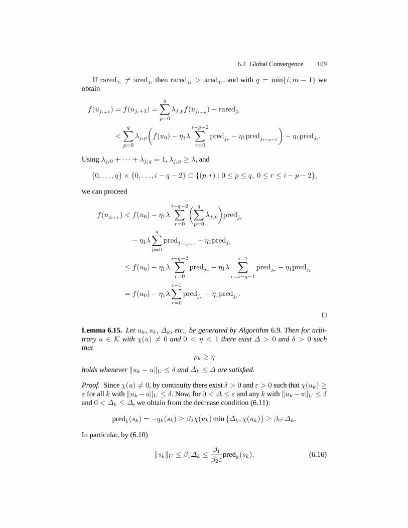
6.2 GlobalConvergence 109
If raredji 6= aredji thenraredji > aredji , andwith q = mini,m − 1 weobtain
f(uji+1) = f(uji+1) =q∑p=0
λjipf(uji−p)− raredji
<
q∑p=0
λjip
(f(u0)− η1λ
i−p−2∑r=0
predjr − η1predji−p−1
)− η1predji .
Usingλji0 + · · · + λjiq = 1, λjip ≥ λ, and
0, . . . , q × 0, . . . , i − q − 2 ⊂ (p, r) : 0 ≤ p ≤ q, 0 ≤ r ≤ i− p− 2,
wecanproceed
f(uji+1) < f(u0)− η1λi−q−2∑r=0
( q∑p=0
λjip
)predjr
− η1λq∑p=0
predji−p−1− η1predji
≤ f(u0)− η1λi−q−2∑r=0
predjr − η1λi−1∑
r=i−q−1
predjr − η1predji
= f(u0)− η1λi−1∑r=0
predjr − η1predji .
utLemma 6.15. Let uk, sk, ∆k, etc.,be generatedby Algorithm 6.9. Thenfor arbi-trary u ∈ K with χ(u) 6= 0 and 0 < η < 1 there exist∆ > 0 and δ > 0 suchthat
ρk ≥ ηholdswhenever‖uk − u‖U ≤ δ and∆k ≤ ∆ aresatisfied.
Proof. Sinceχ(u) 6= 0, by continuitythereexist δ > 0 andε > 0 suchthatχ(uk) ≥ε for all k with ‖uk−u‖U ≤ δ. Now, for 0 < ∆ ≤ ε andany k with ‖uk−u‖U ≤ δand0 < ∆k ≤ ∆, weobtainfrom thedecreasecondition(6.11):
predk(sk) = −qk(sk) ≥ β2χ(uk) min∆k, χ(uk) ≥ β2ε∆k.
In particular, by (6.10)
‖sk‖U ≤ β1∆k ≤ β1
β2εpredk(sk). (6.16)

110 6. Trust-Region Globalization
Further, with appropriateyk = uk + τksk, τk ∈ [0, 1], by the intermediatevaluetheorem
aredk(sk) = f(uk)− f(uk + sk) = −(f ′(yk), sk)U
= −qk(s) + (gk − f ′(yk), sk)U +12(sk, Bksk)U
≥ predk(sk)−(‖gk − f ′(yk)‖U +
12‖Bksk‖U
)‖sk‖U .
Sincef ′ is continuous,thereexistsδ′ > 0 suchthat
‖f ′(u′)− f ′(u)‖U ≤ (1− η)β2ε
4β1
for all u′ ∈ K with ‖u′ − u‖U < δ′. Further, since‖Bk‖U,U ≤ CB by Assumption6.13(iii), choosing∆ sufficiently smallyields
12‖Bksk‖U ≤ (1− η)β2ε
2β1.
for all k with ∆k ≤ ∆. By reducing∆ andδ, if necessary, suchthatδ + β1∆ < δ′
weachieve,using(6.10),thatfor all k with ‖uk − u‖U ≤ δ and0 < ∆k ≤ ∆
‖yk − u‖U ≤ ‖uk − u‖U + τk‖sk‖U ≤ δ + β1∆ < δ′, ‖uk − u‖U ≤ δ < δ′.
Hence,for all theseindicesk,
‖gk − f ′(yk)‖U ≤ ‖gk − f ′(u)‖U + ‖f ′(u)− f ′(yk)‖U ≤ (1− η)β2ε
2β1,
andthusby (6.16)(‖gk − f ′(yk)‖U +
12‖Bksk‖U
)‖sk‖U ≤ (1− η)β2ε
β1‖sk‖U
≤ (1− η)predk(sk).
This impliesthatfor all thesek thereholds
raredk(sk) ≥ aredk(sk) ≥ predk(sk)−(‖gk − f ′(yk)‖U +
12‖Bksk‖U
)‖sk‖U
≥ ηpredk(sk).
Theproof is complete. utLemma 6.16. Algorithm6.9eitherterminatesafter finitely manystepswith a criti-cal pointuk of (6.6)or generatesan infinitesequence(sji) of acceptedsteps.

6.2 GlobalConvergence 111
Proof. Assumethat Algorithm 6.9 neitherterminatesnor generatesan infinite se-quence(sji) of acceptedsteps.Thenthereexists a smallestindex k0 suchthat allstepssk arerejectedfor k ≥ k0. In particular, uk = uk0 , k ≥ k0, andthesequenceof trust-region radii∆k tendsto zeroask →∞, because
∆k0+j ≤ γj1∆k0 .
Sincethealgorithmdoesnot terminate,we know thatχ(uk0) 6= 0. But now Lemma6.15 with u = uk0 yields that sk is acceptedassoonas∆k becomessufficientlysmall. This contradictsour assumption.Therefore,the assertionof the Lemmaistrue. utLemma 6.17. Assumethat Algorithm6.9generatesinfinitelymanysuccessfulstepssji andthat thereexistsS ′ ⊂ S with∑
k∈S′∆k =∞. (6.17)
Then lim infS′3k→∞
χ(uk) = 0.
Proof. Let the assumptionsof the lemma hold and assumethat the assertioniswrong. Thenthereexists ε > 0 suchthatχ(uk) ≥ ε for all k ∈ S ′ ⊂ S. From(6.17)follows thatS ′ is not finite. For all k ∈ S ′ holdsby (6.11)
predk(sk) ≥ β2χ(uk) min∆k, χ(uk) ≥ β2εmin∆k, ε .
Fromthisestimate,thefactthatf is boundedbelow onK, seeAssumption6.13(ii),andLemma6.14we obtainfor all j ∈ S ′, usingλ ≤ 1
f(u0)− f(uj) > η1λ∑k∈Sk<j
predk(sk) ≥ η1λ∑k∈S′k<j
predk(sk)
≥ η1λβ2ε∑k∈S′k<j
min∆k, ε → ∞ (asj →∞).
This is a contradiction.Therefore,the assumptionwas wrong and the lemmaisproved. ut
Wenow haveeverythingathandthatweneedto establishourfirst globalconver-genceresult.It is applicablein thecaseγ0 > 0,∆min > 0 andsaysthataccumulationpointsarecritical pointsof (6.6).
Theorem6.18. Letγ0 > 0 and∆min > 0. Assumethat Algorithm6.9doesnot ter-minateafter finitely manystepswith a critical pointuk of (6.6). Thenthealgorithmgeneratesinfinitely manyacceptedsteps(sji). Moreover, everyaccumulationpointof (uk) is a critical point of (6.6).

112 6. Trust-Region Globalization
Proof. SupposethatAlgorithm 6.9doesnot terminateafterafinite numberof steps.Thenaccordingto Lemma6.16infinitely many successfulsteps(sji) aregenerated.Assumethat u is anaccumulationpoint of (uk) that is not a critical point of (6.6).Sinceχ(u) 6= 0, invokingLemma6.15with u = u yields∆ > 0 andδ > 0 suchthatk ∈ S holdsfor all k with ‖uk − u‖ ≤ δ and∆k ≤ ∆. Sinceu is anaccumulationpoint, thereexists an infinite increasingsequencej′i ∈ S, i ≥ 0, of indicessuch‖uj′i − u‖ ≤ δ anduj′i → u.
If (j′i − 1) ∈ S, then∆j′i ≥ ∆min. Otherwise,sj′i−1 wasrejected,which, sincethenuj′i−1 = uj′i , is only possibleif ∆j′i−1 > ∆, andtherefore∆j′i ≥ γ0∆j′i−1 >γ0∆. We concludethatfor all i holds∆j′i ≥ min∆min, γ0∆. Now Lemma6.17isapplicablewith S ′ = j′i : i ≥ 0 andyields
0 6= χ(u) = limi→∞
χ(uj′i) = lim infi→∞
χ(uj′i) = 0,
wherewe have usedthecontinuityof χ. This is a contradiction.Therefore,theas-sumptionχ(u) 6= 0 waswrong. ut
Next, weprovea resultthatholdsalsofor ∆min = 0. Moreover, theexistenceofaccumulationpointsis not required.
Theorem6.19. Let γ0 > 0 or ∆min = 0 hold. Assumethat Algorithm 6.9 doesnot terminateafter finitely manystepswith a critical point uk of (6.6). Thenthealgorithmgeneratesinfinitelymanyacceptedsteps(sji). Moreover,
lim infk→∞
χ(uk) = 0. (6.18)
In particular, if uk convergesto u, thenu is a critical pointof (6.6).
Proof. By Lemma6.16,infinitely many successfulsteps(sji) aregenerated.Nowassumethat(6.18)is wrong,i.e.,
lim infk→∞
χ(uk) > 0. (6.19)
Thenweobtainfrom Lemma6.17that∑k∈S
∆k <∞. (6.20)
In particular, (uji) is a Cauchysequenceby (6.10)and(6.12).Therefore,(uk) con-vergesto somelimit u, at which accordingto (6.19)andthe continuity of χ holdsχ(u) 6= 0.Case1:∆min > 0.
Thenby assumptionalsoγ0 > 0, andTheorem6.18yieldsχ(u) = 0, which is acontradiction.Case2:∆min = 0.
Lemma6.15with u = u andη = η2 yields∆ > 0 andδ > 0 suchthatk ∈ Sand∆k+1 ≥ ∆k holdsfor all k with ‖uk − u‖ ≤ δ and∆k ≤ ∆. Sinceuk → u,
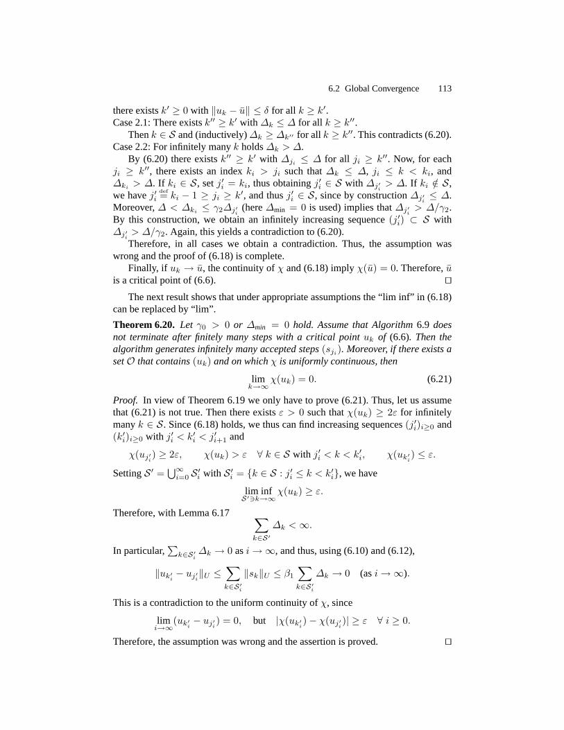
6.2 GlobalConvergence 113
thereexistsk′ ≥ 0 with ‖uk − u‖ ≤ δ for all k ≥ k′.Case2.1:Thereexistsk′′ ≥ k′ with ∆k ≤ ∆ for all k ≥ k′′.
Thenk ∈ S and(inductively)∆k ≥ ∆k′′ for all k ≥ k′′. Thiscontradicts(6.20).Case2.2:For infinitely many k holds∆k > ∆.
By (6.20) thereexistsk′′ ≥ k′ with ∆ji ≤ ∆ for all ji ≥ k′′. Now, for eachji ≥ k′′, thereexists an index ki > ji suchthat∆k ≤ ∆, ji ≤ k < ki, and∆ki
> ∆. If ki ∈ S, setj′i = ki, thusobtainingj′i ∈ S with ∆j′i > ∆. If ki /∈ S,we have j′i
def= ki − 1 ≥ ji ≥ k′, andthusj′i ∈ S, sinceby construction∆j′i ≤ ∆.Moreover, ∆ < ∆ki
≤ γ2∆j′i (here∆min = 0 is used)implies that∆j′i > ∆/γ2.By this construction,we obtain an infinitely increasingsequence(j′i) ⊂ S with∆j′i > ∆/γ2. Again, this yieldsacontradictionto (6.20).
Therefore,in all caseswe obtain a contradiction.Thus, the assumptionwaswrongandtheproof of (6.18)is complete.
Finally, if uk → u, thecontinuityof χ and(6.18)imply χ(u) = 0. Therefore,uis acritical pointof (6.6). ut
Thenext resultshowsthatunderappropriateassumptionsthe“lim inf” in (6.18)canbereplacedby “lim”.
Theorem6.20. Let γ0 > 0 or ∆min = 0 hold. Assumethat Algorithm 6.9 doesnot terminateafter finitely manystepswith a critical point uk of (6.6). Thenthealgorithmgeneratesinfinitely manyacceptedsteps(sji). Moreover, if thereexistsasetO that contains(uk) andonwhichχ is uniformlycontinuous,then
limk→∞
χ(uk) = 0. (6.21)
Proof. In view of Theorem6.19we only have to prove (6.21).Thus,let usassumethat (6.21) is not true.Thenthereexistsε > 0 suchthatχ(uk) ≥ 2ε for infinitelymany k ∈ S. Since(6.18)holds,we thuscanfind increasingsequences(j′i)i≥0 and(k′i)i≥0 with j′i < k′i < j′i+1 and
χ(uj′i) ≥ 2ε, χ(uk) > ε ∀ k ∈ S with j′i < k < k′i, χ(uk′i) ≤ ε.SettingS ′ =
⋃∞i=0 S ′i with S ′i = k ∈ S : j′i ≤ k < k′i, we have
lim infS′3k→∞
χ(uk) ≥ ε.Therefore,with Lemma6.17 ∑
k∈S′∆k <∞.
In particular,∑k∈S′i ∆k → 0 asi→∞, andthus,using(6.10)and(6.12),
‖uk′i − uj′i‖U ≤∑k∈S′i‖sk‖U ≤ β1
∑k∈S′i
∆k → 0 (asi→∞).
This is acontradictionto theuniform continuityof χ, since
limi→∞
(uk′i − uj′i) = 0, but |χ(uk′i)− χ(uj′i)| ≥ ε ∀ i ≥ 0.
Therefore,theassumptionwaswrongandtheassertionis proved. ut
114 6. Trust-Region Globalization
6.3 ImplementableDecreaseConditions
Algorithm6.9requiresthecomputationof trial stepsthatsatisfytheconditions(6.10)and (6.11). We now describehow thesecondition can be implementedby meansof a generalizedCauchypoint which is basedon the projectedgradientpath.Ascriticality measurewe can useany criticality measureχ that is majorizedby theprojectedgradientin thefollowing sense:
θχ(u) ≤ χP (u) def= ‖u− PK(u− f ′(u))‖U (6.22)
with a fixedparameterθ > 0. For uk ∈ K andt ≥ 0, we introducethe projectedgradientpath
πk(t) = PK(uk − tgk)− uk.anddefinethegeneralizedCauchy point sck asfollows:
sck = πk(σk), with σk ∈ 1, 2−1, 2−2, . . . chosenmaximalsuchthat
qk(πk(σk)) ≤ γ(gk, πk(σk))U , (6.23)
‖πk(σk)‖U ≤ ∆k, (6.24)
whereγ ∈ (0, 1) is afixedparameter.Our aim is to show that the following conditionensuresthat (6.11) is satisfied
with a constantβ2 independentof uk.
Fraction of Cauchy DecreaseCondition:
predk(sk) ≥ β3predk(sck), (6.25)
whereβ3 ∈ (0, 1] is fixed.Wefirst establishseveralusefulpropertiesof theprojectedgradientpath.
Lemma 6.21. Letuk ∈ K. Thenfor all t ∈ (0, 1] andall s ≥ 1 holds
‖πk(t)‖U ≤ ‖πk(st)‖U ≤ s‖π(t)‖U , (6.26)
−(gk, πk(t))U ≥ 1t‖πk(t)‖2U ≥ χP (uk)‖πk(t)‖U ≥ tχP (uk)2, (6.27)
Proof. The first inequality in (6.26) is well known, see,e.g., [136, Lem. 2]. Thesecondinequalityis provedin [27]. For (6.27),we usethat
(PK(v)− v, u− PK(v))U ≥ 0 ∀ u ∈ K, v ∈ U, (6.28)
sincew = PK(v) minimizes‖w − v‖2U onK. Wesetvk(t) = uk − tgk andderive
−(tgk, πk(t))U = (πk(t) + [(vk(t)− PK(vk(t))], πk(t))U= ‖πk(t)‖2 + (vk(t)− PK(vk(t)), PK(vk(t))− uk) ≥ ‖πk(t)‖2,
wherewehaveused(6.28)in thelaststep.FromχP (uk) = πk(1) and(6.26)followtheremainingassertions. ut

6.3 ImplementableDecreaseConditions 115
Thisallowsusto prove thewell-definednessof thegeneralizedCauchypoint.
Lemma 6.22. For all uk ∈ K, thecondition(6.23)is satisfiedwhenever
0 < σk ≤ σ0 def= min
1,
2(1− γ)CB
.
Furthermore, thecondition(6.24)holdsfor all σk ∈ (0, 1] with
σk‖gk‖U ≤ ∆k.
Proof. For all 0 < t ≤ σ0 holdsby Assumption6.13(iii) and(6.27)
qk(πk(t)) = (gk, πk(t))U +12(πk(t), Bkπk(t))U ≤ (gk, πk(t))U +
CB2‖πk(t)‖2U
≤ (1− CBt/2)(gk, πk(t)) ≤ γ(gk, πk(t))U .Furthermore,(6.24)is metby all σk ∈ (0, 1] satisfyingσk‖gk‖U ≤ ∆k, since
‖πk(t)‖U ≤ t‖gk‖Uholdsfor all t ∈ [0, 1], see(6.27). utLemma 6.23. Let sk satisfy the feasibility condition (6.10) and the fraction ofCauchy decreasecondition(6.25). Thensk satisfiesthe reductioncondition(6.11)for anycriticality measureχ verifying(6.22)andany
0 < β2 ≤ 12β3γθ
2 min
1,
2(1− γ)CB
.
Proof. 1. If σk = 1, thenby (6.23)and(6.27)
predk(sck) = −qk(πk(σk)) ≥ −γ(gk, πk(1))U ≥ γχP (uk)2.
2. If σk < 1, thenfor τk = 2σk eitherholds‖πk(τk)‖U > ∆k or
qk(πk(τk)) > γ(gk, πk(τk))U .
In thesecondcasewemusthaveτk > σ0 by Lemma6.22,andthus,using(6.26),
‖πk(τk)‖U ≥ τk‖πk(1)‖U ≥ σ0χP (uk).
Therefore,in bothcases,
‖πk(σk)‖U = ‖πk(τk/2)‖U ≥ 12‖πk(τk)‖U ≥ 1
2minσ0χP (uk),∆k.
Now, weobtainfrom (6.23)and(6.27)
predk(sck) = −qk(πk(σk)) ≥ −γ(gk, πk(σk))U ≥ γχP (uk)‖πk(σk)‖U≥ γ
2χP (uk) minσ0χP (uk),∆k.
As shown in 1, this alsoholdsfor thecaseσk = 1. Theproof is completedby using(6.22)and(6.25). ut

116 6. Trust-Region Globalization
Remark 6.24. Obviously, the generalizedCauchy point sck satisfies(6.10) and(6.25).Sincesck is computedby anArmijo-type projectedline search,we thushavean easily implementableway of computingan admissibletrial stepby choosingsk = sck.
6.4 Transition to FastLocal Convergence
Wenow returnto theproblemof solvingthesemismoothoperatorequation
Φ(u) = 0.
We assumethat any u ∈ U with Φ(u) = 0 is a critical point of the minimizationproblem(6.6).Especiallythesmoothingstepmakesit theoreticallydifficult to provethat closeto a regular solutionprojectedsemismoothNewton stepssatisfy the re-ductioncondition(6.11)(or (6.25)).In orderto preventour discussionfrom becom-ing too technical,we avoid the considerationof smoothingstepsby assumingthatΦ : U → U is ∂Φ-semismooth.In theframework of MCPsthis is, e.g.,satisfiedforU = L2(Ω) andΦ(u) = u−PB(u−λ−1F (u)) if F hastheformF (u) = λu+G(u)andG : L2(Ω) 7→ Lp
′(Ω) is locally Lipschitzcontinuous,seesection4.2.
Therefore,theassumptionsof this sectionare:
Assumption 6.25. In additionto Assumption6.13,let thefollowing hold:
(i) TheoperatorΦ : U → U is continuouswith generalizeddifferential∂Φ.
(ii) Thecriticality measureχ satisfies
vk ∈ K, limk→∞
‖Φ(vk)‖U = 0 =⇒ limk→∞
χ(vk) = 0.
Remark 6.26. Assumption(ii) implies thatany u ∈ U with Φ(u) = 0 is a criticalpoint of (6.6).
In orderto coverthedifferentvariants(6.2)–(6.4)of minimizationproblemsthatcanbeusedfor globalizationof (1.1),weproposethefollowing hybridmethod:
Algorithm 6.27 (Trust-Region ProjectedNewtonAlgorithm).
1. Initialization: Chooseη1 ∈ (0, 1), ∆min ≥ 0, ν ∈ (0, 1), anda criticality mea-sureχ. Chooseu0 ∈ K, ∆0 > ∆min, anda modelHessianB0 ∈ L(U,U).Chooseanintegerm ≥ 1 andfix λ ∈ (0, 1/m] for thecomputationof ρk. Com-puteζ−1 := ‖Φ(u0)‖U andset l−1 := −1, r := −1, k := 0, i := −1, andin := −1.
2. Computeχk := χ(uk). If χk = 0, thenSTOP.
3. Computea modelHessianBk ∈ L(U,U) andadifferentialMk ∈ ∂Φ(uk).4. Try to computesn,1k ∈ U by solving
Mksn,1k = −Φ(uk).
If this fails, thengo to Step11.Otherwise,setsn,2k := PK(uk + sn,1k )− uk.

6.4 Transitionto FastLocal Convergence 117
5. Computesnk := min
1,
∆k
‖sn,2k ‖U
sn,2k and ζk := ‖Φ(uk + snk )‖U .
6. If ζk ≤ νζlr , thensetsk := snk .Otherwise,go to Step10.
7. If sk fails to satisfy(6.11),thengo to Step9.
8. Call Algorithm 6.11with mk = mini − in,m to computeρk := ρk(sk). Ifρk ≤ η1 thengo to Step9.Otherwise,obtaina new trust-region radius∆k+1 by invoking Algorithm 6.10,setlr+1 := k, incrementr by 1 andgo to Step15.
9. Setuk+1 := uk + sk, ∆k+1 := max∆min,∆k, ji+1 := k, lr+1 := k, andin := i+ 1. Incrementk, r, andi by 1 andgo to Step2.
10. If sk = snk satisfies(6.11),thensetsk := snk andgo to Step12.
11. Computea trial stepsk satisfyingtheconditions(6.10)and(6.11).
12. Computethereductionratioρk := ρk(sk) bycallingAlgorithm 6.11withmk =mini− in,m.
13. Computethenew trust-region radius∆k+1 by invokingAlgorithm 6.10.
14. If ρk ≤ η1 thenrejectthestepsk: Setuk+1 := uk,Bk+1 := Bk, andMk+1 :=Mk. If thecomputationof sn,2k wassuccessful,thensetsn,2k+1 := sn,2k , incrementk by 1, andgo to Step5.Otherwise,incrementk by 1 andgo to Step11.
15. Acceptthestep:Setuk+1 := uk + sk andji+1 := k. Incrementk andi by 1andgo to Step2.
In eachiteration,a semismoothNewton stepsn,1k for the equationΦ(u) = 0 iscomputed.This stepis projectedontoK andscaledto lie in the trust-region; theresultingstepis snk . In Step6 a test is performedto decideif snk canbe acceptedright away or not. If the outcomeis positive, the stepsnk is acceptedin any case(eitherin step9 or, via step8, in step15, seebelow), the index k is storedin lr+1,andr is incremented.Therefore,the sequencel0 < l2 < · · · lists all iterationsatwhich thetestin Step6 wassuccessfuland,thus,thesemismoothNewton stepwasaccepted.The resultingresidualζlr = ‖Φ(ulr + snlr)‖U is storedin ζlr , andζl−1
holdstheinitial residual‖Φ(u0)‖U . Thetestin Step6 ensuresthat
ζlr ≤ νζlr−1 ≤ · · · ≤ νr+1ζl−1 = νr+1‖Φ(u0)‖U .
After a positive outcomeof thetestin Step6, it is first checkedif thestepsk = snkalsopassesthe “ordinary” (relaxed) reduction-ratio-basedacceptancetest.This isdoneto embedthe new acceptancecriterion assmoothlyaspossiblein the trust-region framework. If sk = snk satisfiesthe reduction-ratio-basedtest, then sk istreatedasany otherstepthat is acceptedby the trust-region mechanism.If it doesnot, the stepis neverthelessaccepted(in Step9), but now in is setto i + 1, whichhasthe consequencethat in the next iterationwe havemk = 0, which resultsin arestartof therared-nonmonotonicitymechanism.If thetestζk ≤ νζlr in Step6 fails,

118 6. Trust-Region Globalization
thensnk is chosenas“ordinary” trial stepif it satisfiesthecondition(6.11);notethat(6.10)is satisfiedautomatically. Otherwise,a differenttrial stepis computed.
Theglobalconvergenceresultof Theorem6.19cannow easilybegeneralizedtoAlgorithm 6.27.
Theorem6.28. Let the Assumption6.25 hold and let γ0 > 0 or ∆min = 0. As-sumethat Algorithm6.27doesnot terminateafter finitelymanystepswith a criticalpointuk of (6.6). Thenthealgorithmgeneratesinfinitelymanyacceptedsteps(sji).Moreover,
lim infk→∞
χ(uk) = 0.
In particular, if uk convergesto u, thenu is a critical pointof (6.6).
Proof. Thewell-definednessof Algorithm 6.27follows immediatelyfrom thewell-definednessof Algorithm 6.9,which wasestablishedin Lemma6.16.Therefore,ifAlgorithm 6.27 doesnot terminatefinitely, the sequences(sji) of acceptedstepsis infinite. If r remainsboundedduring the algorithm, i.e., if only finitely manystepssnk passthetestin Step6, thenAlgorithm 6.27eventuallyturnsinto Algorithm6.9. In fact, if Step9 is never entered,thenall acceptedstepspassthe reduction-ratio-basedtestandthusAlgorithm 6.27behaveslike Algorithm 6.9 from theverybeginning.Otherwise,let k′ = ji′ be the last iterationat which Step9 is entered.Then∆k′+1 ≥ ∆min andin = i′ + 1 for all k > k′. In particular, mk = 0 for allji′ < k ≤ ji′+1. Thus,Algorithm 6.27behaveslike an instanceof Algorithm 6.9startedatu0 = uk′+1 with∆0 = ∆k′+1. Hence,theassertionfollowsfrom Theorem6.19.If, on theotherhand,r →∞ duringthealgorithm,thenwehave inductively
‖Φ(ulr+1)‖U = ζlr ≤ νζlr−1 ≤ · · · ≤ νr+1‖Φ(u0)‖U → 0 asr →∞.
By Assumption6.25(ii) this impliesχ(ulr+1) → 0. Sinceχ is continuous,we seethatuk → u impliesthatu is acritical pointof (6.6). utRemark 6.29. Variousgeneralizationscanbe incorporated.For instance,it is pos-sible not to resetmk to zeroafter acceptanceof snk in Step9. Hereby, we wouldhave to generalizeLemma6.14 along the lines of [142]. Further, we could allowfor nonmonotonicityof theresidualsζlr in a similar way asfor thefunctionvaluesf(uji).
Wenow cometo theproof of transitionto fastlocal convergence.
Theorem6.30. Let theAssumption6.25hold andlet∆min > 0. Assumethat Algo-rithm 6.27generatesan infinite sequence(uk) of iteratesthat convergesto a pointu ∈ U with Φ(u) = 0. LetΦ be∂Φ-semismoothat u andLipschitz continuousnearu. Further, assumethatMk is invertiblewith ‖M−1
k ‖U,U ≤ CM−1 wheneveruk issufficientlycloseto u. Then(uk) convergesq-superlinearlyto u. If Φ is evenα-ordersemismoothat u, 0 < α ≤ 1, thentheq-rateof convergenceis at least1 + α.

6.4 Transitionto FastLocal Convergence 119
Proof. Usingtheassumptions,theabstractlocalconvergenceresultof Theorem3.19for projectedsemismoothNewtonmethodsis applicablewith Sk(u) = u andyields
‖uk + sn,2k − u‖U = o(‖uk − u‖U ) (asuk → u). (6.29)
Therefore,
‖sn,2k ‖U ≤ ‖uk − u‖U + ‖uk + sn,2k − u‖U ≤ 32‖uk − u‖U , (6.30)
‖sn,2k ‖U ≥ ‖uk − u‖U − ‖uk + sn,2k − u‖U ≥ 12‖uk − u‖U (6.31)
for all uk in a neighborhoodof u, andthus
12‖uk − u‖U ≤ ‖sn,2k ‖U ≤ ‖sn,1k ‖U = ‖M−1
k Φ(uk)‖U ≤ CM−1‖Φ(uk)‖U .
Weconcludethatfor uk nearu holds
‖Φ(uk+ sn,2k )‖U ≤ L‖uk + sn,2k − u‖U = o(‖uk− u‖U ) = o(‖Φ(uk)‖U ), (6.32)
whereL is theLipschitzconstantof Φ nearu.Sinceuk → u, weseefrom (6.30)and(6.32)thatthereexistsK with
‖sn,2k ‖U ≤ ∆min, ‖Φ(uk + sn,2k )‖U ≤ ν‖Φ(uk)‖U ∀ k ≥ K.Themechanismof updating∆k implies∆k ≥ ∆min wheneverk − 1 ∈ S. Hence,for all k ≥ K with k − 1 ∈ S wehavesnk = sn,2k andthusζk ≤ ν‖Φ(uk)‖U .
Now assumethatnoneof thestepssnk , k ≥ K, passesthetestin Step6. Thenrandthusζlr > 0 remainunchangedfor all k ≥ K. But sinceΦ(uk)→ 0 ask →∞,thereexistsk ≥ K with k − 1 ∈ S and‖Φ(uk)‖U ≤ ζlr . Thussnk would satisfythe test in Step6, which is a contradiction.Hence,thereexistsk′ ≥ K for whichsnk′ satisfiesthetestin Step6 andthusis accepted.Then,in iterationk = k′ + 1, wehave∆k ≥ ∆min, snk = sn,2k , andζk ≤ ν‖Φ(uk)‖U = νζk′ , sothatsnk againpassesthetestin Step6 andthereforeis accepted.Inductively, all stepssnk = sn,2k , k ≥ k′,areaccepted.Thesuperlinearconvergencenow follows from (6.29).If Φ is α-ordersemismooth,then(6.29)holdswith “o(‖uk− u‖U )” replacedby “O(‖uk− u‖1+αU )”andtherateof convergenceis thusat least1 + α. utThereasonwhy we requireconvergenceuk → u insteadof consideringanaccumu-lation point u is that,althoughwe canshow thatζk = o(‖Φ(uk)‖U) for k − 1 ∈ Sanduk closeto u, it couldbethatζlr is sosmallthatneverthelessζk > νζlr .
However, dependingon thechoiceof theobjective functionf , it oftenis easytoestablishthatthereexistsa constantCΦ > 0 with
‖Φ(uk)‖U ≤ CΦ‖Φ(ulr)‖U for all iterationsk andcorrespondingr. (6.33)
Thisholds,e.g.,for f(u) = ‖Φ(u)‖2U/2 if theamountof nonmonotonicityof f(ulr)is slightly restricted.If (6.33)holds,wecanprovethefollowing moregeneralresult:
120 6. Trust-Region Globalization
Theorem6.31. Let theAssumption6.25hold andlet∆min > 0. Assumethat Algo-rithm 6.27generatesan infinite sequence(uk) of iteratesthat hasan accumulationpoint u ∈ U withΦ(u) = 0. LetΦ be∂Φ-semismoothat u andLipschitzcontinuousnear u. Further, assumethatMk is invertiblewith ‖M−1
k ‖U,U ≤ CM−1 wheneveruk is sufficientlycloseto u. Finally, assumethat (6.33)holds.Then(uk) convergesq-superlinearlyto u. If Φ is evenα-order semismoothat u, 0 < α ≤ 1, thentheq-rateof convergenceis at least1 + α.
Proof. As in theproof of Theorem6.30wecanshow that(6.29)holds.We thencanproceedsimilar asabove to show that thereexists δ > 0 suchthat for all k withk − 1 ∈ S anduk ∈ u+ δBU holds
snk = sn,2k , uk + snk ∈ u+ δBU ,
ζk = ‖Φ(uk + snk )‖U ≤ν
CΦ‖Φ(uk)‖U ≤ ν‖Φ(ulr)‖U = νζlr ,
wherewe have used(6.33).Let k′ beany of thosek. Thenthestepsnk′ satisfiesthetestin Step6 andhenceis accepted.Furthermore,k = k′+1 againsatisfiesk−1 ∈ Sanduk ∈ u + δBU , so that alsosnk is accepted.Inductively, snk is acceptedfor allk ≥ k′. Superlinearconvergenceto u andconvergencewith rate≥ 1+α now followasin theproof of Theorem6.30. ut
7. Applications
7.1 Distrib uted Control of a Nonlinear Elliptic Equation
Let Ω ⊂ Rn be a nonemptyandboundedopendomainwith sufficiently smoothboundaryandconsiderthenonlinearcontrolproblem
minimizey∈H1
0 (Ω),u∈L2(Ω)
12
∫Ω
(y(x)− yd(x))2dx+λ
2
∫Ω
(u(x)− ud(x))2dx
subjectto −∆y + ϕ(y) = f + gu on Ω,
β1 ≤ u ≤ β2 on Ω.
(7.1)
We assumeyd ∈ L2(Ω), ud ∈ L∞(Ω) (Lq with q > 2 would alsobepossible)f ∈L2(Ω), g ∈ L∞(Ω),−∞ ≤ β1 < β2 ≤ +∞; λ > 0 is theregularizationparameter.Further, letϕ : R→ R benondecreasingandtwice continuouslydifferentiablewith
|ϕ′′(τ)| ≤ c1 + c2|τ |s−3, (7.2)
wherec1, c2 ≥ 0 are constantsands > 3 is fixed with s ∈ (3,∞] for n = 1,s ∈ (3,∞) for n = 2, ands ∈ (3, 2n/(n− 2)] for n = 3, 4, 5.
WesetU = L2(Ω), Y = H10 (Ω),W = H1
0 (Ω),W ∗ = H−1(Ω),C = [β1, β2],
C = u ∈ U : u(x) ∈ C on Ω,anddefine
J(y, u) =12
∫Ω
(y(x)− yd(x))2dx+λ
2
∫Ω
(u(x)− ud(x))2dx, (7.3)
E(y, u) = −∆y + ϕ(y)− f − gu. (7.4)
Thenwecanwrite (7.1) in theform
minimizey∈Y,u∈U
J(y, u) subjectto E(y, u) = 0, u ∈ C. (7.5)
Wenow begin with our investigationof thecontrolproblem.
Lemma 7.1. TheoperatorE : Y × U → W definedin (7.4) is twicecontinuouslydifferentiablewith derivatives

122 7. Applications
Ey(y, u) = −∆+ ϕ′(y)I,Eu(y, u) = −gI,Eyu(y, u) = 0, Euy(y, u) = 0, Euu(y, u) = 0Eyy(y, u)(v1, v2) = ϕ′′(y)v1v2.
Proof. By PropositionA.11 and(7.2),thesuperpositionoperator
u ∈ Ls(Ω) 7→ ϕ(u) ∈ Ls′(Ω),1s
+1s′
= 1,
is twicecontinuouslydifferentiable,since
s− 2s′
s′=
s
s′− 2 = s− 3.
Thechoiceof s impliestheembeddings
H10 (Ω) → Ls(Ω), Ls
′(Ω) → H−1(Ω).
Therefore,theoperatory ∈ H10 (Ω) 7→ ϕ(y) ∈ H−1(Ω) is twice continuouslydif-
ferentiable,too,andthusalsoE. Theform of thederivativesis obvious,seePropo-sitionsA.10 andA.11. utLemma 7.2. For everyu ∈ U , thestateequationE(y, u) = 0 possessesa uniquesolutiony = y(u) ∈ Y .
Proof. Integrating(7.2) twice,weseethatthereexistsconstantsC ′i, Ci ≥ 0 with
|ϕ′(τ)| ≤ C ′1 + C ′2|τ |s−2, |ϕ(τ)| ≤ C1 + C2|τ |s−1. (7.6)
Therefore,by PropositionA.9,
y ∈ Lt(Ω) 7→ ϕ(y) ∈ L ts−1 (Ω) is continuousfor all s− 1 < t <∞, (7.7)
y ∈ Lt(Ω) 7→ ϕ′(y) ∈ L ts−2 (Ω) is continuousfor all s− 2 < t <∞. (7.8)
Now, let
θ(t) =∫ t
0
ϕ(τ)dτ.
Thenθ′(t) = ϕ(t), andfrom (7.6) andPropositionA.11 follows that the mappingy ∈ Lt 7→ θ(y) ∈ Lt/s is twice continuouslydifferentiablefor all s ≤ t < ∞with first derivative v 7→ ϕ(y)v andsecondderivative (v,w) 7→ ϕ′(y)vw. SinceH1
0 → Ls, this alsoholdsfor y ∈ H10 7→ θ(y) ∈ L1(Ω). Now consider, for fixed
u ∈ C, thefunctione : H10 7→ R,
e(y) =12
∫Ω
∇y(x) · ∇y(x)dx+∫Ω
θ(y(x))dx− (f + gu, y)L2 .
This functionis twice continuouslydifferentiablewith

7.1 DistributedControlof aNonlinearElliptic Equation 123
e′(y) = −∆y + ϕ(y)− f − gu = E(y, u),
e′′(y)(v, v) = 〈−∆v, v〉H−1,H10
+∫Ω
ϕ′(y(x))v(x)v(x)dx ≥ ‖v‖2H10.
Therefore,by standardexistenceand uniquenessresultsfor strongly convex op-timization problems,see,e.g., [147, Prop. 25.22], thereexists a unique solutiony = y(u) ∈ H1
0 (Ω) of E(y, u) = 0. Thus,for all u, thereexists a uniquesolu-tion y = y(u) of thestateequation. utNext, we discussthe existenceof solutionsof the control problemfor the casesn = 1, 2, 3. To simplify thepresentation,we assumes ∈ (3, 4] in thecasen = 3.
Lemma 7.3. Let n = 1, 2, 3, and,assumes ∈ (3, 4] in the casen = 3. Thenthecontrol problem(7.5)admitsa solution.
Proof. By Lemma7.2thereexistsa (feasible)minimizingsequence(yk, uk) for thecontrol problem,which, due to the structureof J , is boundedin L2 × L2. Notethat in the caseβ1, β2 ∈ R the particularform of C even implies that ‖uk‖L∞ ≤max|β1|, |β2|, but we do not needthis here.FromE(yk, uk) = 0 and(ϕ(y) −ϕ(0))y ≥ 0 we obtain
‖yk‖2H10≤ 〈−∆yk, yk〉H−1,H1
0+∫Ω
[ϕ(yk)(x)− ϕ(0)]yk(x)dx
= (f + guk − ϕ(0), yk)L2
≤ (‖f‖L2 + ‖g‖L∞‖uk‖L2 + µ(Ω)1/2|ϕ(0)|)‖yk‖L2
≤ C(‖f‖L2 + ‖g‖L∞‖uk‖L2 + |ϕ(0)|)‖yk‖H10.
This implies that (yk) is boundedin H10 . SinceH1
0 → Lt for all 1 ≤ t ≤ ∞ ifn = 1, 1 ≤ t <∞ if n = 2, andall 1 ≤ t ≤ 2n/(n− 2) = 6 if n = 3, weconcludefrom (7.8) thatϕ(yk) is boundedin all spacesLt, 1 ≤ t ≤ ∞ if n = 1, 1 ≤ t < ∞if n = 2, 1 ≤ t ≤ 6/(s − 1) ≥ 2 if n = 3. Thus,−∆yk is boundedin L2, andtherefore,usingregularity results(we assumethat theboundaryof Ω is sufficiently“nice”), yk is boundedin H1
0 ∩H2.SinceH1
0 ∩ H2 is compactlyembeddedin L∞ andalsoin H10 , we canextract
a subsequencewith yk → y∗ strongly in H10 andstrongly in L∞, and,dueto the
boundednessof uk in L2 andthe weaksequentialclosednessof C, uk → u∗ ∈ Cweaklyin L2. Hence,ϕ(yk)→ ϕ(y∗) stronglyin L∞. Now
f + guk →f + gu∗ weaklyin L2,
f + guk = −∆yk + ϕ(yk)→−∆y∗ + ϕ(y∗) stronglyin H−1
shows E(y∗, u∗) = 0. Therefore,(y∗, u∗) is feasible.Further, J is continuousand convex, and thus weakly lower semicontinuous.From the weak convergence(yk, uk)→ (y∗, u∗) we thusconcludethat(y∗, u∗) solvestheproblem. ut

124 7. Applications
7.1.1 Black-Box Approach
In Lemma7.2 it wasproved that the stateequationadmitsa uniquesolutiony(u).Therefore,wecanintroducethereducedobjective function
j(u) = J(y(u), u)
andconsidertheequivalentreducedproblem
minimizeu∈U
j(u) subjectto u ∈ C. (7.9)
FromLemma7.1weknow thatE is twicecontinuouslydifferentiable.Ournext aimis to apply the implicit function theoremto prove that y(u) is twice continuouslydifferentiable.To this endweobserve:
Lemma 7.4. For all y ∈ Y andu ∈ U , thepartial derivative
Ey(y, u) = −∆+ ϕ′(y)I ∈ L(Y,W ∗) = L(H10 ,H
−1)
is a homeomorphismwith
‖Ey(y, u)−1‖W ∗,Y ≤ 1.
Proof. Sinceϕ is nondecreasing,we haveϕ′ ≥ 0 andthusfor all v ∈ H10
〈Ey(y, u)v, v〉H−1,H10
= (v, v)H10
+∫Ω
ϕ′(y)v2dx ≥ ‖v‖2H10.
Therefore,by theLax–Milgramtheorem,Ey(y, u) ∈ L(H10 ,H
−1) = L(Y,W ∗) isahomeomorphismwith ‖Ey(y, u)−1‖W ∗,Y ≤ 1. utTherefore,wecanapplytheimplicit functiontheoremto obtain
Lemma 7.5. Themappingu ∈ U 7→ y(u) ∈ Y is twicecontinuouslydifferentiable.
Sincetheobjective functionJ is quadratic,we thushave
Lemma 7.6. Thereducedobjectivefunctionj : U → R is twicecontinuouslydif-ferentiable.
Finally, weestablishthefollowing structuralresultfor thereducedgradient:
Lemma 7.7. Thereducedgradientj′(u) hastheform
j′(u) = λu+G(u), G(u) = −gw(u) − λud,wherew = w(u) solvestheadjointequation
−∆w + ϕ′(y)w = yd − y(u). (7.10)
Themappingu ∈ U 7→ G(u) ∈ Lp′(Ω) is continuouslydifferentiable, and thus
locally Lipschitz continuous,for all p′ ∈ [2,∞] if n = 1, p′ ∈ [2,∞) if n = 2, andp′ ∈ [2, 2n/(n− 2)] if n ≥ 3. Asa consequence, themapping
u ∈ Lp(Ω) 7→ j′(u) ∈ Lr(Ω)
is continuouslydifferentiablefor all p ∈ [2,∞] andall r ∈ [1,minp, p′].

7.1 DistributedControlof aNonlinearElliptic Equation 125
Proof. Usingtheadjointrepresentationof j′, we seethat
j′(u) = Ju(y(u), u) + Eu(y(u), u)∗w(u) = λ(u− ud)− gw(u),
wherew = w(u) solves the adjoint equationEy(y(u), u)∗w = −Jy(y(u), u),whichhastheform (7.10).SinceEy(y(u), u)∗ is ahomeomorphismby Lemma7.4,the adjoint statew(u) is unique.Further, sinceEy, y(u), andJy arecontinuouslydifferentiable,we canusethe implicit function theoremto prove that the mappingu ∈ U 7→ w(u) ∈ W is continuouslydifferentiable,andthus,in particular, locallyLipschitzcontinuous.
For p′ asgiven in the Lemma,the embeddingW = H10 → Lp
′implies that
theoperatorG(u) = −gw(u)− λud is continuouslydifferentiable,andthuslocallyLipschitzcontinuous,asa mappingfromU to Lp
′. Thelastassertionof theLemma
follows immediately. utOur aim is to apply our classof semismoothNewton methodsto computecriticalpointsof problem(7.9), i.e., to solve theVIP
u ∈ C, (j′(u), v − u)L2 = 0 ∀ v ∈ C. (7.11)
Thesolutionsof (7.11)enjoy thefollowing regularityproperty:
Lemma 7.8. Everysolution u ∈ U of (7.11)satisfiesu ∈ L∞(Ω) if β1, β2 ∈ R,andu ∈ Lp′(Ω) with p′ asin Lemma7.7, otherwise.
Proof. For β1, β2 ∈ R we have C ⊂ L∞(Ω) and the assertionis obvious. Forβ1 = −∞, β2 = +∞ follows from (7.11)
0 = j′(u) = λu+G(u),
andthusu = −λ−1G(u) ∈ Lp′(Ω) by Lemma7.7.For β1 > −∞, β2 = +∞ weconcludein thesameway1u 6=β1j
′(u) = 0, andthus
1u6=β1u = −λ−11u6=β1G(u) ∈ Lp′(Ω).
Furthermore,1u=β1u = β11u=β1 ∈ L∞(Ω).
Thecaseβ1 = −∞, β2 < +∞ canbetreatedin thesameway. utWith the resultsdevelopedabove we have everythingat handto prove the semis-moothnessof thesuperpositionoperatorΠ arisingfrom equationreformulations
Π(u) = 0, Π(u) def= π(u, j′(u)) (7.12)
of problem(7.11),whereπ is anMCP-functionfor the interval [β1, β2]. In the fol-lowing, we distinguishingthetwo variantsof reformulationsthatwerediscussedinsection5.1.2.

126 7. Applications
First Reformulation
Here,we discussreformulationsbasedon a generalMCP-functionπ = φ[β1,β2] fortheintervalC = [β1, β2].
Theorem7.9. Theproblemassumptionsimply that Assumption5.10(a), (b) (withZ = 0) is satisfiedwith F = j′ for anyp ∈ [2,∞], anyp′ ≤ p with p′ ∈ [2,∞] ifn = 1, p′ ∈ [2,∞) if n = 2, andp′ ∈ [2, 2n/(n− 2)] if n ≥ 3, andanyr ∈ [1, p′].
In particular, if π satisfiestheAssumption5.10(c), (d), thenTheorem5.11yieldsthe∂Π-semismoothnessof the operator Π. Hereby, the differential ∂Π(u) con-sistsof all operatorsM ∈ L(Lp, Lr),
M = d1I + d2 · j′′(u), d ∈ L∞(Ω)2, d ∈ ∂π(u, j′(u)) on Ω. (7.13)
Proof. Theassertionsfollow immediatelyfrom theboundednessof Ω, Lemma7.7,andTheorem5.11. utConcerninghigherordersemismoothness,wehave:
Theorem7.10. Supposethat the operator y ∈ H10 (Ω) 7→ ϕ(y) ∈ H−1(Ω) is
threetimescontinuouslydifferentiable. Thiscan,e.g., besatisfiedif ϕ hassuitableproperties.
ThentheAssumption5.12(a), (b) withZ = 0 andα = 1 is satisfiedbyF = j′
for r = 2, anyp ∈ (2,∞], andall p′ ≤ p with p′ ∈ (2,∞] if n = 1, p′ ∈ (2,∞) ifn = 2, andp′ ∈ (2, 2n/(n− 2)] if n ≥ 3.
In particular, if π satisfiestheAssumption5.12(c), (d), thenTheorem5.13yieldsthe β-order ∂Π-semismoothnessof the operator Π(u) = π(u, j′(u)), where βis givenby Theorem3.45. Thedifferential ∂Π(u) consistsof all operatorsM ∈L(Lp, L2) of theform (7.13).
Proof. If y ∈ H10 7→ ϕ(y) ∈ H−1 is three times continuouslydifferentiable,
then alsoE and thus,by the implicit function theorem,y(u) is threetimes con-tinuouslydifferentiable.Hence,j′ : L2 → L2 is twice continuouslydifferentiableandthereforeits derivativeis locally Lipschitzcontinuous.Thesamethenholdstruefor u ∈ Lp 7→ j′(u) ∈ Lr.
Theassertionsnow follow fromtheboundednessofΩ, Lemma7.7,andTheorem5.13. utRemark 7.11. TheHessianoperatorj′′ canbeobtainedvia theadjoint representa-tion in appendixA.1. In section7.1.3it is describedhow finite elementdiscretiza-tionsof j, j′, j′′ and∂Φ, etc.,canbecomputed.
SecondReformulation
Wenow considerthecasewhere
Π(u) = u− P[β1,β2](u− λ−1j′(u))
is chosento reformulatetheproblemasequationΠ(u) = 0.

7.1 DistributedControlof aNonlinearElliptic Equation 127
Theorem7.12. Theproblemassumptionsimply that Assumption5.14(a), (b) (withZ = 0) is satisfiedwith F = j′ for r = 2 and any p′ ∈ (2,∞] if n = 1,p′ ∈ (2,∞) if n = 2, andp′ ∈ (2, 2n/(n− 2)] if n ≥ 3.
In particular, Theorem5.15yieldsthe∂Π-semismoothnessof theoperatorΠ.Hereby, thedifferential∂Π(u) consistsof all operatorsM ∈ L(Lr, Lr),
M = I + λ−1d ·Gu(u),d ∈ L∞(Ω), d ∈ ∂P[β1,β2]
(−λ−1G(u))
on Ω.(7.14)
Proof. Theassertionsfollow immediatelyfrom theboundednessof Ω, Lemma7.7,andTheorem5.15. utA resultestablishinghigherordersemismoothnessanalogousto Theorem7.10canalsobeestablished,but we donot formulateit here.
Remark 7.13. Sincej′′(u) = λI + Gu(u), theadjoint representationof appendixA.1 canbeusedto computeGu(u).
Regularity
For the applicationof semismoothNewton methods,a regularity conditionlike inAssumption3.59(i) hasto hold.For theproblemunderconsideration,wecanestab-lish regularityby usingthesufficientconditionof Theorem4.8.Sincethisconditionwasestablishedfor NCPs(but canbeextendedto othersituations),we considerthecaseof theNCP, i.e.,β1 = 0, β2 =∞. To applyTheorem4.8,wehaveto verify theconditionsof Assumption4.6.
The assumptions(a)–(d) follow immediatelyfrom Lemma7.7 for p′ as in theLemmaandany p ∈ [p′,∞]. NoteherebythatG′(u) = j′′(u) − λI is selfadjoint.Assumptions(e) requiresthat theHessianoperatorj′′(u) is coerciveon thetangentspaceof thestronglyactiveconstraints,whichis aninfinite-dimensionalanalogueofthestrongsecondordersufficient conditionfor optimality. The remainingassump-tions(f)–(h) only concerntheNCP-functionandaresatisfiedfor φ = φFB aswellasφ(x) = x1−P[0,∞)(x1−λ−1x2), theNCP-functionusedin thesecondreformu-lation.
Application of SemismoothNewtonMethods
In conclusion,we have shown that problem(7.1) satisfiesall assumptionsthat arerequiredto prove superlinearconvergenceof our classof (projected)semismoothNewton methods.Hereby, both typesof reformulationsareappropriate,the oneofsection5.1.1andthesemismoothreformulationof section4.2, the latteryielding asmoothing-step-freemethod.Numericalresultsaregivenin section7.2.

128 7. Applications
7.1.2 All-at-Once Approach
We now describe,in somelessdetail, how mixed semismoothNewton methodscan be appliedto solve the all-at-onceKKT-system.The continuousinvertibilityof Ey(y, u) = −∆ + ϕ′(y)I ∈ L(H1
0 ,H−1) guaranteesthat Robinson’s regular-
ity conditionis satisfied,so that every solution(y, u) satisfiesthe KKT-conditions(5.24)–(5.26),where w ∈ W = H1
0 (Ω) is a multiplier. The LagrangefunctionL : Y × U ×W → R is givenby
L(y, u,w) = J(y, u) + 〈E(y, u), w〉H−1,H10
= J(y, u) + 〈−∆w, y〉H−1,H10
+ 〈ϕ(y), w〉H−1,H10
− (f,w)L2 − (gu,w)L2 .
Now, usingtheresultsof theprevioussections,weobtain
Lemma 7.14. The Lagrange functionL is twice continuouslydifferentiablewithderivatives
Ly(y, u,w) = Jy(y, u) +Ey(y, u)∗w = y − yd −∆w + ϕ′(y)w,Lu(y, u,w) = Ju(y, u) +Eu(y, u)∗w = λ(u− ud)− gw,Lw(y, u,w) = E(y, u),Lyy(y, u,w) = (1 + ϕ′′(y)w)I,Lyu(y, u,w) = 0, Luy(y, u,w) = 0, Luu(y, u,w) = 0.
SinceLw = E, wehaveLwy = Ey, etc.,seeLemma7.1 for formulas.Furthermore,Lu canbewritten in theform
Lu(y, u,w) = λu+G(y, u,w), G(y, u,w) = −gw − λud.Themapping(y, u,w) ∈ Y × U ×W 7→ G(y, u,w) ∈ Lp′(Ω) is continuousaffinelinear for all p′ ∈ [2,∞] if n = 1, p′ ∈ [2,∞) if n = 2, andp′ ∈ [2, 2n/(n− 2)] ifn ≥ 3. Asa consequence, themapping
(y, u,w) ∈ Y × Lp(Ω)×W 7→ Lu(y, u,w) ∈ Lr(Ω)
is continuousaffinelinear for all p ∈ [2,∞] andall r ∈ [1,minp, p′].Proof. The differentiability propertiesandthe form of the derivativesis an imme-diateconsequenceof Lemma7.1.Themappingpropertiesof Lu aredueto thefactthattheembeddingH1
0 → Lp′
is continuous. utFor KKT-tripleswe havethefollowing regularity result:
Lemma 7.15. EveryKKT-triple (y, u, w) ∈ Y × U × W of (7.11) satisfiesu ∈L∞(Ω) if β1, β2 ∈ R, andu ∈ Lp′(Ω) with p′ asin Lemma7.14, otherwise.
Proof. Theproof of Lemma7.8canbeeasilyadjusted. ut

7.1 DistributedControlof aNonlinearElliptic Equation 129
FromLemma7.14we concludethatAssumption5.17(a)–(c)is satisfiedfor r = 2,all p ∈ [2,∞], andall p′ ≤ p asin the lemma.Hence,usingan MCP-functionπthat satisfiesAssumption5.17 (d), we can write the KKT conditionsin the form(5.27), andTheorem5.19 yields the semismoothnessof Σ. Furthermore,Lemma7.14impliesthatAssumption5.27is satisfiedfor p = p′, andwe thuscancomputesmoothingstepsasdescribedin Theorem5.29.Therefore,if thegeneralizeddiffer-ential is regular nearthe KKT-triple (y, u, w) ∈ Y × Lp(Ω) × W , p = p′, (cf.Lemma7.15),thesemismoothNewton methodsof section3.2.3areapplicableandconvergesuperlinearly.
In a similar way, we can dealwith the secondmixed reformulation,which isbasedonAssumption5.20.
7.1.3 Finite ElementDiscretization
For the discretizationof the stateequation,we follow [62, Ch. IV.2.5], [63, App.1.6.4].LetΩ ⊂ R2 beaboundedpolygonaldomainandlet T h bearegulartriangu-lationof Ω:
• T h = Thi : Thi is a triangle, i = 1, . . . ,mh.• ⋃Th∈T h Th = Ω, intThi ∩ intThj = ∅ for all i 6= j.
• For all i 6= j, Thi ∩ Thj is eithera commonedgeor a commonvertex or theemptyset.
• The parameterh denotesthe lengthof the longestedgeof all trianglesin thetriangulation.
Now, wedefine
V h = vh ∈ C0(Ω) : vh|T affine linearfor all T ∈ T h,V h0 = vh ∈ V h : vh|∂Ω = 0.
Further, denotebyΣh thesetof all verticesin thetriangulationT h andby
Σh0 = P ∈ Σh : P /∈ ∂Γ
thesetof all interior verticesof T h.For any P ∈ Σh
0 thereexistsa uniquefunctionβhP ∈ V h0 with βhP (P ) = 1 andβhP (Q) = 0 for all Q ∈ Σh,Q 6= P . Thesetβh = βhP : P ∈ Σh
0 is abasisof V h0 ,andwecanwrite any vh ∈ V h0 uniquelyin theform
vh =∑P∈Σh
0
vhPβhP , with vhP = vh(P ).
ThespaceHh ⊂ L∞(Ω) is definedby
Hh = uh ∈ L∞(Ω) : uh|T constantfor all T ∈ T .

130 7. Applications
Hereby, thespecificvaluesof uh on theedgesof the triangles(which arenull sets)are not relevant. The set of functionsηh = ηhT : T ∈ T h, ηhT = 1 on T andηhT = 0, otherwise,formsabasisof Hh, andfor all uh ∈ Hh holds
uh =∑T∈T h
uhT ηhT , where uh|T ≡ uhT .
For any P ∈ Σh0 , let Ωh
P be the polygon aroundP whoseboundaryconnectsmidpointsof edgesemanatingfrom P with midpointsof trianglescontainingPand this edge.By χhP , we denotethe characteristicfunction of ΩP , being equalto oneonΩh
P andvanishingonΩ \ ΩP . Finally, we introducethe linear operatorLh : C0(Ω) ∩H1
0 (Ω)→ L∞(Ω),
Lhv =∑P∈Σh
v(P )χhP .
Obviously,Lhv is constanton intΩP with valuev(P ).WechooseHh for thediscretecontrolspaceandV h0 for thediscretestatespace.
Now, wediscretizethestateequationasfollows:
(yh, vh)H10
+∫Ω
ϕ(Lhyh)(Lhvh)dx = (f + guh, vh)L2 ∀ vh ∈ V h0 . (7.15)
It is easyto seethat∫Ω
ϕ(Lhyh)(LhβhP )dx = ϕ(yhP )(LhβhP , LhβhP )L2
= µ(ΩP )ϕ(yhP ) =13
∑T3P
µ(T )ϕ(yhP ).
Theobjective functionJ is discretizedby
Jh(yh, uh) =12
∫Ω
(Lhyh − yd)2dx+λ
2
∫Ω
(uh − ud)2dx.
Remark 7.16. For thefirst integral in Jh we alsocouldhaveused∫Ω
(yh − yd)2dx,
but in coordinateform thiswouldresultin aquadratictermof theform 12yh
TMhyh,
with non-diagonalmatrixMh, Mhij = (βhi , β
hj )L2 , whichwouldmakethenumerical
computationsmoreexpensive.
ThediscretefeasiblesetisCh = Hh ∩ C.
Thus,we canwrite down thefully discretecontrolproblem:
7.1 DistributedControlof aNonlinearElliptic Equation 131
minimizeyh∈V h
0 ,uh∈Hh
12
∫Ω
(Lhyh − yd)2dx+λ
2
∫Ω
(uh − ud)2dxsubjectto (yh, vh)H1
0+ (ϕ(Lhyh), Lhvh)L2
= (f + guh, vh)L2 ∀ vh ∈ V h0uh ∈ Ch.
(7.16)
Next, we intendto write (7.16)in coordinateform. To thisend,let
Σh0 =
P h1 , . . . , P
hnh
, βhi = βhPh
i, ηhl = ηhTh
l.
Further, wewrite yh ∈ Rnh
for thecoordinatesof yh ∈ V h0 with respectto thebasisβh = βhi anduh ∈ Rmh
for thecoordinatesof uh ∈ Hh with respectto thebasisηh = ηhl . WedefinethematricesAh,Sh ∈ Rnh×nh
,
Ahij = (βhi , β
hj )H1
0, Shij = (Lhβhi , L
hβhj )L2 , (7.17)
(notethatSh is diagonalandpositivedefinite),thevectorsfh, ϕ(yh) ∈ Rnh
,
fhi = (βhi , f)L2 , ϕ(yh)i = ϕ(yhi ),
andthematrixGh ∈ Rnh×mh
,
Ghil = (βhi , gη
hl )L2 .
Then(7.15)is equivalentto thenonlinearsystemof equations
Ahyh + Shϕ(yh) = fh + Ghuh. (7.18)
Further, in coordinateswecanwrite Jh as
Jh(yh,uh) =12yh
TShyh − yhd
TShyh +
λ
2uh
TMhuh − λuhd
TMhuh + γ,
wherethemassmatrixMh ∈ Rmh×mh
, thevectorsyhd ∈ Rnh
, uhd ∈ Rmh
, andthescalarγ aredefinedby
Mhkl = (ηhk , η
hl )L2 , (yhd)i =
1µ(ΩPi
)
∫ΩPi
yd(x)dx,
(Mhuhd)l = (ηhl , ud)L2 , γ =12‖yd‖2L2 +
λ
2‖ud‖2L2 .
Finally, we notethatuh ∈ Ch if andonly if its ηh-coordinatesuh satisfyuh ∈ Ch,where
Ch = uh ∈ Rmh
: uhl ∈ C, l = 1, . . . ,mh.Thus,we canwrite down thefully discretecontrolproblemin coordinateform:

132 7. Applications
minimizeyh∈Rnh
,uh∈RmhJh(yh,uh)
subjectto Ahyh + Shϕ(yh) = fh + Ghuh, uh ∈ Ch.(7.19)
It is advisableto considerproblem(7.19)only in conjunctionwith the coordinate-freeversion(7.16),since(7.16)still containsall the informationon theunderlyingfunctionspaceswhileproblem(7.19)doesnot.Toexplainthisin moredetail,wegiveaverysimpleexample(readersfamiliarwith discretizationsof controlproblemscanskip theexample):
Example7.17. Let usconsiderthetrivial problem
minimizeu∈L2(Ω)
j(u) def=12‖u‖2L2 .
Sincej′(u) = u, from any pointu ∈ L2 a gradientstepwith stepsize1 bringsustothesolutionu∗ ≡ 0. Of course,for aproperdiscretizationof thisproblem,weexpecta similar behavior. DiscretizingU = L2(Ω) by Hh asabove, andj by jh(uh) =j(uh) = ‖uh‖2L2/2, we have jh
′(uh) = uh andthus,after onegradientstepwithstepsize1, we have found the solution.Consequently, if uh aretheηh-coordinatesof uh, thentheηh-coordinatesjh
′(uh) of jh(uh) = uh arejh′(uh) = uh, andthe
step−jh′(uh) bringsusfrom uh to thesolution0.
However, thefollowing approachyieldsacompletelydifferentresult:In coordi-nateform, thediscretizedproblemreads
minimizeuh∈Rmh
jh(uh) with jh(uh) =12uh
TMhuh.
Differentiatingjh(uh) with respectto uh yields
d
duhjh(uh) = Mhuh = Mhjh
′(uh).
Since‖Mh‖ = O(h2), this Euclideangradientis very shortanda gradientstepofstepsizeonewill provide almostno progress.Therefore,it is crucial to work withgradientsthatarerepresentedwith respectto thecorrectinnerproduct,in our casetheoneinducedby thematrix Mh, which correspondsto the innerproductof Hh,thediscretizationof L2.
7.1.4 DiscreteBlack-Box-Approach
We proceedby discussingthe black-boxapproach,appliedto the discretecontrolproblem(7.16).It is straightforwardto deriveanaloguesof Lemmas7.1–7.7for thediscretecontrolproblem.In particular, thediscretestateequation(7.15)possessesauniquesolutionoperatoruh ∈ Hh 7→ yh(uh) ∈ V h0 which is twice continuouslydifferentiable.The reducedobjective function is jh(uh) = Jh(yh(uh), uh) where

7.1 DistributedControlof aNonlinearElliptic Equation 133
yh = yh(uh) solves (7.15), or, in coordinateform, jh(uh) = Jh(yh(uh),uh),whereyh = yh(uh) solves(7.18).
Thediscreteadjointequationis givenby thevariationalequation
∀vh ∈ V h0 :
(vh, wh)H10
+ (ϕ′(Lhyh)Lhvh, Lhwh)L2 = 〈−Jhyh(yh, uh), vh〉H−1,H10.
Thecoordinateswh ∈ Rnh of thediscreteadjointstatewh ∈ V h0 arethusgivenby(Ah + Th(yh)
)wh = −Sh(yh − yhd ),
whereTh(yh) = Shdiag
(ϕ′(yh1 ), . . . , ϕ′(yhnh)
).
Thediscretereducedgradientjh′(uh) ∈ Hh satisfies
(jh′(uh), zh)L2 = (Jhuh(yh, uh), zh)L2 + (wh,−gzh)L2
= (λ(uh − ud)− gwh, zh)L2 .
Now observe that(∑k(M
h−1GhTwh)kηhk ,
∑lηhl z
hl
)L2
= zhTMhMh−1
GhTwh
= zhTGhTwh = (wh, gzh)L2 = (gwh, zh)L2 .
Hence,theηh-coordinatesof jh′(uh) are
jh′(uh) = λ(uh − uhd)−Mh−1
GhTwh.
As alreadyillustratedin Example7.17,thevectorjh′(uh) is not theusualgradient
of jh(uh) with respectto uh, which correspondsto thegradientrepresentationwithrespectto theEuclideaninnerproduct.In fact,wehave
d
duhjh(uh) = λMh(uh − uhd)−GhTwh = Mhjh
′(uh). (7.20)
Rather, jh′(uh) is the gradientrepresentationwith respectto the inner productof
Hh, which is representedby thematrixMh.Writing down thefirst-ordernecessaryconditionsfor thediscretereducedprob-
lem (7.16),we obtain
uh ∈ Ch, (jh′(uh), vh − uh)L2 ≥ 0 ∀ vh ∈ Ch. (7.21)
In coordinateform, this becomes
uh ∈ Ch, jh′(uh)TMh(vh − uh) ≥ 0 ∀ vh ∈ Ch. (7.22)

134 7. Applications
SinceMh is diagonalpositivedefinite,wecanwrite (7.21)equivalentlyas
uhl − PC(uhl − jh′(uh)l) = 0, l = 1, . . . ,mh.
This is thediscreteanalogueof thecondition
u− PC(u− j′(u)) = 0,
whichweusedto expressthecontinuousproblemin theform
Π(u) def= π(u, j′(u)) = 0, (7.23)
whereπ = φ[α,β] is a continuousMCP-functionfor the interval [α, β]. As in thefunctionspacecontext, we applyanMCP-functionπ = φ[α,β] to reformulate(7.22)equivalentlyin theform
Πh(uh) def=
π(uh1 , j
h′(uh)1)
...π(uhmh , jh
′(uh)mh
) = 0. (7.24)
This is thediscreteversionof theequationreformulation(7.12).If π is semismooththen,dueto thecontinuousdifferentiabilityof jh
′, alsoΠh is semismoothandfinite-
dimensionalsemismoothNewton methodscanbe applied.We expecta closerela-tionshipbetweentheresultingdiscretesemismoothNewton methodandthesemis-moothNewton methodfor the original problemin function space.This relationisestablishedin thefollowing considerations:
First,we have to identify thediscretecorrespondentto thegeneralizeddifferen-tial ∂Π(u) in Theorem7.9.Let B ∈ ∂Π(u). Thenthereexistsd ∈ (L∞)2 withd(x) ∈ ∂π(u(x), j′(u)(x)) onΩ suchthatB = d1I + d2 · j′′(u). Replacingu byuh andj by jh, asuitablediscretizationof B is obtainedby
Bh = dh1I + dh2 · jh′′(uh), (7.25)
dhi ∈ Hh, dh(x) ∈ ∂π(uh(x), jh′(uh)(x)), x ∈ Ω. (7.26)
Sinceuh andjh′(uh) areelementsofHh, they areconstantonany triangleTl ∈ T h
with valuesuhl and jh′(uh)l, respectively. Denotingby dhi the ηh-coordinatesof
dhi ∈ Hh, thefunctionsdhi areconstantonany triangleTl with valuesdhil. Therefore,(7.26)is equivalentto
(dh1l,dh2l) ∈ ∂π
(uhl , j
h′(uh)l), 1 ≤ l ≤ mh.
Let jh′′(uh) ∈ Rmh×mh
denotethe matrix representationof jh′′(uh) with re-
spectto theHh-innerproduct.More precisely, jh′′(uh)zh aretheηh-coordinatesof
jh′′(uh)zh; thus,for all zh, zh ∈ Hh andcorrespondingcoordinatevectorszh, zh,
wehave

7.1 DistributedControlof aNonlinearElliptic Equation 135
(zh, jh′′(uh)zh)L2 = zh
TMhjh
′′(uh)zh.
Thematrix representationof Bh with respectto theHh innerproductis
Bh = Dh1 + Dh
2jh′′(uh),
whereDhi = diag(dhi ). In fact,
(ηhl , Bhzh)L2 = (ηhl , d
h1zh)L2 + (ηhl , d
h2 jh′′(uh)zh)L2
= (ηhl ,dh1lz
h)L2 + (ηhl ,dh2lj
h′′(uh)zh)L2
=(Mh(dh1lz
h))l+(Mh(dh2lj
h′′(uh)zh))l.
Therefore,the matrix representationof the discretecorrespondentto ∂Π(u) is∂Πh(uh), thesetconsistingof all matricesBh ∈ Rmh×mh
with
Bh = Dh1 + Dh
2jh′′(uh), (7.27)
whereDh1 andDh
2 arediagonalmatricessuchthat((Dh
1)ll, (Dh2)ll) ∈ ∂π(uhl , jh′(uh)l), l = 1, . . . ,mh.
Next, we show that there is a very closerelationshipbetween∂Πh and finite-dimensionalsubdifferentialsof the function Πh. To establishthis relation, let usfirst notethatthecoordinaterepresentationjh
′′(uh) of jh′′(uh) satisfies
jh′′(uh) =
d
duhjh′(uh).
In fact,wehave for all zh, zh ∈ Hh andcorrespondingcoordinatevectorszh, zh
zhTMhjh
′′(uh)zh = (zh, jh
′′(uh)zh)L2 = zh
T d2
duh2 jh(uh)zh
= zhT d
duh(Mhjh
′)(uh)zh = zh
TMh d
duhjh′(uh)zh,
wherewehaveused(7.20).Thisshowsthatfor therowsof ∂Πh holds
∂Πhl = ∂π d
duhl
(uhl
jh′(uh)l
)in thesenseof Proposition3.7andthat,by Propositions3.3and3.7,Πh
l is ∂Πhl -
semismoothif π is semismooth.Therefore,Πh is ∂Πh-semismoothby Proposi-tion 3.5. If π is α-ordersemismoothandjh
′is differentiablewith α-Holdercontin-
uousderivative, then the above reasoningyields that Πh is evenα-order∂Πh-semismooth.
Finally, thereis alsoa closerelationshipbetween∂Πh and∂CΠh. In fact,bythechainrule for Clarke’s generalizedgradientwe have

136 7. Applications
∂CΠh(uh) ⊂ ∂Πh(uh).
Underadditionalconditions(e.g.,if π or−π is regular),equalityholds.If wedonothaveequality, workingwith thedifferential∂Πh hastheadvantagethat∂π andthederivativesof its argumentscanbecomputedindependentlyof eachother, whereasin generalthecalculationof ∂CΠh(uh) is moredifficult.
Wecollecttheobtainedresultsin thefollowing theorem:
Theorem7.18. The discretization of the equation reformulation (7.23) of (7.1)in coordinate form is given by (7.24). Further, the multifunction ∂Πh, where∂Πh(uh) consistsof all Bh ∈ Rmh×mh
definedin (7.27), is thediscreteanalogueof thegeneralizeddifferential∂Π. Wehave
∂CΠh(uh) ⊂ ∂Πh(uh)
with equalityif, e.g., π or −π is regular.If π is semismooth,thenΠh is ∂Πh-semismoothandalsosemismoothin the
usualsense. Further, if π is α-order semismoothand if jh (and thus jh) is twicecontinuouslydifferentiablewithα-Holder continuoussecondderivative, thenΠh isα-order∂Πh-semismoothandalsoα-order semismoothin theusualsense.
Having establishedthe∂Πh-semismoothnessof Πh, we canuseany variantof thesemismoothNewtonmethodsin sections3.2.3–3.2.5to solve thesemismoothequation(7.24).We stressthat in finite dimensionsno smoothingstepis requiredtoobtainfastlocal convergence.However, sincethefinite-dimensionalproblem(7.24)is a discretizationof thecontinuousproblem(7.12),we should,if necessary, incor-poratea discreteversionof a smoothingstepto ensurethat the algorithmexhibitsmeshindependentbehavior.
Theresultinginstanceof Algorithm 3.9thenbecomes:
Algorithm 7.19. Inexact SemismoothNewton’sMethod
0. Chooseaninitial pointuh0 ∈ Rmh andsetk = 0.
1. Computethediscretestateyhk ∈ Rnh
by solvingthediscretestateequation
Ahyhk + Shϕ(yhk) = fh + Ghuhk .
2. Computethe discreteadjoint statewhk ∈ Rnh
by solving the discreteadjointequation (
Ah + Th(yhk))whk = −Sh(yh − yhd ).
3. Computethediscretereducedgradient
jhk′= λ(uhk − uhd)−Mh−1
GhTwh
andthevectorΠhk ∈ Rnh
, (Πhk)l = π
((uhk)l, j
hk
′l
).
4. If (Πhk
TMhΠh
k)1/2 ≤ ε, thenSTOPwith resultuh
∗ = uhk .

7.1 DistributedControlof aNonlinearElliptic Equation 137
5. ComputeBhk ∈ ∂Πh(uhk) (detailsaregivenbelow).
6. Computeshk ∈ Rmh
by solving the semismoothNewton system(detailsaregivenbelow)
Bhkshk = −Πh
k ,
andsetuh,0k+1 = uhk + shk .
7. Performasmoothingstep(if necessary):uh,0k+1 7→ uhk+1.
8. Incrementk by oneandgo to step1.
Remark 7.20.
(a) Wecanallow for inexactnessin thematricesBhk , whichresultsin aninstanceof
Algorithm 3.13.In fact,aswasshown in Theorem3.15,besidestheuniformlyboundedinvertibility of thematricesBh
k we only needthat
infB∈∂Πh(uh
k)‖(B−Bh
k)shk‖ = o(‖shk‖)
as‖shk‖ → 0 to achievesuperlinearconvergence.
(b) We also can achieve that the iteration staysfeasiblewith respectto a closedconvex setKh which containsthe solutionof (7.24).This canbeachievedbyincorporatinga projectiononto Kh in the algorithmafter the smoothingstepandresultsin aninstanceof Algorithm 3.19.In thefollowing, weonly considertheprojection-freealgorithmandtheprojectedversionwith projectionontoCh,which is givenby coordinatewiseprojectionontoC.
(c) Theefficiency of thealgorithmcrucially dependson theefficient solvability oftheNewtonequationin step6. Weproposeanefficientmethodin section7.1.5.
(d) We observedin Lemma7.7thatj′(u) = λu+G(u), where
u ∈ U 7→ G(u) = −gw(u)− λud ∈ Lp′(Ω)
is locally Lipschitzcontinuouswith p′ > 2. Weconcludedthatasmoothingstepis givenby thescaledprojectedgradientstep
u 7→ PC(u− λ−1j′(u)) = PC(ud + λ−1gw(u)).
Therefore,a discreteversionof thesmoothingstepis givenby
uh 7→ PC(uh − λ−1jh
′(uh)
)= PC
(uhd + λ−1Mh−1
GhTwh). (7.28)
Due to the smoothingpropertyof G we alsocanapply a smoothing-step-freesemismoothNewtonmethodby choosing
π(x) = x1 − PC(x1 − λ−1x2)
for thereformulation,which resultsin

138 7. Applications
Π(u) = u− PC(−λ−1G(u)
)= u− PC
(ud + λ−1gw(u)
).
In thediscretealgorithm,this correspondsto
Πh(uh) = uh − PC(uh − λ−1jh
′(uh)
)= uh − PC
(uhd + λ−1Mh−1
GhTwh).
(7.29)
In section7.2,we presentnumericalresultsfor bothvariants,theonewith gen-eral MCP-functionπ andsmoothingstep(7.28),and the smoothing-step-freealgorithmwith Πh asdefinedin (7.29).
7.1.5 Efficient Solution of the NewtonSystem
WerecallthatamatrixBhk ∈ Rmh×mh
is containedin ∂Πh(uhk) if andonly if
Bhk = Dh
k1 + Dhk2j
h′′(uhk),
whereDhk1 andDh
k2 arediagonalmatricessuchthat((Dh
k1)ll, (Dhk2)ll
) ∈ ∂π((uhk)l, jh′(uhk)l). (7.30)
Further, for thechoicesof functionsπ we aregoingto use,namelyφFBC andφE,σC :x 7→ φEC(x1, σx2), σ > 0, thecomputationof ∂π, andthusof thematricesDh
ki, isstraightforward. Concerningthe calculationof ∂φE,σC , seeProposition5.6; for thecomputationof ∂φFBC , we refer to [54]. In bothcases,thereexist constantsci > 0suchthatfor all x ∈ R2 andall d ∈ ∂π(x) holds
0 ≤ d1, d2 ≤ c1, d1 + d2 ≥ c2.In particular, the matricesDh
ki are positive semidefinitewith uniformly boundednorms,andDh
k1 + Dhk2 is positivedefinitewith uniformly boundedinverse.
Weobservedearliertherelation
jh′′(uh) = Mh−1 d2
duh2jh(uh).
For the computationof the right hand side we use the adjoint representationofappendixA.1, applied to problem(7.19). The stateequationfor this problem isEh(yh,uh) = 0 with
Eh(yh,uh) = Ahyh + Shϕ(yh)− fh −Ghuh,
andtheLagrangefunctionis givenby
Lh(yh,uh) = Jh(uh) + whTEh(yh,uh).
Observe that
7.1 DistributedControlof aNonlinearElliptic Equation 139
d
dyhEh(yh,uh) = Ah + Th(yh),
d
duhEh(yh,uh) = −Gh,
d2Lh
d(yh,uh)2(yh,uh,wh) =
(Sh + Sh diag(ϕ′′(yh)) diag(wh) 0
0 λMh
).
Therefore,introducingthediagonalmatrix
Zh(yh,wh) = Sh(I + diag(ϕ′′(yh)) diag(wh)
),
andomitting theargumentsfor brevity, weobtainby theadjointformula
d2
duh2 jh(uh) =
((dEh
dyh
)−1dEh
duh
−I
)Td2Lh
d(yh,uh)2
((dEh
dyh
)−1dEh
duh
−I
)= GhT (Ah + Th(yh))−1Zh(yh,wh)(Ah + Th(yh))−1Gh + λMh.
TheHessianjh′′(uh) with respectto theinnerproductof Hh is thusgivenby
jh′′(uh) = Mh−1
GhT (Ah +Th(yh))−1Zh(yh,wh)(Ah + Th(yh))−1Gh + λI.
Therefore,thematricesBh ∈ ∂Πh(uh) aregivenby
Bh = Dh + Dh2M
h−1GhT (Ah + Th(yh))−1Zh(yh,wh)(Ah + Th(yh))−1Gh,
whereDh1 andDh
2 satisfy(7.30)and
Dh def= Dh1 + λDh
2 .
Note thatDh is diagonal,positive definite,andDh aswell asDh−1arebounded
uniformly in uh.Sincecomputing(Ah + Th(yh))−1vh meanssolvingthelinearizedstateequa-
tion, it is notapriori clearthatNewton’sequationin step6 of Algorithm 7.19canbesolvedefficiently. It is alsoimportantto observethatthemaindifficultiesarecausedby the structureof the Hessianjh
′′, not so muchby the additionalfactorsDh
1 andDh
2 appearingin Bh. In otherwords,it is alsonot straightforwardhow theNewtonsystemfor theunconstrainedreducedcontrolproblemcanbesolvedefficiently.
However, thematrixBh is a discretizationof theoperator
(d1 + λd2)I + d2g · (−∆+ ϕ′I)−1[(1 + ϕ′′w)I](−∆+ ϕ′I)−1(gI).
Hence,one possibility to solve the discretizedsemismoothNewton systemeffi-ciently is to usethecompactnessof theoperator
(−∆+ ϕ′I)−1[(1 + ϕ′′w)I](−∆+ ϕ′I)−1[gI]
140 7. Applications
to apply multigrid methodsof the secondkind [72, Ch. 16]. Thesemethodsaresuitablefor solvingproblemsof theform
u = Ku+ f,
whereK : U 7→ V → U (compactembedding).Theapplicationof (−∆+ ϕ′I)−1
to a function, i.e., applicationof (Ah + Th(yh))−1 to a vector, canbe doneeffi-ciently by using,onceagain,multigrid methods.We believe that this approachhascomputationalpotential.In our computationshowever, we usea differentstrategythatwedescribenow.
To developthis approach,weconsidertheNewtonsystem
Bhsh = −Πh(uh) (7.31)
andderive an equivalentsystemof equationsthat, undercertainassumptions,canbesolvedefficiently. Hereby, we usetherelationsthatwe observedin section5.2.3betweenthesemismoothNewton systemof thereducedNewton systemandsemis-moothNewton systemobtainedfor the all-at-onceapproach.To this end,considerthesystem
d2
dyh2 Lh d2
dyhduh Lh d2
dyhdwh Lh 0
Dh2M
h−1 d2
duhdyh Lh Dh1 + Dh
2Mh−1 d2
duh2 Lh Dh2M
h−1 d2
duhdwh Lh −Πh
d2
dwhdyh Lh d2
dwhduh Lh d2
dwh2 Lh 0
.
Usingtheparticularform of Lh, this becomes Zh 0 Ah + Th 00 Dh −Dh
2Mh−1
GhT −Πh
Ah + Th −Gh 0 0
.
Performingthetransformation
Row 1→ Row 1− Zh(Ah + Th)−1 × Row 3
yieldstheequivalentsystem 0 Zh(Ah + Th)−1Gh Ah + Th 00 Dh −Dh
2Mh−1
GhT −Πh
Ah + Th −Gh 0 0
, (7.32)
andby thetransformation
Row 2→ Row 2 + (Dh2M
h−1GhT )(Ah + Th)−1 × Row 1,
wearrive at
7.1 DistributedControlof aNonlinearElliptic Equation 141 0 Zh(Ah + Th)−1Gh Ah + Th 00 Bh 0 −Πh
Ah + Th −Gh 0 0
.
This shows thatBh appearsasa Schurcomplementof (7.32).Hence,if we solve(7.32),we alsohaveasolutionof theNewtonsystem(7.31).
For deriving anefficient strategy for solving (7.32),we first observe thatDh isdiagonalandnonsingular. FurtherthediagonalmatrixZh is invertibleif andonly if
ϕ′′(yh)iwhi 6= 1 ∀ l = 1, . . . , nh. (7.33)
In particular, thisholdstrueif ϕ′′(yh)iwhi is smallfor all i. If, e.g.,thestateequation
is linear, thenϕ′′ ≡ 0. Further, if yh is sufficiently closeto thedatayhd , thentherighthandsideof theadjointequationis smallandthuswh is small.Bothcasesresultin apositivedefinitediagonalmatrixZh. If (7.33)happenstobeviolated,wecanperforma smallperturbationof Zh (but sufficiently largeto avoid numericalinstabilities)tomake it nonsingular.
With Dh andZh beinginvertible,we transform(7.32)accordingto
Row 3→ −Row 3 + (Ah + Th)Zh−1 × Row 1−GhDh−1 × Row 2,
andobtain Zh 0 Ah + Th 00 Dh −Dh
2Mh−1
GhT −Πh
0 0 Qh GhDh−1Πh
,
where
Qh = GhDh−1Dh
2Mh−1
GhT + (Ah + Th)Zh−1
(Ah + Th).
ThematrixDh−1Dh
2Mh−1
is diagonalandpositivedefinite.Hence,Qh is symmet-ric positivedefiniteif Zh is positivedefinite.Furthermore,Qh canbeinterpretedasthediscretizationof thedifferentialoperator
d2g2
d1 + λd2I + (−∆+ ϕ′(y)I)
(1
1 + ϕ′′(y)wI
)(−∆+ ϕ′(y)I),
which is elliptic if (1 + ϕ′′(y)w) is positiveonΩ.Hence,fast solvers(multigrid, preconditionedconjugategradient,etc.) canbe
usedto solve thesystem
Qhvh = GhDh−1Πh. (7.34)
Then,thesolutionsh of theNewtonsystem(7.31)is obtainedas
sh = −Πh + Dh−1Dh
2Mh−1
GhTvh.
142 7. Applications
7.1.6 DiscreteAll-at-Once Approach
Thedetailedconsiderationsof theblack-boxapproachcanbecarriedout in asimilarway for semismoothreformulationsof the KKT-systemof the discretizedcontrolproblem.We think thereis no needto discussthis in detail. In the discreteall-at-onceapproach,Lhuh = Mh−1(d/duh)Lh plays the role of jh
′, and the resulting
systemto solvehasthestructure Zh 0 Ah + Th −(d/dyh)Lh
0 Dh −Dh2M
h−1GhT −Πh
Ah + Th −Gh 0 −(d/dwh)Lh
,
seesection7.1.5. If a globalizationis used,it is importantto formulatethe meritfunctionby meansof thecorrectnorms:
12
[dLh
dyh
]TAh−1 dLh
dyh+
12ΠhTMhΠh +
12
[dLh
dyh
]TAh−1 dLh
dwh,
andto representgradientswith respectto thecorrectinnerproducts.
7.2 Numerical Results
We now presentnumericalresultsfor problem(7.1).Hereby, thedomainis theunitsquareΩ = (0, 1)× (0, 1). Forϕ we chooseϕ(y) = y3, which satisfiesthegrowthconditionwith s = 4. The choiceof the otherdatais orientedon [14, Ex. 5.1.1](therein,however, thestateequationis linearandcorrespondstoϕ ≡ 0):
β1 = −∞, β2 = 0,
yd(x) =16
sin(2πx1) sin(2πx2)e2x1 ,
ud ≡ 0, λ = 10−3.
(7.35)
Figure7.1 shows thecomputedoptimalcontrolon T 1/32 andFigure7.2 thecorre-spondingstate. Thecodewasimplementedin MatlabVersion6 Release12, usingsparsematrix computations.Although Matlab is quite efficient, it usually cannotcompetewith Fortranor C implementations,which shouldbe kept in mind whenevaluatingthe runtimesgivenbelow. The computationswereperformedunderSo-laris8 onaSunSPARC Ultra workstationwith asparcv9processoroperatingat360MHz.
Wepresentresultsfor
1. Reformulationsof theblack-boxVIP (7.11),
2. Reformulationsof theall-at-onceKKT-system(5.24)–(5.26),
to whichweapplytwo variantsof thesemismoothNewtonmethod,
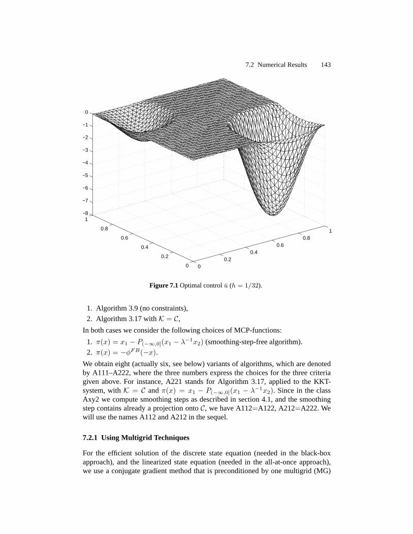
7.2 NumericalResults 143
00.2
0.40.6
0.81
0
0.2
0.4
0.6
0.8
1−8
−7
−6
−5
−4
−3
−2
−1
0
Figure7.1Optimalcontrol u (h = 1/32).
1. Algorithm 3.9(noconstraints),
2. Algorithm 3.17with K = C,In bothcasesweconsiderthefollowing choicesof MCP-functions:
1. π(x) = x1 − P(−∞,0](x1 − λ−1x2) (smoothing-step-freealgorithm).
2. π(x) = −φFB(−x).We obtaineight (actuallysix, seebelow) variantsof algorithms,which aredenotedby A111–A222,wherethe threenumbersexpressthe choicesfor the threecriteriagiven above. For instance,A221 standsfor Algorithm 3.17, appliedto the KKT-system,with K = C andπ(x) = x1 − P(−∞,0](x1 − λ−1x2). Sincein the classAxy2 we computesmoothingstepsasdescribedin section4.1, andthe smoothingstepcontainsalreadya projectionontoC, we have A112=A122, A212=A222.Wewill usethenamesA112andA212 in thesequel.
7.2.1 Using Multigrid Techniques
For the efficient solution of the discretestateequation(neededin the black-boxapproach),and the linearizedstateequation(neededin the all-at-onceapproach),we usea conjugategradientmethodthat is preconditionedby onemultigrid (MG)

144 7. Applications
00.2
0.40.6
0.81
0
0.2
0.4
0.6
0.8
1−0.12
−0.1
−0.08
−0.06
−0.04
−0.02
0
Figure7.2Optimalstatey(u) (h = 1/32).
V-cycle with one red-blackGauß-Seideliterationas presmootherandoneadjointred-blackGauß-Seideliterationaspostsmoother. Standardreferenceson multigridmethodsinclude [23, 72, 73, 145]. Our semismoothNewton methodswith MG-preconditionedconjugategradientsolver of theNewton systemsbelongto theclassof Newton multilevel methods[44]. For othermultigrid approachesto variationalinequalitieswereferto [21, 82, 83, 99, 100, 101].
For thesolutionof thesemismoothNewton systemwe solve theSchurcomple-mentequation(7.34) by a multigrid-preconditionedconjugategradientmethodasjust described.
The grid hierarchyis generatedas follows: The coarsesttriangulationT 1 isshown in Figure7.3. GivenT 2h, thenext finer triangulationT h is obtainedby re-placingany trianglein T 2h with four triangles,introducingthe edgemidpointsofthecoarsetrianglesasnew vertices,seeFigure7.4,which displaysT 1/2. Table7.1shows theresultingnumberof interior verticesandthenumberof trianglesfor eachtriangulationlevel. Thereis a secondstrategy to usethemultilevel philosophy:Wecanperforma nestediterationover the discretecontrol problemson the grid hier-archy:We first (approximately)solve the discretecontrol problemon the coarsestlevel. We theninterpolatethis solutionto obtainaninitial point for thediscretecon-

7.2 NumericalResults 145
Figure7.3CoarsesttriangulationT 1. Figure7.4SecondtriangulationT 1/2.
Numberof Numberofh interior vertices triangles
1/16 481 10241/32 1985 40961/64 8065 163841/128 32513 655361/256 130561 262144
Table 7.1Degreesof Freedomfor differentmeshsizes.
trol problemon the next finer level, which we againsolve approximately, andsoforth. As wewill see,this approachis veryefficient.
7.2.2 Black-Box Approach
We now presentnumericalresultsfor semismoothNewton methodsappliedto thefirst-ordernecessaryconditionsof thereducedproblem(7.9).We thusconsiderthethreealgorithmsA111, A121 andA112. The initial point is u0 ≡ −1. We do notusea globalizationsince(asit is oftenthecasefor controlproblems)theundampedsemismoothNewtonmethodconvergeswithoutdifficulties.Westressthatif thenon-monotonetrust-region methodof section6.4 is used,the globalizationparameterscanbechosenin sucha way thatthemethodessentiallybehaveslike thepureNew-ton method.
To beindependentof thechoiceof theMCP-function,we work with the termi-nationcondition
χ(uk) = ‖uk − PC(uk − j′(uk))‖L2 ≤ ε,or, in termsof thediscretizedproblem,[
uhk − PC(uhk − jhk′)]T
Mh[uhk − PC(uhk − jhk
′)]≤ ε2.

146 7. Applications
h k ‖uk − u‖L2 ‖uk − u‖L∞ χ(uk)
0 1.623e+00 6.416e+00 4.794e−031 9.454e−02 1.099e+00 1.022e−041
16 2 5.958e−04 1.354e−02 5.949e−043 3.611e−10 1.824e−09 3.552e−130 1.627e+00 6.477e+00 4.805e−031 9.191e−02 1.098e+00 9.934e−051
32 2 1.429e−03 5.833e−02 1.428e−033 8.267e−11 4.141e−10 7.712e−140 1.628e+00 6.482e+00 4.807e−031 9.052e−02 1.097e+00 9.769e−051
64 2 1.347e−03 5.959e−02 1.346e−033 6.616e−11 4.170e−10 1.254e−140 1.628e+00 6.487e+00 4.808e−031 9.019e−02 1.098e+00 9.732e−051
1282 1.247e−03 6.325e−02 1.246e−033 3.911e−08 1.001e−05 3.911e−084 7.098e−11 4.621e−10 1.285e−150 1.628e+00 6.488e+00 4.808e−031 8.988e−02 1.098e+00 9.697e−051
2562 1.309e−03 6.469e−02 1.308e−033 1.735e−07 8.885e−05 1.735e−074 8.935e−12 6.650e−11 1.450e−15
Table 7.2 Iterationhistoryof algorithmA111.
Exceptfrom this, the methodwe useagreeswith Algorithm 7.19. We work withε = 10−8. Smallervaluescanbechosenaswell, but it doesnot appearto beveryreasonableto chooseεmuchsmallerthanthediscretizationerror. Thenonlinearstateequationis solvedby a Newton iteration,where,in eachiteration,a linearizedstateequationhasto besolved.For thecomputationof j′ we solve theadjointequation.All PDEsolvesaredoneby amultigrid-cgmethodasdescribedabove.
In our first set of testswe chooseλ = 0.001 and considerproblemson thetriangulationsT h for h = 2−k, k = 4, 5, 6, 7, 8. SeeTable7.1for thecorrespondingnumberof trianglesandinterior nodes,respectively.
Theresultsarecollectedin Tables7.2–7.4.Hereby, Table7.2containstheresultsfor A111,Table7.3 theresultsfor A121,andTable7.4 theresultsfor A112.Listedaretheiterationk, theL2-distanceto the(discrete)solution(‖uk − u‖L2), theL∞-distanceto the(discrete)solution(‖uk − u‖L∞), andthenormof theprojectedgra-dient(χ(uk)). For all threevariantsof thealgorithmwe observe mesh-independentconvergencebehavior, andsuperlinearrateof convergenceof order>1. Only 3–4iterationsareneededuntil termination.
Table7.5 shows for all threealgorithmsthetotal numberof iterations(Iter.), ofstateequationsolves(State),of linearizedstateequationsolves(Lin. State),andofadjoint equationsolves(Adj. State),andthe total solutiontime in seconds(Time).The total numberof solvesof the semismoothNewton systemcoincideswith thenumberof iterationsIter. All solvesof the linearizedstateequationsareperformed

7.2 NumericalResults 147
h k ‖uk − u‖L2 ‖uk − u‖L∞ χ(uk)
0 1.623e+00 6.416e+00 4.794e−031 9.454e−02 1.099e+00 1.022e−041
16 2 3.266e−05 1.309e−04 5.467e−083 2.210e−10 1.115e−09 4.921e−140 1.627e+00 6.477e+00 4.805e−031 9.191e−02 1.098e+00 9.934e−051
32 2 5.613e−05 2.547e−04 9.082e−083 5.024e−11 2.521e−10 1.086e−140 1.628e+00 6.482e+00 4.807e−031 9.052e−02 1.097e+00 9.769e−051
64 2 5.348e−05 2.404e−04 8.643e−083 6.774e−11 4.115e−10 2.206e−150 1.628e+00 6.487e+00 4.808e−031 9.019e−02 1.098e+00 9.732e−051
128 2 4.679e−05 2.091e−04 7.538e−083 7.116e−11 4.612e−10 8.230e−160 1.628e+00 6.488e+00 4.808e−031 8.988e−02 1.098e+00 9.697e−051
256 2 5.097e−05 2.295e−04 8.212e−083 1.405e−07 6.736e−05 1.405e−10
Table 7.3 Iterationhistoryof algorithmA121.
within theNewtonmethodfor thesolutionof thestateequation.For algorithmsA111andA121,atotalof Iter+1 statesolvesandIter+1 adjointstatesolvesarerequired.Algorithm A112 requiresin additiononestatesolvesandoneadjointstatesolveperiterationfor thecomputationof thesmoothingstep.Weseethatusuallytwo Newtoniterationsaresufficient to solve the nonlinearstateequation.Observe that the totalcomputingtime increasesapproximatelylinearly with thedegreesof freedom.Thisshows that we indeedachieve multigrid efficiency. We note that algorithmsA111andA121 aresuperiorto A112 in computingtime. Themainreasonfor this is thatA112requirestheextrastateequationandadjointequationsolvesfor thesmoothingstep.
In a secondtestwe focuson theimportanceof thesmoothingstep.To this end,wehaveruntheAlgorithmsA112andA122withoutsmoothingsteps(A112is with-out projectionwhereasA122 containsa projection).Theresultsareshown in Table7.6. We seethat A112 without smoothingstepsneedsan averageof 7 iterations,whereastheregularAlgorithm A112,seeTable7.5,needsonly 4 iterationsin aver-age.This shows that thesmoothingstephasindeedbenefits,but that thealgorithmstill exhibits reasonableefficiency if the smoothingstepis removed. If we do notperforma smoothingstep,but includea projection(A122 without smoothingstep),theperformanceof thealgorithmis not affectedby omitting thesmoothingstep,atleastfor the problemunderconsideration.We recall that the role of thesmoothingstepis to avoid large discrepanciesbetween‖uk − u‖Lp and‖uk − u‖Lr , i.e., toavoid large (peak-like) deviationsof uk from u on smallsets,seeExample3.52.It

148 7. Applications
h k ‖uk − u‖L2 ‖uk − u‖L∞ χ(uk)
0 1.623e+00 6.416e+00 4.794e−031 6.695e−01 2.447e+00 1.630e−031
162 8.454e−02 3.252e−01 1.463e−043 9.587e−04 3.444e−03 1.601e−064 1.841e−09 6.849e−09 3.216e−120 1.627e+00 6.477e+00 4.805e−031 6.713e−01 2.466e+00 1.667e−031
322 9.340e−02 3.645e−01 1.654e−043 1.845e−03 7.274e−03 3.068e−064 1.540e−07 6.725e−07 2.516e−100 1.628e+00 6.482e+00 4.807e−031 6.718e−01 2.479e+00 1.682e−031
642 9.462e−02 3.731e−01 1.673e−043 1.737e−03 7.040e−03 2.891e−064 2.760e−07 1.316e−06 4.394e−100 1.628e+00 6.487e+00 4.808e−031 6.719e−01 2.483e+00 1.687e−031
1282 9.502e−02 3.794e−01 1.682e−043 1.773e−03 7.063e−03 2.959e−064 4.496e−07 1.930e−06 7.355e−100 1.628e+00 6.488e+00 4.808e−031 6.719e−01 2.485e+00 1.688e−031
2562 9.503e−02 3.796e−01 1.682e−043 1.770e−03 7.067e−03 2.954e−064 6.020e−07 2.442e−06 9.997e−10
Table 7.4 Iterationhistoryof algorithmA112.
is intuitively clearthataprojectionstepcanhelpin cuttingoff suchpeaks(but thereis noguarantee).
In our next test we show that lack of strict complementaritydoesnot affectthe superlinearconvergenceof the algorithms.Denotingby j the reducedobjec-tivefunctionfor thedata(7.35)andby u thecorrespondingsolution,wenow chooseud = λ−1j′(u). With thesenew data,the(new) gradientvanishesidenticallyonΩat u so that strict complementarityis violated.A representative run for this degen-eratedproblemis shown in Table7.7(A111,h = 1/128). Hereby, uhd wasobtainedfrom thediscretesolutionandthediscretegradient.Similar asin thenondegeneratecase,the algorithmsshow meshindependentbehavior, seeTable7.8. We have notincludedfurthertablesfor this problemsincethey would look essentiallylike thosefor thenondegenerateproblem.
7.2.3 All-at-Once Approach
Wenow presentnumericalexperimentsfor semismoothNewtonmethodsappliedtotheall-at-onceapproach.Sincethestateequationis nonlinear, theadvantageof thisapproachis that we do not have to solve the stateequationin every iteration.On

7.2 NumericalResults 149
Alg. h Iter. State Lin. State Adj. State Time1/16 3 4 10 4 3.0s1/32 3 4 9 4 8.6s
A111 1/64 3 4 7 4 32.6s1/128 4 5 8 5 187.8s1/256 4 5 8 5 935.5s1/16 3 4 9 4 2.9s1/32 3 4 8 4 8.2s
A121 1/64 3 4 7 4 33.0s1/128 3 4 7 4 156.8s1/256 3 4 7 4 771.1s1/16 4 9 21 9 6.0s1/32 4 9 19 9 16.0s
A112 1/64 4 9 19 9 65.3s1/128 4 9 19 9 300.7s1/256 4 9 18 9 1428.1s
Table 7.5Performancesummaryfor thealgorithmsA111,A121,andA112.
h Iter. State Lin. State Adj. State TimeAlgorithm A112without smoothingstep
1/16 7 8 16 8 6.2s1/32 7 8 15 8 18.4s1/64 7 8 15 8 76.7s1/128 7 8 15 8 366.2s1/256 7 8 14 8 1834.2s
Algorithm A122without smoothingstep.1/16 4 5 13 5 4.5s1/32 4 5 11 5 11.2s1/64 4 5 11 5 50.0s1/128 4 5 11 5 263.6s1/256 4 5 10 5 1191.8s
Table 7.6Performancesummaryfor algorithmsA112andA122withoutsmoothingstep.
the otherhand,the mainwork is solving the Newton systemso that an increaseofiterationsin thesemismoothNewtonmethodcancompensatethis win of time.
Wechooseu0 ≡ −1, y0 ≡ 0, w0 ≡ 0. Betterchoicesfor y0 andw0 arecertainlypossible.Our terminationconditionis
χ(yk, uk, wk) =(‖Lu(yk, uk, wk)− PC(uk − Lu(yk, uk, wk))‖2L2
+ ‖Ly(yk, uk, wk)‖2H−1 + ‖E(yk, uk)‖2H−1
)1/2 ≤ εwith ε = 10−8. Theall-at-oncesemismoothNewtonsystemis solvedby reducingitto thesameSchurcomplementaswasusedfor solvingtheblack-boxNewtonequa-tion, andby applyingMG-preconditionedcg. Only the right handsideis different.Table7.9showstwo representativerunsof algorithmA212.Furthermore,Table7.10

150 7. Applications
h k ‖uk − u‖L2 ‖uk − u‖L∞ χ(uk)
0 1.628e+00 6.487e+00 2.053e-031 9.019e-02 1.098e+00 1.006e-041
128 2 1.657e-07 4.789e-07 1.536e-073 8.814e-12 2.260e-11 1.738e-17
Table 7.7 Iterationhistoryof algorithmA111 for adegenerateproblem.
h Iter. State Lin. State Adj. State Time1/16 3 4 9 4 2.7s1/32 3 4 9 4 7.9s1/64 3 4 7 4 32.7s1/128 3 4 7 4 157.6s1/256 3 4 7 4 767.1s
Table 7.8Performancesummaryof algorithmA111 for adegenerateproblem.
h k ‖uk − u‖L2 ‖uk − u‖L∞ χ(yk, uk, wk)
0 1.628e+00 6.487e+00 1.903e-011 6.797e-01 2.514e+00 3.225e-012 1.176e-01 4.743e-01 4.007e-021
128 3 3.025e-03 1.197e-02 1.068e-034 1.756e-06 6.915e-06 6.767e-075 3.000e-13 1.206e-12 8.823e-110 1.628e+00 6.488e+00 1.903e-011 6.797e-01 2.516e+00 3.225e-012 1.156e-01 4.645e-01 3.949e-021
256 3 2.935e-03 1.171e-02 1.041e-034 2.079e-06 8.583e-06 7.832e-075 6.203e-14 2.888e-13 5.604e-11
Table 7.9 Iterationhistoryof algorithmA212.
containsinformationon theperformanceof thealgorithmsA211, A221, andA212for differentmeshsizes.
In comparisonwith the black-boxalgorithms,we seethat all-at-onceapproachandblack-boxapproacharecomparablyefficient.As anadvantageof theall-at-onceapproachwe note that the smoothingstepcanbe performedwith minimum addi-tional cost,whereasin the black-boxapproachit requiresoneadditionalsolve ofboth,stateandandadjointequation.Webelievethatthemoreexpensiveto solvethestateequationis (dueto nonlinearity),themorefavorableis theall-at-onceapproach.
7.2.4 NestedIteration
Next, we presentnumericalresultsfor the nestediteration approach.Hereby, westarton thegrid T 1/2, solve theproblemwith terminationthresholdε = 10−5 andcomputefrom its solution an initial point for the problemon the next finer grid

7.2 NumericalResults 151
Algorithmh A211 A221 A212
Iter. Time Iter. Time Iter. Time1/16 5 1.9s 5 1.9s 5 2.4s1/32 5 6.1s 5 6.1s 5 6.7s1/64 5 28.0s 5 27.9s 5 30.3s1/128 5 147.2s 5 147.1s 5 156.3s1/256 5 750.9s 5 752.5s 5 785.0s
Table 7.10Performancesummaryfor thealgorithmsA211,A221,andA212.
T 1/4, andsoon.On thefinestlevel we solve with terminationthresholdε = 10−8.Table 7.11 shows the numberof iterationsper level and the total executiontime
Lin. Adj. Lin. Adj.h Iter. State State State h Iter. State State State
1/2 1 2 6 2 1/32 2 3 6 31/4 2 3 7 3 1/64 1 2 4 21/8 2 3 6 3 1/128 1 2 4 21/16 2 3 6 3 1/256 1 2 4 2
Total Time: 360s
Table 7.11Performancesummaryfor nestediterationversionof algorithmA111.
for the nestedversionof algorithmA111. Comparisonwith Table7.11shows thatthenestedversionof A111 needslessthanhalf the time to solve the problemthantheunnestedversion(330vs. 935seconds).Theuseof nestediterationis thusverypromising.Furthermore,it is very robustsince,exceptfor thecoarsestproblem,theNewton iterationis startedwith a verygoodinitial point.
7.2.5 Discussionof the Results
Fromthepresentednumericalresultswe draw thefollowing conclusions:
• The proposedmethodsallow us to usefast iterative solvers for their imple-mentation.This leadsto runtimesof optimal order in the sensethat they areapproximatelyproportionalto thenumberof unknowns.
• Theclassof semismoothNewtonmethodsperformsveryefficiently andexhibitsmesh-independentbehavior. We observe superlinearconvergenceaspredictedby our theory.
• Both,black-boxandall-at-onceapproachleadto efficientandrobustalgorithmswhich arecomparablein runtime.If smoothingstepsareused,the all-at-onceapproachis advantageoussinceit doesnot requireadditionalstateandadjointstatesolvesto computethesmoothingstep.

152 7. Applications
• Lack of strict complementaritydoesnotaffect thefastconvergenceof thealgo-rithms.Thisconfirmsour theory, whichdoesnotrequirestrictcomplementarity.
• Thechoiceof theMCP-functionπ(x) = x1 − PC(x1 − λ−1x2) appearsto bepreferabletoπ(x) = −φFB(−x) for thisclassof problems,atleastin theblack-box-approach.Themainreasonfor this is theadditionalcostof thesmoothingstep.
• Theperformanceof theφFB-basedalgorithms,which from a theoreticalpointof view requireasmoothingstep,degradesby acertainmargin if thesmoothingstepis turnedoff. This, however, is compensatedif we turn on the projectionstep.Our numericalexperienceindicatesthat this effect is problemdependent.It shouldbementionedthat so far we never observeda severedeteriorationofperformancewhenswitchingoff thesmoothingstep.But we stressthatpatho-logical situationslike theonein Example3.52canoccur, andthatthey resultina stagnationof convergenceonfine grids(we havetried this,but donot includenumericalresultshere).
Weconcludethissectionby notingthatmany othercontrolproblemscanbehandledin a similar way. In particular, Neumannboundarycontrol canbe usedinsteadofdistributedcontrol.Furthermore,thecontrolof othertypesof PDEsby semismoothNewton methodsis possible,e.g.,Neumannboundarycontrolof thewave equation[104] andNeumannboundarycontrol of the heatequation[24, 143]. The optimalcontrolof theincompressibleNavier–Stokesequationsis consideredin section8.
7.3 ObstacleProblems
In this sectionwe studythe classof obstacleproblemsdescribedin section1.1.2.Obstacleproblemsof this or similar typearisein many applications,e.g.,potentialflow of perfectfluids, lubrication,wake problems,etc.,see,e.g.,[63] andthe ref-erencestherein.We describethe problemin termsof the obstacleproblemfor anelasticmembrane.
For q ∈ [2,∞), let g ∈ H2,q(Ω) representa (lower) obstaclelocatedover thenonemptyboundedopensetΩ ⊂ R2 with sufficiently smoothboundary, denotebyy ∈ H1
0 (Ω) the positionof a membrane,andby f ∈ Lq(Ω) external forces.Forcompatibilitywe assumeg ≤ 0 on∂Ω, which is assumedto besufficiently smooth.Theny ∈ H1
0 (Ω) solvesthevariationalinequality
y ≥ g on Ω,
a(y, v − y)− (f, v − y)L2 ≥ 0 ∀ v ∈ H10 (Ω), v ≥ g on Ω,
(7.36)
where
a : H10 (Ω)×H1
0 (Ω)→ R, a(y, z) =∑i,j
aij∂y
∂xi
∂z
∂xj,
aij = aji ∈ C1(Ω), anda beingH10 -elliptic, i.e.,

7.3 ObstacleProblems 153
a(y, y) ≥ ν‖y‖2H10∀y ∈ H1
0 (Ω)
with a constantν > 0. Theboundedbilinear form a inducesa boundedlinearop-eratorA ∈ L(H1
0 ,H−1) via a(v,w) = 〈v,Aw〉H1
0 ,H−1 for all v,w ∈ H1
0 (Ω).The ellipticity of a and the Lax–Milgram theoremimply thatA ∈ L(H1
0 ,H−1)
is a homeomorphismwith ‖A−1‖H−1,H10≤ ν−1, andregularity resultsimply that
A−1 ∈ L(L2,H2).Introducingtheclosedconvex set
F = y ∈ H10 (Ω) : y ≥ g on Ω
andtheobjective functionJ : H10 (Ω) 7→ R,
J(y) def=12a(y, y)− (f, y)L2 ,
wecanwrite (7.36)equivalentlyasoptimizationproblem
minimize J(y) subjectto y ∈ F . (7.37)
Theellipticity of a impliesthatJ is strictly convex with J(y)→∞ as‖y‖H10→∞.
Hence,using that F is a closedand convex subsetof the Hilbert spaceH10 (Ω),
we seethat (7.37) possessesa uniquesolution y ∈ F [49, Prop. II.1.2]. Further,regularity results[22, Thm.I.1] ensurethat y ∈ H1
0 (Ω) ∩H2,q(Ω).
7.3.1 Dual Problem
Since(7.37) is not posedin anLp-setting,we derive an equivalentdual problem,which,aswe will see,is posedin L2(Ω). Denotingby IF : H1
0 (Ω)→ R ∪ +∞,theindicatorfunctionof F , i.e.,IF (y)(x) = 0 for x ∈ F andIF(y)(x) = +∞ forx /∈ F , we canwrite (7.37)in theform
infy∈H1
0 (Ω)J(y) + IF (y). (7.38)
The corresponding(Fenchel–Rockafellar)dual problem[49, Ch. III.4] (we chooseF = IF ,G = J , Λ = I, u = y, andp∗ = −u in theterminologyof [49]) is
supu∈H−1(Ω)
−J∗(u)− I∗F (−u), (7.39)
whereJ∗ : H−1(Ω) → R ∪ +∞ andI∗F : H−1(Ω) → R ∪ +∞ are theconjugatefunctionsof F andIF , respectively:
J∗(u) = supy∈H1
0 (Ω)
〈y, u〉H10 ,H
−1 − J(u), (7.40)
I∗F (u) = supy∈H1
0 (Ω)
〈y, u〉H10 ,H
−1 − IF (y). (7.41)
(7.42)

154 7. Applications
Let y0 ∈ H10 (Ω) be suchthat IF (y0) = 0, e.g.,y0 = y. ThenJ is continuous
at y0 andIF is boundedat y0. Furthermore,sinceIF ≥ 0, the ellipticity impliesJ(y) + IF (y) → ∞ as‖y‖H1
0→ ∞. Therefore,[49, Thm. III.4.2] appliesso that
(7.38)and(7.39)possesssolutionsy (thisweknew already)andu, respectively, andfor any pair of solutionsholds
J(y) + IF (y) + J∗(u) + I∗F (−u) = 0.
Further, thefollowing extremalityrelationshold:
J(y) + J∗(u)− 〈u, y〉H−1,H10
= 0, (7.43)
IF (y) + I∗F (−u) + 〈u, y〉H−1,H10
= 0. (7.44)
This implies
u ∈ ∂J(y), (7.45)
−u ∈ ∂IF (y). (7.46)
In our caseJ is smooth,whichyields
u = J ′(y) = Ay − f. (7.47)
Weknow thattheprimalsolutiony is unique,andthusthedualsolutionu is unique,too, by (7.47). Further, by regularity, y ∈ H1
0 (Ω) ∩ H2,q(Ω), which, via (7.47),impliesu ∈ Lq(Ω).
Thesupremumin thedefinitionof J∗, see(7.40),is attainedfor y = A−1(f+u),with value
J∗(u) = 〈u, y〉H−1,H10− 1
2〈y,Ay〉H1
0 ,H−1 + 〈f, y〉H−1,H1
0
=12〈f + u,A−1(f + u)〉H−1,H1
0.
For u ∈ L2(Ω) we canwrite
J∗(u) =12(f + u,A−1(f + u))L2 .
Further, seealso[22, p. 19] and[49, Ch. IV.4],
I∗F (u) = supy∈H1
0
〈u, y〉H−1,H10− IF (y) = sup
y∈F〈u, y〉H−1,H1
0.
For u ∈ L2(Ω) we have
I∗F (u) = supy∈F
(u, y)L2 =
(g, u)L2 if u ≤ 0 onΩ,+∞ otherwise.
Therefore,usingtheregularityof y andu, wecanwrite (7.39)in theform

7.3 ObstacleProblems 155
maximizeu∈L2(Ω)
− 12(f + u,A−1(f + u))L2 + (g, u)L2 subjectto u ≥ 0, (7.48)
andweknow thatu ∈ Lq(Ω). Werecallthatfrom thedualsolutionuwecanrecovertheprimal solutiony from theidentity (7.47):y = A−1(f + u).
In thefollowing wepreferto write (7.48)asaminimizationproblem:
minimizeu∈L2(Ω)
12(f + u,A−1(f + u))L2 − (g, u)L2 subjectto u ≥ 0. (7.49)
Example7.21. In thecaseA = −∆ theprimal problemis
minimizey∈H1
0 (Ω)
12‖y‖2H1
0− (f, y)L2 subjectto y ≥ g,
andthedual(minimization)problemreads
minimizeu∈L2(Ω)
12‖f + u‖2H−1 − (g, u)L2 subjectto u ≥ 0,
where‖u‖H−1 = ‖∆−1u‖H10
is thenormdualto ‖ · ‖H10.
Wecollectour resultsin thefollowing theorem.
Theorem7.22. Under the problemassumptions,the obstacleproblem(7.36)pos-sessesa uniquesolutiony ∈ H1
0 (Ω), andthissolutionis containedinH2,q(Ω). Thedual problem(7.39)possessesa uniquesolutionu ∈ H−1(Ω) aswell. Primal anddual solutionare linkedvia theequation
Ay = f + u.
In particular, u ∈ Lq(Ω), andthedual (minimization)problemcanbewritten in theform (7.49).
7.3.2 RegularizedDual Problem
Problem(7.49)is not coercive in thesensethatfor ‖u‖L2 → ∞ theobjective func-tion tendsto +∞. Hence,we considertheregularizedproblem
minimizeu∈L2(Ω)
jλ(u)def=
12(f + u,A−1(f + u))L2 +
λ
2‖u− ud‖2L2 − (g, u)L2
subjectto u ≥ 0 on Ω
(7.50)
with ud ∈ Lp′(Ω), p′ ∈ (2,∞), and(small) regularizationparameterλ > 0. Thisproblemhasthefollowing properties:

156 7. Applications
Theorem7.23. Theobjectivefunctionof problem(7.50)is stronglyconvex and
jλ(u)→∞ as‖u‖L2 →∞.In particular, (7.50)possessesa uniquesolutionuλ ∈ L2(Ω), andthis solutionliesin Lp
′(Ω). Thederivativeof jλ hastheform
j′λ(u) = λ(u− ud) + A−1(f + u)− g def= λu+G(u). (7.51)
Hereby, themappingG(u) = A−1(f +u)− g−λud mapsL2(Ω) continuouslyandaffinelinearly intoLp
′(Ω).
Proof. Obviously, jλ is asmoothquadraticfunctionandwith z = A−1(f + u),
jλ(u) =λ
2‖u− ud‖2L2 +
12a(z, z) − (g, u)L2
≥ λ
2‖u− ud‖2L2 − ‖g‖L2‖u‖L2 →∞
as‖u‖L2 → ∞. Therefore,sinceu ∈ L2(Ω) : u ≥ 0 is closedandconvex, weseethat(7.50)possessesauniquesolutionuλ ∈ L2(Ω).
Certainly, j′λ(u) is givenby (7.51),andthe fact thatA ∈ L(H10 ,H
−1) impliesthat
G : u ∈ L2(Ω) 7→ A−1(f + u)− g − λud ∈ H10 (Ω) + Lp
′(Ω) → Lp
′(Ω)
is continuousaffine linear. Fromtheoptimalityconditionsfor (7.50)we conclude
j′λ(uλ) = 0 on x ∈ Ω : uλ(x) 6= 0.Hence,
uλ = 1uλ 6=0uλ = −λ−11uλ 6=0G(uλ) ∈ Lp′(Ω).
utCorollary 7.24. Undertheproblemassumptions,F = j′λ satisfiesAssumption3.33(a), (b) for anyp ∈ [2,∞), anyp′ ∈ [2,∞) with p′ ≤ p andud ∈ Lp′(Ω), andany1 ≤ r < p′. Furthermore, F satisfiesAssumption4.1 for r = 2 andall p ∈ (2,∞)with ud ∈ Lp(Ω). Finally, F alsosatisfiesAssumption4.6(a)–(e) for all p ∈ [2,∞)andall p′ ∈ (2,∞).
Proof. The Corollary is an immediateconsequenceof Theorem7.23 and theL2-coercivity of jλ. utRemark 7.25. Corollary7.24establishesall assumptionsthatareneededto estab-lish the semismoothnessof NCP-functionbasedreformulations.In fact, for gen-eral NCP-functionsTheorem3.45 is applicable,whereasfor the special choiceπ(x) = x1 − P[0,∞)(x1 − λ−1x2) we canuseTheorem4.4.Furthermore,thesuffi-cientconditionfor regularityof Theorem4.8is applicable.Hence,wecanapplyourclassof semismoothNewtonmethodsto solveproblem(7.50).

7.3 ObstacleProblems 157
Next, wederiveboundsfor theapproximationerrors‖uλ− u‖H−1 and‖yλ− y‖H10,
whereyλ = A−1(f + uλ).
Theorem7.26. Let u anduλ denotethesolutionsof (7.49)and(7.50), respectively.Theny = A−1(f+u) solvestheobstacleproblem(7.36)andwith yλ = A−1(f+uλ)holds,asλ→ 0+ :
‖uλ − u‖H−1 = o(λ1/2), (7.52)
‖yλ − y‖H10
= o(λ1/2). (7.53)
Proof. By Theorems7.22and7.23we know that the dual problem(7.49)andtheregularizeddualproblem(7.50)possessuniquesolutionsu, uλ ∈ Lp(Ω). Now
jλ(uλ) ≤ jλ(u) = j(u) +λ
2‖u− ud‖2L2 ≤ j(uλ) +
λ
2‖u− ud‖2L2
= jλ(uλ) +λ
2(‖u− ud‖2L2 − ‖uλ − ud‖2L2
).
Thisproves‖uλ − ud‖L2 ≤ ‖u− ud‖L2 . (7.54)
Further,
j(u) ≤ j(uλ) = jλ(uλ)− λ
2‖uλ − ud‖2L2 ≤ jλ(u)− λ
2‖uλ − ud‖2L2
= j(u) +λ
2(‖u− ud‖2L2 − ‖uλ − ud‖2L2
) ≤ j(u) +λ
2‖u− ud‖2L2 .
(7.55)
Therefore,
0 ≤ j(uλ)− j(u) ≤ λ
2‖u− ud‖2L2 = O(λ) as λ→ 0+.
Now let λk → 0+. Since
M = u ∈ L2(Ω) : u ≥ 0, ‖u− ud‖L2 ≤ ‖u− ud‖L2is closed,convex, andbounded,thereexistsa subsequenceandapoint u ∈ M suchthatuλk′ → u weakly in L2. Sincej is convex andcontinuous,it is weakly lowersemicontinuous,sothat
j(u) ≤ j(u) ≤ lim infk′→∞
j(uλk′ ) = lim infk′→∞
[j(u) +O(λk′)
]= j(u).
Henceu is a solutionof (7.49)andthereforeu = u, sinceu is theuniquesolution.By a subsequence-subsequenceargumentwe conclude
uλ → u weaklyin L2(Ω) as λ→ 0+. (7.56)
Sinceu 7→ ‖u − ud‖L2 is convex andcontinuous,henceweakly lower semicontin-uous,we obtainfrom (7.54)and(7.56)

158 7. Applications
‖u− ud‖L2 ≤ lim infλ→0+
‖uλ − ud‖L2 ,
‖u− ud‖L2 ≥ lim supλ→0+
‖uλ − ud‖L2 ,
whichproves‖uλ − ud‖L2 → ‖u− ud‖L2 as λ→ 0+. (7.57)
SinceL2 is aHilbert space,(7.56)and(7.57)imply
uλ → u in L2 as λ→ 0+. (7.58)
Hence,(7.55)impliesj(uλ)− j(u) = o(λ).
Sinceu solves(7.49),thereholds(j′(u), uλ − u)L2 ≥ 0. Therefore,
j(uλ)− j(u) = (j′(u), uλ − u)L2 +12(uλ − u, j′′(u)(uλ − u))L2
≥ 12(uλ − u, j′′(u)(uλ − u))L2 =
12(uλ − u, A−1(uλ − u))L2 .
Hence,with v = uλ − u andw = A−1v,
‖v‖2H−1 = ‖Aw‖2H−1 ≤ ‖A‖2H10 ,H
−1‖w‖2H10≤ ‖A‖2H1
0 ,H−1κ
−1〈w,Aw〉H10 ,H
−1
≤ κ−1‖A‖2H10 ,H
−1〈v,w〉L2 ≤ 2κ−1‖A‖2H10 ,H
−1(j(uλ)− j(u))= 2κ−1‖A‖2H1
0 ,H−1o(λ).
This proves(7.52).The solutionof the obstacleproblemis y = A−1(f + u). Foryλ = A−1(f + uλ) holds:
‖yλ − y‖2H10
= ‖A−1(uλ − u)‖2H10
= ‖w‖2H10≤ κ−1〈w,Aw〉H1
0 ,H−1
= κ−1(uλ − u, A−1(uλ − u))L2 ≤ 2κ−1(j(uλ)− j(u))= 2κ−1o(λ).
Theproof is complete. utRemark 7.27. Theparameterλ hasto bechosensufficiently smallto ensurethattheerroris not largerthanthediscretizationerror. Our approachwill beto successivelyreduceλ.
7.3.3 Discretization
We usethe samefinite elementspacesas in section7.1.3.A straightforward dis-cretizationyieldsthediscreteobstacleproblem(in coordinateform)
minimizeyh∈Rnh
12yh
TAhyh − fh
Tyh subjectto yh ≥ gh. (7.59)

7.3 ObstacleProblems 159
Hereby, gh ∈ Rnh
, ghi = g(P hi ), approximatesthe obstacle.Furthermore,fhi =(βhi , f)L2 , andAh
ij = (Aβhi , βhj )H−1,H1
0. Thecorrespondingdualproblemis
minimizeuh∈Rnh
12(fh + Shuh)TAh−1
(fh + Shuh)− ghTShuh
subjectto uh ≥ 0.(7.60)
Hereby, Sh ∈ Rnh×nh
is definedasin (7.17).Thediscreteregularizeddualproblemthenis givenby
minimizeuh∈Rnh jhλ(u
h) def=12(fh + Shuh)TAh−1
(fh + Shuh)
+λ
2(uh − uhd)
TSh(uh − uhd)− ghTShuh
subjectto uh ≥ 0,
(7.61)
where,e.g.,[Shuhd ]i = (Lhβhi , Lhud)L2 . Fromthesolutionuhλ of (7.61)wecompute
yhλ via Ahyhλ = fh + Shuhλ.Thegradientof jhλ
′andtheHessianjhλ
′′of jhλ with respectto theSh-innerproduct
aregivenby
jhλ′(uh) = Ah−1
(fh + Shuh) + λ(uh − uhd)− gh,
jhλ′′(uh) = Ah−1
Sh + λI.
Choosinga LipschitzcontinuousandsemismoothNCP-functionφ, we reformulate(7.61)in theform
Φh(uh) def=
φ(uh1 , j
hλ
′(uh)1)
...φ(uhnh , jhλ
′(uh)nh
) = 0. (7.62)
This is thediscretecounterpartof thesemismoothreformulationin functionspace
Φ(u) def= φ(u, j′λ(u)
)= 0.
As in section 7.1.4, we can argue that an appropriatediscretizationof ∂Φ is∂Φh(uh), thesetof all matricesBh ∈ Rnh×nh
with
Bh = Dh1 + Dh
2 jhλ
′′(uh), (7.63)
whereDh1 andDh
2 arediagonalmatricessuchthat((Dh
1)ll, (Dh2 )ll) ∈ ∂φ(uhl , jhλ′(uh)l), l = 1, . . . , nh.
Again,we havetheinclusion

160 7. Applications
∂CΦh(uh) ⊂ ∂Φh(uh)
with equalityif φ or−φ is regular. With thesameargumentationasin thederivationof Theorem7.18we canshow thatΦh is ∂Φh-semismooth(andthusalsosemis-mooth in the usualsense).Semismoothnessof higherordercanbe proved analo-gously. Hence,we canapplyour semismoothNewton methodsto solve (7.62).Thedetailsof theresultingalgorithm,whicharenotgivenhere,parallelAlgorithm 7.62.The centraltaskis to solve the semismoothNewton system(we suppressthe sub-scriptk)
[Dh1 + Dh
2 jhλ
′′(uh)]sh = −Φh(uh).
Usingthestructureof jhλ′′
andthat(Dh1 + λDh
2) is diagonalandpositivedefinitefor
ourchoicesof φ, weseethatthis is equivalentto sh = Sh−1
Ahvh, wherevh solves
[Ah + Sh(Dh1 + λDh
2)−1Dh2 ]vh = −Sh(Dh
1 + λDh2)−1Φh(uh).
Thiscanbeviewedasadiscretizationof thethePDE
Av +d2
d1 + λd2v =
−1d1 + λd2
Φ(u).
Therefore,we canapplya multigrid methodto computevh, from which sh canbeobtainedeasily.
7.3.4 Numerical Results
Weconsiderthefollowing problem:
Ω = (0, 1)× (0, 1),
g = −14
+12
sin(πx1) sin(πx2)
f = −5 sin(2πx1) sin(2πx2)(
12
+ e2x1+x2
).
(7.64)
Thetriangulationis thesameasin section7.2.1.Again, thecodewasimplementedin MatlabVersion6 Release12,usingsparsematrix computations,andwasrun un-derSolaris8 onaSunSPARC Ultra workstationwith asparcv9processoroperatingat 360MHz. To obtainsufficiently accuratesolutions,the regularizationparameterhasto bechosenappropriately. Hereby, we usea nestediterationapproachandde-termineλ in dependenceon the currentmeshsize.It is known [63, App. I.3] that,underappropriateconditions,thedescribedfinite elementdiscretizationleadsto ap-proximationerrors‖yh− y‖H1
0= O(h). Sincewehaveshown in Theorem7.26that
‖yλ − y‖H10
= o(λ1/2), we chooseλ of theorderh2, moreprecisely, we work with
λ = λh =h2
10.
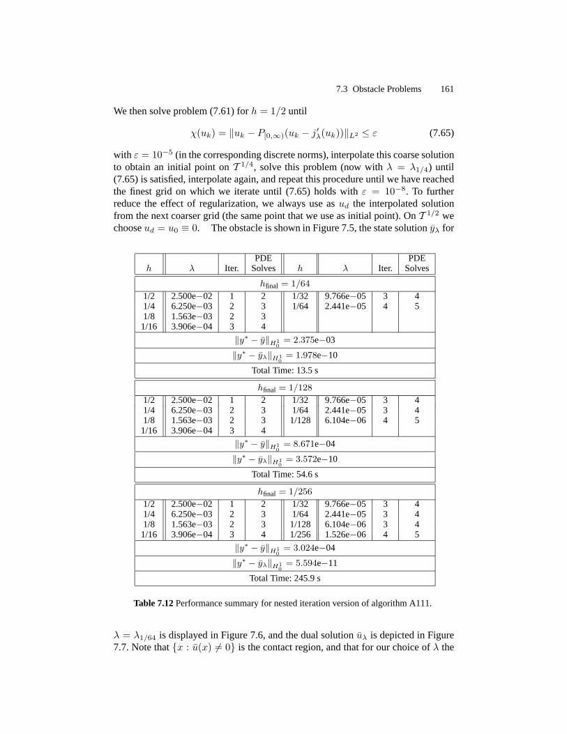
7.3 ObstacleProblems 161
Wethensolveproblem(7.61)for h = 1/2 until
χ(uk) = ‖uk − P[0,∞)(uk − j′λ(uk))‖L2 ≤ ε (7.65)
with ε = 10−5 (in thecorrespondingdiscretenorms),interpolatethiscoarsesolutionto obtainan initial point on T 1/4, solve this problem(now with λ = λ1/4) until(7.65)is satisfied,interpolateagain,andrepeatthisprocedureuntil wehavereachedthe finest grid on which we iterateuntil (7.65) holds with ε = 10−8. To furtherreducethe effect of regularization,we always useasud the interpolatedsolutionfrom thenext coarsergrid (thesamepoint thatwe useasinitial point).OnT 1/2 wechooseud = u0 ≡ 0. Theobstacleis shown in Figure7.5,thestatesolutionyλ for
PDE PDEh λ Iter. Solves h λ Iter. Solves
hfinal = 1/64
1/2 2.500e−02 1 2 1/32 9.766e−05 3 41/4 6.250e−03 2 3 1/64 2.441e−05 4 51/8 1.563e−03 2 31/16 3.906e−04 3 4
‖y∗ − y‖H10
= 2.375e−03
‖y∗ − yλ‖H10
= 1.978e−10
Total Time: 13.5s
hfinal = 1/128
1/2 2.500e−02 1 2 1/32 9.766e−05 3 41/4 6.250e−03 2 3 1/64 2.441e−05 3 41/8 1.563e−03 2 3 1/128 6.104e−06 4 51/16 3.906e−04 3 4
‖y∗ − y‖H10
= 8.671e−04
‖y∗ − yλ‖H10
= 3.572e−10
Total Time: 54.6s
hfinal = 1/256
1/2 2.500e−02 1 2 1/32 9.766e−05 3 41/4 6.250e−03 2 3 1/64 2.441e−05 3 41/8 1.563e−03 2 3 1/128 6.104e−06 3 41/16 3.906e−04 3 4 1/256 1.526e−06 4 5
‖y∗ − y‖H10
= 3.024e−04
‖y∗ − yλ‖H10
= 5.594e−11
Total Time: 245.9s
Table 7.12Performancesummaryfor nestediterationversionof algorithmA111.
λ = λ1/64 is displayedin Figure7.6,andthedualsolutionuλ is depictedin Figure7.7.Notethatx : u(x) 6= 0 is thecontactregion,andthat for our choiceof λ the

162 7. Applications
Algorithm A111
k ‖yk − yλ‖H10
‖yk − y‖H10
χ(uk)
0 1.701e-03 1.862e-03 5.812e-051 5.648e-04 6.199e-04 3.273e-012 2.682e-05 3.034e-04 1.706e-023 2.333e-09 3.024e-04 7.343e-074 5.594e-11 3.024e-04 8.139e-11
Table 7.13Iterationhistoryof algorithmA111on thefinal level h = hfinal = 1/256.
00.2
0.40.6
0.81
0
0.2
0.4
0.6
0.8
1−0.4
−0.2
0
0.2
0.4
0.6
Figure7.5Theobstacleg (h = 1/64).
solutionu is approximatedup to a fractionof thediscretizationerrorby uλ. It canbeseenthatu is discontinuousat theboundaryof thecontactregion.
In the numericaltestsit turnedout that it is not advantageousto let λ−1 be-cometoo large in the smoothingsteps.Hence,we set γ = min105, λ−1 andwork with smoothingstepsof the form Sk(u) = P[0,∞)(u − γj′λ(u)). On theother hand,even very small λ doesnot causeany problemsin the NCP-functionφ(x) = x1−P[0,∞)(x1−λ−1). Weconsidertwo methods:Thesmoothing-step-freeAlgorithm A111 with φ(x) = x1 − P[0,∞)(x1 − λ−1), andAlgorithm A112 withφFB andsmoothingstepasjustdescribed.It turnsout thatwithoutglobalizationthe

7.3 ObstacleProblems 163
PDE PDEh λ Iter. Solves h λ Iter. Solves
hfinal = 1/64
1/2 2.500e−02 4 9 1/32 9.766e−05 4 91/4 6.250e−03 3 7 1/64 2.441e−05 5 111/8 1.563e−03 4 91/16 3.906e−04 4 9
‖y∗ − y‖H10
= 2.374e−03
‖y∗ − yλ‖H10
= 1.631e−07
Total Time: 29.3s
hfinal = 1/128
1/2 2.500e−02 4 9 1/32 9.766e−05 4 91/4 6.250e−03 3 7 1/64 2.441e−05 4 91/8 1.563e−03 4 9 1/128 6.104e−06 6 131/16 3.906e−04 4 9
‖y∗ − y‖H10
= 8.670e−04
‖y∗ − yλ‖H10
= 3.069e−08
Total Time: 142.9s
hfinal = 1/256
1/2 2.500e−02 4 9 1/32 9.766e−05 4 91/4 6.250e−03 3 7 1/64 2.441e−05 4 91/8 1.563e−03 4 9 1/128 6.104e−06 4 91/16 3.906e−04 4 9 1/256 1.526e−06 5 11
‖y∗ − y‖H10
= 3.024e−04
‖y∗ − yλ‖H10
= 2.609e−11
Total Time: 613.9s
Table 7.14Performancesummaryfor nestediterationversionof algorithmA112.
projectedvariantA121 tendsto cycle whenλ becomesvery small.Sinceincorpo-ratingaglobalizationrequiresadditionalevaluationsof jλ and/orits gradient,whichis expensive dueto thepresenceof A−1, we do not presentnumericalresultsfor aglobalizedversionof A121.
In Table7.12(A111)andTable7.14(A112)weshow, for eachlevel of thenestediteration,thevalueof λ, thenumberof iterationsperformedon this level (Iter), andthenumberof PDEsolves.Furthermore,the(discrete)distance‖y∗ − y‖H1
0of the
(discrete)computedsolutiony∗ to the(discrete)solutiony correspondingto λ = 0andthe (discrete)distance‖y∗ − yλ‖H1
0of the (discrete)computedsolutiony∗ to
the (discrete)solutionyλ correspondingto λ = h2final/10 areshown. The total run-
time is alsogiven.We seethaton eachlevel only a few Newton iterationsareper-formed.In Table7.13the iterationhistoryof A111 on thefinestlevel is shown forhfinal = 1/256. Obviously, the convergenceis superlinearwith rate>1, and weobserve mesh-independentperformanceof the methods.Furthermore,the runtime

164 7. Applications
00.2
0.40.6
0.81
0
0.2
0.4
0.6
0.8
1−0.4
−0.2
0
0.2
0.4
0.6
Figure7.6Computedstateyλ (h = 1/64).
increasesapproximatelylinearlywith thenumberof unknowns.In conclusion,it canbe seenthat,similar asfor thecontrol problemin section7.1, the algorithmsofferall the favorablepropertiesthat are predictedby our theory. For this application,thesmoothing-step-freealgorithmwith theprojection-basedNCP-functionleadstosignificantlyshortersolutiontimesthanthealgorithmwith Fischer–Burmeisterfunc-tion andsmoothingstep.This is mainlycausedby theadditionalPDEsolvesneededfor the smoothingsteps.As for theuseof multigrid methods,it would be interest-ing to investigateif insteadof multilevel Newton methodsalsononlinearmultigridmethodscansuccessfullybeusedandinvestigated.
Furthermore,we stressthatmany othervariationalinequalitiescanbetreatedina similar way. In particular, this appliesto certainkindsof the following problems:problemswith constraintson the boundary, time-dependentVIPs, quasivariationalinequalities[12, 13], andVIPsof thesecondkind.

7.3 ObstacleProblems 165
00.2
0.40.6
0.81
0
0.2
0.4
0.6
0.8
1−10
0
10
20
30
40
50
60
Figure7.7Computeddualsolutionuλ (h = 1/64).

8. Optimal Control of the IncompressibleNavier–StokesEquations
8.1 Intr oduction
TheNavier–Stokesequationsdescribeviscousfluid flow andarethusof centralin-terestfor many simulationsof practicalimportance(e.g.,in aerodynamics,hydrody-namics,medicine,weatherforecast,environmentalandoceansciences).Currently,significanteffortsaremadeto developandanalyzeoptimalcontroltechniquesfor theNavier-Stokesequations.In particular, controlof the incompressibleNavier-Stokesequationshasbeeninvestigatedintensively in, e.g.,[1, 16,17, 43, 58,67, 68, 69, 70,71, 75, 79,80]. Ouraimis to show thatourclassof semismoothNewtonmethodscanbeappliedto theconstraineddistributedcontrolof theincompressibleNavier-Stokesequations.
We considerinstationaryincompressibleflow in two spacedimensions.ThesetΩ ⊂ R2 occupiedby thefluid is assumedto benonempty, open,andboundedwithsufficiently smoothboundary∂Ω. By t ∈ [0, T ], T > 0, we denotetime andbyx = (x1, x2)T the spatialposition.For the time-spacedomainwe introducethenotationQ = (0, T ) × Ω. Thestateof thefluid is determinedby its velocity fieldy = (y1, y2)T andits pressureP , bothdependingon t andx. Throughout,we workin dimensionlessform.
TheNavier–Stokesequationscanbewritten in theform
yt − ν∆y + (y · ∇)y +∇P = Ru+ f in Q,
∇ · y = 0 in Q,
y = 0 in (0, T )× ∂Ω,
y(0, ·) = y0 in Ω.
(8.1)
Hereby, ν = 1/Re, whereRe > 0 is theReynoldsnumber, y0 is agiveninitial stateat time t = 0 satisfying∇ · y0 = 0, u(t, x) is thecontrol,R is a linearoperatorandf(t, x) aregivendata.Theprecisefunctionalanalyticsettingis givenin section8.2below. In (8.1)thefollowing notationis used:
∇ · u = (u1)x1 + (u2)x2 , ∆u =(∆u1
∆u2
)=(
(u1)x1x1 + (u1)x2x2
(u2)x1x1 + (u2)x2x2
),
(u · ∇)v =(u1(v1)x1 + u2(v1)x2
u1(v2)x1 + u2(v2)x2
), ∇P =
(Px1
Px2
).

168 8. OptimalControlof theIncompressibleNavier–StokesEquations
We perform time-dependentcontrol on the right hand side. To this end, let begiven a nonemptyand boundedopensetΩc ⊂ Rk and a control operatorR ∈L(L2(Ωc)l,H−1(Ω)2), andchooseascontrolspaceU = L2(Qc)l, Qc = (0, T ) ×Ωc.
Example8.1. For time-dependentcontrolof theright handsideonasubsetΩc ⊂ Ωof thespatialdomain,we canchooseR ∈ L(L2(Ωc)2,H−1(Ω)2),
(Rv)(x) = v(x) for x ∈ Ωc, (Rv)(x) = 0, otherwise.
Givena closedconvex feasiblesetC ⊂ U , the control problemconsistsin findinga controlu ∈ C which, togetherwith thecorrespondingsolution(y, P ) of thestateequation(8.1), minimizesthe objective functionJ(y, u). Specifically, we considertracking-typeobjective functionsof theform
J(y, u) =12
∫ T
0
∫Ω
‖Ny − zd‖22dxdt+λ
2
∫ T
0
∫Ωc
‖u− ud‖22dωdt. (8.2)
Hereby, N : H10 (Ω)2 7→ L2(Ω)m, m ≥ 1, is a boundedlinear operator, zd ∈
L2(Q)m is adesiredcandidatestateobservationto whichwewould likeNy to driveby optimalcontrol,λ > 0 is a regularizationparameter, andud ∈ Lp′(Qc)l, p′ > 2,aregivendata.
8.2 Functional Analytic Settingof the Control Problem
In our analysiswe will considerweak solutionsof the Navier–Stokes equations.To make this precise,we first introduceseveral function spaceswhich provide astandardframework for theanalysisof theNavier-Stokesequations[60, 107, 134].
8.2.1 Function Spaces
Wework in thefollowing spaces:
V = v ∈ C∞0 (Ω)2 : ∇ · v = 0,H = closureof V in L2(Ω)2,V = closureof V in H1
0 (Ω)2,Lp(X) = Lp(0, T ;X), W = v ∈ L2(V ) : vt ∈ L2(V ∗),C(X) = C(0, T ;X) = v : [0, T ] 7→ X, v continuous .
with innerproductsandnorms
(v,w)H = (v,w)L2(Ω)2 =∫Ω
(∑iviwi
)dx
(v,w)V = (v,w)H10 (Ω)2 =
∫Ω
(∑i,j
[vi]xj[wi]xj
)‖y‖Lp(X) =
(∫ T
0
‖y(t)‖pXdt)1/p
, ‖y‖L∞(X) = esssup0<t<T
‖y(t)‖X ,

8.2 FunctionalAnalytic Settingof theControlProblem 169
‖v‖W =
(∫ T
0
(‖v‖2V + ‖vt‖2V ∗)dt
)1/2
, ‖y‖C(X) = sup0≤t≤T
‖y(t)‖X.
Hereby, thedualspaceV ∗ of V is chosenin suchaway that
V → H = H∗ → V ∗
is aGelfandtriple. Thefollowing relationsbetweentheintroducedspaceshold:
W → C(H) → L∞(H), Lp(V )∗ = Lq(V ∗),1p
+1q
= 1, 1 < p, q <∞,Lp(V ) → Lq(V ), 1 ≤ q ≤ p ≤ ∞, .
8.2.2 The Control Problem
For thestatespaceandcontrolspace,respectively, wechoose
Y = W statespace, U = L2(Qc)l controlspace.
Thedataof thecontrolproblemare:
• theinitial statey0 ∈ H.
• theright handsidedataf ∈ L2(H−1(Ω)2).• theright handsidecontroloperatorR ∈ L(L2(Ωc)l,H−1(Ω)2) suchthat
w ∈ W 4/3 def= v ∈ L2(V ) : vt ∈ L4/3(V ∗) 7→ R∗w ∈ Lp′(Qc)l
is well definedandcontinuouswith p′ > 2.
• the objective function J : Y × U → R as definedin (8.2), with datazd ∈L2(Q)m, ud ∈ Lp′(Qc)l, observationoperatorN ∈ L(H1
0 (Ω), L2(Ω)m), andregularizationparameterλ > 0.
• thefeasiblesetC ⊂ U , which is nonemptyclosed,andconvex. In orderto applythesemismoothNewtonmethod,we will assumelaterin this chapterthat
C = u ∈ U : u(t, ω) ∈ C, (t, ω) ∈ Qc, (8.3)
whereC ⊂ Rl is aclosedconvex set.
Remark 8.2. For thechoiceof R discussedin Example8.1and2 < p′ < 7/2, wecanusetheembeddingW 4/3 → Lp
′(Ω)2 establishedin Lemma8.12below, to see
thatw ∈W 4/3 7→ R∗w = w|Qc
∈ Lp′(Q)2
is continuous.

170 8. OptimalControlof theIncompressibleNavier–StokesEquations
For theweakformulationof theNavier-Stokesequationsit is convenientto introducethetrilinear form
b : V × V × V → R,
b(u, v,w) =∫Ω
wT (u · ∇)vdx =∫Ω
wT vxudx =∫Ω
∑i,jui(vj)xi
wjdx,
The variationalform of (8.1) is obtainedby applying test functionsv ∈ V to themomentumequation:
d
dt(y, v)H + ν(y, v)V + b(y, y, v)
= 〈Ru+ f, v〉H−1(Ω)2,H10 (Ω)2 ∀v ∈ V in (0, T ), (8.4)
y(0, ·) = y0 in Ω. (8.5)
Noteherebythattheincompressibilitycondition∇ · y = 0 is absorbedin thedefini-tion of thestatespaceW . Further, thepressuretermdropsout since∇ · v = 0 andthusintegrationby partsyields
〈∇P, v〉H−1(Ω)2,H10 (Ω)2 = −(P,∇ · v)L2(Ω)2 = 0.
Furthermore,theinitial condition(8.5)makessensefor y ∈W , sinceC(H) →W .For thewell-definednessof (8.4),andalsofor our analysis,it is importantto knowthefollowing factsaboutthetrilinear form b.
Lemma 8.3. Thereexistsa constantc > 0 such that, for all u, v,w ∈ V ,
b(u, v,w) = −b(u,w, v), (8.6)
|b(u, v,w)| ≤ c‖u‖L4(Ω)2‖v‖V ‖w‖L4(Ω)2 , (8.7)
|b(u, v,w)| ≤ c‖u‖1/2H ‖u‖1/2V ‖v‖V ‖w‖1/2H ‖w‖1/2V ≤ c‖u‖V ‖v‖V ‖w‖V . (8.8)
Proof. (sketched) Equation(8.6)resultsfrom integrationby partsandusing∇ · u =0, (8.7) follows by applyingHolder’s inequality, see[134, Ch. III Lem. 3.4], and(8.8) follows from V → H andtheestimate[134, Ch. III Lem.3.3]
‖v‖L4(Ω) ≤ 21/4‖v‖1/2L2(Ω)‖∇v‖1/2L2(Ω)2 ∀ v ∈ H10 (Ω). (8.9)
utEquations(8.4)and(8.5)canbewritten asoperatorequation
E(y, u) = 0 (8.10)
with E : W × U → Z∗, Z∗ def= L2(V ∗) × H. For convenience,we introducethefollowing operators:For all y, v,w ∈ V , all u ∈ L2(Ωc)l, andall z ∈ L2(Ω)m

8.3 Analysisof theControlProblem 171
A ∈ L(V, V ∗), 〈Av,w〉V ∗,V = (v,w)V ,B ∈ L(V,L(V, V ∗)), 〈B(y)v,w〉V ∗,V = b(y, v,w),
Rπ ∈ L(L2(Ωc)l, V ∗), 〈Rπu, v〉V ∗,V = 〈Ru, v〉H−1(Ω)2,H10 (Ω)2 ,
Nπ ∈ L(V,L2(Ω)m), (Nπv, z)L2(Ω)m = (Nv, z)L2(Ω)m .
Further, wedefinefπ ∈ L2(V ∗) by
〈fπ, v〉V ∗,V = 〈f, v〉H−1(Ω)2,H10 (Ω)2 ∀ v ∈ V.
Usingthesenotations,theoperatorE assumestheform
E(y, u) =(E1(y, u)E2(y, u)
)=(yt + νAy + B(y)y −Rπu− fπ
y(0, ·)− y0).
Thus,we canwrite theoptimalcontrolproblemin abstractform:
minimize J(y, u) subjectto E(y, u) = 0 and u ∈ C. (8.11)
8.3 Analysisof the Control Problem
8.3.1 StateEquation
Concerningexistenceand uniquenessof solutionsto the stateequation(8.4) and(8.5),wehave:
Proposition8.4. For all u ∈ U andy0 ∈ H, there existsa uniquey = y(u) ∈ Wsuch thatE(y, u) = 0. Furthermore, with r(u) = Rπu+ fπ,
‖y‖C(H) ≤ ‖y0‖H +1√ν‖r(u)‖L2(V ∗), (8.12)
‖y‖L2(V ) ≤ 1√ν‖y0‖H +
1ν‖r(u)‖L2(V ∗), (8.13)
‖y‖W ≤ c(‖y0‖H + ‖r(u)‖L2(V ∗) + ‖y0‖2H + ‖r(u)‖2L2(V ∗)
). (8.14)
Theconstantc dependsonlyonν.
Proof. Theexistenceanduniquenessis establishedin, e.g.,[107,Thm.3.3],togetherwith thefollowing energy equality
12‖y(t)‖2H + ν
∫ t
0
‖y(s)‖2V ds =12‖y0‖2H +
∫ t
0
〈r(u)(s), y(s)〉V ∗,V ds, (8.15)
which holdsfor all t ∈ [0, T ] andis obtainedby choosingv = y(t) astestfunctionin (8.4), integratingfrom 0 to t, andusing
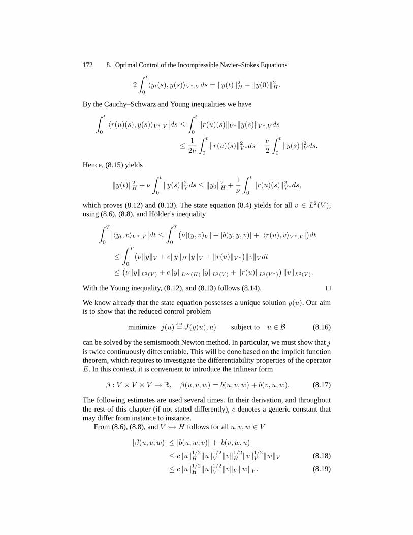
172 8. OptimalControlof theIncompressibleNavier–StokesEquations
2∫ t
0
〈yt(s), y(s)〉V ∗,V ds = ‖y(t)‖2H − ‖y(0)‖2H .
By theCauchy–SchwarzandYounginequalitieswe have∫ t
0
∣∣〈r(u)(s), y(s)〉V ∗,V ∣∣ds ≤ ∫ t
0
‖r(u)(s)‖V ∗‖y(s)‖V ∗,V ds
≤ 12ν
∫ t
0
‖r(u)(s)‖2V ∗ds+ν
2
∫ t
0
‖y(s)‖2V ds.
Hence,(8.15)yields
‖y(t)‖2H + ν
∫ t
0
‖y(s)‖2V ds ≤ ‖y0‖2H +1ν
∫ t
0
‖r(u)(s)‖2V ∗ds,
which proves(8.12)and(8.13).Thestateequation(8.4) yields for all v ∈ L2(V ),using(8.6),(8.8),andHolder’s inequality∫ T
0
∣∣〈yt, v〉V ∗,V ∣∣dt ≤ ∫ T
0
(ν|(y, v)V |+ |b(y, y, v)| + |〈r(u), v〉V ∗,V |
)dt
≤∫ T
0
(ν‖y‖V + c‖y‖H‖y‖V + ‖r(u)‖V ∗
)‖v‖V dt≤ (ν‖y‖L2(V ) + c‖y‖L∞(H)‖y‖L2(V ) + ‖r(u)‖L2(V ∗)
) ‖v‖L2(V ).
With theYounginequality, (8.12),and(8.13)follows (8.14). utWe know alreadythat thestateequationpossessesa uniquesolutiony(u). Our aimis to show thatthereducedcontrolproblem
minimize j(u) def= J(y(u), u) subjectto u ∈ B (8.16)
canbesolvedby thesemismoothNewtonmethod.In particular, wemustshow thatjis twicecontinuouslydifferentiable.Thiswill bedonebasedontheimplicit functiontheorem,whichrequiresto investigatethedifferentiabilitypropertiesof theoperatorE. In this context, it is convenientto introducethetrilinear form
β : V × V × V → R, β(u, v,w) = b(u, v,w) + b(v, u,w). (8.17)
The following estimatesareusedseveral times.In their derivation,andthroughoutthe restof this chapter(if not stateddifferently),c denotesa genericconstantthatmaydiffer from instanceto instance.
From(8.6),(8.8),andV → H follows for all u, v,w ∈ V|β(u, v,w)| ≤ |b(u,w, v)| + |b(v,w, u)|
≤ c‖u‖1/2H ‖u‖1/2V ‖v‖1/2H ‖v‖1/2V ‖w‖V (8.18)
≤ c‖u‖1/2H ‖u‖1/2V ‖v‖V ‖w‖V . (8.19)

8.3 Analysisof theControlProblem 173
Further, (8.18)andHolder’s inequalitywith exponents(∞, 4,∞, 4, 2) yield for allu, v ∈ L2(V ) ∩ L∞(H)← W andall w ∈ L2(V )∫ T
0
|β(u, v,w)|dt ≤ c∫ T
0
‖u‖1/2H ‖u‖1/2V ‖v‖1/2H ‖v‖1/2V ‖w‖V dt
≤ c‖u‖1/2L∞(H)
‖u‖1/2L2(V )
‖v‖1/2L∞(H)
‖v‖1/2L2(V )
‖w‖L2(V ). (8.20)
In particular, for all u, v ∈W andw ∈ L2(V ),∫ T
0
|β(u, v,w)|dt ≤ c‖u‖W‖v‖W ‖w‖L2(V ). (8.21)
Finally, (8.19)andHolder’s inequalitywith exponents(∞, 4, 4, 2) give for all u ∈L2(V ) ∩ L∞(H), v ∈ L4(V ), andw ∈ L2(V )∫ T
0
|β(u, v,w)|dt ≤ c∫ T
0
‖u‖1/2H ‖u‖1/2V ‖v‖V ‖w‖V dt
≤ c‖u‖1/2L∞(H)‖u‖1/2L2(V )‖v‖L4(V )‖w‖L2(V ). (8.22)
Wenow prove thatthestateequationis infinitely Frechetdifferentiable.
Proposition8.5. Lety0 ∈ H and(y, u) ∈W×U . ThentheoperatorE : W×U →Z∗ is twice continuouslydifferentiablewith Lipschitz continuousfirst derivative,constantsecondderivative, andvanishingthird andhigherderivatives.Thederiva-tivesaregivenby:
E′1(y, u)(v,w) = vt + νAv +B(y)v +B(v)y − Rπw, (8.23)
E′2(y, u)(v,w) = v(0, ·), (8.24)
E′′1 (y, u)(v,w)(v, w) = B(v)v +B(v)v, (8.25)
E′′2 (y, u)(v,w)(v, w) = 0. (8.26)
Proof. SinceE2 is linearandcontinuous,theassertionsonE′2 andE′′2 areobvious.Thus,weonly haveto considerE1. If E1 is differentiable,thenformaldifferentiationshows thatE′1 hasthe form statedin (8.23).This operatormaps(v,w) ∈ W × UcontinuouslytoL2(V ∗). In fact,for all z ∈ L2(V ), weobtainusing(8.21)∫ T
0
∣∣〈vt + νAv +B(y)v +B(v)y −Rπw, z〉V ∗,V∣∣dt ≤
≤∫ T
0
(‖vt‖V ∗‖z‖V + ν‖v‖V ‖z‖V + |β(y, v, z)| + ‖Rπw‖V ∗‖z‖V)dt
≤ (‖vt‖L2(V ∗) + ν‖v‖L2(V ) + c‖y‖W‖v‖W + ‖Rπ‖U,L2(V ∗)‖w‖U)‖z‖L2(V ).
Next, weshow thatE1 is differentiablewith its derivativegivenby (8.23).Usingthelinearityof A,B(v), v 7→ B(v), andRπ, weobtainfor all y, v ∈W , u,w ∈ U

174 8. OptimalControlof theIncompressibleNavier–StokesEquations
E1(y + v, u+ w)− E1(y, u)− (vt + νAv + B(y)v +B(v)y −Rπw)= B(y + v)(y + v) −B(y)y − B(y)v −B(v)y = B(v)v.
For all z ∈ L2(V ) holdsby (8.6),(8.8),andHolder’s inequality∫ T
0
∣∣〈B(v)v, z〉V ∗,V∣∣dt =
∫ T
0
|b(v, v, z)|dt ≤∫ T
0
c‖v‖V ‖v‖H‖z‖V dt≤ c‖v‖L2(V )‖v‖L∞(H)‖z‖L2(V ) ≤ c‖v‖2W‖z‖L2(V ),
whichprovestheFrechetdifferentiabilityofE1. NotethatE′1 dependsaffinelinearlyon (y, u) ∈W × U . It remainsto show thatthemapping
E′1 : W × U 7→ L(W × U,L2(V ∗))
is continuousat (0, 0). But this follows from
|〈E′1(y, u)(v,w) −E′1(0, 0)(v,w), z〉V ∗,V | = |β(y, v, z)| ≤ c‖y‖W‖v‖W ‖z‖L2(V ).
for all y, v ∈ W , all u,w ∈ U , andall z ∈ L2(V ), wherewe have used(8.21).As a consequence,E′1 is affine linear and continuous,thus Lipschitz, andE1 istwice continuouslydifferentiablewith constantsecondderivativeasgivenin (8.25).Further, sinceE′′ is constant,it follows thatE(k) = 0 for all k ≥ 3. utThenext resultconcernsthelinearizedstateequationTheproof canbeobtainedbystandardmethods;theinterestedreaderis referredto [79, 80].
Proposition8.6. Let y0 ∈ H and(y, u) ∈ W × U . ThentheoperatorEy(y, u) ∈L(W,Z∗) is a homeomorphism,or, in moredetail: For all y ∈W , g ∈ L2(V ∗), andv0 ∈ H, thelinearizedNavier-Stokesequations
vt + νAv + B(y)v + B(v)y = g in L2(V ∗)v(0, ·) = v0 in H
(8.27)
possessa uniquesolutionv ∈W . Furthermore, thefollowingestimateholds:
‖vt‖L2(V ∗) + ‖v‖L2(V ) + ‖v‖L∞(H) ≤ c‖v‖W (8.28)
≤ c(‖y‖L2(V ), ‖y‖L∞(H))(‖g‖L2(V ∗) + ‖v0‖H) (8.29)
≤ c(‖y‖W )(‖g‖L2(V ∗) + ‖v0‖H), (8.30)
where thefunctionsc(·) dependlocally Lipschitzon their arguments.
Proposition8.7. Themapping
(y, u) ∈ W × U 7→ Ey(y, u)−1 ∈ L(Z∗,W )
is Lipschitz continuouson boundedsets.More precisely, there existsa locally Lips-chitzcontinuousfunctionc such that,for all (yi, ui) ∈ W×U , i = 1, 2, thefollowingholds:
‖Ey(y1, u1)−1 −Ey(y2, u2)−1‖Z∗,W ≤ c(‖y1‖W , ‖y2‖W )‖y1 − y2‖W .

8.3 Analysisof theControlProblem 175
Proof. Let z = (g, v0) ∈ Z∗ = L2(V ∗) × H be arbitraryandset,for i = 1, 2,vi = Ey(yi, ui)−1z. Then,with y12 = y1 − y2, u12 = u1 − u2, andv12 = v1 − v2,wehavev12(0) = 0 and
0 = (E1)y(y1, u1)v1 − (E1)y(y2, u2)v2= (v12)t + νAv12 +B(y1)v1 + B(v1)y1 −B(y2)v2 − B(v2)y2= (v12)t + νAv12 +B(y2)v12 +B(v12)y2 +B(y12)v1 +B(v1)y12= (E1)y(y2, u12)v12 + B(y12)v1 + B(v1)y12,
0 = (E2)y(y1, u1)v1 − (E2)y(y1, u1)v2 = v12(0, ·).
Therefore,
Ey(y2, u12)v12 =(−B(y12)v1 − B(v1)y12
0
),
andthus,by Proposition8.6and(8.21)
‖v12‖W ≤ c(‖y2‖W )(‖B(y12)v1 +B(v1)y12‖L2(V ∗))≤ c(‖y2‖W )‖v1‖W ‖y12‖W≤ c(‖y2‖W )c(‖y1‖W )(‖g‖L2(V ∗) + ‖v0‖H)‖y12‖W≤ c(‖y1‖W , ‖y2‖W )‖y12‖W‖z‖Z∗ ,
wherec(·) arelocally Lipschitzcontinuousfunctions. ut
8.3.2 Control-to-StateMapping
In this sectionwe show that the control-to-statemappingu ∈ U 7→ y(u) ∈ W isinfinitely differentiableandthaty(u), y′(u), andy′′(u) areLipschitzcontinuousonboundedsets.
Theorem8.8. Thesolutionoperator u ∈ U 7→ y(u) ∈ W of (8.10) is infinitelycontinuouslydifferentiable. Further, there exist locally Lipschitz continuousfunc-tionsc(·) such that for all u, u1, u2, v, w ∈ U holds
‖y(u)‖W ≤ c(‖y0‖H , ‖r‖L2(V ∗)), (8.31)
‖y′(u)‖W ≤ c(‖y0‖H , ‖r‖L2(V ∗)), (8.32)
‖y1 − y2‖W ≤ c(‖y0‖H , ‖r1‖L2(V ∗), ‖r2‖L2(V ∗))‖u1 − u2‖U , (8.33)
‖(y′1 − y′2)v‖W ≤ c(‖y0‖H , ‖r1‖L2(V ∗), ‖r2‖L2(V ∗))· ‖Rπ(u1 − u2)‖L2(V ∗)‖Rπv‖L2(V ∗), (8.34)
‖(y′′1 − y′′2 )(v,w)‖W ≤ c(‖y0‖H , ‖r1‖L2(V ∗), ‖r2‖L2(V ∗))· ‖Rπ(u1 − u2)‖L2(V ∗)‖Rπv‖L2(V ∗)‖Rπw‖L2(V ∗), (8.35)
with r = Rπu+ fπ, ri = Rπui + fπ, yi = y(ui), y′i = y′(ui), andy′′i = y′′(ui).

176 8. OptimalControlof theIncompressibleNavier–StokesEquations
Proof. SinceE is infinitely continuouslydifferentiableby Proposition8.5 andthepartialderivativeEy(y(u), u) ∈ L(W,Z∗) is ahomeomorphismaccordingtoPropo-sition8.6,theimplicit functiontheoremyieldsthatu ∈ U 7→ y(u) ∈W is infinitelycontinuouslydifferentiable.
Theestimate(8.31)is justarestatementof (8.14)in Proposition8.4.Using(8.31)andProposition8.6,weseethatthederivativeu ∈ U 7→ y′(u) ∈ L(U,W ) satisfies,settingy = y(u), for all v ∈ U ,
‖y′(u)v‖W = ‖Ey(y, u)−1Eu(y, u)v‖W ≤ ‖Ey(y, u)−1‖Z∗,W ‖Eu(y, u)v‖Z∗≤ c(‖y‖W )‖Eu(y, u)v‖Z∗ ≤ c(‖y0‖H , ‖r‖L2(V ∗))‖Rπv‖L2(V ∗)
with c(·) beinglocally Lipschitz.Thisproves(8.32).Using(8.32),we obtainfor all u1, u2 ∈ U , settingu12 = u1 − u2 andu(τ) =
τu1 + (1− τ)u2,
‖y1 − y2‖W =∫ 1
0
‖y′(u(τ))u12‖W dτ
≤∫ 1
0
c(‖y0‖H , ‖r(u(τ))‖L2(V ∗)
)‖Rπu12‖L2(V ∗)dτ
≤ c(‖y0‖H , ‖r1‖L2(V ∗), ‖r2‖L2(V ∗))‖Rπ(u1 − u2)‖L2(V ∗)
with a locally Lipschitzfunctionc. Therefore,(8.33)is shown.FromProposition8.7,(8.31),and(8.33),weobtain,for all v ∈ U ,
‖(y′1 − y′2)v‖W = ‖Ey(y1, u1)−1Eu(y1, u1)v − Ey(y2, u2)−1Eu(y2, u2)v‖W≤ c(‖y1‖W , ‖y2‖W )‖y1 − y2‖W ‖Rπv‖L2(V ∗)
≤ c(‖y0‖H , ‖r1‖L2(V ∗), ‖r2‖L2(V ∗))‖Rπ(u1 − u2)‖L2(V ∗)‖Rπv‖L2(V ∗)
with c(·) beinglocally Lipschitzcontinuous.This establishes(8.34).Finally, differentiatingtheequationE(y(u), u) = 0 twiceyields,for all u, v,w ∈
U , with y = y(u),
Ey(y, u)y′′(u)(v,w) +Eyy(y, u)(y′(u)v, y′(u)w)+ Eyu(y, u)(y′(u)v,w) + Euy(y, u)(v, y′(u)w) + Euu(y, u)(v,w) = 0.
Now, weusethatEuv = (−Rπv, 0)T is constantto concludethat
y′′(u)(v,w) = −Ey(y, u)−1Eyy(y, u)(y′(u)v, y′(u)w)
= −Ey(y, u)−1(B(y′(u)v)y′(u)w + B(y′(u)w)y′(u)v
).
Fromthis,Proposition8.7,(8.33),and(8.34)weseethat(8.35)holdstrue. ut
8.3.3 Adjoint Equation
Next, givenacontrolu ∈ U andastatey ∈W , weanalyzetheadjointequation

8.3 Analysisof theControlProblem 177
Ey(y, u)∗(wh
)= g, (8.36)
which canbeusedfor therepresentationof thegradientj′(u). In fact,seeappendixA.1, wehavewith y = y(u)
j′(u) = Ju(y, u) + Eu(y, u)∗(w
h
), where Ey(y, u)∗
(w
h
)= −Jy(y, u).
Proposition8.9. 1. For everyu ∈ U andy ∈ W , theadjoint equation(8.36)pos-sessesa uniquesolution(w,h) ∈ Z = L2(V )×H for all g ∈W ∗. Moreover,
‖w‖L2(V ) + ‖h‖H ≤ c‖(w,h)‖Z ≤ c(‖y‖W )‖g‖W ∗, (8.37)
wherec(·) is locally Lipschitz.2. Assumenow that g ∈ L4/3(V ∗) ∩ W ∗. Thenthe adjoint equationcan be
written in theform
− d
dt(w, v)H + ν(w, v)V + β(y, v,w) = 〈g, v〉V ∗,V ∀ v ∈ V on (0, T ), (8.38)
w(T, ·) = 0 onΩ, (8.39)
h− w(0, ·) = 0 onΩ. (8.40)
Furthermore,wt ∈ L4/3(V ∗) ∩W ∗, w ∈ C(V ∗), and
‖wt‖W ∗ ≤ c(‖y‖W )‖g‖W ∗, (8.41)
‖wt‖L4/3(V ∗) ≤ c(‖y‖W )‖g‖W ∗ + ‖g‖L4/3(V ∗) (8.42)
with c(·) beinglocally Lipschitzcontinuous.
Proof. 1. From Proposition8.6 we know thatEy(y, u) ∈ L(W,Z∗) is a homeo-morphismandthusalsoEy(y, u)∗ ∈ L(Z,W ∗) is a homeomorphism.Hence,theadjointequationpossessesauniquesolution(w,h) ∈ Z = L2(V )×H thatdependslinearly andcontinuouslyong ∈W ∗. Moreprecisely, Proposition8.6yields
‖w‖L2(V ∗) + ‖h‖H ≤ c‖(w,h)‖Z = c‖(Ey(y, u)∗)−1g‖Z≤ c‖(Ey(y, u)∗)−1‖W ∗,Z‖g‖W ∗
= c‖Ey(y, u)−1‖Z∗,W ‖g‖W ∗ ≤ c(‖y‖W )‖g‖W ∗,
wherec(·) dependslocally Lipschitzon‖y‖W .2. For the restof the proof we assumeg ∈ W ∗ ∩ L4/3(V ∗). We proceedby
showing that theadjointequationcoincideswith (8.38).Using the trilinear form βdefinedin (8.17),theadjointstate(w,h) ∈ L2(V )×H satisfiesfor all v ∈W :∫ T
0
(〈vt, w〉V ∗,V +ν(v,w)V +β(y, v,w)−〈g, v〉V ∗,V)dt+(v(0), h)H = 0. (8.43)

178 8. OptimalControlof theIncompressibleNavier–StokesEquations
In particular, weobtainfor v ∈W replacedbyϕv with ϕ ∈ C∞0 (0, T ) andv ∈ V :
− d
dt(w, v)H + ν(w, v)V + β(y, v,w) = 〈g, v〉V ∗,V ∀ v ∈ V on (0, T ),
in the senseof distributions,which is (8.38). As a result of (8.22), we have thatz ∈ L4(V ) 7→ β(y, z,w) is linear and continuousand thereforean elementofL4(V )∗ = L4/3(V ∗). For v ∈ V this implies β(y, v,w) ∈ L4/3(0, T ). Further,〈g, v〉V ∗,V ∈ L4/3(0, T ) and(w, v)V ∈ L2(0, T ), hence
d
dt(w, v)H = ν(w, v)V + β(y, v,w) − 〈g, v〉V ∗,V ∈ L4/3(0, T ).
This shows that (w, v)H ∈ H1,4/3(0, T ). For all v ∈ V andall ϕ ∈ C∞([0, T ])holdsϕv ∈ W . We choosetheseparticulartestfunctionsin (8.43)andintegratebyparts(which is allowedsinceC∞([0, T ]) → H1,4(0, T )) Thisgives
0 =∫ T
0
((v,w)Hϕ′ +
(ν(v,w)V + β(y, v,w) − 〈g, v〉V ∗,V
)ϕ)dt+ (v, h)Hϕ(0)
=∫ T
0
(− d
dt(w, v)H + ν(w, v)V + β(y, v,w) − 〈g, v〉V ∗,V
)ϕdt
+ (v, h − w(0))Hϕ(0) + (v,w(T ))Hϕ(T )
Theintegral vanishes,since(8.38)wasalreadyshown to hold.Consideringall ϕ ∈C∞([0, T ]) with ϕ(0) = 0 proves(8.39),whereas(8.40)follows by consideringallϕ ∈ C∞([0, T ]) with ϕ(T ) = 0.
Finally, wesolve(8.38)for wt andapply(8.21)to derive,for all z ∈W ,
〈wt, z〉W ∗,W ≤∫ T
0
(ν|(w, z)V |+ |β(y, z,w)|)dt+ |〈g, z〉W ∗,W |
≤ ν‖w‖L2(V )‖z‖L2(V ) + c‖y‖W‖w‖L2(V )‖z‖W + ‖g‖W ∗‖z‖W .
Further, for all z ∈ L4(V ),∫ T
0
〈wt, z〉V ∗,V dt ≤∫ T
0
∣∣ν(w, z)V + β(y, z,w) − 〈g, z〉V ∗,V∣∣dt
≤ (ν‖w‖L4/3(V ) + c‖y‖W‖w‖L2(V ) + ‖g‖L4/3(V ∗))‖z‖L4(V ),
wherewehaveusedHolder’s inequalityand(8.22).Applicationof (8.37)completestheproof of (8.41)and(8.42).Theassertionw ∈ C(V ∗) follows from theembed-dingw ∈ L2(V ) : wt ∈ L4/3(V ∗) → C(V ∗). utOur next aim is to estimatethedistanceof two adjointstates(wi, hi), i = 1, 2, thatcorrespondto differentstatesyi andright handsidesgi.

8.3 Analysisof theControlProblem 179
Proposition8.10. For given yi ∈ W and gi ∈ W ∗ ∩ L4/3(V ∗), i = 1, 2, let(wi, hi) ∈ L2(V ) × H denotethe correspondingsolutionsof the adjoint equa-tion (8.36) with state yi and right hand side gi. Thenwi ∈ L2(V ) ∩ C(V ∗),(wi)t ∈ W ∗ ∩ L4/3(V ∗), hi = wi(0), and
‖w1 − w2‖L2(V ) + ‖(w1 − w2)t‖L4/3(V ∗) + ‖h1 − h2‖H≤ c(‖y1‖W , ‖y2‖W )
(‖g1 − g2‖W ∗ + ‖g1‖W ∗‖y1 − y2‖W)
+ ‖g1 − g2‖L4/3(V ∗),
(8.44)
wherec(·) is locally Lipschitzcontinuous.
Proof. The existenceandregularity resultsarethosestatedin Proposition8.9. In-troducingthe differencesw12 = w1 − w2, h12 = h1 − h2, y12 = y1 − y2, andg12 = g1 − g2, wehavew12(T ) = 0 andh12 = w12(0) onΩ and,on (0, T ),
− d
dt(w12, v)H + ν(w12, v)V + β(y1, v, w1)− β(y2, v, w2) = 〈g12, v〉V ∗,V .
Rearrangingtermsyields
− d
dt(w12, v)H + ν(w12, v)V + β(y2, v, w12) = 〈g12, v〉V ∗,V − β(y12, v, w1).
Therefore,(w12, h12) is solutionof theadjointequationfor thestatey2 andtherighthandside
g = g12 − `, ` : v 7→ β(y12, v, w1).
From(8.21),(8.22)weknow that` ∈W ∗ ∩ L4/3(V ∗) and
‖`‖W ∗ + ‖`‖L4/3(V ∗) ≤ c‖y12‖W ‖w1‖L2(V ).
Therefore,by Proposition8.9
‖w12‖L2(V ) + ‖(w12)t‖L4/3(V ∗) + ‖h12‖H ≤ c(‖y2‖W )‖g‖W ∗ + ‖g‖L4/3(V ∗)
≤ c(‖y2‖W )(‖g12‖W ∗ + c‖w1‖L2(V )‖y12‖W
)+ ‖g12‖L4/3(V ∗)
+ c‖w1‖L2(V )‖y12‖W≤ c(‖y2‖W )
(‖g12‖W ∗ + ‖w1‖L2(V )‖y12‖W)
+ ‖g12‖L4/3(V ∗)
≤ c(‖y2‖W )(‖g12‖W ∗ + c(‖y1‖W )‖g1‖W ∗‖y12‖W
)+ ‖g12‖L4/3(V ∗)
≤ c(‖y1‖W , ‖y2‖W )(‖g12‖W ∗ + ‖g1‖W ∗‖y12‖W
)+ ‖g12‖L4/3(V ∗),
wherec(·) is locally Lipschitz.Theproof is complete. ut
8.3.4 Propertiesof the ReducedObjectiveFunction
We will now show that thereducedobjective functionj meetsall requirementsthatare neededto apply semismoothNewton methodsfor the solution of the controlproblem(8.16).Wehave,sinceJ is quadratic,

180 8. OptimalControlof theIncompressibleNavier–StokesEquations
Ju(y, u) = λ(u− ud), Jy(y, u) = Nπ∗(Nπy − zd),Juu(y, u) = λI, Juy(y, u) = 0,Jyu(y, u) = 0, Jyy(y, u) = Nπ∗Nπ.
Since,u ∈ U 7→ y(u) ∈ W is infinitely differentiableandy, y′, andy′′ areLipschitzcontinuouson boundedsets,seeTheorem8.8,we obtainthatj(u) = J(y(u), u) isinfinitely differentiablewith j, j′, and j′′ beingLipschitz continuouson boundedsets.
Further, usingtheadjointrepresentationof thegradient,andthefactthatEuv =(−Rπv, 0)T , wehave,with y = y(u),
j′(u) = Ju(y, u)−Rπ∗w = λ(u− ud)−R∗w, (8.45)
wherew solvestheadjointequation(8.38),(8.39)with right handside
g = −Jy(y, u) = −Nπ∗(Nπy − zd) ∈ L2(V ∗) →W ∗ ∩ L4/3(V ∗). (8.46)
Therefore,wehave:
Theorem8.11. Thereducedobjectivefunctionj : U = L2(Qc)l → R is infinitelydifferentiablewith j, j′, and j′′ beingLipschitz continuouson boundedsets.Thereducedgradienthastheform
j′(u) = λu+G(u),G(u) = −R∗w − λud,
wherew is theadjoint state. In particular, theoperatorG mapsL2(Qc)l Lipschitzcontinuouslyon boundedsetsto Lp
′(Qc)l. Further, G : L2(Qc)l → L2(Qc)l is
continuouslydifferentiablewithG′(u) = G′(u)∗ beingboundedon boundedsetsinL(L2(Qc)l, Lp
′(Qc)l)
Proof. Thepropertiesof j follow from Theorem8.8and(8.45).TheLipschitzcon-tinuity assertionon G follows from (8.44), (8.33), and (8.46). Further, G(u) =j′(u) − λu is, consideredas a mappingL2(Qc)l → L2(Qc)l, continuouslydif-ferentiablewith derivative G′(u) = j′′(u) − λI. In particular, we seethatG′ isself-adjoint.Now considerG′(u) for all u ∈ Bρ = ρBL2(Qc)l . On this setG maps
Lipschitz continuouslyinto Lp′(Qc)l. Denotingthe Lipschitz rank by Lρ, we now
prove ‖G′(u)‖L2(Qc)l,Lp′ (Qc)l ≤ Lρ for all u ∈ Bρ. In fact, for all u ∈ Bρ andall
v ∈ L2(Qc)l wehaveu+ tv ∈ Bρ for t > 0 smallenoughandthus
‖G′(u)v‖Lp′ (Qc)l = limt→0+
t−1‖G(u+ tv)−G(u)‖Lp′(Qc)l ≤ Lρ‖v‖L2(Qc)l .
utFor illustration,weconsiderthecasewhereΩc ⊂ Ω, l = 2, and
(Rv)(x) = v(x) for x ∈ Ωc, (Rv)(x) = 0, otherwise.
Weneedthefollowing embedding:

8.4 Applicationof SemismoothNewton Methods 181
Lemma 8.12. For all 1 ≤ p < 7/2 andall v ∈ L2(V ) with vt ∈ L4/3(V ∗) holds
‖v‖Lp(Q)2 ≤ c(‖vt‖L4/3(V ∗) + ‖v‖L2(V )
).
Proof. In [7] it is provedthatfor all 1 ≤ q < 8 holds
W 4/3 = v ∈ L2(V ) : vt ∈ L4/3(V ∗) → Lq(H)
(theembeddingis evencompact).We proceedby showing that for all p ∈ [1, 7/2)thereexistsq ∈ [1, 8) suchthatLq(H)∩L2(V ) → Lp(Q)2. Dueto theboundednessof Q it sufficesto considerall p ∈ [2, 7/2). Recall thatV → Ls(Ω)2 for all s ∈[1,∞). Now let r = 4, r′ = 4/3,
θ = 1− 32p∈ [1/4, 4/7) and s =
67− 2p
∈ [2,∞).
Thenholds
θ
2+
1− θs
=1p,
1r
+1r′
= 1,
q = θpr = 4p− 6 ∈ [2, 8), (1− θ)pr′ = 2.
Thus,we canapplytheinterpolationinequalityandHolder’s inequalityto conclude
‖v‖pLp(Q)2 =∫ T
0
‖v‖pLp(Ω)2dt ≤ c∫ T
0
‖v‖θpL2(Ω)2‖v‖(1−θ)pLs(Ω)2dt
≤ c(∫ T
0
‖v‖θprL2(Ω)2dt
)1/r (∫ T
0
c‖v‖(1−θ)pr′Ls(Ω)2 dt
)1/r′
= c‖v‖θpLq(H)2‖v‖(1−θ)pL2(Ls(Ω)2)
≤ c(‖vt‖L4/3(V ∗) + ‖vt‖L2(V )
)θp‖v‖(1−θ)pL2(V )
≤ c(‖vt‖L4/3(V ∗) + ‖vt‖L2(V )
)p.
utFor 2 < p′ < 7/2 wethushave that
w ∈W 4/3 → Lp′(Q)2 7→ R∗w = w|Qc
∈ Lp′(Qc)2
is continuous,sothatTheorem8.11is applicable.
8.4 Application of SemismoothNewtonMethods
Wenow considerthereducedproblem(8.16)with feasiblesetof theform (8.3),andreformulateits first ordernecessaryoptimality conditionsin form of thenonsmoothoperatorequation

182 8. OptimalControlof theIncompressibleNavier–StokesEquations
Π(u) = 0,
Π(u)(t, ω) = u(t, ω)− PC(u(t, ω)− λ−1j′(u)(t, ω)
), (t, ω) ∈ Qc.
Let usassumethatPC is semismooth.Then,for r = 2 andany p′ asspecified,The-orem8.11shows thatAssumption5.14is satisfiedby F = j′. Therefore,Theorem5.15is applicableandyieldsthe∂CΠ-semismoothnessofΠ : L2(Qc)l → L2(Qc)l.
If wepreferto work with a reformulationby meansof adifferentLipschitzcon-tinuousandsemismoothfunctionπ,
π(x) = 0 ⇐⇒ x1 − PC(x1 − x2) = 0,
in theformπ(u, j′(u)
)= 0,
wecanuseTheorem5.11toestablishthesemismoothnessof theresultingoperatorasa mappingLp(Qc)l → L2(Qc)l for any p ≥ p′. Therefore,ourclassof semismoothNewtonmethodsis applicableto bothreformulations.
We alsocanapply thesufficient conditionfor regularity of Theorem4.8.Sincethis conditionwasestablishedin theframework of NCPs,we considernow thecaseU = L2(Qc) andC = [0,∞). Then,we immediatelyseethat Theorem8.11pro-videseverythingto verify Assumption4.6, provided that j′′(u) is coercive on thetangentspaceof thestronglyactive constraintsasassumedin (e) andthat theusedNCP-functionπ = φ satisfies(f)–(h). Thecoercivity conditioncanbeinterpretedasastrongsecondordersufficientconditionfor optimality, see[46, 143].
We arecurrentlyworking on a finite-elementdiscretizationof the flow controlproblemandhopeto have numericalresultsavailablesoon.In the implementationof themethodwe planto usea preconditionediterative method(gmres,cg,etc.)forthe solutionof the semismoothNewton system.Hereby, dependingon the particu-lar problem,reductiontechniquescanbeusedto symmetrizethesemismoothNew-ton system,which makesconjugategradientmethodsapplicable.Theencouragingnumericalresultsby Hinze andKunisch[80] for second-ordermethodsappliedtotheunconstrainedcontrolof theNavier-Stokesequationmake usconfidentthat thesemismoothNewtonmethodcanbesolvedefficiently.

9. Optimal Control of the CompressibleNavier–StokesEquations
9.1 Intr oduction
In this chapterwe apply our classof semismoothNewton methodsto a boundarycontrolproblemgovernedby thetime-dependentcompressibleNavier–Stokesequa-tions.The underlyingNavier–Stokessolver andthe adjoint codefor the computa-tion of the reducedgradientweredevelopedin joint work with ScottCollis (RiceUniversity),MatthiasHeinkenschloss(RiceUniversity),KavehGhayour(RiceUni-versity), andStefan Ulbrich (TU Munchen)aspart of the the Rice AeroAcousticControl (RAAC) project,which was initiated and is directedby Scott Collis andMatthiasHeinkenschloss.Themajoraimof this projectis to put forwardanoptimalcontrol framework for the control of aeroacousticnoisewherethe acousticsourceis predictedby theunsteady, compressible,Navier-Stokesequations.A particularlyinterestingapplicationis the control of the soundarisingfrom Blade-Vortex Inter-action (BVI), which can occur for rotorcraft undercertainflight conditions(e.g.,during landing).Hereby, vorticesshedby a precedingbladehit a subsequentbladewhich resultsin ahighamplitude,impulsivenoise.This loudnoiserestrictscivil ro-torcraftuseseverely, andthusmakesactivenoisecontrolonthebladesurfacehighlydesirable.For moredetailswe referto [34, 35] andthereferencestherein.
9.2 The Flow Control Problem
In the following, we will not considernoisecontrol.Rather, we contentourselveswith solvingamodelproblemto investigatetheviability of ourapproachfor control-ling thecompressibleNavier–Stokesequations.Thismodelconsistsin two counter-rotatingviscousvorticesaboveaninfinite wall which,dueto theself-inducedveloc-ity field, propagatedownwardandinteractwith thewall. As controlmechanismweusesuctionandblowing on partof thewall, i.e., we control thenormalvelocity ofthefluid on this partof thewall. As computationaldomainwe usea rectangle
Ω = (−L1, L1)× (0, L2).
Thewall is locatedatx2 ≡ 0, whereastheleft, right, andupperpartof theboundaryare“transparent”in thesensethatwe posenonreflectingboundaryconditionsthere.Ω is occupiedby a compressiblefluid whosestateis describedby y = (ρ, v1, v2, θ)

184 9. OptimalControlof theCompressibleNavier–StokesEquations
with densityρ(t, x), velocitiesvi(t, x), i = 1, 2, andtemperatureθ(t, x). Hereby,t ∈ I def= (0, T ) is the time andx = (x1, x2) denotesthespatiallocation.Thestatesatisfiesthe
CompressibleNavier–StokesEquations (CNS):
∂
∂tF 0(y) +
2∑i=1
∂
∂xiF i(y) =
2∑i=1
∂
∂xiGi(y,∇y) on I ×Ω,
y(0, ·) = y0 on Ω.
Hereby, we have written CNSin conservative form. Boundaryconditionsarespeci-fied below. Wehaveusedthefollowing notation:
F 0(y) =
ρρv1ρv2ρE
, F 1(y) =
ρv1
ρv21 + pρv1v2
(ρE + p)v1
, F 2(y) =
ρv2ρv1v2ρv2
2 + p(ρE + p)v2
,
Gi(y,∇y) =1
Re
0τ1iτ2i
τ1iv1 + τ2iv2 +κ
(γ − 1)M2Prθxi
.
Thepressurep, thetotalenergy perunit massE, andthestresstensorτ aregivenby
p =ρθ
γM2, E =
θ
γ(γ − 1)M2+
12(v2
1 + v22),
τii = 2µ(vi)xi+ λ(∇ · v), τ12 = τ21 = µ((v1)x2 + (v2)x1).
Hereµ andλ arethefirst andsecondcoefficient of viscosity, κ is the thermalcon-ductivity, M is thereferenceMachnumber, Pr is thereferencePrandtlnumber, andReis thereferenceReynoldsnumber. Theboundaryconditionson thewall are
∂θ/∂n = 0, v1 = 0, v2 = u on Σc = I × (−L1, L1)× 0,andon therestof theboundarywe posenonreflectingboundaryconditionsthatarederivedfrom inviscidcharacteristicboundaryconditions.
At the initial time t = 0 two counter-rotating viscousvorticesare locatedinthe centerof Ω. Without control (v2 = u ≡ 0), the vorticesmove downward andinteractwith thewall, whichcausesthemto bounceback,seeFigure9.1.Ouraim isto performcontrolby suctionandblowing onthewall in suchawaythattheterminalkinetic energy is minimized.To this end,wechoosetheobjective function
J(y, u) =∫Ω
[ρ2(v2
1 + v22)]t=T
dx+α
2‖u‖2H1(Σc)
.
The first term is the kinetic energy at the final time t = T , whereasthe secondterm is anH1-regularizationwith respectto (t, x1). Here,we write α > 0 for the

9.3 Adjoint-BasedGradientComputation 185
regularizationparameterto avoid confusionwith thesecondcoefficientof viscosity.As controlspace,we chooseU = H1(I,H1
0 (−L1, L1)). We stressthat themathe-maticalexistenceanduniquenesstheoryfor thecompressibleNavier–Stokesequa-tions,see[81, 108, 111] for stateof theart references,seemsnot yet to becompleteenoughto admitarigorouscontroltheory. Therefore,ourchoiceof thecontrolspaceis guidedmoreby formal andheuristicargumentsthanby rigorouscontrol theory.If theH1-regularizationis omittedor replacedby anL2-regularization,thecontrolexhibits increasinglyheavy oscillationsin time andspaceduringthecourseof opti-mization,which indicatesthat theproblemis ill-posedwithout a sufficiently strongregularization.
In theRAAC project,we consideredso far only theunconstrainedflow controlproblemandworkedwith a nonlinearconjugategradientmethodfor its solution.Inthe following, we want to solve the sameproblem,but with the control subjecttopointwiseboundconstraints.We thenapplyour inexactsemismoothNewton meth-odsanduseBFGS-updates[41, 42] to approximatetheHessianof thereducedob-jective function. Therefore,in the following we restrict the control by pointwiseboundconstraints(with therealisticinterpretationthatwe areonly allowedto injector draw off fluid with a certainmaximumspeed),andarrive at the following flowcontrolproblem:
minimize J(y, u) def=∫Ω
[ρ2(v2
1 + v22)]t=T
dx+α
2‖u‖2H1(Σc)
subjectto y solvesCNSfor theboundaryconditionsassociatedwith u,
umin ≤ u ≤ umax.
(9.1)
9.3 Adjoint-Based Gradient Computation
For our computationswe usethe following resultsthat wereobtainedjointly withScottCollis,KavehGhayour, MatthiasHeinkenschloss,andStefanUlbrich [34, 35]:
1. A Navier–Stokessolver, written in Fortran90by ScottCollis [36], wasportedtotheparallelcomputerSGI Origin 2000andadjustedto therequirementsof optimalcontrol. For spacediscretizationfinite differencesare usedwhich are sixth orderaccuratein theinterior of thedomain.Thetime discretizationis doneby anexplicitRunge–Kuttamethod.Thecodewasparallelizedon thebasisof OpenMP.
2. Two differentvariantsof adjoint-basedgradientcomputationwereconsidered:
(a) The first approachderives the adjoint Navier–Stokesequationsincluding ad-joint wall boundaryconditions[35]. Thederivationof adjointboundarycondi-tionsfor thenonreflectingboundaryconditionsturnsout to beadelicatematterandis not yet completelydone.Hence,in this approachwe have usedthe(ap-propriatelyaugmented)adjointboundaryconditionsof theEulerequation.Thegradientcalculationthenrequiresthesolutionof theNavier–Stokesequations,followed by the solutionof the adjoint Navier–Stokesequationsbackward in

186 9. OptimalControlof theCompressibleNavier–StokesEquations
time. Sincethe discretizedadjoint equationis usuallynot the exact adjoint ofthediscretestateequation,this approach,whichusuallyis calledoptimize, thendiscretize(OD), only yieldsinexactdiscretegradientsin general.
(b) In asecondapproachwehaveinvestigatedtheadjoint-basedcomputationof gra-dientsby applyingthereversemodeof automaticdifferentiation(AD). Hereby,weusedtheAD-softwareTAMC [59], asource-to-sourcecompiler, whichtrans-latesFortran90routinesto their correspondingadjointFortran90routines.Thisapproachyields exact (up to roundoff errors)discretegradientsandis termeddiscretize, thenoptimize(DO).
For the computationalresultsshown below, the DO methoddescribedin (b) wasused.This approachhastheadvantageof providing exactdiscretegradients,whichis very favorablewhendoing optimization.In fact, descentmethodsbasedon in-exactgradientsrequirea controlmechanismover theamountof inexactness,whichis not a trivial task in OD basedapproaches.Secondly, the useof exact gradientsis very helpful in verifying the correctnessof the adjoint code,sincepotentialer-rorscanusuallybefoundimmediatelyby comparingdirectionalderivativeswith thecorrespondingfinite differencequotients.
Whenworking with theOD approach,which hastheadvantagethat thesourcecodeof theCNS-solver is not required,thediscretizationof stateequation,adjointequation,andobjectivefunctionhaveto becompatible(in asensenotdiscussedhere,see,e.g.,[34,74]) to obtaingradientsthataregoodapproximations(i) of theinfinite-dimensionalgradients,and(ii) of theexactdiscretegradients.Hereby, requirement(ii) is importantfor asuccessfulsolutionof thediscretecontrolproblem,whereas(i)crucially influencesthequality of thecomputeddiscreteoptimalcontrol,measuredin termsof the infinite-dimensionalcontrolproblem.This secondissuealsoappliesto theDO approach,but for DO it is only importantto usecompatiblediscretizationsfor stateequationandobjective function.With respectto this interestingtopic, wehaveused[74] asa guideline,to whichwereferfor furtherreference.
9.4 SemismoothBFGS-NewtonMethod
Theimplementationof thesemismoothNewtonmethodusesBFGS-approximationsof the Hessianmatrix. The resultingsemismoothNewton systemshave a similarstructureasthosearisingin thestepcomputationof thesuccessfulLimited-MemoryBFGSmethodL-BFGS-B by Byrd, Lu, NocedalandZhu [25, 148]. Hence,in ourimplementationwedecidedto follow thedesignof L-BFGS-B(thecomputationsforthis chapterweredonebeforewedevelopedour trust–region theoryin section6).
9.4.1 Quasi-NewtonBFGS-Approximations
In thissection,wefocusontheuseof BFGS-approximationsin semismoothNewtonmethodsfor the discretizedcontrol problem.We stress,however, that convergence

9.4 SemismoothBFGS-Newton Method 187
resultsfor quasi-Newton methodsin infinite-dimensionalHilbert spacesareavail-able[64, 94, 131]. Usingasimilar notationasin chapter7, thesemismoothNewtonsystemfor thediscretecontrolproblemassumestheform (written in coordinatesinthediscreteL2-space)
[Dh1 ]k + [Dh
2 ]kHhkshk = −Φh(uhk)
with Hhk = jh
′′(uhk) anddiagonalmatrices[Dhi ]k, |([Dh
1 ]k + [Dh2 ]k)jj | ≥ κ.
For theapproximationof theHessianHhk wework with
Limited-Memory BFGS-Matrices (l ≈ 10):
Bhk = Bh
0 −WhkZ
hkW
hk
T ∈ Rnh×nh
, Whk ∈ Rn
h×2l, Zhk ∈ R2l×2l,
wherewehaveusedthecompactrepresentationof [26], to whichwereferfor details.The matrix Bh
0 is the initial BFGS-matrixandshouldbe chosensuchthat (a) theproduct(Bh
0)−1vh canbecomputedreasonablyefficient,sincethis is neededin theBFGS-updates,and(b) the innerproductinducedby Bh
0 approximatestheoriginalinfinite-dimensionalinner producton U sufficiently well. In the caseof our flowcontrol problem,we have U = H1(I,H1
0 (−L1, L1)), andusea finite differenceapproximationof the underlyingLaplaceoperatorto obtain Bh
0 . Comparedwiththestateandadjointsolves,thesolutionof the2-D Helmholtzequationrequiredtocompute(Bh
0)−1vh is negligible. The inverseof Mhk = [Dh
1 ]k + [Dh2 ]kBh
k canbecomputedby theSherman–Morrison–Woodbury formula:
(Mhk)−1 = Ch
k + Chk [D
h2 ]kWh
k
(I − ZhkW
hk
TChk [D
h2 ]kWh
k
)−1ZhkW
hk
TChk ,
whereChk = ([Dh
1 ]k + [Dh2 ]kBh
0)−1.
9.4.2 The Algorithm
Wenow giveasketchof thealgorithm:
1. TheHessianmatrix of thediscreteobjective function is approximatedby Lim-ited-MemoryBFGS-matrices.Hereby, we chooseBh
0 suchthat it representsafinite differenceapproximationof theinnerproductonU .
2. Theglobalizationis similarasin thewell-acceptedL-BFGS-Bmethodof Byrd,Lu, NocedalandZhu [25, 148]:
i. At thecurrentpointuhk ∈ Bh, theobjectivefunctionjh is approximatedbyaquadraticmodelqhk .
ii. Startingfrom uhk , a generalizedCauchypoint uh,ck ∈ Bh is computedbyanArmijo-type linesearchfor qhk alongtheprojectedgradientpath
PBh(uhk − tjhk′), t ≥ 0.
iii. ThesemismoothNewtonmethodis usedto computeaNewtonpointuh,nk .
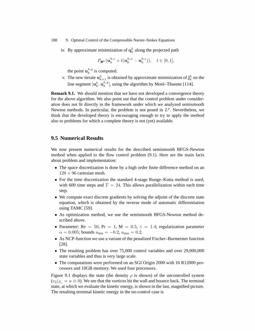
188 9. OptimalControlof theCompressibleNavier–StokesEquations
iv. By approximateminimizationof qhk alongtheprojectedpath
PBh(uh,ck + t(uh,nk − uh,ck )), t ∈ [0, 1],
thepointuh,qk is computed.
v. Thenew iterateuhk+1 is obtainedby approximateminimizationof jhk onthe
line segment[uhk ,uh,qk ], usingthealgorithmby More–Thuente[114].
Remark 9.1. We shouldmentionthatwe have not developeda convergencetheoryfor theabovealgorithm.We alsopoint out that thecontrolproblemunderconsider-ation doesnot fit directly in the framework underwhich we analyzedsemismoothNewton methods.In particular, the problemis not posedin Lp. Nevertheless,wethink that the developedtheory is encouragingenoughto try to apply the methodalsoto problemsfor whichacompletetheoryis not (yet) available.
9.5 Numerical Results
We now presentnumerical resultsfor the describedsemismoothBFGS-Newtonmethodwhen appliedto the flow control problem(9.1). Here are the main factsaboutproblemandimplementation:
• Thespacediscretizationis doneby a high orderfinite differencemethodon an128× 96 cartesianmesh.
• For the time discretizationthe standard4-stageRunge–Kutta methodis used,with 600 time stepsandT = 24. This allows parallelizationwithin eachtimestep.
• We computeexactdiscretegradientsby solvingtheadjointof thediscretestateequation,which is obtainedby the reversemodeof automaticdifferentiationusingTAMC [59].
• As optimizationmethod,we usethe semismoothBFGS-Newton methodde-scribedabove.
• Parameter:Re = 50, Pr = 1, M = 0.5, γ = 1.4; regularizationparameterα = 0.005; boundsumin = −0.2, umax = 0.2.
• As NCP-functionweuseavariantof thepenalizedFischer–Burmeisterfunction[28].
• The resultingproblemhasover 75,000control variablesandover 29,000,000statevariablesandthusis very largescale.
• ThecomputationswereperformedonanSGIOrigin 2000with 16R12000pro-cessorsand10GBmemory. Weusedfour processors.
Figure 9.1 displaysthe state(the densityρ is shown) of the uncontrolledsystem(v2|Σc
= u ≡ 0). Weseethatthevorticeshit thewall andbounceback.Theterminalstate,atwhichweevaluatethekineticenergy, is shown in thelast,magnifiedpicture.Theresultingterminalkineticenergy in theno-controlcaseis

9.5 NumericalResults 189
No control(v2|Σc= u ≡ 0): Ekin|t=T = J(y(0), 0) = 7.9.
Figure9.2 shows the state(representedby the densityρ) whenoptimal control isapplied.Hereby, the optimal control wasobtainedby 100 iterationsof the BFGS-Newton method.The resultingterminalkinetic energy in the optimal control caseandtheobjective functionvalue(Ekin|t=T + regularization), respectively, are
Optimalcontrol(v2|Σc= u∗): Ekin|t=T = 0.059, J(u∗, y(u∗)) = 0.085,
whereu∗ denotesthe computedoptimal control,which is displayedin Figure9.3.It canbeseenin Figure9.3 that the lower boundbecomesactive. In fact, theupperboundalso is active at a few points,but this is not apparentfrom the picture.By
−15−10
−50
510
150
4
8
12
16
20
24
−0.2
0
0.2
x1
t
Figure9.3Computedoptimalcontrolu∗.
applyingoptimalcontrolthevorticesaresuccessfullyabsorbed.If wehaddisplayedthe kinetic energy insteadof the density, the vorticeswould be almostinvisible atthe terminaltime in theoptimalcontrol case,sincetheoptimalcontrol reducestheterminalkinetic energy to lessthanonehundredthof its valuewithout control. Incomparisonwith our computationalexperiencefor theunconstrainedcontrolprob-lem, the semismoothNewton methodperformscomparablyefficient. This showsthe efficiency of semismoothNewton methodsfor the solutionof very large scaleproblems.

A. Appendix
A.1 Adjoint Approachfor Optimal Control Problems
In this appendixwe describethe adjoint approachfor the computationof gradientandHessianof thereducedobjective function.Hereby, we considertheabstractop-timal controlproblem
minimizey∈Y,u∈U
J(y, u) subjectto E(y, u) = 0, u ∈ Uad (A.1)
with feasiblesetUad ⊂ U , objective function
J : Y × U → R,
andstateequationoperatorE : Y × U →W ∗.
Thecontrol spaceU andthestatespaceY areBanachspaces,andW ∗ is the dualof a reflexive BanachspaceW . We assumethe existenceof a neighborhoodV ofUad suchthat, for all u ∈ V , the stateequationE(y, u) = 0 possessesa uniquesolution y = y(u). Then the control problem(A.1) is equivalent to the reducedcontrolproblem
minimize j(u) subjectto u ∈ Uad, (A.2)
wherej : U ⊃ V → R, j(u) = J(y(u), u) is thereducedobjective function.
A.1.1 Adjoint Representationof the ReducedGradient
We now describethe adjoint approachfor the computationof j′(u). To this end,we assumethat J andE are Frechetdifferentiablenear(y(u), u) and that u 7→y(u) is Frechetdifferentiablenearu. Accordingto theimplicit functiontheorem,thelatterholds,e.g.,if E is continuouslydifferentiablenear(y(u), u) andif thepartialderivative Ey(y(u), u) is continuouslyinvertible. Under the given hypothesesthefunctionj is differentiablenearu.
We introducea Lagrangemultiplier w ∈ W for thestateequationin (A.1) anddefinetheLagrangefunctionL : Y × V ×W → R,
L(y, u,w) = J(y, u) + 〈E(y, u), w〉W ∗,W .

192 A. Appendix
SinceE(y(u), u) = 0 onV , we have
L(y(u), u,w) = J(y(u), u) = j(u) ∀ u ∈ V, w ∈ W.
Hence,
j′(u) = yu(u)∗Ly(y(u), u,w) + Lu(y(u), u,w) ∀ u ∈ V, w ∈W. (A.3)
Theideanow is to choosew ∈W suchthat
Ly(y(u), u,w) = 0.
This equationis calledadjoint equationand its solutionw = w(u) ∈ W is theadjoint state. Thus,written in detail, the adjoint statew = w(u) is the solutionoftheadjointequation
Jy(y(u), u) +Ey(y(u), u)∗w = 0.
If we assumethat Ey(y(u), u) is continuouslyinvertible, the adjoint statew isuniquelydetermined.Forw = w(u) weobtain
j′(u) = yu(u)∗Ly(y(u), u,w(u)) + Lu(y(u), u,w(u))= Lu(y(u), u,w(u)) = Ju(y(u), u) +Eu(y(u), u)∗w(u).
Theidentityj′(u) = Ju(y(u), u) + Eu(y(u), u)∗w(u)
is calledadjoint representationof thereducedgradientj′(u).Therefore,thederivativej′(u) canbecomputedasfollows:
1. Computethestatey = y(u) ∈ Y by solvingthestateequation
E(y, u) = 0.
2. Computetheadjointstatew = w(u) ∈ W by solvingtheadjointequation
Ey(y, u)∗w = −Jy(y, u).
3. Computej′(u) = Ju(y, u) + Eu(y, u)∗w.
Remark A.1. If thestateequationis aninitial valueproblem,thentheadjointequa-tion is reversein time. For the derivation of adjoint equationsfor varioustypesofcontrolproblemsgovernedby PDEs,wereferto Lions [106].
A.1.2 Adjoint Representationof the ReducedHessian
The adjoint approachcanbe continuedto obtainadjoint formulasfor the Hessianoperatorj′′(u). To this end,we assumethatJ andE aretwice differentiablenear
A.1 Adjoint Approachfor OptimalControlProblems 193
(y(u), u) andthatu 7→ y(u) is twice differentiablenearu. By (A.3), we have, forall w ∈ W andall v1, v2 ∈ U , writing y = y(u),
j′′(u)(v1, v2) = Lyu(y, u,w)(yu(u)v1, v2) + Lyy(y, u,w)(yu(u)v1, yu(u)v2)+ 〈Ly(y, u,w), yuu(u)(v1, v2)〉Y ∗,Y + Luy(y, u,w)(v1, yu(u)v2)+ Luu(y, u,w)(v1, v2).
If wechoosew = w(u), thenLy(y(u), u,w) = 0, andthus
j′′(u) = T (u)∗L′′(y,u)(y(u), u,w(u))T (u), (A.4)
whereL′′(y,u) denotesthesecondpartialderivativewith respectto (y, u), and
T (u) =(yu(u)IU
)=(−Ey(y(u), u)−1Eu(y(u), u)
IU
).
Hereby, in thesecondexpressionfor T (u) we assumethatEy(y(u), u) is continu-ouslyinvertibleandusethat,sinceE(y(·), ·) ≡ 0, thereholds
Ey(y(u), u)yu(u) +Eu(y(u), u) = 0.
Remark A.2. It is interestingto notethatin thecasewhereEy(y(u), u) is continu-ously invertible,themappingT (u) is a continuouslinearhomeomorphismfrom Uto the null spaceof E′(y(u), u). In fact, it is obvious thatE′(y(u), u)T (u) = 0.Conversely, if Ey(y(u), u)h+Eu(y(u), u)v = 0, then
h = −Ey(y(u), u)−1Eu(y(u), u)v,
andthus (h
v
)= T (u)v.
Therefore,j′′(u) is the restrictionof the HessianL′′(y,u)(y(u), u,w(u)) of the La-grangianto thenull spaceof E′(y(u), u), parameterizedby v ∈ U 7→ T (u)v.
Usually, the formula (A.4) is not usedto computethe completeHessianoperator.Rather, it is usedto computedirectionalderivativesj′′(u)v of j′. Hereis therequiredprocedure:
1. Computethestatey = y(u) ∈ Y by solvingthestateequation
E(y, u) = 0.
2. Computetheadjointstatew = w(u) ∈ W by solvingtheadjointequation
Ey(y, u)∗w = −Jy(y, u).3. Computez = z(u) ∈ Y assolutionof thelinearizedstateequation
Ey(y, u)z = −Eu(y, u)v.4. Computeh = h(u) ∈W by solvingtheadjointsystem
Ey(y, u)∗h = −Lyy(y, u,w)z − Lyu(y, u,w)v.
5. Setj′′(u)v := Eu(y, u)∗h+ Luy(y, u,w)z + Luu(y, u,w)v.

194 A. Appendix
A.2 Several Inequalities
For convenience,we recall several well-known inequalities,which are frequentlyusedthroughoutthis work.
Lemma A.3 (Holder’s inequality). Let pi ∈ [1,∞], i = 1 . . . , n, andp ∈ [1,∞]satisfy
1p1
+ · · · + 1pn
=1p.
Then,for all fi ∈ Lpi(Ω) holdsf = f1f2 · · · fn ∈ Lp(Ω) and
‖f‖Lp ≤ ‖f1‖Lp1 · · · ‖fn‖Lpn .
Thefollowing estimateis frequentlyusedin chapter3. It follows immediatelyfromHolder’s inequality.
Lemma A.4. LetΩ bebounded,1 ≤ p ≤ q ≤ ∞, and
cp,q(Ω) def= µ(Ω)q−ppq if p < q <∞,
cp,∞(Ω) def= µ(Ω)1/p if p <∞,cp,q(Ω) def= 1 if p = q.
Thenfor all v ∈ Lq(Ω) holds
‖v‖Lp ≤ cp,q(Ω)‖v‖Lq .
Lemma A.5 (Young’s inequality). Let begivena, b ≥ 0, η > 0, andp, q ∈ (1,∞)with 1/p+ 1/q = 1. Then,setting0p = 0, holds
ab ≤ η
pap +
η−q/p
qbq.
A.3 Elementary Propertiesof Multifunctions
A multifunctionΓ : X ⊃ V ⇒ Y betweenBanachspacesX andY assignstoevery x ∈ V a subsetΓ (x) ⊂ Y of Y , which canbe empty. Γ is calledclosed-valued(compact-valued,nonempty-valued,etc.)if for all x ∈ V theimagesetΓ (x)is closed(compact,nonempty, etc.).
Definition A.6. [32, 129]A multifunctionΓ : V ⇒ Rl definedonV ⊂ Rk is uppersemicontinuousatx ∈ Vif for all ε > 0 thereexistsδ > 0 suchthat
Γ (x′) ⊂ z + h : z ∈ Γ (x), ‖h‖ < ε for all x′ ∈ V , ‖x′ − x‖ < δ.

A.4 NemytskijOperators 195
Definition A.7. [32, 129] A multifunctionΓ : V ⇒ Rl definedon themeasurablesetV ⊂ Rk is calledmeasurable [129, p. 160] if it is closed-valuedandif for allclosed(or open,or compact,see[129,Prop.1A]) setsC ⊂ Rl thepreimage
Γ−1(C) = x ∈ V : Γ (x) ∩ C 6= ∅
is measurable.
Thefollowing theoremis important:
TheoremA.8 (MeasurableSelection).[32, Thm.3.1.1]Let Γ : V ⊂ Rk ⇒ Rl be measurableand nonempty-valued.Thenthere existsameasurablefunctionγ : V → Rl such thatγ(x) ∈ Γ (x) for all x ∈ V .
Furtherresultsonset-valuedanalysiscanbefoundin [11, 32, 129].
A.4 Nemytskij Operators
In this appendixwe establishseveral resultson superposition(or Nemytskij) oper-atorsinvolving differentiableouterfunctions.Theseresultsareusedin theproof ofthe continuousdifferentiability of the merit function u 7→ ‖Φ(u)‖2L2/2 in section6 aswell asin theanalysisof thenonlinearelliptic controlproblemin section7.1.ConcerningNemytskijoperators,wealsoreferto [8, 9, 10]
PropositionA.9. LetΩ ⊂ Rn bemeasurablewith finite measure and1 ≤ p, q <∞. Let f : Rm → R be continuousand considerF (u)(x) = f(u(x)) for u ∈Lp(Ω)m. Assumethat
|f(u)| ≤ c1 + c2‖u‖p/q2 ∀ u ∈ Rm (A.5)
with constantsci ≥ 0. ThenF : Lp(Ω)m → Lq(Ω) is continuousandboundedwith
‖F (u)‖Lq ≤ C1 + C2‖u‖p/q[Lp]m .
with constantsCi ≥ 0.
Proof. See[147, Prop.26.6]. utPropositionA.10. LetΩ ⊂ Rn be measurablewith finite measure and 1 ≤ q <p < ∞. Let f : Rm → R becontinuouslydifferentiableandconsiderF (u)(x) =f(u(x)) for u ∈ Lp(Ω)m. Assumethat
‖f ′(u)‖2 ≤ c′1 + c′2‖u‖p−q
q
2 ∀ u ∈ Rm (A.6)
with constantsc′i ≥ 0. ThenF : Lp(Ω)m → Lq(Ω) is continuouslyFrechetdiffer-entiablewithF ′(u)v = f ′(u)v.

196 A. Appendix
Proof. Wehave
|f(u)| ≤ |f(0)|+∫ 1
0
|f ′(tu)u|dt ≤ |f(0)|+ ‖u‖2∫ 1
0
(c′1 + c′2‖tu‖
p−qq
2
)dt
≤ |f(0)|+ c′1‖u‖2 +c′2qp‖u‖
pq
2 ≤ c1 + c2‖u‖pq
2
with constantsci ≥ 0. Hence,by PropositionA.9, F : Lp → Lq is continuous.Further, with r = pq/(p− q) thereholds
p
r=p− qq
,
sothatu ∈ Lp(Ω)m → fui(u) ∈ Lr(Ω) is continuousby PropositionA.9. Hence,
‖f ′(u)v‖Lq ≤ C‖f ′(u)‖[Lr]m‖v‖[Lp]m ,
showing thatM(u) : v ∈ [Lp]m 7→ f ′(u)v ∈ Lq satisfiesM(u) ∈ L([Lp]m, Lq).Theestimate
‖f ′(u1)v − f ′(u2)v‖Lq ≤ C‖f ′(u1)− f ′(u2)‖[Lr]m‖v‖[Lp]m ,
provesthatM : [Lp]m → L([Lp]m, Lq) is continuous.Further,
‖F (u+ v)− F (u)−M(u)v‖Lq = ‖f(u+ v)− f(u)− f ′(u)v‖Lq
=∥∥∥∥∫ 1
0
[f ′(u+ tv)− f ′(u)]vdt∥∥∥∥Lq
≤∫ 1
0
‖[f ′(u+ tv)− f ′(u)]v‖Lqdt
≤∫ 1
0
‖f ′(u+ tv) − f ′(u)‖[Lr]m‖v‖[Lp]mdt
= o(‖v‖[Lp]m) as‖v‖[Lp]m → 0,
sothatF is continuouslyFrechetdifferentiablewith F ′ = M . utPropositionA.11. LetΩ ⊂ Rn bemeasurablewith finite measureand1 ≤ p, q <∞, p > 2q. Let f : R → R be twice continuouslydifferentiableand considerF (u)(x) = f(u(x)) for u ∈ Lp(Ω). Assumethat
|f ′′(u)| ≤ c′′1 + c′′2 |u|p−2q
q (A.7)
with constantsc′′i ≥ 0. ThenF : Lp(Ω) → Lq(Ω) is twice continuouslyFrechetdifferentiable
F ′(u)v = f ′(u)v, F ′′(u)(v,w) = f ′′(u)vw. (A.8)
Proof. As in theproofof PropositionA.10 we obtainconstantsc′i ≥ 0 with
|f ′(u)| ≤ c′1 + c′2|u|p−q
q .

A.4 NemytskijOperators 197
Hence,by PropositionA.10, F : Lp → Lq is continuouslydifferentiablewithderivativeF ′(u)v = f ′(u)v. Now considerg(u) = f ′(u). From(A.7) andProposi-tion A.10 weobtainthatfor r = pq/(p− q) > q theoperator
G : Lp(Ω)→ Lr(Ω), G(u) = g(u(x)) = f ′(u(x)),
is continuouslydifferentiablewith derivativeG′(u)v = g′(u)v = f ′′(u)v. Now,definetheoperatorb(u; v,w) = f ′′(u)vw. Then
‖b(u; v,w)‖Lq ≤ ‖f ′′(u)v‖Lr‖w‖Lp ≤ ‖G′(u)‖Lp,Lr‖v‖Lp‖w‖Lp .
Therefore,b(u; ·, ·) is a continuousbilinear operatorLp × Lp → Lq that dependscontinuouslyonu ∈ Lp. Further,
‖F ′(u+ w)v − F ′(u)v − b(u; v,w)‖Lq = ‖f ′(u+ w)v − f ′(u)v − f ′′(u)vw‖Lq
≤ ‖f ′(u+ w) − f ′(u)− f ′′(u)w‖Lr‖v‖Lp
= ‖G(u+ w)−G(u)−G′(u)w‖Lr‖v‖Lp
= o(‖w‖Lp)‖v‖Lp as‖v‖Lp , ‖w‖Lp → 0.
This provesthatF : Lp → Lq is twice continuouslydifferentiablewith derivativesasin (A.8). ut

Notations
GeneralNotations
‖ · ‖Y Norm of theBanachspaceY .
(·, ·)Y Innerproductof theHilbert spaceY .
Y ∗ Dualspaceof theBanachspaceY .
〈·, ·〉Y ∗,Y Dualpairingof theBanachspaceY andits dualspaceY ∗.
〈·, ·〉 Dualpairing〈u, v〉 =∫Ωu(ω)v(ω)dω.
L(X,Y ) Spaceof boundedlinearoperatorsM : X → Y from theBanachspaceX to theBanachspaceY , equippedwith thenorm‖ · ‖X,Y .
‖ · ‖X,Y StrongoperatornormonL(X,Y ), i.e.,
‖M‖X,Y = sup‖Mx‖Y : x ∈ X, ‖x‖X = 1.M∗ Adjoint operatorof M ∈ L(X,Y ), i.e.,M∗ ∈ L(Y ∗,X∗) and
〈Mx, y′〉Y,Y ∗ = 〈x,M∗y′〉X,X∗ for all x ∈ X, y′ ∈ Y ∗.BY Openunit ball about0 in theBanachspaceY .
BY Closedunit ball about0 in theBanachspaceY .
Bnp Openunit ball about0 in (Rn, ‖ · ‖p).Bnp Closedunit ball about0 in (Rn, ‖ · ‖p).∂Ω Boundaryof thedomainΩ.
cl M Topologicalclosureof thesetM .
co M Convex hull of thesetM .
coM Closedconvex hull of thesetM .
µ Lebesguemeasure.
1Ω′ Characteristicfunction of a measurablesetΩ′ ⊂ Ω, taking the valueoneonΩ′ andzeroon its complementΩ \Ω′.

200 A. Appendix
Derivatives
F ′ Frechet-derivative of theoperatorF : X → Y , i.e.,F ′(x) ∈ L(X,Y )and‖F (x+ s)− F (x)− F ′(x)s‖Y = o(‖s‖X) as‖s‖X → 0.
Fx PartialFrechet-derivativeof theoperatorF : X × Y → Z with respectto x ∈ X.
F ′′ SecondFrechetderivative.
Fxy SecondpartialFrechetderivative.
∂Bf B-differentialof thelocally Lipschitzfunctionf : Rn → Rm.
∂f Clarke’s generalizedJacobianof thelocally Lipschitzcontinuousfunc-tion f : Rn → Rm.
∂Cf Qi’s C-subdifferentialof thelocally Lipschitzfunctionf : Rn → Rm.
∂∗f Generalizeddifferentialof anoperatorf : X → Y , seesection3.2.
∂Ψ Generalizeddifferentialof a superpositionoperatorΨ(u) = ψ(G(u)),seesection3.3.
Function Spaces
Lp(Ω) p ∈ [1,∞); Banachspaceof equivalenceclassesof Lebesguemeasur-
ablefunctionsu : Ω → R suchthat‖u‖Lpdef=(∫Ω|u(x)|pdx)1/p <∞.
L2(Ω) is aHilbert spacewith innerproduct(u, v)L2 =∫Ωu(x)v(x)dx.
L∞(Ω) Banachspaceof equivalenceclassesof Lebesguemeasurablefunc-tions u : Ω → R that are essentially bounded on Ω, i.e.,‖u‖L∞ def= esssup
x∈Ω|u(x)| <∞.
C∞0 (Ω) Spaceof infinitely differentiablefunctionsu : Ω → R, Ω ⊂ Rn open,with compactsupportclx : u(x) 6= 0 ⊂ Ω.
Hk,p(Ω) k ≥ 0, p ∈ [1,∞]; Sobolev spaceof functionsu ∈ Lp(Ω), Ω ⊂ Rnopen,such that Dαu ∈ Lp(Ω) for all weak derivatives up to orderk, i.e., for all |α| ≤ k. HerebyDα = ∂α1
∂xα11· · · ∂αn
∂xαnn
and |α| =
α1 + · · · + αn. Hk,p(Ω) is a Banachspacewith norm ‖u‖Hk,p =(∑|α|≤k ‖Dαu‖pLp
)1/pandsimilarly for p =∞.
Hk(Ω) k ≥ 0; shortnotationfor theHilbert spaceHk,2(Ω).
Hk0 (Ω) k ≥ 1; closureof C∞0 (Ω) in Hk(Ω).
H−k(Ω) k ≥ 1; dual spaceof Hk0 (Ω) with respectto the distributional dual
pairing.
Severalvector-valuedfunctionspacesareintroducedin section8.2.

References
[1] F. AbergelandR. Temam,Onsomecontrol problemsin fluid mechanics, Theor. Com-put.Fluid Dyn., 1 (1986),pp.303–326.
[2] W. Alt, TheLagrange-Newtonmethodfor infinite-dimensionaloptimizationproblems,Numer. Funct.Anal. Optim.,11 (1990),pp.201–224.
[3] , Parametric optimizationwith applicationsto optimal control and sequentialquadratic programming, Bayreuth.Math.Schr., (1991),pp.1–37.
[4] , Sequentialquadratic programmingin Banach spaces, in Advancesin optimiza-tion (Lambrecht,1991),Springer, Berlin, 1992,pp.281–301.
[5] W. Alt andK. Malanowski, TheLagrange-Newtonmethodfor nonlinearoptimalcon-trol problems, Comput.Optim.Appl., 2 (1993),pp.77–100.
[6] W. Alt, R. Sontag,and F. Troltzsch,An SQPmethodfor optimal control of weaklysingular Hammerstein integral equations, Appl. Math. Optim., 33 (1996),pp. 227–252.
[7] H. Amann,Compactembeddingsof vector-valuedSobolev and Besov spaces, Glas.Mat. Ser. III, 35(55)(2000),pp.161–177.
[8] J. Appell, Upper estimatesfor superpositionoperators and someapplications, Ann.Acad.Sci.Fenn.Ser. A I Math.,8 (1983),pp.149–159.
[9] , Thesuperpositionoperator in functionspaces—asurvey, Exposition.Math.,6(1988),pp.209–270.
[10] J.Appell andP. P. Zabrejko, Nonlinearsuperpositionoperators, CambridgeUniversityPress,Cambridge,1990.
[11] J.-P. Aubin andH. Frankowska,Set-valuedanalysis, BirkhauserBostonInc., Boston,MA, 1990.
[12] C. BaiocchiandA. Capelo,Variational andquasivariationalinequalities, JohnWiley& SonsInc.,New York, 1984.
[13] A. Bensoussanand J.-L. Lions, Impulsecontrol and quasivariational inequalities,Gauthier-Villars, Montrouge,1984.
[14] M. Bergounioux,M. Haddou,M. Hintermuller, andK. Kunisch,A comparisonof aMoreau–Yosida-basedactivesetstrategy and interior point methodsfor constrainedoptimalcontrol problems, SIAM J.Optim.,11 (2000),pp.495–521.
[15] M. Bergounioux,K. Ito, andK. Kunisch,Primal-dualstrategyfor constrainedoptimalcontrol problems, SIAM J.ControlOptim.,37 (1999),pp.1176–1194.
[16] T. Bewley, R. Temam,andM. Ziane,Existenceanduniquenessof optimal control totheNavier-Stokesequations, C. R. Acad.Sci.ParisSer. I Math.,330(2000),pp.1007–1011.
[17] T. R.Bewley, R.Temam,andM. Ziane,A general frameworkfor robustcontrol in fluidmechanics, Phys.D, 138(2000),pp.360–392.
[18] S. C. Billups, Algorithmsfor complementarityproblemsand generalized equations,PhDthesis,ComputerSciencesDepartment,Universityof Wisconsin,Madison,Wis-consin,1995.
202 References
[19] J. F. BonnansandC. Pola,A trust region interior point algorithm for linearly con-strainedoptimization, SIAM J.Optim.,7 (1997),pp.717–731.
[20] J. M. Borwein andQ. J. Zhu, A survey of subdifferential calculuswith applications,NonlinearAnal., 38 (1999),pp.687–773.
[21] A. BrandtandC. W. Cryer, Multigrid algorithmsfor thesolutionof linear complemen-tarity problemsarising fromfreeboundaryproblems, SIAM J.Sci.Statist.Comput.,4(1983),pp.655–684.
[22] H. Brezis,Problemesunilateraux, J.Math.PuresAppl. (9), 51 (1972),pp.1–168.[23] W. L. Briggs, V. E. Henson,andS. F. McCormick,A multigrid tutorial, Societyfor
IndustrialandAppliedMathematics(SIAM), Philadelphia,PA, seconded.,2000.[24] J.BurgerandM. Pogu,Functionalandnumericalsolutionof a control problemorigi-
natingfromheattransfer, J.Optim.TheoryAppl., 68 (1991),pp.49–73.[25] R. H. Byrd, P. Lu, J. Nocedal,andC. Y. Zhu, A limited memoryalgorithmfor bound
constrainedoptimization, SIAM J.Sci.Comput.,16 (1995),pp.1190–1208.[26] R. H. Byrd, J.Nocedal,andR. B. Schnabel,Representationsof quasi-Newtonmatrices
and their usein limited memorymethods, Math. Programming,63 (1994),pp. 129–156.
[27] P. H. Calamaiand J. J. More, Projectedgradient methodsfor linearly constrainedproblems, Math.Programming,39 (1987),pp.93–116.
[28] B. Chen,X. Chen,and C. Kanzow, A penalizedFischer-BurmeisterNCP-function,Math.Program.,88 (2000),pp.211–216.
[29] B. Chenand N. Xiu, A global linear and local quadratic noninterior continuationmethodfor nonlinearcomplementarityproblemsbasedonChen-Mangasariansmooth-ing functions, SIAM J.Optim.,9 (1999),pp.605–623.
[30] X. Chen,Z. Nashed,andL. Qi, Smoothingmethodsandsemismoothmethodsfor non-differentiableoperator equations, SIAM J.Numer. Anal., 38 (2000),pp.1200–1216.
[31] X. Chen,L. Qi, andD. Sun,Global and superlinearconvergenceof the smoothingNewtonmethodandits applicationto general boxconstrainedvariational inequalities,Math.Comp.,67 (1998),pp.519–540.
[32] F. H. Clarke, Optimizationand nonsmoothanalysis, JohnWiley & SonsInc., NewYork, 1983.
[33] F. H. Clarke, Y. S.Ledyaev, R. J. Stern,andP. R. Wolenski,Nonsmoothanalysisandcontrol theory, Springer-Verlag,New York, 1998.
[34] S. S. Collis, K. Ghayour, M. Heinkenschloss,M. Ulbrich, and S. Ulbrich, Towardsadjoint-basedmethodsfor aeroacousticcontrol, in 39thAerospaceScienceMeeting&Exhibit, January8–11,2001,Reno,Nevada,AIAA Paper2001–0821,2001.
[35] , Numericalsolution of optimal control problemsgovernedby the compress-ible Navier–Stokesequations, in Proceedingsof theInternationalConferenceonOpti-mal Controlof Complex Structures,G. Leugering,J. Sprekels,andF. Troltzsch,eds.,BirkhauserVerlag,2001,to appear.
[36] S.S.Collis andS.K. Lele,A computationalinvestigationof recepvitityin high-speedflow neara sweptleading-edge, TechnicalReportTF-71,Flow PhysicsandComputa-tion Division, Departmentof MechanicalEngineering,StanfordUniversity, Stanford,California,1996.
[37] B. D. CravenandB. M. Glover, An approach to vectorsubdifferentials, Optimization,38 (1996),pp.237–251.
[38] T. DeLuca,F. Facchinei,andC.Kanzow, A semismoothequationapproach to thesolu-tion of nonlinearcomplementarityproblems, Math.Programming,75(1996),pp.407–439.
[39] , A theoretical and numericalcomparisonof somesemismoothalgorithmsforcomplementarityproblems, Comput.Optim.Appl., 16 (2000),pp.173–205.
[40] J.E. Dennis,Jr. andJ. J.More, A characterizationof superlinearconvergenceanditsapplicationto quasi-Newtonmethods, Math.Comp.,28 (1974),pp.549–560.

References 203
[41] J.E. Dennis,Jr. andJ.J.More,Quasi-Newtonmethods,motivationandtheory, SIAMRev., 19 (1977),pp.46–89.
[42] J.E.Dennis,Jr. andR.B. Schnabel,Numericalmethodsfor unconstrainedoptimizationandnonlinearequations, Prentice-HallInc., EnglewoodClif fs, N.J.,1983.
[43] M. DesaiandK. Ito, Optimal controls of Navier-Stokesequations, SIAM J. ControlOptim.,32 (1994),pp.1428–1446.
[44] P. DeuflhardandM. Weiser, Local inexactNewtonmultilevelFEM for nonlinearellip-tic problems, in Computationalsciencefor the21stCentury, M.-O. Bristeau,G. Etgen,W. Fitzigibbon,J.-L. Lions, J. Periaux,andM. Wheeler, eds.,Wiley, 1997,pp. 129–138.
[45] S.P. DirkseandM. C. Ferris,ThePATH solver:A non-monotonestabilizationschemefor mixedcomplementarityproblems, OptimizationMethodsandSoftware,5 (1995),pp.123–156.
[46] J. C. DunnandT. Tian, Variantsof theKuhn-Tucker sufficientconditionsin conesofnonnegativefunctions, SIAM J.ControlOptim.,30 (1992),pp.1361–1384.
[47] G. Duvaut and J.-L. Lions, Inequalitiesin mechanicsand physics, Springer-Verlag,Berlin, 1976.GrundlehrenderMathematischenWissenschaften,219.
[48] B. C. Eaves,On thebasictheoremof complementarity, Math.Programming,1 (1971),pp.68–75.
[49] I. EkelandandR. Temam,Convex analysisandvariational problems, North-HollandPublishingCo.,Amsterdam,1976.
[50] F. Facchinei,A. Fischer, andC. Kanzow, Regularity propertiesof a semismoothrefor-mulationof variational inequalities, SIAM J.Optim.,8 (1998),pp.850–869.
[51] F. Facchinei,H. Jiang,andL. Qi, A smoothingmethodfor mathematicalprogramswithequilibriumconstraints, Math.Program.,85 (1999),pp.107–134.
[52] F. Facchineiand C. Kanzow, A nonsmoothinexact Newton methodfor the solutionof large-scalenonlinearcomplementarityproblems, Math. Programming,76 (1997),pp.493–512.
[53] F. FacchineiandJ.Soares,A new merit functionfor nonlinearcomplementarityprob-lemsanda relatedalgorithm, SIAM J.Optim.,7 (1997),pp.225–247.
[54] M. C. Ferris,C. Kanzow, andT. S. Munson,Feasibledescentalgorithmsfor mixedcomplementarityproblems, Math.Programming,(1999),pp.475–497.
[55] A. Fischer, A special Newton-typeoptimizationmethod, Optimization, 24 (1992),pp.269–284.
[56] , Solutionof monotonecomplementarityproblemswith locally lipschitzianfunc-tions, Math.Programming,76 (1997),pp.513–532.
[57] M. FukushimaandJ.-S.Pang,Somefeasibility issuesin mathematicalprogramswithequilibriumconstraints, SIAM J.Optim.,8 (1998),pp.673–681.
[58] A. V. Fursikov, Optimalcontrol of distributedsystems.Theoryandapplications, Amer-icanMathematicalSociety, Providence,RI, 2000.
[59] R. GieringandT. Kaminski,Recipesfor adjointcodeconstruction, ACM Transactionsof MathematicalSoftware,24 (1998),pp.437–474.
[60] V. Girault and P.-A. Raviart, Finite elementmethodsfor Navier-Stokes equations,Springer-Verlag,Berlin, 1986.
[61] B. M. Glover andD. Ralph,First order approximationsto nonsmoothmappingswithapplicationto metricregularity, Numer. Funct.Anal. Optim.,15 (1994),pp.599–620.
[62] R. Glowinski, Numerical methodsfor nonlinear variational problems, Springer-Verlag,New York, 1984.
[63] R. Glowinski, J.-L. Lions, andR. Tremolieres,Numericalanalysisof variational in-equalities, North-HollandPublishingCo.,Amsterdam,1981.
[64] A. Griewank,Thelocal convergenceof Broyden-likemethodsonLipschitzianproblemsin Hilbert spaces, SIAM J.Numer. Anal., 24 (1987),pp.684–705.
204 References
[65] L. Grippo, F. Lampariello,and S. Lucidi, A nonmonotoneline search techniqueforNewton’smethod, SIAM J.Numer. Anal., 23 (1986),pp.707–716.
[66] W. A. GruverandE.Sachs,Algorithmicmethodsin optimalcontrol, Pitman(AdvancedPublishingProgram),Boston,Mass.,1981.
[67] M. D. Gunzburger, L. Hou, andT. P. Svobodny, Analysisand finite elementapprox-imation of optimal control problemsfor the stationaryNavier-StokesequationswithdistributedandNeumanncontrols, Math.Comp.,57 (1991),pp.123–151.
[68] M. D. Gunzburger, L. S.Hou,andT. P. Svobodny, Analysisandfiniteelementapprox-imation of optimal control problemsfor the stationaryNavier-StokesequationswithDirichlet controls, RAIRO Model. Math.Anal. Numer., 25 (1991),pp.711–748.
[69] M. D. GunzburgerandS.Manservisi,Thevelocitytrackingproblemfor Navier-Stokesflowswith boundeddistributedcontrols, SIAM J.ControlOptim.,37(1999),pp.1913–1945.
[70] , Analysisandapproximationof thevelocitytrackingproblemfor Navier-Stokesflowswith distributedcontrol, SIAM J.Numer. Anal., 37 (2000),pp.1481–1512.
[71] , Thevelocitytracking problemfor Navier-Stokesflowswith boundarycontrol,SIAM J.ControlOptim.,39 (2000),pp.594–634.
[72] W. Hackbusch,Multigrid methodsandapplications, Springer-Verlag,Berlin, 1985.[73] W. HackbuschandU. Trottenberg (eds.),Multigrid methods, Springer-Verlag,Berlin,
1982.[74] W. W. Hager, Runge-Kutta methodsin optimal control and the transformedadjoint
system, Numer. Math.,87 (2000),pp.247–282.[75] M. Heinkenschloss,Formulationandanalysisof a sequentialquadratic programming
methodfor the optimal Dirichlet boundarycontrol of Navier-Stokesflow, in Optimalcontrol(Gainesville,FL, 1997),Kluwer Acad.Publ.,Dordrecht,1998,pp.178–203.
[76] M. HeinkenschlossandF. Troltzsch,Analysisof the Lagrange-SQP-Newton methodfor thecontrol of a phasefieldequation, ControlCybernet.,28 (1999),pp.177–211.
[77] M. Heinkenschloss,M. Ulbrich, and S. Ulbrich, Superlinearand quadratic conver-genceof affine-scalinginterior-pointNewtonmethodsfor problemswith simpleboundswithoutstrict complementarityassumption, Math.Program.,86 (1999),pp.615–635.
[78] M. Hintermuller, K. Ito, andK. Kunisch,Theprimal-dualactivesetstrategy assemi-smoothnewton method, Bericht Nr. 214 desSpezialforschungsbereichsF003 Opti-mierungundKontrolle,Karl-FranzensUniversitat Graz,Austria,2001.
[79] M. Hinze,Optimalandinstantaneouscontrol of theinstationaryNavier–Stokesequa-tions, Habilitationsschrift,FachbereichMathematik,TechnischeUniversitat Berlin,Berlin, Germany, 2000.
[80] M. HinzeandK. Kunisch,Secondordermethodsfor optimalcontrol of time-dependentfluid flow, BerichtNr. 165desSpezialforschungsbereichsF003OptimierungundKon-trolle, Karl-FranzensUniversitat Graz,Austria,1999.
[81] D. Hoff, Discontinuoussolutionsof theNavier–Stokesequationsfor multidimensionalflowsof heat-conductingfluids, Arch. RationalMech.Anal., 139(1997),pp.303–354.
[82] R. H. W. Hoppe,Unemethodemultigrille pour la solutiondesproblemesd’obstacle,RAIRO Model. Math.Anal. Numer., 24 (1990),pp.711–735.
[83] R.H. W. HoppeandR. Kornhuber, Adaptivemultilevelmethodsfor obstacleproblems,SIAM J.Numer. Anal., 31 (1994),pp.301–323.
[84] A. D. Ioffe, Nonsmoothanalysis:differential calculusof nondifferentiablemappings,Trans.Amer. Math.Soc.,266(1981),pp.1–56.
[85] V. Jeyakumar, Simple characterizations of superlinear convergence for semis-moothequationsvia approximateJacobians, Applied MathematicsResearchReportAMR98/28, Schoolof Mathematics,University of New SouthWales,Sydney, NewSouthWales,Australia,1998.

References 205
[86] , Solving B-differentiable equations, Applied MathematicsResearchReportAMR98/27, Schoolof Mathematics,University of New SouthWales,Sydney, NewSouthWales,Australia,1998.
[87] V. JeyakumarandD. T. Luc, ApproximateJacobianmatricesfor nonsmoothcontinu-ousmapsandC1-optimization, SIAM J.ControlOptim.,36 (1998),pp.1815–1832.
[88] H. Jiang,M. Fukushima,L. Qi, andD. Sun,A trust regionmethodfor solvinggeneral-izedcomplementarityproblems, SIAM J.Optim.,8 (1998),pp.140–157.
[89] H. JiangandL. Qi, A new nonsmoothequationsapproach to nonlinearcomplementar-ity problems, SIAM J.ControlOptim.,35 (1997),pp.178–193.
[90] H. JiangandD. Ralph,SmoothSQPmethodsfor mathematicalprogramswith nonlin-earcomplementarityconstraints, SIAM J.Optim.,10 (2000),pp.779–808.
[91] L. V. Kantorovich and G. P. Akilov, Functional analysis, PergamonPress,Oxford,seconded.,1982.
[92] C.Kanzow andH. Pieper, Jacobiansmoothingmethodsfor nonlinearcomplementarityproblems, SIAM J.Optim.,9 (1999),pp.342–373.
[93] C. Kanzow and M. Zupke, Inexact trust-region methodsfor nonlinear complemen-tarity problems, in Reformulation:Nonsmooth,Piecewise Smooth,SemismoothandSmoothingMethods(Lausanne,1997),M. FukushimaandL. Qi, eds.,Kluwer Acad.Publ.,Dordrecht,1999,pp.211–233.
[94] C. T. Kelley andE. W. Sachs,A new proof of superlinearconvergencefor Broyden’smethodin Hilbert space, SIAM J.Optim.,1 (1991),pp.146–150.
[95] , Multilevel algorithmsfor constrainedcompactfixedpoint problems, SIAM J.Sci.Comput.,15 (1994),pp.645–667.
[96] , A trust region methodfor parabolic boundarycontrol problems, SIAM J.Op-tim., 9 (1999),pp.1064–1081.Dedicatedto JohnE. Dennis,Jr., on his60thbirthday.
[97] N. Kikuchi andJ. T. Oden,Contactproblemsin elasticity: a studyof variational in-equalitiesandfinite elementmethods, Societyfor IndustrialandAppliedMathematics(SIAM), Philadelphia,PA, 1988.
[98] D. KinderlehrerandG. Stampacchia,An introductionto variational inequalitiesandtheir applications, AcademicPressInc.,New York, 1980.
[99] R. Kornhuber, Monotonemultigrid methodsfor elliptic variational inequalities.I, Nu-mer. Math.,69 (1994),pp.167–184.
[100] , Monotonemultigrid methodsfor elliptic variational inequalities.II , Numer.Math.,72 (1996),pp.481–499.
[101] , Adaptivemonotonemultigrid methodsfor nonlinearvariational problems, B.G. Teubner, Stuttgart,1997.
[102] B. Kummer, Newton’s methodfor nondifferentiablefunctions, in Advancesin Mathe-maticalOptimization,J. Guddatet al., eds.,Akademie-Verlag,Berlin, 1988,pp. 114–125.
[103] , Newton’s methodbasedon generalizedderivativesfor nonsmoothfunctions:convergenceanalysis, in Advancesin Optimization(Lambrecht,1991),W. Oettli andD. Pallaschke,eds.,Springer, Berlin, 1992,pp.171–194.
[104] I. LasieckaandR. Triggiani, Regularity theoryof hyperbolicequationswith nonho-mogeneousNeumannboundaryconditions.II. General boundarydata, J. DifferentialEquations,94 (1991),pp.112–164.
[105] C.-J.Lin andJ. J. More, Newton’s methodfor large bound-constrainedoptimizationproblems, SIAM J.Optim.,9 (1999),pp.1100–1127.Dedicatedto JohnE. Dennis,Jr.,onhis 60thbirthday.
[106] J.-L. Lions, Optimal control of systemsgovernedby partial differential equations.,Springer-Verlag,New York, 1971.
[107] P.-L. Lions, Mathematicaltopicsin fluid mechanics.Vol. 1, TheClarendonPressOx-ford UniversityPress,New York, 1996.

206 References
[108] , Mathematicaltopicsin fluid mechanics.Vol. 2, The ClarendonPressOxfordUniversityPress,New York, 1998.
[109] Z.-Q. Luo, J.-S.Pang,andD. Ralph,Mathematicalprogramswith equilibrium con-straints, CambridgeUniversityPress,Cambridge,1996.
[110] O. L. Mangasarian,Equivalenceof the complementarityproblemto a systemof non-linear equations, SIAM J.Appl. Math.,31 (1976),pp.89–92.
[111] A. MatsumuraandT. Nishida,Theinitial valueproblemfor theequationsof motionofviscousandheat-conductivegases, J.Math.Kyoto Univ., 20 (1980),pp.67–104.
[112] G. P. McCormickandK. Ritter, Methodsof conjugatedirectionsversusquasi-Newtonmethods, Math.Programming,3 (1972),pp.101–116.
[113] R. Mif flin, Semismoothandsemiconvex functionsin constrainedoptimization, SIAMJ.ControlOptim.,15 (1977),pp.959–972.
[114] J. J. More andD. J. Thuente,Line search algorithmswith guaranteedsufficient de-crease, ACM Trans.Math.Software,20 (1994),pp.286–307.
[115] T. S. Munson,AlgorithmsandEnvironmentsfor Complementarity, PhD thesis,Com-puterSciencesDepartment,Universityof Wisconsin,Madison,Wisconsin,2000.
[116] T. S. Munson,F. Facchinei,M. C. Ferris, A. Fischer, and C. Kanzow, The Semis-moothalgorithm for large scalecomplementarityproblems, MathematicalProgram-ming TechnicalReportMP-TR-99-07,ComputerSciencesDepartment,UniversityofWisconsin,Madison,Wisconsin,1999.
[117] P. D. Panagiotopoulos,Inequalityproblemsin mechanicsandapplications.Convex andnonconvex energy functions, BirkhauserBostonInc., Boston,Mass.,1985.
[118] J.-S.PangandL. Qi, Nonsmoothequations:motivationandalgorithms, SIAM J.Op-tim., 3 (1993),pp.443–465.
[119] H.-D. Qi, L. Qi, andD. Sun,SolvingKKT systemsvia the trust region andtheconju-gategradientmethods, Applied MathematicsResearchReportAMR99/19,SchoolofMathematics,University of New SouthWales,Sydney, New SouthWales,Australia,1999.
[120] L. Qi, Convergenceanalysisof somealgorithms for solving nonsmoothequations,Math.Oper. Res.,18 (1993),pp.227–244.
[121] , C-differential operators, C-differentiability and generalizedNewton methods,ResearchReportAMR96/5, Schoolof Mathematics,Universityof New SouthWales,Sydney, New SouthWales,Australia,1996.
[122] L. Qi andJ. Sun,A nonsmoothversion of Newton’s method, Math. Programming,58(1993),pp.353–367.
[123] D. Ralph,Rank-1supportfunctionalsandtherank-1generalizedJacobian,piecewiselinear homeomorphisms, PhD thesis,ComputerSciencesDepartment,University ofWisconsin,Madison,Wisconsin,1990.
[124] , Global convergenceof dampedNewton’s methodfor nonsmoothequationsviathepathsearch, Math.Oper. Res.,19 (1994),pp.352–389.
[125] K. Ritter, Aquasi-Newtonmethodfor unconstrainedminimizationproblems, in Nonlin-earprogramming,2 (Proc.SpecialInterestGroupMath.ProgrammingSympos.,Univ.Wisconsin,Madison,Wis., 1974),AcademicPress,New York, 1974,pp.55–100.
[126] S.M. Robinson,Stabilitytheoryfor systemsof inequalities.II. Differentiablenonlinearsystems, SIAM J.Numer. Anal., 13 (1976),pp.497–513.
[127] , Normalmapsinducedby linear transformations, Math.Oper. Res.,17 (1992),pp.691–714.
[128] , Newton’s methodfor a class of nonsmoothfunctions, Set-Valued Anal., 2(1994),pp.291–305.
[129] R. T. Rockafellar, Integral functionals,normal integrandsandmeasurableselections,in NonlinearOperatorsandthe Calculusof Variations(SummerSchool,Univ. LibreBruxelles,Brussels,1975),J. P. Gossezet al., eds.,Springer, Berlin, 1976,pp. 157–207.LectureNotesin Math.,Vol. 543.

References 207
[130] R. T. Rockafellarand R. J.-B. Wets, Variational analysis, Springer-Verlag, Berlin,1998.
[131] E. W. Sachs,Broyden’s methodin Hilbert space, Math. Programming,35 (1986),pp.71–82.
[132] S.Scholtes,Introductionto piecewisedifferentiableequations, Habilitationsschrift,In-stitut fur StatistikundMathematischeWirtschaftstheorie,Universitat Karlsruhe,Karl-sruhe,Germany, 1994.
[133] A. Shapiro,On conceptsof directionaldifferentiability, J. Optim. TheoryAppl., 66(1990),pp.477–487.
[134] R. Temam, Navier–Stokes equations, North-Holland Publishing Co., Amsterdam,third ed.,1984.
[135] L. Thibault,Ongeneralizeddifferentialsandsubdifferentialsof Lipschitzvector-valuedfunctions, NonlinearAnal., 6 (1982),pp.1037–1053.
[136] P. L. Toint, Global convergenceof a classof trust-regionmethodsfor nonconvex mini-mizationin Hilbert space, IMA J.Numer. Anal., 8 (1988),pp.231–252.
[137] , Non-monotonetrust-region algorithmsfor nonlinear optimizationsubjecttoconvex constraints, Math.Programming,77 (1997),pp.69–94.
[138] F. Troltzsch,An SQPmethodfor the optimal control of a nonlinear heat equation,ControlCybernet.,23 (1994),pp.267–288.
[139] M. Ulbrich, SemismoothNewton methodsfor operator equationsin functionspaces,TechnicalReportTR00-11,Departmentof ComputationalandApplied Mathematics,Rice University, Houston,Texas77005-1892,2000.Acceptedfor publication(in re-visedform) in SIAM J.Optimization.
[140] , Non-monotonetrust-region methodsfor bound-constrainedsemismoothequa-tionswith applicationstononlinearmixedcomplementarityproblems, SIAM J.Optim.,11 (2001),pp.889–917.
[141] , On a nonsmoothNewton methodfor nonlinearcomplementarityproblemsinfunctionspacewith applicationsto optimalcontrol, in Complementarity:Applications,Algorithms and Extensions,M. C. Ferris,O. L. Mangasarian,and J.-S.Pang,eds.,Kluwer Acad.Publ.,Dordrecht,2001,pp.341–360.
[142] M. Ulbrich andS.Ulbrich, Non-monotonetrust region methodsfor nonlinearequalityconstrained optimizationwithout a penaltyfunction, TechnicalReport,Fakultat furMathematik,TechnischeUniversitat Munchen,80290Munchen,Germany, 2000.
[143] , Superlinearconvergenceof affine-scalinginterior-point Newton methodsforinfinite-dimensionalnonlinearproblemswith pointwisebounds, SIAM J.ControlOp-tim., 38 (2000),pp.1938–1984.
[144] M. Ulbrich, S. Ulbrich, andM. Heinkenschloss,Global convergenceof trust-regioninterior-point algorithmsfor infinite-dimensionalnonconvex minimizationsubjecttopointwisebounds, SIAM J.ControlOptim.,37 (1999),pp.731–764.
[145] P. Wesseling,An introductionto multigrid methods, JohnWiley & SonsLtd., Chich-ester, 1992.
[146] H. Xu, Set-valuedapproximationsandNewton’smethods, Math.Program.,84 (1999),pp.401–420.
[147] E. Zeidler, Nonlinear functionalanalysisand its applications.II/B, Springer-Verlag,New York, 1990.
[148] C. Zhu,R. H. Byrd,P. Lu, andJ.Nocedal,Algorithm778:L-BFGS-B:Fortransubrou-tinesfor large-scalebound-constrainedoptimization, ACM Trans.Math.Software,23(1997),pp.550–560.
[149] W. P. Ziemer, Weaklydifferentiablefunctions.Sobolev spacesandfunctionsof boundedvariation, Springer-Verlag,Berlin, 1989.
[150] J.Zowe andS.Kurcyusz,Regularity andstability for themathematicalprogrammingproblemin Banach spaces, Appl. Math.Optim.,5 (1979),pp.49–62.