MI-OH UTC Project - Second Report from Chinnam at WSU...

ENABLING CONGESTION AVOIDANCE AND REDUCTION IN THE MICHIGAN-OHIO TRANSPORTATION NETWORK TO IMPROVE SUPPLY CHAIN EFFICIENCY: Freight ATIS

PROGRESS REPORT October 1, 2007

Submitted to: Dr. Leo Hanifin

Director, MIOH University Transportation Center University of Detroit Mercy

Principal Investigators:

Wayne State University Industrial & Manufacturing Engineering

4815 Fourth Street, Detroit, MI 48202, USA

Ratna Babu Chinnam (PI), Associate Professor Tel: 313-577-4846; Fax: 313-578-5902 E-mail: [email protected]

Alper E. Murat (Co-PI), Assistant Professor Tel: 313-577-4846; Fax: 313-578-5902 E-mail: [email protected]

University of Detroit Mercy School of Business Administration

Gregory Ulferts (Co-PI), Professor Tel: 313-993-1219; Fax: 313-993-1673 E-mail: [email protected]

2

Table of Contents

SUMMARY...........................................................................................................................................3 I: DEVELOPING STATIC AND DYNAMIC ROUTING ALGORITHMS UNDER ATIS AND REAL-TIME INFORMATION .....................................................................................................................................5

I.1. Dynamic Vehicle Routing using Stochastic Dynamic Programming (SDP) Algorithms .......6 I.2. Preliminary Incident Delay Model ..........................................................................................8 I.3. Illustrative Example -- Implementation of SDP Routing Algorithm under ATIS.................11 I.4. Experimental Study Comparing Policies Generated Alternative Scenarios..........................17 I.5. Summary and Next Steps.......................................................................................................24

II: COLLABORATIONS WITH MITS-CENTER, METSIM, AND MDOT METRO REGIONS ....................26 II.1 Collaboration with MITS-Center and Traffic.com................................................................26 II.2 Collaboration with METSIM and MDOT Metro Region .....................................................26

III: RESULTS DISSEMINATION ...........................................................................................................27 III.1 Project Website ....................................................................................................................27 III.2 Conference Activity .............................................................................................................28 III.3 Journal Publications .............................................................................................................28

3

SUMMARY

Our project has three major mile-stones for the first year:

Mile-stone #1: Data collection for MI-OH road network structure and historical incident data form MDOT, ODOT, and other agencies using ArcGIS software.

Mile-stone #2: Developing Road Network Models representative of major freight transportation routes

Mile-stone #3: Developing Static Re-routing optimization model and implementation for a limited set of scenarios

The Research Team has made outstanding progress with respect to all these three milestones in the last four months, since the previous progress report was submitted at the end of May. By far, the vast majority of our effort once again went toward developing static and dynamic routing algorithms that enable congestion avoidance and reduction in commercial cargo transportation networks. This goes beyond Mile-stone #3 in that the emphasis is not just static but both static and dynamic algorithms. The focus during the previous phase has been on developing Stochastic Dynamic Programming (SDP) based algorithms for optimal routing under Advanced Traveler Information Systems (ATIS). While SDP algorithms yield optimal policies, they are not computationally efficient. However, we need these solutions for testing and benchmarking the effectiveness of fast heuristic algorithms to be developed over the course of this multi-year project. Currently, we are adapting the more computationally efficient AO* algorithms for developing optimal policies. The process is nearly complete and preliminary results are promising. In addition, we have also extended the previous framework by incorporating more realistic non-recurring congestion modeling and exploitation logic into the algorithms. Given that nearly 25% of all traffic congestion and about 50-60% of non-recurring delays in urban areas are attributable to incidents such as accidents (according to American Association of State Highway and Transportation Officials (www.aashto.org) and National Traffic Incident Management Coalition (www.timcoalition.org)), and that vast majority of dynamic routing algorithms reported in the literature do not exploit this information, this extension will greatly enhance the fidelity of our dynamic routing algorithms in reducing trip completion times. Extensive evaluations of our SDP algorithms on hypothetical networks revealed significant reductions in trip completion times in comparison with deterministic algorithms and static stochastic algorithms that do not account for non-recurring congestion information. We are currently in the process of testing the algorithms on simplified road networks in the Detroit Metropolitan area. We are currently constructing these networks using archived historical traffic ATIS data provided by our research partner, MITS-Center. The next step will be to test the algorithms and the assumptions behind these algorithms (such as traffic volume/density patterns/states, state transitions, interactions between links, incident clearance patterns etc) extensively using ATIS data from MITS-Center as well as Traffic.com. Our UDM research team will be leading this activity in terms of data collection (other than above), filtering, and analysis. As for dissemination, the significant contributions and results generated to date are being presented at multiple national conferences. We have arranged a special session titled “Urban Transportation Planning Models: Dynamic Routing with Real-time ITS Information” at INFORMS 2007 Annual Meeting in Seattle (Nov 3-7, 2007) under the Cluster: Transportation

4

Science & Logistics. Our research team is making two presentations within this session. We are also presenting our results at the Research Issues in Freight Transportation–Congestion and System Performance Conference in Washington D.C (Oct 22-23, 2007). A journal manuscript is being dispatched this week to the Computers & Operations Research journal that reports our SDP algorithms and their performance. A second manuscript based on the AO* algorithms is currently under preparation. Our Wayne State team made up of Dr. Ratna Babu Chinnam (Project PI) and Dr. Alper Murat (Project Co-PI) has grown and now includes two additional doctoral students – Emel Aktas and Nezir Aydin, besides our two original doctoral students – Ali Guner and Madhusalini Saripalle. We have let go of the Master’s student Ajay Singh now that we have a full team of PhD students. The rest of the report describes our efforts and results to date in more detail. It is organized as follows: Section I describes our efforts, results, and next steps in developing dynamic routing algorithms. Section II describes our collaborations with MITS-Center, METSIM, and MDOT Metro Regions to address mile-stones #1 and #2. Section III outlines our dissemination efforts.

5

I: DEVELOPING STATIC AND DYNAMIC ROUTING ALGORITHMS UNDER ATIS AND REAL-TIME INFORMATION

The overall goal here is to develop effective static and dynamic routing algorithms for congestion avoidance and reduction for commercial cargo carriers given real-time information regarding recurring and non-recurring congestion by Advanced Traveler Information Systems (ATIS). Vast majority of our R&D efforts over the past eight months targeted this goal. We have extensively reviewed the literature on state-of-the-art static and dynamic routing algorithms, tested promising algorithms, recognized their strengths/weaknesses, and identified means to improve their performance. The most promising algorithms identified to date came out of the following dissertation:

1. S. Kim, Optimal Vehicle Routing and Scheduling with Real-Time Traffic Information, Ph.D. Dissertation, University of Michigan, 2003.

Two journal articles followed:

2. S. Kim, M. E. Lewis and C. C. White, III, “Optimal vehicle routing with real-time traffic information,” IEEE Transactions on Intelligent Transportation Systems, vol. 6, no. 2, pp. 178-188, June 2005.

3. S. Kim, M. E. Lewis and C. C. White, III, “State space reduction for non-stationary stochastic shortest path problems with real-time traffic information,” IEEE Transactions on Intelligent Transportation Systems, vol. 6, no. 3, pp. 273-284, Sept. 2005.

While Kim made a significant contribution to the body of knowledge on dynamic routing algorithms that can utilize real-time information and reported substantial savings on route completion times using his algorithms, there are several significant short-comings with his algorithms. The most important short-coming is that there is no provision to account for congestion resulting from non-recurring incidents, such as accidents. Another has to do with modeling and partitioning of travel speeds for determination arc “states” (i.e. congested or uncongested). They assume that the joint distribution of velocities from any two consecutive periods follows a Gaussian distribution, something unrealistic. A single unimodal Gaussian distribution cannot adequately represent arc travel velocities under two distinct states. They also employ a fixed velocity threshold for all arcs and for all times for partitioning the Gaussian distribution for estimation of state-transition probabilities (i.e., transitions between congested and uncongested states). In the past eight months, not only have we implemented his optimal stochastic dynamic programming algorithms for dynamic routing, we have extended his methods by incorporating real-time information regarding non-recurrent events into the algorithms and addressed all of the limitations listed above. As for incorporating information regarding non-recurrent events, we do this through an incident monitoring and forecasting model that becomes an integral part of the stochastic routing algorithm. All this, we believe, is a significant achievement given the very short time-frame within which we achieved it. We have also begun to develop different computationally efficient optimal and heuristic algorithms for effective routing. The rest of this section outlines these algorithmic developments and some results that demonstrate their efficacy.

6

I.1. Dynamic Vehicle Routing using Stochastic Dynamic Programming (SDP) Algorithms We consider a road network ( ),G N A= with node set n N∈ and arc/link set l A∈ . Given an

origin-destination node pair, ( )0 , dn n , the decision problem faced by trip planner is to choose shortest path using real-time traffic information on traffic congestion state. Traffic congestion state on links can be at either of the two states: Uncongested and Congested. Traffic state on each link is classified according to Congested (Uncongested) depending on whether the velocity, ( )lv t , is less (greater) than a cut-off speed which is assumed 50 mph for all links. ( )ls t :traffic congestion state of link l at time t, i.e. ( ) { } { }, 1, 2ls t Congested Uncongested= =

( )( )( )

1 50

2 50l

ll

if v t mphs t

if v t mph

<⎧ ⎫⎪ ⎪= ⎨ ⎬≥⎪ ⎪⎩ ⎭

Let ( )S t denote the traffic congestion state vector for the entire network, i.e.,

( ) ( ) ( ) ( ){ }1 2 | |, ,..., AS t s t s t s t= at time t. For presentation clarity, we will suppress the (t) in the notation whenever time reference is obvious from the expression. It is further assumed that link traffic congestion states are independent from each other and have single-stage Markovian property. In order to estimate the state transitions for each link, two consecutive periods’ velocities are modeled as bi-variate Gaussian distribution. Accordingly, time dependent state transition probabilities ( , ,,l t l tα β ) are estimated from this velocity distribution.

( ) , ,

, ,

1, 1

1l t l t

ll t l t

T t tα αβ β

−⎡ ⎤+ = ⎢ ⎥−⎣ ⎦

( ), 1lT t t + : Single-period state transition probability intensities for congestion state of link l at time t. Link l’s congestion state follows single-stage inhomogeneous Markov process, i.e.,

( ) ( ) ( ) ( ){ } ( ) ( ){ }0Pr | 1 , 2 ,..., Pr | 1l l l l l ls t s t s t s t s t s t− − = − and is independent of other links’

states, i.e. ( ) ( ) ( ){ } ( ) ( ){ }1 2 1 1 1Pr | , 1 Pr | 1l l l l ls t s t s t s t s t− = − .

With the normal distribution assumption of velocities, the time to travel on a link can be modeled as non-stationary normal distribution. We further assume that the link’s travel time depends on the congestion state of the link at time of departure (equivalent to arrival time whenever there is no waiting). Since the congestion state is bi-form (congested vs. uncongested), travel time is determined according to the corresponding normal distribution.

( ) ( ) ( )( )2, , ~ , , ,l l l l lt l s N t s t sδ μ σ where ( ), , lt l sδ : Travel time on link at time t with congestion state ( )ls t .

( ),l lt sμ , ( ),l lt sσ : Mean and standard deviation of travel time on link l at time t with congestion

state ( )ls t .

7

We assume that objective of dynamic routing is to minimize the expected travel time based on real-time information. The nodes (intersections) of the network represent decision points where a routing decision can be made. Since total trip travel time is an additive function of individual link travel times plus a penalty function measuring earliness/tardiness of arrival time to the final destination, dynamic route selection problem can be modeled as a dynamic programming model. In this model, decision epochs are the routing decisions at nodes. The state of the system ( ), ,n t SΩ is composed of the state of the vehicle and network and thus characterized by the

current node (n), arrival time (t), and congestion state of the links (S). Action space for ( ), ,n t SΩ

is the set of outgoing links from node n, i.e., ( )CLS n . Let’s define:

( )SN n : successor nodes set of node n, i.e., set of nodes with incoming arc from node n

( )CLS n : current links set of node n, i.e., set of outgoing links from node n

( )SLS n : successor links set of node n, i.e., set of outgoing links from successor nodes of node n At every decision node, the trip planner evaluates the alternatives based on the remaining expected travel time. The expected travel time at a given node is composed of expected travel time on the next outgoing link chosen and expected travel time of the next node. Let’s { }1 2, ,..., Kπ π π π= be the set of policies for the trip where K is the number of decision stages, which is less than K , i.e., maximum number of nodes with more than two outgoing arcs among all paths. For a given state ( ), ,n t SΩ , policy ( )kπ Ω a deterministic Markov policy which chooses the outgoing link from

node n, i.e., ( ) ( )'k l CLS nπ Ω = ∈ . Therefore the expected travel cost given the policy vector

{ }1 2, ,..., Kπ π π π= is as follows.

( ) ( )1

0 0 0 00

, , ( ) ( , , )k

K

K K k k k k kk

F n t S E g gδ

π δ−

=

⎧ ⎫= Ω + Ω Ω⎨ ⎬⎩ ⎭

∑

where kt : Time of decision stage k

kn : Node at decision stage k

kS : Network congestion state at decision stage k, i.e., ( )k kS S t≡

kΩ : State of the system (vehicle and network) at decision stage k , i.e., ( ), ,k k k kn t SΩ ≡ Ω

kδ : random travel time at decision stage k, i.e., ( ) ( )( ), ,k k k k l kt s tδ δ π≡ Ω

( , ', )k kg l δΩ : cost of travel on link ( ) ( )' k kl CLS nπ= Ω ∈ at stage k. For example, if travel cost is

a function (φ ) of the travel time, then ( ) ( )( , , )k k k k kg π δ φ δΩ Ω ≡ Minimum expected travel time can be found by minimizing ( )0 0 0, ,F n t S over the policy vector

{ }1 2, ,..., Kπ π π π= .

( ){ }

( )1 2

*0 0 0 0 0 0, ,...,, , min , ,

K

F n t S F n t Sπ π π π=

=

where { }

( )1 2

*0 0 0

, ,...,arg min , ,

K

F n t Sπ π π π

π=

=

8

Hence the Bellman (cost-to-go) equation for the dynamic programming model can be expressed as follows.

( ) ( ) ( ){ }* *1 1 1, , min ( , , ) , ,

k kk k k k k k k k k kF n t S E g F n t S

π δπ δ + + += Ω Ω +

or in short ( ) ( ) ( ){ }* *

1min ( , , )k k

k k k k k kF E g Fπ δ

π δ +Ω = Ω Ω + Ω

where ( ) ( ) ( ){ }1 1| ' ' ,k k k k k kn n N l CLS n and l n nπ+ += ∈ Ω = ∈ ≡ and 1k k kt t δ+ = +

For a given policy decision ( ) 'k k lπ Ω = , we can re-express the cost-to-go function by writing he expectation in explicit form.

( ) ( ) ( ) ( )( ) ( )1

1 1 1 1 1, , | ' P | , , ( , ', ) P | , ,k k

k k k k k k k k k k k k k k k kS

F n t S l n t S g l S t S t F n t Sδ

δ δ+

+ + + + +

⎡ ⎤= Ω +⎢ ⎥

⎣ ⎦∑ ∑

where ( ) ( )( )1 1P |k k k kS t S t+ + is the 1k k kt t δ+ − = period state transition probability which is found by calculating the following.

( ) 1 1

1 1

', ', ', ', ', ',

', ', ', ', ', ',

1 1 1, ...

1 1 1k k k k k k k k

k k k k k k k k

l t l t l t l t l t l tl k k k

l t l t l t l t l t l t

T t t δ δ

δ δ

α α α α α αδ

β β β β β β+ +

+ +

+ +

+ +

− − −⎡ ⎤ ⎡ ⎤ ⎡ ⎤+ = × × ×⎢ ⎥ ⎢ ⎥ ⎢ ⎥

− − −⎢ ⎥ ⎢ ⎥ ⎢ ⎥⎣ ⎦ ⎣ ⎦ ⎣ ⎦

( )P | , ,k k k kn t Sδ is the probability of travel time kδ on link 'l which can be calculated from

( ) ( ) ( )( )2' ' ' ' ', ', ~ , , ,k l l k l l k lt l s N t s t sδ μ σ .

Using the backward induction we could solve ( )*

k kF Ω for k=K,K-1,…0. In the next section we describe the implementation on a test problem.

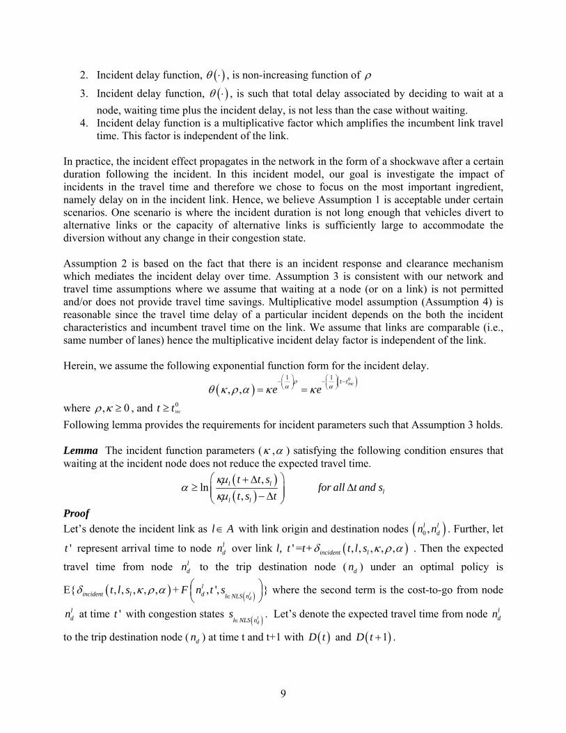
I.2. Preliminary Incident Delay Model Our incident delay function, ( )θ ⋅ , is based on incident severity (κ ), duration/stage ( ρ ), and

incident response (α ). Our incident delay model is a multiplicative model in that ( ), ,θ κ ρ α represents the factor by which the link travel time under same conditions (congestion state and link arrival time) is increased. Specifically, given the link travel time without incident, ( ), , lt l sδ and incident parameters (κ , ρ ,α ), the link travel time with incident is expressed as:

( ), , , , ,incident lt l sδ κ ρ α = ( ), ,θ κ ρ α ( ), , lt l sδ In the expected sense:

( ){ }, , , , ,incident lE t l sδ κ ρ α = ( ) ( ){ }, , , , lE t l sθ κ ρ α δ Note that incident duration/stage, ρ , depends on the duration between incident occurrence time ( 0

inct ) and arrival time to the link (t), i.e. { }0 0:inc inct t t tρ = − ≥ . We make the following assumptions for the incident function:

1. Incident delay is only experienced on the incident link (no propagating delay effect in the remainder of the network)

9

2. Incident delay function, ( )θ ⋅ , is non-increasing function of ρ

3. Incident delay function, ( )θ ⋅ , is such that total delay associated by deciding to wait at a node, waiting time plus the incident delay, is not less than the case without waiting.

4. Incident delay function is a multiplicative factor which amplifies the incumbent link travel time. This factor is independent of the link.

In practice, the incident effect propagates in the network in the form of a shockwave after a certain duration following the incident. In this incident model, our goal is investigate the impact of incidents in the travel time and therefore we chose to focus on the most important ingredient, namely delay on in the incident link. Hence, we believe Assumption 1 is acceptable under certain scenarios. One scenario is where the incident duration is not long enough that vehicles divert to alternative links or the capacity of alternative links is sufficiently large to accommodate the diversion without any change in their congestion state. Assumption 2 is based on the fact that there is an incident response and clearance mechanism which mediates the incident delay over time. Assumption 3 is consistent with our network and travel time assumptions where we assume that waiting at a node (or on a link) is not permitted and/or does not provide travel time savings. Multiplicative model assumption (Assumption 4) is reasonable since the travel time delay of a particular incident depends on the both the incident characteristics and incumbent travel time on the link. We assume that links are comparable (i.e., same number of lanes) hence the multiplicative incident delay factor is independent of the link. Herein, we assume the following exponential function form for the incident delay.

( ) ( )01 1

, ,inct t

e eρ

α αθ κ ρ α κ κ⎛ ⎞ ⎛ ⎞− − −⎜ ⎟ ⎜ ⎟⎝ ⎠ ⎝ ⎠= =

where , 0ρ κ ≥ , and 0inct t≥

Following lemma provides the requirements for incident parameters such that Assumption 3 holds. Lemma The incident function parameters (κ ,α ) satisfying the following condition ensures that waiting at the incident node does not reduce the expected travel time.

( )( )

,ln

,l l

ll l

t t sfor all t and s

t s tκμ

ακμ⎛ ⎞+ Δ

≥ Δ⎜ ⎟⎜ ⎟− Δ⎝ ⎠

Proof Let’s denote the incident link as l A∈ with link origin and destination nodes ( )0 ,l l

dn n . Further, let

't represent arrival time to node ldn over link l, 't =t+ ( ), , , , ,incident lt l sδ κ ρ α . Then the expected

travel time from node ldn to the trip destination node ( dn ) under an optimal policy is

E{ ( ), , , , ,incident lt l sδ κ ρ α + ( ), ', ld

ld l NLS n

F n t s∈

⎛ ⎞⎜ ⎟⎝ ⎠

} where the second term is the cost-to-go from node

ldn at time 't with congestion states ( )l

dl NLS ns∈

. Let’s denote the expected travel time from node ldn

to the trip destination node ( dn ) at time t and t+1 with ( )D t and ( )1D t + .

10

( ) ( ) ( ) ( ), , , , , , t+ , , , , , , ld

lincident l d incident l l NLS n

D t t l s F n t l s sδ κ ρ α δ κ ρ α∈

⎛ ⎞= + ⎜ ⎟⎝ ⎠

( ) ( ) ( ) ( )1 1, , , , 1, , t+1+ 1, , , , 1, , ld

lincident l d incident l l NLS n

D t t l s F n t l s sδ κ ρ α δ κ ρ α∈

⎛ ⎞+ = + + + + +⎜ ⎟⎝ ⎠

Assumption 3 states that at any node arrival time (t), waiting at the node does not lead to lower destination arrival time than without waiting. We write this condition for the minimal waiting time of 1 unit time.

( ){ } ( ){ }1 1E D t E D t+ − ≥ − We assume that cost-to-go functions alone satisfy this relationship as we assumed that link travel times (in both congestion states) are such that waiting at a node does not provide travel time savings. For unit waiting time this leads to the following relation for every t:

( ) ( ) ( ) ( ), t+1+ 1, , , , 1, , , t+ , , , , , , 1l ld d

l ld incident l d incident ll NLS n l NLS n

F n t l s s F n t l s sδ κ ρ α δ κ ρ α∈ ∈

⎛ ⎞ ⎛ ⎞+ + − ≥ −⎜ ⎟ ⎜ ⎟⎝ ⎠ ⎝ ⎠

Hence, we have the following relation: ( ){ } ( ){ }1, , , , 1, , , , , , 1incident l incident lE t l s E t l sδ κ ρ α δ κ ρ α+ + − ≥ −

where ( ){ } ( ) ( ){ }

( ) ( ){ }( ) ( )

0

0

1

1

, , , , , , , , ,

, ,

,

inc

inc

incident l l

t t

l

t t

l l

E t l s E t l s

e E t l s

e t s

α

α

δ κ ρ α θ κ ρ α δ

κ δ

κ μ

⎛ ⎞− −⎜ ⎟⎝ ⎠

⎛ ⎞− −⎜ ⎟⎝ ⎠

=

=

=

We obtain the following equivalent expression: ( ){ } ( ){ }

( ) ( ) ( )01 1

1, , , , 1, , , , , , 1

1, , 1inc

incident l incident l

t t

l l l l

E t l s E t l s

e e t s t sα α

δ κ ρ α δ κ ρ α

κ μ μ⎛ ⎞ ⎛ ⎞− − −⎜ ⎟ ⎜ ⎟⎝ ⎠ ⎝ ⎠

+ + − ≥ −

⎡ ⎤+ − ≥ −⎢ ⎥

⎢ ⎥⎣ ⎦

Note that ( )01

inct te α

⎛ ⎞− −⎜ ⎟⎝ ⎠ is increasing in α and decreasing in 0

inct t− and attains maximum level at 1. Hence, we can write the above requirement as:

( ) ( )1

1, , 1l l l le t s t sακ μ μ⎛ ⎞−⎜ ⎟⎝ ⎠

⎡ ⎤+ − ≥ −⎢ ⎥

⎢ ⎥⎣ ⎦

After some algebraic steps, we obtain the following relation ( )( )

1,ln

, 1l l

l l

t st s

κμα

κμ⎛ ⎞+

≥ ⎜ ⎟⎜ ⎟−⎝ ⎠

For arbitrary waiting time tΔ this condition becomes: ( )( )

,ln

,l l

l l

t t st s t

κμα

κμ⎛ ⎞+ Δ

≥ ⎜ ⎟⎜ ⎟− Δ⎝ ⎠

11

I.3. Illustrative Example -- Implementation of SDP Routing Algorithm under ATIS

Figure 1. Example network with 6 nodes and 10 links.

Consider a stylized network example with 6 nodes and 10 links in Figure 1. Links lengths are as shown on the graph. Note that we are using the following referencing for links l l

o dn nl where l

on and ldn are origin and destination nodes of link l, respectively.

We consider Node 1 as the origin node and Node 6 as the destination node of the trip. Velocities on the links follow stochastic non-stationary distributions which vary with the time of the day. Velocity data is sampled for every 15-minute interval and then linearly interpolated on a minute basis. Traffic state on each link is classified according to Congested (Uncongested) depending on whether the velocity is less (greater) than a cut of speed which is assumed 50 mph for all links. Our assumptions in this implementation are as follows (mostly consistent with Kim, 2003):

1. Traffic congestion on links can be at either of the two states: Uncongested and Congested 2. Links’ congestion state follow Markov process and evolve independent of each other. 3. Link velocities follow non-stationary normal distribution 4. Travel times follow normal distribution 5. Link travel times are calculated based on the link’s congestion state at the time of arrival 6. Acyclic network 7. No waiting at the nodes 8. Incidents take place on the links and affect link travel time of the corresponding link, i.e.,

no secondary shockwave affect on the remainder of the network 9. Travel cost is proportionate to the travel time 10. All links in the network are observed through traffic flow sensors

1

4

3

2

5 6

d12=7 mile

d13=4 mile

d14=8 mile

d34=4 mile

d25=6 mile

d35=8 mile

d45=6 mile

d46=7 mile

d56=1 mile

Link with Incident

12

Recall that the state vector in the previous section, ( ), ,n t SΩ , includes congestion states of all

links in the network, i.e., ( ) ( ) ( ) ( ){ }1 2 | |, ,..., AS t s t s t s t= . When no real-time information is used

then the state vector would be ( ),n tΩ and the trip planning problem becomes a static routing problem with time-dependent stochastic travel times. Including state of all network links in the state vector is computationally challenging due to exponentially increasing size of the state space. Therefore we include the states of links which are more important than the others. Specifically, given a node where a routing decision to be made, we include states of links (called current links) outgoing from that node and links that are successors of current links (called successor links). Next we define the following for exposition clarity. First, for nodes we define the following sets:

( )SN n : Successor Nodes Set of node n, i.e., set of nodes with incoming arc from node n

( )NCLS n : Current Links Set of node n, i.e., set of outgoing links from node n

( )NSLS n : Successor Links Set of node n, i.e., set of outgoing links from the successor nodes of node n Let Node Links Set of node n as ( ) ( ) ( ){ }NLS n NCLS n NSLS n= ∪ .

Following examples illustrate these sets ( )1 {2,3, 4}SN n = = , ( ) 12 13 141 { , , }NCLS n l l l= = , and

( ) 25 35 34 45 461 { , , , , }NSLS n l l l l l= = . Next, we define the following sets for links:

( )LSLS l : Successor Links Set of link l, i.e., set of outgoing links from the destination node of l

( )LPSLS l : Post-Successor Links Set of link l, i.e., set of outgoing links from the destination

nodes of all links ( )'l LSLS l∈ .

Following examples illustrate these sets ( ) 12 13 141 { , , }NCLS n l l l= = , ( )13 34 35{ , }LSLS l l l= , and

( )13 45 46 56{ , , }LPSLS l l l l= Note that for a given ( )l NCLS n∈ , ( ) ( )LPSLS l NSLS n⊆ . Furthermore, for given a link l A∈

and ( )0 ,l ldn n , the successor links set of link’s destination node is equivalent to the union of

successor and post-successor links set of the link l, i.e., ( ) ( ) ( ){ }ldNSLS n LSLS l LPSLS l= ∪ .

Our backward dynamic programming algorithm requires structuring a tree form (called stage tree) to implement stage-wise backward induction. To obtain the stage tree, we convert a given network such that at every stage there is one outgoing arc from any node. Therefore in a stage tree, a node can appear in multiple stages. Figure 2 illustrates the stage tree for the example network.

13

6

4

5

1

3

2

4

1

3

1

STAGE 1 STAGE 2 STAGE 3 STAGE 4

Figure 2. Illustration of stage tree for the example network in Figure 1.

Finally define ( )A k as the set of links at decision stage k. For instance,

( ) { }14 34 35 25 453 , , , ,A k l l l l l= = . We now provide our backward dynamic programming algorithm. I.3.A. The Algorithm We now provide the algorithm for recurring congestion. In the end of this section we describe the changes in this algorithm to accommodate for non-recurring congestion namely incidents that affect link travel time. Backward DP Algorithm for Dynamic Routing with Real-Time Information Step 1. Initializations • Initialize network ( ),G N A= , origin/destination nodes of links and trip, latest arrival time to

destination M, and successor nodes sets ( )SN n for n N∀ ∈ • Generate tree form of decision making stages for backward induction • Generate link lists for nodes and links • Generate ( )NCLS n and ( )NSLS n for n N∀ ∈

• Generate ( )LSLS l and ( )LPSLS l for l A∀ ∈ • Generate velocity distributions for all links • Set length of unit time period t • Interpolate velocity for each time unit t • Partition velocities into congestion states. Fit distributions for each congestion state, link, and

time and estimate distribution parameters such as mean and standard deviation • Set maximum link travel times, i.e. ( )max

,max , ,

ll lt s

t l sδ δ=

14

• Calculate latest arrival times ( maxnAT ) for each for n N∀ ∈ such that

( )( )

( )' maxmax max'

, '

minn nln SN n

l n n

AT AT δ∈≡

≤ − and maxdnAT M=

• Estimate the single step congestion state transition probabilities ( ), 1lT t t + by fitting bi-variate Gaussian distribution for every consecutive time-period velocity pair for l A∀ ∈ .

• Calculate steady state probabilities of congestion states l A∀ ∈ • Set probability tolerance parameter 610Probε −= Step 2. Backward Dynamic Program Step 2.a. For k=K to 1, Repeat \\ starting from the last stage

For ( )l A k∀ ∈ , Repeat \\ for link in the current stage

For 0kt t= to 0max

lnAT , Repeat \\ for every travel starting time on the current link

For ( ) {1, 2}l ks t = , Repeat \\ for every congestion state of the current link

For ( ) ( ) ( ){ }' {1, 2} 'l ks t l LSLS l LPSLS l= ∀ ∈ ∪ , Repeat \\ for every state

\\ prior to link l travel GoTo Step 2.b.

Set ( ) ( )( ) ( )( ) ( ) ( )( )( )0 0 0, , min , , | , , ,l l lk k k l k k kl NLS n l NLS nF n t s t F n t s t l F n t s t∈ ∈=

Set ( ) ( )( ) ( )( ) ( ) ( )( )0 0 0, , , , | , ,l l lk k k l k k kl NLS n l NLS nn t s t l if F n t s t l F n t s tπ ∈ ∈= ≤

Next ( )'l ks t

Next ( )l ks t

Next kt

Next l Next k

Step 2.b. Calculation of the cost-to-go for a given action ( )k kl π= Ω for the current state

( )( )0 , ,lk k l kn t s tΩ =

Set ( )( )0 , , |l

k l kF n t s t l :=0

For 1kδ = to ( )max

ldn

kAT t− , Repeat \\ for every travel time on link l

For ( ) ( ) ( ){ }' 1 {1, 2} 'l k k ks t t l LSLS l LPSLS lδ+ = + = ∀ ∈ ∪ , Repeat \\ for every state

\\ following link l travel

Calculate ( , , )k kg l δΩ where ( )( )0 , ,lk k l kn t s tΩ = \\ cost of travel on the current link l

Calculate ( )( )0P | , ,lk k l kn t s tδ \\ probability of travel time kδ on the current link l

Calculate ( ) ( )( ) ( ) ( ){ }' 'P | 'l k k l ks t s t l LSLS l LPSLS lδ+ ∀ ∈ ∪ \\ transition probabilities

15

If ( )( )0P | , ,lk k l k Probn t s tδ ε≤ or ( ) ( )( )' 'P |l k k l k Probs t s tδ ε+ ≤ , then Next kδ

Recall ( )( )', ,ld k k l k kF n t s tδ δ+ + \\ cost-to-go for the destination

\\ node of the current link l Calculate

( )( ) ( ) ( )( )( ) ( ){ }

( )( )

( )( )

0 ' ' 0'

'

, , | P | P | , ,

( , , )

, ,

l lk l k l k k l k k k l k

l LSLS l LPSLS l

k k k

ld k k l k k

F n t s t l s t s t n t s t

g l

F n t s t

δ δ

δ

δ δ

∈ ∪

⎡ ⎤+ = +⎢ ⎥

⎢ ⎥⎣ ⎦Ω⎡ ⎤

× ⎢ ⎥+ + +⎢ ⎥⎣ ⎦

∏

Next ( )'l ks t

Next kδ

Return to Step 2.a.

For the non-recurring congestion case we modify the above algorithm by there is an incident, we modify the step 2.b. of the above algorithm. We now illustrate the modification with a simple integration of incident information in the algorithm. Let’s assume that there is an incident on link

13l at the start of the trip. This incident brings about a delay in the travel time of link 13l . This incident delay (θ ) is a function of link(l), time(t), initial incident severity(κ ), incident stage( ρ ), i.e., ( ), , ,l tθ κ ρ . Here we assume that ( ), , ,l tθ κ ρ =θ =constant for this simple case. Then the step 2.b. of the previous algorithm is modified as below. Modification of Step 2.b. of the Backward DP Algorithm for Dynamic Routing with Real-Time Information and Incidents Step 2.b. Calculation of the cost-to-go for a given action ( )k kl π= Ω for the current state

( )( )0 , ,lk k l kn t s tΩ =

Set ( )( )0 , , |l

k l kF n t s t l :=0

For 1kδ = to ( )max

ldn

kAT t− , Repeat \\ for every travel time on link l

For ( ) ( ) ( ){ }' 1 {1, 2} 'l k k ks t t l LSLS l LPSLS lδ+ = + = ∀ ∈ ∪ , Repeat \\ for every state

following link l travel

Calculate ( , , )k kg l δΩ where ( )( )0 , ,lk k l kn t s tΩ = \\ cost of travel on the current link l

Calculate ( )( )0P | , ,lk k l kn t s tδ \\ probability of travel time kδ on the current link l

Calculate ( ) ( )( ) ( ) ( ){ }' 'P | 'l k k l ks t s t l LSLS l LPSLS lδ θ+ + ∀ ∈ ∪ \\ transition probabilities

If ( )( )0P | , ,lk k l k Probn t s tδ ε≤ or ( ) ( )( )' 'P |l k k l k Probs t s tδ θ ε+ + ≤ , then Next kδ

Recall ( )( )', ,ld k k l k kF n t s tδ θ δ θ+ + + + \\ cost-to-go for the destination node of the current

link l Calculate

16

( )( ) ( ) ( )( )( ) ( ){ }

( )( )

( )( )

0 ' ' 0'

'

, , | P | P | , ,

( , , )

, ,

l lk l k l k k l k k k l k

l LSLS l LPSLS l

k k k

ld k k l k k

F n t s t l s t s t n t s t

g l

F n t s t

δ θ δ

δ θ

δ θ δ θ

∈ ∪

⎡ ⎤+ = + +⎢ ⎥

⎢ ⎥⎣ ⎦Ω +⎡ ⎤

× ⎢ ⎥+ + + + +⎢ ⎥⎣ ⎦

∏

Next ( )'l ks t

Next kδ

Return to Step 2.a.

I.3.B. Computational Results We have implemented the algorithm in the previous section to the test problem and identified the optimal policies ( )( )*

0 01, ,t S tπ . The maximum trip time parameter M is set as M=50.

Accordingly the latest node arrival times are { }max 1,34, 25,35, 48,50nAT = . Trip start time is set at

0 1t = . We simulated the trip 1000 times for the starting state of ( ) { }0 1 1,1,1,1,1,1,1,1,1,1S t = = . Expected travel time is found to be 17.60 minutes with a standard deviation of 1 minute. Distribution of the travel time is illustrated in Figure 3.

Figure 3. Distribution of travel time with recurring congestion.

Note that there are six alternative paths from origin to destination node in Figure 1. As a result of this simulation, the following paths are chosen with the following frequencies. Path 1: {1 3 5 6→ → → }, Frequency=155 times Path 1: {1 3 4 6→ → → }, Frequency=559 times

Freq

uenc

y

Travel Time

17

Path 1: {1 3 4 5 6→ → → → }, Frequency=286 times Next, we have implemented the algorithm with an incident on link 13l at the start of the trip. We set the parameters such that this incident brings about a delay of θ =10 minutes in the travel time of link 13l . We solved the problem using the modified step 2.b. for incident delay and identified the optimal policies. Then we re-simulated the trip for another 1000 times with the same starting state. This time expected travel time is found as 18.33 minutes with a standard deviation of 0.74 minutes. Distribution of the travel time with incident delay is illustrated in Figure 4.

Figure 4. Distribution of travel time with non-recurring congestion.

As a result of this simulation, the following paths are chosen with the following frequencies. Path 1: {1 4 5 6→ → → }, Frequency=276 times Path 1: {1 4 6→ → }, Frequency=724 times Because of the incident induced delay, our algorithm identified alternative routed to avoid the link

13l .

I.4. Experimental Study Comparing Policies Generated by Alternative Scenarios In this section, we describe an experimental study to assess the effect of different assumptions in generating dynamic routing policies. We compare policies generated under the assumption of stochastic versus deterministic travel times, single congestion state versus two congestion states, and with incident information versus no incident information. For this study, we used the example network illustrated in the previous section with realistically simulated network parameters (link lengths and velocities). In what follows we first describe our network characteristics and the

Freq

uenc

y

Travel Time

18

process used to generate problem parameters. Then we present our performance comparisons for policies generated under different assumptions. I.4.A. Data Generation In our dynamic routing model, we require the following data to be generated:

1. Link lengths 2. Non-stationary distributions of link travel times (by congestion state) 3. Markov model for congestion states (time varying state transitions and long run

probabilities) For this experiment, we have labeled links of the example network as “Link #” and specified their lengths as follows:

Link 1: d12=13 miles Link 2: d13=10 miles Link 3: d14=17 miles Link 4: d34=8 miles Link 5: d25=12 miles Link 6: d35=15 mile Link 7: d45=8 mile Link 8: d56=19 mile Link 9: d46=26 mile

0 200 400 600 800 1000 1200 1400

45

50

55

60

65

70

75

Time of the day (in cumulative minutes)

Velo

city

Gen

erat

ing

Patte

rn (m

ph)

Velocity Pattern

Figure 5. Daily velocity pattern used to generate velocity data.

We have then created a daily velocity pattern to generate velocities. This pattern is shown in Figure 5 and it has three pronounced modes which represent daily travel demand on the network. The x-axis represents the time of the day in cumulative minutes, i.e., 450 on the x-axis corresponds to 07:30. Clearly, in the morning, afternoon, and evenings there is an increased traveler demand which increases the link capacity utilization and thus reduces the average speeds. We have used this velocity pattern to generate both uncongested and congested velocities. We assumed that the pattern in Figure 5 corresponds the average uncongested state velocity. The average congested state velocities are assumed at 60 % of the uncongested state velocities.

19

Using the above pattern, we have generated 60 velocity samples which correspond to 60 days. In each sample, the velocity is assumed to reside in a particular congestion state for a certain amount of time after entering that state. In order to model this, we used uniform distribution between 9 and 12 minutes of constant state. At the end of each constant state we sampled from a Bernoulli distribution (with probability 0.70 in uncongested and 0.30 in congested state) to determine the subsequent congestion state. This approach is realistic in the sense that congestion states are persistent in practice; once we enter a congestion state, we experience that state for a variable amount of time which is usually greater than a certain minimum. A portion of a daily sample of the generated velocities is illustrated in Figure 6.

Figure 6. Illustration of generated velocities from a sample (7:00-8:30 time period for a particular day sample).

In order to differentiate between the velocity patterns used for different links, we phased the velocity pattern over the network. The rationale is that recurring congestion is determined by the traveler demand and thus not all links of a network experience the same velocity pattern at the same time as traveler demand propagates on the network over time. In this implementation, we assumed that outgoing links from Node 1 (1,2,3) are followed by intermediate links (4,5,6,7) which are followed by the incoming links to Node 6 (8,9). The phasing interval is selected as 15 minutes. This phasing can be observed form Figure 7. Following the sample velocity generation, we have calculated time and link dependent cut-off speeds for congestion and uncongestion states. These cut-off speeds are illustrated in Figure 6. Note that we have extended the previously adopted approach of assuming a constant cut-off speed (i.e. 50 mph). This extension is necessary since different times in a day have different velocity averages thus a constant cut-off speed would lead to incorrect congestion state classifications.

420 440 460 480 500 52020

40

60

80Link Velocities - Link No:1

420 440 460 480 500 52020

40

60


420 440 460 480 500 52020

30

40

50


420 440 460 480 500 52020

40

60


420 440 460 480 500 52020

40

60


420 440 460 480 500 5200

20

40

60


420 440 460 480 500 52020

40

60


420 440 460 480 500 52020

40

60


420 440 460 480 500 5200

20

40


20

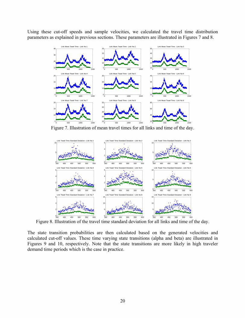
Using these cut-off speeds and sample velocities, we calculated the travel time distribution parameters as explained in previous sections. These parameters are illustrated in Figures 7 and 8.

0 500 1000 150010

20

30

40Link Mean Travel Time - Link No:1

0 500 1000 15005

10

15

20


0 500 1000 150010

20

30

40


0 500 1000 15005

10

15


0 500 1000 15000

10

20


0 500 1000 150010

20

30


0 500 1000 15005

10

15


0 500 1000 150010

20

30

40


0 500 1000 150020

40

60


Figure 7. Illustration of mean travel times for all links and time of the day.

350 400 450 500 550 6000

5

10Link Travel Time Standard Deviation - Link No:1

350 400 450 500 550 6000

2

4


350 400 450 500 550 6000

5


350 400 450 500 550 6000

2

4


350 400 450 500 550 6000

2

4


350 400 450 500 550 6000

5


350 400 450 500 550 6000

2

4


350 400 450 500 550 6000

5

10


350 400 450 500 550 6000

5

10


Figure 8. Illustration of the travel time standard deviation for all links and time of the day.

The state transition probabilities are then calculated based on the generated velocities and calculated cut-off values. These time varying state transitions (alpha and beta) are illustrated in Figures 9 and 10, respectively. Note that the state transitions are more likely in high traveler demand time periods which is the case in practice.

21

0 200 400 600 800 1000 1200 14000.55

0.6

0.65

0.7

0.75

0.8

0.85

0.9

0.95

1State Transition Probability (Congested-to-Congested)

Time of the day

Pro

babi

lity

Figure 9. State transition probabilities (α: congested state to congested state)

0 200 400 600 800 1000 1200 14000.7

0.75

0.8

0.85

0.9

0.95

1State Transition Probability (Uncongested-to-Uncongested)

Time of the day

Pro

babi

lity

Figure 10. State transition probabilities (β: uncongested state to uncongested state)

I.4.B. Performance Comparison of Alternative SDP Policies This section clearly illustrates the superior performance of the SDP derived dynamic routing policies when they accurately account for recurrent congestion (i.e., they differentiate between congested and uncongested states) and non-recurrent congestion attributed to incidents (e.g., accidents). First, we present results for the case where the network experiences no incidents but experiences recurrent congestion. Later, we present results for the case where the network is also experiencing non-recurring incidents besides recurrent congestion. Recurring Congestion In this case, the network is experiencing recurrent congestion but no incidents. We derive the dynamic routing policies in two ways. Initially, the SDP algorithm does not differentiate the congested state from the uncongested state, and models it as a single combined state in deriving an optimal policy, labeled a “single state policy”. Later, we allow the SDP algorithm to explicitly differentiate the two states (i.e., congested state from uncongested state) during policy development, leading to a “two state policy”. The two-state policy exploits the state information to dynamically route the vehicle.

22

Figure 11 presents the results for the case when the SDP algorithm does not differentiate the congested state from the uncongested state. Figure 12 presents the results for the case when the SDP algorithm does make an explicit distinction between the two states. It is very clear from the mean travel time plots that the two-state policy, explicitly accounting for recurrent congestion, yields more efficient routes (takes less time to complete the trip).

6:12 6:27 6:42 6:57 7:12 7:27 7:42 7:57 8:12 8:27 8:42 8:57 9:12 9:27 9:42 9:57

40

45

50

55

60

65

70

75

80

85

Mea

n Tr

avel

Tim

e

(a

ll co

nges

tion

stat

es)

Time of the day

Simulation of stochastic single-state policies with two-state traffic congestion

Figure 11. Mean travel times under single-state policy.

6:12 6:27 6:42 6:57 7:12 7:27 7:42 7:57 8:12 8:27 8:42 8:57 9:12 9:27 9:42 9:57 35

40

45

50

55

60

65

70

Mea

n Tr

avel

Tim

e

(a

ll co

nges

tion

stat

es)

Time of the day

Simulation of stochastic two-state policies with two-state traffic congestion

Figure 12. Mean travel times under two-state policy.

Recurring and Non-Recurring Congestion (Incidents) In this case, the network is experiencing both recurrent congestion as well as incidents. We derive the dynamic routing policies in two ways. Initially, the SDP algorithm does not account for on-line incident information. Later, we allow the SDP algorithm to explicitly account for on-line incident information to dynamically update the route. The results presented throughout the rest of this section pertain to incidents on link #6. In addition, the incidents are created on link #6 the same instant the vehicle departs the starting node. For example, if the vehicle departs the “starting or origin” node at 10AM, we create an incident on link #6 at 10AM as well. Given that link #6 is a downstream link (i.e., it is not connected to the origin node), by the time the vehicle reaches the incident link, the incident is partially cleared,

23

reducing the impact of the incident on link travel time. Due to space constraints, we are not presenting results from incidents on other links. The results from other links are very similar to those presented here. The incidents are created with different levels of “severity” and “clearance rate”. We report some of these results given the space constraints. Figures 13 and 15 present results for the case when the SDP algorithm does not account for on-line incident information, under different incident severity and clearance rates. Figures 14 and 16 present results for the case when the SDP algorithm does exploit on-line incident information. It is once again very apparent from these plots that the mean travel times are significantly reduced when the policy accounts for on-line incident information. Of course, the savings in travel time are a function of incident severity and clearance rates.

6:00 6:12 6:24 6:36 6:48 7:00 7:12 7:24 7:36 7:48 8:00 8:12 8:24 8:36 8:48 9:00 9:12 9:24 9:36 9:45 9:54

35

40

45

50

55

60

65

70

Mea

n Tr

avel

Tim

e

(a

ll co

nges

tion

stat

es)

Time of the day

Simulation of stochastic two-state policies with incident information

Figure 13. Mean travel times under two-state policy without accounting for incident information.

(Severity: κ =2; Response or Clearance Rate: α =7 (Fast))

6:00 6:12 6:24 6:36 6:48 7:00 7:12 7:24 7:36 7:48 8:00 8:12 8:24 8:36 8:48 9:00 9:12 9:24 9:36 9:45 9:5435

40

45

50

55

60

65

70

Mea

n Tr

avel

Tim

e (a

ll co

nges

tion

stat

es)

Time of the day

Simulation of stochastic two-state policies without incident information

Figure 14. Mean travel times under two-state policy while exploiting incident information.

(Severity: κ =2; Response or Clearance Rate: α =7 (Fast))

24

6:00 6:12 6:24 6:36 6:48 7:00 7:12 7:24 7:36 7:48 8:00 8:12 8:24 8:36 8:48 9:00 9:12 9:24 9:36 9:45 9:5435

40

45

50

55

60

65

70

75

Mea

n Tr

avel

Tim

e

(a

ll co

nges

tion

stat

es)

Time of the day

Simulation of stochastic two-state policies with incident information

Figure 15. Mean travel times under two-state policy without accounting for incident information.

(Severity: κ =2; Response or Clearance Rate: α =30 (Slow))

6:00 6:12 6:24 6:36 6:48 7:00 7:12 7:24 7:36 7:48 8:00 8:12 8:24 8:36 8:48 9:00 9:12 9:24 9:36 9:45 9:54

35

40

45

50

55

60

65

70

75

Mea

n Tr

avel

Tim

e

(a

ll co

nges

tion

stat

es)

Time of the day

Simulation of stochastic two-state policies without incident information

Figure 16. Mean travel times under two-state policy while exploiting incident information.

(Severity: κ =2; Response or Clearance Rate: α =30 (Slow)) Future experiments will study the differences between these different policies and scenarios in more detail.

I.5. Summary and Next Steps Over the course of this multi-year project, we first intend to relax many of the assumptions made by our current algorithms (e.g., allow traffic conditions on adjacent links to be correlated and not treat them to be independent). Subsequently, our goals (nor prioritized) are as follows:

• Extend the dynamic routing algorithms to account for: Cycles within the network, Incidents on distant links, and Travel within larger networks through modifications to stage tree construction procedure (that accounts for incoming links to origin node and outgoing links from destination node and existence of nodes and links not practically reachable from the point of origin).

• Methods for estimation of travel time (or cost) variance besides the expected travel time (or cost).

25

• Heuristics for computational/memory efficiency; In particular, our first preference here is to adapt the AO* algorithm for our needs. We are almost done with the implementation of the basic AO* algorithm. Future work will focus on improving the performance of AO* by developing smart and adaptive lower bounds. In addition, the focus will be on developing a variety of heuristics for computational/memory efficiency.

• Develop computationally efficient yet effective shockwave models that account for incident related traffic shockwaves propagating through nodes.

Our ultimate goal is to develop dynamic routing algorithms interfaced with real-time commercial GIS software that support constraints (e.g., user request to avoid local roads) and trips with multiple-legs (e.g., to support milk-run shipments). The validation studies will involve extensive testing of our models in the Southeast Michigan corridor. A key part of the validation would be to study the impact of these dynamic routing algorithms on the performance of Just-in-Time (JIT) deliveries to the three major Ford assembly plants (Michigan Truck, Wayne Assembly, and Dearborn Assembly) in Wayne County. Our collaborator, Ford’s MP&L, will be assisting us by providing data and statistics regarding freight delivery patterns/performance/costs between the facilities and the key JIT suppliers.

26

II: COLLABORATIONS WITH MITS-CENTER, METSIM, AND MDOT METRO REGIONS

II.1 Collaboration with MITS-Center and Traffic.com We have to date had multiple meetings with Mia Silver of MITS Center and her team to develop a better understanding for their traffic monitoring system (for southeast Michigan highways) and have also received some preliminary data representing several weeks of traffic for the southeast Michigan highways. We are currently in the process of analyzing this data to improve the quality of the models being developed for dynamic routing decision support when operating with access to ATIS (Advanced Traveler Information Systems) information. We had some preliminary discussions with Traffic.com and they have expressed their willingness to provide data for majority of high-ways in the Southeast-Michigan corridor. These datasets (and the networks resulting from them) will play a critical role for evaluating and refining our dynamic routing algorithms. Given that Traffic.com has been recently acquired by another company, the dataset delivery process has stalled. We are expecting a final word anytime now. Even if we do not receive these archive datasets, the MITS Center datasets will allow us to achieve all our objectives.

II.2 Collaboration with METSIM and MDOT Metro Region METSIM and Gateway projects, headed by Matt Webb of METSIM and Catherine Jensen at MDOT Metro Region, respectively, are two projects that aim to develop tools for strategic and operational planning of highway projects through micro-simulation models. Both of these projects are utilizing the Paramics Suite software package for traffic simulation. The METSIM model is nearly complete undergoing extensive calibration studies for simulation accuracy. The Gateway project extends the METSIM model to include major local roads in the Metro Region. Both Matt and Catherine are very supportive of our research efforts and plan to share nearly fully-specified micro-simulation models for the southeast Michigan corridor to test our dynamic routing decision models as well future analysis on the effect of traffic incidents (i.e. accidents, breakdowns) on the delivery reliability within JIT supply chain operations. While we are initially promised that both the METSIM model and the Gateway project model will be available by late summer, we are expecting delivery of these models by the end of the year. After consulting with Matt and Catherine and researching other traffic simulation software alternatives, we have decided to use Paramics for two reasons. First, it is versatile and allows us to incorporate our dynamic re-routing algorithms. Second, we will be able to use the traffic simulation models produced by the two projects. We have also been in contact with the company that provides Paramics Suite software. The software is relatively expensive, even for an academic license (priced between $5k and $10k depending on options). We are trying to identify other groups at Wayne State that might be interested in jointly purchasing a license.

27

III: RESULTS DISSEMINATION

III.1 Project Website We have established a Microsoft SharePoint Website for the project that helps us track/store all project related documents/information in one place. Currently, it carries all our literature, data sets, code, weekly research group meeting minutes, long-term mile-stones, short-term tasks, calendar, and contacts. While we currently control access to this website through password protection, we are in the process of opening parts of the website for anonymous access. The screen shots below highlight different parts of our website.

Homepage

Literature

Tasks

Meeting Minutes

28

III.2 Conference Activity Conference Presentations:

1. Guner, A., Chinnam, R.B., Murat, A., and Saripalle, M., “Enabling Congestion Avoidance in Stochastic Transportation Networks Under ATIS,” INFORMS 2007 Annual Meeting, Seattle (Nov 3-7, 2007).

2. Saripalle, M., Chinnam, R.B., Murat, A., and Guner, A., “Modeling Incidents for Dynamic Vehicle Routing Applications,” INFORMS 2007 Annual Meeting, Seattle (Nov 3-7, 2007).

3. Murat, A., Chinnam, R.B., Guner, A., Saripalle, M., and Azadian, F., “Dynamic Routing under ATIS for Congestion Avoidance,” Research Issues in Freight Transportation -- Congestion and System Performance Conference, Seattle (Oct 22-23, 2007).

Conference Sessions Organized:

1. We are organizing a special session titled “Urban Transportation Planning Models: Dynamic Routing with Real-time ITS Information” at the INFORMS 2007 Annual Meeting in Seattle (Nov 3-7, 2007) under the Cluster: Transportation Science & Logistics. The session is Chaired by our Co-PI – Dr. Alper Murat.

Conferences Attended:

1. Drs. Chinnam and Murat attended the Michigan Intelligent Transportation Systems Conference, May 16-17, 2007. Dr. Khasnabis, Associate Dean for Research College of Engineering has presented on our project along with other WSU efforts related to transportation.

2. Dr. Murat attended the Meeting Freight Data Challenges Conference, July 9–10, 2007 Renaissance Chicago Hotel, Chicago

Conferences Planning to Attend:

1. 2nd Annual National Urban Freight Conference- December 5-7, 2007 Long Beach, CA 2. TRB 87th Annual Meeting- January 13-17, 2008 Washington, DC

III.3 Journal Publications

A journal manuscript is being dispatched this week to the Computers & Operations Research journal that reports our SDP algorithms and their performance. A second manuscript based on the AO* algorithms is currently under preparation.

MI-OH UTC Project - Second Report from Chinnam at WSU...

Documents

Transcript of MI-OH UTC Project - Second Report from Chinnam at WSU...