Metso DNA Machine MonitoringMetso DNA ACN MR controller High performance modular rail mounted...

Machine condition

monitoring

Metso DNA Machine MonitoringOnline condition monitoring system for the mining and construction industry

Online machine condition monitoring is based on fixed installed sensors on the machinery, cabled into I/O stations where measurement data is collected and analyzed. Alarms are generated when preset alarm limits are exceeded. Fault diagnostic is performed with comprehensive signal analyzing tools. Defect development is monitored by tracking history trends, thereby providing the tools for predic-tive maintenance for scheduling services and action planning.Machine condition monitoring enables the detec-tion of machines that do not perform properly or have mechanical faults, such as:• bearing wear and instabilities• lubrication problems• unbalance• misalignment• thrust bearing wear• shaft defects• wear and looseness• gear mesh problems• resonances or impacts

Metso DNA Machine Monitoring measures and analyzes the mechanical condition and performance of machines, based on vibration measurements and other machine parameters. DNA Machine Monitoring provides both protec-tion and diagnostics tools for critical machinery, as well as condition monitoring and analyzing tools for predictive maintenance use. Online machine condition monitoring enables 24/7 monitoring, thus providing the fastest possible way to act on problems to secure plant avail-ability, protect assets, provide information for maintenance planning and increase working environment safety.

DNA Machine Monitoring can work as a fully integrated application in the Metso DNA auto-mation platform or as a stand-alone system.

Layered user interface from overall view into detailed analysis tools suits both for operator’s and predictive maintenance person’s use.

2 | Metso DNA Machine Monitoring

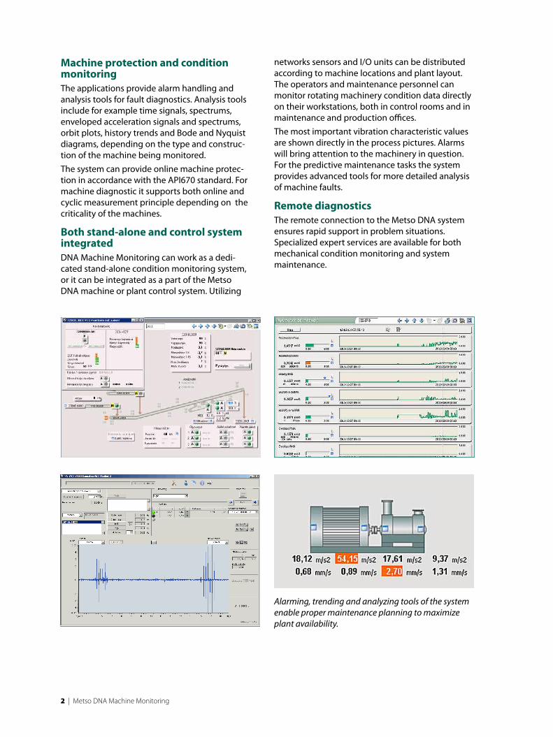
Machine protection and condition monitoringThe applications provide alarm handling and analysis tools for fault diagnostics. Analysis tools include for example time signals, spectrums, enveloped acceleration signals and spectrums, orbit plots, history trends and Bode and Nyquist diagrams, depending on the type and construc-tion of the machine being monitored.The system can provide online machine protec-tion in accordance with the API670 standard. For machine diagnostic it supports both online and cyclic measurement principle depending on the criticality of the machines.

Both stand-alone and control system integratedDNA Machine Monitoring can work as a dedi-cated stand-alone condition monitoring system, or it can be integrated as a part of the Metso DNA machine or plant control system. Utilizing

networks sensors and I/O units can be distributed according to machine locations and plant layout. The operators and maintenance personnel can monitor rotating machinery condition data directly on their workstations, both in control rooms and in maintenance and production offices. The most important vibration characteristic values are shown directly in the process pictures. Alarms will bring attention to the machinery in question. For the predictive maintenance tasks the system provides advanced tools for more detailed analysis of machine faults.

Remote diagnosticsThe remote connection to the Metso DNA system ensures rapid support in problem situations. Specialized expert services are available for both mechanical condition monitoring and system maintenance.

Alarming, trending and analyzing tools of the system enable proper maintenance planning to maximize plant availability.

Metso DNA Machine Monitoring | 3

DNA Machine Monitoring components

engineering and start-up services to training, system maintenance and condition analysis and reporting services.

Vibration and process sensorsReliability of the measurement data is ensured with sensors, connectors and cables designed for heavy and demanding industrial environments.

RVT105, acceleration sensor, low profile

RVT120, acceleration sensor, top exit

RTS-227, magnetic trigger sensor

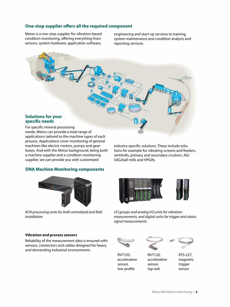
ACN processing units for both centralized and field installation

I/O groups and analog I/O units for vibration measurements, and digital units for trigger and status signal measurements

Solutions for your specific needsFor specific mineral processing needs, Metso can provide a total range of applications tailored to the machine types of each process. Applications cover monitoring of general machines like electric motors, pumps and gear-boxes. And with the Metso background, being both a machine supplier and a condition monitoring supplier, we can provide you with customized

industry-specific solutions. These include solu-tions for example for vibrating screens and feeders, vertimills, primary and secondary crushers, AG/SAG/ball mills and HPGRs.

Metso is a one-stop supplier for vibration-based condition monitoring, offering everything from sensors, system hardware, application software,

One-stop supplier offers all the required component

For more information, contact your local automation expert at Metso.

www.metso.com/automation

The information provided in this brochure contains descriptions or characteristics of performance which in case of actual use do not always apply as described or which may change as a result of further development of the products.

An obligation to provide the respective characteristics shall only exist if expressly agreed in the terms of contract. Availability and technical specifications are subject to change without notice.E8

974_

EN_0

1 1

2/20

12 ©

Met

so A

utom

atio

n In

c.

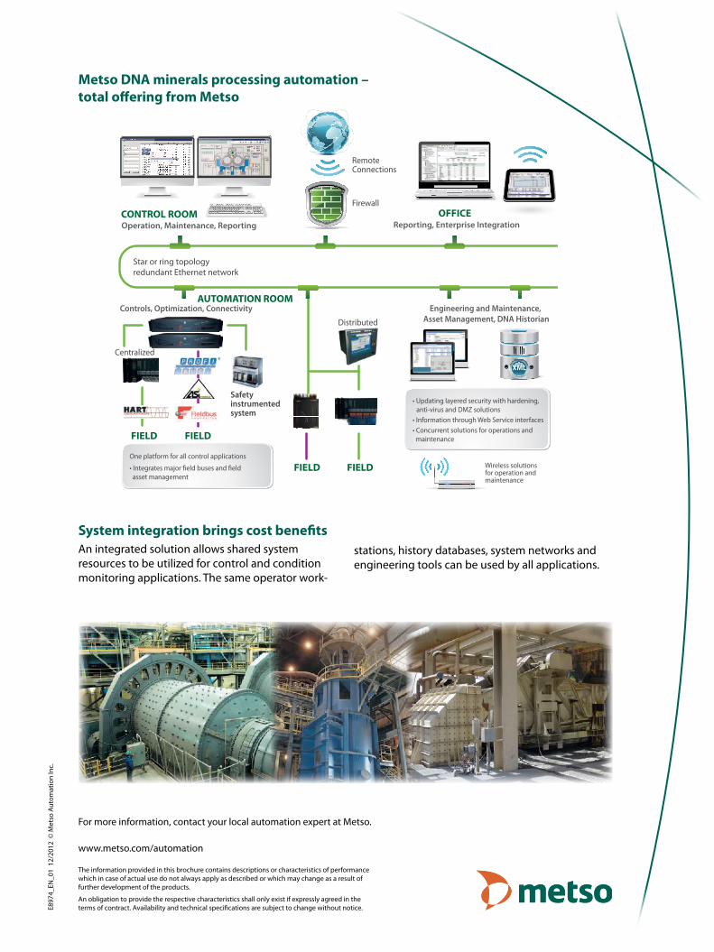
System integration brings cost benefitsAn integrated solution allows shared system resources to be utilized for control and condition monitoring applications. The same operator work-

stations, history databases, system networks and engineering tools can be used by all applications.

Metso DNA minerals processing automation – total offering from Metso

CONTROL ROOM

AUTOMATION ROOM

FIELDFIELD

FIELD FIELD

Operation, Maintenance, Reporting

Star or ring topology redundant Ethernet network

OFFICEReporting, Enterprise Integration

Engineering and Maintenance, Asset Management, DNA Historian

Controls, Optimization, Connectivity

Safety instrumented system

Centralized

Distributed

XML

Firewall

Remote Connections

• Updating layered security with hardening, anti-virus and DMZ solutions • Information through Web Service interfaces • Concurrent solutions for operations and maintenance

One platform for all control applications

• Integrates major field buses and field asset management

Wireless solutions for operation and maintenance

Metso D

NA

ACN MR controllerHigh performance modular rail mounted controller

ACN MR is a multi-functional controller and member of Metso DNA’s ACN controller family. The ACN MR controller is used in centralized, distributed and embedded applications. ACN MR can be also used in standalone applications with or without a connection to the Metso DNA system.

ACN MR is communication and application compatible with other ACN family control-lers and VME controllers.

Key features• Small size• High processing power• Advanced control features• Fast control cycles, down to 5 ms• No moving parts (fan or hard disk)• One-to-one redundancy capability• 5 x 100 Mbit/s Ethernet connections• Removable SD card

• G3 environmental specification with optional lacquered models

• Operating temperature 0...+70°C• Reliability due to the design and industrial compo-

nents• PROFIBUS DP interface unit (coming in 2013)• Serial interface unit (coming in 2013)

ACN MR installed on a mounting base and ACN M120 I/Os ACN MR installed on a mounting base and ACN M80 I/Os

2 |

100 Mbit/s

Control room

Engineering/Maintenanceserver

Information Managementserver

Router tooffice network

Extender

User Interface and Alarm Processor nodes

Ethernet network

ACN MR controllers in I/O cabinet

Metso DNA with ACN MR controllers

ACN MR structureThe ACN MR controller is installed on the mounting base (MBMT120 or MBMT80, depending of the ACN I/O product family) together with the power supply unit (IPSP).ACN MR mounting base can either be attached to the ACN I/O mounting bases with I/O units or ACN MR with power supply unit can be used as a sepa-rate controller.ACN MR has a removable SD card containing the parameters needed when a node is starting. If a spare node is taken in use, the SD card is unplugged and changed to a spare node and the spare node will boot with the same configuration as the original one.

In the typical configuration the real-time operating system (RTOS), Process Controller software and the application are loaded from the Backup Server when the node is starting.In standalone operation mode, software is loaded from local SD card. The SD card contains RTOS, Process Controller software and the application.

Architecture The ACN MR controller is scalable from applications with few I/Os to applications with several thousand I/Os. Because of the small physical size, ACN MR can be installed in the same cabinet with ACN I/Os.

Medium size and large size applicationsBelow is an example of a system with about 2500 I/Os. The system consists of three ACN I/O cabinets and control room nodes. Each ACN I/O cabinet has the ACN MR controller located at the top of the cabinet.

| 3

Distributed and small applications In distributed and small applications ACN MR controller is installed in the field cabinet with ACN I/O. Beside is a picture of a field cabinet with ACN MR and ACN I/O.

ACN MR process controllers and I/O in the field cabinet

InterfacesThe interfaces available in ACN MR are: • Four 10/100Base-T Ethernet ports on a CPU board

for:• communication with Metso DNA nodes• ACN I/O communication• Ethernet protocols like Modbus/TCP• serial communication via an Ethernet-serial

converter• One 1000Base-T Ethernet port for redundant

ACN MR• Three channel PROFIBUS DP interface unit and

two channel serial interface units are under development

RedundancyACN MR supports redundant Metso DNA Ethernet networks, redundant controllers (one-to-one redundancy) and redundant ACN I/O field buses and rack I/O.

Redundant ACN MR controllers and I/Os

I/O cabinet

I/O

I/O

I/OIBCIPSP

I/OIBCIPSP

I/OIBCIPSP

I/OIBCIPSP

I/OIBCIPSP

I/OIBCIPSP

ACN MRM

IPSP

IPSPACN MRR

IPSP

System busEthernetsingle/redundant

Ethernetswitch

Ethernet Field bus





859_

EN_0

3 1

1/20

12 ©

Met

so A

utom

atio

n In

c.

Performance• The number of I/O channels per ACN MR is typi-

cally 250...2000 with control cycles of 100...1000 ms.

• The minimum control cycle is 5 ms and maximum control cycle is 64 s

Dimensions [W x H x D] • ACNMR • MBMTmountingbase

40 x 125 x 95 mm 126 x 125 x 40 mm

Weight 1100g

Protection IP20

RAMmemory 512MB

Processor IntelAtom1.1GHz

SDcard 2GB

Ethernetports 5

USBports 2

Drives N/A

Expansion N/A

Operatingtemperature 0°C...+70°C

Storagetemperature -20°C...+70°C

G3environmentalspecificationwithoptionallacqueredunits

Powersupply 18...36VDC

Powerconsumption 10 W

Operatingsystem real-timeoperatingsystem

D201915 ACNMRNode

D201893 MBMT120–ACNMRmountingbaseforACNI/OM120

D202076 MBMT80–ACNMRmountingbaseACNI/OM80

D200989 Processcontrollerandgatewaybaselicense,pernode

D200990 ProcessControllerCapacityLicense/100I/Os

Technical specification• Compact rack mounted metal enclosure• Fanless structure, cooling implemented with heat

sinks

Licenses and hardware

Function block diagram

EngineeringThe engineering library of the ACN controller provides function blocks for controls at all levels, including basic process control, advanced quality, drives, and optimization controls. Fuzzy, MPC, and programmable function blocks are available as a standard.The Function Block CAD engineering tool is used for designing function block diagrams for process control loops, sequences, and interface applica-tions.Function block diagrams are saved in a common database located on the Engineering Server. At the same time, a function block diagram is a graphical document of an application, which is loaded in the runtime environment. This ensures that the docu-mentation is always up-to-date.

AIF8 161

Rev. 2

13 AIF8 (FAST ANALOG INPUT UNIT)AIF8V D201509AIF8T D201510

13.1 USEThe AIF8 units are eight--channel analog input units used to measure analog current andvoltage signals. The units are part of the ACNI/O M120product family. The measuringchan-nels of an AIF8 unit are galvanically connected but separated from the system per unit.

The AIF8 units can be used in Sensodec 6S and Metso DNA system for measurements inmechanical condition monitoring applications.

The AIF8V D201509 unit is for measuring 0...24 V voltage signals. The unit is equipped witha 4 mA constant current supply for acceleration sensors. The AIF8T D201510 unit is formeasuring the rotation speed signals from the synchronization sensors (for example,RTS--226). The unit is equipped with a channel--specific current--limited operating voltagesupply for the transmitter.

The measuring rangecan be selected and normalized programmatically. Analog RF and low--passfiltering aswell asprogrammatic digital filtering are carried out on the incomingsignals.

162 ACN I/O Units, M120 Series

Rev. 2

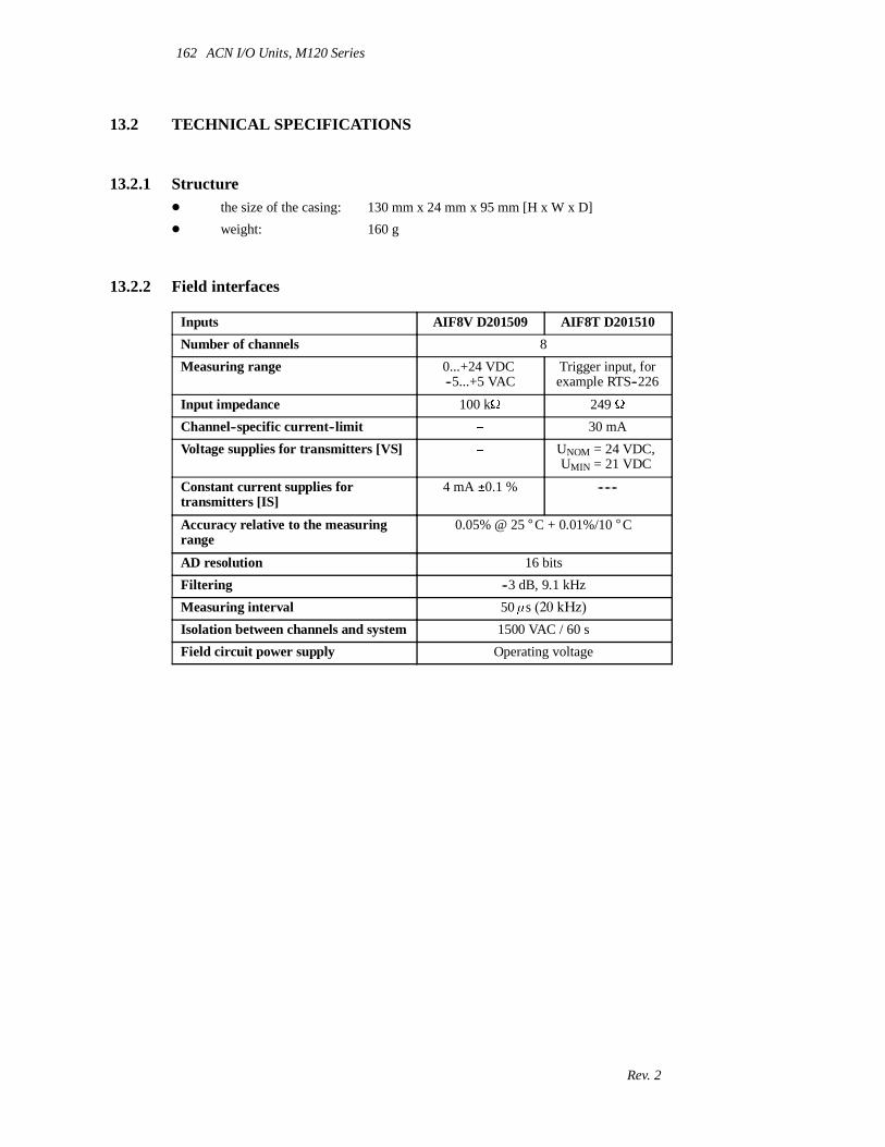
13.2 TECHNICAL SPECIFICATIONS

13.2.1 StructureD the size of the casing: 130 mm x 24 mm x 95 mm [H x W x D]D weight: 160 g

13.2.2 Field interfaces

Inputs AIF8V D201509 AIF8T D201510Number of channels 8Measuring range 0...+24 VDC

--5...+5 VACTrigger input, forexample RTS--226

Input impedance 100 k 249Channel--specific current--limit 30 mAVoltage supplies for transmitters [VS] UNOM = 24 VDC,

UMIN = 21 VDC

Constant current supplies fortransmitters [IS]

4 mA 0.1 % ------

Accuracy relative to the measuringrange

0.05% @ 25 °C + 0.01%/10 °C

AD resolution 16 bitsFiltering --3 dB, 9.1 kHzMeasuring interval 50 s (20 kHz)Isolation between channels and system 1500 VAC / 60 sField circuit power supply Operating voltage

AIF8 163

Rev. 2

13.3 ISOLATION

Field

Field

Field

Field

CH0

CH1

CH2

CH3Logic

= isolation 1500 VAC / 60 s

System potential

Field

Field

Field

Field

CH4

CH5

CH6

CH7

164 ACN I/O Units, M120 Series

Rev. 2

13.4 INPUT CIRCUITS

13.4.1 AIF8V

For the field cable connector of an AIF8V unit, the connection order for signals is as follows:

Channel AIF8V Pin0 COM (--) 10 IN / 4 mA (+) 21 COM (--) 31 IN / 4 mA (+) 42 COM (--) 52 IN / 4 mA (+) 63 COM (--) 73 IN / 4 mA (+) 84 COM (--) 94 IN / 4 mA (+) 105 COM (--) 115 IN / 4 mA (+) 126 COM (--) 136 IN / 4 mA (+) 147 COM (--) 157 IN / 4 mA (+) 16

For the cable connectors of an IXR16 cross connection board, the connection order for sig-nals is as follows:C = COM

Channel 7 7 6 6 5 5 4 4 3 3 2 2 1 1 0 0AIF8V IN C IN C IN C IN C IN C IN C IN C IN CIXR16 16 15 14 13 12 11 10 9 8 7 6 5 4 3 2 1

Machine condition

monitoring

Dual output acceleration and temperature sensorRVT/TT-125 Code: 600-10026Key features• Combined acceleration and temperature

measurement• Rugged design• Corrosion resistant• Hermetic seal• ESD protection• Reverse wiring protection• Top exit connector

RVT/TT-125 is an industrial accelerometer with internal temperature sensor. Dual output sensor is an optimal solution for condition monitoring applica-tions that utilize both vibration and temperature measurements.

RVT/TT-125 is suitable for machine monitoring in e.g. following industries:• Pulp and Paper• Mining and mineral industry• Power generation • Steel industry





967_

EN_0

1 0

9/20

12 ©

Met

so A

utom

atio

n In

c.

RVT/TT-125 specifications

Dynamic Sensitivity, ±5%, 25 °CAcceleration rangeAmplitude nonlinearityFrequency response ±10% ±3 dBResonance frequency, mounted, min.Transverse sensitivity, max.Temperature response

100 mV/g 80 g peak1% 1...7 000 Hz 0.5...12 000 Hz30 kHz5% of axial±10% (-25...+120 °C)

Temperature SensitivityTemperature measurement range

10 mV/°C +2... +120 °C

Electrical Power requirement Voltage source Bias currentOutput impedance, max.Bias output voltage, nominalGrounding

18...30 VDC 2...10 mA100 Ω12 VDCCase isolated, internally shielded

Environmental Temperature rangeVibration limitShock limit, min.Sealing

-50...+120 °C500 g5 000 gHermetic

Physical Sensing element designWeightCase materialMountingOutput connector Pin A Pin B Pin C

PZT ceramic, shear90 g316L stainless steelM8 integral stud, (6 Nm max. Torque)3 pin, MIL-C-5015 style Accelerometer signal/power Accelerometer and temperature sensor common Temperature sensor signal

Metso DNA

Machine Monitoring Operator Manual

Collection 2014 rev. 5 G2125_EN_05


ii

Metso Automation Inc. reserves the right to make changes in information contained in this publication without prior notice, and the customer should in all cases consult Metso Automation Inc. to determine whether any such changes have been made. This publication may not be reproduced and is intended for the exclusive use of Metso Automation Inc.'s customer.

The terms and conditions governing the sale of hardware products and the licensing and use of software products manufactured/delivered by Metso Automation Inc. consist solely of those set forth in the written contract between the Metso Automation Inc. and its customer. No statement contained in this publication, including statements regarding capacity, suitability for use, or performance of products, shall be considered a warranty for any purpose nor shall it be considered part of the contract or give rise to any liability of Metso Automation Inc.

In no event will Metso Automation Inc. be liable for any damages, including but not limited to incidental, indirect, special, or consequential damages (including lost profits), arising out of or relating to this publication or the information contained in it, even if Metso Automation Inc. has been advised, knew, or should have known of the possibility of such damages.

Software

The content of the software described in the documentation (”Metso software”) is subject to the copyright of Metso Automation Inc. and/or its licensors.

Metso software is subject to Metso Automation Inc.'s license agreement. Metso Automation Inc. prohibits the use of this software unless you have valid license agreement with Metso Automation Inc. By taking Metso software into use, you signify your acceptance of the said license agreement.

Metso software may include certain open source or other software originated from third parties subject to the GNU General Public License (GPL), GNU Library/Lesser General Public License (LGPL) and other additional copyright licenses, disclaimers and notices. The exact terms of GPL, LGPL and certain other licenses are provided to you with Metso software. Please refer to the exact terms of the GPL, LGPL and other licenses regarding your rights under said licenses.

Metso Automation Inc. will provide copies of certain open source software to you on a CD-ROM for a fee covering the costs of such distribution (media, shipping and handling) upon a written request to Metso Automation Inc.'s address below or email address [email protected] (Subject: Source code requests). This offer is valid for a period of 3 years from the date of distribution of Metso software by Metso Automation Inc.

In accordance with the provisions of the public licenses, all contributors (as defined in the public licenses), with respect to the open source software, hereby DISCLAIM (i) ALL WARRANTIES AND CONDITIONS, express and implied, including warranties or conditions of title and non-infringement, and implied warranties or conditions of MERCHANTABILITY and FITNESS FOR A PARTICULAR PURPOSE, and (ii) all liability for damages, including direct, indirect, special, incidental and consequential damages, such as lost profits. You hereby accept and agree to the foregoing disclaimers.

© Metso Automation Inc, 1988 - 2014. All rights reserved. Printed in Finland.

Microsoft®, Windows® and Windows Server® are registered trademarks of Microsoft Corporation in the United States and/or other countries.

Metso Automation Inc.,

P.O. Box 237, FIN-33101 Tampere, Finland Tel. +358 20 483 170, Telefax +358 20 483 171


Metso DNA

iii

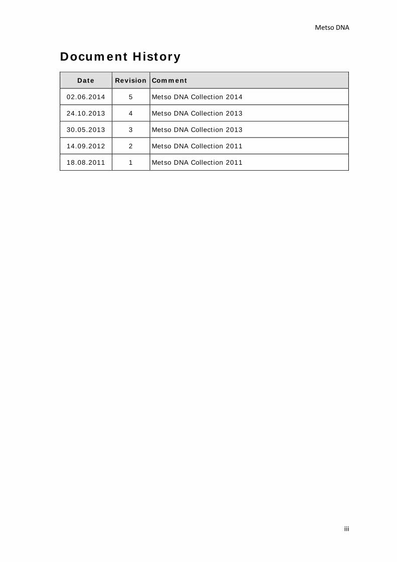
Document History

Date Revision Comment

02.06.2014 5 Metso DNA Collection 2014






iv

v

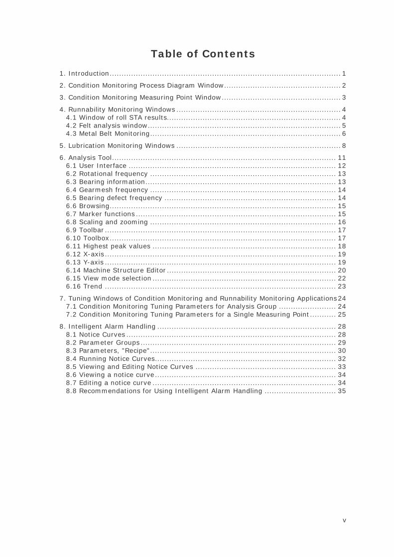
Table of Contents

1. Introduction ................................................................................................. 1

2. Condition Monitoring Process Diagram Window ................................................. 2

3. Condition Monitoring Measuring Point Window .................................................. 3

4. Runnability Monitoring Windows ..................................................................... 4 4.1 Window of roll STA results......................................................................... 4 4.2 Felt analysis window ................................................................................. 5 4.3 Metal Belt Monitoring ................................................................................ 6

5. Lubrication Monitoring Windows ..................................................................... 8

6. Analysis Tool .............................................................................................. 11 6.1 User Interface ....................................................................................... 12 6.2 Rotational frequency .............................................................................. 13 6.3 Bearing information ................................................................................ 13 6.4 Gearmesh frequency .............................................................................. 14 6.5 Bearing defect frequency ........................................................................ 14 6.6 Browsing ............................................................................................... 15 6.7 Marker functions .................................................................................... 15 6.8 Scaling and zooming .............................................................................. 16 6.9 Toolbar ................................................................................................. 17 6.10 Toolbox ............................................................................................... 17 6.11 Highest peak values ............................................................................. 18 6.12 X-axis ................................................................................................. 19 6.13 Y-axis ................................................................................................. 19 6.14 Machine Structure Editor ....................................................................... 20 6.15 View mode selection ............................................................................. 22 6.16 Trend ................................................................................................. 23

7. Tuning Windows of Condition Monitoring and Runnability Monitoring Applications 24 7.1 Condition Monitoring Tuning Parameters for Analysis Group ........................ 24 7.2 Condition Monitoring Tuning Parameters for a Single Measuring Point ........... 25

8. Intelligent Alarm Handling ........................................................................... 28 8.1 Notice Curves ........................................................................................ 28 8.2 Parameter Groups .................................................................................. 29 8.3 Parameters, "Recipe" .............................................................................. 30 8.4 Running Notice Curves ............................................................................ 32 8.5 Viewing and Editing Notice Curves ........................................................... 33 8.6 Viewing a notice curve ............................................................................ 34 8.7 Editing a notice curve ............................................................................. 34 8.8 Recommendations for Using Intelligent Alarm Handling .............................. 35

1

1. Introduction Machine Monitoring supervises the state of mechanical equipment and observes running stability. Monitoring is based mainly on vibration measurements and vibration characteristics derived from them. Warnings and alarms are issued to the user when characteristics limit values are exceeded. Time history of the vibration values can be observed through history trends of the calculated characteristics.

For a condition monitoring specialist, Machine Monitoring offers tools of analysis for investigating vibration signals and spectra as well as fault mechanisms. With the analysis tool, user can examine fault mechanisms and assess the severity of found mechanical faults.

In addition to mechanical measurements, a lubrication monitoring application that measures the oil flow of the circular lubrication and issues upper limit, lower limit and zero flow alarms as needed can also be included in the system.

With the tuning windows of the condition monitoring, application parameters can be changed directly in the user interface. These include alarm limits, scaling of graphical presentations, operating parameters of analysis cycles and storing cycles as well as calculation parameters of signal analysis.

2

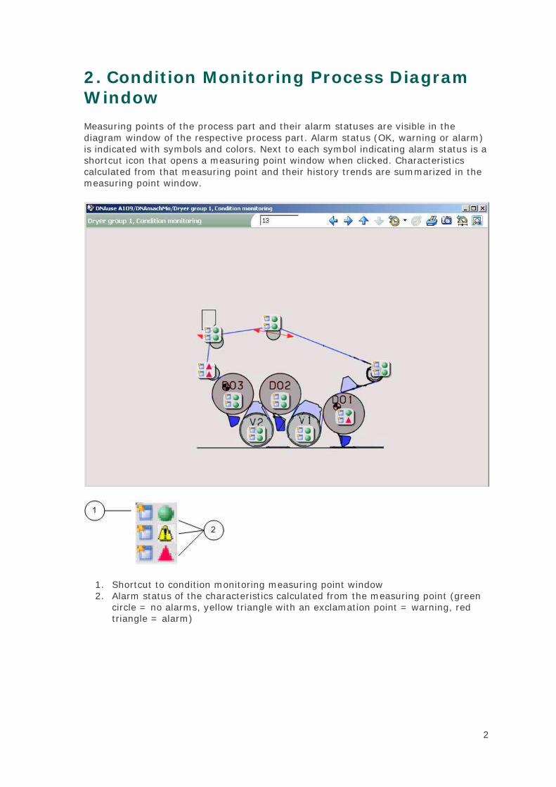
2. Condition Monitoring Process Diagram Window Measuring points of the process part and their alarm statuses are visible in the diagram window of the respective process part. Alarm status (OK, warning or alarm) is indicated with symbols and colors. Next to each symbol indicating alarm status is a shortcut icon that opens a measuring point window when clicked. Characteristics calculated from that measuring point and their history trends are summarized in the measuring point window.

1. Shortcut to condition monitoring measuring point window 2. Alarm status of the characteristics calculated from the measuring point (green

circle = no alarms, yellow triangle with an exclamation point = warning, red triangle = alarm)

3

3. Condition Monitoring Measuring Point Window Characteristics values calculated on the basis of measuring point, alarm limits, alarm status and history trends are displayed in the measuring point window. The window also includes a button for opening the analysis tool which is used by condition monitoring specialists for observing signals and spectra.

1. Starting analysis manually: performs measuring and updates results 2. Characteristics value as a number value and bar. Bar color indicates alarm

status (green, yellow, orange). The triangle above the bar points to the alarm limit.

3. History trend of the characteristics 4. Opens the analysis tool and fetches the vibration signal of the respective

measuring point.

4

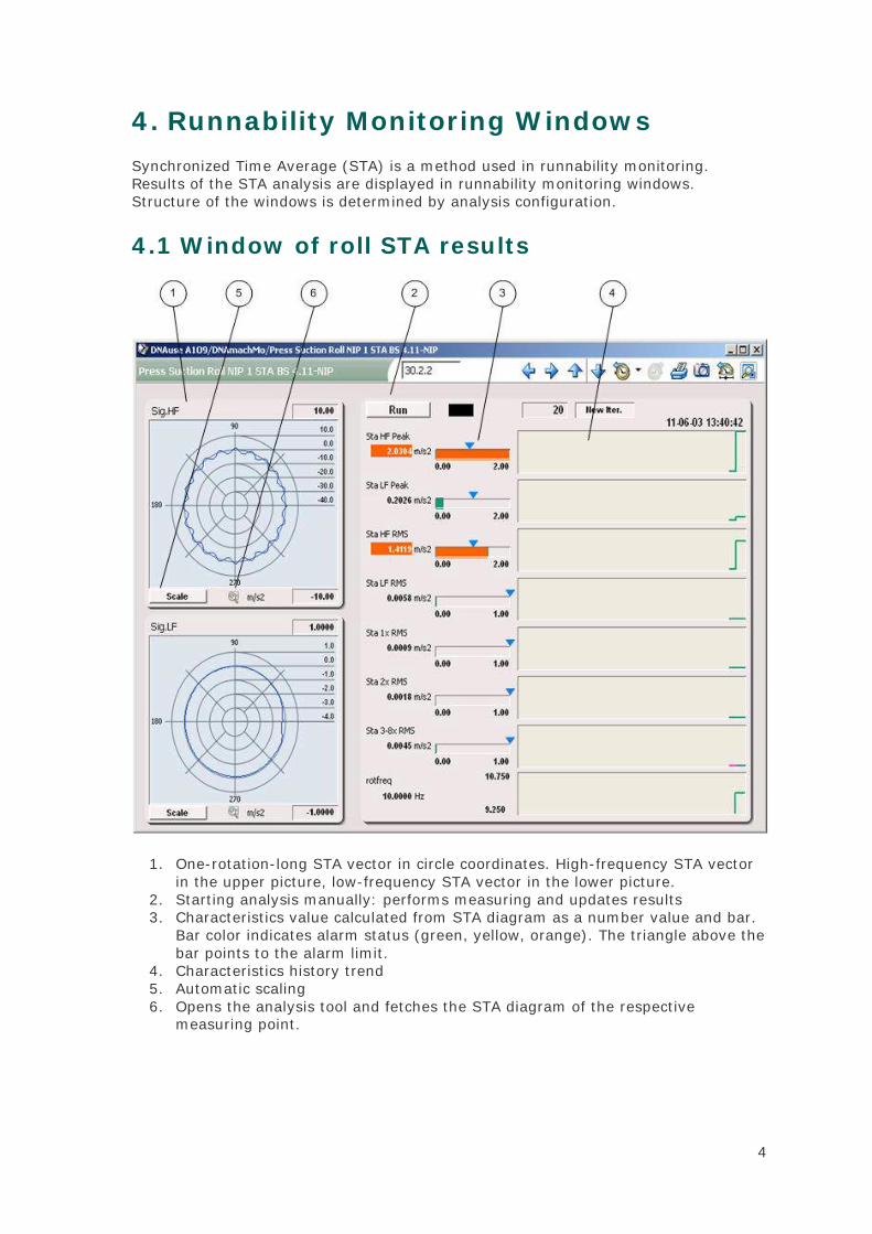
4. Runnability Monitoring Windows Synchronized Time Average (STA) is a method used in runnability monitoring. Results of the STA analysis are displayed in runnability monitoring windows. Structure of the windows is determined by analysis configuration.

4.1 Window of roll STA results

1. One-rotation-long STA vector in circle coordinates. High-frequency STA vector in the upper picture, low-frequency STA vector in the lower picture.

2. Starting analysis manually: performs measuring and updates results 3. Characteristics value calculated from STA diagram as a number value and bar.

Bar color indicates alarm status (green, yellow, orange). The triangle above the bar points to the alarm limit.

4. Characteristics history trend 5. Automatic scaling 6. Opens the analysis tool and fetches the STA diagram of the respective

measuring point.

Runnability Monitoring Windows

5

4.2 Felt analysis window

1. Starting analysis manually: performs measuring and updates results 2. Characteristics values calculated from nip vibration without synchronized

average ("raw signal") as number values and bars at the front and back side of nip rolls. Bar color indicates alarm status (green, yellow, orange). The triangle above the bar points to alarm limit.

3. Nip vibration characteristics values calculated from STA diagram as number values and bars at the front and back side of nip rolls. Bar color indicates alarm status (green, yellow, orange). The triangle above the bar points to alarm limit.

4. Characteristics history trend


6

4.3 Metal Belt Monitoring

Metal belt monitoring aims at predicting changes in the metal belt condition (used e.g. in ValZone), such as emerging cracks. The most essential measurements and calculations for belt monitoring are collected to the summary window.

Summary window:

1. Most important results of all five channels are displayed on the same page one below another.

2. First column shows the high frequency signal of the channels. 3. Second column shows the low frequency signal of the channels. 4. Third column shows the envelope signal of the channels. 5. Peak value of acceleration is calculated from the high frequency signal. 6. Peak counter is calculated from the envelope signal.

Open Peak Counter window using the button in the top right corner of the trend window:


7

1. Results of internal calculations of the block used in PeakCount calculation. 2. Tuning parameters of calculation. 3. PeakCount value calculated using the parameters. 4. RMS value calculated from the envelope signal. 5. Average of the envelope signal 6. Minimum value of the envelope signal 7. Maximum value of the envelope signal 8. Rotation frequency of the belt 9. Selection of calculation mode. The length of the data set used in PeakCount

calculation can be defined either as time or number of revolutions. 10. Length of calculation set (seconds/revolutions) 11. If two consecutive peaks are to be handled as a single peak, shutoff time can

be used to determine the time during which new peaks are not accepted. 12. Values exceedind the threshold are interpreted as peaks. The threshold can be

either an absolute acceleration value or a percentage of the RMS value of the envelope signal. (0 = absolute limits, 1 = percentage limits)

13. 14. Low and high threshold allow setting calculation of hysteresis value.

8

5. Lubrication Monitoring Windows User Interface of lubrication monitoring displays measuring stations of lubrication flow. When a station-specific symbol is clicked, a window opens with lubrication information of that station.

Lubrication monitoring user interface

Lubrication Monitoring Windows

9

Station-specific window

1. Manual update of station measuring results: reads station measurement values through a serial interface and updates results on screen.

Lubrication Monitoring Windows

10

2. Lubrication channel measurement value as a number value and bar. The line in the middle of the bar indicates lubrication flow setting value. Bar color indicates alarm status (green: normal, yellow: warning, orange: alarm, red: zero flow alarm). The lines above the bar show warning limits and the triangles point to alarm limits (upper and lower limits).

3. Opens a channel-specific settings window where the channel's monitoring application parameters, such as alarm limits, can be set. Password protected.

4. Opens the trend window of the respective lubrication channel.

11

6. Analysis Tool Machine Monitoring analysis tool is a versatile application designed for specialists for viewing closer spectra and time domain signals. The tool helps to identify developing mechanical faults, monitor machine function on a long term, and handle measured signals and spectra in many different ways.

User is provided with a wide range of marking, zooming and browsing functions, as well as shortcuts to facilitate usage.

Additionally, with user-specific settings, each user can modify tool functions and appearance to make usage more efficient and fluent.

Analysis Tool

12

6.1 User Interface

The user interface of the analysis tool consists of the following sections:

1. Rotational frequency 2. Bearing information 3. Gearmesh frequency 4. Bearing defect frequencies 5. Browsing 6. Marker functions 7. Scaling and zooming 8. Toolbar 9. Highest values 10. Resolution and frequency axis 11. Amplitude axis 12. Machine structure editor 13. View mode selection 14. Trend

Analysis Tool

13

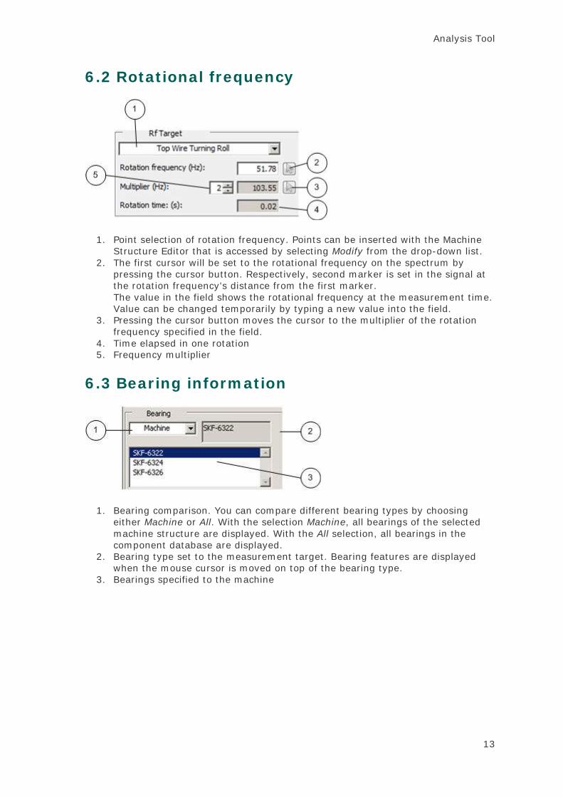
6.2 Rotational frequency

1. Point selection of rotation frequency. Points can be inserted with the Machine Structure Editor that is accessed by selecting Modify from the drop-down list.

2. The first cursor will be set to the rotational frequency on the spectrum by pressing the cursor button. Respectively, second marker is set in the signal at the rotation frequency's distance from the first marker. The value in the field shows the rotational frequency at the measurement time. Value can be changed temporarily by typing a new value into the field.

3. Pressing the cursor button moves the cursor to the multiplier of the rotation frequency specified in the field.

4. Time elapsed in one rotation 5. Frequency multiplier

6.3 Bearing information

1. Bearing comparison. You can compare different bearing types by choosing either Machine or All. With the selection Machine, all bearings of the selected machine structure are displayed. With the All selection, all bearings in the component database are displayed.

2. Bearing type set to the measurement target. Bearing features are displayed when the mouse cursor is moved on top of the bearing type.

3. Bearings specified to the machine

Analysis Tool

14

6.4 Gearmesh frequency

1. The first marker will be set to the gearmesh frequency on the spectrum by pressing the cursor button. The value in the field shows the frequency of the selected gearmesh in the measured rotational frequency.

2. Gearmeshes in the measured point. The gearmeshes can be inserted with the Machine Structure Editor.

6.5 Bearing defect frequency

1. The cursor can be moved to the frequency of bearing defect frequencies and frequency multiplier by pressing the cursor button. The values in the fields show bearing defect frequencies of the bearing type in the measured rotational frequency.

2. Ball spin frequency can be set to either base frequency or the second harmonic by clicking the button.

Analysis Tool

15

6.6 Browsing

1. Position selection, for browsing through all the positions on selected Process area. For quick browsing, the user can press arrow up and arrow down keys.

2. Result type selection, for example, Time level – Acceleration spectrum – Speed spectrum – Envelope time level – Envelope spectrum.

3. Button for Waterfall functions. 4. Serial number of the spectrum / total number of the saved spectra. Number 1

is the most recent and 1052 is the oldest. Click on the arrow buttons to move to the next measurement - to the left for a newer and to the right for an older.

5. Time point of the selected measurement. When opening the tool, the time point of the latest measurement is displayed. Measurements can be browsed also by selecting them directly from the Measurement time list.

6.7 Marker functions

Marker functions are located in two sections in the user interface, as described below.

Marker box

1. Active marker can be moved either by dragging the marker or by arrow buttons one step at a time. You can activate the marker by selecting the cursor with mouse or by clicking the selection box.

2. You can add markers by clicking the "+" button. 3. Marker coordinates on X- and Y-axes. 4. If the marker has been locked to the data, cursor movement follows the curve

points in steps according to the resolution. Opened lock means that movement of cursor is free and the steps for moving can be selected.

5. Frequency difference between two markers and time difference corresponding the frequency.

Analysis Tool

16

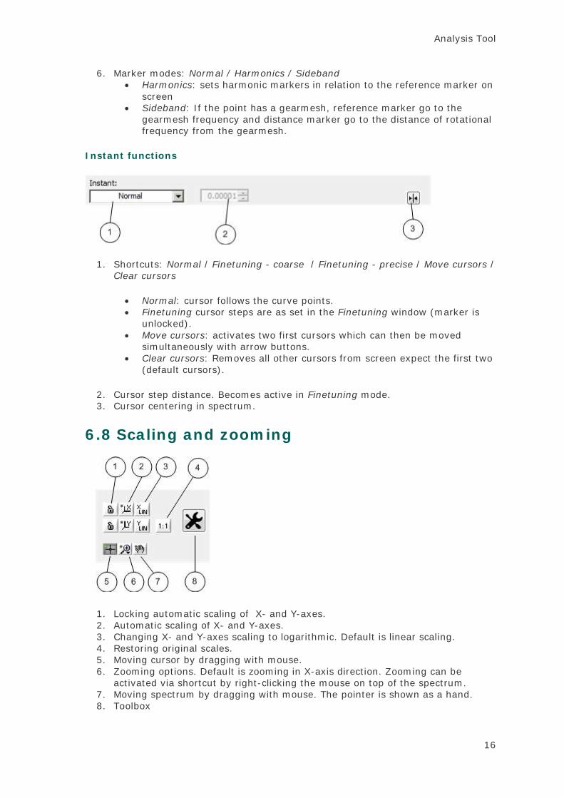
6. Marker modes: Normal / Harmonics / Sideband • Harmonics: sets harmonic markers in relation to the reference marker on

screen • Sideband: If the point has a gearmesh, reference marker go to the

gearmesh frequency and distance marker go to the distance of rotational frequency from the gearmesh.

Instant functions

1. Shortcuts: Normal / Finetuning - coarse / Finetuning - precise / Move cursors / Clear cursors

• Normal: cursor follows the curve points. • Finetuning cursor steps are as set in the Finetuning window (marker is

unlocked). • Move cursors: activates two first cursors which can then be moved

simultaneously with arrow buttons. • Clear cursors: Removes all other cursors from screen expect the first two

(default cursors).

2. Cursor step distance. Becomes active in Finetuning mode. 3. Cursor centering in spectrum.

6.8 Scaling and zooming

1. Locking automatic scaling of X- and Y-axes. 2. Automatic scaling of X- and Y-axes. 3. Changing X- and Y-axes scaling to logarithmic. Default is linear scaling. 4. Restoring original scales. 5. Moving cursor by dragging with mouse. 6. Zooming options. Default is zooming in X-axis direction. Zooming can be

activated via shortcut by right-clicking the mouse on top of the spectrum. 7. Moving spectrum by dragging with mouse. The pointer is shown as a hand. 8. Toolbox

Analysis Tool

17

6.9 Toolbar

Toolbar includes buttons for basic operations of Machine Monitoring.

1. User settings 2. Move window to the back of the screen 3. Information 4. Print

6.10 Toolbox

Toolbox is located in the right side of the Machine Monitoring user interface. Its functions depend on what is being examined. Options are Spectrum and Signal.

Spectrum

1. Restoring the original spectrum 2. Integration of the spectrum 3. Derivation of the spectrum 4. Freezing of the spectrum. If spectrum is not freezed after processing, it returns

to its original state when the toolbox is closed. 5. Automatic scaling of X- and Y-axes

Analysis Tool

18

Signal

1. Restoring the original signal 2. Rectification of the signal 3. Creating spectrum of the signal 4. Freezing the curve. If the curve is not freezed after processing, it returns to its

original state when the toolbox is closed. 5. Filter type selection (Low-pass, High-pass and Band-pass) 6. Cutoff frequency selection. Frequency can be changed by entering new values

to the input fields or dragging the indicators with mouse. You can also type the cutoff frequency scales. Default value is always 0-10 000 Hz.

6.11 Highest peak values

1. Highest value of the signal or three highest peaks of the spectrum. 2. The cursor will be set to the highest peak of the spectrum by pressing the

cursor button. 3. Peak-to-Peak value of the signal.

Analysis Tool

19

6.12 X-axis

1. Scale of X-axis. Scaling can be changed by typing new values. 2. Resolution of X-axis.

6.13 Y-axis

1. Scale of Y-axis. Scaling can be changed by typing new values. 2. Dimension of Y-axis.

Analysis Tool

20

6.14 Machine Structure Editor

Machine Structure Editor starts up when Modify is selected from the drop-down list above Machine Monitoring user interface Rotational frequency information.

With Machine Structure Editor, you can insert the bearing and gearmesh information of the item. This information can be directly utilized when analyzing measurement data in the analysis window. Below the Machine Structure Editor window:

Machine structure editor buttons:

1. Add new row 2. Edit selected row 3. Remove selected row 4. Save data 5. Set default value. Select a row that is displayed in the analysis window by

default when the tool is opened for this item.

Analysis Tool

21

Add new row

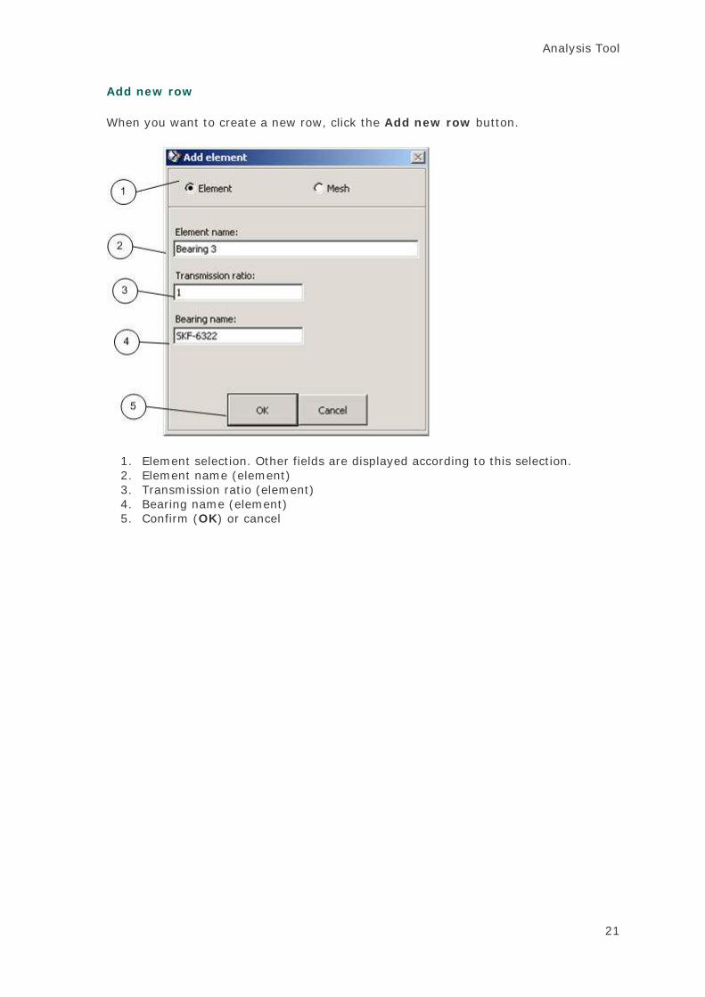
When you want to create a new row, click the Add new row button.

1. Element selection. Other fields are displayed according to this selection. 2. Element name (element) 3. Transmission ratio (element) 4. Bearing name (element) 5. Confirm (OK) or cancel

Analysis Tool

22

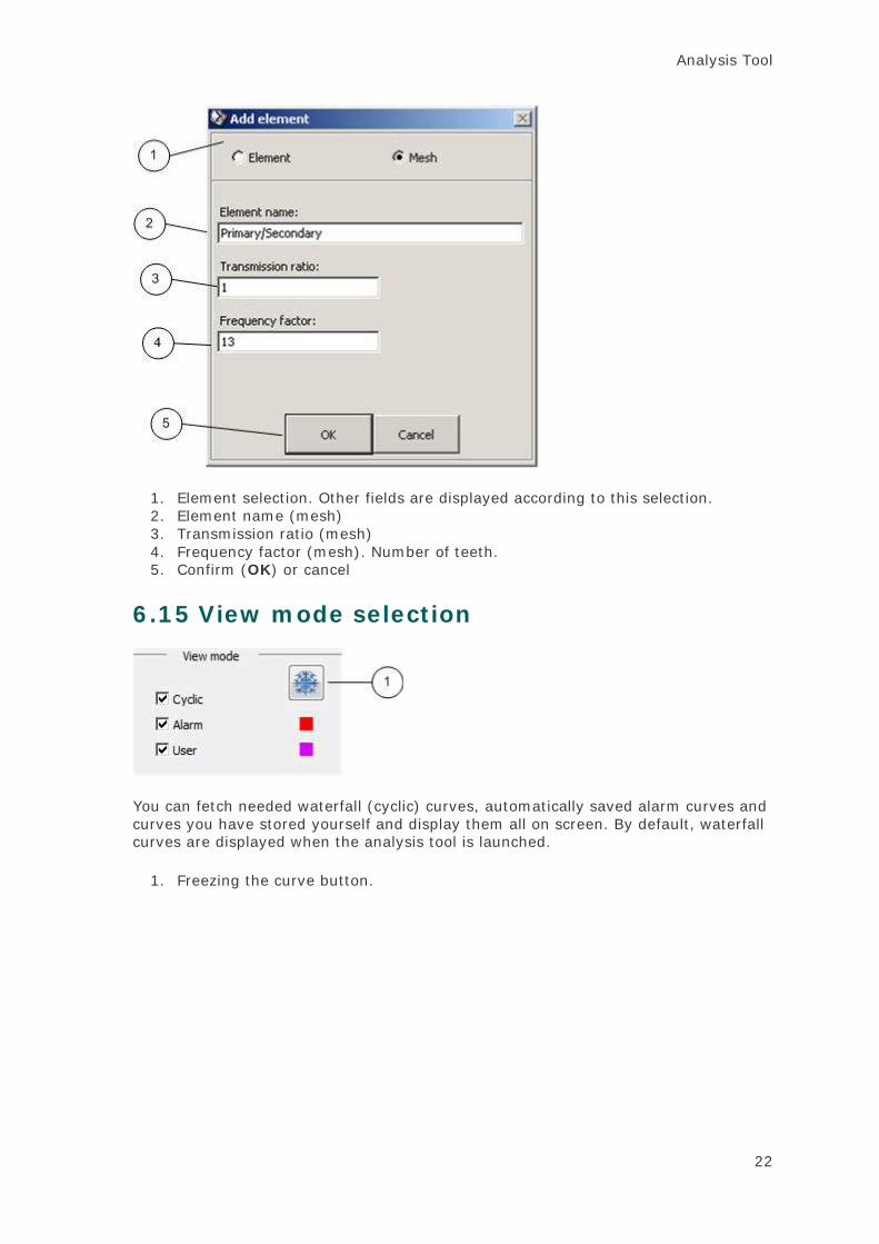
1. Element selection. Other fields are displayed according to this selection. 2. Element name (mesh) 3. Transmission ratio (mesh) 4. Frequency factor (mesh). Number of teeth. 5. Confirm (OK) or cancel

6.15 View mode selection

You can fetch needed waterfall (cyclic) curves, automatically saved alarm curves and curves you have stored yourself and display them all on screen. By default, waterfall curves are displayed when the analysis tool is launched.

1. Freezing the curve button.

Analysis Tool

23

6.16 Trend

You can browse machine trends by selecting a trend from the drop-down list and fetch trend point curves by dragging the cursor in the trend view. The same scaling and zooming functions are available as in the spectrum window. You can also select the length of the trend from the drop-down list.

24

7. Tuning Windows of Condition Monitoring and Runnability Monitoring Applications In tuning windows, parameters related to condition monitoring application can be altered, such as graphical presentation scaling, alarm and warning limits as well as analysis measurement parameters. Changes can be applied on two levels: either to the whole measuring point group or to a single measuring point. When applied to the whole measuring point group, the changes affect all measuring points that use the settings of that group.

7.1 Condition Monitoring Tuning Parameters for Analysis Group

Changing the group parameters affects all measuring points that use the settings of that parameter group:

1. General settings:

• Analysis interval: operation cycle of the application • Vector storing interval: for example, when value is 3, every third vector

in operating cycle is saved to the circular buffer of the waterfall storage. • Disable group: Passivating analysis

Tuning Windows of Condition Monitoring and Runnability Monitoring Applications

25

2. Diagram scaling settings:

• Sig.scale: scaling of signal drawing • EnvSig.scale: scaling of envelope signal drawing • IntegSpec.scale: scaling of velocity spectrum drawing • Spec.scale: scaling of acceleration spectrum drawing • EnvSpec.scale: scaling of envelope spectrum drawing

3. Characteristics-specific settings:

• Bar graph limit: bar scale settings. Gmin, Gmax = minimum and maximum limits of drawing scaling.

• Alarm limits: alarm and warning limit settings. GHH= alarm limit, GH= warning limit.

• Acceleration RMS characteristics: Band (Hz): RMS characteristics frequency band. GH= upper limit frequency, GL=lower limit frequency

• Velocity RMS characteristics: Band (Hz): RMS characteristics frequency band. GH= upper limit frequency, GL=lower limit frequency

• Vel.RMS m-nxRPM: Band (rpm): Frequency band upper and lower limit of the velocity RMS value that is calculated in relation to rotational frequency (GH= upper limit, GL= lower limit) for example, GH=20 and GL=5 -> frequency band is 5xRPM-20xRPM

• VelRMS TCxRPM: Band and TC: multiplier and bandwith parameters for velocity RMS value that is calculated in relation to rotational frequency. GTC= frequency multiplier, GBW= bandwidth around the monitored frequency. For example GTC= 25, GBW= 5 -> RMS value is calculated from a frequency band with center frequency of 25xRPM and bandwidth +/-5 percent of the center frequency.

• Envelope Peak: Filters Hz: Limit frequency values of band-pass filter and low-pass filter used in envelope analysis. GBpH= upper limit frequency of band-pass filter, GBpL= lower limit frequency of band-pass filter, GLpH= limit frequency of low-pass filter.

• Envelope RMS: Frequency band of RMS characteristics calculated from the envelope signal (GBpH= upper limit frequency, GBpL= lower limit frequency)

7.2 Condition Monitoring Tuning Parameters for a Single Measuring Point

Parameters of each measuring point can be set individually for that point, or parameters can be read from analysis group settings. The choice can be made for each parameter by selecting either L for individual setting of a measuring point or G for parameter group setting. If L is selected, group parameters do not affect that setting. If G is selected, local settings for that measuring point are not valid but group settings apply.


26

Tuning window for a single measuring point

1. Scaling settings of diagram drawing:

• For each setting, selection is made either for L= individual settings of the respective point, or G= settings are read from group settings

• Sig.scale: Scaling of signal drawing • EnvSig.scale: Scaling of envelope signal drawing • IntegSpec.scale: Scaling of velocity spectrum drawing • Spec.scale: Scaling of acceleration spectrum drawing • EnvSpec.scale: Scaling of envelope spectrum drawing

2. Characteristics-specific settings:

• L/G choice determines for each parameter whether group settings or individual settings are used. L= local settings of the specific setting are valid. G= settings are read from group settings

• Bar graph limit: bar scaling settings. Lmin, Lmax= lower and upper limits of an individual drawing; Gmin,Gmax= group limits; L/G selection determines whether group parameters or individual parameters are in use.

• Alarm limits: alarm and warning limit settings. LHH= individual alarm limit, LH= individual warning limit; GHH= group alarm limit, GH= group warning limit, IHH= speed-dependent alarm limit (individual), IH= speed-dependent warning limit (individual).


27

• Acceleration RMS characteristics: Band (Hz): Frequency band of RMS characteristics. GH= group upper limit frequency, GL= group lower limit frequency, LH= individual upper limit frequency, LL= individual lower limit frequency. L/G selection determines whether group parameters or individual parameters are in use.

• Velocity RMS characteristics: Band (Hz): Frequency band of RMS characteristics. GH= group upper limit frequency, GL= group lower limit frequency, LH= individual upper limit frequency, LL= individual lower limit frequency. L/G selection determines whether group parameters or individual parameters are in use.

• Vel.RMS m-nxRPM: Band (rpm:) Upper and lower limit of RMS value frequency band calculated in relation to rotational frequency. GH= group upper limit, GL= group lower limit, LH= individual upper limit, LL= individual lower limit. L/G selection determines whether group parameters or individual parameters are in use. For example GH=20 and GL=5 -> frequency band is 5xRPM-20xRPM.

• VelRMS TCxRPM: Band and TC: multiplier and bandwidth parameters for velocity RMS value that is calculated in relation to rotational frequency. GTC= group frequency multiplier, GBW= group bandwidth around the monitored group frequency. LTC= individual rotational frequency multiplier, LBW= individual bandwidth around the monitored frequency. For example, LTC= 25, LBW= 5 -> RMS value is calculated from a frequency band withcenter frequency of 25xRPM and bandwidth +/-5 percent of the center frequency.

• Envelope Peak: Filters Hz: Limit frequency values of band-pass filter and low-pass filter used in envelope analysis. GBpH= upper limit frequency of group band-pass filter,GBpL= lower limit frequency of group band-pass filter, GLpH= limit frequency of group low-pass filter. BpH= upper limit frequency of individual band-pass filter, BpL= lower limit frequency of individual band-pass filter, LpH= limit frequency of individual low-pass filter. L/G selection determines whether group parameters or individual parameters are in use.

• Envelope RMS: Frequency band of RMS characteristics derived from envelope signal. GBpH= group upper limit frequency, GBpL= group lower limit frequency, BpH= individual upper limit frequency, BpL= individual lower limit frequency. selection determines whether group parameters or individual parameters are in use.

28

8. Intelligent Alarm Handling Using Intelligent Alarm Handling makes the alarm handling easier, especially in the machines, in which driving speeds change a lot and values of characteristics change by driving speed. In addition to driving speed, the changing variable can be also rotational frequency. IAH is based on use of notice curves, which can also be used for the targets, whose speed changes only a little. The becoming notice curve is in this case more simple than in targets whose speed changes more.

Setting and using the notice curves replaces the traditional alarm handling, which is based on groups and is handled by scaling tool. It is possible to set own alarm level for each speed zone by notice curves in characteristic-specific way.

8.1 Notice Curves

Functions dealing with notice curves are opened from the Intelligent Alarm Handling button in DNA Operate user interface. With these functions it is possible to:

• create parameter groups for running notice curves and create a "running recipe"

• choose the characteristics and targets for the curve run • run the notice curves • remove the notice curves

Intelligent Alarm Handling

29

8.2 Parameter Groups

New parameter group is created or an existing group can be edited in Edit group window assuming that the group is not in use.

• Give a descriptive name to the new group. • You can give more information about the parameter group in the Comments

field. • Select the characteristics needed for the group in the selection box on the left.

Click the + button to add them. • To remove characteristics from a group, select them in the box on the right and

click the - button. • Save the new group or changes made to a group by clicking the Save button in

the upper right corner.


30

8.3 Parameters, "Recipe"

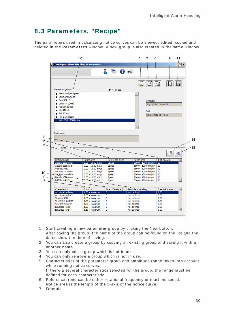
The parameters used in calculating notice curves can be viewed, edited, copied and deleted in the Parameters window. A new group is also created in the same window.

1. Start creating a new parameter group by clicking the New button. After saving the group, the name of the group can be found on the list and the dates show the time of saving.

2. You can also create a group by copying an existing group and saving it with a another name.

3. You can only edit a group which is not in use. 4. You can only remove a group which is not in use. 5. Characteristics of the parameter group and amplitude range taken into account

while running notice curves. If there a several characteristics selected for the group, the range must be defined for each characteristic.

6. Reference trend can be either rotational frequency or machine speed. Notice area is the length of the x-axis of the notice curve.

7. Formula.


31

8. Number of classes in the notice curve. Number of classes defines how many zones calculated separately there are in the notice curve. For example in this case the notice area is 0...60 Hz and there are 20 classes. The notice curve is divided into 20 parts of 3 Hz.

9. The maximum allowed in time difference between trend points. 10. If the class does not have any trend points during the selected time frame, the

value of the notice curve class can be defined. 11. Saving the parameter group. 12. The created parameter groups and the information on which groups are in use

= notice curves have been run using the parameter groups. 13. Copying the characteristic-specific parameters to all the characteristics of the

parameter group. 14. Editing the parameters.


32

8.4 Running Notice Curves

Targets and characteristics for the run of notice curves are selected in the Running notice curves window. Also the time frame from which the calculation data is used to create the notice curve is selected in this window.

1. Select the targets by first selecting the process, the machinery and characteristic in the selection boxes. You can select several items by holding the Ctrl or Shift button down while making the selection.

2. A parameter group contains the parameters needed for running the notice curves. To create a new group, click the Parameters button and give the group information in the window that opens.

3. You can set the length of the trends used in the calculation of notice curves either using the quick selection or freely.

4. Running the curves. 5. After deleting the notice curves the new results use normal alarm handling.


33

8.5 Viewing and Editing Notice Curves

Notice curves can be viewed and edited from the characteristic displays.

The "I" flag on the right side of the characteristic bar indicates that Intelligent Alarm Handling is in use in this characteristic.

You can view the notice curve by clicking the button under the "I" flag.


34

8.6 Viewing a notice curve

Notice curve created during the run can be viewed in the Viewing a notice curve window as a step-shaped curve and the measurement results as points.

1. Notice curve 2. Trend points 3. Used parameter group and the name of the target 4. Parameters 5. The time frame of the visible measurement results can be changed using the

quick selection or freely. 6. Editing the curve 7. Information on the notice curve 8. Markers

8.7 Editing a notice curve

1. You can edit the value of a single zone by dragging on the handle with the mouse.

2. You can add a new class (zone) into the beginning or end of the area. 3. Saving the changes. 4. Deleting the notice curve.


35

8.8 Recommendations for Using Intelligent Alarm Handling

In order to get all the benefits of Intelligent Alarm Handling and to have reliable results, the application should be used as systematically as possible. One possible way to use it in the paper machine environment is presented below.

1. Intelligent alarm handling is used only for machines and devices in good condition. Machine condition is checked beforehand and if there are trend points from defect situations, the points are removed from notice curve run using trend definition.

2. A few parameter groups are created, for example three for different rotational frequency ranges: one for large rolls, one for small rolls and one for motors and primary shafts. Rotational frequency ranges are determined from the measurement results so that the minimum limit of notice curve run is 1 Hz below the lowest and maximum limit is 1 Hz above the highest running speed. The frequency range is divided into 10...15 classes. The idea of the division is that the notice curve opens to the screen in the right scale without scaling and the speed changes are considered in the notice curve with sufficient accuracy.

3. Amplitude range can be defined high enough for the groups, according to possible maximum. Each notice curve is individual and a more accurate estimate is therefore not necessary.

4. The most important characteristics are included in the parameter groups, for example high frequency signal peak value (PEAK-HF) and RMS value of velocity spectrum (RMS-LF). Later on, after more experience, new parameter groups can be created for other characteristics.

5. Notice curves are run in appropriate batches, for example one process section at a time.

6. Notice curves are checked and, if necessary, the zones are edited directly using the editing handles.


36

Metso DNA Machine MonitoringMetso DNA ACN MR controller High performance modular rail mounted...

Documents

Transcript of Metso DNA Machine MonitoringMetso DNA ACN MR controller High performance modular rail mounted...