Metropolitan Land Values and Housing Productivitygroups.haas.berkeley.edu/realestate/seminars/Papers...

Metropolitan Land Values and Housing

Productivity∗

David Albouy

University of Michigan and NBER

Gabriel Ehrlich

University of Michigan

September 26, 2012

∗We would like to thank participants at seminars at the AREUEA Annual Meetings(Chicago), Ben-Gurion University, the Federal Reserve Bank of New York, the Housing-Urban-Labor-Macro Conference (Atlanta), Hunter College, the NBER Public EconomicsProgram Meeting, the New York University Furman Center, the University of BritishColumbia, the University of Connecticut, the University of Michigan, the University ofRochester, the University of Toronto, the Urban Economics Association Annual Meetings(Denver), and Western Michigan University for their help and advice. We especially wantto thank Morris Davis, Andrew Haughwout, Albert Saiz, Matthew Turner, and WilliamWheaton for sharing data, or information about data, with us. The National Science Foun-dation (Grant SES-0922340) generously provided financial assistance. Please contact theauthor by e-mail at [email protected] or by mail at University of Michigan, Departmentof Economics, 611 Tappan St. Ann Arbor, MI.

Abstract

We present the first nationwide index of directly-measured land values by metropoli-

tan area and investigate their relationship with housing prices. Construction prices

and geographic and regulatory constraints are shown to increase the cost of housing

relative to land. On average, approximately one-third of housing costs are due to

land, with an increasing share in higher-value areas, implying an elasticity of sub-

stitution between land and other inputs of about one-half. Conditional on land and

construction prices, housing productivity is relatively low in larger cities. The in-

crease in housing costs associated with greater regulation appears to outweigh any

benefits from improved quality-of-life.

JEL Codes: D24, R1, R31, R52

1 Introduction

Housing is the largest expenditure item for most households, yet the price of hous-

ing appears to vary widely depending on where it is located. This price variation

appears to come largely from differences in underlying land values, which can vary

tremendously according to the access land provides to local amenities and employ-

ment. Because they embody the value of location itself, land values are possibly

the most fundamental prices examined in urban economics.

Accurate data on land values have been notoriously piecemeal. Although data

on housing values are widespread and are often used in their place, the two are not

perfect substitutes: housing and land values can differ for several reasons. First, the

labor and material costs of producing housing structures may vary geographically.

Second, the topographical nature of a land parcel’s terrain can influence the quanti-

ties of inputs needed to produce housing structures. Third, regulations on land use

can raise expensive barriers to building, lowering the efficiency with which housing

services are provided and creating what is often referred to as a “regulatory tax.”

While these regulations may be costly, they may also provide external benefits to

neighboring residents. Whether land-use regulations are on net welfare improving

is perhaps the most hotly debated issue in the microeconomics of housing.

Here, we provide the first inter-metropolitan index of directly-observed land val-

ues that covers a large number of American metropolitan areas, using recent data

from CoStar, a commercial real estate company. On its own, this index measures

aggregate differences in the value of amenity, employment, and building opportuni-

ties across metros, encapsulating their overall desirability. Furthermore, this index

varies far more than a similarly constructed index of housing values; the two in-

1

dices are strongly but imperfectly correlated, with important deviations we believe

are informative. With these two indices and data on non-land input prices, geogra-

phy, and regulation, we use duality methods (Fuss and McFadden 1978) to estimate

a cost function for housing services.

Our analysis provides a new measure of local productivity in the housing sector,

which we infer from the difference between the observed price of housing and the

cost predicted by land and other input prices. This productivity metric is a summary

indicator of how efficiently housing inputs are transformed into valuable housing

services within a metropolitan area. It also indicates local productivity in sectors

that produce goods not traded across cities. This measure may be contrasted with

measures of productivity in tradeables sectors, as in Beeson and Eberts (1989) and

Albouy (2009), and local quality of life, as in Roback (1982) and Gyourko and

Tracy (1991).

Using recent measures by Gyourko, Saiz, and Summers (2008) and Saiz (2010),

we investigate how local housing productivity is influenced by natural and artificial

constraints to development arising from geography and regulation. Our supply-

side approach to valuing housing, based on input prices and housing productivity,

strongly complements the demand-side approach to studying housing prices, based

on local amenities and employment. For instance, it allows us to determine whether

higher housing prices due to regulation are due to increases in demand or to re-

ductions in supply: the former raise land values and welfare, while the latter lower

them.

We find that, on average, approximately one-third of housing costs are due to

land: this share ranges from 11 to 48 percent in low to high-value areas, implying

2

an elasticity of substitution between land and other inputs of about 0.5 in our base-

line specification. Consistent estimation of these parameters requires controlling

for regulatory and geographic constraints: a standard deviation increase in aggre-

gate measures of these constraints is associated with 8 to 9 percent higher housing

costs. We also examine disaggregated measures of regulation and geography and

find that approval delays, supply restrictions, local political pressure, and state court

involvement predict the lowest productivity levels, although our estimates are im-

precise.

Overall, housing productivity differences across metro areas are large, with a

standard deviation equal to 23 percent of total costs, with 22 percent of the variance

explained by observed regulations. Contrary to assumptions in the literature (e.g.

Rappaport 2007) that productivity levels in tradeables and housing are the same, we

find the two are negatively correlated. For example, the San Francisco Bay Area

is very efficient in producing tradeable output, but very inefficient in producing

housing. In general, we find housing productivity to be decreasing, rather than in-

creasing, in city size, suggesting that there are urban diseconomies of scale in hous-

ing production. Additionally, we find that lower housing productivity associated

with land-use regulation is correlated with a higher quality of life, suggesting that

households may value the neighborhood effects these regulations promote. How-

ever, these effects are smaller than the welfare costs of lower housing productivity,

implying that regulations are inefficient on average.

Our transaction-based measure differs from common measures of land values

based on the difference between a property’s entire value and the estimated value

of its structure only. Davis and Palumbo (2007) employ this “residual” method suc-

3

cessfully across metro areas, although as the authors note, “using several formulas,

different sources of data, and a few assumptions about unobserved quantities, none

of which is likely to be exactly right.” Moreover, the residual method attributes

higher costs due to inefficiencies in factor usage – possibly from geographic and

regulatory constraints – to higher land values. This may explain why Davis and

Palumbo often find higher costs shares of land than we do.1

A few studies have examined data on both housing and land values. Rose (1992)

acquires data across 27 cities in Japan and finds greater geographic land availability

is associated with lower land and housing values. Ihlanfeldt (2007) takes assessed

land value measures from tax rolls in 25 Florida counties, and finds that land-use

regulations are associated with higher housing prices but lower land values. Glaeser

and Gyourko (2003) use an augmented residual method to infer land values, and

find that housing and land values differ most in heavily regulated environments.

Glaeser, Gyourko, and Saks (2005b) find that the price of units in Manhattan multi-

story buildings exceeds the marginal cost of producing them, attributing the dif-

ference to regulation. They argue the cost of this regulatory tax is larger than the

externality benefits they consider, mainly from preserving views.

The econometric approach we use differs in that it explicitly incorporates a cost

function, which models land as a variable input to housing production. This ap-

proach has similarities to Epple, Gordon, and Sieg (2010), who use separately as-

sessed land and structure values for houses in Alleghany County, PA, and find land’s

1Although hedonic methods can theoretically provide estimates of land values from housingvalues, these estimates can be questioned. Using an augmented residual method based on hedonics,Glaeser and Ward (2009) estimate a value of $16,000 per acre of land in the Greater Boston area,while presenting evidence that the market price of an acre is approximately $300,000 if new housingcan be built on it. They attribute this discrepancy to zoning regulations.

4

cost share to be 14 percent. We depend on variation across, rather than within cities,

so that our cost structure is also identified from variation in construction prices, ge-

ography, and a wide array of regulations. Unlike Epple et al. and Thorsnes (1997),

who uses data from Portland, our estimated elasticity of substitution between land

and non-land inputs is less than one, which is consistent with much of the older

literature – see McDonald (1981) for a survey – based on data within cities

Three recent papers also make use of the CoStar COMPS data to construct land-

value indices. Haughwout, Orr, and Bedoll (2008) construct a land price index for

1999 to 2006 throughout the New York metro area, demonstrating the land data’s

extensive coverage. Kok, Monkkonen, and Quigley (2010) also document land

sales throughout the San Francisco Bay Area, and relate the sales prices to the

topographical, demographic, and regulatory features of the site. Nichols, Oliner,

and Mulhall (2010) construct a panel of land-value indices for 23 metro areas from

the 1990s through 2009. They demonstrate that land values vary more across time

than housing values, much as our analysis demonstrates is true across space.

Section 2 presents our cost-function approach for modeling housing prices and

relates it to an econometric model. It also provides a general-equilibrium model

for the full determination of land values. Section 3 discusses our data and explains

how we use them to construct indices of land values, housing prices, construction

prices, geography, and regulation across metro areas. Section 4 presents our esti-

mates of the housing-cost function and how housing productivity is influenced by

geographic and regulatory constraints. Section 5 considers how housing productiv-

ity varies across cities and is related to measures of urban productivity in tradeables

and quality of life.

5

2 Model of Land Values and Housing Production

Our econometric model uses a cost function for housing production embeded within

a general-equilibirum model of urban systems, proposed by Roback (1982), and

developed by Albouy (2009). The national economy contains many cities indexed

by j, which produce a numeraire good, X , traded across cities, and housing, Y ,

which is not traded across cities, and has a local price, pj . Cities differ in their

productivity in the housing sector, AjY .

2.1 Cost Function for Housing

We begin with a two-factor model in which firms produce housing, Yj , using land

L and materials M according to the production function

Yj = F Y (L,M ;AYj ), (1)

where F Yj is concave and exhibits constant returns to scale (CRS) in L andM at the

firm level. Housing productivity, AYj , is a city-level characteristic that may be fixed

or determined endogenously by city characteristics, such as population size. Land

is paid a city-specific price, rj , while materials are paid price vj . In our empirical

work, we operationalize M as the installed structure component of housing, so vj is

conceptualized as an index of construction input prices, e.g. an aggregate of local

labor and mobile capital. Unit costs in the housing sector, equal to marginal and

average costs, are cY (rj, vj;AYj ) ≡ minL,M{rjL+ vjM : FY (L,M ;AY

j ) = 1}.2

2The use of a single function to model the production of a heterogenous housing stock is wellestablished in the literature, beginning with Muth (1960) and Olsen (1969). In the words of Eppleet al. (2010, p. 906), “The production function for housing entails a powerful abstraction. Houses

6

Assuming the housing market in city j is perfectly competitive3, then in equi-

librium housing price equals the unit cost in cities with positive production:

cY (rj, vj;AYj ) = pj. (2)

Our methodology of estimating housing productivity is illustrated in figure 1A,

holding vj constant. The thick solid curve represents the cost function of hous-

ing for cities with average productivity. As land values rise from Denver to New

York, housing prices rise, albeit at a diminishing rate, as housing producers substi-

tute away from land as a factor input. The higher, thinner curve represents the cost

function for a city with lower productivity, such as San Francisco. The lower pro-

ductivity level is identified by how much higher the housing price in San Francisco

is relative to a city with the same factor costs, such as in New York.

The first-order log-linear approximation of equation (2) around the national av-

erage expresses how housing prices should vary with input prices and productivity,

pj = φLrj + (1 − φL)vj − AYj . zj represents, for any z, city j’s log deviation

from the national average, z, i.e. zj = ln zj − ln z. φL is the cost share of land

are viewed as differing only in the quantity of services they provide, with housing services beinghomogeneous and divisible. Thus, a grand house and a modest house differ only in the numberof homogeneous service units they contain.” This abstraction also implies that a highly capital-intensive form of housing, e.g., an apartment building, can substitute in consumption for a highlyland-intensive form of housing, e.g., single-story detached houses. Our analysis uses data fromowner-occupied properties, accountiing for 67% of homes, of which 82% are single-family anddetached.

3Although this assumption may seem stringent, the empirical evidence is consistent with perfectcompetition in the construction sector. Considering evidence from the 1997 Economic Census,Glaeser et al. (2005b) report that “...all the available evidence suggests that the housing productionindustry is highly competitive.” Basu et al. (2006) calculate returns to scale in the constructionindustry (average cost divided by marginal cost) as 1.00, indicating firms in the construction industryhaving no market power. This seems sensible as new homes must compete with the stock of existinghomes. If markets are imperfectly competitive, then AY

j will vary inversely with the mark-up onhousing prices above marginal costs.

7

in housing at the average, and AjY is normalized so that a one-point increase in AY

j

corresponds to a one-point reduction in log costs.4 Rearranged, this equation infers

home-productivity from how high land and material costs are relative to housing

costs:

AjY = φLrj + (1− φL)vj − pj. (3)

If housing productivity is factor neutral, i.e., F Y (L,M ;AYj ) = AY

j FY (L,M ; 1),

then the second-order log-linear approximation of (2), drawn in figure 1B, is

pj = φLrj + (1− φL)vj +1

2φL(1− φL)(1− σY )(rj − vj)2 − AY

j , (4)

where σY is the elasticity of substitution between land and non-land inputs. This

elasticity of substitution is less than one if costs increase in the square of the factor-

price difference, (rj − vj)2. The actual cost share is not constant across cities, but

is approximated by

φLj = φL + φL(1− φL)(1− σY )(rj − vj), (5)

and thus is increasing with rj − vj when σY < 1. Our estimates of AYj assume that

a single elasticity of substitution describes production in all cities. If this elasticity

varies, then our estimates will conflate a lower elasticity with lower productivity.

This is seen in figures 1A and 1B, which compare σY = 1 in the solid curves, with

σY < 1 in the dashed curves. When production has low substitutability, the cost

curve is flatter, as housing does not use less land in higher-value cities. This has the

4This normalization makes productivity at the national average obey AY =−p/[∂cY (r, m, AY )/∂A].

8

same observable consequence of increasing housing prices, although theoretically

the concepts are different.5

If housing productivity is not factor neutral, then as derived in Appendix A,

equation (4) contains additional terms to account for the productivity of land relative

to materials, AY Lj /AYM

j :

−φL(1− φL)(1− σY )(rj − vj)(AY Lj − AYM

j ). (6)

If σY < 1, then cities where land is expensive relative to materials, i.e., rj > vj , see

greater cost reductions where the relative productivity level, AY Lj /AYM

j , is higher.

2.2 Econometric Model

As a starting point, we estimate housing prices using an unrestricted translog cost

function (Christensen et al. 1973) in terms of land and non-land factor prices:

pj = β1rj + β2vj + β3(rj)2 + β4(vj)

2 + β5(rj vj) + Zjγ + εj, (7)

where Zj is a vector of city-level observable attributes that may affect housing

prices. This specification is equivalent to the second-order approximation of the

cost function (see, e.g., Binswager 1974, Fuss and McFadden 1978) under the re-

5Housing supply, as a quantity, is less responsive to price increases when substitutability is low,rather than when productivity is low. While it would be desirable to distinguish the two, this wouldbe significantly more challenging and require much additional data, and so we leave it for futurework.

9

strictions imposed by CRS

β1 = 1− β2, β3 = β4 = −β5/2, (8)

where φL = β1 and, with factor-neutral productivity, σY = 1 − 2β3/ [β1(1− β1)].

Housing productivity is determined by attributes in Zj and unobservable attributes

in the residual, εj:

AjY = Zj(−γ) + Aj

0Y , Aj0Y = −εj. (9)

The second-order approximation of the cost function (i.e. the translog) is not a

constant-elasticity form. Hence, the elasticity of substitution we estimate is evalu-

ated at the sample mean parameter values (see Griliches and Ringstad 1971). The

assumption of Cobb-Douglas (CD) production technology imposes the restriction

σY = 1, which in equation (7) amounts to the three restrictions:

β3 = β4 = β5 = 0. (10)

Without additional data, non-neutral productivity differences are impossible to

detect unless we know what may shift AY Lj /AYM

j . In the context, it seems rea-

sonable to interact productivity shifters Zj with the difference in input prices (rj−

νj) in equation (7). The reduced-form model allowing for non-neutral productivity

shifts, imposing the CRS restrictions may be written as:

pj − vj = β1(rj − vj) + β3[(rj)

2 + (vj)2 − 2(rj vj)

]+ γ1Z

j + γ2Zj (rj − vj) + εj

(11)

As shown in Appendix A, γ2Zj/2β3 = (AYMj − AY L

j ) − (AYM0j − AY L

0j ) identifies

10

observable differences in factor-biased technical differences. If σY < 1, then γ2 > 0

implies that the shifter Z lowers the productivity of land relative to the non-land

input.6

2.3 Full Determination of Land Values

In this section, we determine land values and local-wage levels in a model of loca-

tion demand based on amenities to households, bundled as quality of life, Qj , and

to firms in the tradeable sector, bundled as trade productivity, AXj . Casual read-

ers may skip this section without loss of intuition. We posit two types of mobile

workers, k = X, Y , where type-Y workers work in the housing sector. Preferences

are modeled by the utility function Uk(x, y;Qkj ), which is quasi-concave over con-

sumption x and y, increasing in Qkj , and varies by type. The household expenditure

function is ek(p, u;Q) ≡ minx,y{x + py : Uk (x, y;Q) ≥ u}. Each household

supplies a single unit of labor and is paid wkj,, which with non-labor income, I ,

makes up total income mkj = wk

j + I , out of which federal taxes, τ(mkj ), are paid.

We assume households are mobile and that both types occupy each city. Equilib-

rium requires that households receive the same utility in all cities, so that higher

prices or lower quality-of-life must be compensated with greater after-tax income,

ek(pj, uk;Qk

j ) = mkj − τ(mk

j ), k = X, Y, where uk is the level of utility attained

nationally by type k. Log-linearizing this condition around the national average

Qkj = sky pj − (1− τ k)skww

kj , k = X, Y. (12)

6In equation (11), non-neutral productivity implies β1 = φL + β3(AYM0j − AY L

0j ) and εj =

−[φLAY Lj + (1− φL)AYM

j ] + (1/2)φL(1− φL)(1− σY )(AY Lj − AYM

j )2

11

Qkj is normalized Qk

j is equivalent to a one-percent drop in total consumption, sky

is the average expenditure share on housing, and τ k is the average marginal tax

rate, and skw is the share of income from labor. Define the aggregate quality-of-life

differential Qj ≡ µXQXj + µY QY

j , where µk is the share of income earned by type

k households, and let sy ≡ µXsXy +µY sYy , and (1− τ) sww ≡ µX(1−τX)sXw wXj +

µY (1− τY )sYwwYj .

Unlike housing output, tradeable output has a uniform price across all cities,

and is produced through the CRS and CD function, Xj = FX(LX , NX , KX ;AXj ),

where NX is labor and KX is mobile capital, which also has the uniform price, i,

everywhere. We also assume that land in the same city commands the same price,

rj , in both sectors. A derivation similar to the one for (3) yields the measure of

tradeable productivity:

AXj = θLrj + θN wX

j , (13)

where θLand θN are the average cost-shares of land and labor in the tradeable sector.

To complete the model, let non-land inputs be produced through the CRS and

CD function Mj = (NY )a(KY )1−a, which implies vj = awYj , where a is the cost-

share of labor in non-land inputs. Defining φN = a(1 − φL), we can derive an

alternative measure of housing productivity based on wages:

AYj = φLrj + φN wY

j − pj. (14)

Combining the productivity in both sectors, the total-productivity differential of a

city is

Aj ≡ sxAXj + syA

Yj , (15)

12

where sx is the average expenditure share on tradeables.

Combining the first-order approximation equations (12), (13), (14), and (15),

we get that the land-value differential times the average income share of land,

sR = sxθL + syφL, equals the total productivity differential plus the quality-of-

life differential, minus the tax differential to the federal government, τswwj:

sRrj = sxAXj + syA

Yj + Qj − τswwj. (16)

In other words, land fully capitalizes the value of local amenities minus federal tax

payments.

2.4 Identification

Our baseline econometric strategy is to regress housing costs pj on land values rj ,

construction prices vj , and indices of geographic and regulatory constraints, Zj , us-

ing OLS. We interpret the error in this regression as the unexplained component of

productivity in the housing sector, i.e., εj = −AY 0j . Therefore, model identifica-

tion requires that land values are uncorrelated with unobserved determinants of AYj

in the residual, εj . But, as equation 16 demonstrates, equilibrium land values are

increased by housing productivity. Therefore, our OLS estimates will be biased if

the vector of characteristics Zj is incomplete and εj 6= 0. The degree of this bias

depends on how much the residual varies relative to other land-value determinants,

AXj and Qj , and its correlation with them.

We have considered modeling the simultaneous determination of rj by AY 0j , but

this requires knowing the covariance structure between AXj ,AY

j , and Qj . A more

13

promising approach is to find instrumental variables (IVs) that influence AXj or Qj

but are unrelated to AYj . Below, we consider two instruments for land and non-land

input prices that we think are reasonable, although certainly not unassailable. The

first is the inverse distance to the nearest salt-water coast. The second is average

winter temperature. While both these variables are strongly related to land values,

we believe these effects occur largely through higher quality of life, rather than

through higher housing productivity, especially once we condition on geographic

and regulatory variables. We find the IV estimates are consistent with, but less

precise than, our ordinary least square (OLS) results, and thus focus on the latter.

The geographic constraints are predetermined, so we treat them as exogenous.

Like most researchers, we have not found an instrument for regulatory constraints

that we believe to be both strong and plausible, and also treat them as exogenous.

3 Data and Metropolitan Indicators

3.1 Land Values

We calculate our land-value index from transactions prices recorded in the CoStar

COMPS database. The CoStar Group provides commercial real estate information

and claims to have the industry’s largest research organization, with researchers

making over 10,000 calls a day to real estate professionals. The COMPS database

includes transaction details for all types of commercial real estate, including what

they term “land.” Here, we take every land sale in the COMPS database provided

by CoStar University, which is provided for free to academic researchers.

Our sample includes transactions that occurred between 2005 and 2010 in a

14

Metropolitan Statistical Area (MSA).7 It excludes all transactions CoStar has marked

as non-arms length or without complete information for lot size, sales price, county,

and date, or that appear to feature a structure. Finally, we drop observations we

could not geocode successfully, leaving us with 68,757 observed land sales.8 CoStar

provides a field describing the “proposed use” of each property, useful for our anal-

ysis. We use 12 of the most common categories of “proposed use,” which are nei-

ther mutually exclusive nor collectively exhaustive. Properties can have multiple

proposed uses or none at all, and we include an indicator for no proposed use.

The median price per acre in our sample is $272,838, while the mean is $1,536,374;

the median lot size is 3.5 acres while the mean is 26.4. Land sales occur more fre-

quently in the beginning of our sample period, with 21.7% of our sample from

2005, and 11.4% from 2010. The frequencies of proposed uses are reported in table

1: 17.6% is for residential, including 10.7% is for single-family homes, 3.3% for

multi-family; and 3.6% for apartments; industrial, office, retail, medical, parking,

and commercial uses together account for 24.1%. 23.4% is being held for develop-

ment or investment, and 15.9% of the sample had no proposed use.

We calculate the metropolitan index of land values by regressing the log price

per acre of each sale, ln rijt on a set of a vector of controls, Xijt, and a set of

indicator variables for each year-MSA interaction, ψjt in the equation ln rijt =

7We use the June 30, 1999 definitions provided by the Office of Management and Budget. Thedata are organized by Primary Metropolitan Statistical Areas (PMSAs) within larger ConsolidatedMetropolitan Statistical Areas (CMSAs).

8We consider an observation to feature a structure when the transaction record includes the fieldsfor “Bldg Type”, “Year Built”, “Age”, or the phrase “Business Value Included” in the field “SaleConditions.” We geocoded using the Stata module “geocode” described in Ozimek and Miles (2011).In addition, we drop outlier observations that we calculate as farther than 75 miles from the citycenter or that have a predicted density greater than 50,000 housing units per square mile using theweighting scheme described below. We also exclude outlier observations with a listed price of lessthan $100 per acre or a lot size over 5,000 acres.

15

Xijtβ + ψjt + eijt. In our regression tables we use land-value indices, rjt, based

on estimates of ψjt by year and MSA, normalized to have a national average of

zero, weighting by number of housing units; in our summary statistics and figures,

we report land-value indices, rj , aggregated across years. Furthermore, because of

our limited sample size, land-value indices derived from metro areas with fewer

land sales may exhibit excess dispersion because of sampling error. We correct for

this using shrinkage methods described in Kane and Staiger (2008), accounting for

yearly as well as metropolitan variation in the estimated ψjt. The shrinkage effects

are generally small, but do appear to correct for mild amounts of attenuation bias in

our subsequent analysis.

Table 1 reports the results for four successive land-value regressions. The first

regression has no controls. In column 2, we control for log lot size in acres, which

improves the R2 substantially from 0.30 to 0.70. The coefficient on lot size is -

0.66, illustrating the “plattage effect,” documented by Colwell and Sirmans (1993).

According to these authors, when there are costs to subdividing parcels (e.g. be-

cause of zoning restrictions), large lots contain more land than is optimal for their

intended use, thus lowering their value per acre. Another possible explanation for

this effect is that large lots are located in less desirable areas. In column 3, we add

controls for intended use raising the R2 to 0.71. These intended uses help control

for various characteristics of the land parcels, although ultimately their inclusion

has little impact on our land-value index.

The sample of land parcels in our data set is not a random sample of all lots,

which raises the concern of sample selection bias. As discussed in Nichols et al.

(2010), it is impossible to correct for this selection bias because we do not observe

16

prices for unsold lots.9 One especially relevant source of selection bias is that the

geographic distribution of sales may differ systematically from the overall distribu-

tion of land. For instance, we may be more likely to observe land sales on the urban

fringe, where development activity is more intense. Such land will more closely re-

flect agricultural land values, thus attenuating land-value differences across cities.

To help readers assess the gravity of these concerns, we mapped the locations of

our land sales in the New York, Los Angeles, Chicago, and Houston metro areas in

Figure 2. In our view, the figure demonstrates that land sales are spread throughout

these metro areas, and sales activity appears to be more intense near city centers,

where residential densities are high. This observation mirrors those of Haughwout

et al. (2008), who analyze the CoStar data for New York and write: “Overall, vacant

land transactions occurred throughout the region, with a heavy concentration in the

most densely developed areas ...”. The evidence largely reassures us that the land

sales we observe are not restricted to particular portions of the metro area.

Nonetheless, to handle possible sample selection, we re-weight our land obser-

vations to reflect the distribution of housing units in the metro area. For each MSA,

we pinpoint the metropolitan center using Google Maps.10 Then, we regress the

log number of housing units per square mile at the census-tract level on the North-

South and East-West distances between the tract center and the city center, and the

squares and product of these distances. We calculate the predicted density of each

observed land sale using the city-specific coefficients from this regression, and use

this predicted density in column 4, which we take as our preferred measure. The

9There is a modest literature that attempts to control for selection bias in commercial real estateand land prices, for example, Colwell and Munneke (1997) and Munneke and Slade (2000). Sampleselection generally appears to be weak in this context.

10These centers are generally within a few blocks of the city hall of the MSA’s central city.

17

un-weighted and weighted indices are highly correlated (the correlation coefficient

is above 0.99), although the latter are more dispersed, as expected.

Because our focus is on residential housing, we were initially concerned about

using land sales with non-residential proposed uses. Ultimately, we find that in-

dices constructed only from land sales with a proposed residential use do not differ

systematically from our preferred index, except that they are less precise. Nonethe-

less, when we conduct our analysis below using residential-only indices, our chief

results are largely unaffected, although we lose some MSAs from our sample.

Our preferred land-value index is based on the shrunken and weighted estima-

tors based on all land sales, as described above. To illustrate the impact of these

choices, figure A contrasts the differences between shrunken and unshrunken in-

dices; figure B, between weighted and un-weighted indices; and figure C, between

using all land and land only for residential uses. While there are some differences

between these indices, their overall patterns are rather similar.

Land values for a selected group of metropolitan areas are reported in table

2, together with averages by metropolitan population size. These values are very

dispersed, with a weighted standard deviation of 0.76. The highest land values in the

sample are around New York City, San Francisco, and Los Angeles; the lowest are

in Saginaw, Utica, and Rochester, which has land values 1/35th those of New York

City. In general, large, coastal cities have the highest land values, while smaller

cities in the South and Midwest have lower values.

18

3.2 Housing Prices, Wages, and Construction Prices

We calculate housing-price and wage indices for each year from 2005 to 2010 using

the 1% samples from the American Community Survey. Our method, described

fully in Appendix B, mimics that for land values. For each year, we regress housing

prices of owner-occupied units on a set of indicators for each MSA, controlling

flexibly for observed housing characteristics, including age and type of building

structure, number of rooms and bedrooms interacted, and kitchen and plumbing

facilities. The coefficients on these metro indicators, normalized to have a weighted

average of zero, provide our index of housing prices, pjt, which we aggregate across

years for display.

We estimate wage levels in a similar fashion, controlling for worker skills and

characteristics, for two samples: all workers, wj , and for the purpose of our cost

estimates, workers in the construction industry only, wYj . As seen in figure D, wY

j

is similar to, but more dispersed than, overall wages, wj .11

Our main price index for construction inputs is calculated from the Building

Construction Cost data from the RS Means company, widely used in the literature,

e.g., Davis and Palumbo (2007), and Glaeser et al. (2005b). For each city in their

sample, RS Means reports construction costs for a composite of nine common struc-

ture types. The index reflects the costs of labor, materials, and equipment rental,

but not cost variations from regulatory restrictions, restrictive union practices, or

regional differences in building codes. We renormalize this index as a z−score with

an average value of zero and a standard deviation of one across cities.12

11We estimate wage levels at the CMSA level to account for commuting behavior across PMSAs.12The RS Means index is based on cities as defined by three-digit zip code locations, and as such

there is not necessarily a one-to-one correspondence between metropolitan areas and RS Means

19

The equilibrium condition for housing requires that equation (2) be satisfied, so

that the replacement cost of a housing unit equals its market price. Because housing

is durable, this condition may not bind in cities where housing demand is so weak

that there is effectively no new supply (Glaeser and Gyourko 2005). In this case,

replacement costs will be above market prices, biasing the estimate of AYj upwards.

Technically, there is new housing supply in all of the MSAs in our sample, as mea-

sured by building permits. However, we suspect that the equilibrium condition may

not bind throughout metro areas where population growth has been low. To indicate

MSAs with weak growth, we mark with an asterisk (∗) MSAs where the population

growth between 1980 and 2010 is in the lowest decile of our sample, weighted by

2010 population. These include metros such as Pittsburgh, Buffalo, and Detroit.

In Appendix C, we find that the results are relatively unchanged when we exclude

these areas, although we report their estimates of housing productivity with caution.

The housing-price, construction-wage, and construction-cost indices, reported

in columns 2, 3, and 4 of table 2, are strongly related to city size and positively

correlated with land values. They also exhibit considerably less dispersion. The

highest housing prices are in San Francisco, which are 9 times the lowest housing

prices, in McAllen, TX. The highest construction prices are in New York City, 1.9

times the lowest, in Rocky Mount, NC.

cities, but in most cases the correspondence is clear. If an MSA contains more than one RS Meanscity we use the construction cost index of the city in the MSA that also has an entry in RS Means.If a PMSA is separately defined in RS Means we use the cost index for that PMSA; otherwise weuse the cost index for the principal city of the parent CMSA. We only have 2010 edition of the RSMeans index.

20

3.3 Regulatory and Geographic Constraints

Our index of regulatory constraints is provided by the Wharton Residential Land

Use Regulatory Index (WRLURI), described in Gyourko, Saiz, and Summers (2008).

The index is constructed from the survey responses of municipal planning officials

regarding the regulatory process. These responses form the basis of 11 subindices,

coded so that higher scores correspond to greater regulatory stringency: the ap-

proval delay index (ADI), the local political pressure index (LPPI), the state po-

litical involvement index (SPII), the open space index (OSI), the exactions index

(EI), the local project approval index (LPAI), the local assembly index (LAI), the

density restrictions index (DRI), the supply restriction index (SRI), the state court

involvement index (SCII), and the local zoning approval index (LZAI). The base

data for the WRLURI is for the municipal level; we calculate the WRLURI and

subindices at the MSA level by weighting the individual municipal values using

sampling weights provided by the authors. The authors construct a single aggre-

gate WRLURI index through factor analysis: we consider both the aggregate index

and the subindices in our analysis, each of which we renormalize as z−scores,

with a mean of zero and standard deviation one, as weighted by the housing units

in our sample. Typically, the WRLURI subindices are positively correlated, but

not always; for instance, the SCII is negatively correlated with five of the other

subindices.

Our index of geographic constraints is provided by Saiz (2010), who uses satel-

lite imagery to calculate land scarcity in metropolitan areas. The index measures

the fraction of undevelopable land within a 50 km radius of the city center, where

land is undevelopable if it is i) covered by water or wetlands, or ii) has a slope of 15

21

degrees or steeper. While this land is not actually built on, it serves as a proxy for

geographic features that may lower housing productivity. We consider both Saiz’s

aggregate index and his separate indices based on solid and flat land, each of which

is renormalized as a z−score.

According to the aggregate indices, reported in columns 5 and 6, the most regu-

lated land is in Boulder, CO, and the least regulated is in Glens Falls, NY; the most

geographically constrained is in Santa Barbara, CA, and the least is in Lubbock,

TX.

4 Cost-Function Estimates

Below, we use the indices from section 3 to test and estimate the cost function

presented in section 2, and examine how it is influenced by geography and reg-

ulation using both aggregated and disaggregated measures. We restrict our anal-

ysis to MSAs with at least 10 land-sale observations, and years with at least 5.

For our main estimates, the MSAs must also have available WRLURI, Saiz and

construction-price indices, leaving 206 MSAs and 856 MSA-years.

4.1 Estimates and Tests of the Model

Figure 1C plots metropolitan housing prices against land values. The simple regres-

sion line, weighted by the number of housing units in our sample, has a slope of

0.59; if there were no other cost or productivity differences across cities, this num-

ber would estimate the cost share of land, φL, assuming CD production. The convex

curvature in the quadratic regression yields an imprecise estimate of the elasticity

22

of substitution of 0.18.13 Of course, this regression is biased, as land values are

positively correlated with construction prices and geographic and regulatory con-

straints. This figure illustrates how housing productivity is inferred by the vertical

distance between a marker and the regression line. Accordingly, San Francisco has

low housing productivity and Las Vegas has high housing productivity.

To illustrate differences in construction prices, we plot them against land values

in figure 3A. We use these data to estimate a cost surface shown in figure 3B without

controls. As in figure 1C, cities with housing prices above this surface are inferred

to have lower housing productivity. Figure 3A plots the level curves for the surface

in 3B, which correspond to the zero-profit conditions (ZPCs) for housing producers,

seen in equation (4). These curves correspond to fixed sums of housing prices and

productivities, pj + AYj , with curves further to the upper-right corresponding to

higher sums. With the log-linearization, the slope of the ZPC is the ratio of land

cost shares to non-land cost shares, −φLj /(1 − φL

j ). In the CD case, this slope is

constant, as illustrated by the solid line; with an elasticity, σY , of less than one, the

slope of the ZPC increases with land values, as the land-cost share rises with land

prices, as illustrated by the dashed curves.

Columns 1 and 2 of table 3 present cost-function estimates using the aggregate

geographic and regulatory indices, assuming CD production, as in (10); column 2

imposes the restriction of CRS in (8), which is barely rejected at the 5% level. The

CRS restriction is not rejected in the more flexible translog equation, presented in

columns 3 and 4. The restricted regression in column 4 estimates the elasticity of

substitution σY to be 0.37. While we cannot reject the CD restriction (10) jointly

13In levels, the cost curve must be weakly concave, but the log-linearized cost curve is convex ifσY < 1, although the convexity is limited as σY ≥ 0 implies β3 ≤ 0.5β1(1− β1).

23

with the CRS restriction (8), our interpretation of the evidence is that the restricted

translog equation in column 4 describes the data best and provides fairly good evi-

dence that σY is less than one.

The OLS estimates in columns 1 through 4 produce stable values of 0.37 for

the cost-share of land parameter, φL. Furthermore, we find that a one standard de-

viation increase in the geographic and regulatory indices predict a 9- and 8-percent

increase in housing costs, respectively. These effects are consistent with our theory

of housing productivity and the belief that geographic and regulatory constraints

impede the production of housing services.

Columns 5 and 6 present our IV estimates, which use inverse distance to a

salt-water coast and average winter temperature as instruments for the differentials

(r− v) and (r− v)2. in the restricted equation (11) with γ2 = 0. Column 5 imposes

the CD restriction, β3 = 0 and only uses the coastal instrument. Estimates of the

first-stage, presented in table A1, reveal that these instruments are strong, with F -

statistics of 64 in column 5, and 15 and 17 in column 6. The IV estimates are

largely consistent with our OLS estimates, but less precise. The last row of table

3 reports the Chi-squared test of regressor endogeneity, in the spirit of Hausman

(1978): these tests do not reject the null of regressor exogeneity at any standard

size. The consistency of the IV estimates requires that distance-to-coast and winter

temperature are uncorrelated with housing productivity, conditional on measures of

geography and regulation. This assumption may be violated, as it may be difficult to

build housing in extreme temperatures. We believe our IVs are much more strongly

related to quality of life and trade productivity than to housing productivity, and

should produce mostly exogenous variation in land values, as expressed in (16).

24

The similarity of our OLS and IV estimates is reassuring and so we proceed under

the assumption that the OLS estimates are consistent.

We test the assumption that the productivity shifters are factor neutral in column

7. This allows γ2 to be non-zero in equation (11) by interacting the differential (r−

v) with the geographic and regulatory indices. This interaction does not produce

significant estimates of γ2 and does not change our other estimates significantly.

While this test of factor bias is imperfect, the evidence suggests that factor neutrality

is not strongly at odds with the data.

Finally, in column 8, we use an alternative measure of non-land input prices,

namely wage levels in the construction industry. The results in column 8 are quite

similar to those in column 4. We perform a number of additional robustness checks

in table A2. We split the sample into two periods: a ”housing-boom” period, from

2005 to 2007, and a ”housing-bust” period, from 2008 to 2010. We also use alter-

native land-value indices, one using only residential land, a second not controlling

for proposed use or lot size, and another not shrinking the land-value index. The

last two robustness checks drop observations in our low-growth areas. The results

of these robustness checks, discussed in Appendix C, reveal that the regression pa-

rameters are surprisingly stable over these specifications.

4.2 Disaggregating the Regulatory and Geographic Indices

As discussed above, the WRLURI regulatory index aggregates 11 subindices, while

the Saiz index aggregates two. The factor loading of each of the WRLURI subindices

in the aggregate index is reported in column 1 of table 4, ordered according to its

factor load. Alongside, in column 2, are coefficient estimates from a regression of

25

the aggregate WRLURI z−score on the z−scores for the subindices. These coef-

ficients differ slightly from the factor loads because of differences in samples and

weights. Column 3 presents similar estimates for the Saiz subindices. The coeffi-

cients on these measures are negative because the subindices indicate land that may

be available for development.

The specification in column 4 is identical to the specification in column 4 of ta-

ble 3, but with the disaggregated regulatory and geographic subindices. The results

indicate that approval delays, local political pressure, state political involvement,

supply restrictions, and state court involvement are all associated with economically

significant reductions in housing productivity, ranging between 3- to 7- percent for

a one-standard deviation increase. All five subindices are statistically significant

at the 10-percent level, although only the last three are significant at 5 percent:

these tests may lack precision because of the high degree of correlation between

the subindices. None of the subindices has a significantly negative coefficient. The

first three subindices are roughly consistent with the factor loading; the last two, for

supply restrictions and state court involvement, appear to be of greater importance

than a single-factor model captures.

Both of the Saiz subindices have statistically and economically significant neg-

ative coefficients. The estimates imply that a one standard-deviation increase in the

share of flat or solid land is associated with a 7- to 9-percent reduction in housing

costs.

Overall, the results of these regressions are encouraging. The estimated cost

share of land and the elasticity of substitution between land and other inputs into

housing production in our regressions are quite plausible, and the coefficients on

26

the regulatory and geographic variables have the predicted signs and reasonable

magnitudes. The tight fit of the cost-function specification, as measured by the

R2 values approaching 90 percent, implies that even our imperfect measures of in-

put prices and observable constraints explain the variation in housing prices across

metro areas quite well.

As our favored specification, we take the one from column 4 of table 4 – with

CRS, factor-neutrality, non-unitary σY , and disaggregated subindices – and use it

for our subsequent analysis. It provides a value of φL = 0.33 and σY = 0.49.

Using formula (5), this implies that the cost share of land ranges from 11 percent in

Rochester to 48 percent in New York City.

5 Housing Productivity across Metropolitan Areas

5.1 Productivity in Housing and Tradeables

In column 1 of table 5 we list our inferred measures of housing productivity from

the favored specification, using both observed and unobserved components of hous-

ing productivity, i.e., AYj = Zj(−γ) − εj; column 2 reports only the value of pro-

ductivity predicted by the regulatory subindices, ZRj , i.e., AY R

j = −γR1 ZRj . The

cities with the most and least productive housing sectors are McAllen, TX and San

Luis Obispo, CA. Among large metros, with over one million inhabitants the top

five, excluding our low-growth sample, are Houston, Indianapolis, Kansas City,

Fort Worth, and Columbus; the bottom five are San Francisco, San Jose Oakland,

Los Angeles, and Orange County, all on California’s coast. Along the East Coast,

Bergen-Passaic and Boston are notably unproductive. Cities with average produc-

27

tivity include Phoenix, Chicago, and Miami. Somewhat surprisingly, New York

City is in this group. Although work by Glaeser et al. (2005b) suggests this is not

true of Manhattan, the New York PMSA includes all five boroughs and Westchester

county, and houses nearly 10 million people.14

In addition, we provide estimates of trade productivity AXj and quality-of-life

Qj in columns 3 and 4, using formulas (13) and (12), calibrated with parameter

values taken from Albouy (2009).15 Housing productivity is plotted against trade

productivity in figure 4. This figure draws level curves for total productivity av-

eraged across the housing and tradeables sectors, weighted by their expenditure

shares, according to formula (15).16

Our estimates of trade-productivity, based primarily on overall wage levels, are

largely consistent with the previous literature. Interestingly, trade productivity and

housing productivity are negatively, rather than positively, correlated. According

to the regression line, a 1-point increase in trade-productivity predicts a 1.7-point

decrease in housing productivity. For instance, cities in the San Francisco Bay

Area have among the highest levels of trade productivity and the lowest levels of

14See Table A3 for the values of the major indices and measures for all of the MSAs in our sample.15These calibrated values are θL = 0.025, sw = 0.75, τ = 0.32, sx = 0.64. θN is set at 0.8 so

that it is consistent with sw. For the estimates of Qj , we account for price variation in both housingand non-housing goods. We measure cost differences in housing goods using the expenditure-shareof housing, 0.18, times the housing-price differential pj . To account for non-housing goods, weuse the share of 0.18 times the predicted value of housing net of productivity differences, settingAj

Y = 0, i.e., pj − AjY = φLrj + φN wj , the price of non-tradeable goods predicted by factor

prices alone. Furthermore, we subtract a sixth of housing-price costs to account for the tax-benefitsof owner-occupied housing. This procedure yields a cost-of-living index roughly consistent withthat of Albouy (2009). Our method of accounting for non-housing costs helps to avoid problemsof division bias in subsequent analysis, where we regress measures of quality of life, inferred fromhigh housing prices, with measures of housing productivity, inferred from low housing prices.

16The estimated productivities are positively related to the housing supply elasticities providedby Saiz (2010): a 1-point increase in productivity predicts a 1.94-point (s.e. = 0.24) increase in thesupply elasticity (R2 = 0.41).

28

housing productivity. On the other hand, Houston, Fort Worth, and Atlanta are

relatively more productive in housing than in tradeables. The large metro area with

the greatest overall productivity is New York; that with the least is Tucson.

The negative relationship between trade and housing productivity estimates may

stem from differing scale economies at the city level. While trade productivity is

known to increase with city size (e.g., Rosenthal and Strange, 2004), it is possible

that economies of scale in housing may be decreasing, possibly because of negative

externalities in production from congestion, regulation, or other sources. It may be

more difficult for producers to build new housing in already crowded environments,

such as on a lot surrounded by other structures. New construction may impose nega-

tive externalities in consumption on incumbent residents, e.g., by blocking views or

increasing traffic. Aware of this, residents may seek to constrain housing develop-

ment to limit these externalities through regulation, lowering housing productivity.

We explore this hypothesis in table 6, which examines the relationship of pro-

ductivity with population levels, aggregated at the consolidated metropolitan (CMSA)

level, in panel A, or population density, in panel B. In column 1, the positive elastic-

ities of trade productivity with respect to population of roughly 6 percent are consis-

tent with those in the literature. The results in column 2 reveal negative elasticities,

nearly 8 percent in magnitude. According to the results in column 3, which uses

only the housing productivity component predicted by the regulatory subindices,

about half of this relationship results from greater regulation. Overall productiv-

ity, examined in column 4, increases with population, but much more weakly than

trade productivity. The results in column 5 suggest that this relationship would

be stronger if the greater regulation associated with higher populations were held

29

constant. As we explore in the next section, holding the regulatory environment

constant could have negative consequences for urban quality of life.

5.2 Housing Productivity and Quality of Life

The model of section 2 predicts that if the sole effects of regulations were to reduce

housing productivity, then they would increase housing prices while reducing land

values, unambiguously reducing welfare (Albouy 2009). Ostensibly, the purpose of

land-use regulations is to raise housing values by ”recogniz[ing] local externalities,

providing amenities that make communities more attractive,” (Quigley and Rosen-

thal 2005) i.e., by raising demand, rather than by limiting supply, giving rise to

terms such as ”externality zoning.” To our knowledge, there are only a few, limited

estimates of the benefits of these regulations, e.g. Cheshire and Sheppard (2002)

and Glaeser et al. (2005b), both of which suggest that the welfare costs of regulation

outweigh the benefits.

To examine this hypothesis we relate our quality-of-life and housing-productivity

estimates, shown in figure 5. The regression line in this figure suggests that a one-

point decrease in housing productivity is associated with a 0.1-point increase in

quality of life. If we accept the relationship as causal, the net welfare benefit of

this trade-off, measured as a fraction of total consumption, equals this 0.1-point

increase, minus the one-point decrease multiplied by the expenditure share of hous-

ing, which we calibrate as 0.18. Thus, a one-point decrease in housing productivity

results in a net welfare loss of 0.08-percent of consumption. These results help to

rationalize the existence of welfare-reducing regulations, if the benefits accrue to

incumbent residents, who control the political process, while the costs are borne by

30

potential residents, who do not have a local political voice.17

We explore this relationship further in table 7, which controls for possible con-

founding factors and isolates housing productivity predicted by regulation. The

odd numbered columns include controls for natural amenities, such as climate, adja-

cency to the coast, and the geographic constraint index; the even numbered columns

add controls for artificial amenities, such as the population level, density, education,

crime rates, and number of eating and drinking establishments. In columns 1 and 2,

these controls undo the relationship, as geographic amenities are related negatively

to productivity and positively to quality of life. When we focus on productivity

predicted by regulation, in columns 3 and 4, the original relationship is restored,

although it is slightly weaker. As before, if these results are interpreted causally,

the impact of land-use regulations is on net welfare-reducing.

Non-causal explanations for the relationship in table 7 are also plausible. For

instance, residents in areas with unobserved amenities may simply elect to regulate

land-use for reasons unrelated to urban quality of life. Alternatively, with pref-

erence heterogeneity, the quality-of-life measure represents the willingness-to-pay

of the marginal resident. In cities with low-housing productivity, the supply of

housing is effectively constrained, raising the willingness-to-pay of the marginal

resident, much as in the “Superstar City” hypothesis of Gyourko, Mayer, and Sinai

(2006). However, the negative relationship between productivity and quality of life

appears to hold for more than a small subset of superstar cities.

17The net welfare loss from regulations implies that land should lose value while housing gainsvalue. While property owners should in the long run seek to maximize the value of their land,frictions, due to moving costs and the immobility of housing capital, may cause most owners tomaximize the value of their housing stock over their voting time horizons.

31

6 Conclusion

Our novel index of land values contains important information not captured by in-

dices of housing prices. As theory predicts, land varies more in value than housing,

suggesting an average cost share of land of around one-third. Despite using dis-

parate data sources, the housing-cost model explains housing prices surprisingly

well. Prices are consistent with constant returns to scale at the firm level, with

an elasticity of substitution between land and non-land inputs of roughly one-half.

This implies that the cost share of land ranges from 11 to 48 percent across low-

and high-value areas. Our estimates also examine the previously untested hypothe-

sis that geographic and regulatory constraints increase the wedge between the prices

of housing and its inputs. The data strongly support this hypothesis and may pro-

vide guidance as to which regulations have the greatest impact on housing costs.

Furthermore, our parsimonious model explains nearly 90 percent of the variation

in metropolitan housing prices and our instrumental variable estimates indicate that

our ordinary least squares estimates are likely consistent. Overall, the plausibility of

the indices and the reasonableness of the empirical results are mutually reinforcing.

The pattern of housing productivity across metropolitan areas is also illuminat-

ing. Cities that are productive in tradeables sectors tend to be less productive in

housing as the two appear to be subject to opposite economies of scale. Larger

cities have lower housing productivity, much of which seems attributable to greater

regulation. These regulatory costs are associated cross-sectionally with a higher

quality of life for residents, although this relationship is weak. Thus, land-use regu-

lations appear to raise housing prices more by restricting supply than by increasing

demand, and lead to net welfare costs for the economy as a whole.

32

References

Albouy, David (2008) “Are Big Cities Bad Places to Live? Estimating Quality

of Life Across Metropolitan Ares.” NBER Working Paper No. 14472. Cambridge,

MA.

Albouy, David (2009) “What Are Cities Worth? Land Rents, Local Productiv-

ity, and the Capitalization of Amenity Values.” NBER Working Paper No. 14981.

Cambridge, MA.

Albouy, David, Walter Graf, Hendrik Wolff, and Ryan Kellogg (2012) “Ex-

treme Temperature, Climate Change, and American Quality of Life.” Unpublished

Manuscript.

Basu, Susanto, John Fernald and Miles Kimball (2006) “Are Technology Improve-

ments Contractionary?” The American Economic Review, 96, pp. 1418-1438.

Beeson, Patricia E. and Randall W. Eberts (1989) “Identifying Productivity and

Amenity Effects in Interurban Wage Differentials.” The Review of Economics and

Statistics, 71, pp. 443-452.

Cheshire, Paul and Stephen Sheppard (2002) ”The Welfare Economics of Land Use

Planning” Journal of Urban Economics, 52, pp. 242-269.

Colwell, Peter and Henry Munneke (1997) “The Structure of Urban Land Prices.”

Journal of Urban Economics, 41, pp. 321-336.

33

Colwell, Peter and C.F. Sirmans (1993) “A Comment on Zoning, Returns to Scale,

and the Value of Undeveloped Land.” The Review of Economics and Statistics, 75,

pp. 783-786.

Davis, Morris and Michael Palumbo (2007) “The Price of Residential Land in Large

U.S. Cities.” Journal of Urban Economics, 63, pp. 352-384.

Epple, Dennis, Brett Gordon and Holger Sieg (2010). ”A New Approach to Esti-

mating the Production Function for Housing.” American Economic Review, 100,

pp.905-924.

Fuss, Melvyn and Daniel McFadden, eds. (1978) Production Economics: A Dual

Approach to Theory and Applications. New York: North Holland.

Glaeser, Edward L and Joseph Gyourko (2003). “The Impact of Building Restric-

tions on Housing Affordability.” Federal Reserve Bank of New York Economic Pol-

icy Review, 9, pp. 21-29.

Glaeser, Edward L. and Joseph Gyourko (2005). ”Urban Decline and Durable Hous-

ing.” Journal of Political Economy, 113, pp. 345-375.

Glaeser, Edward L, Joseph Gyourko, Joseph and Albert Saiz (2008). “Housing Sup-

ply and Housing Bubbles.” Journal of Urban Economics, 64, pp. 198-217.

Glaeser, Edward L, Joseph Gyourko, and Raven Saks (2005a) ”Urban Growth and

Housing Supply.” Journal of Economic Geography, 6, pp. 71-89.

34

Glaeser, Edward L, Joseph Gyourko, and Raven Saks (2005b) ”Why is Manhattan

so Expensive? Regulation and the Rise in Housing Prices.” Journal of Law and

Economics, 48, pp. 331-369.

Glaeser, Edward L and Bryce A Ward (2009) “The causes and consequences of land

use regulation: Evidence from Greater Boston.” Journal of Urban Economics, 65,

pp. 265-278.

Gyourko, Joseph, Albert Saiz, and Anita Summers (2008) “New Measure of the Lo-

cal Regulatory Environment for Housing Markets: The Wharton Residential Land

Use Regulatory Index.” Urban Studies, 45, pp. 693-729.

Griliches, Zvi and Vidar Ringstad (1971) Economies of Scale and the Form of the

Production Function: an Econometric Study of Norwegian Manufacturing Estab-

lishment Data. Amsterdam: North Holland Publishing Company.

Gyourko, Joseph, Christopher Mayer and Todd Sinai (2006) “Superstar Cities.”

NBER Working Paper No. 12355. Cambridge, MA.

Gyourko, Josesph and Joseph Tracy (1991) “The Structure of Local Public Finance

and the Quality of Life.” Journal of Political Economy, 99, pp. 774-806.

Haughwout, Andrew, James Orr, and David Bedoll (2008) “The Price of Land in the

New York Metropolitan Area.” Federal Reserve Bank of New York Current Issues

in Economics and Finance, April/May 2008.

Ihlanfeldt, Keith R. (2007) “The Effect of Land Use Regulation on Housing and

Land Prices.” Journal of Urban Economics, 61, pp. 420-435.

35

Kane, Thomas and Douglas Staiger (2008) “Estimating Teacher Impacts on Stu-

dent Achievement: an Experimental Evaluation.” NBER Working Paper No. 14607.

Cambridge, MA.

Kok, Nils, Paavo Monkkonen and John Quigley (2010) “Economic Geography,

Jobs, and Regulations: The Value of Land and Housing.” Working Paper No. W10-

005. University of California.

Mayer, Christopher J. and C. Tsuriel Somerville ”Land Use Regulation and New

Construction.” Regional Science and Urban Economics 30, pp. 639-662.

McDonald, J.F. (1981) “Capital-Land Substitution in Urban Housing: A Survey of

Empirical Estimates.” Journal of Urban Economics, 9, pp. 190-11.

Munneke, Henry and Barrett Slade (2000) “An Empirical Study of Sample-

Selection Bias in Indices of Commercial Real Estate.” Journal of Real Estate Fi-

nance and Economics, 21, pp. 45-64.

Nichols, Joseph, Stephen Oliner and Michael Mulhall (2010) “Commercial and

Residential Land Prices Across the United States.” Unpublished manuscript.

Ozimek, Adam and Daniel Miles (2011) “Stata utilities for geocoding and generat-

ing travel time and travel distance information.” The Stata Journal, 11, pp. 106-119.

Quigley, John and Stephen Raphael (2005) “Regulation and the High Cost of Hous-

ing in California.” American Economic Review. 95, pp.323-329.

36

Quigley, John and Larry Rosenthal (2005) ”The Effects of Land Use Regulation on

the Price of Housing: What Do We Know? What Can We Learn?” Cityscape: A

Journal of Policy Development and Research, 8, pp. 69-137.

Rappaport, Jordan (2008) “A Productivity Model of City Crowdedness.” Journal of

Urban Economics, 65, pp. 715-722.

Roback, Jennifer (1982) “Wages, Rents, and the Quality of Life.” Journal of Politi-

cal Economy, 90, pp. 1257-1278.

Rose, Louis A. (1992) ”Land Values and Housing Rents in Urban Japan.” Journal

of Urban Economics, 31, pp. 230-251.

Rosenthal, Stuart S. and William C. Strange (2004) ”Evidence on the Nature and

Sources of Agglomeration Economies.” in J.V. Henderson and J-F. Thisse, eds.

Handbook of Regional and Urban Economics, Vol. 4, Amsterdam: North Holland,

pp. 2119-2171.

RSMeans (2009) Building Construction Cost Data 2010. Kingston, MA: Reed Con-

struction Data.

Saiz, Albert (2010) ”The Geographic Determinants of Housing Supply.” Quarterly

Journal of Economics, 125, pp. 1253-1296.

Thorsnes, Paul (1997) “Consistent Estimates of the Elasticity of Substitution be-

tween Land and Non-Land Inputs in the Production of Housing.” Journal of Urban

Economics, 42, pp. 98-108..

37

��

�� !��

"��#$�� !% ��!& ��

'��#$��(�� % ��! ��

'��#$��(�#$�� % �� !�

'��#$��(�� &��% ��

'��#$��(�� ) ��% �� &&��

'��#$��( $�� ) ��% �� !�

'��#$��(�� % �� & ��

'��#$��(�� % ��& ��

'��#$��(*��#��#�+�� !��% ��! ��& ��

'��#$��(*��#��+�� % �� & ��&��

'��#$��( �,�#$�� % �� &� ��

'��#$��( �#�� % �� &��&� ��

'��#$��(��-�� !% ��&� �� !� ��

"$ .��/.��+�� &0� � �&0� � �&0� � �&0� �1#2$��#3��4$��# �� !! ��

5��*��#.)'��#��#6��) "� "� "� 7��

819�:�(�1"6;1�<:="6:>3:?3:��=/"�6��#��;��.��(��'��1��

3�.$��#��#��0��$��#.)@�1A'@�10��#��*��#�+��$�#�� B��B/@'�#��.��)�� 1��$#��$��#@�1�#)��#��*�C��'��#��##��)��$ .��#��#��#.)��*�� #��*�$��$��+��)��D��0��#;��$��0��$��#��

"�

��1��

'��$��

��

#;��$�

E�$��

'��

5��

�B��

/�)�

B��

'��=#�,

3��$��

=#�,

��

?��1+��

=#�,

��

��#

;��$�

3�-

��

��

��

� ��

��

"�C

7��-0"7'@�1

!0��0�&�

�0��

��

��&�

��

��

��

��

��0B1'@�1

�0�& 0�!�

� �

��!

��!

��

��

��

��

��F��0B

1'@�1

�0�&�0��

��

��

��&

��

��&

��

��

�/��B�$�)0B1'@�1

�0��0�&�

��

��

��!�

��

��

��

��

��

�1��9��*0B

1'@�1

!0&�&0��

�0��

��

��&�

��

��

��&

��

�

5��*��06B�@

6�;

1�5

;'@�1

0� �0� �

�0&��

��

��!

��&

��

��

��

��9��0@

1�"

E'@�1

�0 �0��

��

��

��

��

��&

��&

��

��B*��0=�'@

�1&0��0&��

�0 ��

��

��

��

��

��

��

� '*

��,�@��01G@�1

�0��0�!�

0!��

��

��

��

��

��

��

��'*

��#��*��0'1�"

F'@�1

0��0&��

& !

��

��

��

��

��

��!�

��3�+��#��9��#��0B1'@�1

�0��0��

�0� �

��

��

��

��

��

��

�1��0?1@

�1 0�� 0&��

0��!

��

��

��

��

��!

��

��E�$��08

>'@�1

0��!0��

�0��

��

��

��

��

��!�

��

��

6��08>

'@�1

�0�!!0&!

&��

��

��

��

��

��!

��!&

��

6��0@

='@�1

H�0��0��

��!

��

��

��

��

��

��

��&

��C�9�)B��)

�@�#��#0@

=@�1

H�!�0��

��

��

��

��

��

��

��

<��3�

�0"7@

�1H

�!�0�&�

� ��&�

�� &

��

��

��

��

��

3��*��0"

7@

�1H

�0�!�0��

��

��&!

��

��

��

��

��

��

��

��

��

��

��

��

��*

� ��0��

��0&��0��

0��

��

��

��&

��!

��

��

� ��0��0 ��0��

0��0��

��0!��

��

��

��

��

��

��

��0 ��0�� 0��0��

&!0��0��

��0��

��

��

��

��

��

��

� 0��0��I

�!0&��0� �

� 0!�

��

��

��

��

��

��

�

��#��#6�+��

��

��C

�#��

��

��

��

��!�

��

��

B��

C��*

��#+��$��C�#��

��

��&!

��

��

��

��

��#�+��$�

#��

��

B��

��B/@'�

#��.��

��)��

��5��#*�$��#��

��

��

��

1 ��

B�

$��)

�$�+�)

��

�� 5

��#��.��#�

�*��+��*

��*�$��)

C��E

�$��

�#��.��#�

�*��+��*

��

��C

��$��#

$��3��$��=#�,��

�*�5*��

3��#��

#<��

3��$��)=#�,�5

3�<

3=�

��

?)�$�-�

��&��

?��*��1+��.��)=#�,��

�*��

#<�+��.��)=#�,��

��B

��$��#�,��

3��@

��@

�1�C��*

��-�

��*��

��

�*�C��*��#.��

��

%��

�$��

� ��

� ��$��C

�*��

�!&��

819�:

�(@

:1�<

3:�

�/3�:�

:B8:

6@

:83/'/

�=81

"13:1

�031"J:6

97�1"6�;

1�<

:6=��:

3:"

8=1�(��

/.��+�#

"��

��#

��

��

9��B�..�6�$��

3��#B�..�6�$�� 8��

3��#

8��

3��#B�..�6�$��=��;��

3��#

8��=��;��

"��$��'��#$��+��)

8��

3��#

8��CAB��5��

�� &�

��#�;��$�6�� & �� !� �� &�� !�� &�

B��$��'��6�� !� ��& ��&&� �� & �� &�� !� �� &�� !�� &�

��#�;��$�6��4$��# �� !� ��

B��$��'��6��4$��# ��! �� !� ��

��#�;��$�6��>B��$��'��6�� &� ��& ��&� ��

�� &��

?��*��B��=#�,(�� !� ��!! ��!� ��&! ��&� ��! ��&& �� &� �� !� ��

3��$��)=#�,(�� &� �� !� ��& ��&��&� �� &� ��

?��*��B��=#�,�� #;��$�6�� $�B��$��

�� 3��$��)=#�,�� #;��$�

6�� $�B��$��'��

B�� !� ��!� �� &� ��

"$ .��/.��+�� & � & � & � & � �� & � & � &&&"$ .��@�1� ��

1#2$��#3��4$��# ��& � ��&�& ��&�� & � ��!! ��& � ��!� ��&��

� �+��$��B3�� !� �+��$��B6�� !�� +��$��

:��)��$.��$�� &! �� !��

��+��$�� B*��4$��#��#��) ��

819�:�(@/6:�/�E/<�="?B/�8�5=8E1??3:?18:?:/?31'E=B1"63:?<�18/37="6=B:�

6��#��+��.��*�*�$��#�,�3�.$��#��#��0��$��#.)B@�10��#��*��6��$��#��.�#�8�.��3��# �#��4$��*��*��#$��$��,*�.��$��B3��B�..�6�$��B6�� *��*��4$��#�#��##��4$��*��)��$.��$��.��C��4$��=��$ ��+��.��*��+�� #�� *��#�+��C�� $��D

��

3��$��)=#�,��#��

3��#8��CB��'��

6��#��;��.�� 3��=#�, ?��=#�, E�$��'��

��#�;��$�6�� !�

��#�;��$�6��4$��# ��

1��+��6��)(�� ! ��&! ��

��'��'��$��(��

��'��=+��+� ��(��

/��(�� & ��

:,��(�� ! ��

��'��2��1��+��(�� & �� &�

��1�� .�)(��

6��)3��(�� ! �� !��

�$��)3��(�� &��!� ��

��B�$��=+��+� ��(�� !��&� ��&�

��G��1��+��(�� !� ��

��#�*��(�� !� ��&&��

��#��#�*��(�� &� ��!�� !� ��

B��

"$ .��/.��+�� &!� &!� & �1#2$��#3��4$��# ��!�& ��&�� &!�

:��)��$.��$�� &&��

3�.$��#��#��0��$��#.)B@�10��#��*��6��$��#��.�#��.��D��$�� 5*��3��#��#<��3��$��)=#�,�53�<3=�� ?)�$�-��&��B��$�� *��#�,��

819�:�(@/6:�/�E/<�="?B/�8�5=8E6=�1??3:?18:6?:/?31'E=B1"63:?<�18/37="6=B:�

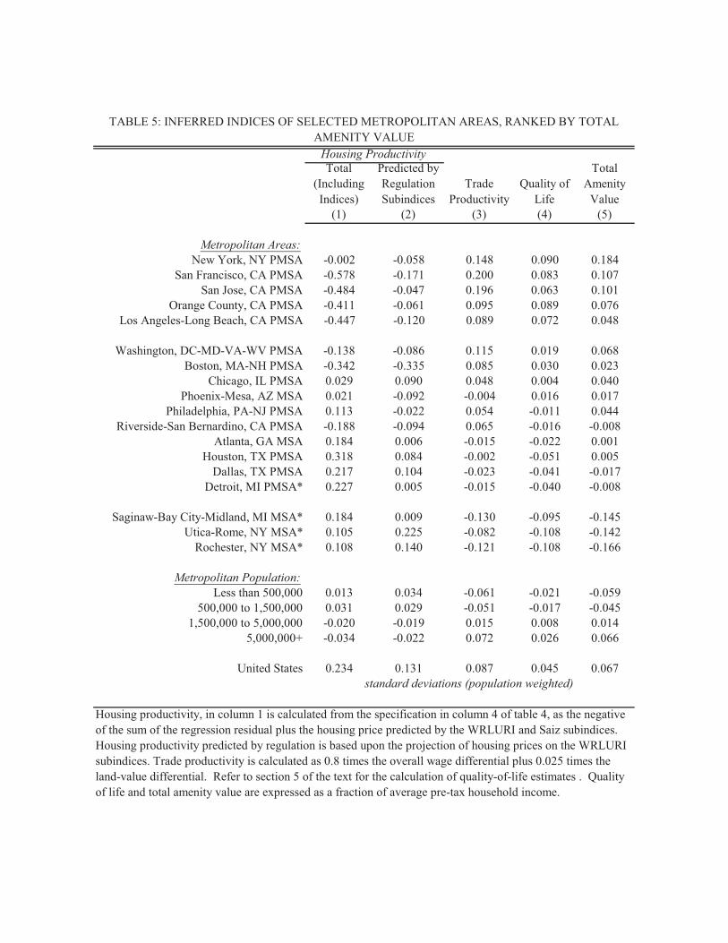
8��=��$#��=#��

'��#��#.)3��$��$.�#��

8��#�'��#$��+��)

K$��)��

8��1 ��);��$�

��

�� "�C7��-0"7'@�1 �� & ��& ��!� ��&�

��0B1'@�1 �� & �� &� ��F��0B1'@�1 ��&� �� !� ��

/��B�$�)0B1'@�1 �� ! ��&! ��1��9��*0B1'@�1 �� &! �� &

5��*��06B�@6�;1�5;'@�1 ��& ��&� �� ! ��&9��0@1�"E'@�1 �� & ��

B*��0=�'@�1 ��! ��!� ��& �� '*��,�@��01G@�1 �� !� ��

'*��#��*��0'1�"F'@�1 �� 3�+��#��9��#��0B1'@�1 ��&& ��!� �� &

1��0?1@�1 ��&� �� E�$��08>'@�1 ��& ��&� �� 6��08>'@�1 ��

6��0@='@�1H �� &

��C�9�)B��)�@�#��#0@=@�1H ��&� ��! �� ! ��

819�: (="�:33:6="6=B:�/��:�:B8:6@:83/'/�=81"13:1�031"J:6978/81�1@:"=87;1�<:

��

� ) ) 0<��3� �0"7@�1H �� &� ��& ��3��*��0"7@�1H ��& �� & ��

��*� ��0�� !

��0��0 ��0�� ! �� 0 ��0�� 0��0�� ! �� & ��

0��0��I ��

<��#�� &� ��

E�$��#$��+��)0��$ ��$��#�� *��$ ��.��0��*��+��*��$ ��*��#$��$��*�*�$��#��#.)�*�53�<3=�#��$.�#��E�$��#$��+��)��#��#.)��$��.��#$��*��2��*�$��*�53�<3=�$.�#��8��#��#$��+��)��$��#��&�� *��+��C��#��$�� *��#�+��$�#��3�� *��,��*��$��4$��)�� K$��)��#�� )+��$��,��#��+��,*�$��*��#��

8��#�'��#$��+��)

E�$��'��#$��+��)

E�$��'��#�'��#��#.)3��$��

8��'��#$��+��)

8��'��#$��+��)"�3��

��

��'��$�� &��

"$ .��/.��+�� 1#2$��#3��4$��# �� &

��

5��*��#6��)6�� & ��

"$ .��/.��+�� 1#2$��#3��4$��# �� !� ��

819�:�('3/6<B8=;=87="8316:19�:1"6E/<�="?�:B8/3�1BB/36="?8/@:83/'/�=81"'/'<�18=/"1"66:"�=87

6��#��;��.��

3�.$�� #��# ��0 ��$��# .) B@�10 ��# � ��*�� 8��#� �# *�$�� #$��+��) #�� $��# �� .�� 8�� #$��+��) �� $��# �� & �� *�$�� #$��+��) ��$� �� #� ��#$��+��)� 5��*��# #��) #�� $��# �� *� ��$�� #��) �� *� ��$�� +��0C��*��#.)��$��

E�$��'��#$��+��)@��$��(��

E�$��'��#$��+��) �� &� ��!��!� �� !�

"��$��B�� > > > >1��B�� > >

"$ .��/.��+�� 1#2$��#3��4$��# ��

819�:�(K<1�=87/��=�:1"6E/<�="?'3/6<B8=;=876��#��;��.��(K$��)��

3�.$�� #��# ��0 ��$��# .) B@�10 � ��*�� K$��) �� $��# �� .�� E�$�� #$��+��) ��#��# .) ��$�� $��# �� .�� "��$�� ( *��# �� #�� #�)�0 F$�) *$ �#��)0 �$�� $�*��0 �$�� 0 �#2��) �� 0��*�� #�,� 1�� $#� �� $��0 #��)0 �� ##��-�� .��* ��0 +�� 0 �# �� C��* � �� #��0 �� 0 �#*��*��*��#��9��*�� 1�.�$)��

8��E�$��'��#$��+��)E�$��'��#$��+��)

'��#��#.)3��$��

1+��#$��+��)L�$.��$��.��)

��C��#$��+��)

��C�$.��$��.��)

��#+��$�

E�$��

��

"�C7��-

6�+��

'��#$��+��)��

1+��#$��+��)L�$.��$��.��)

��C��#$��+��)

��C�$.��$��.��)

��#�+��$��#��

E�$��

#��

�

�

��

"�C7��-

6�+��

'��#$��+��)��

��$��29(8*��C��#$��+��)��C�$.��$��.��)�*�$��* �

��$��11(8*��C��#$��+��)��C�$.��$��.��)�*�$��+��

1+��#$��+��)L�$.��$��.��)

��C��#$��+��)

��C�$.��$��.��)

��#+��$�

E�$��

��

"�C7��-

6�+��

'��#$��+��)��

1+��#$��+��)L�$.��$��.��)

��C��#$��+��)

��C�$.��$��.��)

��#�+��$��#��

E�$��

#��

�

�

��

"�C7��-

6�+��

'��#$��+��)��

��$��21(8*��C��#$��+��)��C�$.��$��.��)�*�$��+��

��$��19(8*��C��#$��+��)��C�$.��$��.��)�*�$��* �

1�.�)

9�� *� J�,+��

11�.��

E��#

9��3�$��

"�C/��H"��*+��

B��#��

1�.$4$��4$�F��-��+��

;��$��

��$��6��HB��B��+��#HB��$ .$�

1$��

3��*�6$�*�

6�+��@��

3�+��#�

��-�B��)8� ��'*��,

"�C��-H

'��#0/3

/��#�

9��

��;��

/�-��#

��

��6��

@��

/��B�$�)

��F��

��

1��

'*��#��*��

B*��

5��*��

��1�� "�C7��-

��

��

��

��&

E�$

��

�'��=

#�,

:+��+��1 ��3��*��H

�)��$��H8��#�H

9$��H

�

/-��*� �B��)

��3��-J�,+��

@� �*��

:�'��

1-��H

@�1��

'��.$��*HJ��B��)

��5��*=#��

6��B��+��#

E�$��

��&

��

�� #�;��$�=#�,

@:83/'/'M�� @�� @��

�� @��

N ��@��

��(��O�� &!�� K$�#��(��G��O�� &�0:��)��$.O��&��

��$��1C(E�$��'��+��#;��$��

New

Yor

k-N

orth

ern

New

Jer

sey-

Long

Isla

nd, N

Y-N

J-C

T-PA

CM

SALo

s A

ngel

es-R

iver

side

-Ora

nge

Cou

nty,

CA

CM

SA

Chi

cago

-Gar

y-K

enos

ha, I

L-IN

-WI C

MSA

Hou

ston

-Gal

vest

on-B

razo

ria, T

X

Figu

re 2

: Lan

d Sa

les

in S

elec

ted

Met

ro A

reas

:+��+��

1 ��

3��*��H�)��$��H

1�.�)8��#�H

9$��H

9�� *�

/-��*� �B��)��3��-

11�.��

@� �*��

E��#

9��3�$��

1-��H

"�C/��H"��*+��

B��#��

1�.$4$��4$�

F��-��+��

;��$��

'��.$��*H

J��B��)��$��

��5��*

=#��

6��H

6��

B��

B��+��#H

B��$ .$� 6�+��

@��

3�+��#�

��-�B��)

8� ��

'*��,

"�C��-H

'��#0/3

/��#�

9��

��;��

/�-��#

��6��

@��

/��B�$�)

��F��

��

E�$��1��

'*��#��*��B*��

5��*��

��1��

"�C7��-

��

��

��

��

��

B�

��$��'��6��

1 ��)

J�,+��

:�'��

@�1��

1$��3��*�6$�*�

��

��

�� #�;��$�=#�,

@:83/'/'

M�� @��

�� @��

�� @��

N ��@��

��(��O��

B�6G'B(��#�*��O�� !��

B:�G'B�0��#��O�� 0��0��

:��)��$.O��

��#�*��G��O��

��$��31(B��$��'��+��#;��$��

B$�+�� $�� 10 :�� #�� 6��0"�B�+��$��39(8*��6� ��B�� B$�+�0 ��#�� G'B

1 ��:+��+��

:�'��

@�1��

J�,+��

/-��*� �B��)3��*��H

�)��$��H

B��#��3��-

8��#�H

9$��H

1-��H

9��3�$��9�� *� "��*+��

@� �*��

1�.$4$��4$�

F��-��+��

1�.�)

"�C/��H11�.��

E��#

'��.$��*HB��+��#HJ��B��)

8� ��

B��$ .$�

=#��

/��#�B��

��-�B��)1$��

3��*�6$�*�

��$��

��5��*

'��#0/3

6��

@��

6��H

6�+��

'*��,

@��

3�+��#�

��

�� 6��

��;��

9��"�C��-H

1��

E�$��

B*��

'*��#��*��

5��*��

"�C7��-

��

��

��

��

��

E�$

��

'��#$

��+��)

;��$��

��6��/��B�$�)/�-��#

��F��

��

��1��

��

��

�� 8��#�'��#$��+��)

@:83/'/'

M�� @��

�� @��

�� @��

N ��@��

8��#�'��#�9��E�$��'��#�<-�C

8��'��#��"��1+��(��O��

8��'��#$��+��)��%N"��1+��

8��'��#$��+��)��%M"��1+��

��(��O��&��&�

��4('��#$��+��)��*�8��#��.��#E�$��

1 ��

;��$��

E��# 11�.��

J�,+��

"�C/��H

9�� *�

1�.$4$��4$�

9��3�$��

"��*+��

��3��-

B��#��F��-��+��

/-��*� �B��)

@� �*��

1-��H

:�'�� @�1��

��

��F��

/�-��#

/��B�$�)

��6��

"�C��-H

9��

3�+��#�

��

6�+��

'��#0/3

@��

3��*�6$�*�

'*��,

1$��

��-�B��)

@��

��$��

8� ��/��#�

��;��

B��

6��6��H

B��$ .$�

��5��*

J��B��)=#��

B��+��#H

'��.$��*H

��1��

5��*��

"�C7��-

B*��

'*��#��*��

1��

E�$��

��

��

��

��

K$�

��)��

:+��+��1�.�)

3��*��H

8��#�H

�)��$��H

9$��H

��

��! ��& �� E�$��'��#$��+��)

@:83/'/'M�� @�� @�� @��N ��@��

��(��O��!!��!�

��$��5(K$��)��+��E�$��'��#$��+��)

Metropolitan Land Values and Housing Productivitygroups.haas.berkeley.edu/realestate/seminars/Papers...

Documents

Transcript of Metropolitan Land Values and Housing Productivitygroups.haas.berkeley.edu/realestate/seminars/Papers...