MetropolisMonteCarlosimulationoftheIsing Model -...
43
Metropolis Monte Carlo simulation of the Ising Model Krishna Shrinivas (CH10B026) Swaroop Ramaswamy (CH10B068) May 10, 2013 Modelling and Simulation of Particulate Processes (CH5012)
Transcript of MetropolisMonteCarlosimulationoftheIsing Model -...
Metropolis Monte Carlo simulation of the IsingModel
Krishna Shrinivas (CH10B026)Swaroop Ramaswamy (CH10B068)
May 10, 2013
Modelling and Simulation of Particulate Processes (CH5012)
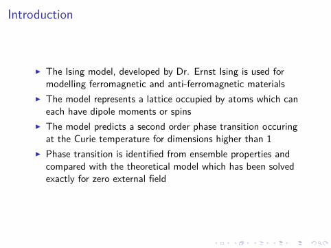
Introduction
I The Ising model, developed by Dr. Ernst Ising is used formodelling ferromagnetic and anti-ferromagnetic materials
I The model represents a lattice occupied by atoms which caneach have dipole moments or spins
I The model predicts a second order phase transition occuringat the Curie temperature for dimensions higher than 1
I Phase transition is identified from ensemble properties andcompared with the theoretical model which has been solvedexactly for zero external field

Ferromagnetism
I One of the fundamental properties of an electron is that it hasa dipole moment
I This dipole moment comes from the more fundamentalproperty of the electron that it has quantum mechanical spin
I The quantum mechanical nature of this spin causes theelectron to only be able to be in two states, with the magneticfield either pointing "up" or "down"
I When these tiny magnetic dipoles are aligned in the samedirection, their individual magnetic fields add together tocreate a measurable macroscopic field

Ferromagnetism
I Ferromagnetic materials are strongly ordered and have netmagnetization per site as −1/1 under temperatures T < Tc
I They are able to maintain spontaneous magnetization evenunder the absence of external fields
I At temperatures above Tc , the tendency to stay ordered isdisrupted due to competing effects from thermal motion
I The ferromagnetic substance behaves like a paramagneticsubstance at T > TC , showing no spontaneous magnetization

Ferromagnetism
I The reason for this strong alignment/bonding arises fromexchange interactions between electrons
I These exchange interactions are ≈1000 times more strongerthan dipole interactions, characteristic of paramagnetic anddiamagnetic substances
I In antiferromagnetic materials, these exchange interactionstend to favor the alignment of neighbouring atoms withopposite spins
I As far as the Ising Model goes, coupling parameter J > 0 forferromagnetic substances and J < 0 for antiferromagneticsubstances

Hamiltonian
I Each atom can adopt two states, corresponding tos = {−1, 1}, where s represents the spin and the spininteractions are dependent on the coupling parameter Jij
I The lattice model has periodic boundary conditions andextends infinitely
I This model is defined in the Canonical Ensemble(N,V ,T )and the Hamiltonian is defined as below
H = −Jij∑<i j>
sisj − h∑
isi
where,Jij= Coupling parameter between the adjacent atomsh = External Field Strengthsi ,j = Spin of particle

Partition Function
The Partition function corresponding to the Hamiltonian for theabove model is defined as:
Qpartition =∑
statese−βH
where β = 1kbT , kb → Boltzmann Constant

Ising 2-D Square ModelFor an isotropic case, where the coupling along the rows andcolumns are equal, the critical temperature has been found to be
kBTcJ =
2ln(1+
√2)≈ 2.269
The 2-D square model in the absence of an external field has beensolved (Lars Onsager, 1944) in the absence of an external field(h = 0)Internal Energy:
U =< H >=
∑states
He−βH
Qpartition
Isothermal Susceptibility:
χT = (dMdh )h =
1kBT (< M2
v > − < Mv >2)
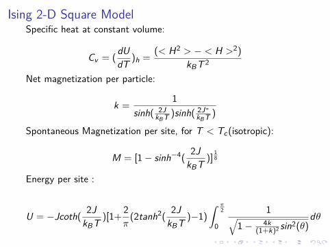
Ising 2-D Square ModelSpecific heat at constant volume:
Cv = (dUdT )h =
(< H2 > − < H >2)
kBT 2
Net magnetization per particle:
k =1
sinh( 2JkBT )sinh( 2J∗
kBT )
Spontaneous Magnetization per site, for T < Tc(isotropic):
M = [1− sinh−4(2J
kBT )]18
Energy per site :
U = −Jcoth( 2JkBT )[1+ 2
π(2tanh2(
2JkBT )−1)
ˆ π2
0
1√1− 4k
(1+k)2 sin2(θ)dθ

Applicability of Monte Carlo simulations
I The rationale behind Monte Carlo sampling techniques isinherently based on the sampling of time steps from anexponentially distributed function and making stochasticdecisions
I Since the Canonical ensemble arises from an exponentialdistribution of states, a similar rationale can be used tosample across the different states of the system untilequilibrium is reached

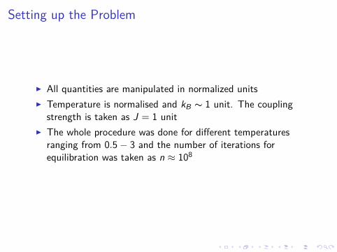
Setting up the Problem
I An optimal value of 900 atoms was chosen to model thissystem with periodic boundary conditions
I The lattice was represented by a 31× 31 random matrix, witheach element being randomly assigned with the values -1 or 1
It is chosen as a 31× 31 matrix so as to ensure that all the edgesare periodic in nature. The values at the first and last column, firstand last row are made the same
Setting up the Problem
I All quantities are manipulated in normalized unitsI Temperature is normalised and kB ∼ 1 unit. The coupling
strength is taken as J = 1 unitI The whole procedure was done for different temperatures
ranging from 0.5− 3 and the number of iterations forequilibration was taken as n ≈ 108

Initial Lattice Structure
Figure: Intial lattice, blue squares represent s = 1 and red squaresrepresent s = −1
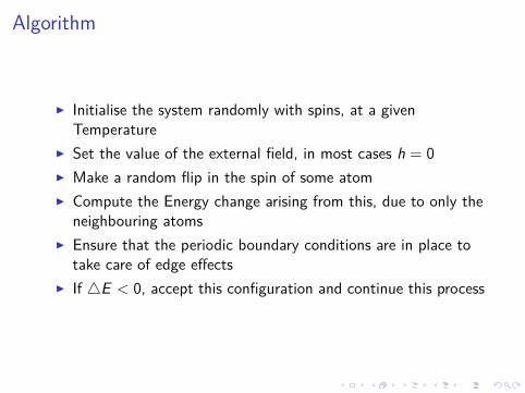
Algorithm
I Initialise the system randomly with spins, at a givenTemperature
I Set the value of the external field, in most cases h = 0I Make a random flip in the spin of some atomI Compute the Energy change arising from this, due to only the
neighbouring atomsI Ensure that the periodic boundary conditions are in place to
take care of edge effectsI If 4E < 0, accept this configuration and continue this process
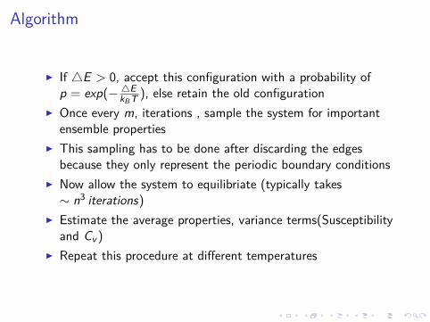
Algorithm
I If 4E > 0, accept this configuration with a probability ofp = exp(− 4E
kBT ), else retain the old configurationI Once every m, iterations , sample the system for important
ensemble propertiesI This sampling has to be done after discarding the edges
because they only represent the periodic boundary conditionsI Now allow the system to equilibriate (typically takes∼ n3 iterations)
I Estimate the average properties, variance terms(Susceptibilityand Cv )
I Repeat this procedure at different temperatures
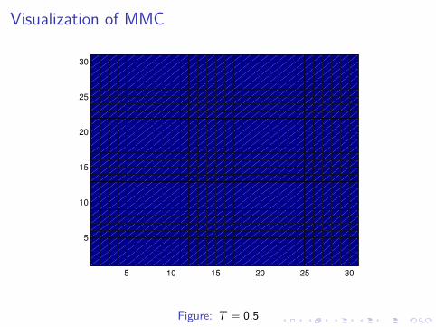
Visualization of MMC
5 10 15 20 25 30
5
10
15
20
25
30
Figure: T = 0.5
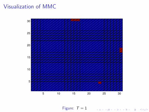
Visualization of MMC
5 10 15 20 25 30
5
10
15
20
25
30
Figure: T = 1
Visualization of MMC
5 10 15 20 25 30
5
10
15
20
25
30
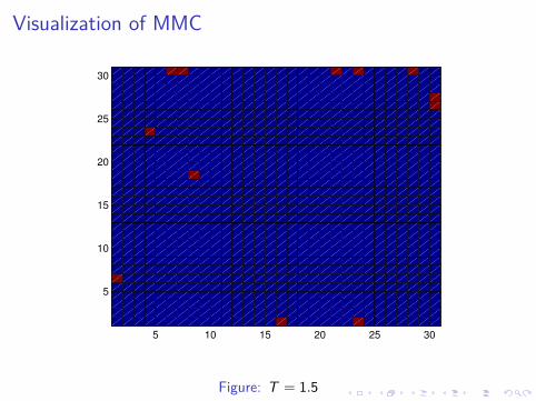
Figure: T = 1.5

Visualization of MMC
5 10 15 20 25 30
5
10
15
20
25
30
Figure: T = 2

Visualization of MMC
5 10 15 20 25 30
5
10
15
20
25
30
Figure: T = Tc ≈ 2.269

Visualization of MMC
5 10 15 20 25 30
5
10
15
20
25
30
Figure: T = 2.5

Visualization of MMC
5 10 15 20 25 30
5
10
15
20
25
30
Figure: T = 3

Visualization of MMC
5 10 15 20 25 30
5
10
15
20
25
30
Figure: T = 3.5
Visualization of MMC
5 10 15 20 25 30
5
10
15
20
25
30
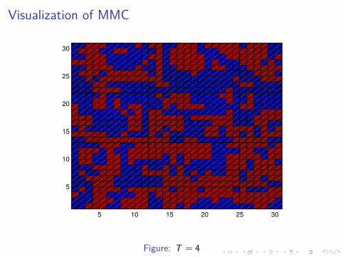
Figure: T = 4

Results
0.5 1 1.5 2 2.5 3−4
−3.5
−3
−2.5
−2
−1.5
−1
Temperature T
Energ
y p
er
ato
m
Energy per atom versus Temperature
Figure: Energy per site versus Temperature

Results
0.5 1 1.5 2 2.5 30
500
1000
1500
2000
2500
3000
3500
4000
4500
5000
Temperature T
Heat C
apacity
Heat Capacity versus Temperature
Figure: Heat Capacity versus Temperature

Results
0.5 1 1.5 2 2.5 30
0.1
0.2
0.3
0.4
0.5
0.6
0.7
0.8
0.9
1
Temperature T
Magnetization
Magnetization versus Temperature
Figure: Magnetization per site versus Temperature
Results
0.5 1 1.5 2 2.5 30
0.02
0.04
0.06
0.08
0.1
0.12
0.14
0.16
0.18
Temperature T
Magnetic S
usceptibili
ty p
er
ato
m
Magnetic Susceptibility versus Temperature
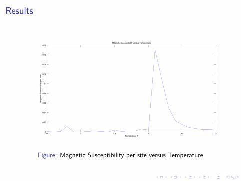
Figure: Magnetic Susceptibility per site versus Temperature

Ehrenfëst Classification of Phase Transitions
I For an nth order phase transition, at the transition point allthe nth order derivatives of the ensemble property diverge
I In the Ising model, both specific heat (Cv ) and magneticsusceptibility (χT ) have sharp discontinuites at the Curietemperature
I Since, Cv and χT are second order derivatives of ensembleproperties, this is classified as a second order phase transition

Physical understanding of the Phase Transition
I As the temperature increases, the tendency to stay orderedreduces because of thermal fluctuations
I The net magnetization, which is a function of net order in thesystem starts dropping
I Beyond the curie temperature Tc , there is no more tendencyto stay ordered, and due to complete disorderness, the netmagnetization per site drops to zero

Hysterisis
I The equilibriation is acheived with some value of h = l usingthe aforementioned algorithm
I Now h is slowly changed to h = −l in discrete stepsI During each of these steps, the previous equilibriated
configuration is given as input to the system to undergoequilibriation again
I Average and variance quantities are calculated and plotted

Results
−4 −3 −2 −1 0 1 2 3 4−1
−0.8
−0.6
−0.4
−0.2
0
0.2
0.4
0.6
0.8
1
External field strength
Magnetization p
er
site
Reverse/Decreasing Field Strength
Hysteresis increasing field strength
Figure: Hysteresis Loop

Critical Exponents
I Critical exponents describe the behaviour of physicalquantities near continuous phase transitions
I It is widely believed, but not proved formally, that theseexponents are independent of the physical properties of thesystem at consideration
I These only depend on the following propertiesI Dimension of interactionI Range of InteractionI Spin Dimension

Critical Exponents
I Near the phase transition temperature TC , we define thereduced Temperature τ = (T−Tc)/Tc
I It is stipulated that properties of the system, fi vary in apower law order, i.e., f ∝ τγ , asymptotically as τ → 0
I Some fluctuations are only observed in one phase, i.e. orderedor disordered
I The difference in the phases is determined by the orderparameter ψ, which is Magnetization for Ferromagneticmaterials

Critical Exponents
I Some important critical exponents are defined for CV ∝ τ−α,ψ ∝ (−τ)β and χT ∝ τ−γ
I These are estimated from the simulations performed throughPartial Least Squares Regression Technique(of the log values)
I
Analytical Simulation (MMC)α 0 0.013β 1/8 0.1288γ 7/4 1.81
Table: Comparison of Analytical and Simulation based CriticalExponents

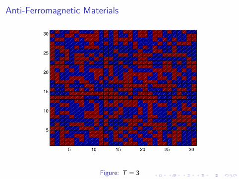
Anti-Ferromagnetic Materials
I For, anti-ferro magnetic materials, the coupling parameterJ < 0 between spins.
I This ensures that all the spins are always oppositely aligned atT < Tc,as this maximizes the energy(From the Hamiltonian)of the system.
I Since it is symmetric with all other respects(exceptMagnetization), all the variation in ensemble propertiesresemble those of the ferromagnetic system
I At temperatures beyond T > TC , the thermal fluctuationsstart to weigh in and the tendency to remain ordered isremoved
Anti-Ferromagnetic Materials
5 10 15 20 25 30
5
10
15
20
25
30
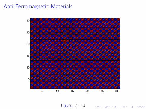
Figure: T = 1
Anti-Ferromagnetic Materials
5 10 15 20 25 30
5
10
15
20
25
30
Figure: T = 3

Anti-Ferromagnetic Materials
I Antiferromagnetic materials always prefer neighbouring atomsto have alternating spins. Hence presence of external fielddoes not impose any kind of magnetization on the material.This is observed from the simulations that the NetMagnetization Per Atom M, is invariant under external fields
I Since there is no external way to magnetize the system and astate having zero net magnetization is preferred, these kind ofmaterials do not show any cyclic properties or hysteresis loops.

Conclusions
I Phase transition is observed and signified by the change in theorder parameter(ψ)/net magentization(M) with increasingtemperature in the absence of any external field
I Phase transition is observed (ordered to disordered state) atthe curie Temperature of Tc ≈ 2.26, in agreement with theanalytical result.
I This phase transition is characterized as a second order phasetransition based on the divergence/discontinuity characteristicof the second derivative properties, for example MagneticSuscpetibility χT and Constant Volume Heat Capacity Cv .
Conclusions
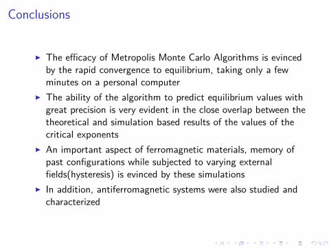
I The efficacy of Metropolis Monte Carlo Algorithms is evincedby the rapid convergence to equilibrium, taking only a fewminutes on a personal computer
I The ability of the algorithm to predict equilibrium values withgreat precision is very evident in the close overlap between thetheoretical and simulation based results of the values of thecritical exponents
I An important aspect of ferromagnetic materials, memory ofpast configurations while subjected to varying externalfields(hysteresis) is evinced by these simulations
I In addition, antiferromagnetic systems were also studied andcharacterized
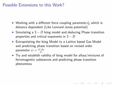
Possible Extensions to this Work?
I Working with a different force coupling parameterJij which isdistance dependent (Like Lennard-Jones potential)
I Simulating a 3−D Ising model and deducing Phase transitionproperties and critical exponents in 3− D
I Extrapolating the Ising Model to a Lattice based Gas Modeland predicting phase transition based on revised orderparameter ψ = ρ−ρc
ρc
I Try and establish validity of Ising model for alloys/mixtures offerromagnetic substances and predicting phase transitionphenomena

References
Onsager, Lars (1944), "Crystal statistics. I. A two-dimensionalmodel with an order-disorder transition", Phys. Rev. (2) 65(3–4): 117–149
Statistical Physics, 2nd edition, Landau&Lifshitz
Markov Processes, Gillespie, 4thedn
Class Notes!