Výsledky vyhodnocení splnění podmínek 2. veřejné soutěže ...
Upload
marina-coyCategory
view
228download
0
Metody odhadu budoucích klimatických podmínek II
Globální cirkulační modely, jejich výsledky a odhad budoucích klimatických podmínek pro střední
Evropu
Martin Dubrovský
www.ufa.cas.cz/dub/crop/crop.htm
Úvod
1.
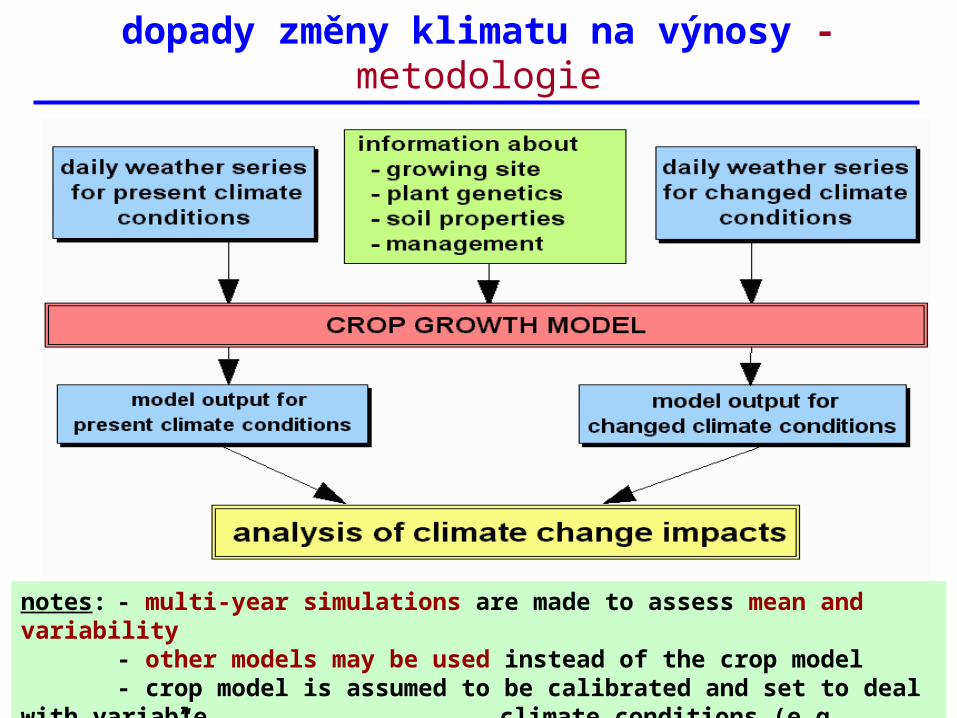
dopady změny klimatu na výnosy - metodologie
notes: - multi-year simulations are made to assess mean and variability- other models may be used instead of the crop model- crop model is assumed to be calibrated and set to deal with variable
climate conditions (e.g. “automatic” sowing day is used)

problém: Jak získat lokální meteorologické řady reprezentující budoucí klima?
- GCM?
+ v současnosti nejlepší dostupný nástroj k simulaci budoucího klimatu
+ množství GCM simulací současného i budoucího (i minulého) klimatu je volně dostupné na webu (např. databáze IPCC)
ale:? Jaká je kvalita výstupů z GCM ?
? Lze výstup z GCM použít jako vstup do impaktového modelu?
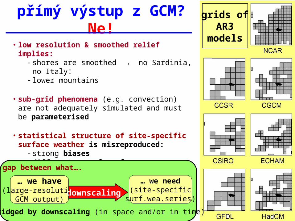
přímý výstup z GCM? Ne!
• low resolution & smoothed relief implies:- shores are smoothed → no Sardinia, no Italy!- lower mountains
• sub-grid phenomena (e.g. convection) are not adequately simulated and must be parameterised
• statistical structure of site-specific surface weather is misreproduced:
- strong biases - different annual cycle- different shape of PDFs (e.g. PREC)- different persistence (~ day-to-day variability)
grids ofAR3
models
… we have(large-resolution
GCM output)
… we need(site-specific
surf.wea.series)downscaling
• the gap between what….
is bridged by downscaling (in space and/or in time)
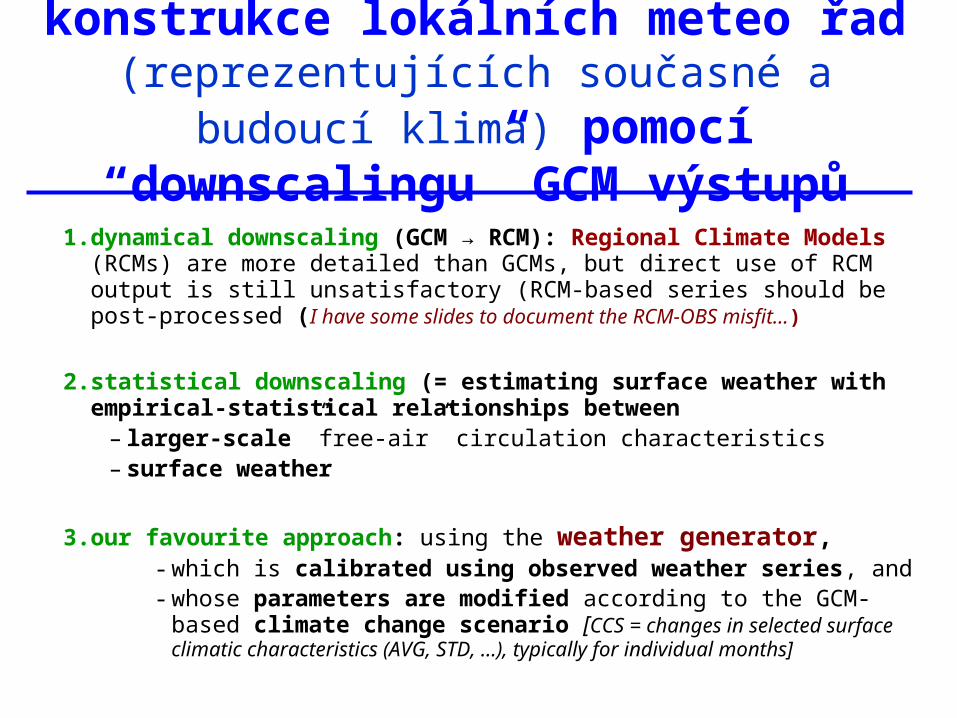
konstrukce lokálních meteo řad (reprezentujících současné a budoucí klima)
pomocí “downscalingu” GCM výstupů
1. dynamical downscaling (GCM → RCM): Regional Climate Models (RCMs) are more detailed than GCMs, but direct use of RCM output is still unsatisfactory (RCM-based series should be post-processed (I have some slides to document the RCM-OBS misfit…)
2. statistical downscaling (= estimating surface weather with empirical-statistical relationships between
– larger-scale ”free-air” circulation characteristics– surface weather
3. our favourite approach: using the weather generator,- which is calibrated using observed weather series, and- whose parameters are modified according to the GCM-based
climate change scenario [CCS = changes in selected surface climatic characteristics (AVG, STD, …), typically for individual months]
stochastickýmeteo generátor
+ scénáře změny klimatu
2 + 3
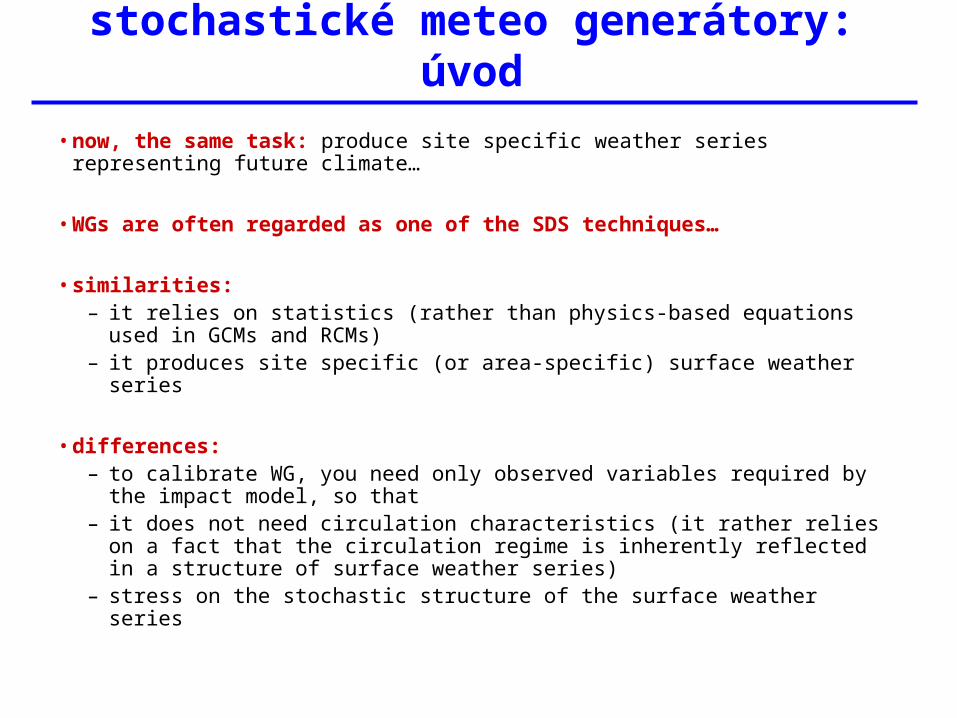
stochastické meteo generátory: úvod
• now, the same task: produce site specific weather series representing future climate…
• WGs are often regarded as one of the SDS techniques…
• similarities:– it relies on statistics (rather than physics-based equations used in
GCMs and RCMs)– it produces site specific (or area-specific) surface weather series
• differences:– to calibrate WG, you need only observed variables required by the
impact model, so that– it does not need circulation characteristics (it rather relies on a fact that
the circulation regime is inherently reflected in a structure of surface weather series)
– stress on the stochastic structure of the surface weather series
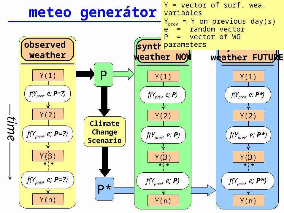
meteo generátor
observed weather
:::
time
Y(3)
Y(n)
f(Yprev, e; P=?)
f(Yprev, e; P=?)
f(Yprev, e; P=?)
Y(2)
Y(1)
ClimateChange
Scenario
synthetic weather NOW
:::Y(3)
Y(n)
f(Yprev, e; P)
f(Yprev, e; P)
f(Yprev, e; P)
Y(2)
Y(1)
synthetic weather FUTURE
:::Y(3)
Y(n)
f(Yprev, e; P*)
f(Yprev, e; P*)
f(Yprev, e; P*)
Y(2)
Y(1)P
P*
Y = vector of surf. wea. variablesYprev = Y on previous day(s)e = random vectorP = vector of WG parameters
použití sWGpři konstrukci meteo řad
reprezentujících budoucí klima
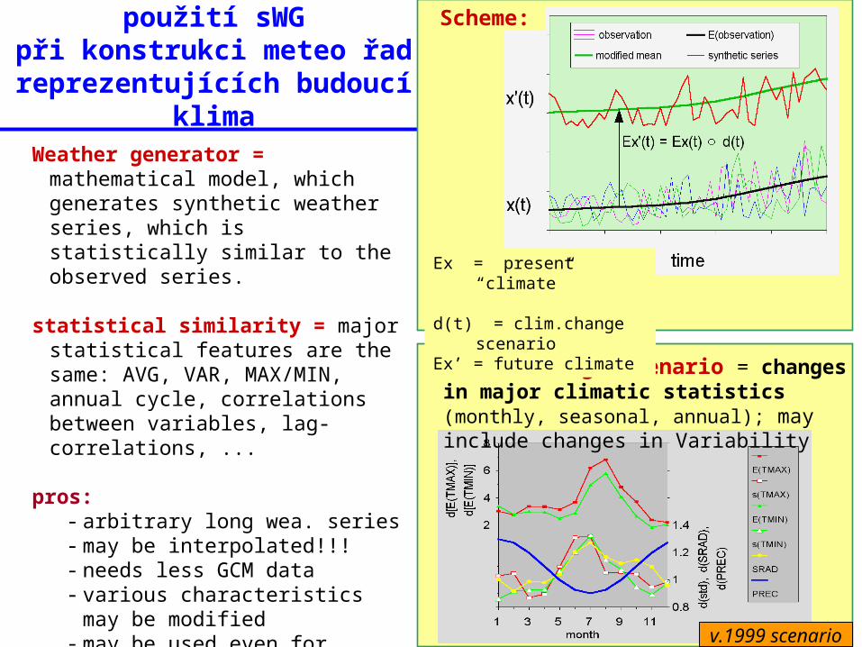
Weather generator = mathematical model, which generates synthetic weather series, which is statistically similar to the observed series.
statistical similarity = major statistical features are the same: AVG, VAR, MAX/MIN, annual cycle, correlations between variables, lag-correlations, ...
pros:- arbitrary long wea. series- may be interpolated!!!- needs less GCM data- various characteristics may be
modified- may be used even for climates not
simulated by GCM (using pattern scaling method)
con: no WG model is perfect…
Climate change scenario = changes in major climatic statistics (monthly, seasonal, annual); may include changes in Variability
Ex = present “climate”
d(t) = clim.change scenarioEx’ = future climate
Scheme:
v.1999 scenario
stochastické meteo generátory
part 2
stoch. meteo generátory: jak fungujípříklad: M&Rfi
(parametrický meteo generátor)
• M&Rfi weather generator (~ Richardson’s WGEN)– generates daily time series– 4 surface weather characteristics (though it can do much
more…), which are mostly required as an input to the crop growth models (including DSSAT crop models):
• PREC, TMAX, TMIN, SRAD
• each term is generated in three steps:1. generation of precipitation occurrence ~ 1st order Markov chain
2. (if the day is wet) generation of precipitation amount: PREC ~ Gamma dist.
3. generation of (SRAD, TMAX, TMIN) ~ AR(1) model
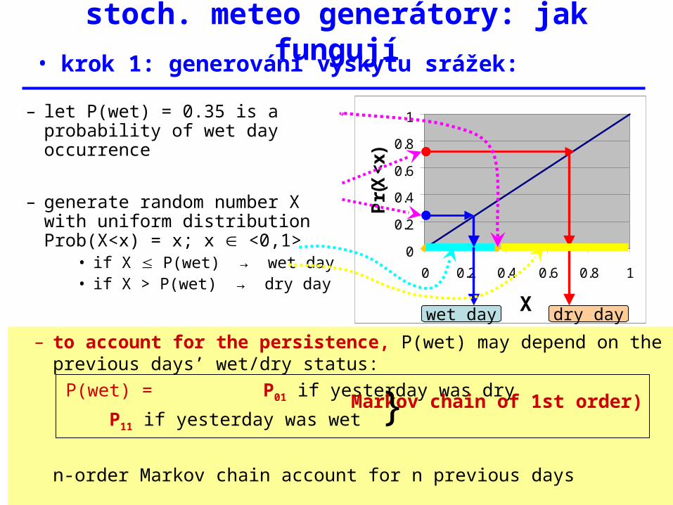
stoch. meteo generátory: jak fungují• krok 1: generování výskytu srážek:
0
0.2
0.4
0.6
0.8
1
0 0.2 0.4 0.6 0.8 1
X
Pr(
X<
x)
– let P(wet) = 0.35 is a probability of wet day occurrence
– generate random number X with uniform distribution Prob(X<x) = x; x <0,1>
• if X P(wet) → wet day• if X > P(wet) → dry day
wet day dry day
– to account for the persistence, P(wet) may depend on the previous days’ wet/dry status:
P(wet) = P01 if yesterday was dry
P11 if yesterday was wet
n-order Markov chain account for n previous days
Markov chain of 1st order)}
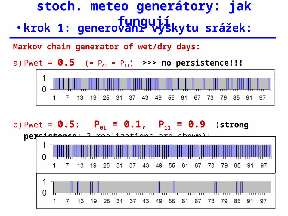
stoch. meteo generátory: jak fungují• krok 1: generování výskytu srážek:
Markov chain generator of wet/dry days:
a) Pwet = 0.5 (= P01 = P11) >>> no persistence!!!
b) Pwet = 0.5; P01 = 0.1, P11 = 0.9 (strong persistence; 2
realizations are shown):
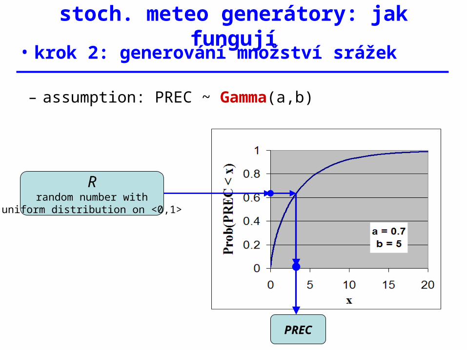
stoch. meteo generátory: jak fungují• krok 2: generování množství srážek
– assumption: PREC ~ Gamma(a,b)
PREC
Rrandom number with
uniform distribution on <0,1>
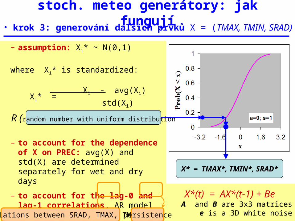
stoch. meteo generátory: jak fungují• krok 3: generování dalších prvků X = (TMAX, TMIN, SRAD)
– assumption: Xi* ~ N(0,1)
where Xi* is standardized:
Xi - avg(Xi) Xi* = std(Xi)
– to account for the dependence of X on PREC: avg(X) and std(X) are determined separately for wet and dry days
– to account for the lag-0 and lag-1 correlations, AR model is used:
X* = TMAX*, TMIN*, SRAD*
R (random number with uniform distribution
X*(t) = AX*(t-1) + BeA and B are 3x3 matrices
e is a 3D white noisecorelations between SRAD, TMAX, TMINpersistence
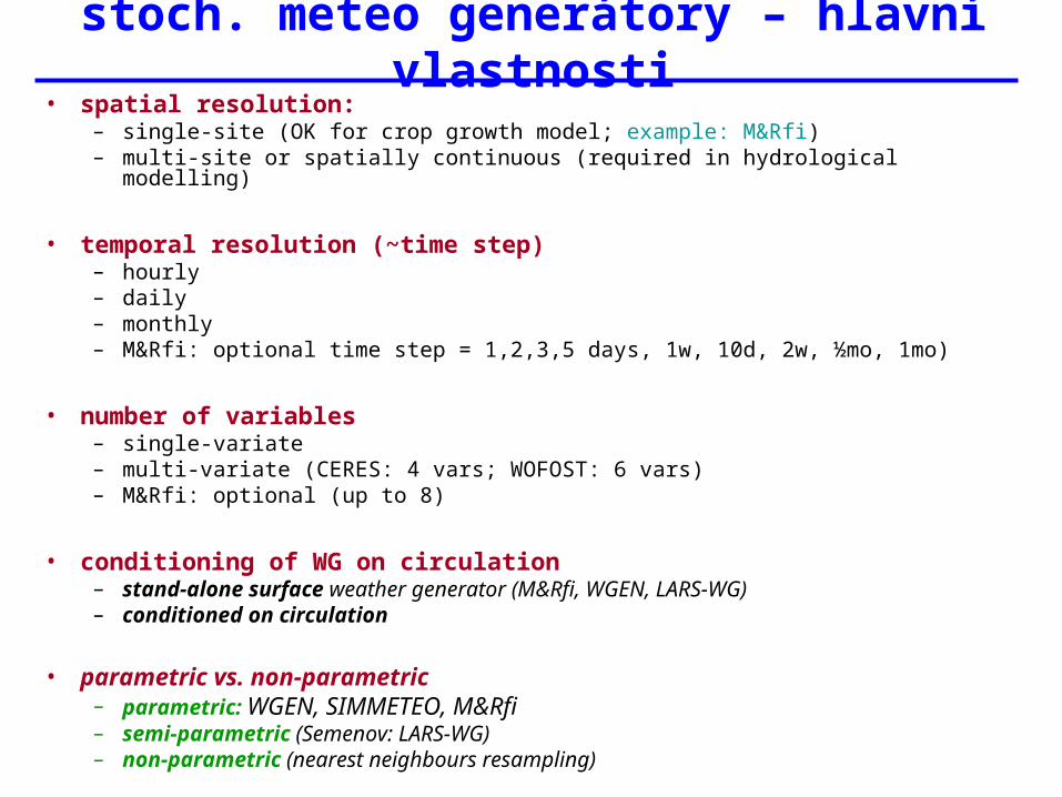
stoch. meteo generátory – hlavní vlastnosti• spatial resolution:
– single-site (OK for crop growth model; example: M&Rfi)– multi-site or spatially continuous (required in hydrological modelling)
• temporal resolution (~time step)– hourly– daily– monthly– M&Rfi: optional time step = 1,2,3,5 days, 1w, 10d, 2w, ½mo, 1mo)
• number of variables– single-variate– multi-variate (CERES: 4 vars; WOFOST: 6 vars)– M&Rfi: optional (up to 8)
• conditioning of WG on circulation– stand-alone surface weather generator (M&Rfi, WGEN, LARS-WG)– conditioned on circulation
• parametric vs. non-parametric– parametric: WGEN, SIMMETEO, M&Rfi– semi-parametric (Semenov: LARS-WG)– non-parametric (nearest neighbours resampling)
parametrické meteo generátory
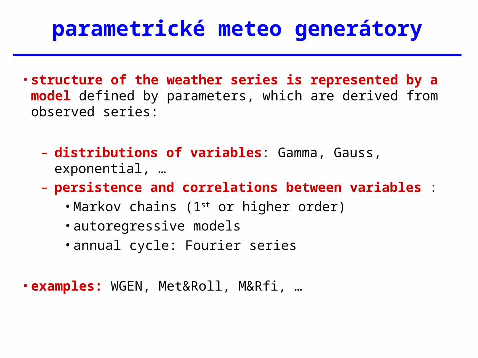
• structure of the weather series is represented by a model defined by parameters, which are derived from observed series:
– distributions of variables: Gamma, Gauss, exponential, …– persistence and correlations between variables :
• Markov chains (1st or higher order)• autoregressive models• annual cycle: Fourier series
• examples: WGEN, Met&Roll, M&Rfi, …
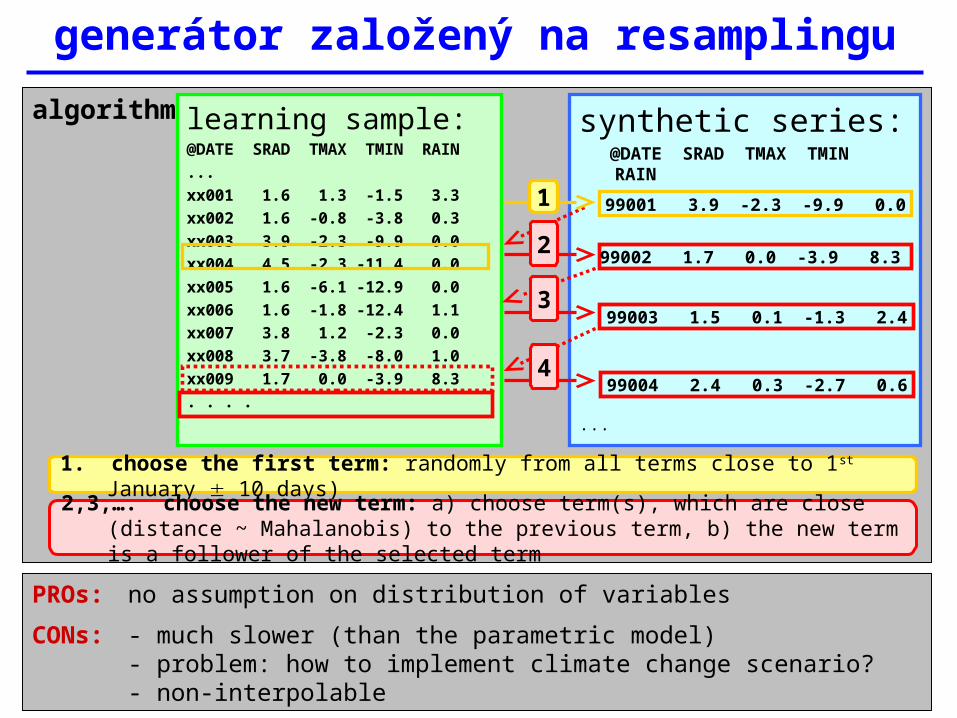
algorithm:
generátor založený na resamplingu
learning sample:@DATE SRAD TMAX TMIN
RAIN...xx001 1.6 1.3 -1.5 3.3xx002 1.6 -0.8 -3.8 0.3xx003 3.9 -2.3 -9.9 0.0xx004 4.5 -2.3 -11.4 0.0xx005 1.6 -6.1 -12.9 0.0xx006 1.6 -1.8 -12.4 1.1 xx007 3.8 1.2 -2.3 0.0xx008 3.7 -3.8 -8.0 1.0xx009 1.7 0.0 -3.9 8.3 . . . .
synthetic series: @DATE SRAD TMAX TMIN
RAIN
...
99002 1.7 0.0 -3.9 8.3
99003 1.5 0.1 -1.3 2.4
99004 2.4 0.3 -2.7 0.6
99001 3.9 -2.3 -9.9 0.01
1. choose the first term: randomly from all terms close to 1st January 10 days)
2
3
4
2,3,…. choose the new term: a) choose term(s), which are close (distance ~ Mahalanobis) to the previous term, b) the new term is a follower of the selected term
PROs: no assumption on distribution of variables
CONs: - much slower (than the parametric model)- problem: how to implement climate change scenario?- non-interpolable
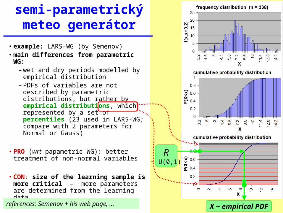
• example: LARS-WG (by Semenov)• main differences from parametric WG:
– wet and dry periods modelled by empirical distribution
– PDFs of variables are not described by parametric distributions, but rather by empirical distributions, which represented by a set of percentiles (23 used in LARS-WG; compare with 2 parameters for Normal or Gauss)
• PRO (wrt papametric WG): better treatment of non-normal variables
• CON: size of the learning sample is more critical ← more parameters are determined from the learning data
semi-parametrický meteo generátor
X ~ empirical PDF
R~ U(0,1)
references: Semenov + his web page, …
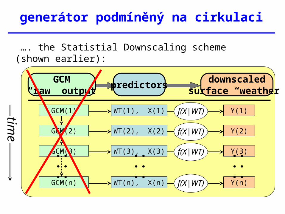
generátor podmíněný na cirkulaci
WT(1), X(1)
WT(2), X(2)
WT(3), X(3)
WT(n), X(n)
Y(1)
Y(2)
Y(3)
Y(n)
downscaledsurface “weather”
GCM(1)
GCM(2)
GCM(3)
GCM(n)
:::
:::
:::
f(X|WT)
f(X|WT)
f(X|WT)
f(X|WT)time
GCM“raw” output
predictors
…. the Statistial Downscaling scheme (shown earlier):
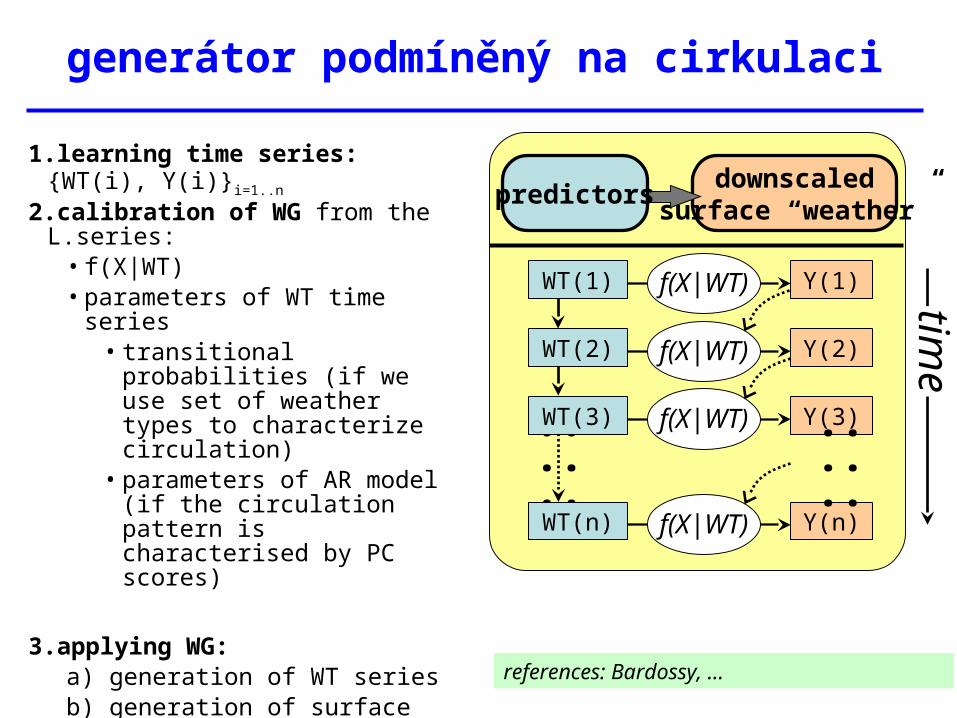
generátor podmíněný na cirkulaci
Y(1)
Y(2)
Y(3)
Y(n)
downscaledsurface “weather”
:::
:::
f(X|WT)
f(X|WT)
f(X|WT)
f(X|WT) time
predictors
1.learning time series: {WT(i), Y(i)}i=1..n
2.calibration of WG from the L.series:• f(X|WT)• parameters of WT time series
• transitional probabilities (if we use set of weather types to characterize circulation)
• parameters of AR model (if the circulation pattern is characterised by PC scores)
3.applying WG:a) generation of WT seriesb) generation of surface wea. series
PRO: circulation is explicitely involvedCON: we need future GCM simulation to
calibrate the WG’s circulation component > limited possibilities for uncertainty analysis
WT(1)
WT(2)
WT(3)
WT(n)
references: Bardossy, …
meteo generátor M&Rfi
… volně k dispozici na webu:www.ufa.cas.cz/dub/wg/marfi/marfi.htm
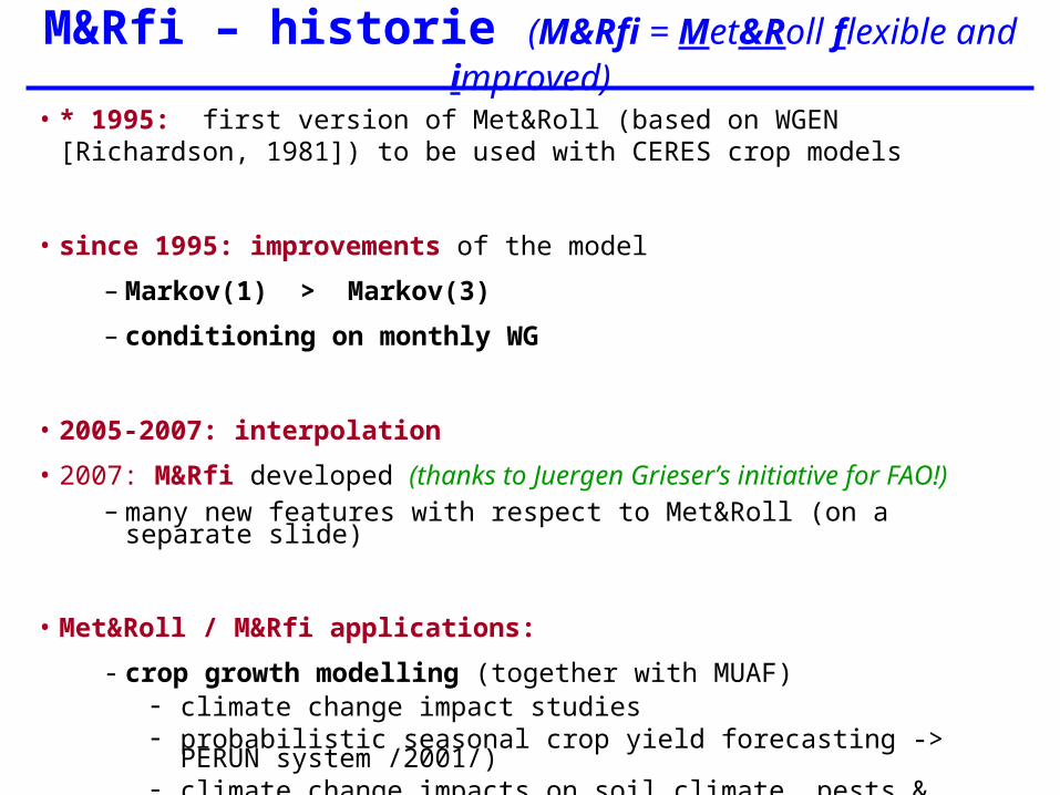
M&Rfi – historie (M&Rfi = Met&Roll flexible and improved)
• * 1995: first version of Met&Roll (based on WGEN [Richardson, 1981]) to be used with CERES crop models
• since 1995: improvements of the model
– Markov(1) > Markov(3)
– conditioning on monthly WG
• 2005-2007: interpolation
• 2007: M&Rfi developed (thanks to Juergen Grieser’s initiative for FAO!)– many new features with respect to Met&Roll (on a separate slide)
• Met&Roll / M&Rfi applications:
- crop growth modelling (together with MUAF)- climate change impact studies- probabilistic seasonal crop yield forecasting -> PERUN system /2001/)- climate change impacts on soil climate, pests & diseases, …
- hydrological modelling
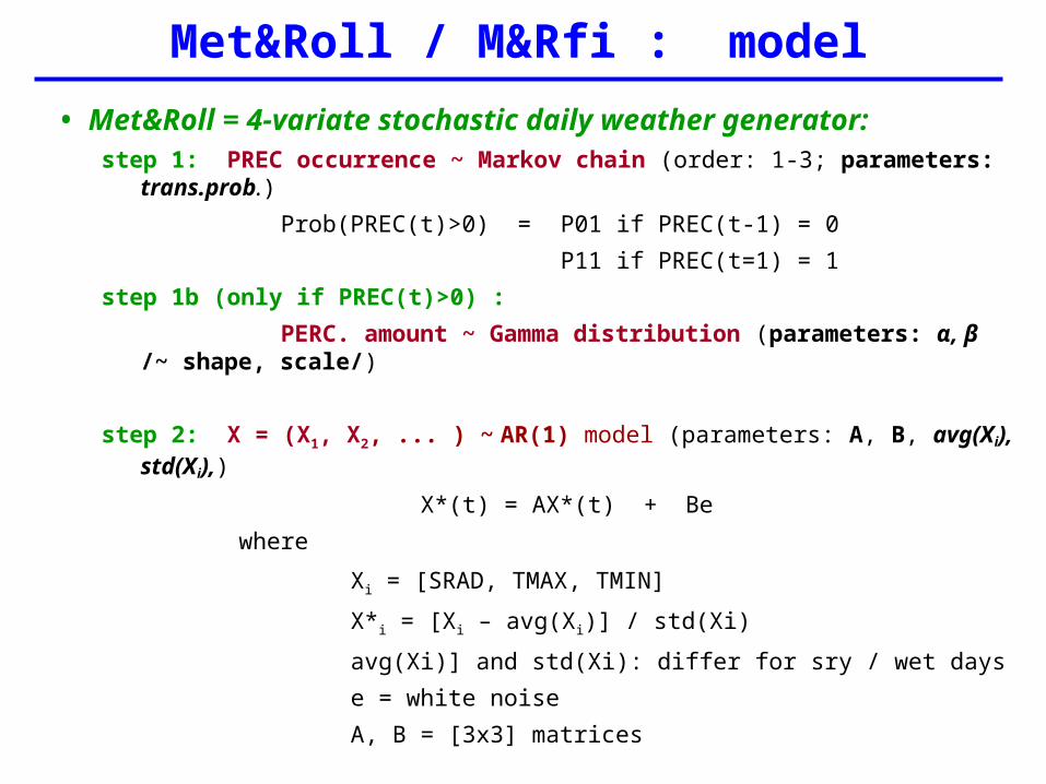
• Met&Roll = 4-variate stochastic daily weather generator:step 1: PREC occurrence ~ Markov chain (order: 1-3; parameters: trans.prob.)
Prob(PREC(t)>0) = P01 if PREC(t-1) = 0
P11 if PREC(t=1) = 1
step 1b (only if PREC(t)>0) :
PERC. amount ~ Gamma distribution (parameters: α, β /~ shape, scale/)
step 2: X = (X1, X2, ... ) ~ AR(1) model (parameters: A, B, avg(Xi), std(Xi),)
X*(t) = AX*(t) + Be
where
Xi = [SRAD, TMAX, TMIN]
X*i = [Xi – avg(Xi)] / std(Xi)
avg(Xi)] and std(Xi): differ for sry / wet days
e = white noise
A, B = [3x3] matrices
- all parameters are assumed to vary during the year
- daily WG is linked to AR(1)-based monthly WG (to improve low-frequency variability)
Met&Roll / M&Rfi : model
M&Rfi – hlavní vlastnosti
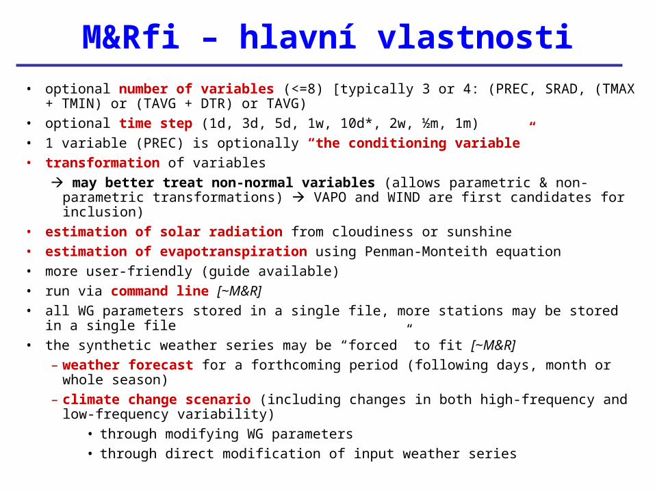
• optional number of variables (<=8) [typically 3 or 4: (PREC, SRAD, (TMAX + TMIN) or (TAVG + DTR) or TAVG)
• optional time step (1d, 3d, 5d, 1w, 10d*, 2w, ½m, 1m)
• 1 variable (PREC) is optionally “the conditioning variable”
• transformation of variables
may better treat non-normal variables (allows parametric & non-parametric transformations) VAPO and WIND are first candidates for inclusion)
• estimation of solar radiation from cloudiness or sunshine
• estimation of evapotranspiration using Penman-Monteith equation
• more user-friendly (guide available)
• run via command line [~M&R]
• all WG parameters stored in a single file, more stations may be stored in a single file
• the synthetic weather series may be “forced” to fit [~M&R]
– weather forecast for a forthcoming period (following days, month or whole season)
– climate change scenario (including changes in both high-frequency and low-frequency variability)
• through modifying WG parameters
• through direct modification of input weather series
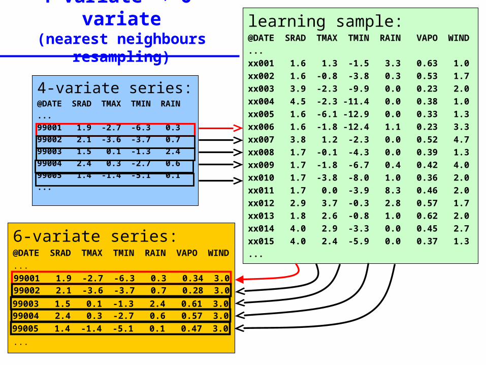
4-variate 6-variate(nearest neighbours resampling)
4-variate series:@DATE SRAD TMAX TMIN RAIN
...
99001 1.9 -2.7 -6.3 0.3
99002 2.1 -3.6 -3.7 0.7
99003 1.5 0.1 -1.3 2.4
99004 2.4 0.3 -2.7 0.6
99005 1.4 -1.4 -5.1 0.1
...
learning sample:@DATE SRAD TMAX TMIN RAIN VAPO
WIND...xx001 1.6 1.3 -1.5 3.3 0.63 1.0xx002 1.6 -0.8 -3.8 0.3 0.53 1.7xx003 3.9 -2.3 -9.9 0.0 0.23 2.0xx004 4.5 -2.3 -11.4 0.0 0.38 1.0xx005 1.6 -6.1 -12.9 0.0 0.33 1.3xx006 1.6 -1.8 -12.4 1.1 0.23 3.3xx007 3.8 1.2 -2.3 0.0 0.52 4.7xx008 1.7 -0.1 -4.3 0.0 0.39 1.3xx009 1.7 -1.8 -6.7 0.4 0.42 4.0xx010 1.7 -3.8 -8.0 1.0 0.36 2.0xx011 1.7 0.0 -3.9 8.3 0.46 2.0xx012 2.9 3.7 -0.3 2.8 0.57 1.7xx013 1.8 2.6 -0.8 1.0 0.62 2.0xx014 4.0 2.9 -3.3 0.0 0.45 2.7xx015 4.0 2.4 -5.9 0.0 0.37 1.3...
6-variate series:@DATE SRAD TMAX TMIN RAIN VAPO
WIND...
...
99001 1.9 -2.7 -6.3 0.3 0.34 3.099002 2.1 -3.6 -3.7 0.7 0.28 3.0
99003 1.5 0.1 -1.3 2.4 0.61 3.099004 2.4 0.3 -2.7 0.6 0.57 3.099005 1.4 -1.4 -5.1 0.1 0.47 3.0
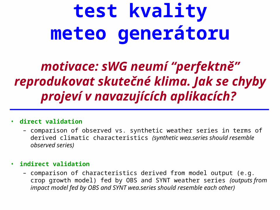
test kvalitymeteo generátoru
motivace: sWG neumí “perfektně” reprodukovat skutečné klima. Jak se chyby
projeví v navazujících aplikacích?
• direct validation
– comparison of observed vs. synthetic weather series in terms of derived climatic characteristics (synthetic wea.series should resemble observed series)
• indirect validation
– comparison of characteristics derived from model output (e.g. crop growth model) fed by OBS and SYNT weather series (outputs from impact model fed by OBS and SYNT wea.series should resemble each other)
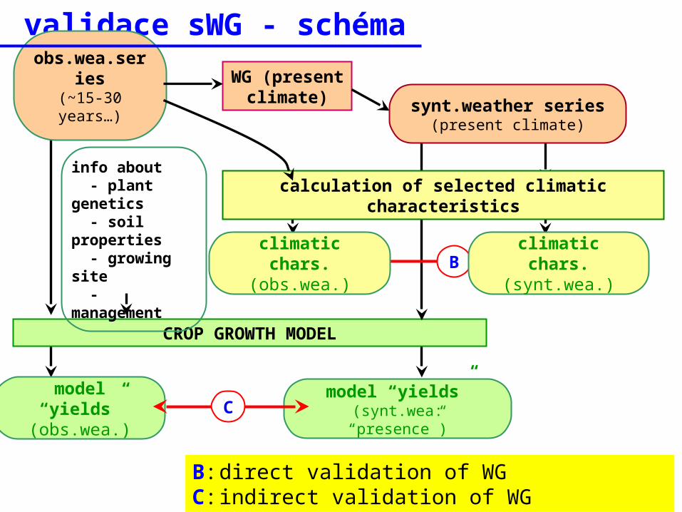
validace sWG - schéma
obs.wea.series(~15-30 years…)
model “yields”(obs.wea.)
CROP GROWTH MODEL
WG (present climate)
model “yields”(synt.wea: “presence”)
synt.weather series (present climate)
B
C
B: direct validation of WG C: indirect validation of WG
info about - plant genetics - soil properties - growing site - management
calculation of selected climatic characteristics
climatic chars.(obs.wea.)
climatic chars.(synt.wea.)
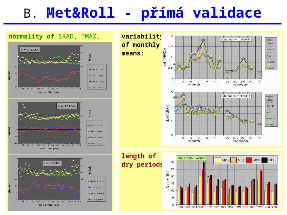
length ofdry periods:
variabilityof monthlymeans:
normality of SRAD, TMAX, TMIN:
B. Met&Roll - přímá validace
C. Met&Roll – nepřímá validace
Motivation:
How the WG imperfections (to fit the structure of real-
world weather series) affect output from impact models
fed by synthetic series?
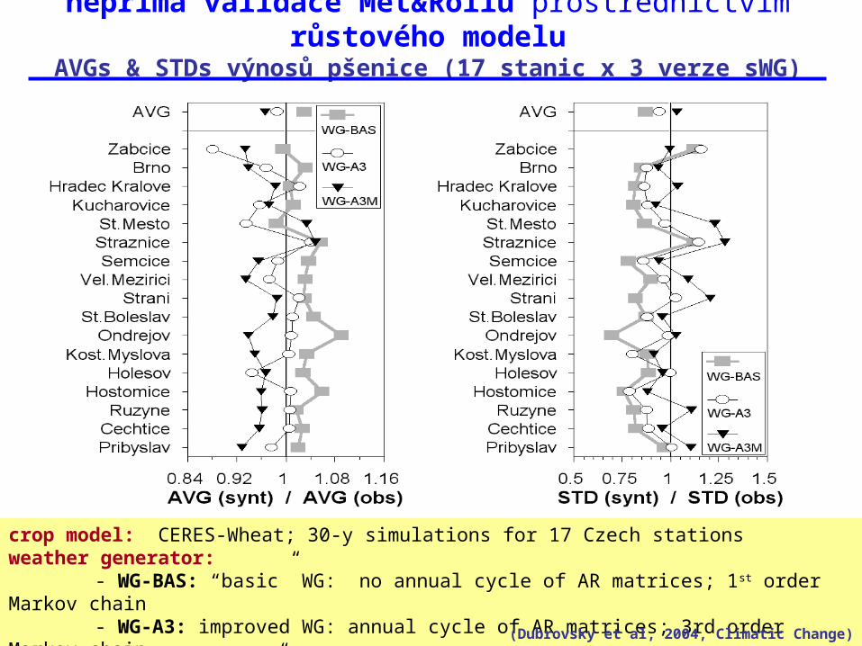
nepřímá validace Met&Rollu prostřednictvím růstového modeluAVGs & STDs výnosů pšenice (17 stanic x 3 verze sWG)
crop model: CERES-Wheat; 30-y simulations for 17 Czech stationsweather generator:
- WG-BAS: “basic” WG: no annual cycle of AR matrices; 1st order Markov chain- WG-A3: improved WG: annual cycle of AR matrices; 3rd order Markov chain- WG-A3M: “best” WG: WG-A3 + conditioned on monthly WG (Dubrovsky et al, 2004, Climatic Change)
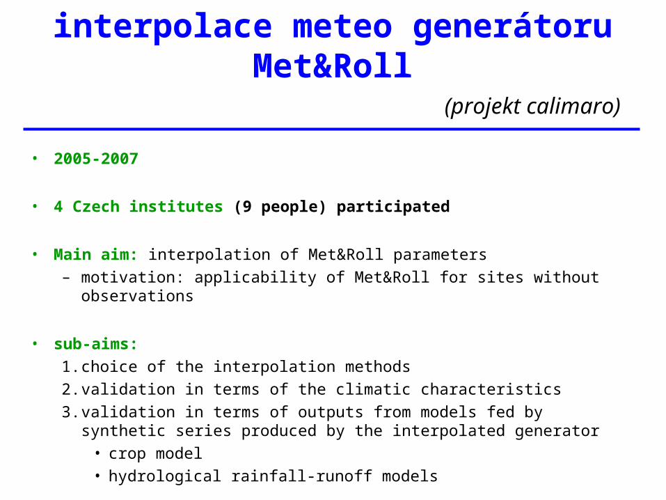
interpolace meteo generátoruMet&Roll
(projekt calimaro)
• 2005-2007
• 4 Czech institutes (9 people) participated
• Main aim: interpolation of Met&Roll parameters
– motivation: applicability of Met&Roll for sites without observations
• sub-aims:
1. choice of the interpolation methods
2. validation in terms of the climatic characteristics
3. validation in terms of outputs from models fed by synthetic series produced by the interpolated generator
• crop model
• hydrological rainfall-runoff models
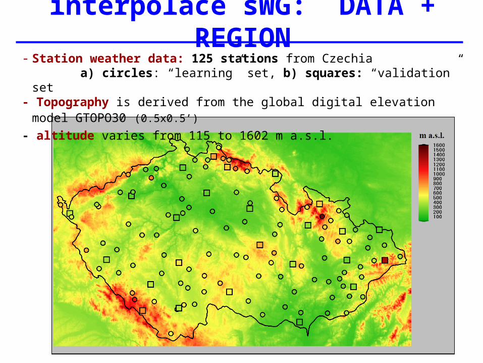
interpolace sWG: DATA + REGION- Station weather data: 125 stations from Czechia
a) circles: “learning” set, b) squares: “validation” set- Topography is derived from the global digital elevation model GTOPO30 (0.5x0.5’)
- altitude varies from 115 to 1602 m a.s.l.
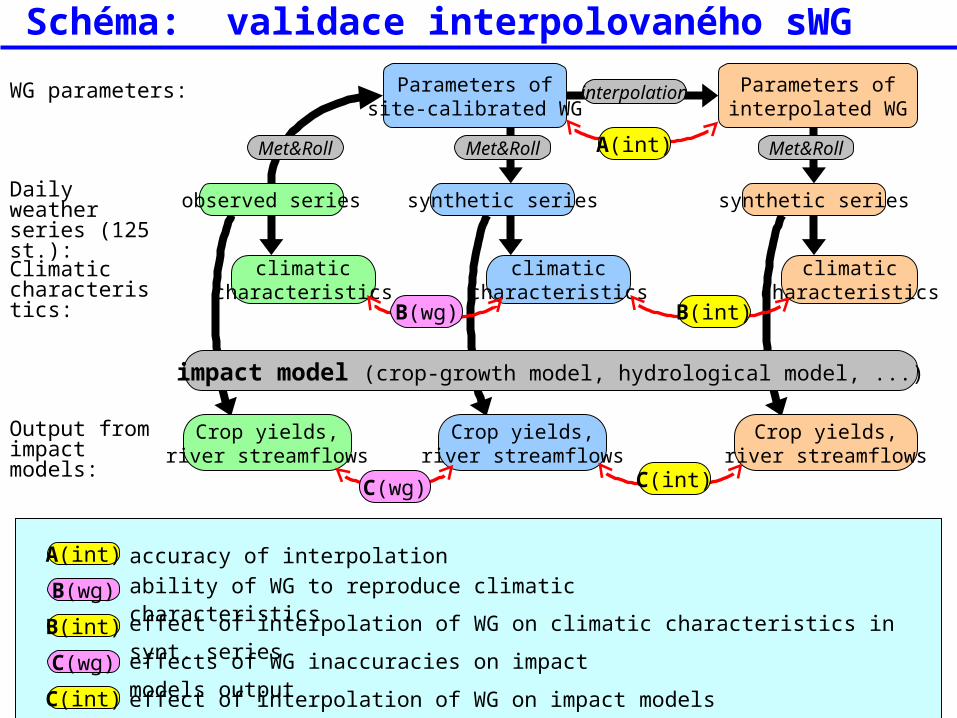
Schéma: validace interpolovaného sWG
climaticcharacteristics
climaticcharacteristics
climaticcharacteristics
Crop yields,river streamflows
Crop yields,river streamflows
Crop yields,river streamflows
impact model (crop-growth model, hydrological model, ...)
Parameters ofinterpolated WG
interpolation
Met&Roll
Parameters ofsite-calibrated WG
synthetic series
Met&Roll
synthetic series
Met&RollA(int)
accuracy of interpolationA(int)
C(wg)
effects of WG inaccuracies on impact models outputC(wg)
C(int)
effect of interpolation of WG on impact models outputC(int)
B(wg)
ability of WG to reproduce climatic characteristicsB(wg)
WG parameters:
Daily weather series (125 st.):
Climaticcharacteristics:
Output fromimpact models:
B(int)
effect of interpolation of WG on climatic characteristics in synt. seriesB(int)
observed series
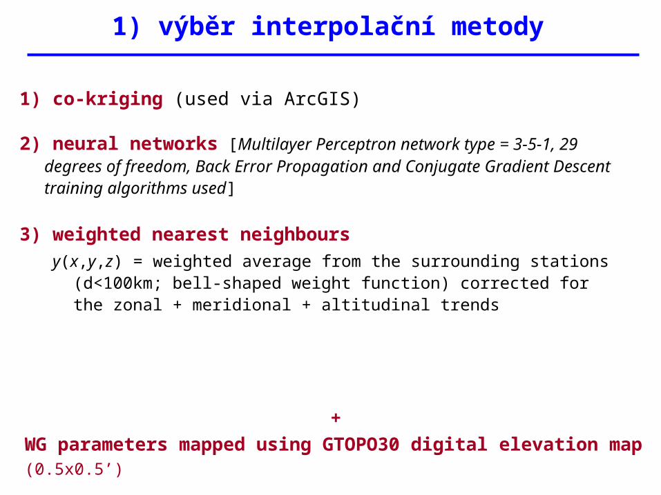
1) výběr interpolační metody
1) co-kriging (used via ArcGIS)
2) neural networks [Multilayer Perceptron network type = 3-5-1, 29 degrees of freedom, Back Error Propagation and Conjugate Gradient Descent training algorithms used]
3) weighted nearest neighbours
y(x,y,z) = weighted average from the surrounding stations (d<100km; bell-shaped weight function) corrected for the zonal + meridional + altitudinal trends
+
WG parameters mapped using GTOPO30 digital elevation map (0.5x0.5’)
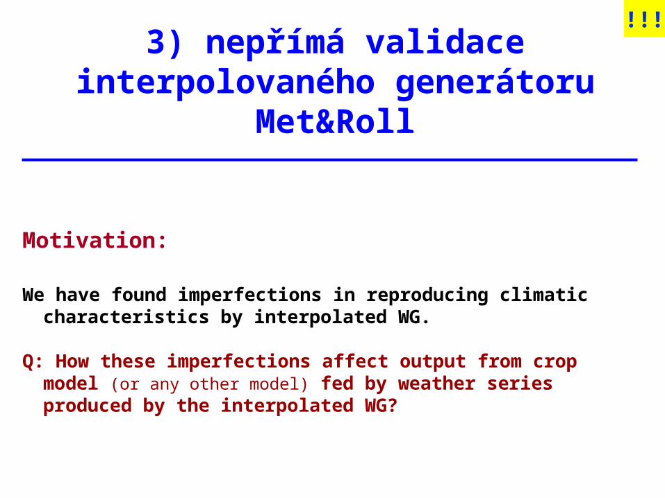
3) nepřímá validaceinterpolovaného generátoru Met&Roll
Motivation:
We have found imperfections in reproducing climatic characteristics by interpolated WG.
Q: How these imperfections affect output from crop model (or any other model) fed by weather series produced by the interpolated WG?
!!!
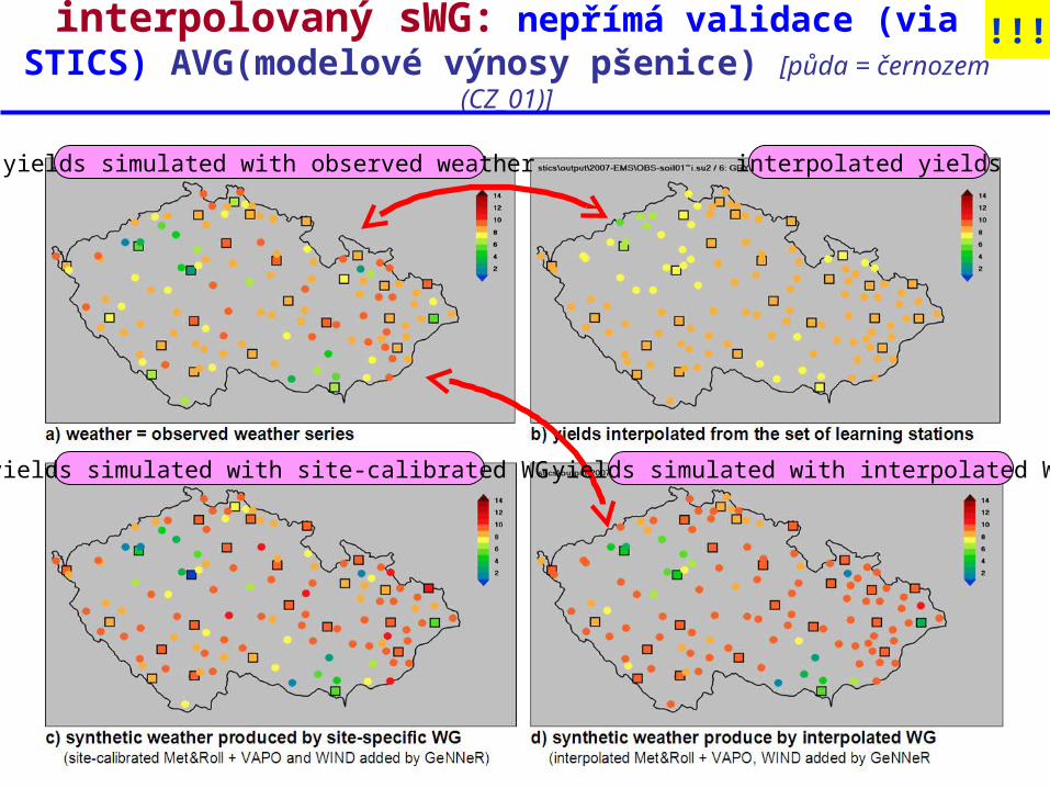
interpolovaný sWG: nepřímá validace (via STICS) AVG(modelové výnosy pšenice) [půda = černozem (CZ_01)]
interpolated yields
yields simulated with interpolated WGyields simulated with site-calibrated WG
yields simulated with observed weather
!!!
Scénáře změny klimatu
part 3
… s důrazem na nejistoty
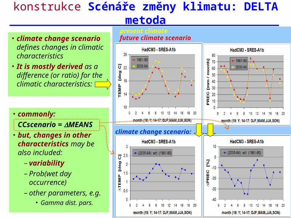
konstrukce Scénáře změny klimatu: DELTA metoda
• climate change scenario defines changes in climatic characteristics
• It is mostly derived as a difference (or ratio) for the climatic characteristics:
• commonly:
CCscenario = MEANS
• but, changes in other characteristics may be also included:
– variability
– Prob(wet day occurrence)
– other parameters, e.g.• Gamma dist. pars.
present climate future climate scenario
climate change scenario:

kaskáda nejistot při vývoji regionálního scénáře změny klimatu
1. emission scenario
carbon cycle & chemistry model
2. concentration of GHG and aerosols >> radiation forcing
GCM
3. large-scale patterns of climatic characteristics
downscaling
4. .....................................site-specific climate scenario
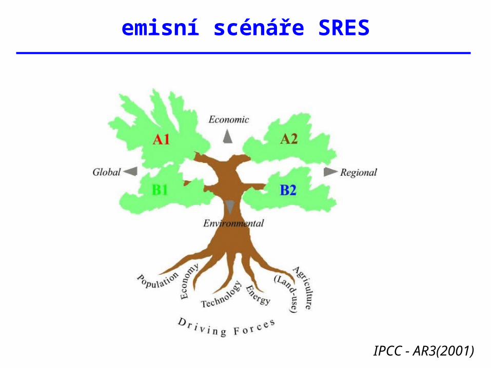
emisní scénáře SRES
IPCC - AR3(2001)
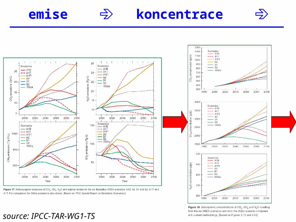
emise koncentrace
source: IPCC-TAR-WG1-TS
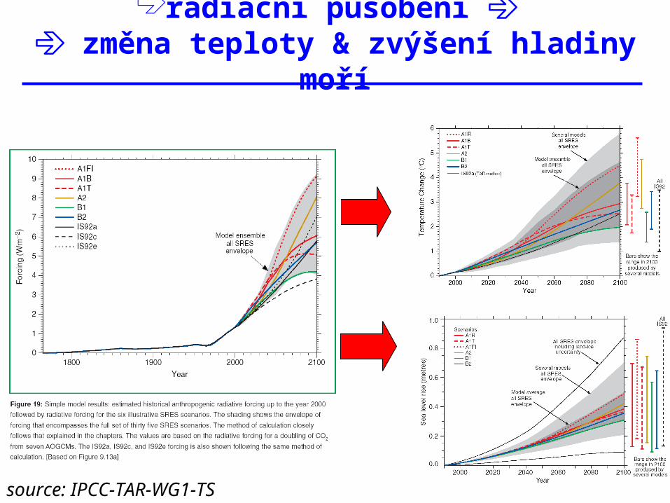
radiační působení změna teploty & zvýšení hladiny moří
source: IPCC-TAR-WG1-TS

naším cílem při studiu dopadů změny klimatu:
pravděpodobnostní vyhodnocení impaktů zohledňující známé nejistoty
For this, we need scenarios from
Several emission scenarios X several GCM simulations
(GCMs: various models, various settings, various realisations)
• … but: GCM simulations need huge computer resources- >> only limited number of GCM simulations available- >> GCM simulations do not cover existing uncertainties in emissions,
climate sensitivity)
• so, to account for the uncertainties, we may use:– http://www.climateprediction.net– pattern scaling, which separates global and regional uncertainties
zohlednění nejistot:
www.climateprediction.net
- distributed modelling
- anybody can participate
- based on Hadley Centre models
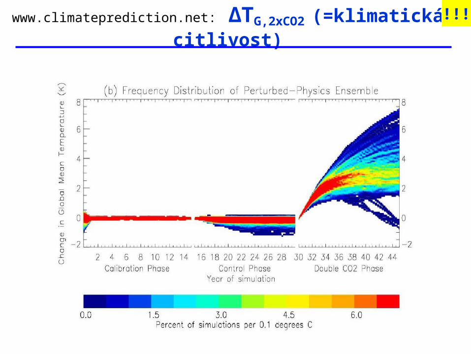
www.climateprediction.net: ΔTG,2xCO2 (=klimatická citlivost)!!!
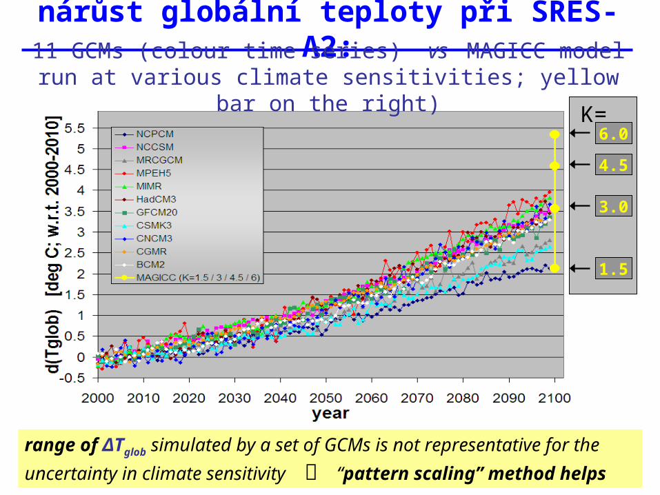
K=
nárůst globální teploty při SRES-A2:
1.5
3.0
4.5
6.0
range of ΔTglob simulated by a set of GCMs is not representative for the
uncertainty in climate sensitivity “pattern scaling” method helps
11 GCMs (colour time series) vs MAGICC model run at various climate sensitivities; yellow bar on the right)
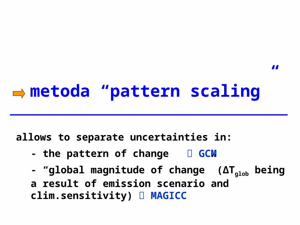
metoda “pattern scaling”
allows to separate uncertainties in:
- the pattern of change GCM
- “global magnitude of change” (ΔTglob being a result of emission scenario and clim.sensitivity) MAGICC
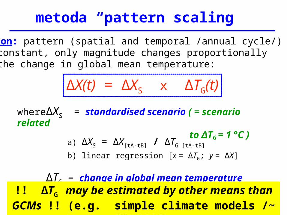
metoda “pattern scaling”
where ΔXS = standardised scenario ( = scenario relatedto ΔTG = 1 °C )
a) ΔXS = ΔX[tA-tB] / ΔTG [tA-tB]
b) linear regression [x = ΔTG; y = ΔX]
ΔTG = change in global mean temperature
assumption: pattern (spatial and temporal /annual cycle/)is constant, only magnitude changes proportionallyto the change in global mean temperature:
!! ΔTG may be estimated by other means than GCMs !! (e.g. simple climate models /~ MAGICC/)
ΔX(t) = ΔXS x ΔTG(t)
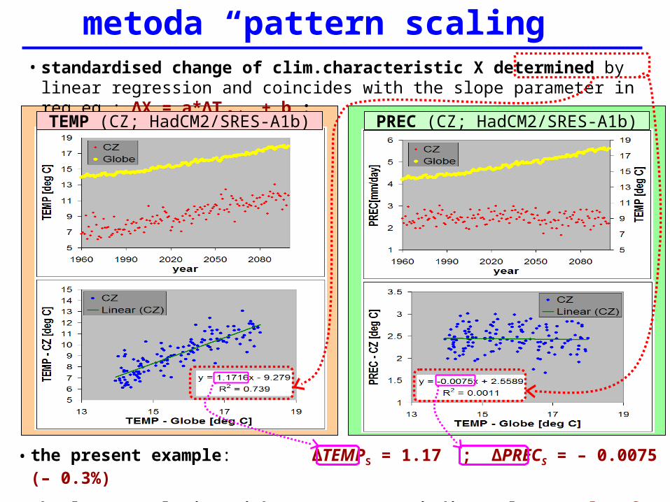
metoda “pattern scaling”• standardised change of clim.characteristic X determined by linear regression
and coincides with the slope parameter in reg.eq.: ΔX = a*ΔTglobe + b :
• the present example: ΔTEMPS = 1.17 ; ΔPRECS = – 0.0075 (– 0.3%)
• the low correlation with Tglobe (R2) may indicate large role of natural variability
TEMP (CZ; HadCM2/SRES-A1b) PREC (CZ; HadCM2/SRES-A1b)
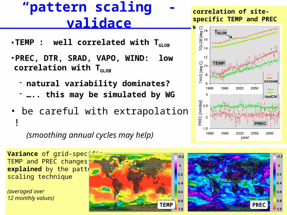
correlation of site-specific TEMP and PREC with TGLOB
Variance of grid-specificTEMP and PREC changesexplained by the patternscaling technique
(averaged over12 monthly values)
“pattern scaling” - validace
•TEMP : well correlated with TGLOB
•PREC, DTR, SRAD, VAPO, WIND: low correlation with TGLOB
natural variability dominates? ….. this may be simulated by WG
• be careful with extrapolation !(smoothing annual cycles may help)
TEMP PREC
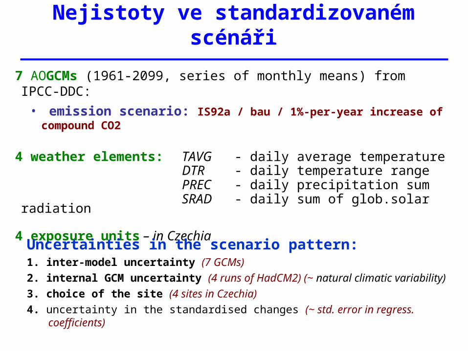
Nejistoty ve standardizovaném scénáři
7 AOGCMs (1961-2099, series of monthly means) from IPCC-DDC:
• emission scenario: IS92a / bau / 1%-per-year increase of compound CO2
4 weather elements: TAVG - daily average temperatureDTR - daily temperature rangePREC - daily precipitation sumSRAD - daily sum of glob.solar radiation
4 exposure units – in Czechia
Uncertainties in the scenario pattern:1. inter-model uncertainty (7 GCMs)
2. internal GCM uncertainty (4 runs of HadCM2) (~ natural climatic variability)
3. choice of the site (4 sites in Czechia)
4. uncertainty in the standardised changes (~ std. error in regress. coefficients)
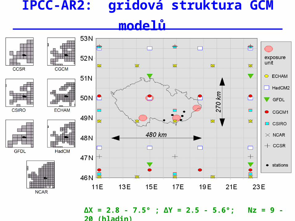
IPCC-AR2: gridová struktura GCM modelů
ΔX = 2.8 - 7.5º ; ΔY = 2.5 - 5.6º; Nz = 9 - 20 (hladin)
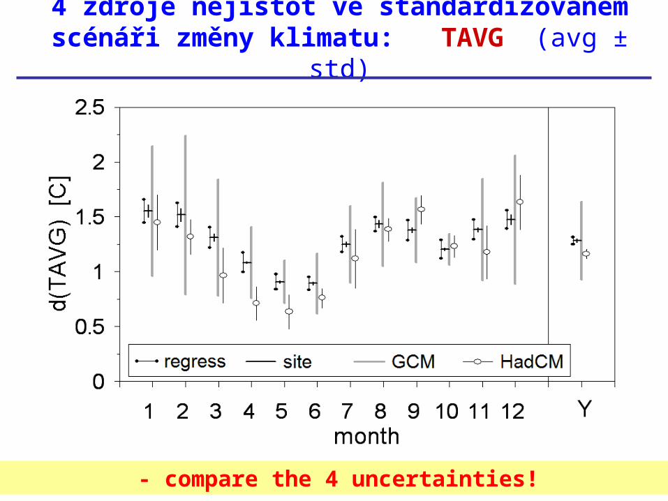
4 zdroje nejistot ve standardizovaném scénáři změny klimatu: TAVG (avg ± std)
- compare the 4 uncertainties!
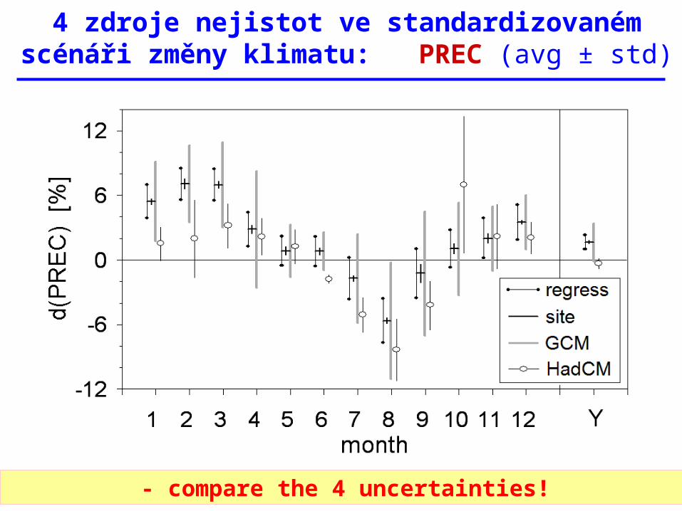
4 zdroje nejistot ve standardizovaném scénáři změny klimatu: PREC (avg ± std)
- compare the 4 uncertainties!
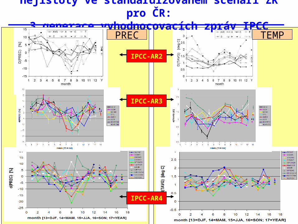
nejistoty ve standardizovaném scénáři ZK pro ČR:3 generace vyhodnocovacích zpráv IPCC
IPCC-AR4
PREC TEMP
IPCC-AR3
IPCC-AR2
nejistoty v modelech z IPCC-AR4
- - Evropa - -
[presented at EGU2009]
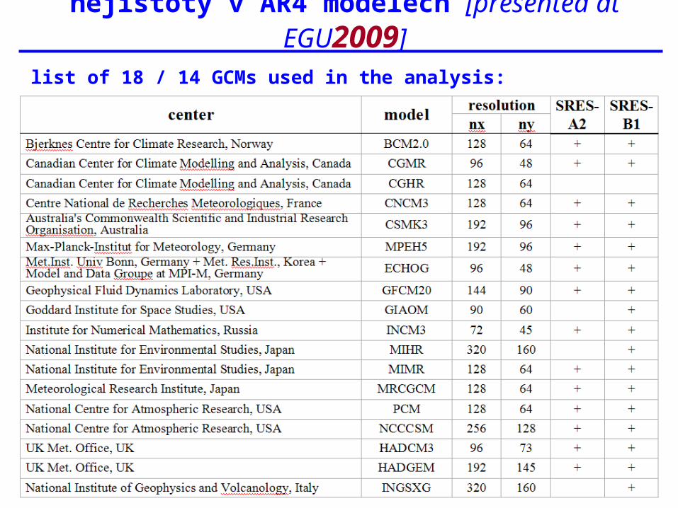
nejistoty v AR4 modelech [presented at EGU2009]
list of 18 / 14 GCMs used in the analysis:
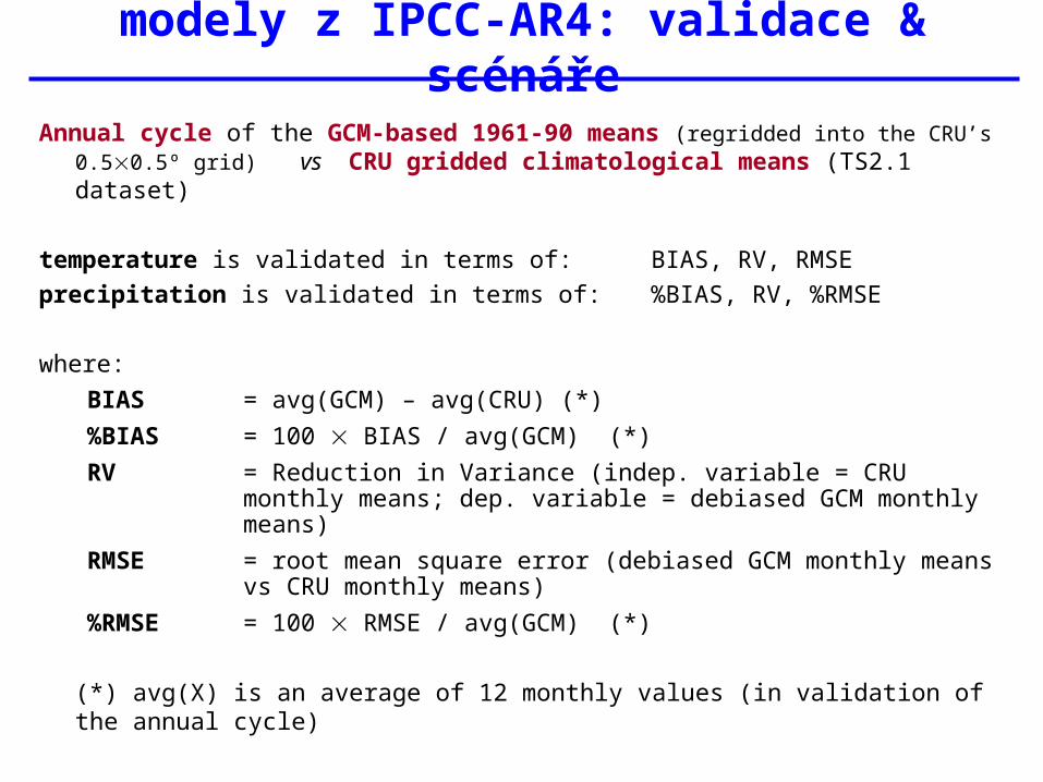
modely z IPCC-AR4: validace & scénáře
Annual cycle of the GCM-based 1961-90 means (regridded into the CRU’s 0.50.5º grid) vs CRU gridded climatological means (TS2.1 dataset)
temperature is validated in terms of: BIAS, RV, RMSE
precipitation is validated in terms of: %BIAS, RV, %RMSE
where:
BIAS = avg(GCM) – avg(CRU) (*)
%BIAS = 100 BIAS / avg(GCM) (*)
RV = Reduction in Variance (indep. variable = CRU monthly means; dep. variable = debiased GCM monthly means)
RMSE = root mean square error (debiased GCM monthly means vs CRU monthly means)
%RMSE = 100 RMSE / avg(GCM) (*)
(*) avg(X) is an average of 12 monthly values (in validation of the annual cycle)

GCMs vs CRU (1961-90 měsíční průměry)
RMSE(roční chod TAVG)
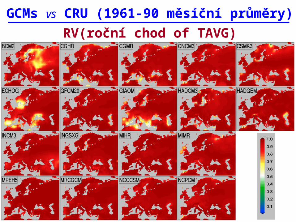
GCMs vs CRU (1961-90 měsíční průměry)
RV(roční chod of TAVG)
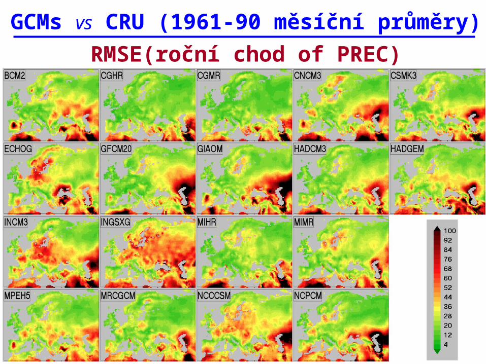
GCMs vs CRU (1961-90 měsíční průměry)
RMSE(roční chod of PREC)
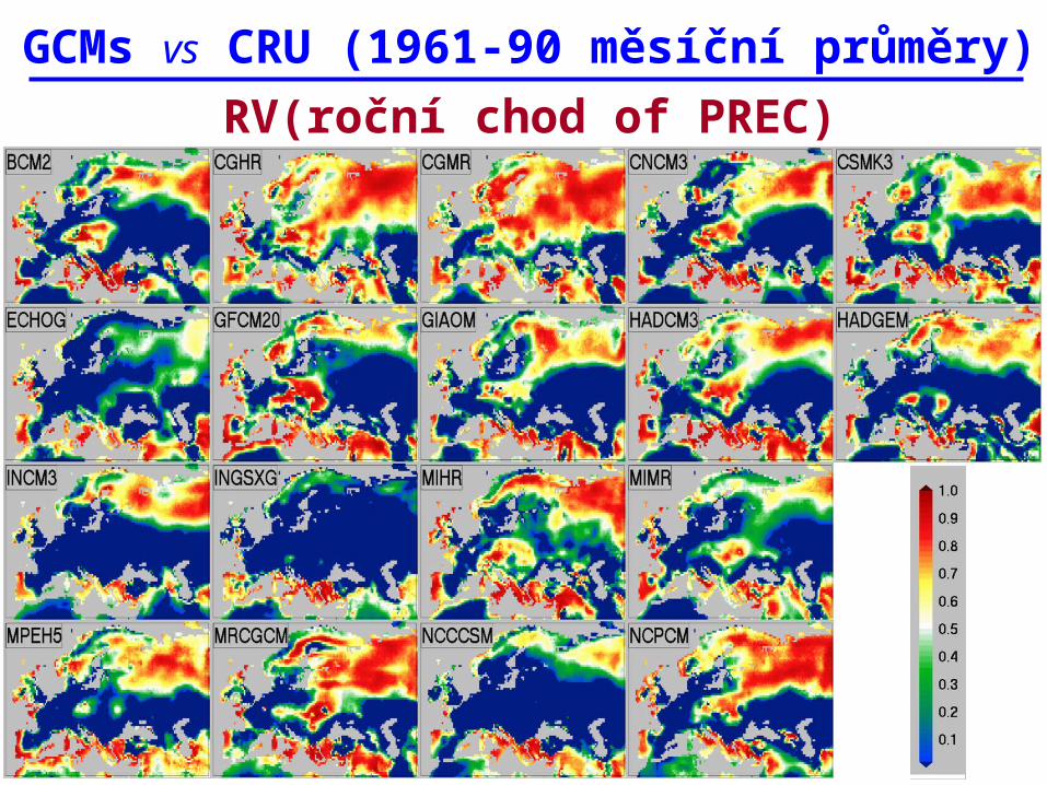
GCMs vs CRU (1961-90 měsíční průměry)
RV(roční chod of PREC)
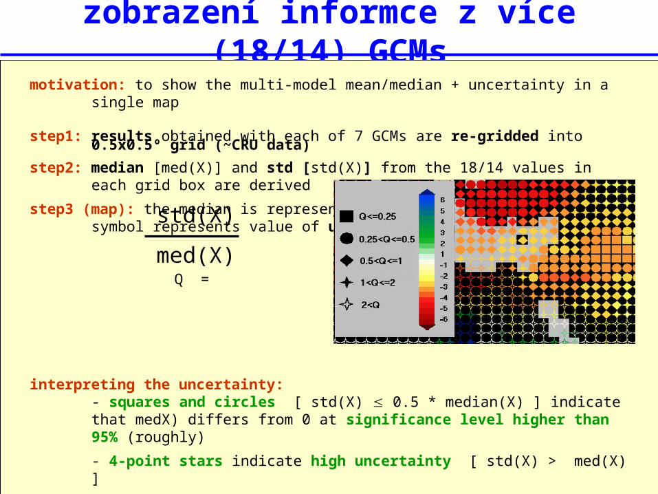
zobrazení informce z více (18/14) GCMs
motivation: to show the multi-model mean/median + uncertainty in a single map
step1: results obtained with each of 7 GCMs are re-gridded into 0.5x0.5º grid (~CRU data)
step2: median [med(X)] and std [std(X)] from the 18/14 values in each grid box are derived
step3 (map): the median is represented by a colour, the shape of the symbol represents value of uncertainty factor Q:
Q =
interpreting the uncertainty:- squares and circles [ std(X) 0.5 * median(X) ] indicate that medX) differs from 0 at significance level higher than 95% (roughly)
- 4-point stars indicate high uncertainty [ std(X) > med(X) ]
or: the greater is the proportion of grey (over sea) or black (over land) colour, the
lower is the significance, with which the median value differs from 0
std(X)
med(X)
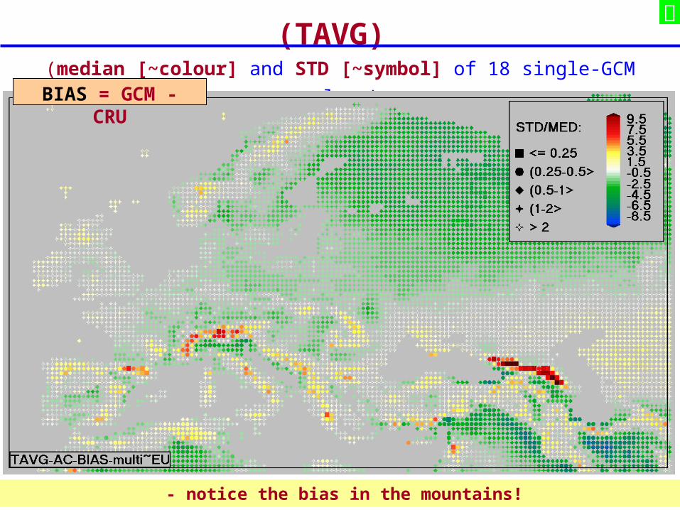
Multi-GCM validace: roční chod (TAVG) (median [~colour] and STD [~symbol] of 18 single-GCM values)
BIAS = GCM - CRU
- notice the bias in the mountains!
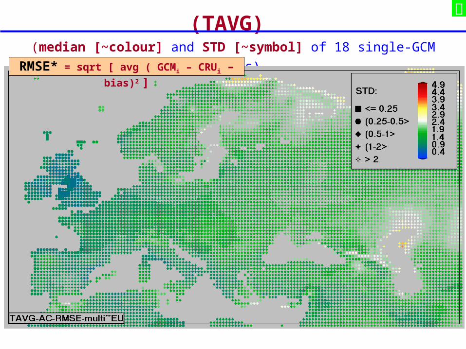
Multi-GCM validace: roční chod (TAVG) (median [~colour] and STD [~symbol] of 18 single-GCM values)
RMSE* = sqrt [ avg ( GCMi – CRUi – bias)2 ]
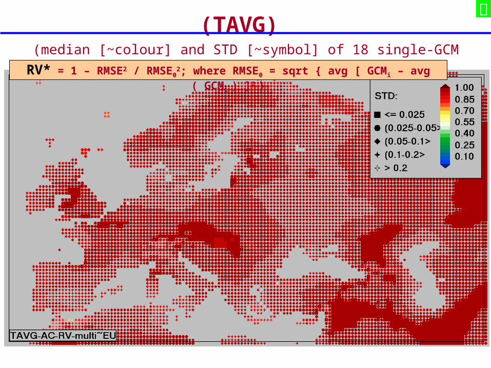
Multi-GCM validace: roční chod (TAVG) (median [~colour] and STD [~symbol] of 18 single-GCM values)
RV* = 1 – RMSE2 / RMSE02; where RMSE0 = sqrt { avg [ GCMi – avg ( GCMi ) ]2 }
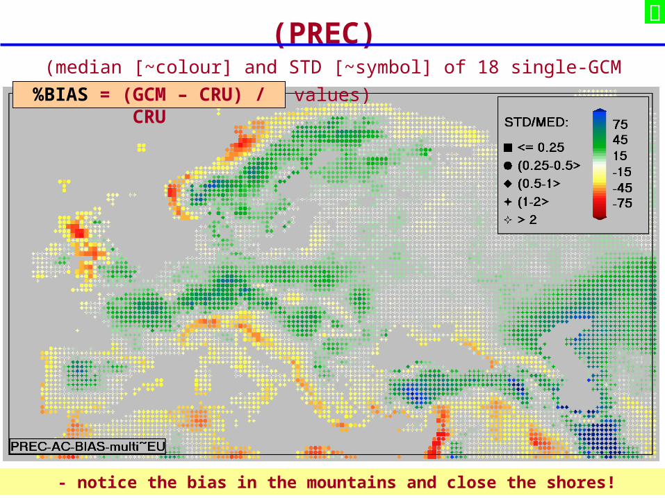
Multi-GCM validace: roční chod (PREC) (median [~colour] and STD [~symbol] of 18 single-GCM values)
%BIAS = (GCM – CRU) / CRU
- notice the bias in the mountains and close the shores!
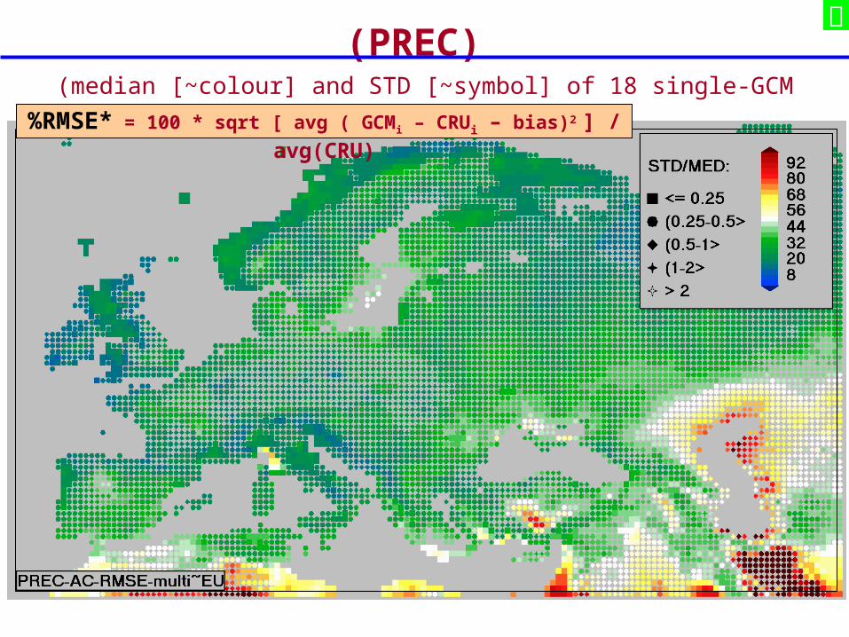
Multi-GCM validace: roční chod (PREC) (median [~colour] and STD [~symbol] of 18 single-GCM values)
%RMSE* = 100 * sqrt [ avg ( GCMi – CRUi – bias)2 ] / avg(CRU)
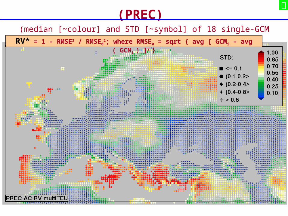
Multi-GCM validace: roční chod (PREC) (median [~colour] and STD [~symbol] of 18 single-GCM values)
RV* = 1 – RMSE2 / RMSE02; where RMSE0 = sqrt { avg [ GCMi – avg ( GCMi ) ]2 }
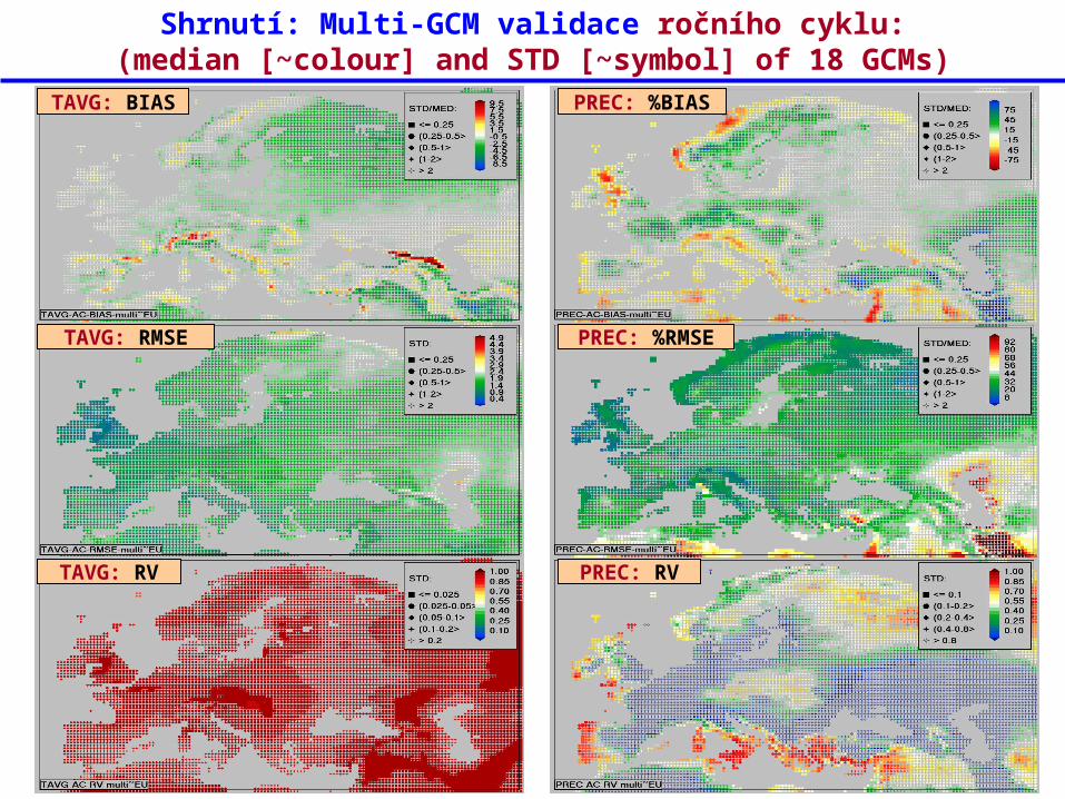
Shrnutí: Multi-GCM validace ročního cyklu:(median [~colour] and STD [~symbol] of 18 GCMs)
TAVG: BIAS
TAVG: RMSE
TAVG: RV
PREC: %BIAS
PREC: %RMSE
PREC: RV
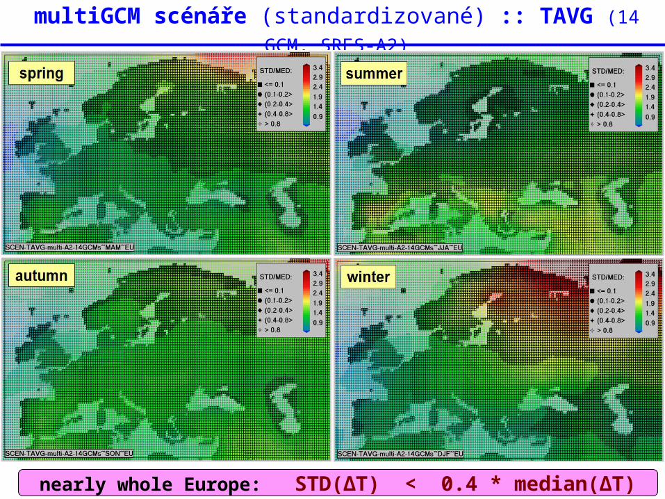
multiGCM scénáře (standardizované) :: TAVG (14 GCM, SRES-A2)
nearly whole Europe: STD(ΔT) < 0.4 * median(ΔT)
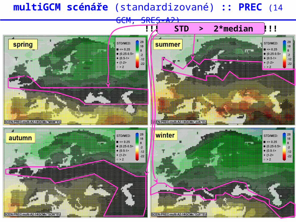
multiGCM scénáře (standardizované) :: PREC (14 GCM, SRES-A2)
!!! STD > 2*median !!!
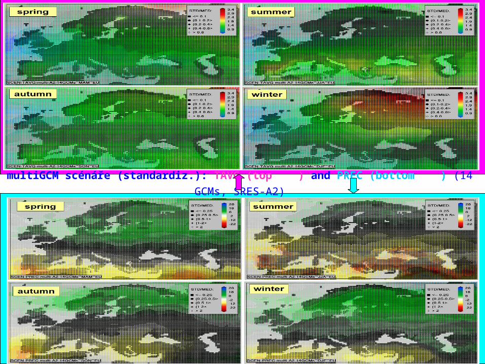
multiGCM scénáře (standardiz.): TAVG (top ) and PREC (bottom ) (14 GCMs, SRES-A2)

Konstrukcesady scénářů změny klimatu
pro impaktové studie
!!!
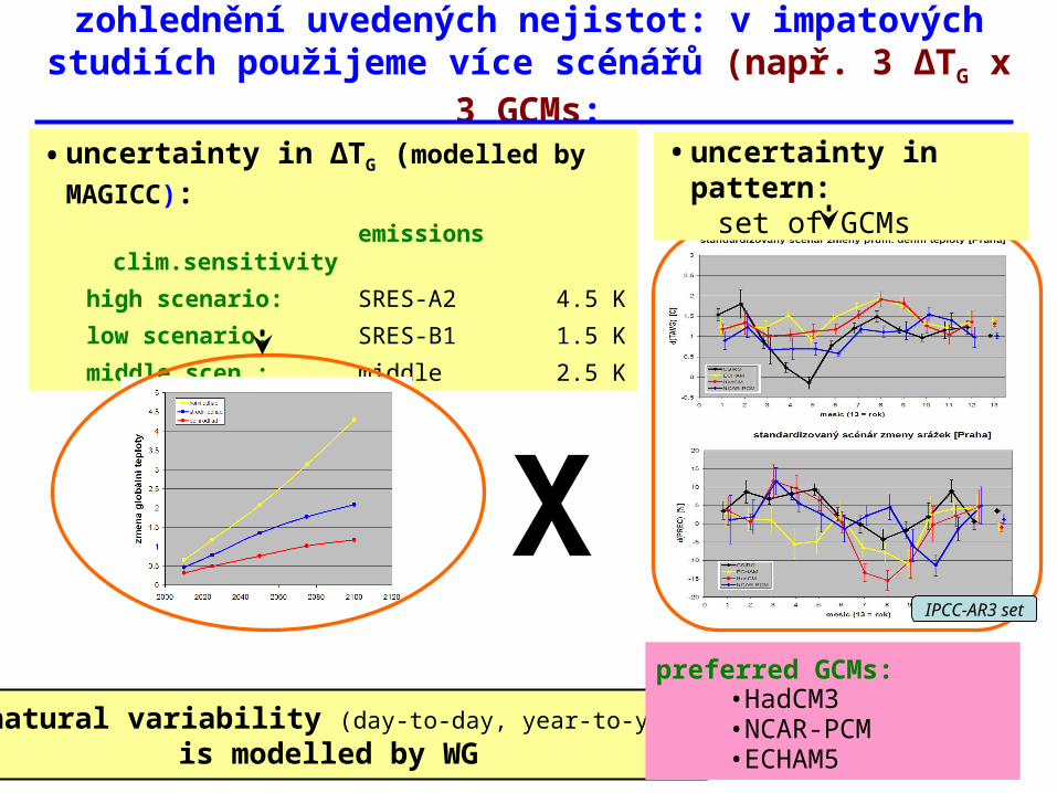
zohlednění uvedených nejistot: v impatových studiích použijeme více scénářů (např. 3 ΔTG x 3 GCMs:
• uncertainty in ΔTG (modelled by MAGICC):
emissionsclim.sensitivity
high scenario: SRES-A2 4.5 K
low scenario: SRES-B1 1.5 K
middle scen.: middle 2.5 K
XIPCC-AR3 set
• uncertainty in pattern: set of GCMs
+ natural variability (day-to-day, year-to-year)
is modelled by WG
preferred GCMs:•HadCM3•NCAR-PCM•ECHAM5
závěry
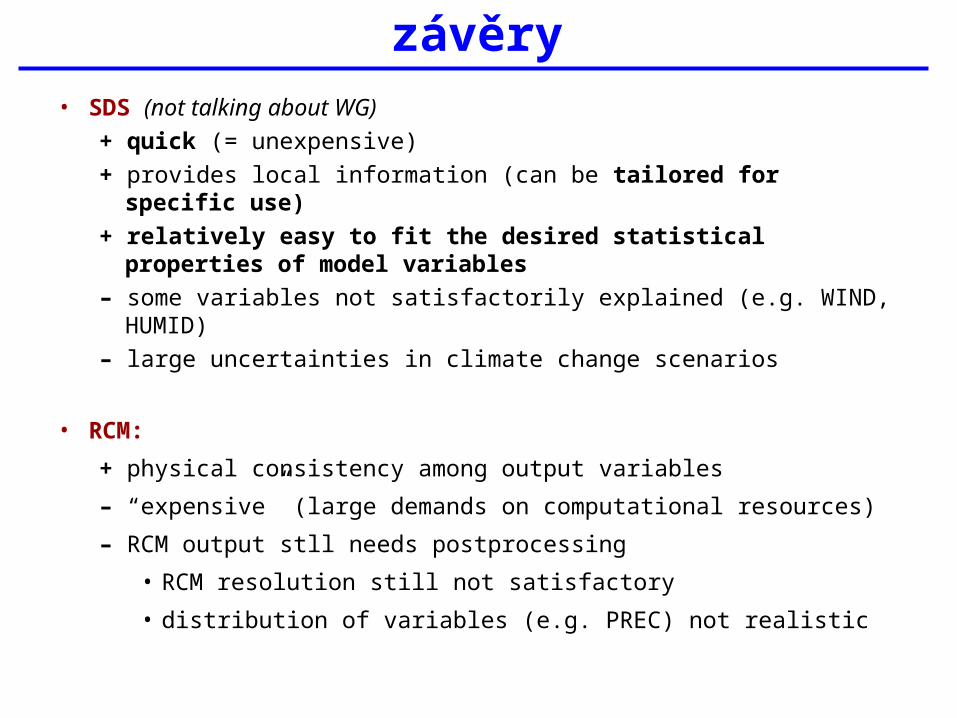
závěry• SDS (not talking about WG)
+ quick (= unexpensive)
+ provides local information (can be tailored for specific use)
+ relatively easy to fit the desired statistical properties of model variables
– some variables not satisfactorily explained (e.g. WIND, HUMID)
– large uncertainties in climate change scenarios
• RCM:
+ physical consistency among output variables
– “expensive” (large demands on computational resources)
– RCM output stll needs postprocessing
• RCM resolution still not satisfactory
• distribution of variables (e.g. PREC) not realistic
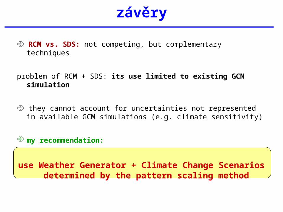
závěry
RCM vs. SDS: not competing, but complementary techniques
problem of RCM + SDS: its use limited to existing GCM simulation
they cannot account for uncertainties not represented in available GCM simulations (e.g. climate sensitivity)
my recommendation:
use Weather Generator + Climate Change Scenarios determined by the pattern scaling method
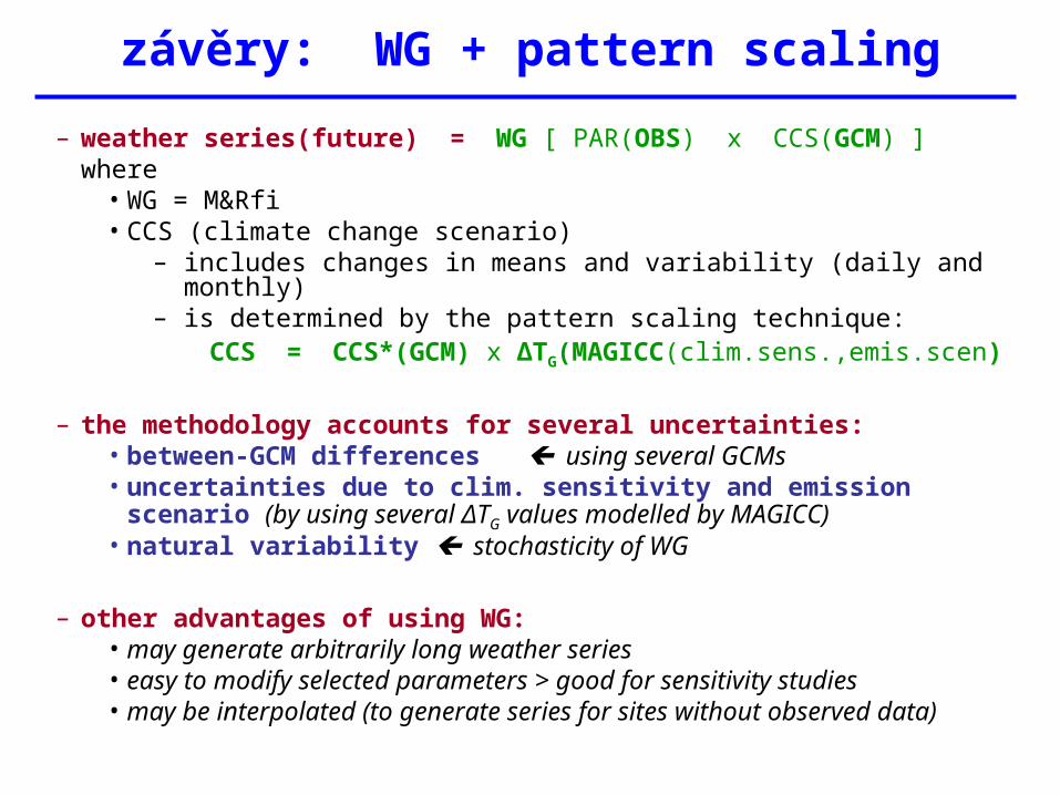
závěry: WG + pattern scaling
– weather series(future) = WG [ PAR(OBS) x CCS(GCM) ]where
• WG = M&Rfi• CCS (climate change scenario)
– includes changes in means and variability (daily and monthly)– is determined by the pattern scaling technique:
CCS = CCS*(GCM) x ΔTG(MAGICC(clim.sens.,emis.scen)
– the methodology accounts for several uncertainties:• between-GCM differences using several GCMs• uncertainties due to clim. sensitivity and emission scenario (by using
several ΔTG values modelled by MAGICC)• natural variability stochasticity of WG
– other advantages of using WG:• may generate arbitrarily long weather series• easy to modify selected parameters > good for sensitivity studies• may be interpolated (to generate series for sites without observed data)
k o n e c
více informací (+ prezentace na konferencích, články):
www.ufa.cas.cz/dub/crop/crop.htm