Methods to Mitigate Harmonics In Residential Power ... · The excessive waveform distortions in the...
119
University of Alberta Methods to Mitigate Harmonics In Residential Power Distribution Systems by Pooya Bagheri A thesis submitted to the Faculty of Graduate Studies and Research in partial fulfillment of the requirements for the degree of Master of Science in Energy Systems Department of Electrical & Computer Engineering ©Pooya Bagheri Spring 2013 Edmonton, Alberta Permission is hereby granted to the University of Alberta Libraries to reproduce single copies of this thesis and to lend or sell such copies for private, scholarly or scientific research purposes only. Where the thesis is converted to, or otherwise made available in digital form, the University of Alberta will advise potential users of the thesis of these terms. The author reserves all other publication and other rights in association with the copyright in the thesis and, except as herein before provided, neither the thesis nor any substantial portion thereof may be printed or otherwise reproduced in any material form whatsoever without the author's prior written permission.
-
Upload
hoanghuong -
Category
Documents
-
view
217 -
download
2
Transcript of Methods to Mitigate Harmonics In Residential Power ... · The excessive waveform distortions in the...

University of Alberta
Methods to Mitigate Harmonics
In
Residential Power Distribution Systems
by
Pooya Bagheri
A thesis submitted to the Faculty of Graduate Studies and Research in partial fulfillment of the requirements for the degree of
Master of Science in
Energy Systems
Department of Electrical & Computer Engineering
©Pooya Bagheri Spring 2013
Edmonton, Alberta
Permission is hereby granted to the University of Alberta Libraries to reproduce single copies of this thesis
and to lend or sell such copies for private, scholarly or scientific research purposes only. Where the thesis is
converted to, or otherwise made available in digital form, the University of Alberta will advise potential users
of the thesis of these terms.
The author reserves all other publication and other rights in association with the copyright in the thesis and,
except as herein before provided, neither the thesis nor any substantial portion thereof may be printed or
otherwise reproduced in any material form whatsoever without the author's prior written permission.
Abstract
The excessive waveform distortions in the present power distribution systems are
produced mainly by the large number of residential loads. Such distributed sources of
harmonics cannot be easily treated by the traditional mitigation methods, which have
been commonly applied for concentrated and easily detectable industrial distorting loads.
This thesis presents new harmonic mitigation techniques necessary for managing this
new situation. The proposed strategies are supported by several analytical and simulation
studies. Different options for both active and passive centralized and distributed filters
are investigated and compared to determine their different technical and economic
aspects. Overall, the results of extensive studies confirm that the novel zero-sequence
harmonic filter and the new scheme of the low-voltage distributed active filters
introduced in this thesis are promising solutions for the increasing harmonic problems in
residential feeders.

Acknowledgement
I would like to express my sincere appreciation to Dr. Wilsun Xu. This research and
dissertation would not have been possible without his guidance and great supervision. I
will always be proud to say I had the privilege of being his student, and I hope to have
learned enough to succeed in my future career.
I also thank my parents Hamid and Fatemeh for supporting me in so many different ways.
They supported my coming to Canada and my desire to spend another two years in
university for graduate studies. This is also extensive to my siblings, Nima, Shisa and
Mahsa, who have always loved me.

Contents
Chapter 1 Introduction..................................................................................... 1
1.1 Harmonics in Modern Distribution Systems............................................ 1
1.2 Traditional Mitigation Methods and the New Challenges ....................... 2
1.3 Harmonic Mitigation Objectives.............................................................. 3
1.4 Thesis Scope and Outline......................................................................... 5
Chapter 2 Harmonics Build-up in Modern Distribution Systems................ 8
2.1 Distribution Systems in North America ................................................... 9
2.2 Harmonic Modeling of Residential Loads ............................................... 9
2.3 Description of Studied Systems ............................................................. 10
2.4 Indices of Interest ................................................................................... 12
2.5 System-wide Harmonic Mitigation Objective........................................ 13
Chapter 3 Proposed Zero-Sequence Harmonic Filters................................ 15
3.1 Review on ZS Harmonic Filters............................................................. 15
3.2 Proposed Double-Tuned ZS Filter ......................................................... 17
3.3 Filter Construction & Design ................................................................. 20
3.4 Application Example.............................................................................. 22
3.4.1 Problem Description....................................................................... 23
3.4.2 Telephone Interference Mitigation Objective ................................. 23
3.4.3 Filter Location ................................................................................ 24
3.4.4 Filter Design Results....................................................................... 25
3.4.5 Filter Loading Assessment Results ................................................. 29
3.5 Conclusions ............................................................................................ 30
Chapter 4 Design of Medium-Voltage Passive Harmonic Filters............... 32
4.1 MV Passive Harmonic Filter Package ................................................... 32
4.2 Design Considerations............................................................................ 33
4.2.1 System Reactive Power Profile ....................................................... 33

4.2.2 Filter Components Loading ............................................................ 34
4.2.3 Filter Placement.............................................................................. 35
4.3 Overall Design Procedure ...................................................................... 36
4.4 Iterative Design Results ......................................................................... 39
4.4.1 For Ideal Feeder ............................................................................. 40
4.4.2 For Actual feeder ............................................................................ 45
4.5 Final Design Specifications.................................................................... 50
4.6 Summary ................................................................................................ 50
Chapter 5 Proposed Scheme for Low-Voltage Distributed Active Filters. 52
5.1 Filter Type and Topology Selection....................................................... 53
5.1.1 Active versus Passive Filters .......................................................... 53
5.1.2 Virtual-impedance Active Filter ..................................................... 54
5.2 Filter Installment Issues ......................................................................... 57
5.2.1 Double- phase Connection.............................................................. 57
5.2.2 Filter Location Options................................................................... 61
5.3 Simulation Studies on Secondary System.............................................. 63
5.3.1 Double-phase versus Single-phase Connection.............................. 66
5.3.2 Filter Placement in the Secondary System...................................... 67
5.3.3 Sensitivity Study of Filter Impedance ............................................. 71
5.4 Simulation Studies on Primary System.................................................. 71
5.4.1 Base Results .................................................................................... 72
5.4.2 Sensitivity Study of Feeder Parameters .......................................... 75
5.4.3 Sensitivity Study of Filter Impedance ............................................. 76
5.5 Final Design Specifications.................................................................... 78
5.6 Summary ................................................................................................ 79
Chapter 6 Comparison of Centralized and Distributed Filter Schemes.... 81
6.1 Mitigation Performance.......................................................................... 82
6.2 Technical Aspects Comparison.............................................................. 83
6.3 Economic Analysis................................................................................. 85
6.4 Summary ................................................................................................ 87

Chapter 7 Conclusions and Future Work..................................................... 88
7.1 Thesis Conclusions and Contributions................................................... 88
7.2 Suggestions for Future Work ................................................................. 89
References............................................................................................................ 91
Appendix.............................................................................................................. 96

List of Tables
Table 2.1 Main system parameters of the studied feeders. ...............................................12
Table 2.2 Conductor type, impedance and admittance of the feeder power-lines ............12
Table 3.1 C-message weighting factors for different harmonic frequencies ....................24
Table 3.2 The (ZS) filter impedance obtained by different sizes of transformers ............25
Table 3.3 Designed Components Size for the Single and Double-Tuned Filters .............26
Table 3.4 The adopted values of PEC-R and POSL-R for the loading assessment..................30
Table 4.1 List of transformers used for the filter design...................................................39
Table 4.2 The results of iterative filter design procedure for ideal feeder. .......................42
Table 4.3 Loading analysis of the designed filter for the ideal feeder. .............................44
Table 4.4 The results of iterative filter design procedure for actual feeder. .....................47
Table 4.5 Loading analysis of the designed filter for the actual feeder at neighborhood I.
..........................................................................................................................................49
Table 4.6 Loading analysis of the designed filter for the actual feeder at neighborhood II.
..........................................................................................................................................49
Table 4.7 Specification of designed MV passive filters for the system-wide harmonic
mitigation. .........................................................................................................................50
Table 5.1 Comparison of the two filter location options ..................................................63
Table 5.2 Simulation system parameters ..........................................................................66
Table 5.3 The harmonic reduction percentage for comparing filter locations A and B
including several cases with different length of lines and number of houses. ..................70
Table 5.4 The maximum allowable filter impedance values for different percentage of
secondary systems equipped with filters to accomplish the system-wide harmonic
mitigation objective in both of the real and ideal feeders. ................................................78
Table 5.5 The final design specifications of distributed active filters for a system-wide
harmonic mitigation in both the real and ideal feeders .....................................................79
Table 6.1 The proper filter type for the distributed and centralized schemes...................81
Table 6.2 Technical comparison between the two harmonic filter schemes.....................85
Table 6.3 Cost of capacitors and inductors for a MV filter. .............................................85
Table 6.4 Estimated costs for each MV filter installation.................................................86
Table 6.5 Estimated price of transformers (for the ZS filters).......................................... 86

Table 6.6 Overall estimated cost for components and installations of designed MV filter
packages............................................................................................................................86
Table 6.7 Comparison of total mitigation costs by the MV filters and the distributed
active filters.......................................................................................................................87
List of Figures
Figure 2.1 A generic schematic of a residential distribution feeder in North America. .....9
Figure 2.2 Schematic view of the ideal feeder circuit.......................................................11
Figure 2.3 Schematic view of the actual distribution feeder chosen for studies...............11
Figure 3.1 The conventional ZS harmonic filters: (a) zig-zag transformer-based (b) star-
type (c) star-type including a three-phase inductor...........................................................16
Figure 3.2 The transformer-based ZS filter topologies: (a) conventional single-tuned
version (b) proposed double-tuned version.......................................................................17
Figure 3.3 Zero-sequence frequency scan of the designed filters.....................................17
Figure 3.4 (a) The ZS filter (b) The equivalent ZS circuit of single-tuned ZS Filter (c)
The equivalent ZS circuit of the double-tuned ZS Filter ..................................................18
Figure 3.5 (a) Two paralleled conventional single-tuned filters (b) The conventional
double-tuned filter.............................................................................................................19
Figure 3.6 The flowchart of design procedure for the proposed ZS filters.......................22
Figure 3.7 The schematic view of the studied distribution feeder ....................................23
Figure 3.8 IDD of the dominant sequence of harmonic current components (daily 95%
percentile value)................................................................................................................27
Figure 3.9 The harmonic spectrum of induced voltage on the parallel conductor (daily
95% percentile value) .......................................................................................................28
Figure 3.10 C-message weighted voltage components induced on the parallel conductor
(daily 95% percentile value) .............................................................................................28
Figure 3.11 Daily profile of harmonic currents flowing inside the transformer (primary
side) of the designed ZS filters (a) at location ‘F1’ (b) at location ‘F2’. .........................29
Figure 3.12 Estimated daily profile of the transformer loading level (TLL) for the
designed ZS filters (a) at location ‘F1’ (b) at location ‘F2’ ..............................................30
Figure 4.1 The MV level passive filter package consisting of a double-tuned ZS filter and
the conventional single-tuned filter branches. ..................................................................33
Figure 4.2 Daily profile of real/reactive power profile of the actual feeder. ....................34
Figure 4.3 Daily profile of real/reactive power profile of the ideal feeder. ......................34
Figure 4.4 The proposed iterative design procedure in a quick view. ..............................36
Figure 4.5 Detailed flowchart of the proposed design procedure for the MV passive filter.
..........................................................................................................................................38

Figure 4.6. Votage IHD of both feeders average over feeder before filter installation
(daily 95% percentile value). ............................................................................................40
Figure 4.7 Current IDD of both feeders at the substation before filter installation (daily
95% percentile value). ......................................................................................................40
Figure 4.8 Positive-sequence frequency scans of the designed filter and system
impedance for ideal feeder................................................................................................43
Figure 4.9 Zero-sequence frequency scans of the designed filter and system impedance
for ideal feeder. .................................................................................................................44
Figure 4.10 Daily voltage profile at the middle of the ideal feeder. .................................45
Figure 4.11 Daily voltage profile at the end of the ideal feeder .......................................45
Figure 4.12 The MV filters locations in the actual feeder ................................................46
Figure 4.13 Positive-sequence frequency scans of the designed filter and system
impedance for actual feeder. .............................................................................................48
Figure 4.14 Zero-sequence frequency scans of the designed filter and system impedance
for actual feeder. ...............................................................................................................48
Figure 4.15 Daily voltage profile at Neighbourhood I......................................................48
Figure 4.16 Daily voltage profile at Neighbourhood II. ...................................................48
Figure 5.1 A generic residential distribution feeder illustrating different possible filter
schemes.............................................................................................................................52
Figure 5.2 Simplified schematic of a shunt active filter with (a) current-detection based
control (traditional type) (b) voltage-detection based control (virtual-impedance). .........55
Figure 5.3 Frequency scan at a house of a typical secondary feeder (House #3 in Figure
5.11) ..................................................................................................................................56
Figure 5.4 The single-phase virtual-impedance active filter (a) Circuit schematic and
control diagram (b) Equivalent system .............................................................................57
Figure 5.5 Different possible filter installment options: (b) Two single-phase connected
filters (c) One double-phase connected filter. ...................................................................58
Figure 5.6 Equivalent circuit of system with (a) two single-phase filter (b) one double-
phase filter.........................................................................................................................58
Figure 5.7 The two options for filter location: (a) at service transformer (b) at one of the
houses................................................................................................................................61
Figure 5.8 The equivalent circuit of system when installing filter at one of the houses...61
Figure 5.9 The equivalent filter branch when installing filter at one of the houses,
simplified with ignoring the harmonic currents generated inside that house.................... 62

Figure 5.10 Different configurations of a secondary distribution system (a) cascade (b)
parallel (c) combination of parallel and cascade...............................................................63
Figure 5.11 The typical secondary system chosen for simulation studies. .......................64
Figure 5.12 The model circuit of the secondary system at fundamental frequency for
harmonic load flow simulations........................................................................................65
Figure 5.13 The model circuit of the secondary system at harmonic frequencies for
harmonic load flow simulations........................................................................................65
Figure 5.14 Comparison of single-phase and double-phase filter configurations in
mitigation of harmonic currents penetrating the primary system (a) Daily profile of
Current TDD (b) Daily average value IDD. .....................................................................67
Figure 5.15 Harmonic current daily profile for different filter locations..........................68
Figure 5.16 Daily average harmonic current IDD for different filter locations................68
Figure 5.17 A generalized secondary distribution system with a combined parallel-
cascade configuration........................................................................................................69
Figure 5.18 Percentage decrease of daily average current TDD obtained with different
filter impedance values. ....................................................................................................71
Figure 5.19 Current TDD in substation (daily 95% percentile value) versus percentage of
service transformers equipped with distributed filters. .....................................................73
Figure 5.20 Voltage THD (daily 95% percentile value) average along feeder versus
percentage of service transformers equipped with distributed filters. ..............................73
Figure 5.21 Percentage decrease of substation current TDD versus percentage of
secondary systems equipped with the distributed filters installed in service transformer.74
Figure 5.22 Percentage decrease of feeder average voltage THD versus percentage of
secondary systems equipped with the distributed filters installed in service transformer.75
Figure 5.23 Percentage decrease values of current TDD and voltage THD versus
percentage of service transformers equipped with distributed filters for different feeder
characteristics....................................................................................................................76
Figure 5.24 Percentage decrease of current TDD and voltage THD versus filter
impedance including four different percentages of service transformers equipped with
virtual-impedance distributed filters (a) (b) Ideal feeder (c)(d) Actual feeder (The filters
are installed directly at service transformers for all the cases). ........................................77
Figure 6.1 Daily maximum voltage IHD average over the feeder for the MV and
distributed filters cases in the ideal feeder. .......................................................................82
Figure 6.2 Daily maximum current IDD in substation for the MV and distributed filters
cases in the ideal feeder. ...................................................................................................82
Figure 6.3 Daily maximum voltage IHD average over the feeder for the MV and
distributed filters cases in the actual feeder. .....................................................................83
Figure 6.4 Daily maximum current IDD in substation for the MV and distributed filters
cases in the actual feeder...................................................................................................83
Chapter 1. Introduction
1
Chapter 1
Introduction
Harmonic distortion has been always one of the major concerns in the area of electrical
power quality. Because of their potential negative impacts, the uncontrolled flow of
harmonics in power systems has been always prevented by employing various mitigation
methods. Traditionally, the dominant harmonic sources were usually associated with
some industrial loads at known locations. Then, in most cases, the customers with the
major distorting loads were asked to install harmonic filters, which prevented the
excessive harmonic distortions from entering the supply system. Standards and guidelines
have been developed in the literature to plan effective mitigation measures to control the
harmonic distortions in such situations [1]- [3]. Therefore, the power utility companies
have successfully managed to supply the nonlinear loads of industrial customers without
any noticeable issue.
However, after the start of the 21st century and the widespread penetration of modern
nonlinear electronic devices into the regularly used home appliances, the nature of
harmonic sources has significantly changed. From the easily detectable concentrated
loads of the past, the major harmonic sources have evolved into several small ones
dispersed throughout the whole distribution system. This trend has raised serious
concerns regarding the capability of the traditional methods to manage this new harmonic
situation. This introductory chapter presents an overview of the harmonics in the modern
distribution systems. Then, the traditional mitigation methods are reviewed. Next, the
need to develop new techniques is discussed. Finally, this chapter presents the scope and
outline of this thesis.
1.1 Harmonics in Modern Distribution Systems
Several modern home appliances such as compact fluorescent lights, LCD TVs and
personal computers generally inject a large amount of harmonic currents into their supply
systems. The massive growth in usage of such energy-efficient consumer electronic
devices has resulted in significant distortions to the voltage and current waveforms in the

Chapter 1. Introduction
2
present power distribution systems. Although each of the devices is not individually a
large source of harmonics, the collective effect is so noticeable that the excessive
waveform distortions in urban distribution systems are becoming increasingly dominated
by the harmonics of residential loads [4]- [7].
The high levels of harmonic distortion in a power system increase the risk of different
troublesome and unwelcome effects. For example, several serious problems associated
with the harmonics of residential feeders (telephone interference is the most common
problem) have been recently experienced by the utility companies in Alberta, Canada.
Because of their energy-saving feature, nonlinear electronic devices will probably
continue their rapid penetration into the power systems and possibly cause a severe
harmonic situation in the near future.
The uniqueness of this new harmonic condition raises serious doubts and concerns
regarding the effectiveness of the existing standards and practices for managing and
mitigating the distortions in the present distribution systems. As a result, research on
advanced and efficient mitigation methods which can be properly planned in accordance
with the new characteristics of the modern harmonic sources is obviously needed.
1.2 Traditional Mitigation Methods and the ew Challenges
Traditionally, specific industry customers known to the utilities possessed the dominant
harmonic sources. Consequently, the harmonic problems were identified and treated by
installing passive harmonic filters at the Point of Common Coupling (PCC) of the major
distorting loads so that the filter effectiveness was easily assessed and verified [3], [8]-
[10]. However, the situation becomes quite complicated with the presence of harmonic-
generating residential loads. Such small harmonic sources are widely and randomly
dispersed across the system.
Several researches have tried to develop possible mitigation measures for this new
situation. For Medium-Voltage (MV) applications, shunt passive harmonic filters are
generally the most popular solution for harmonic problems in the power industry, due to
these filters reasonable cost and reliability [11], [12]. Therefore, various design methods
have been proposed and developed in the literature for installing passive harmonic filters
to mitigate the dispersed harmonic sources in a distribution feeder [13]- [15]. Moreover,

Chapter 1. Introduction
3
complex optimization algorithms have been also developed for placing the filters when
the distorting loads are distributed along the feeder [15]- [17]. Nonetheless, the treatment
of distributed harmonic sources is still challenged by several difficulties such as the lack
of a practical and comprehensive technique of filter design and placement. For instance,
the proposed passive filter designs in the literature vary from case to case, depending on
the feeder characteristics. Moreover, in order to mitigate all the harmonic orders (3rd, 5th,
7th, etc.) several passive filter branches will be needed, and this requirement will
increases the implementation cost. As well, severe harmonic amplifications caused by the
parallel resonance between the passive filters and the system are always possible
[12], [18]. Most of the issues associated with the shortcomings of passive filters can be
addressed by employing active harmonic filters [19], [20], but they have never been a
popular choice in industry practices, due to their high cost and insufficient reliability in
the MV-level applications.
Another unique characteristic of the harmonics associated with residential loads
involves the Zero-Sequence (ZS) harmonics. Unlike the industrial loads, most of the
residential loads are single-phase. This fact leads to the creation of ZS harmonic currents
in three-phase distribution systems. High levels of ZS harmonics are often observed in a
distribution system feeding residential loads nowadays. These harmonics can add up in
the neutral conductor, creating problems such as neutral voltage/current raise [21], [22].
They are also the main culprit of interference problems with the adjacent telephone lines
[23], [24]. Because ZS harmonics may also lead to problems similar to those caused by
positive- or negative-sequence harmonics, the excessive ZS harmonic distortions can be
problematic in a distribution system. Therefore, the ZS harmonics must be considered
when researching the harmonic mitigation solutions for modern residential feeders.
1.3 Harmonic Mitigation Objectives
In general, excessive harmonic distortions in a distribution system can cause several
problems such as the following [1], [2], [25]:
• Electromagnetic interference with adjacent telephone lines [26]
• Transformers or capacitor banks overheating
• Premature ageing of the insulation of the electrical plant components
• Errors in metering devices or malfunction of sensitive electronic devices
Chapter 1. Introduction
4
• Neutral overheating or voltage rise [21], [22]
• High level of harmonic penetration into the power transmission systems
In order to manage the risks and hazards associated with the problems listed above,
harmonic mitigation strategies are essential for both solving the existing problems and
preventing potential problems in future. In other words, the main objectives in planning
to mitigate harmonics in a distribution feeder can be classified into the following two
categories.
1) Mitigating a single-point problem: In this category, the mitigation measures are
used for a specific problem (such as one of those listed above) which has already
occurred in a system due to the high level of harmonic distortions. For example, the ZS
harmonics in a section of a feeder may have caused interference with its adjacent
telephone lines, or a capacitor bank in the system might be overloaded by extra amounts
of harmonics. In such cases, the problem will be approached with a specific mitigation
objective focused only on the troublesome harmonic components in the affected location.
For example, in a telephone interference case, filtering the ZS harmonics in the involved
power-line sections will be sufficient to solve the problem.
2) System-wide harmonic mitigation: In this approach, the purpose is to suppress the
harmonic distortions throughout the whole system to reduce the possibility of any
harmonic-caused problem in the future, thereby ensuring the system’s safe operation.
Moreover, all of the system’s sensitive devices such as the metering devices will also
benefit from the distortion-free voltage/current waveforms. Besides, the amount of
harmonics penetrated into the transmission systems is also controlled and the power
losses associated with harmonics are avoided as well by this approach.
This thesis proposes new methods and conducts studies to address the technical needs
and implementation issues associated with achieving both of these harmonic mitigation
approaches in a residential distribution system. For example, a thorough design guideline
is developed to mitigate the single-point problems caused by the ZS harmonics. The
thesis also introduces and investigates methods for accomplishing system-wide harmonic
mitigation in a distribution system.

Chapter 1. Introduction
5
1.4 Thesis Scope and Outline
The scope of this thesis is to develop thorough and effective methods for mitigating the
harmonics produced by the residential loads in a distribution feeder. Most of the past
research in the field of harmonic suppression focused only on the lumped, large and
known industrial loads. However, the harmonic distortions in the modern distribution
systems are dominated by the large number of randomly dispersed sources associated
with residential loads. Hence, new issues and concerns challenge the management of the
new harmonic situation. Some of the key questions that this thesis is aimed to answer are
as follows.
1. What are the unique characteristics of the residential distorting loads? Which
aspects of the traditional mitigation methods must be improved and extended to become
effective for such modern harmonic sources?
2. What are the effective methods to manage the high levels of ZS harmonics
emerging in the residential distribution feeders?
3. How can system-wide harmonic mitigation in a feeder serving residential customers
be achieved? What is the role of passive and active harmonic filters in this context? What
are the proper sizing and design methods?
4. Where should the harmonic filters be located in a system with dispersed harmonic
sources? Should either several distributed small filters or a few centralized bulky filters
be used? Which solution is more cost-effective? What are each method’s technical
advantages?
5. Can the filters be installed in the low-voltage secondary levels of the distribution
systems as well? If so, what are the advantages and challenges associated with such a
scheme?
In order to address the concerns highlighted in the above questions, this thesis
introduces several new methodologies and also conducts supporting technical studies.
The following paragraphs summarize the organization of the thesis and describe the main
topics and research discussed in each chapter.

Chapter 1. Introduction
6
Chapter 2 reviews the overall process of harmonic build-up in a modern residential
distribution system. The main characteristics of the North American distribution feeders
that affect the present harmonic situation are also discussed. The two systems used to
examine different mitigation schemes are also introduced in this chapter. The chapter
also discusses the modeling techniques employed in this thesis to develop a
comprehensive platform for all of the simulation studies. The models are used in the later
chapters to perform several Harmonic Load Flow (HLF) studies to assess the efficiency
of the different harmonic mitigation strategies.
Chapter 3 presents a novel technique to mitigate ZS harmonics in power distribution
systems. The method is based on the concept of passive ZS harmonic filters including
Yg/∆ transformers. However, its basic configuration has been expanded to create a
double-tuned filtering feature. This feature makes it possible to trap two ZS harmonics
with only one filter and is especially attractive for solving harmonic-caused telephone
interference problems. A method for sizing and loading assessment of the filter is also
proposed in this chapter. As sample application, the proposed filter package is applied to
mitigate a telephone interference problem. Issues such as filter location, the number of
filters required and the effectiveness of filtering ZS harmonics produced by distributed
residential loads are also investigated in this chapter.
As discussed earlier, a comprehensive and practical methodology for designing
passive MV filters to mitigate harmonics produced by the dispersed residential loads is
still unavailable. Chapter 4 develops a simplified design guideline for MV filter
applications for treating the modern harmonic situation. All of the special characteristics
of distributed harmonic sources are considered in the design process. In this chapter, the
final MV passive filter packages are sized for both of the studied systems.
Since the harmonic sources are dispersed in a residential feeder, the harmonic filters
can be also distributed all over the system. Indeed, instead of a bulky centralized filter in
the primary feeder, several small low-voltage filters can be installed in the secondary
levels of a distribution system. Chapter 5 presents a novel mitigation scheme based on
low-voltage distributed active filters. In each secondary system, the filters can either be
attached to the service transformer or configured as a meter collar inserted into the
revenue meter socket of one of the customers. Various analytical and simulation studies
Chapter 1. Introduction
7
are conducted in this chapter to develop the proper specifications and requirements of
such a filtering scheme in order to achieve an effective system-wide harmonic mitigation.
Chapter 6 presents a comprehensive comparison between the MV passive filter
solution (discussed in Chapter 4) and the distributed active filter scheme (introduced in
Chapter 5). The economic issues and the technical aspects are considered to identify the
strategy with the most overall advantages.
Finally, this thesis’s main conclusions and suggestions for future research in this field
are summarized in Chapter 7.

Chapter 2 . Harmonics Build-up in Modern Distribution Systems
8
Chapter 2
Harmonics Build-up in Modern Distribution Systems
The first critical step in planning an effective harmonic mitigation strategy is to correctly
understand and characterize the harmonic sources. Technically speaking, proper system
models and theoretical principles are required to formulate and quantify the harmonic
situation in the system. After such models and principles have been developed, effective
mitigation measures can be proposed and assessed. As discussed earlier, this task can be
quite challenging for researchers studying modern distribution systems where the
dominant sources of distortion are the large number of nonlinear residential appliances.
Such harmonic sources have a random and time-varying nature and unlike traditional
lumped and large harmonic loads, are dispersed all over a system. Traditionally, a set of
data consisting of the harmonic spectrum of the distorting load and the system
characteristic at the PCC (including system harmonic impedances and background
harmonics) was sufficient to conduct a harmonic filter design and study. However,
defining such a simple set of data is not possible for the modern situation where several
harmonic sources are dispersed in the system, and no single connecting point can be
identified as the PCC.
As a result, the first essential step is to establish theoretical principles and system models
that properly formulate and represent such modern sources of harmonic pollution.
Recently, researchers at the PDS lab at University of Alberta, Canada developed a
comprehensive simulation platform to represent distributed harmonic sources in a
residential power system [6], [7], [27], [28]. This thesis employs those models and
simulation techniques which are developed based on a bottom-up approach to quantify
the harmonic build-up in the residential feeders. After developing the required models, an
in-house Harmonic Load Flow (HLF) program [29] is used to perform simulations for
different case studies to examine the proposed mitigation strategies.
This chapter is organized as follows. Section 2.1 describes the general characteristics
of the power distribution systems in North America. Section 2.2 explains the bottom-up
modeling approach employed for performing HLF simulations in a residential feeder. The
parameters and characteristics of the selected feeders for conducting this thesis’s studies

Chapter 2 . Harmonics Build-up in Modern Distribution Systems
9
are given in section 2.3. Section 2.4 lists the main harmonic indices of interest used in
this thesis to evaluate different harmonic mitigation methods. Finally, section 2.5
establishes a precise mitigation objective that will be used as the design criteria to
develop system-wide harmonic suppression plans in Chapter 4 and Chapter 5.
2.1 Distribution Systems in orth America
Figure 2.1 shows a typical schematic of a North American distribution system supplying
residential loads. The system is consisting of the primary and secondary feeders. The
primary feeder transfers the electrical power from substation to several service
transformers. Each secondary system consists of a service transformer and the various
houses supplied by it. As shown in the figure, the houses are connected to 120V voltage
level of the service transformers through the secondary conductors.
Figure 2.1 A generic schematic of a residential distribution feeder in North America.
Nonlinear home appliances inside the houses are the major harmonic sources in this
system. As illustrated by the red flash arrows in the figure, each residential customer
injects a portion of harmonics to the system which penetrate to the primary feeder and
finally flows toward the substation.
2.2 Harmonic Modeling of Residential Loads
For the studies conducted in this thesis, the residential harmonic sources are quantified
and modeled employing the bottom–up probabilistic approach introduced in
[6], [7], [27], [28]. This method provides aggregated harmonic load models for the
distribution service transformers inside a feeder supplying residential houses. The
modeling technique can be summarized in the following steps [7], [28]:

Chapter 2 . Harmonics Build-up in Modern Distribution Systems
10
1) The types of regularly used electrical home appliances by the customers in the
study area are recognized.
2) The number of appliances per each household is estimated.
3) The probabilistic switch-on daily profile for each type of appliances is established
based on their typical daily usage patterns.
4) The model is developed for different times during a day. For each time snapshot,
appliances that are ON are modeled as the constant power loads in the fundamental
frequency and for the harmonic frequencies; current sources are used to model nonlinear
loads, whereas linear appliances are represented by impedances.
5) The aggregated harmonic model for a residential house is built.
6) The residential houses are connected to the secondary system models.
In order to reduce the complexity and computation time duration of primary system
simulations, it is essential to establish equivalent models for each secondary system
supplied by the feeder [28]. Based on a similar method as in [28], the equivalent models
are generated and verified, then, each group of a service transformer and its supplied
residential houses are substituted by their equivalents in the system model. ( Appendix A
explains the details of developing the aggregated models). Multiphase PI models are used
for all of the overhead lines and underground cables (including the single and double-
phase ones as well) inside the feeder. Neutral wire is also included by employing
multiphase models [28]. Finally, the developed models are employed in an In-House
multiphase HLF program [29] to perform the simulation studies. As the models are time-
varying during a day, the obtained results are for different times of the day.
2.3 Description of Studied Systems
The harmonic mitigation studies of this thesis are conducted on two distribution
systems as follows.
a) An ideal system supplying residential loads which are evenly distributed along the
feeder. This system can represent the generic characteristics of residential distribution
systems and will be referred as the ‘ideal feeder’ in this thesis.

Chapter 2 . Harmonics Build-up in Modern Distribution Systems
11
Figure 2.2 Schematic view of the ideal feeder circuit
b) An actual distribution feeder supplying some residential customers operated by a
utility company in Edmonton, Canada. The excessive harmonic distortions in this feeder
have caused some severe problems such as telephone interference. As shown in Figure
2.3, this feeder is supplying two large residential neighborhoods in the south areas of
Edmonton (encompassed by the circles in the figure) and will be referred as the ‘actual
feeder’ in this thesis. By including such system in the study platforms, the effectiveness
of the proposed mitigation schemes can be also examined for the real-world applications.
Figure 2.3 Schematic view of the actual distribution feeder chosen for studies.
The main characteristics and parameters of these two systems are given in Table 2.1
and Table 2.2.

Chapter 2 . Harmonics Build-up in Modern Distribution Systems
12
Table 2.1 Main system parameters of the studied feeders.
System Parameter Ideal Feeder Actual feeder
Voltage level 25 kV (LL-rms) 25 kV (LL-rms)
Fault level 242 MVA 305 MVA
Z+= 0.688 + j2.470 Ω Z+= 0.035 + j2.05 Ω Substation
Equivalent impedance
(Zsub) Z0= 0.065 + j2.814 Ω Z0= 0.053 + j2.161 Ω
Grounding resistance
(Rgsub) 0.15 Ω 0.15 Ω
Power-line type Overhead line Underground cable: 52%
Overhead line: 48%
Number of sections 15 -
Length of each section 1km -
Total length 15km 15.68km
Main
Trunk
Grounding span 75m 75m
Grounding resistance(Rgn) 15 Ω 15 Ω
Lateral branches type No lateral branch Underground cable
Number of service
Transformers 450 506
Distribution of service
transformers
30 per each section
(150 per each phase)
Neighbourhood I: 206
Neighbourhood II: 300
Total supplied power 4.5MW 8.79MW
Loads
Number of houses per each
service transformer 10 Varied
a
a The number of houses assigned to each service transformer depends on its real daily average kW
power load data provided by the utility company. The average power of each house is assumed to
be around 1kW.
Table 2.2 Conductor type, impedance and admittance of the feeder power-lines
Conductor type Impedance (Ω/km) Admittance
(µS/km)
Overhead power-line 336.4 ACSR Z+= 0.188+j0.401
Z0= 0.366+j1.854 B=3.3
Underground cable 500Al XLPE 25kV
DBUR
Z+= 0.209+j0.2203
Z0= 0.5338+j0.1486 B=98
2.4 Indices of Interest
In order to quantify and compare the effect of different mitigation methods on the
distribution system harmonics, the following indices are adopted in this thesis:
1. Individual and Total Demand Distortion of the harmonic current (IDD and TDD as
defined in [2]) in the feeder substation which exactly quantify the harmonic content
penetrating to the transmission level from the distribution feeder as well as being a rough
measure of the harmonic currents flowing along the feeder.
Chapter 2 . Harmonics Build-up in Modern Distribution Systems
13
2. Individual and Total Harmonic Distortion of the voltage (IHD and THD as defined
in [2]) average along all the feeder sections. Such indices provides a rough measure of
feeder overall harmonic pollution.
In order to avoid showing the data for all the three phases of a system, the dominant
sequence component of each harmonic order is adopted in the studies. For example, the
zero-sequence and negative-sequence components are selected for the 3rd and 5th
harmonic orders, respectively. Additionally, Instead of presenting and analyzing the
whole 24-hours profiles of the simulation results, the ‘daily 95% percentile’ value is
adopted for most of the studies in this thesis. For each index, the daily 95% percentile
value means that 95% of the time, the index is below this value. [7], [27]- [29].
In some of the cases, the decrease percentages of the above indices are also shown to
facilitate comparisons among the effectiveness of different mitigation strategies. For
instance, percentage decrease of current TDD is defined as below,
(%) 100
Before AfterMitigationI I
I BeforeI
TDD TDDPercentage decrease of TDD
TDD
−
= × ( 2.1)
2.5 System-wide Harmonic Mitigation Objective
In order to finalize the design and planning of any harmonic mitigation scheme, a
specific criterion is needed. For the traditional harmonic problems, this criterion has been
generally specified by the limits introduced by the standard guidelines such as the IEEE
std. -519 ( [2]) and IEC 1000-3-6 ( [30]). The philosophy of these standards is based on the
large, lumped and known harmonic sources. The customers possessing the distorting
loads (which are usually industrial ones) are strictly demanded by the supplier utility to
install harmonic filters (or modify their loads) in order to comply with the standard
criteria. Therefore, in such cases, each harmonic filter installed by the individual
customer is designed and sized accordingly to assure the dictated harmonic current and
voltage limits are not violated.
However, the scenario is totally different for the harmonic situation in the modern
distribution systems where the dispersed residential loads are the dominant harmonic
sources. Although the excessive harmonic distortions are known to be caused by the large
number of nonlinear home appliances, utilities cannot force each residential customer to

Chapter 2 . Harmonics Build-up in Modern Distribution Systems
14
modify loads or install filters to mitigate the harmonic problems. Therefore, in the present
case, the utilities somehow own the problem and it is eventually their own responsibility
to plan and even pay for the proper harmonic mitigation schemes. In addition, the rapid
growth of nonlinear home appliances must also be considered in this scenario. Indeed, the
fixed and constant harmonic limits (such as in IEEE std. -519) may not be effective in
this case. For example, although utilities can plan for mitigation measures to reduce the
present harmonic levels of their systems in accordance with such fixed standards, the
limits may be violated again in the near future by the significant increase of the harmonic
sources.
Currently, a general and comprehensive standard able to account for all the described
characteristics of the modern harmonic situation in the residential feeders is not available.
The author believes that the utilities will need to develop such guidelines in the near
future to manage the harmonic distortions in their operated feeders. The proper harmonic
limits must be determined by compromising between the mitigation costs and severity of
the existing harmonic problems.
As a result, a tentative criterion is adopted in this thesis to assess different system-
wide harmonic mitigation measures in a residential power distribution system. The
mitigation objective is defined as a 75% decrease in the harmonic distortion indices of the
system. Based on this definition and according to the adopted indices of interest
discussed in the previous section, an effective harmonic mitigation plan for a residential
distribution system can be defined as a scheme which leads to at least a 75% decrease in
both the current TDD in the substation and the voltage THD average over the feeder. This
harmonic suppression goal will be employed as the design criterion in Chapter 4 and
Chapter 5 to finalize the design of the centralized and the distributed filters for the
studied feeders.

Chapter 3.Proposed Zero-Sequence Harmonic Filters
15
Chapter 3
Proposed Zero-Sequence Harmonic Filters1
As discussed earlier, unlike the industrial loads, the residential distorting loads are
significant sources of Zero-Sequence (ZS) harmonics. Therefore, developing proper
harmonic filters for the ZS harmonics is an essential part of a harmonic mitigation plan
for the residential feeders. This chapter presents novel topologies and effective methods
for designing and planning ZS harmonic filters. The developed theories and
methodologies are applied to solve an actual telephone interference problem caused by
excessive ZS harmonics in an actual distribution feeder.
The chapter is organized as follows: First, a brief review on the conventional ZS
harmonic filters and their technical issues is presented in section 3.1. Next, section 3.2
describes the topology of the proposed ZS filter and its characteristics (such as the
frequency response, equations for parameter selection). Section 3.3 discusses the filter
design issues such as filter loading assessment and components size selection, thereby
providing a general design guideline. Section 3.4 investigates the application for solving
telephone interference problems. In addition to serving as an illustrative example,
application issues of the proposed filters specific to telephone interference problems are
studied.
3.1 Review on ZS Harmonic Filters
Among different harmonic filter topologies, the so-called ZS filters are very popular for
suppression of ZS harmonics. This section presents a brief review on the conventional
passive ZS filters (The active types of ZS filters are not considered in the studies of this
chapter because of their cost and reliability issues for the Medium-Voltage (MV)
applications. It must be noted that the ZS harmonics can be only treated in the MV level
of the primary feeders where the power-lines are three-phase).
1 A version of this chapter has been submitted for publication: P. Bagheri, W. Xu, “A Technique
to Mitigate Zero-Sequence Harmonics in Power Distribution Systems”, IEEE Transactions on
Power Delivery.
Chapter 3.Proposed Zero-Sequence Harmonic Filters
16
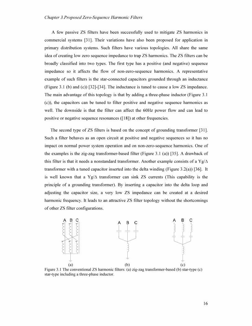
A few passive ZS filters have been successfully used to mitigate ZS harmonics in
commercial systems [31]. Their variations have also been proposed for application in
primary distribution systems. Such filters have various topologies. All share the same
idea of creating low zero sequence impedance to trap ZS harmonics. The ZS filters can be
broadly classified into two types. The first type has a positive (and negative) sequence
impedance so it affects the flow of non-zero-sequence harmonics. A representative
example of such filters is the star-connected capacitors grounded through an inductance
(Figure 3.1 (b) and (c)) [32]- [34]. The inductance is tuned to cause a low ZS impedance.
The main advantage of this topology is that by adding a three-phase inductor (Figure 3.1
(c)), the capacitors can be tuned to filter positive and negative sequence harmonics as
well. The downside is that the filter can affect the 60Hz power flow and can lead to
positive or negative sequence resonances ( [18]) at other frequencies.
The second type of ZS filters is based on the concept of grounding transformer [31].
Such a filter behaves as an open circuit at positive and negative sequences so it has no
impact on normal power system operation and on non-zero-sequence harmonics. One of
the examples is the zig-zag transformer-based filter (Figure 3.1 (a)) [35]. A drawback of
this filter is that it needs a nonstandard transformer. Another example consists of a Yg/∆
transformer with a tuned capacitor inserted into the delta winding (Figure 3.2(a)) [36]. It
is well known that a Yg/∆ transformer can sink ZS currents (This capability is the
principle of a grounding transformer). By inserting a capacitor into the delta loop and
adjusting the capacitor size, a very low ZS impedance can be created at a desired
harmonic frequency. It leads to an attractive ZS filter topology without the shortcomings
of other ZS filter configurations.
(a) (b) (c)
Figure 3.1 The conventional ZS harmonic filters: (a) zig-zag transformer-based (b) star-type (c)
star-type including a three-phase inductor.

Chapter 3.Proposed Zero-Sequence Harmonic Filters
17
3.2 Proposed Double-Tuned ZS Filter
Built on the work of [31] and [36], this chapter presents a novel double-tuned,
transformer-based ZS filter. Since the filter can trap two ZS harmonics, it is very
attractive to solve problems that involve two dominant harmonics, such as the telephone
interference problem. Telephone interference is normally caused by the ZS 9th and 15th
harmonics (For more information about telephone interference, refer to section 3.4.2). In
fact, the proposed filter is conceived originally as a tool to solve telephone interference
problems. The use of only one single-tuned ZS filter will have difficulty in solving these
problems.
The proposed ZS harmonic filter is developed by expanding the conventional ZS
filters consisting of Yg/∆ transformers. This new double-tuned topology is depicted in
Figure 3.2 (b).
(a) (b)
Figure 3.2 The transformer-based ZS filter topologies: (a) conventional single-tuned version (b)
proposed double-tuned version.
In Figure 3.3, a sample ZS impedance frequency scan of the proposed filter tuned to
both the 9th and 15th harmonic frequencies is shown and compared with the single-tuned
version.
1 3 5 7 9 11 13 15 17 19 21 23 25 27 2910
100
10000
Frequency(pu)
Zer
o S
eq
uen
ce
imped
ance (
Ω)
The Single Tuned
The Double Tuned
Figure 3.3 Zero-sequence frequency scan of the designed filters

Chapter 3.Proposed Zero-Sequence Harmonic Filters
18
The theoretical principles of the proposed filter can be understood by studying this
filter’s equivalent ZS circuit. Figure 3.4 (a) shows a single-tuned ZS filter, illustrating
how to derive its equivalent ZS circuit. A ZS voltage (V0) is applied to the filter. The
Kirchhoff's Voltage Law (KVL) implies that, in the secondary side of the transformer,
0 0
0 0
0
13 3( )
T T
I IaV R jh L
a jh C aω
ω
= + + , ( 3.1)
where a is the transformer secondary to primary winding ratio, ω0 is the power
fundamental frequency(rad/sec), h is the harmonic order, and RT and LT are transformer
winding resistance (Ω) and leakage inductance (H), transferred to the secondary side,
respectively. From ( 3.1), the equivalent ZS impedance of the filter at harmonic order h
can be calculated:
0
0 02
00
1 1( ) ( )
3f T T
VZ h R j h L
a h CIω
ω
= = + − . ( 3.2)
Next, the equivalent ZS circuit of the filter can be established as depicted in Figure 3.4
(b). Equation ( 3.2) shows that the capacitor can be tuned to make the reactance part of the
filter impedance zero for a specific harmonic. In this case, the filter impedance at the
tuned harmonic would be only the transformer winding resistance value transferred to the
primary side. For example, to tune the filter to the 9th harmonic (by making the reactance
part of ( 3.2) zero), the required capacitor size can be calculated as follows:
2 2 2
0 0
1 1
3 243T T
Ch L Lω ω
= = . ( 3.3)
0V
0I
0aV
0I
a0
I
0I
0V
0V
0aV
0aV
(a) (b) (c)
Figure 3.4 (a) The ZS filter (b) The equivalent ZS circuit of single-tuned ZS Filter (c) The
equivalent ZS circuit of the double-tuned ZS Filter
With a similar procedure, the equivalent ZS circuit of the proposed double-tuned ZS
filter can be derived as shown in Figure 3.4 (c). The obtained equivalent ZS circuit is

Chapter 3.Proposed Zero-Sequence Harmonic Filters
19
very similar to the conventional double-tuned filters shown in Figure 3.5(b). Therefore,
the proper component sizes of the proposed double-tuned ZS filter can be also derived by
using a similar mathematical approach as follows [1]:
According to [1], the equivalent impedances of two parallel conventional single-tuned
filters (Figure 3.5 (a)) close to their tuned harmonic frequencies are almost the same as
those of a conventional double-tuned configuration (shown in Figure 3.5 (b)), subject to
the following relationships among their component parameters:
2
2
2
2
,
( )( )
( )
( )
( ) ( )
a bx a b x
a b
a b a b a by
a a b b
a a b by
a b a b
L LC C C L
L L
C C C C L LC
L C L C
LC L CL
C C L L
= + =
+ + +
=−
− =
+ +
( 3.4)
To establish the mathematical expressions for a double-tuned ZS filter tuned to the
harmonic orders hi and hj, two single-tuned ZS filters separately tuned to hi and hj can be
considered with the respective capacitor sizes of Ci and Cj , as in ( 3.5):
2 2 2 2
0 0
1 1,
3 3i j
i T j T
C Ch L h Lω ω
= = . ( 3.5)
The two parallel single-tuned filters (shown in Figure 3.5 (a)) are supposed to
represent the equivalents of the two single-tuned ZS filters; therefore, their inductors and
capacitor sizes are subject to the following relationships:
2 2
2 2
a i b j
,
C =3a C , C =3a C
T T
a b
L LL L
a a
= =
( 3.6)
(a) (b)
Figure 3.5 (a) Two paralleled conventional single-tuned filters (b) The conventional double-tuned
filter.

Chapter 3.Proposed Zero-Sequence Harmonic Filters
20
The component sizes of the double-tuned ZS filter can be obtained by using the
equations set of ( 3.4). The only challenging issue involves Lx , which is the transformer
leakage inductance. By comparing Figure 3.4 (c) and Figure 3.5(b), Lx is observed to be
equal to LT/a2 , on the other hand, according to ( 3.4), Lx has to be
(3.6)
22
a b T
x
a b
L L LL
L L a= =
+
( 3.7)
To overcome this problem, one can divide the impedance value of every component
of the double-tuned filter by two (i.e., divide/multiply the inductance/capacitance values
by two) in order to satisfy ( 3.7) while keeping the tuned harmonic frequencies of the filter
unchanged:
2 2
1 2
2
2 2
2(3 ), 2(3 )
1 1( ), ( )
2 2 3
x y
Tx y
C a C C a C
L LL L
a a
= =
= =
. ( 3.8)
Finally, combining equations ( 3.4), ( 3.6) and ( 3.8) leads to the final expressions for
deriving the component sizes of the proposed ZS double-tuned filter as follows,
1
2
i jC C
C+
= , ( 3.9)
2 2
2 ( )
( )
i j i j
i j
C C C CC
C C
+=
−, ( 3.10)
2
2 2
3 ( )
( )
T i j
i j
L C CL
C C
−=
+, ( 3.11)
where Ci and Cj are the capacitors tuned for the single-tuned ZS filters as defined in ( 3.5).
For both the double-tuned and single-tuned ZS filters, the filter equivalent ZS impedance
at the tuned frequencies is equal to transformer winding resistance referred to the primary
side. For the filter to be effective, this resistance must be smaller than the system
impedance.
3.3 Filter Construction & Design
Creating a low-resistance transformer does not involve any technical difficulties.
However, constructing a ZS filter by using a specially designed MV transformer is highly
uneconomical and must be avoided. A distribution utility company often has thousands of
service transformers. If such transformers can be used, the filter cost can be reduced

Chapter 3.Proposed Zero-Sequence Harmonic Filters
21
significantly. Furthermore, the LC components of the filter can be treated as the “loads”
of the transformer. Installing a filter then becomes the same as adding a new “customer”
to the system. To this end, the impedance characteristics of common service transformers
have been investigated. The results show that one three-phase or three single-phase
service transformers in the range of total 100kVA to 450kVA are sufficient to create an
effective ZS filter. The secondary side voltage can be 480V or 208V. As a result, the
proposed filter becomes a very attractive method for mitigating ZS harmonics.
The transformer size can be determined by comparing the system impedance with the
transformer resistance (see Section 3.4.4). A more accurate size determination may be
accomplished through Harmonic Load Flow (HLF) studies. Once the transformer size is
selected, specification of the other filter components can be derived by using equations
( 3.3) or ( 3.5), ( 3.9)-( 3.11) for the single tuned or the double-tuned versions, respectively.
Another factor to consider is that the transformer must not be overloaded by the
harmonics it traps. This consideration creates the need to determine the loading
conditions of the filter transformer. For this purpose, an index called the TLL
(Transformer Loading Level) is developed. The details are presented in the Appendix B.
If the index exceeds 1pu (indicating that the transformer is overloaded), a larger
transformer must be utilized. The calculation of TLL becomes a part of the filter design
process.
For assessing the loading of the capacitors, guidelines are already provided in the
standards [37]. For the capacitors inside a ZS filter, however, their capacitance must not
be changed in case of overloading (because the capacitances are strictly determined by
the transformer specifications as in ( 3.9)-( 3.10)). Therefore, to alleviate the loading of
such capacitors, one has to increase their rated voltage and kvar without altering their
capacitance (uF).
Based on the above considerations, the overall design procedure of the proposed ZS
filters is presented in Figure 3.6. The filter placement procedure is dependent on the type
of the problem to be solved. In Section 3.4.3, the filter locating issues specific to a
telephone interference problem will be discussed.

Chapter 3.Proposed Zero-Sequence Harmonic Filters
22
Figure 3.6 The flowchart of design procedure for the proposed ZS filters
3.4 Application Example
The proposed ZS filter and its design procedure were tested by solving a telephone
interference problem faced by an actual system. Telephone interference is probably the
most common issue caused by ZS harmonics. Subsection 3.4.1 presents some information
regarding the studied telephone interference problem. In subsection 3.4.2, the telephone
interference problem is quantified and a mitigation objective is established. The number
of required filters and their placement issues are discussed in subsection 3.4.3. Next, in
subsection 3.4.4, the ZS filters are designed based on the proposed procedure. Different
filter case studies are also performed and discussed in this section. At the end, subsection
3.4.5 evaluates loading of the designed filters based on the proposed methodology.

Chapter 3.Proposed Zero-Sequence Harmonic Filters
23
3.4.1 Problem Description
The studied telephone interference problem is associated with the actual feeder
introduced in Chapter 2. As shown in Figure 3.7, a telephone-line is experiencing severe
disturbing noises induced by the feeder’s adjacent overhead sections. The sections in
parallel with the overhead power lines are shown by the dashed lines in Figure 3.7 (The
effect of the underground sections in noise induction is negligible since the neutral
conductor is very close to the phase conductors in an underground cable and also carries
the whole returning current, canceling out the overall generated electromagnetic field).
The ZS filters will be examined by the developed simulation platform described in
Chapter 2. Additionally, since the neutral wires are also included by the multi-phase
models, the telephone lines can be also added to the model for the interference level
assessment. For this case, two sample parallel conductors are also included in the system
model for representing the involved telephone line sections (dashed lines in Figure 3.7).
Figure 3.7 The schematic view of the studied distribution feeder
3.4.2 Telephone Interference Mitigation Objective
The ZS component of the harmonic currents in an overhead power-line is the
dominant source of the noise induction on the adjacent telephone lines [26], [38]. Most of
the ZS component of a harmonic current is dominated by the triplen harmonic orders
such as 3rd, 9th, 15th. As well, for the telephone interference, the “C-message” factors
determine the contribution of each harmonic frequency to the disturbing noise [26], [38].

Chapter 3.Proposed Zero-Sequence Harmonic Filters
24
The C-message factors, which are presented in [38] (shown in Table 3.1) are derived on
the basis of the sensitivity of the human ear and the vulnerability of the communication
circuits to different noise frequencies.
Table 3.1 C-message weighting factors for different harmonic frequencies
Harmonic order 1 3 5 7 9 11 13 15
C-message
weighting factor 0.001 0.033 0.150 0.309 0.488 0.684 0.861 0.966
The factor is very small for the 3rd harmonic compared to that for the higher-order
ones. Since the magnitude of harmonic orders higher than the 15th in residential
distribution system is negligible, the 9th and 15th ZS harmonic orders can be identified as
the main contributors to a telephone interference problem. Therefore, the proposed
double-tuned filter will be tuned to the 9th and 15th harmonic frequencies.
As recommended by [38], the actual interference level can be quantified by
multiplying the induced voltage of each harmonic frequency on the communication line
by its corresponding C-message factor. Therefore, an index called the ‘C-Message
Weighted Voltage’ (CMWV) can be defined as below:
h h hCMWV w V= , ( 3.12)
where Vh and wh are the induced voltage of hth harmonic frequency on the telephone line
and its corresponding C-message weighting factor, respectively. Next, the total value of
the CMWV determined by ( 3.12) can exhibit the total interference level:
2
1,3,...
total h
h
CMWV CMWV
=
= ∑ . ( 3.13)
The above index was adopted for this thesis to assess the effectiveness of the
mitigation techniques for the telephone interference problem. The mitigation objective
used to find the final filter design was set to be a 75% decrease of the total interference
level (CMWVtotal).
3.4.3 Filter Location
In order to effectively mitigate a telephone interference problem, the installation of
harmonic filters must eliminate the troublesome ZS harmonic currents in the power-line

Chapter 3.Proposed Zero-Sequence Harmonic Filters
25
sections causing the disturbance. This section investigates the required number of filters
and their appropriate placement in the studied feeder (shown in Figure 3.7).
During the normal system condition, most load-generated harmonic currents flow to
the substation due to the low supply system impedance. The ideal location for installing
the filter to mitigate the telephone interference problem is at the downstream side of the
telephone line such as location ‘F1’ shown in Figure 3.7. The filter is expected to sink the
harmonics produced by the downstream loads. Thus, these harmonics will not travel
upstream and interfere with the telephone line upstream. However, an important issue
must be addressed here: Will the filter also attract the harmonics from the upstream loads?
If the filter does so, it may not be able to reduce the telephone interference level. HLF
simulation results can determine whether this issue will be a problem or not. If a problem
is caused in the mitigation, then two filters will be required, and the second one will need
to be installed at the location between the telephone line and the upstream loads (labelled
by F2 in Figure 3.7).
3.4.4 Filter Design Results
For selecting the transformer size, some of the typical sizes of the three-phase
transformers used by the utility company in their 25kV voltage level distribution systems
are listed in Table 3.2. The ZS impedance of the filter at the tuned harmonics obtained by
each of the transformer sizes is also provided in the last column.
Table 3.2 The (ZS) filter impedance obtained by different sizes of transformers
Transformer
S (kVA) Vlow (V)a
Rpu (%) Zpu (%) Zfilter(Ω)
9750 208 0.93 5.3 0.59
7500 208 0.93 5.3 0.77
2500 600 0.52 5.75 1.29
1500 480 0.72 5.9 2.99
1000 600 0.73 4.7 4.53
500 600 0.84 4.36 10.39
450 480 0.89 4.28 12.29
300 208 0.88 4.3 18.18
225 600 1.03 3.88 28.56
150 208 1.19 3.32 49.51
75 208 1.13 3.22 93.96
a: The nominal line-to-line voltage of transformer (LL-rms). The primary-side voltage is 25kV
(LL-rms) for all of the listed transformers.

Chapter 3.Proposed Zero-Sequence Harmonic Filters
26
On the other hand, the system model is also used to estimate the system equivalent ZS
impedance at the 9th and 15th harmonic frequencies at the proposed filter location (F1 in
Figure 3.7). The obtained minimum values during the day are 56.84Ω and 41.6Ω for the
9th and 15th harmonic orders, respectively. Because of these values, the transformer size
of 225 kVA is adopted as the minimum transformer size to be used in the ZS filter design
procedure. As Table 3.2 shows, this transformer size provides a 28.56 Ω filter impedance,
which is smaller than the minimum value of the system impedance at 9th and 15th
harmonics.
The introduced iterative process (Figure 3.6) was employed to determine the final
filter design. Table 3.3 presents the component sizes of the designed filter package. Two
filters at both the F1 and F2 locations (in Figure 3.7) were required to fulfill the
mitigation objective of a 75% decrease in the interference level. In addition, a single-
tuned version of the ZS filter with the same transformer size (450kVA) and tuned to the
9th harmonic was also designed and modeled in the simulations for a comparative study.
As Table 3.3 shows, the capacitor sizes required for the double-tuned filter were larger
than those of the single-tuned one, but the values are still practical and not too large if
compared with those of the conventional filter designs. Figure 3.3 shows the ZS
impedance of the designed filter configurations for different harmonic frequencies.
Table 3.3 Designed Components Size for the Single and Double-Tuned Filters
Transformer Size The Single-Tuned The Double-Tuned
C C1 C2 L2 450 kVA 44.20 kvar
a 30.05 kvar 105.66 kvar 37.80 µH
a: The kvar value is calculated by assuming the transformer secondary-side voltage (480V) as the
rating value of capacitor.
In order to establish a sound understanding of the discussed ZS filters performance,
the HLF simulation results for the following cases are also presented and discussed in this
section.
• Case I: normal system condition before installing any filter.
• Case II: one single-tuned version of the designed ZS filter (with 450kVA
transformer) is installed in location F1.
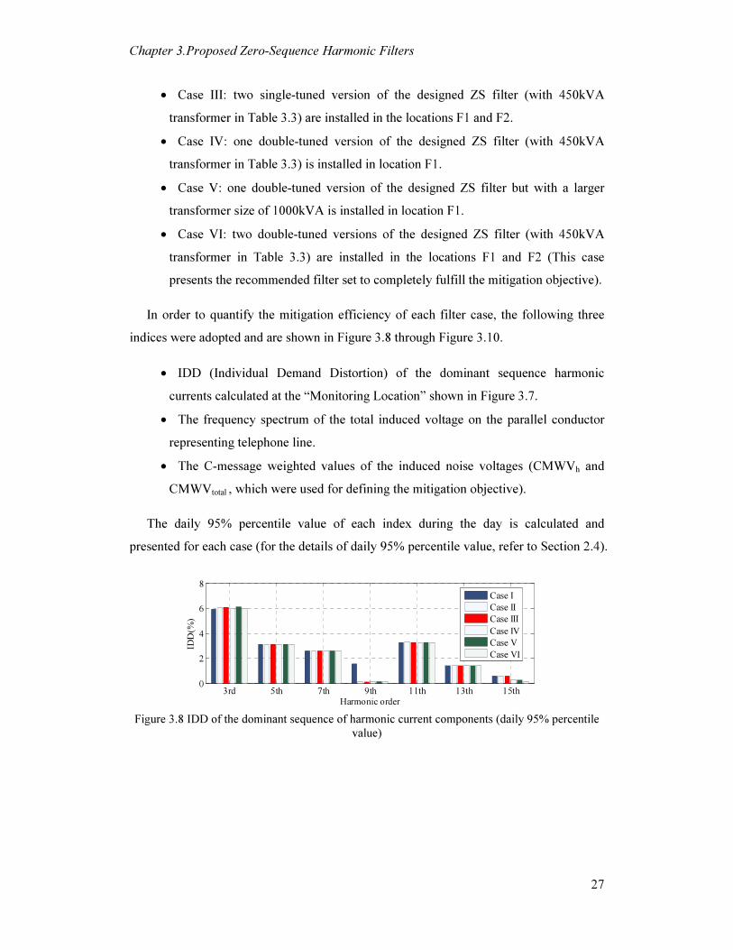
Chapter 3.Proposed Zero-Sequence Harmonic Filters
27
• Case III: two single-tuned version of the designed ZS filter (with 450kVA
transformer in Table 3.3) are installed in the locations F1 and F2.
• Case IV: one double-tuned version of the designed ZS filter (with 450kVA
transformer in Table 3.3) is installed in location F1.
• Case V: one double-tuned version of the designed ZS filter but with a larger
transformer size of 1000kVA is installed in location F1.
• Case VI: two double-tuned versions of the designed ZS filter (with 450kVA
transformer in Table 3.3) are installed in the locations F1 and F2 (This case
presents the recommended filter set to completely fulfill the mitigation objective).
In order to quantify the mitigation efficiency of each filter case, the following three
indices were adopted and are shown in Figure 3.8 through Figure 3.10.
• IDD (Individual Demand Distortion) of the dominant sequence harmonic
currents calculated at the “Monitoring Location” shown in Figure 3.7.
• The frequency spectrum of the total induced voltage on the parallel conductor
representing telephone line.
• The C-message weighted values of the induced noise voltages (CMWVh and
CMWVtotal , which were used for defining the mitigation objective).
The daily 95% percentile value of each index during the day is calculated and
presented for each case (for the details of daily 95% percentile value, refer to Section 2.4).
3rd 5th 7th 9th 11th 13th 15th0
2
4
6
8
IDD(%
)
Harmonic order
Case I
Case II
Case III
Case IV
Case V
Case VI
Figure 3.8 IDD of the dominant sequence of harmonic current components (daily 95% percentile
value)

Chapter 3.Proposed Zero-Sequence Harmonic Filters
28
1st 3rd 5th 7th 9th 11th 13th 15th Total rms0
50
100
Indu
ced V
olt
age(V
)
Harmonic order
Case I
Case II
Case III
Case IV
Case V
Case VI
Figure 3.9 The harmonic spectrum of induced voltage on the parallel conductor (daily 95%
percentile value)
1st 3rd 5th 7th 9th 11th 13th 15th Total0
20
40
60
C-m
essa
ge w
eig
hte
d V
olt
age(
V)
Harmonic order
Case I
Case II
Case III
Case IV
Case V
Case VI
Figure 3.10 C-message weighted voltage components induced on the parallel conductor (daily
95% percentile value)
The following are the key observations from the simulation results:
• The results imply that the final designed filter set (case VI) effectively removed
both the 9th and 15th harmonic components in either the power-line current (Figure
3.8) or the induced voltage on the parallel conductor (Figure 3.9). By lowering the
total CMWV from 56.5V to 12V, the goal of a 75% decrease in interference level
was achieved (Figure 3.10).
• The double-tuned ZS filters were found to be effective in mitigating both the 9th
and 15th harmonics. Although the single-tuned versions could suppress the 9th
harmonic, they were unable to mitigate the 15th harmonic. The 15th harmonic
component was observed to increase in the single-tuned filter cases (II & III) and
to cause a mitigation failure (See Figure 3.9 and Figure 3.10). This phenomenon
is likely due to a parallel resonance between the filter and the system at the 15th
harmonic frequency. At this harmonic frequency, the filter is inductive and the
system is capacitive because of the shunt capacitance of the underground cables.
Such observations once again confirm the need to use the proposed double-tuned
ZS filter to mitigate a telephone interference problem.

Chapter 3.Proposed Zero-Sequence Harmonic Filters
29
• One single filter at location F1 was observed to be sufficient for effectively
mitigating the 9th harmonic. However, the single location filter scenarios (cases
IV & V) could not decrease the 15th harmonic by more than 40%. Specifically,
case V even with a considerably larger transformer (1000kVA), did not lead to a
further reduction of the 15th harmonic. Nonetheless, a single designed filter (case
IV) mitigated almost 48% of the interference level, as shown in Figure 3.10.
However, to achieve the mitigation objective of a 75% decrease in the noise level,
two of the designed double-tuned filter packages were required at both locations
F1 and F2.
• As we expected, Figure 3.8 shows that, the ZS filters had no effect on the
positive/negative sequence harmonic components. For all the filter scenarios, the
non-triplen harmonic values were not changed from the case without any filter.
3.4.5 Filter Loading Assessment Results
The procedure described in the Appendix B was employed to evaluate the loading of the
transformer inside the designed double-tuned ZS filters. The harmonic currents flowing
inside the transformers were obtained from the simulations and are shown in Figure 3.11,
which shows that the 9th and 15th harmonic currents, which the filters were tuned to, were
the dominant components.
1 5 9 13 17 210
1
2
3
4
Time(hour)
Har
mon
ic C
urr
en
t(A
)
1 5 9 13 17 210
0.5
1
1.5
2
Time(hour)
Har
mon
ic C
urr
en
t(A
)
9th
15th
9th
15th
(a) (b)
Figure 3.11 Daily profile of harmonic currents flowing inside the transformer (primary side) of the
designed ZS filters (a) at location ‘F1’ (b) at location ‘F2’.
An analysis was conducted for both dry-type and liquid-filled transformers. As given
in Table 3.4, conservative values for PEC-R(pu) and POSL-R(pu) were adopted based on the
transformer size (450kVA) and the data presented in Table B.1. POSL-R(pu) was also

Chapter 3.Proposed Zero-Sequence Harmonic Filters
30
calculated by using equation (B.8) in the Appendix. The TLL index was calculated for
both filters’ transformers and is presented in Figure 3.12.
1 5 9 13 17 210
0.5
1
Time(hour)Tra
nsf
orm
er
Load
ing
Lev
el(
pu
)
Dry type Liquid-filled type
1 5 9 13 17 210
0.5
1
Time(hour)
(a) (b)
Figure 3.12 Estimated daily profile of the transformer loading level (TLL) for the designed ZS
filters (a) at location ‘F1’ (b) at location ‘F2’
The results illustrate that the transformers loading level was under the eligible
maximum (1pu) for the whole day; therefore, the designed filters could operate safely
without overloading their transformers.
Table 3.4 The adopted values of PEC-R and POSL-R for the loading assessment
Transformer type Dry type Liquid-filled type
PEC-R(pu) 0.08 0.05
POSL-R(pu) 0.04 0.1
3.5 Conclusions
This chapter presented a novel and effective filter to mitigate ZS harmonics in the power
systems. The design and construction issues of the filters are fully investigated. The main
findings and contributions of this work can be summarized as follows.
• The proposed filter can trap two harmonics simultaneously. It becomes a very
attractive method to mitigate telephone interference problems.
• The filter can be constructed using regular service transformers and low voltage
LC components. As a result, it is a very cost-effective filter. Installing a filter is as
sample as adding a customer to the distribution system.
• A practical design procedure has been developed for the filter. This chapter also
presented a method for loading assessment of the filter transformer.
• The proposed filter package and its design method have been tested through
computer simulation studies. The results have shown that the filter is quite

Chapter 3.Proposed Zero-Sequence Harmonic Filters
31
effective to trap zero sequence harmonics and is an attractive solution to the
telephone interference problem.

Chapter 4. Design of Medium-Voltage Passive Harmonic Filters
32
Chapter 4
Design of Medium-Voltage Passive Harmonic Filters
The shunt connected passive harmonic filters are a popular choice for the medium- and
high-voltage applications in power systems [3], [8]- [11], [14]. This chapter discusses the
option of installing Medium-Voltage (MV) filters to achieve a system-wide harmonic
mitigation in residential distribution power systems. The proposed ZS filters in Chapter 3
are also included to develop an effective MV filter package. An iterative design
procedure is introduced. It helps to simplify addressing the complex problem of
designing such filters to mitigate distributed harmonic sources.
The chapter is organized as follows. Section 4.1 describes the adopted passive MV
filter topologies. The key considerations required for designing the MV passive filters are
reviewed in section 4.2. A general and practical design procedure is proposed in section
4.3. This procedure serves as a practical guideline for designing MV passive filters to
mitigate the harmonics of a residential feeder. The proposed method is employed in
section 4.4 to design MV filters for both the studied feeders in order to accomplish the
mitigation goals defined in this thesis. The final design specifications for the feeders are
tabulated in section 4.5. Section 4.6 presents a summary of the contents of this chapter.
4.1 MV Passive Harmonic Filter Package
One of the first important steps in designing a passive harmonic filter is to select the
proper topology. Most of the filter topology studies such as [8], [12] have focused on the
industrial harmonic sources. The results of these investigations as well as the common
industry practice recommend the conventional single-tuned filters as the preferred
topologies based on the economic and design issues. However, as discussed before, there
is also considerable amount of ZS harmonics such as 3rd, 9th and 15th in a residential
distribution feeder. Therefore, the proposed double-tuned ZS filter introduced in Chapter
3 is also included in the suggested MV filter package to mitigate 3rd and 9th harmonics as
well. Using the ZS filter instead of the single-tuned filters for eliminating the ZS
harmonics has the following advantages:

Chapter 4. Design of Medium-Voltage Passive Harmonic Filters
33
1) The ZS filter will not adversely affect the reactive power profile and other non-ZS
harmonics of the system.
2) Compared to the alternative choice of two single-tuned filters tuned to the ZS
harmonics, the double-tuned ZS filter can be a much simpler and less expensive option
(The economic analysis in the consequent chapter will demonstrate this fact).
Figure 4.1 shows the selected MV filter package for this chapter studies.
Figure 4.1 The MV level passive filter package consisting of a double-tuned ZS filter and the
conventional single-tuned filter branches.
4.2 Design Considerations
Several constraints and issues have to be considered when designing a passive harmonic
filter. This section discusses the key design issues thereby developing a general design
guideline.
4.2.1 System Reactive Power Profile
Traditionally, the capacitors of harmonic filters were sized according to the reactive
power requirements of the system [8], [12]. However, the distribution feeders serving
residential loads generally do not require a planned reactive power compensation. Such
systems usually include several underground cable sections so that their shunt
capacitances collectively lead to a considerable source of reactive power.
For example, Figure 4.2 and Figure 4.3 show the estimated daily profile of
real/reactive power associated with the real and ideal feeders monitored in substation
obtained from simulation results. The reactive power consumption of both feeders is
negligible and it is even negative in some hours for the actual feeder (Figure 4.2) which is
due to the shunt capacitance of its underground cables.
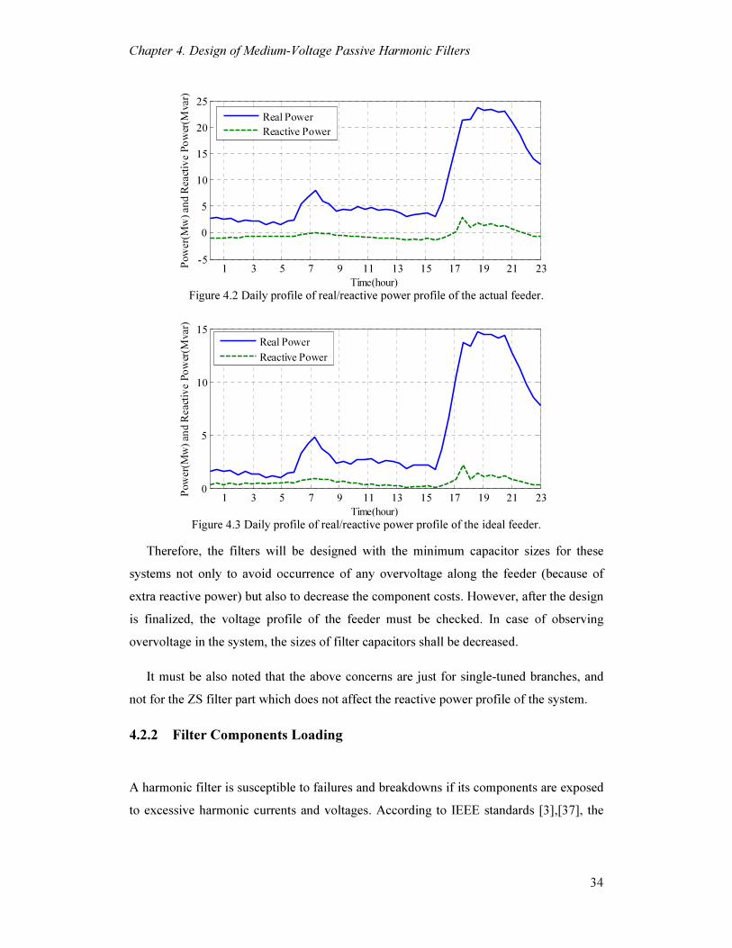
Chapter 4. Design of Medium-Voltage Passive Harmonic Filters
34
1 3 5 7 9 11 13 15 17 19 21 23-5
0
5
10
15
20
25
Time(hour)
Pow
er(
Mw
) an
d R
eact
ive P
ow
er(M
var)
Real Power
Reactive Power
Figure 4.2 Daily profile of real/reactive power profile of the actual feeder.
1 3 5 7 9 11 13 15 17 19 21 230
5
10
15
Time(hour)
Pow
er(
Mw
) an
d R
eact
ive P
ow
er(M
var)
Real Power
Reactive Power
Figure 4.3 Daily profile of real/reactive power profile of the ideal feeder.
Therefore, the filters will be designed with the minimum capacitor sizes for these
systems not only to avoid occurrence of any overvoltage along the feeder (because of
extra reactive power) but also to decrease the component costs. However, after the design
is finalized, the voltage profile of the feeder must be checked. In case of observing
overvoltage in the system, the sizes of filter capacitors shall be decreased.
It must be also noted that the above concerns are just for single-tuned branches, and
not for the ZS filter part which does not affect the reactive power profile of the system.
4.2.2 Filter Components Loading
A harmonic filter is susceptible to failures and breakdowns if its components are exposed
to excessive harmonic currents and voltages. According to IEEE standards [3], [37], the

Chapter 4. Design of Medium-Voltage Passive Harmonic Filters
35
voltage and current waveform during operation of filter capacitors are required not to
exceed the following limits.
a) 110% of rated rms voltage.
b) 120% of rated peak voltage (i.e. rated rms voltage multiplied by square root of two).
c) 135% of nominal rms current based on rated kvar and voltage.
d) 135% of rated kvar.
During the design procedure, loading condition of all the filter capacitors have to be
analyzed according to the above standard limits. If the operation current and voltage of a
capacitor is observed to exceed the limits in simulations, its size must be increased.
However, for the capacitors inside the ZS filter, both of their kvar and rated voltage have
to be increased to avoid changing their capacitance.
The loading level of the transformer inside the ZS filter can be also assessed by the
procedure developed in Chapter 3. Again, if its loading analysis illustrates an overloading
condition, a larger size of transformer must be chosen.
4.2.3 Filter Placement
In the traditional harmonic filter applications, filters have been installed at the PCC of the
large and known harmonic-generating load and therefore placement has not been a major
filter design issue. However, in the residential distribution systems harmonic sources are
not concentrated in single points and can be dispersed all along the feeder. As discussed
in Chapter 1, several algorithms and strategies have been developed for allocation and
placement of passive filters in a distribution system [15]- [17]. Such algorithms are too
complex and need several computational efforts. Besides, since most of them are
developed on the basis of oversimplified harmonic models, they can not be employed for
the simulation platform of this thesis. Therefore, this thesis tackles such complex problem
of filter placement for distributed sources with a simplified and practical iterative
approach as described below.
1) The possible locations for the passive filters are identified in each feeder.
2) The filter design procedure starts with a minimum size package.
3) The filter package performance is then assessed by running the HLF simulations for
the different locations. If the mitigation objective is achieved by installing the filter in

Chapter 4. Design of Medium-Voltage Passive Harmonic Filters
36
one of the locations, then the filter design is finalized and the location with the highest
elimination of harmonics is chosen. However, if none of the locations can bring the
expected mitigation efficiency, the filter package design will be improved and the whole
process will be repeated for the new package again.
4) In case one filter package fails to obtain the mitigation goals, the design procedure
can be continued with installing two harmonic filters in two locations.
4.3 Overall Design Procedure
The overall passive harmonic filter design procedure is established in this section based
on the discussions in section 4.2. Figure 4.4 illustrates an overall view of the proposed
methodology in which the placement and loading assessment considerations are
combined into the proposed iterative procedure.
Figure 4.4 The proposed iterative design procedure in a quick view.
Figure 4.5 shows every details of the design process where the filter improvement
block in Figure 4.4 is also expanded. As shown in the flowchart, the whole procedure can
be explained as below:
• The first step in improving the filter package is increasing capacitor size of
single-tuned branches. The inductors are also sized accordingly (For further
details of designing single-tuned branches, refer to Appendix C.1). The

Chapter 4. Design of Medium-Voltage Passive Harmonic Filters
37
capacitor size can be increased up to their maximum limit (which is chosen by
the designer in the beginning of process).
• If the capacitors sizes reach their maximum limit and filter package still
needs to be improved, the second step will be taken that is to enlarge the ZS
filter transformer. Then, the other components of the ZS filter can be designed
accordingly based on the guidelines developed in Chapter 3.
• If the larger transformer sizes of ZS filter also fail to achieve the essential
filtering improvements, the designer can consider the addition of a new single-
tuned branch to the filter package. However, in the proposed design procedure,
maximum number of single-tuned branches is considered to be three.
• In case a filter package even including three single-tuned branches beside the
ZS filter is still unable to gain the mitigation objective, the designer has to
choose the option of installing two filter packages in two different locations of
the feeder.
• Setting the harmonic mitigation objective was fully discussed in Chapter 2.
In summary, the goal is to decrease both the average voltage THD over the
feeder and harmonic current TDD in substation by 75% (the daily 95%
percentile values are considered).

Chapter 4. Design of Medium-Voltage Passive Harmonic Filters
38
Figure 4.5 Detailed flowchart of the proposed design procedure for the MV passive filter.

Chapter 4. Design of Medium-Voltage Passive Harmonic Filters
39
4.4 Iterative Design Results
The proposed procedure is employed to design the passive MV filters for both of the real
and ideal feeder. The iterative route taken to obtain the final proper design for each of the
systems is presented in this section.
Table 4.1 lists the different sizes of transformers used for design of ZS filter. The
standard capacitor sizes of 150,300,450,600,900 and 1200 kvar are also adopted in this
design [37].
Table 4.1 List of transformers used for the filter design.
Transformer
S
(kVA)
Vlow
(V)a
Rpu
(%)
Zpu
(%) Zfilter(Ω)
300 208 0.88 4.3 18.18
500 600 0.84 4.36 10.39
1000 600 0.73 4.7 4.53
2500 600 0.52 5.75 1.29
a: The nominal secondary-side voltage of transformer (LL-rms).
The primary-side voltage is 25kV for all of the listed transformers.
Regarding the filter location(s), two potential locations are chosen for the actual
feeder labeled as ‘MV I’ and ‘MV II’ in Figure 4.12. For the ideal feeder, four possible
locations are selected along the feeder with the distances of 3, 7, 10 and 13km from the
substation, respectively.
For selection of the tuning frequencies, the harmonic distortion spectrum of the
feeders shown in Figure 4.6 and Figure 4.7 must be considered. For both of the feeders,
the ZS filter will be tuned to 3rd and 9th which are the dominant ZS components. Among
the other harmonic orders, 5th and 11th are the dominant ones so that they are chosen as
the tuning frequencies for the first two single-tuned branches. The next branch, if
necessary, will be tuned to 7th (for the actual feeder, one branch will be tuned to 13th
rather than 11th due to its special system impedance. More details will be provided in
section 4.4.2).

Chapter 4. Design of Medium-Voltage Passive Harmonic Filters
40
3rd 5th 7th 9th 11th 13th 15th THD
0
2
4
6
8
Volt
age I
HD
(%)
Harmonic order
Ideal Feeder
Actual feeder
Figure 4.6. Votage IHD of both feeders average over feeder before filter installation (daily 95%
percentile value).
3rd 5th 7th 9th 11th 13th 15th TDD
0
2
4
6
8
Curr
en
t ID
D(%
)
Harmonic order
Ideal Feeder
Actual feeder
Figure 4.7 Current IDD of both feeders at the substation before filter installation (daily 95%
percentile value).
Sections 4.4.1 and 4.4.2 present the design procedure and results for the ideal and
actual feeders, respectively.
4.4.1 For Ideal Feeder
Table 4.2 lists the cases which are iteratively generated to find the final MV passive filter
design for the ideal feeder. As seen in the table, each case has been examined in all the
four locations. The results show that two single-tuned branches beside the ZS filter can
not be sufficient to achieve the mitigation objective and a third branch is also essential.
For example, in cases no. 17 to 19, although maximum size of transformers and
capacitors are used, the percentage decrease of voltage THD is still less than the defined
goal of 75%.
By addition of a 7th single-tuned branch, the filter performance is improved. Finally,
for case no. 50 (which is highlighted in the table) the aimed decrease in THD and TDD is
obtained. The filter components are also not overloaded in this case. The filter location of
this final design is 7km from substation, which is almost in the middle of the feeder.
Chapter 4. Design of Medium-Voltage Passive Harmonic Filters
41
Figure 4.8 and Figure 4.9 show the system and the designed filter impedance obtained
by performing frequency scan on HLF models. Table 4.3 also gives the detail of loading
assessment of the designed filter components. All components are showing acceptable
loading level according to IEEE standards. The daily voltage profile of the feeder is also
plotted in Figure 4.10 and Figure 4.11 for the middle and the end point, respectively. As
the voltage profile shows, the designed filter not only has not caused any overvoltage
problem, but also has improved the voltage level during the peak hours. Therefore, the
performance of the designed package is also validated with regard to the system reactive
power requirements.

Chapter 4. Design of Medium-Voltage Passive Harmonic Filters
42
Table 4.2 The results of iterative filter design procedure for ideal feeder.
ZS
filter
Single tuned filter branches Filter
Location Filter effectiveness
Loading
assessment
#1 #2 #3
Case No.
Transform
er size
(kVA)
htuned Capacitor
(kvar)
htuned
Capacitor
(kvar)
htuned
Capacitor
(kvar)
Distance
from
substation
(km)
Percentage
decrease in
TDD
Percentage
decrease in
THD
Single
tuned
filters
The
ZS
filter
1 300 4.9 300 10.9 150 - - 3 36.56 26.81
2 300 4.9 300 10.9 150 - - 7 51.48 44.84
3 300 4.9 300 10.9 150 - - 10 53.99 51.11
4 300 4.9 300 10.9 150 - - 13 51.73 52.01
5 300 4.9 450 10.9 300 - - 3 37.31 29.10
6 300 4.9 450 10.9 300 - - 7 53.09 48.81
7 300 4.9 450 10.9 300 - - 10 55.80 55.74
8 300 4.9 450 10.9 300 - - 13 53.42 56.45
9 300 4.9 900 10.9 600 - - 3 37.24 31.56
10 300 4.9 900 10.9 600 - - 7 54.99 53.20
11 300 4.9 900 10.9 600 - - 10 58.33 60.71
12 300 4.9 900 10.9 600 - - 13 55.83 61.07
13 2500 4.9 600 10.9 450 - - 3 75.79 49.02
14 2500 4.9 600 10.9 450 - - 7 74.83 67.48
15 2500 4.9 600 10.9 450 - - 10 69.36 71.38
16 2500 4.9 600 10.9 450 - - 13 60.70 67.28
17 2500 4.9 1200 10.9 900 - - 3 77.63 51.94
18 2500 4.9 1200 10.9 900 - - 7 75.67 71.02
19 2500 4.9 1200 10.9 900 - - 10 70.59 73.51
20 2500 4.9 1200 10.9 900 - - 13 62.15 68.77
21 300 4.9 300 10.9 150 6.9 150 3 36.65 27.36
22 300 4.9 300 10.9 150 6.9 150 7 52.02 45.97
23 300 4.9 300 10.9 150 6.9 150 10 54.63 52.50
24 300 4.9 300 10.9 150 6.9 150 13 52.38 53.42
25 300 4.9 600 10.9 450 6.9 450 3 37.18 31.13
26 300 4.9 600 10.9 450 6.9 450 7 54.90 52.73
27 300 4.9 600 10.9 450 6.9 450 10 58.17 60.38
28 300 4.9 600 10.9 450 6.9 450 13 55.70 60.85
29 300 4.9 1200 10.9 900 6.9 900 3 35.96 33.28
30 300 4.9 1200 10.9 900 6.9 900 7 57.66 56.72
31 300 4.9 1200 10.9 900 6.9 900 10 62.14 64.57
32 300 4.9 1200 10.9 900 6.9 900 13 59.92 65.02
33 1000 4.9 600 10.9 450 6.9 450 3 73.99 47.83
34 1000 4.9 600 10.9 450 6.9 450 7 75.66 67.77
35 1000 4.9 600 10.9 450 6.9 450 10 69.56 72.19

Chapter 4. Design of Medium-Voltage Passive Harmonic Filters
43
Table 4.2 (continued).
ZS
filter
Single tuned filter branches Filter
Location Filter effectiveness
Loading
assessment
#1 #2 #3
Case No.
Transform
er size
(kVA)
htuned Capacitor
(kvar)
htuned
Capacitor
(kvar)
htuned
Capacitor
(kvar)
Distance
from
substation
(km)
Percentage
decrease in
TDD
Percentage
decrease in
THD
Single
tuned
filters
The
ZS
filter
36 1000 4.9 600 10.9 450 6.9 450 13 61.14 68.77
37 1000 4.9 1200 10.9 900 6.9 900 3 77.21 51.46
38 1000 4.9 1200 10.9 900 6.9 900 7 78.84 73.04
39 1000 4.9 1200 10.9 900 6.9 900 10 71.95 77.47
40 1000 4.9 1200 10.9 900 6.9 900 13 63.35 73.04
41 2500 4.9 450 10.9 300 6.9 300 3 80.07 48.73
42 2500 4.9 450 10.9 300 6.9 300 7 76.83 67.14
43 2500 4.9 450 10.9 300 6.9 300 10 69.45 70.98
44 2500 4.9 450 10.9 300 6.9 300 13 60.60 67.48
45 2500 4.9 900 10.9 600 6.9 600 3 86.00 52.60
46 2500 4.9 900 10.9 600 6.9 600 7 80.24 72.80
47 2500 4.9 900 10.9 600 6.9 600 10 71.73 76.67
48 2500 4.9 900 10.9 600 6.9 600 13 62.50 72.09
49 2500 4.9 1200 10.9 900 6.9 900 3 88.25 54.51
50 2500 4.9 1200 10.9 900 6.9 900 7 81.57 75.51
51 2500 4.9 1200 10.9 900 6.9 900 10 72.79 79.31
52 2500 4.9 1200 10.9 900 6.9 900 13 63.54 74.15
1 3 5 7 9 11 13 150
50
100
Frequency (pu)
Pos-
seq I
mped
ance( Ω
)
System
Filter
Figure 4.8 Positive-sequence frequency scans of the designed filter and system impedance for
ideal feeder.

Chapter 4. Design of Medium-Voltage Passive Harmonic Filters
44
1 3 5 7 9 11 13 150
50
100
Frequency (pu)
Zer
o-s
eq I
mp
ed
ance( Ω
)
System
Filter
Figure 4.9 Zero-sequence frequency scans of the designed filter and system impedance for ideal
feeder.
Table 4.3 Loading analysis of the designed filter for the ideal feeder.
Filter component Operation
value
Rated
value
Ratio of
operation to
rated value (%)
IEEE
standard
limit (%)
Is under
limit?
Peak voltage(V) 140.5 848.5 16.6 120
RMS voltage(V) 101.0 600 16.8 110
RMS current(A) 760.0 1497.2 50.8 135 C1
kvar 76.5 898.3 8.5 135
Peak voltage(V) 2.4 848.5 0.3 120
RMS voltage(V) 1.6 600 0.3 110
RMS current(A) 6.9 842.2 0.8 135
ZS filter
C2
kvar 0.0 505.3 0.0 135
Peak voltage(V) 21575.0 20365 105.9 120
RMS voltage(V) 15358.0 14400 106.7 110
RMS current(A) 30.4 27.8 109.4 135 C5th
kvar 1368.5 1200 114.0 135
Peak voltage(V) 21410.0 20365 105.1 120
RMS voltage(V) 14832.0 14400 103.0 110
RMS current(A) 21.7 20.8 104.0 135 C11th
kvar 950.2 900 105.6 135
Peak voltage(V) 21188.0 20365 104.0 120
RMS voltage(V) 15024.0 14400 104.3 110
RMS current(A) 21.9 20.8 105.0 135
Single-tuned filter branches
C7th
kvar 975.3 900 108.4 135

Chapter 4. Design of Medium-Voltage Passive Harmonic Filters
45
1 3 5 7 9 11 13 15 17 19 21 230.9
0.95
1
1.05
1.1
Time(hour)
Volt
ag
e (p
u)
No Filter
With Filter
Figure 4.10 Daily voltage profile at the middle of the ideal feeder.
1 3 5 7 9 11 13 15 17 19 21 230.9
0.95
1
1.05
1.1
Time(hour)
Volt
ag
e (p
u)
No Filter
With Filter
Figure 4.11 Daily voltage profile at the end of the ideal feeder
4.4.2 For Actual feeder
The iterative process of filter design for the actual feeder is presented in Table 4.4. The
first filter case is consisting of the ZS filter and two single-tuned branches tuned to 5th
and 13th harmonic. Differently from the designed filter for the ideal feeder, one branch is
tuned to 13th rather than 11th. The reason is that the system is observed to be capacitive in
high order harmonics (See Figure 4.13) and a filter tuned to 11th will be inductive at both
11th and 13th harmonics thereby increasing the risk of a parallel resonance between
system and the filter in such harmonic orders.
The first twelve cases in the table show that a filter with just two single-tuned
branches can not exhibit the anticipated performance. From cases number 13 to 21,
another single-tuned branch tuned to 7th harmonic is also added. These cases have been
just examined for the ‘MV II’ location since the results of first twelve cases reveal that
this location performs better rather than the ‘MV I’ (Filter locations in the actual feeder
are labeled in Figure 4.12). However, even with three single-tuned branches and selecting
the largest transformer and capacitor size, the aimed 75% decrease in current TDD is still

Chapter 4. Design of Medium-Voltage Passive Harmonic Filters
46
not achieved. Therefore, from case no. 22, two filter packages are considered to be
installed at both locations. Case no. 33 shows the final design. In this case, one of the
capacitors in the ZS filter of the ‘MV II’ location is overloaded. To address this issue, this
capacitor voltage and kvar are increased according to the proposed design guideline.
Details of loading analysis of the final designed filters are given in Table 4.5 and Table
4.6.
Figure 4.12 The MV filters locations in the actual feeder
The voltage profile of the system for both neighborhoods is also evaluated with and
without the filter in Figure 4.15 and Figure 4.16. Similarly to the ideal feeder case, the
filter is found to improve the voltage level at the peak hours. Although for the other times
of the day the filter is boosting it to higher values than 1pu, the voltage is still kept within
a 5% limit from the nominal value, which is the steady-state voltage limit commonly
adopted by distribution companies.

Chapter 4. Design of Medium-Voltage Passive Harmonic Filters
47
Table 4.4 The results of iterative filter design procedure for actual feeder.
ZS
filter Single tuned filter branches Filter(s) effectiveness
Loading
assessment
#1 #2 #3 Case No.
Transform
er
size (kVA)
htuned
Capacitor
(kvar)
htuned
Capacitor
(kvar)
htuned
Capacitor
(kvar)
Filter Location(s)
Percentage
decrease in
TDD
Percentage
decrease in
THD
Single
tuned
filters
The
ZS
filter
1 300 4.9 300 12.9 150 - - II* 52.32 51.45
2 300 4.9 300 12.9 150 - - I* 20.94 2.68
3 300 4.9 900 12.9 600 - - II 55.98 60.22
4 300 4.9 900 12.9 600 - - I 22.85 22.10
5 300 4.9 1200 12.9 900 - - II 52.48 55.83
6 300 4.9 1200 12.9 900 - - I 22.83 22.59
7 500 4.9 300 12.9 150 - - II 54.82 51.65
8 500 4.9 300 12.9 150 - - I 30.77 0.29
9 500 4.9 900 12.9 600 - - II 58.26 61.83
10 500 4.9 900 12.9 600 - - I 34.09 18.07
11 500 4.9 1200 12.9 900 - - II 54.29 57.01
12 500 4.9 1200 12.9 900 - - I 34.82 18.35
13 300 4.9 600 12.9 450 6.9 450 II 58.02 67.89
14 300 4.9 900 12.9 600 6.9 600 II 60.00 70.88
15 300 4.9 1200 12.9 900 6.9 900 II 62.36 73.43
16 1000 4.9 600 12.9 450 6.9 450 II 66.43 75.82
17 1000 4.9 900 12.9 600 6.9 600 II 67.85 79.85
18 1000 4.9 1200 12.9 900 6.9 900 II 69.00 83.57
19 2500 4.9 600 12.9 450 6.9 450 II 67.16 77.46
20 2500 4.9 900 12.9 600 6.9 600 II 68.43 81.27
21 2500 4.9 1200 12.9 900 6.9 900 II 69.47 85.13
22 1000 4.9 600 12.9 450 - - I & II* 59.77 59.49
23 1000 4.9 900 12.9 600 - - I & II 64.61 64.51
24 1000 4.9 1200 12.9 900 - - I & II 56.95 56.72
25 2500 4.9 600 12.9 450 - - I & II 59.98 59.64
26 2500 4.9 900 12.9 600 - - I & II 64.95 64.38
27 2500 4.9 1200 12.9 900 - - I & II 57.40 56.77
28 300 4.9 450 12.9 300 6.9 300 I & II 64.15 67.01
29 300 4.9 600 12.9 450 6.9 450 I & II 65.57 72.92
30 300 4.9 900 12.9 600 6.9 600 I & II 66.69 75.27
31 500 4.9 450 12.9 300 6.9 300 I & II 72.56 71.15
32 500 4.9 600 12.9 450 6.9 450 I & II 74.08 78.31
33 500 4.9 900 12.9 600 6.9 600 I & II 75.11 81.28 **
* I and II stand for the locations in neighborhood I and neighborhood II, while I & II stands for
two filter installations at both locations.
** Overloading of the ZS filter capacitors will be fixed by increasing those capacitors rated
voltage and kvar.

Chapter 4. Design of Medium-Voltage Passive Harmonic Filters
48
1 3 5 7 9 11 13 150
100
200
300
400
Frequency (pu)
Pos-
seq I
mped
ance( Ω
)System @ t=4pm
System @ t=8pm
Filter
Figure 4.13 Positive-sequence frequency scans of the designed filter and system impedance for
actual feeder.
1 3 5 7 9 11 13 150
100
200
300
400
Frequency (pu)
Zer
o-s
eq I
mp
ed
ance( Ω
)
System @ t=4pm
System @ t=8pm
Filter
Figure 4.14 Zero-sequence frequency scans of the designed filter and system impedance for actual
feeder.
1 3 5 7 9 11 13 15 17 19 21 230.9
0.95
1
1.05
1.1
Time(hour)
Volt
ag
e (p
u)
No Filter
With Filter
Figure 4.15 Daily voltage profile at Neighbourhood I.
1 3 5 7 9 11 13 15 17 19 21 230.9
0.95
1
1.05
1.1
Time(hour)
Volt
ag
e (p
u)
No Filter
With Filter
Figure 4.16 Daily voltage profile at Neighbourhood II.

Chapter 4. Design of Medium-Voltage Passive Harmonic Filters
49
Table 4.5 Loading analysis of the designed filter for the actual feeder at neighborhood I.
Filter component Operation
value
Rated
value
Ratio of
operation to
rated value (%)
IEEE
standard
limit (%)
Is under
limit?
Peak voltage(V) 209.4 848.5 24.7 120
RMS voltage(V) 153.2 600 25.5 110
RMS current(A) 310.3 400.8 77.4 135 C1
kvar 47.3 240.5 19.7 135
Peak voltage(V) 51.8 848.5 6.1 120
RMS voltage(V) 34.3 600 5.7 110
RMS current(A) 39.1 225.4 17.3 135
ZS filter
C2
kvar 1.3 135.3 1 135
Peak voltage(V) 21602 20365 106.1 120
RMS voltage(V) 15370 14400 106.7 110
RMS current(A) 22.7 20.8 108.9 135 C5th
kvar 1026.1 900 114 135
Peak voltage(V) 21393 20365 105.1 120
RMS voltage(V) 14819 14400 102.9 110
RMS current(A) 14.6 13.9 105 135 C13th
kvar 631.9 600 105.3 135
Peak voltage(V) 21195 20365 104.1 120
RMS voltage(V) 15046 14400 104.5 110
RMS current(A) 14.6 13.9 105.4 135
Single-tuned filter branches
C7th
kvar 651.5 600 108.6 135
Table 4.6 Loading analysis of the designed filter for the actual feeder at neighborhood II.
Filter component Operation
value
Rated
value
Ratio of
operation to
rated value (%)
IEEE
standard
limit (%)
Is under
limit?
Peak voltage(V) 574.4 1414.2 40.6 120
RMS voltage(V) 413.6 1000 41.4 110
RMS current(A) 833.8 668 124.8 135 C1
*
kvar 343.7 668 51.5 135
Peak voltage(V) 138.2 848.5 16.3 120
RMS voltage(V) 92.6 600 15.4 110
RMS current(A) 105.1 225.4 46.6 135
ZS filter
C2
kvar 9.7 135.3 7.2 135
Peak voltage(V) 21782 20365 107 120
RMS voltage(V) 15608 14400 108.4 110
RMS current(A) 24.3 20.8 116.9 135 C5th
kvar 1074.1 900 119.3 135
Peak voltage(V) 22401 20365 110 120
RMS voltage(V) 15029 14400 104.4 110
RMS current(A) 16.7 13.9 120.1 135 C13th
kvar 656.2 600 109.4 135
Peak voltage(V) 21850 20365 107.3 120
RMS voltage(V) 15259 14400 106 110
RMS current(A) 15.3 13.9 110.4 135
Single-tuned filter branches
C7th
kvar 671.7 600 112 135 * The rated voltage and kvar of this capacitor has been increased from 600V to 1000V and 240.5
to 668 respectively to avoid overloading (The capacitance is not altered).

Chapter 4. Design of Medium-Voltage Passive Harmonic Filters
50
4.5 Final Design Specifications
Table 4.7 presents the final components sizes of the designed MV filters for both of the
real and ideal feeders. The sizes of capacitors, transformers and inductors as specified in
the table are reasonable when compared to the common industrial filter design practices
such as [39].
Table 4.7 Specification of designed MV passive filters for the system-wide harmonic mitigation.
Filter
Design Ideal Feeder Actual feeder
Transformer size 2500kVA Transformer size 500kVA
kvar 898.3 kvar* 240.47 C1
Vrated 600V C1
Vrated* 600V
kvar 505.29 kvar 135.26 C2
Vrated 600V C2
Vrated 600V
Double-tuned ZS
filter (3rd and 9
th)
L2(mH) 0.0419 L2(mH) 0.157
L(mH) 57.54 L(mH) 76.72 5th htuned=4.9
C(kvar) 1200 5th htuned=4.9
C(kvar) 900
L(mH) 38.69 L(mH) 58.04 7th htuned=6.9
C(kvar) 900 7th htuned=6.9
C(kvar) 600
L(mH) 15.504 L(mH) 16.60
Single tuned filter
branches
11th htuned=10.9 C(kvar) 900
13th htuned=12.9 C(kvar) 600
Filter
Location(s)
One filter at 7km from substation
(~middle of feeder)
Two filters at locations MV 1
(Neighborhood I) and MV 2
(Neighborhood II)
* For the filter package installed at Neighborhood II of the actual feeder, the voltage rating and
kvar of C1 (in the ZS filter) must be increased to 1000V and 668kvar to avoid overloading.
4.6 Summary
This chapter studied the option of installing centralized MV passive filters in the primary
feeder of a distribution system to mitigate the harmonics from residential sources. The
main issues and required considerations to obtain an effective design were identified and
addressed by proposing a proper comprehensive guideline. The filters were sized for both
of the feeders to accomplish the harmonic elimination objective established in Chapter 2.

Chapter 4. Design of Medium-Voltage Passive Harmonic Filters
51
Through this chapter studies, it was revealed that MV passive filters can not have a
unique design for different systems. For example, the number of the filter installations,
sizing of the components and even the tuned frequencies in the final design specs were
found to be different for the two feeders.
In contrast to the complex filter design methods available in the literature, the
proposed iterative technique is simple and practical. No time-consuming optimization
algorithms are required by this approach.
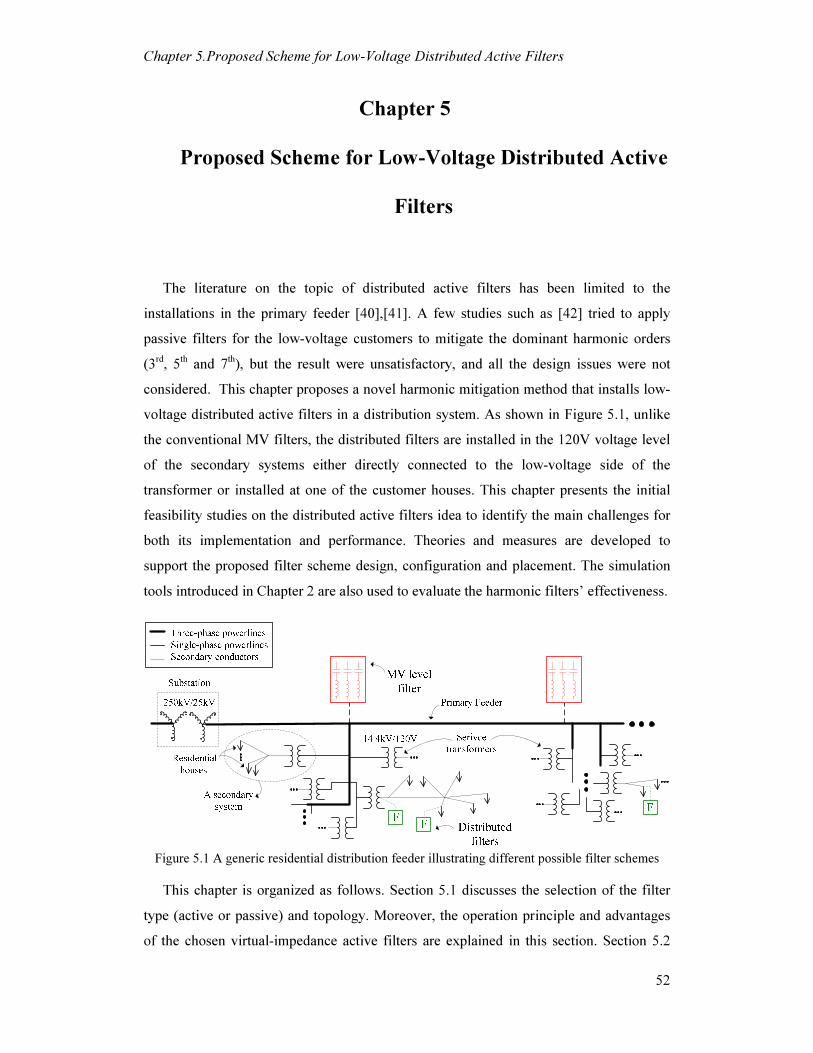
Chapter 5.Proposed Scheme for Low-Voltage Distributed Active Filters
52
Chapter 5
Proposed Scheme for Low-Voltage Distributed Active
Filters
The literature on the topic of distributed active filters has been limited to the
installations in the primary feeder [40], [41]. A few studies such as [42] tried to apply
passive filters for the low-voltage customers to mitigate the dominant harmonic orders
(3rd, 5th and 7th), but the result were unsatisfactory, and all the design issues were not
considered. This chapter proposes a novel harmonic mitigation method that installs low-
voltage distributed active filters in a distribution system. As shown in Figure 5.1, unlike
the conventional MV filters, the distributed filters are installed in the 120V voltage level
of the secondary systems either directly connected to the low-voltage side of the
transformer or installed at one of the customer houses. This chapter presents the initial
feasibility studies on the distributed active filters idea to identify the main challenges for
both its implementation and performance. Theories and measures are developed to
support the proposed filter scheme design, configuration and placement. The simulation
tools introduced in Chapter 2 are also used to evaluate the harmonic filters’ effectiveness.
Figure 5.1 A generic residential distribution feeder illustrating different possible filter schemes
This chapter is organized as follows. Section 5.1 discusses the selection of the filter
type (active or passive) and topology. Moreover, the operation principle and advantages
of the chosen virtual-impedance active filters are explained in this section. Section 5.2

Chapter 5.Proposed Scheme for Low-Voltage Distributed Active Filters
53
investigates the installment issues for a distributed filter scheme. Theoretical analyses are
performed to study the possible filter configurations and placement options. Section 5.3
presents the results of the secondary system simulation studies where different filter
installation options are assessed for a typical North American secondary distribution
system. In addition, the overall harmonic mitigation effectiveness of the proposed
distributed filters scheme is evaluated by using primary system simulations in Section 5.4.
Both of the actual and ideal feeders are studied with some supporting sensitivity analyses
to achieve a better understanding of the overall performance of the filters in suppressing
the distribution system harmonics. Section 5.5 determines the final specification of the
distributed filters schemes for both studied feeders in accordance with the defined
mitigation objectives presented in Chapter 2. Finally, the main findings of this chapter are
summarized in section 5.6.
5.1 Filter Type and Topology Selection
Section 5.1.1 explains why the active filters are preferred to their passive counterparts
for the proposed distributed scheme. In addition, section 5.1.2 also discusses the reason
behind selecting the virtual-impedance active filters instead of the other conventional
types of active filter.
5.1.1 Active versus Passive Filters
When it concerns the distributed filter schemes, the active filters are usually preferred
over the passive ones. In fact, the virtual-impedance type of active filters is selected for
the proposed mitigation method (The reason of choosing this type of active filters will be
discussed in the next section). This type of active filters sinks the harmonic currents by
exhibiting a low resistive impedance at all of the harmonic frequencies while appearing
as an open-circuit for the fundamental frequency component [40]- [41], [43]- [44]. Such
active harmonic filters will at least have the following advantages over the passive
counterparts when applied for the distributed scheme:
• Multiple branches of passive filters are needed to mitigate all harmonic orders
(3rd, 5th, 7th, etc.), while it can be all done by a single active device. Overall, the

Chapter 5.Proposed Scheme for Low-Voltage Distributed Active Filters
54
size of the active filter will be considerably less than its passive counterpart for
this application.
• Since the virtual-impedance active filters appear as resistive impedances to the
system, they will not cause harmonic amplification due to a parallel resonance.
• The typical secondary system impedance values are quite low so that very low
filter impedances are also needed. In contrast to the passive filters, such active
filters establish their equivalent impedance virtually through a power electronics
circuit and its control system. While for the passive counterparts, the required low
filter impedance has to be established physically where it already includes the
series resistance of their capacitor and inductors as well as the residual impedance
due to the components detuning.
In addition, since the filters are supposed for a low voltage application, the price of
active filter power-electronic devices will also become reasonable compared to their
passive counterparts.
5.1.2 Virtual-impedance Active Filter
Shunt active filters can be generally classified into two groups based on their control
principle as below [19],
1. The traditional active filters (with a current-detection based control): It appears as a
controlled current source injecting a compensating harmonic current into the system to
cancel the harmonic currents flowing from the downstream side (Figure 5.2 (a)).
2. The virtual-impedance active filters (with a voltage-detection based control): This
type also behaves as a controlled current source in the circuit but instead of injecting the
compensating current, it sinks a current proportional to the harmonic part of the filter
voltage (vh in Figure 5.2 (b)) so that a virtual resistive impedance is established to absorb
the harmonics from both upstream and downstream sides of the system (Figure 5.2 (b)).
For the fundamental frequency, the filter acts as an open circuit (The equivalent circuit of
such filters is depicted in Figure 5.4(b)) [40]- [41], [43]- [44].

Chapter 5.Proposed Scheme for Low-Voltage Distributed Active Filters
55
if =-kih
k ≈1
Upstream Downstreamih
(a) (b)
Figure 5.2 Simplified schematic of a shunt active filter with (a) current-detection based
control (traditional type) (b) voltage-detection based control (virtual-impedance).
The virtual-impedance active filter (second type) is selected for the proposed
distributed filter scheme because of the following advantages over the traditional type,
• Unlike the current-detection based type, the virtual-impedance filter can be also
installed at one of the houses since of its ability to attract the harmonics from the
other customers’ houses.
• Whether the filter being installed at service transformer or one of the houses,
with the virtual-impedance type, a portion of the harmonics from the other parts
of system (associated with other service transformers) will be also mitigated. This
fact will be verified by the simulation results that will be later presented in section
5.4.1.
• As shown in Figure 5.2 (a), the traditional active filters require measuring of the
downstream power-line current. The virtual-impedance filter does not require
such current sensors.
The only remaining issue with the virtual-impedance active filters is the fact that they
have to establish a lower impedance than the system’s one to achieve an effective
harmonic suppression. Figure 5.3 shows an impedance frequency scan of a typical
secondary system measured at a house (This frequency scan is obtained by both
simulation and analytical analysis. For more details of the system refer to Figure 5.11).

Chapter 5.Proposed Scheme for Low-Voltage Distributed Active Filters
56
1st 3rd 5th 7th 9th 11th 13th 15th0
0.1
0.2
0.3
0.4
Harmonic order
Syst
em
Im
ped
ance(
Ω)
Simulation
Analytical
Figure 5.3 Frequency scan at a house of a typical secondary feeder (House #3 in Figure 5.11)
Figure 5.3 shows that the system impedance is quite low. Therefore, the ability of
establishing low virtual impedance values must be considered in the design of such active
filters (In the consequent sections of this chapter, the impedance values required for an
effective mitigation will be studied). Traditionally, it has not been a concern for the
design of the virtual-impedance active filters, since all the previous studies have
considered them only for the primary-level systems (MV) where the system impedance is
not too low. Moreover, too low filter impedances have been always deliberately avoided
to prevent filter overheating [40], [41].
Figure 5.4(a) shows a very simplified schematic of the circuit and control diagram of a
single-phase virtual-impedance active filter [43]. In the steady-state condition, the filter
current (if in Figure 5.4(a)) will approximately equals the reference current (if,ref in Figure
5.4 (a)). So that,
V h= = K v ⇒f f,ref fi i i
( 5.1 )
where KV is the control loop gain factor as shown in Figure 5.4(a). From ( 5.1 ), the
equivalent harmonic impedance of the filter can be calculated (Figure 5.4(b)):
f f VZ ( ) = Z ( ) = 1/K / ⇒h fh v i h ( 5.2 )
As a result, the gain factor in the control loop (KV) determines the obtained virtual
impedance (Zf). The higher this gain factor, the lower filter impedance is achieved (For
example to obtain Zf=0.02Ω, KV must be at least 50). However, too high values of KV
may cause some stability, etc. issues for the filter converter control mechanisms. The
possible issues and their solutions are supposed to be studied in the next level of this
research project devoted to the design and implementation of the proposed virtual-
impedance active filters.

Chapter 5.Proposed Scheme for Low-Voltage Distributed Active Filters
57
(a)
(b)
Figure 5.4 The single-phase virtual-impedance active filter (a) Circuit schematic and control
diagram (b) Equivalent system
5.2 Filter Installment Issues
This section investigates the available options and essential consideration of installing the
distributed filters in a North American distribution system. Section 5.2.1 studies the
option of installing the filters directly between the two phases to save in number of filters.
Different available locations to place the filter within the system are also discussed in
Section 5.2.2.
5.2.1 Double- phase Connection
The North American secondary distribution systems have a double-phase circuit structure.
Each appliance in a house is either connected to one of the phases and neutral (120V) or
directly between the two phases (240V) [45]. With such double-phase configuration, two
options will be possible for equipping the secondary system with these filters. The first
option is to connect two separated filters each of them between one phase and neutral
(Figure 5.5(b)). The other option is to connect a single filter directly between phases A
and B (Figure 5.5(c)). Intuitively, the first choice is certainly effective; however,
evaluating the performance of the second option needs a deeper analysis.

Chapter 5.Proposed Scheme for Low-Voltage Distributed Active Filters
58
,h aI
,h pI
,h bI
: :1 α α
(a)
',h aI
',h pI
',h bI
: :1 α α
(b)
",h aI
",h pI
",h bI
: :1 α α
(c)
Figure 5.5 Different possible filter installment options: (b) Two single-phase connected filters
(c) One double-phase connected filter.
Figure 5.6 shows the equivalent circuits used to analytically evaluate and compare the
effectiveness of the aforementioned options. In the figure, Zs and Zp are the secondary-
and primary-winding impedances respectively (All the impedance values are transferred
to the secondary side). The secondary to primary voltage ratio of the service transformer
is shown by α. Zf, Zl and Zeq,pr are the filter, secondary power-line and primary system
equivalent impedance values, respectively. The current sources of Ih,A and Ih,B are
representing the harmonic currents generated by the nonlinear loads in phases A and B.
The harmonic currents penetrating into the primary system respectively for the two cases
are respectively labeled as I’h,p and I”h,p.
,f aI
,f bI
',h aI
',h pI
',h bI
: :1 α α
(a)
fI
fI
'',h aI
",h pI
",h bI
: :1 α α
(b)
Figure 5.6 Equivalent circuit of system with (a) two single-phase filter (b) one double-phase filter.
When there is no filter in the system, the harmonic current penetrating into the
primary system (Ih,p in Figure 5.5(a)) is,
, , , , ,( ) ( )h p h a h b h A h BI I I I Iα α= + = + ( 5.3)
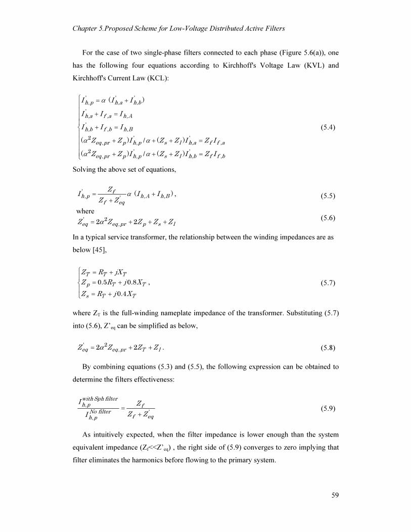
Chapter 5.Proposed Scheme for Low-Voltage Distributed Active Filters
59
For the case of two single-phase filters connected to each phase (Figure 5.6(a)), one
has the following four equations according to Kirchhoff's Voltage Law (KVL) and
Kirchhoff's Current Law (KCL):
' ' ', , ,
', , ,
', , ,
2 ' ', , , ,
2 ' ', , , ,
( )
( ) / ( )
( ) / ( )
h p h a h b
h a f a h A
h b f b h B
eq pr p h p s l h a f f a
eq pr p h p s l h b f f b
I I I
I I I
I I I
Z Z I Z Z I Z I
Z Z I Z Z I Z I
α
α α
α α
= + + =
+ =
+ + + = + + + =
( 5.4)
Solving the above set of equations,
', , ,'
( )fh p h A h B
f eq
ZI I I
Z Z
α= +
+
, ( 5.5)
where ' 2
,2 2eq eq pr p s lZ Z Z Z Zα= + + + ( 5.6)
In a typical service transformer, the relationship between the winding impedances are as
below [45],
0.5 0.8
0.4
T T T
p T T
s T T
Z R jX
Z R j X
Z R j X
= +
= +
= +
, ( 5.7)
where ZT is the full-winding nameplate impedance of the transformer. Substituting ( 5.7)
into ( 5.6), Z’eq can be simplified as below,
' 2,2 2eq eq pr T lZ Z Z Zα= + + . ( 5.8)
By combining equations ( 5.3) and ( 5.5), the following expression can be obtained to
determine the filters effectiveness:
,
'
,
with Sph filterh p f
No filterf eqh p
I Z
Z ZI
=
+
( 5.9)
As intuitively expected, when the filter impedance is lower enough than the system
equivalent impedance (Zf<<Z’eq) , the right side of ( 5.9) converges to zero implying that
filter eliminates the harmonics before flowing to the primary system.

Chapter 5.Proposed Scheme for Low-Voltage Distributed Active Filters
60
For a double-phase connected filter directly between phase A and B, KVL and KCL
principles apply the following set of equations:
" " ", , ,
", ,
", ,
2 " " ", , , ,
( )
2( ) / ( )( )
h p h a h b
h a f h A
h b f h B
eq pr p h p s l h a h b f f
I I I
I I I
I I I
Z Z I Z Z I I Z I
α
α α
= + + =
+ =
+ + + + =
( 5.10)
Solving the above set of equations leads to
", , ,"
( )fh p h A h B
f eq
ZI I I
Z Z
α= +
+
, ( 5.11)
where (7)
" 2 2, ,4 4 2 2 4 4 2eq eq pr p s l eq pr T lZ Z Z Z Z Z Z Zα α= + + + == + + .
( 5.12)
Furthermore, by dividing ( 5.11) over ( 5.5), the final equation for evaluating the
performance of a double-phase connected filter can be further simplified as below,
,
,
with Dph filterh p f
No filter Dphf eqh p
I Z
Z ZI
=
+
, ( 5.13)
where 2,4 4 2
Dpheq eq pr T lZ Z Z Zα= + + . ( 5.14)
The equation ( 5.13) demonstrates that the double-phase connected filter is also able to
eliminate the harmonic penetration into the primary system with a similar theoretical
principle to the single-phase connected filters. Comparing ( 5.8) and ( 5.14) also reveals
that the equivalent system impedance for the double-phase connection is even higher than
the single-phase connected ones; therefore, even a more effective harmonic mitigation
can be achieved with the same filter impedance value!
Due to the obvious advantage of saving in number of filter devices, the double-phase
connection is chosen for the distributed filtering scheme and will be used in all of this
thesis studies. Simulation studies will be also provided in section 5.3.1 to verify the
effectiveness of the double-phase configuration compared to the single-phase ones.

Chapter 5.Proposed Scheme for Low-Voltage Distributed Active Filters
61
5.2.2 Filter Location Options
As depicted in Figure 5.7, each filter can be either installed at the supplying service
transformer or at one of the customer houses. In the previous section, ( 5.11) and ( 5.12)
were derived for assessing the double-phase connected filter performance. When the filter
is attached to the service transformer, there will be no line impedance (Zl) in ( 5.12) and
the equivalent system impedance will be as below,
2,4 4sys eq pr TZ Z Zα= + ( 5.15)
(a) (b) Figure 5.7 The two options for filter location: (a) at service transformer (b) at one of the houses.
The simplified circuit shown in Figure 5.8 is used for analyzing the case when the
filter is installed in a house. I’h,A and I’h,B are the current sources representing the
harmonic currents generated by the house which filter is installed at. The harmonic
currents injected by the other houses are modeled as Ih,A and Ih,B. ZLs and ZLb are the
impedances of secondary and the service conductor of the house with the filter,
respectively. In this simplified circuit, the impedances of other service conductors and
linear home appliances are ignored since of their negligible effect on the harmonic flow.
",h pI : :1 α α
,h AI
,h BI ',h BI
',h AI
Figure 5.8 The equivalent circuit of system when installing filter at one of the houses.
By ignoring the harmonic currents produced by the house with filter (I`h,A and I`h,B),
the equivalent circuit can be even more simplified as shown in Figure 5.9. As depicted in

Chapter 5.Proposed Scheme for Low-Voltage Distributed Active Filters
62
the figure, the equivalent filter branch impedance includes the service conductor
impedance as well as the filter impedance.
",h pI : :1 α α
,h AI
,h BI
Figure 5.9 The equivalent filter branch when installing filter at one of the houses, simplified with
ignoring the harmonic currents generated inside that house.
Based on this simplified equivalent circuit (Figure 5.9), one can use a similar equation
to ( 5.11) to assess the filter effectiveness as below,
, ,
,
,
Filteredh p eq F
No filtereq F sysh p
I Z
Z ZI
=
+
, ( 5.16)
where the equivalent system impedance is
2,4 4 2sys eq pr T LsZ Z Z Zα= + + , ( 5.17)
And the equivalent filtering impedance (The impedance of equivalent filter branch
shown in Figure 5.9) is,
,
2eq F F LbZ Z Z= + ( 5.18)
In conclusion, although placing the filter in a house leads to a higher equivalent
filtering impedance compared to service transformer placement; however, the system
equivalent impedance will be also higher. Anyways, the closest house to the service
transformer must be equipped with the filter to achieve the most effective harmonic
suppression (the closest house will bring the lowest service conductor impedance (ZL2)
leading to lowest filtering impedance (Zf,eq)).
The above analyses also reveal that with any of the location options, just one filter is
enough for each secondary system to achieve an effective harmonic mitigation.
Simulation results will be also provided in section 5.3.2 to evaluate and compare different
filter location options. Table 5.1 compares the two location options in summary.

Chapter 5.Proposed Scheme for Low-Voltage Distributed Active Filters
63
Table 5.1 Comparison of the two filter location options
Filter location
At the service transformer At the closest
house
Effective harmonic mitigation
Providing higher equivalent system impedance
Providing lower equivalent filtering impedance
5.3 Simulation Studies on Secondary System
This section conducts the simulation studies on the secondary level of distribution
systems in support of the theoretical discussions presented in this chapter so far. The
studies are mainly aimed to answer the following questions regarding a distributed active
filter scheme for a North American distribution system:
1. How is the filters effectiveness when they are directly connected between the two
phases?
2. Is a single filter really enough for each secondary system? If so, what are the
optimum locations for installing the filters?
3. What is the impact of the secondary system configuration?
4. How much the filter impedance value affects the harmonics elimination?
As depicted in Figure 5.10, three types of configurations can be found for a secondary
distribution system in North America: cascade, parallel or a combination of parallel and
cascade. The last two configurations are more common compared to the first one.
(a) (b) (c) Figure 5.10 Different configurations of a secondary distribution system (a) cascade (b) parallel (c) combination of parallel and cascade.
In order to avoid too much complexity in the simulations, the parallel configuration is
chosen for most of the simulations as the typical system. Consisting of a service
transformer supplying five residential houses as shown in Figure 5.11, the typical system
is sufficient for most of the studies such as comparing different filter configurations, filter

Chapter 5.Proposed Scheme for Low-Voltage Distributed Active Filters
64
installation at the transformer, required filter impedance, etc. Additionally, section 5.3.2.1
will also study the systems with a more generalized configuration to verify the
conclusions obtained via the typical system regarding the optimum house for filter
placement.
Figure 5.11 The typical secondary system chosen for simulation studies.
Table 5.2 gives the parameters of the typical system used in the simulations. Figure
5.12 and Figure 5.13 show the circuits for performing the load flow and harmonic load
flow simulations of the system by employing an in-house HLF program [29]. At
harmonic frequencies, linear loads in a house are represented as impedances (Zha , Zhb and
Zhab in Figure 5.12) ,while, nonlinear loads are modeled as harmonic current sources(Iha
and Ihb in Figure 5.13). The modeling method to obtain the equivalent harmonic current
sources and impedances of each house is based on the similar bottom-up approach as
described in Chapter 2. Since the models are time-varying, the results are obtained for
different hours during a day.
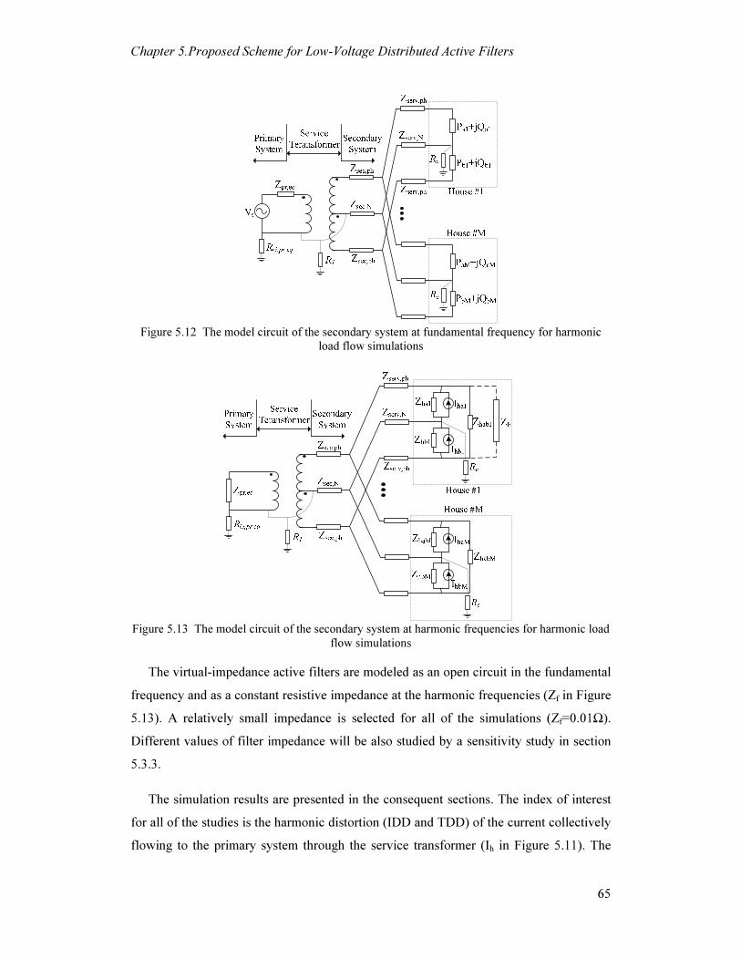
Chapter 5.Proposed Scheme for Low-Voltage Distributed Active Filters
65
Figure 5.12 The model circuit of the secondary system at fundamental frequency for harmonic
load flow simulations
Figure 5.13 The model circuit of the secondary system at harmonic frequencies for harmonic load
flow simulations
The virtual-impedance active filters are modeled as an open circuit in the fundamental
frequency and as a constant resistive impedance at the harmonic frequencies (Zf in Figure
5.13). A relatively small impedance is selected for all of the simulations (Zf=0.01Ω).
Different values of filter impedance will be also studied by a sensitivity study in section
5.3.3.
The simulation results are presented in the consequent sections. The index of interest
for all of the studies is the harmonic distortion (IDD and TDD) of the current collectively
flowing to the primary system through the service transformer (Ih in Figure 5.11). The

Chapter 5.Proposed Scheme for Low-Voltage Distributed Active Filters
66
reduction of such index can exhibit the effectiveness of different filtering scenarios.
Section 5.3.1 presents the results for verifying performance of the double-phase
connected filter. Some case study results are shown in section 5.3.2 to evaluate different
filter placement options. Finally, a sensitivity study is conducted in section 5.3.3 to
investigate the impact of different filter impedance values.
Table 5.2 Simulation system parameters
System parameter Value
Grounding resistance (RG,pr,eq) a 0.4560+0.2963j Ω
Primary equivalent impedance (Zpr,eq) b 0.4806+2.5833j Ω Primary system
Primary voltage source (Vs) 14.4kV
Voltage ratio 14.4kV/120V/120V
kVA rating 37.5 kVA
Impedance 2% pu
Resistance 1.293% pu
Service transformer
Grounding resistance (RT) 12 Ω
Secondary conductor phase Impedance (Zsec,ph) 0.21+0.094j Ω/km
Secondary conductor neutral Impedance (Zsec,N) 0.55+0.365j Ω/km
Service conductor phase Impedance (Zserv,ph) 0.34+0.137j Ω/km
Service conductor neutral Impedance (Zserv,N) 0.55+0.365j Ω/km
House grounding resistance(RC) 1 Ω
Secondary system
Each house daily average power 1kW
at fundamental frequency ∞ Filter virtual impedance at harmonics
0.01 Ω
a This impedance is obtained as the equivalent of an MGN distribution system grounding resistance value. For more details, refer to [7]. b This value is in fact varied depending where the service transformer is connected to the feeder. To avoid complexity, a typical value of substation impedance is used here [28] (Please note that this impedance have a very negligible effect on the studies , since when transferred to secondary side of the transformer, it will be so much smaller than other secondary system components impedance).
5.3.1 Double-phase versus Single-phase Connection
The two different options for installing the filter in a secondary system with the double-
phase scheme (as discussed in section 5.2.1) are investigated by selecting the following
case studies.
1. The typical secondary system (Figure 5.11) normal operation without any filter.
2. Two single filters are installed separately one to phase A and the other to phase B at
house #3 of the system (Figure 5.11).
3. One double-phase filter connected directly between phase A and B of the same house.

Chapter 5.Proposed Scheme for Low-Voltage Distributed Active Filters
67
The daily profile of current TDD and average value of IDD associated with the
harmonic current penetrating to primary system for all the cases are shown in Figure 5.14.
The results once again confirm the effectiveness of double-phase connection as
anticipated by the theoretical discussions in section 5.2.1.
1 5 9 13 17 210
1
2
3
4
5
Time(hour)
Curr
ent
TD
D(%
)No filter
with two Single-phase filters
with one Double-phase filter
(a)
3rd 5th 7th 9th 11th 13th 15th TDD0
0.5
1
1.5
2
Dai
ly A
vera
ge C
urr
en
t ID
D(%
)
Harmonic order
No filter
with two Single-phase filters
with one Double-phase filter
(b)
Figure 5.14 Comparison of single-phase and double-phase filter configurations in mitigation of harmonic currents penetrating the primary system (a) Daily profile of Current TDD (b) Daily
average value IDD.
5.3.2 Filter Placement in the Secondary System
This section studies different filter placement options in a secondary system. The first
step is to compare filter installation at the service transformer and the houses in the
typical system (with the parallel configuration as in Figure 5.11). Then, additional
analytical and simulation results are provided in 5.3.2.2 by considering a more
generalized system configuration.
5.3.2.1. In the Typical System
The following cases are studied,
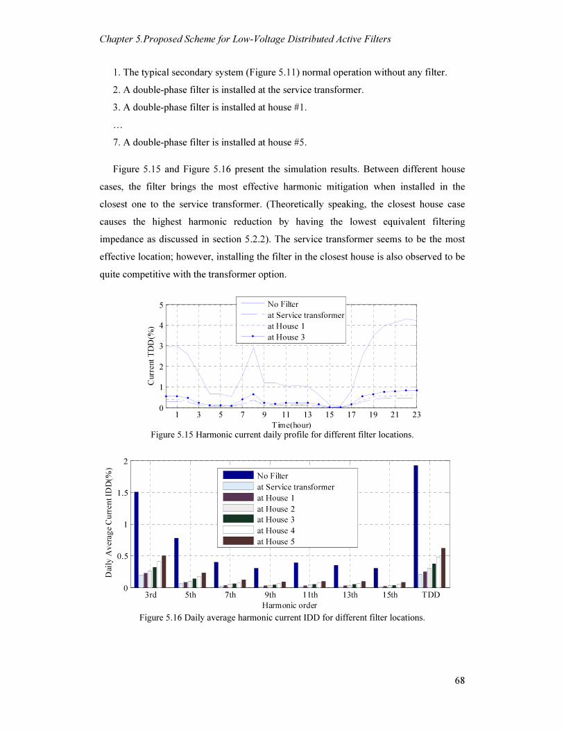
Chapter 5.Proposed Scheme for Low-Voltage Distributed Active Filters
68
1. The typical secondary system (Figure 5.11) normal operation without any filter.
2. A double-phase filter is installed at the service transformer.
3. A double-phase filter is installed at house #1.
…
7. A double-phase filter is installed at house #5.
Figure 5.15 and Figure 5.16 present the simulation results. Between different house
cases, the filter brings the most effective harmonic mitigation when installed in the
closest one to the service transformer. (Theoretically speaking, the closest house case
causes the highest harmonic reduction by having the lowest equivalent filtering
impedance as discussed in section 5.2.2). The service transformer seems to be the most
effective location; however, installing the filter in the closest house is also observed to be
quite competitive with the transformer option.
1 3 5 7 9 11 13 15 17 19 21 230
1
2
3
4
5
Time(hour)
Curr
ent
TD
D(%
)
No Filter
at Service transformer
at House 1
at House 3
Figure 5.15 Harmonic current daily profile for different filter locations.
3rd 5th 7th 9th 11th 13th 15th TDD0
0.5
1
1.5
2
Dai
ly A
vera
ge C
urr
en
t ID
D(%
)
Harmonic order
No Filter
at Service transformer
at House 1
at House 2
at House 3
at House 4
at House 5
Figure 5.16 Daily average harmonic current IDD for different filter locations.

Chapter 5.Proposed Scheme for Low-Voltage Distributed Active Filters
69
5.3.2.2 In a Generalized Configuration
Studies in the previous section revealed that the closest house to the service transformer
is the most effective one among the other houses to locate the filter in a parallel
configured secondary system. This section considers a more generalized system as
depicted in Figure 5.17. There are two groups of houses supplied by the transformer.
Apparently, the house with the shortest service conductor is the best option inside each
group (Location A in the first group and location B in the second one). In this section,
analytical estimations and simulation studies are performed to identify which of these two
options (Locations A and B) is the most effective filter location.
Figure 5.17 A generalized secondary distribution system with a combined parallel-cascade configuration.
In order to cover most of the common North American secondary systems, several
cases including different combinations of house numbers in each group and typical
minimum and maximum of secondary conductor lengths are considered as follows.
1. Distribution of house numbers in each group: N1=7 & N2=3, N1=5 & N2=5, N1=3
& N2=7,
2. First secondary conductor length: L1= 10m, 30m,
3. Second secondary conductor length: L2= 20m, 60m.
The service conductor length of the houses with filter (which are the ones with
shortest service conductors) is considered 10m for all the cases. Lengths of the service
conductors of other houses will have negligible effect on harmonic flow results so that
are just randomly selected for each case. The filter effectiveness at both locations A and
B is assessed by measuring the harmonic reduction percentage. Table 5.3 shows the
results. Analytical studies are only presented for the 3rd harmonic, where associated

Chapter 5.Proposed Scheme for Low-Voltage Distributed Active Filters
70
simulation results are also presented both for 3rd harmonic and all the harmonics (TDD).
Appendix D.1 describes the details of the analytical estimation procedure.
Table 5.3 The harmonic reduction percentage for comparing filter locations A and B including several cases with different length of lines and number of houses.
3
3
(%)Filteredrd
NoFilterrd
IDD
IDD
(%)FilteredI
NoFilterI
TDD
TDD
Secondary system
configuration parameters Analytical Estimation
Simulation Result
Simulation Result
Filter Location Filter Location Filter Location Case No.
N1 N2 L1
(m) L2
(m) A B A B A B
1 7 3 10 20 20.0 26.0 18.5 20.5 16.2 18.4
2 7 3 10 60 20.0 34.8 18.5 23.2 16.2 21.2
3 7 3 30 20 17.5 23.0 16.2 18.2 14.2 16.3
4 7 3 30 60 17.5 31.5 16.2 21.0 14.2 19.3
5 5 5 10 20 20.0 23.5 18.5 21.9 16.2 19.9
6 5 5 10 60 20.0 28.7 18.5 28.0 16.2 26.1
7 5 5 30 20 17.5 20.8 16.2 19.5 14.3 17.8
8 5 5 30 60 17.5 26.0 16.2 25.4 14.3 23.8
9 3 7 10 20 20.0 21.0 18.5 25.0 16.3 22.8
10 3 7 10 60 20.0 22.6 18.5 35.6 16.3 33.2
11 3 7 30 20 17.5 18.6 16.2 22.2 14.3 20.3
12 3 7 30 60 17.5 20.5 16.2 32.3 14.3 30.2
The results of all the cases show that the filter is always more effective at location A
compared to location B. In conclusion, when installing the filter at one of the houses of a
secondary distribution system, the most effective mitigation is achieved by placing the
filter in the closest house to the service transformer disregard of the system configuration.
Interestingly, the results also verify the fact that most of the system configuration
parameters such as number of houses and all the conductor lengths (except of the first
secondary conductor and the service conductor of the house with filter) do not affect the
filtering performance considerably, when the filter is located in the closest house to
service transformer (location A). For example, the simulation results of cases 3, 4, 7, 8,
11 and 12 with the similar secondary lengths (L1) of 30m and service conductor lengths
of 10m are quite similar.
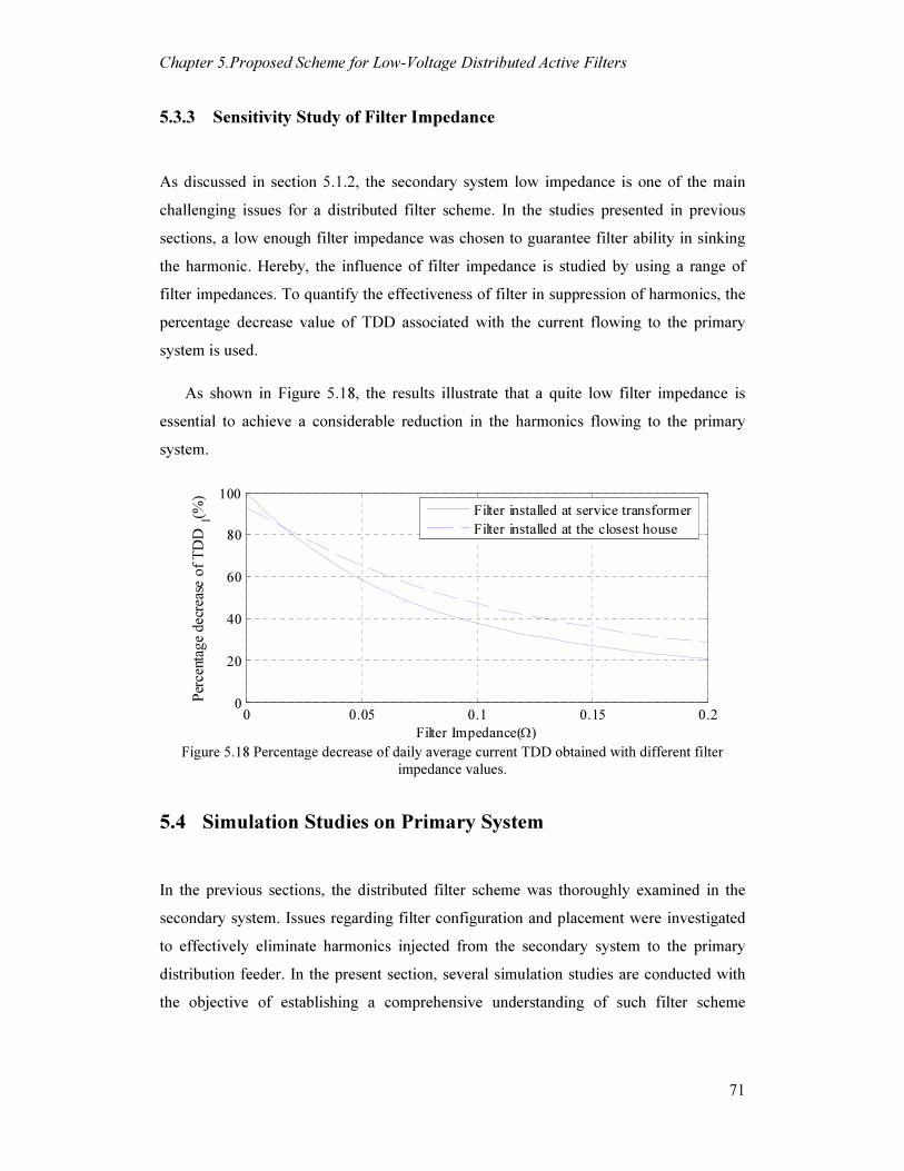
Chapter 5.Proposed Scheme for Low-Voltage Distributed Active Filters
71
5.3.3 Sensitivity Study of Filter Impedance
As discussed in section 5.1.2, the secondary system low impedance is one of the main
challenging issues for a distributed filter scheme. In the studies presented in previous
sections, a low enough filter impedance was chosen to guarantee filter ability in sinking
the harmonic. Hereby, the influence of filter impedance is studied by using a range of
filter impedances. To quantify the effectiveness of filter in suppression of harmonics, the
percentage decrease value of TDD associated with the current flowing to the primary
system is used.
As shown in Figure 5.18, the results illustrate that a quite low filter impedance is
essential to achieve a considerable reduction in the harmonics flowing to the primary
system.
0 0.05 0.1 0.15 0.20
20
40
60
80
100
Filter Impedance(Ω)
Per
cent
age
dec
reas
e o
f T
DD
I(%)
Filter installed at service transformer
Filter installed at the closest house
Figure 5.18 Percentage decrease of daily average current TDD obtained with different filter
impedance values.
5.4 Simulation Studies on Primary System
In the previous sections, the distributed filter scheme was thoroughly examined in the
secondary system. Issues regarding filter configuration and placement were investigated
to effectively eliminate harmonics injected from the secondary system to the primary
distribution feeder. In the present section, several simulation studies are conducted with
the objective of establishing a comprehensive understanding of such filter scheme

Chapter 5.Proposed Scheme for Low-Voltage Distributed Active Filters
72
effectiveness in mitigation of the whole system harmonics. Different feeder types and
conditions are included in the studies to answer the following important questions:
1. Is it essential to equip all of the service transformers in a feeder with the distributed
filters to achieve an effective harmonic suppression? If not, how does this mitigation
scheme improve with increasing the number of installed filters?
2. How the feeder configuration and the distribution of loads affect the distributed
filters performance?
3. What is the required filters impedance range to reach a reasonable system-wide
harmonic mitigation?
The studies are conducted on both the real and ideal feeders introduced in Chapter 2.
Each of the secondary systems supplied by the feeder is modeled when equipped with the
distributed filters. System modeling and simulation techniques are explained in details in
in Chapter 2 and Appendix A. Indices of interest are also adopted according to Chapter 2.
The simulation results accompanied with the related discussions are presented in sections
5.4.1 through 5.4.3.
5.4.1 Base Results
This section presents the initial results of equipping the real and ideal feeders with the
distributed filters. The simulations are performed for different percentages of secondary
systems equipped with such filters. The both filter location options are included for each
feeder study: in one case, the filters are directly attached to the service transformers,
while the nearest houses to the service transformers are chosen as the filters locations for
the other case (For more details regarding filter placement options refer to sections 5.2.2
and 5.3.2). The filter impedance value of Zf=.01Ω is chosen for these basic studies. The
other impedance values will be examined by the sensitivity study performed in section
5.4.3.
As shown through Figure 5.19 and Figure 5.20, the base results confirm that for both
filter locations and for both feeders the distributed filters can be significantly effective in
suppression of feeder harmonics. Even with only 30% of the system equipped with the
filters, a noticeable reduction of the harmonic indices is observed.

Chapter 5.Proposed Scheme for Low-Voltage Distributed Active Filters
73
0 10 20 30 40 50 60 70 80 90 1000
2
4
6
8
10
Percentage of service transformers equipped with distributed filters (%)
TD
DI i
n S
ub
stati
on
(%)
Actual feeder - Filters installed at service transformer
Actual feeder - Filters installed at the closest house
Ideal feeder - Filters installed at service transformer
Ideal feeder - Filters installed at the closest house
Figure 5.19 Current TDD in substation (daily 95% percentile value) versus percentage of service
transformers equipped with distributed filters.
At low percentages of filters installation, the actual feeder exhibits a different
behavior from the ideal feeder. Especially for voltage THD as shown in Figure 5.20, that
with lower percentages than 10%, THD is even somehow increased inside the actual
feeder. As introduced in Chapter 2, the actual feeder (differently from the ideal one)
have several sections of underground cable with significant shunt capacitive admittance
values and this phenomenon is due to the existence of these shunt capacitances in the
system (For more explanations refer to Appendix D.2). To verify this scenario, an
additional simulation case is also conducted by removing the shunt capacitance of
underground cables inside the actual feeder. This extra case is added to Figure 5.21 and
Figure 5.22, where the percentage decrease of TDDI and THDV are plotted. The results
also demonstrate that the major cause of the difference between the real and ideal feeders
at low filtering percentages is the shunt capacitance of underground cables.
0 10 20 30 40 50 60 70 80 90 1000
5
10
15
20
Percentage of service transformers equipped with distributed filters (%)
TH
DV a
vera
ge o
ver
th
e fe
eder(
%)
Actual feeder - Filters installed at service transformer
Actual feeder - Filters installed at the closest house
Ideal feeder - Filters installed at service transformer
Ideal feeder - Filters installed at the closest house
Figure 5.20 Voltage THD (daily 95% percentile value) average along feeder versus percentage of
service transformers equipped with distributed filters.

Chapter 5.Proposed Scheme for Low-Voltage Distributed Active Filters
74
In addition, a very attractive illustration of the Figure 5.21 and Figure 5.22 is
highlighted by the dashed red lines added to the plots. For those linear dashed lines, the
percentage decrease of TDDI (or THDV) is exactly equal to the filtering percentage.
Comparing the obtained results with such dashed lines indicates that the percentage
harmonic decrease achieved by the distributed filters in the both feeders can be much
higher than the filtering percentage. It is due to the fact that each filter not only eliminates
the harmonics generated inside its own secondary system, but also contributes to the
system-wide harmonic mitigation by attracting the harmonics flowing from the other
service transformers of the feeder. Such ability of sinking harmonics from both
downstream and upstream sides of the system is one of most important merits of the
chosen virtual-impedance active filters compared to their traditional counterparts with the
current-detection based control as discussed in section 5.1.2. If the traditional active
filters were chosen for the distributed filter scheme, then the harmonic reduction
percentage could have only been reaching as high as the red dashed lines in the figures.
0 10 20 30 40 50 60 70 80 90 1000
20
40
60
80
100
Percentage of service transformers equipped with distributed filters (%)
Per
cen
tag
e d
ecre
ase
of
TD
DI(%
)
Actual feeder
Actual feeder- powerlines shunt capacitance removed
Ideal feeder
Figure 5.21 Percentage decrease of substation current TDD versus percentage of secondary
systems equipped with the distributed filters installed in service transformer.

Chapter 5.Proposed Scheme for Low-Voltage Distributed Active Filters
75
0 10 20 30 40 50 60 70 80 90 1000
20
40
60
80
100
Percentage of service transformers equipped with distributed filters (%)
Per
cen
tag
e d
ecre
ase
of
TH
DV(%
)
Actual feeder
Actual feeder- powerlines shunt capacitance removed
Ideal feeder
Figure 5.22 Percentage decrease of feeder average voltage THD versus percentage of secondary
systems equipped with the distributed filters installed in service transformer.
5.4.2 Sensitivity Study of Feeder Parameters
This section presents the sensitivity study to assess the influence of the feeder
characteristics and loads distribution on the distributed filters performance. Simulation
results for the following cases are compared in Figure 5.23.
I. The ideal feeder normal condition without any changes.
II. The ideal feeder with the power-line sections length decreased from 1000m to
500m.
III. The ideal feeder with the power-line sections length increased from 1000m to
2000m.
IV. The ideal feeder with reducing the number of supplied service transformers from
450 to 225.
V. The ideal feeder when all the feeder conductors are converted from overhead lines
to underground cables.
VI. The ideal feeder where all of the service transformers are moved to end of the
feeder.
VII. The ideal feeder where all of the service transformers are moved to the middle of
the feeder.

Chapter 5.Proposed Scheme for Low-Voltage Distributed Active Filters
76
25% 50% 75% 100%0
20
40
60
80
100
Percentage of service transformers Equipped with Distributed Filters
Per
cen
tag
e d
ecre
ase
of
TD
DI(%
)
25% 50% 75% 100%0
20
40
60
80
100
Per
cen
tag
e d
ecre
ase
of
TH
DV(%
)
I-Ideal feeder
II-Ideal feeder with shorter lines
III-Ideal feeder with longer lines
IV-Ideal feeder with half number of service transformers
V-Ideal feeder with underground cables
VI-Ideal feeder with all loads at the end
VII-Ideal feeder with all loads in the middle
VIII-Actual Feeder
Figure 5.23 Percentage decrease values of current TDD and voltage THD versus percentage of
service transformers equipped with distributed filters for different feeder characteristics.
No significant difference among the different cases is observed especially as the
percentage of filtered secondary systems increases. Promisingly, the results illustrate that
for any feeder with only equipping 25% of service transformers with the distributed
filters, at least 50% of harmonics pollution can be mitigated.
5.4.3 Sensitivity Study of Filter Impedance
In all of the results shown in the previous sections, the filters impedances were chosen to
be Zf=0.01Ω. This section presents the results to study the sensitivity of distributed
filters effectiveness to their impedance value. Simulations are including a range of filter
impedances from 0.001 to 2Ω installed on both of the real and ideal feeder. The results
are all shown in Figure 5.24 where the filters are connected directly to service
transformers. The results of the other case associated with installation of filters at the
closest house are similar and can be found in Appendix D.3.

Chapter 5.Proposed Scheme for Low-Voltage Distributed Active Filters
77
0 0.5 1 1.5 20
20
40
60
80
100
Filter Impedance (Ω)
Per
centa
ge
decr
ease
of
TD
DI(%
)
75%
50%
25%
100%
0 0.5 1 1.5 2
0
20
40
60
80
100
Filter Impedance (Ω)
Per
centa
ge
decr
ease
of
TH
DV(%
)
75%
50%
25%
100%
(a) (b)
0 0.5 1 1.5 20
20
40
60
80
100
Filter Impedance (Ω)
Per
centa
ge
decr
ease
of
TD
DI(%
)
75%
50%
25%
100%
0 0.5 1 1.5 2
0
20
40
60
80
100
Filter Impedance (Ω)
Per
centa
ge
decr
ease
of
TH
DV(%
)
75%
50%
25%
100%
(c) (d)
Figure 5.24 Percentage decrease of current TDD and voltage THD versus filter impedance including four different percentages of service transformers equipped with virtual-impedance distributed filters (a) (b) Ideal feeder (c)(d) Actual feeder (The filters are installed directly at service transformers for all the cases).
Comparing the above results with the ones presented in section 5.3.3, the distributed
filters performance in mitigating the harmonics in the primary system is found to be less
sensitive to filter impedance compared to the secondary system study (see Figure 5.18).
Indeed, a wider range of impedances can bring an effective harmonic mitigation. For
example, according to Figure 5.18 at least an impedance value of 0.1Ω is required for the
filter to eliminate 40% of harmonics generated in its own secondary system; however, the
results presented here, reveal that equipping 50% of service transformers by filters of
around 0.5 Ω impedances can mitigate at least 40% of the feeder harmonic indices.
This significant difference between the primary and secondary system studies is once
again demonstrating the effectiveness of virtual-impedance distributed active filters
reflected in the primary system of distribution system. As mentioned in the previous
sections, such filters not only suppress harmonic currents generated by their own

Chapter 5.Proposed Scheme for Low-Voltage Distributed Active Filters
78
secondary system, but also sink the harmonics flowing from other service transformers in
the system.
5.5 Final Design Specifications
According to the conducted studies presented in this chapter, the final design
specifications of distributed active filters for both of the real and ideal feeders are derived.
The system-wide harmonic mitigation objective defined in Chapter 2 is adopted as the
design criteria.
Two key variables must be determined to finalize the design of distributed active
filters. The first is the number of the required filters and the second is the maximum
permissible equivalent impedance for each device. In order to specify these two variables,
the results of the previous section studies which presented the mitigation performance
obtained by different number of filters and impedance values can be interpolated. Shown
in Table 5.4 are the maximum allowable impedance values necessary to achieve the
mitigation objective for the different cases. As the results show, the more number of
installed filters, the higher value the filters impedances are permitted to be. For most of
the cases, at least 35% of secondary systems must be equipped with the filters; otherwise,
the defined mitigation goal is not achieved.
Table 5.4 The maximum allowable filter impedance values for different percentage of secondary systems equipped with filters to accomplish the system-wide harmonic mitigation objective in
both of the real and ideal feeders.
Maximum allowable filter impedance (Ω)
Percentage of secondary systems
equipped with filters 10% 20% 25% 30% 35% 40% 50% 70% 90% 100%
At service transformer
- - 0.02 0.055 0.08 0.1 0.135 0.205 0.265 0.295 Ideal
Feeder At the closest house
- - - - 0.045 0.07 0.115 0.195 0.265 0.295
At service transformer
- - - - 0.06 0.08 0.11 0.17 0.225 0.25 Actual feeder At the
closest house
- - - - - 0.025 0.09 0.165 0.23 0.26
In order to save in the number of filters, installation percentages of less than 40% are
selected for the final design specifications. The final design characteristics for the two

Chapter 5.Proposed Scheme for Low-Voltage Distributed Active Filters
79
feeders are given in Table 5.5. The average loading of each device is also estimated on
the basis of substation harmonic currents and number of filters (The detailed process for
this loading estimation can be found in the appendix D.4).
Table 5.5 The final design specifications of distributed active filters for a system-wide harmonic mitigation in both the real and ideal feeders
Ideal Feeder Actual feeder
Filter placement option At service
transformer At the closest
house At service
transformer At the
closest house
Maximum allowable filter
impedance Zf(Ω) 0.08 0.045 0.06 0.025
Percentage of secondary systems equipped with filters
35% 35% 35% 40%
Total number of required filters a 158 158 177 202
From Simulation
23.55 23.55 36.3 31.8 Average loading of each
filter (A) b From
Measurements - - 16.6 14.5
Filters nominal voltage
240V (Connected between phase A and B of the secondary system. See
Figure 5.7) a The real and ideal feeders have 504 and 450 service transformers (secondary systems) respectively. b The maximum daily value is shown.
5.6 Summary
The followings are summary of the main findings in this chapter.
• The studies confirmed the effectiveness of a distributed virtual-impedance
active filter scheme for harmonic mitigation in a distribution system. The results
showed that harmonic filters of such scheme contributes to the overall mitigation
by eliminating the harmonics generated by the secondary system where they are
installed as well as well as sinking the harmonics from all over the system. It was
observed that equipping roughly 35% of the system transformers with such filters
can lead to the aimed 75% reduction of feeder overall distortion indices.
• Because of the generally low system impedance at the secondary distribution
systems, low impedance values of the virtual-impedance active filters are required
to guarantee their effective performance. For instance, to mitigate 75% of
harmonics pollution of a feeder with equipping half of its transformers with such
distributed filters, an equivalent filter impedance of 0.06 Ω is needed. Ideally,

Chapter 5.Proposed Scheme for Low-Voltage Distributed Active Filters
80
such filters are able to set up any virtual impedance value as low as desired by
increasing a gain factor in their control loop. However, some control operation or
stability issues may appear in the practical implementation. The possible issues
can be studied in future steps of the distributed filters research.
• Analytical and simulation studies revealed that the filters can be still very
effective when connected directly between phases A and B of the North American
type secondary distribution systems, so that one filter can be saved per each
secondary system compared to the case of using two filters separately for each
phase.
• The studies also confirmed that only one filter will be enough for each
secondary system. The two choices of direct connection to the service transformer
or installation at the nearest house supplied by the transformer were found as the
most effective placement options for the distributed filters. The latter one has the
advantage of a little higher equivalent system impedance; while for the first
choice, the equivalent filtering impedance will not include the service conductor
impedance.
• Conducting some sensitivity analyses, the feeder characteristics such as main
trunk configuration, conductor type and loads distribution, etc. were not found to
affect the distributed filters performance significantly.

Chapter 6.Comparison of Centralized and Distributed Filter Schemes
81
Chapter 6
Comparison of Centralized and Distributed Filter
Schemes
Two different methods to mitigate harmonics in the modern residential distribution
systems are studied in this thesis. Chapter 4 and Chapter 5 investigate the centralized and
distributed filter schemes, respectively. As Table 6.1 shows, the proper filter type for
each scheme is also identified in the two chapters. Passive filters are not appropriate for
the distributed scheme because of the low system impedance in the secondary distribution
systems (and also because of the other issues discussed in Chapter 5). As well, active
filters are not a popular choice for the centralized option because of their high cost and
insufficient reliability for Medium-Voltage (MV) applications. Therefore, the two
feasible system-wide harmonic mitigation options studied in this thesis are as follows:
• Centralized filter scheme: Installing MV passive harmonic filters in the
primary feeder,
• Distributed filter scheme: Installing distributed active filters in low-voltage
secondary systems.
In chapters 4 and 5, the final design specifications are also developed for both the
above schemes to accomplish the mitigation objectives defined in Chapter 2. In this
chapter, these two strategies are thoroughly compared on the basis of performance,
technical and economic issues.
Table 6.1 The proper filter type for the distributed and centralized schemes
Harmonic Filter Type Centralized Filters
at Primary Feeder (Medium-Voltage)
Distributed Filters at Secondary System (120V
Voltage)
Passive Filters
Active Filters
This chapter is organized as follows. Section 6.1 compares the performance of the two
methods in terms of eliminating the system harmonic distortions. The different technical

Chapter 6.Comparison of Centralized and Distributed Filter Schemes
82
issues and challenges associated with the two schemes are discussed in section 6.2. The
total implementation costs are estimated and compared for both methods in section 6.3.
6.1 Mitigation Performance
Figure 6.1 through Figure 6.4 shows the harmonic distortions of both feeders when the
designed filter schemes are implemented. Both schemes of distributed filters and the MV
filter have achieved the mitigation goal of 75% decrease in current TDD and voltage
THD indices. For the individual harmonic orders, also, both schemes are observed to be
effective in suppression of all the harmonic orders. In overall, both options are found
capable to meet requirements of a system-wide harmonic elimination.
3rd 5th 7th 9th 11th 13th 15th THD
0
1
2
3
4
5
Volt
ag
e I
HD
(%)
Harmonic order
No Filter
With Distributed Filters
With the MV level filter
Figure 6.1 Daily maximum voltage IHD average over the feeder for the MV and distributed filters
cases in the ideal feeder.
3rd 5th 7th 9th 11th 13th 15th TDD
0
2
4
6
Curr
en
t ID
D(%
)
Harmonic order
No Filter
With Distributed Filters
With the MV level filter
Figure 6.2 Daily maximum current IDD in substation for the MV and distributed filters cases in
the ideal feeder.
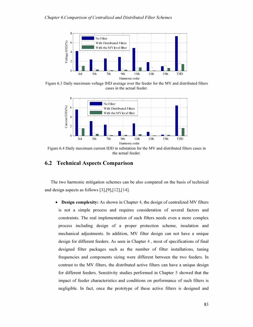
Chapter 6.Comparison of Centralized and Distributed Filter Schemes
83
3rd 5th 7th 9th 11th 13th 15th THD
0
2
4
6
8
Volt
ag
e I
HD
(%)
Harmonic order
No Filter
With Distributed Filters
With the MV level filter
Figure 6.3 Daily maximum voltage IHD average over the feeder for the MV and distributed filters
cases in the actual feeder.
3rd 5th 7th 9th 11th 13th 15th TDD
0
2
4
6
8
Curr
en
t ID
D(%
)
Harmonic order
No Filter
With Distributed Filters
With the MV level filter
Figure 6.4 Daily maximum current IDD in substation for the MV and distributed filters cases in
the actual feeder.
6.2 Technical Aspects Comparison
The two harmonic mitigation schemes can be also compared on the basis of technical
and design aspects as follows [3], [9], [12], [14].
• Design complexity: As shown in Chapter 4, the design of centralized MV filters
is not a simple process and requires consideration of several factors and
constraints. The real implementation of such filters needs even a more complex
process including design of a proper protection scheme, insulation and
mechanical adjustments. In addition, MV filter design can not have a unique
design for different feeders. As seen in Chapter 4 , most of specifications of final
designed filter packages such as the number of filter installations, tuning
frequencies and components sizing were different between the two feeders. In
contrast to the MV filters, the distributed active filters can have a unique design
for different feeders. Sensitivity studies performed in Chapter 5 showed that the
impact of feeder characteristics and conditions on performance of such filters is
negligible. In fact, once the prototype of these active filters is designed and

Chapter 6.Comparison of Centralized and Distributed Filter Schemes
84
manufactured, several of them could be installed in different residential feeders
and there is no need to conduct a study or to carry a design for each individual
system. The more number of installed filters, the more effective the system-wide
harmonic mitigation will be.
• Parallel resonance with system: The MV filters are always prone to establish a
parallel resonance with the system leading to severe harmonic amplifications.
Although, a careful design can avoid this negative impact, such issues can emerge
later because of filter detuning due to its components aging and possible changes
in the system conditions. The distributed active filters never lead to this type of
problems. Studies in Chapter 5 showed that for the actual feeder and for the low
percentages of filtering, some unexpected harmonic amplifications may be
observed for this scheme, but the impact was insignificant and just limited to filter
installation percentages less than 10%.
• System reactive power and voltage profile consideration: While this issue
must be considered in the design of MV passive filters, the distributed active filter
does not affect the fundamental frequency load flow at all.
• Changing of System conditions: In case of a feeder reconfiguration, system
extension or addition of loads, the performance of MV filters can be significantly
affected. On the other hand, as one of the advantages of distributed filters, their
operation is not dependent on the primary feeder conditions and can maintain an
effective operation regardless of the changes in the primary system. In fact, as
discussed in Chapter 5, the equivalent impedance of the primary feeder, when
transferred to the secondary system, is very negligible and does not affect the
performance of distributed filters significantly.
• Reliability: Overall, the distributed active filters provide a more reliable
harmonic mitigation scheme. Outage of a single filter branch in a centralized MV
filter may cause loss of mitigation performance or overloading of other branches.
However, outage of one or two devices in the distributed scheme does not have a
significant impact on the overall mitigation effectiveness.
• The only challenging issue about the proposed distributed active filters is the
requirements imposed on it to exhibit a low impedance. As discussed in Chapter 5,

Chapter 6.Comparison of Centralized and Distributed Filter Schemes
85
the control loop of such filters can be adjusted to comply with such impedance
requirements. However, some issues may arise regarding the operation and
control of the converter inside the device. Once the necessary power-electronic
studies on this topic are conducted and a real prototype of the device is
implemented, there will be no concern regarding this issue for using a distributed
active filter scheme for system-wide harmonic mitigation.
The above technical discussions to compare the two schemes can be summarized in
Table 6.2.
Table 6.2 Technical comparison between the two harmonic filter schemes.
Centralized MV passive
filters Distributed active filters
Less complex design
Unique design for every systems
Avoiding parallel resonance
Unnecessity of system reactive power and voltage
profile considerations
Performance in changed system conditions
Reliability
Unnecessity of further research for prototype design
6.3 Economic Analysis
This section analyzes and compares the overall costs of the two studied filter schemes.
For estimating the cost of MV filters, the data from [9], [39] is used. Since the data
belongs to the year of 1999, an annual inflation rate of 2.5% is also considered to obtain
an up-to-date cost estimation. Table 6.3 and Table 6.4 show the approximate expenses
associated with an MV filter component and installation, respectively.
The price of transformers is also assumed as given in Table 6.5 based on the data
provided by a utility company in Edmonton, Canada.
Table 6.3 Cost of capacitors and inductors for a MV filter.
Capacitor (25kV) $40 per kvar
~$2800 per phase for 10mH<L<30mH
~$3400 per phase for 30mH<L<50mH Inductor (25kV)
~$3800 per phase for 50mH<L<80mH

Chapter 6.Comparison of Centralized and Distributed Filter Schemes
86
Table 6.4 Estimated costs for each MV filter installation.
Switching Device $34,000
Overvoltage Protection $7,000
Civil $7,000
Engineering & Design $28,000
Labor Cost a $28,800
Real State $100,000
Total Installation Cost $204,800 a Labor cost is based on: 3 persons * 8 hour/day * 60 days * $20/hour.
Table 6.5 Estimated price of transformers (for the ZS filters).
Transformer size (kVA) Transformer price
Filter of actual feeder 500 $21,600
Filter of ideal feeder 2500 $30,000
By the above set of information, the overall cost of designed MV filter packages is
estimated as presented in details in Table 6.6. The price of the low-voltage capacitors of
the ZS filters are excluded in expense estimation of MV filters.
Table 6.6 Overall estimated cost for components and installations of designed MV filter packages.
For actual
feeder For ideal feeder
Single-tuned Branches
$115,200 $150,000 Components Cost
ZS Filter $21,600 $30,000
Installation Cost $204,800 $204,800
Total Cost Per Each Filter Package
$341,600 $384,800
Total Cost $683,200 $384,800
For the distributed active filters, however, the price estimation can be challenging
since there is no low-voltage single-phase virtual-impedance active filter in the present
market. However, the price of available conventional low-voltage single-phase active
filters ranges from $50 to $200. For this economic analysis, each active filter device price
is assumed $500 as a conservative estimate. Once one of such filters with a final design
in compliance with requirements specified for the proposed distributed filters (as
described in Chapter 5) is manufactured, the accurate price will be exactly known. An
average installation expense of $1500 per each device is also assumed. Hence, the total
cost of each active device filter will be $2000. The overall cost of the distributed active
filters scheme can be simply obtained by multiplying price of each device by the total
number of required devices (See Table 5.5 for the final specification of the distributed
active filters).

Chapter 6.Comparison of Centralized and Distributed Filter Schemes
87
Finally, Table 6.7 gives the total estimated costs for comparing the two harmonic filter
schemes. For both the feeders, the distributed active filter scheme is found to be the more
economic option by being less expensive than its counterpart.
Table 6.7 Comparison of total mitigation costs by the MV filters and the distributed active filters.
Total harmonic mitigation cost MV filters Distributed active filters
For actual feeder $683,200 $354,000
For ideal feeder $384,800 $316,000
6.4 Summary
This chapter presented a comprehensive comparison between the centralized passive
filter and the distributed active filter schemes. Despite the fact that both strategies can
accomplish an effective system-wide harmonic mitigation, the investigations revealed
that the distributed active filter can be a very promising option considering both
economic and technical aspects.

Chapter 7. Comparison of Centralized and Distributed Filter Schemes
88
Chapter 7
Conclusions and Future Work
7.1 Thesis Conclusions and Contributions
This thesis discussed the mitigation of harmonics in residential distribution systems. The
existing mitigation measures are not always effective in managing the new harmonic
situation, which includes several small and dispersed harmonic sources. An extensive set
of studies was conducted to propose and assess different methods to effectively mitigate
the harmonics injected by the residential loads in a distribution system. All the discussed
mitigation strategies were evaluated by performing simulation studies on a generic feeder
and a real distribution system serving residential customers in Edmonton, Canada. The
key conclusions and contributions of this thesis can be summarized as follows.
• A novel double-tuned version of transformer-based filters was proposed to
mitigate the Zero-Sequence (ZS) harmonics in a residential power system. The
double-tuned feature was revealed to be very effective for solving ZS harmonic-
caused problems such as telephone interference. Effective guidelines and
methods were developed for loading assessment and the sizing of the filters’
components. These filters’ application issues specific to mitigating telephone
interference problems were also investigated.
• An effective passive harmonic filter package including the proposed ZS filters
was introduced to accomplish a system-wide harmonic suppression. A simple
design guideline was developed by taking into account the essential
considerations for applying MV passive filters to mitigate the residential
harmonic sources of a dispersed and random nature.
• As a novel system-wide harmonic mitigation strategy, the concept of low-
voltage distributed filters was also introduced in this thesis. The scheme was
based on installing low-voltage virtual-impedance active filters in the secondary
levels of the residential distribution systems. This scheme’s design, installation

Chapter 7. Comparison of Centralized and Distributed Filter Schemes
89
and performance issues were thoroughly investigated by both developing
essential theoretical principles and performing different simulation studies. Our
method was found to be very promising for harmonic elimination in the modern
residential feeders. The results revealed that an acceptable widespread harmonic
suppression was obtained by equipping only 35% of the feeder’s service
transformers with filters.
• The thesis also performed a comprehensive comparison of the centralized and
distributed filtering options. The studies revealed that passive filters were the
proper type for the centralized scheme, while the virtual-impedance active filters
were a better choice for the distributed scheme. Both the technical and economic
aspects were considered to compare these two methods. Compared to the
centralized option, the proposed distributed active filter strategy exhibited several
merits such as being more economical and reliable and allowing for a unique
design for different feeders. As a result, this novel scheme is a very promising
and effective solution to the increasing harmonic problems in residential feeders.
7.2 Suggestions for Future Work
The author’s suggestions for continuing the studies on harmonic mitigation in residential
power distribution systems are as follows.
• As discussed in Chapter 2, a comprehensive standard which specifically
addresses the harmonic mitigation requirements in residential distribution systems
has not been developed yet. The appropriate standards and limits must be
precisely determined by the utilities by compromising between the mitigation
costs and the severity of the problems caused by the harmonics.
• In Chapter 3, the proposed ZS filters’ application for telephone interference
problems was thoroughly studied. Such filters can be also employed to mitigate
other problems caused by ZS harmonics, such as neutral current/voltage rise. If
necessary, a triplen-tuned version of such filters could be developed to trap all the
3rd, 9th and 15th harmonics.
• As explained in Chapter 5, in order to guarantee the effectiveness of distributed
active filters, they must be able to exhibit a low enough harmonic impedance.

Chapter 7. Comparison of Centralized and Distributed Filter Schemes
90
However, if the equivalent impedance of such devices be lowered too much, some
control and operational problems may occur in their converters. The possible
issues and the related concerns need to be fully investigated in the continuation of
this research. Additionally, the simple power-electronic structure of these devices
could be expanded to provide some smart applications in addition to harmonic
mitigation. Therefore, the devices could be applied to serve as a part of future
smart grid technologies as well.
• A conservative cost estimate was made for the distributed filters scheme in
Chapter 6 (including both the device and installation prices). After the active
filters have been developed and manufactured, their actual price might be lower
than our estimate. When an industrial prototype of these devices has been
implemented, a more precise estimation of the total cost can be obtained.
References
91
References
[1] J. Arrillaga, R. W. Neville, Power System Harmonics, 2nd ed., John Wiley &
Sons, 2003
[2] "IEEE Recommended Practices and Requirements for Harmonic Control in
Electrical Power Systems," IEEE Std 519-1992 , vol., no., pp.0_1, 1993
[3] "IEEE Guide for Application and Specification of Harmonic Filters," IEEE Std
1531-2003 , vol., no., pp.0_1-60, 2003
[4] D. J. Pileggi, E. M. Gulachenski, C. E. Root, T. J. Gentile, A. E. Emanuel, “The
Effect of Modern Compact Fluorescent Lights on Voltage Distortion”, IEEE
Transactions on Power Delivery, vol. 8, no. 3, July 1993, pp. 1451-1459
[5] R. Dwyer, A. K. Khan, M. McGranaghan, L. Tang, R. K. McCluskey, R. Sung, T.
Houy, “Evaluation of Harmonic Impacts from Compact Fluorescent Lights on
Distribution Systems”, IEEE Transactions on Power Systems, vol. 10, no. 4, Nov.
1995, pp. 1772-1779
[6] D. Salles, C. Jiang, , W. Xu, W. Freitas and H. Mazin,“Assessing the Collective
Harmonic Impact of Modern Residential Loads – Part I: Method”, , IEEE
Transactions on Power Delivery , vol.27, no.4, pp.1937-1946, Oct. 2012
[7] C. Jiang, D. Salles, W. Xu and W. Freitas, “Assessing the Collective Harmonic
Impact of Modern Residential Loads – Part II: Applications” , Accepted to
publish in IEEE Transactions on Power Delivery
[8] Nassif, A.B.; Wilsun Xu; Freitas, W.; , "An Investigation on the Selection of
Filter Topologies for Passive Filter Applications," IEEE Transactions on Power
Delivery , vol.24, no.3, pp.1710-1718, July 2009
[9] D. Bohaichuk, C. Muskens, W. Xu, “Mitigation of Harmonics in Oil Field
Electric Systems Using a Centralized Medium Voltage Filter”, presented at the
9th IEEE ICHQP, Oct. 2000, pp. 614-618
[10] C. J. Chou, C. W. Liu, J. Y. Lee, “Optimal Planning of Large Passive-Harmonic-
Filters Set at High Voltage Level”, IEEE Transactions on Power Systems, vol. 15,
no. 1, pp. 433-441, Feb. 2000
[11] Gonzalez, A. Damian, McCall, C. John , "Design of Filters to Reduce Harmonic
Distortion in Industrial Power Systems," IEEE Transactions on Industry
Applications, vol.IA-23, no.3, pp.504-511, May 1987

References
92
[12] J.C. Das, "Passive filters - potentialities and limitations," IEEE Transactions on
Industry Applications , vol.40, no.1, pp. 232- 241, Jan.-Feb. 2004
[13] H.L. Ginn, III; L.S. Czarnecki; , "An optimization based method for selection of
resonant harmonic filter branch parameters," IEEE Transactions on Power
Delivery , vol.21, no.3, pp.1445-1451, July 2006.
[14] T.H. Ortmeyer, T. Hiyama , "Distribution system harmonic filter planning,"
IEEE Transactions on Power Delivery, vol.11, no.4, pp.2005-2012, Oct 1996.
[15] Chang, G.W.; Hung-Lu Wang; Shou-Yung Chu; , "Strategic placement and
sizing of passive filters in a power system for controlling voltage distortion,"
IEEE Transactions on Power Delivery , vol.19, no.3, pp. 1204- 1211, July 2004.
[16] Mau Teng Au; Jovica V. Milanovic; , "Planning Approaches for the Strategic
Placement of Passive Harmonic Filters in Radial Distribution Networks," IEEE
Transactions on Power Delivery , vol.22, no.1, pp.347-353, Jan. 2007.
[17] Chang, G.W.; Shou-Yung Chu; Hung-Lu Wang; , "Sensitivity-based approach
for passive harmonic filter planning in a power system," Power Engineering
Society Winter Meeting, 2002. IEEE , vol.2, no., pp. 937- 940 vol.2, 2002
[18] Chi-Jui Wu; Jung-Chen Chiang; Shih-Song Yen; Ching-Jung Liao; Jin-Shyr
Yang; Tzong-Yih Guo; , "Investigation and mitigation of harmonic amplification
problems caused by single-tuned filters," IEEE Transactions on Power Delivery,
vol.13, no.3, pp.800-806, Jul 1998.
[19] Akagi, H.; , "New trends in active filters for power conditioning,", IEEE
Transactions on Industry Applications , vol.32, no.6, pp.1312-1322, Nov/Dec
1996.
[20] Singh, B.; Al-Haddad, K.; Chandra, A.; , "A review of active filters for power
quality improvement," IEEE Transactions on Industrial Electronics , vol.46,
no.5, pp.960-971, Oct 1999
[21] T.Q., Tran; L.E., Conrad; Stallman, B.K.; , "Electric shock and elevated EMF
levels due to triplen harmonics," IEEE Transactions on Power Delivery, vol.11,
no.2, pp.1041-1049, Apr 1996
[22] T.M., Gruzs; "A survey of neutral currents in three-phase computer power
systems ,", Conference Record., Industrial and Commercial Power Systems
Technical Conference, vol., no., pp.114-122, 7-11 May 1989

References
93
[23] "IV.B. Power Line Harmonic Effects on Communication Line Interference IEEE
Working Group on Power System Harmonics," Power Engineering Review,
IEEE , vol.PER-5, no.9, pp.56, Sept. 1985.
[24] W. Jewell, W. Miller, T. Casey, "Audible telephone noise from small harmonic
sources on single-phase distribution," Harmonics And Quality of Power, 1998.
Proceedings. 8th International Conference on , vol.2, no., pp.890-895 vol.2, 14-
18 Oct 1998
[25] IEEE Working Group on Nonsinusoidal Situations: Effects on Meter
Performance and Definitions of Power, “Practical Definitions for Powers in
Systems with Nonsinusoidal Waveforms and Unbalanced Loads: a Discussion”,
IEEE Transactions on Power Delivery, vol. 11, no. 1, January 1996, pp. 79-101.
[26] "IV.B. Power Line Harmonic Effects on Communication Line Interference IEEE
Working Group on Power System Harmonics," Power Engineering Review,
IEEE , vol.PER-5, no.9, pp.56, Sept. 1985
[27] Ch. Jiang, “A Probabilistic Bottom-up Approach for Modeling and Simulation of
Residential Distributed Harmonic Sources”, MSc. thesis, University of Alberta,
Canada, 2012.
[28] A. Wang, “Harmonic Impact of Modern Residential Loads on Distribution Power
System and Mitigation Solutions”, MSc. thesis, University of Alberta, Canada,
2011
[29] W. Xu, J. R. Marti, and H. W. Dommel , "A multiphase harmonic load flow
solution technique," IEEE Transactions on Power Systems, vol.6, no.1,pp.174-
182, Feb 1991
[30] IEC Standard 1000-3-6, “Assessment of Emission Limits for Distorting loads in
MV and HV Power Systems – Basic EMC Publication”, 1996
[31] W. Xu , V. Sharma “Evaluation of the Use of Zero Sequence Harmonic Traps in
Commercial Buildings”, CEA Project Report 311-D-937, 1998
[32] P., Rodriguez;I., Candela; S., Bogarra; R.,Teodorescu ; F., Blaabjerg; ,
"Cancellation of neutral current harmonics by using a four-branch star hybrid
filter," Power Electronics Specialists Conference, 2008. PESC 2008. IEEE , vol.,
no., pp.1041-1047, 15-19 June
[33] "Passive power filter tunable at two simultaneous frequencies, one for zero-
sequence and another on for positive-sequence (in Spanish)", Spanish patent, Jan.
2007

References
94
[34] W. Jewell, W.L. Miller, T. Casey , "Filtering dispersed harmonic sources on
distribution," IEEE Transactions on Power Delivery, vol.15, no.3, pp.1045-1051,
Jul 2000
[35] H. Jou; J. Wu; K. Wu; W. Chiang; Y. Chen; , "Analysis of zig-zag transformer
applying in the three-phase four-wire distribution power system,", IEEE
Transactions on Power Delivery , vol.20, no.2, pp. 1168- 1173, April 2005
[36] E. Larsen, “Filter for removing harmonic current from a neutral conductor”, U.S.
patent 5914540, Jun. 22, 1999
[37] "IEEE Standard for Shunt Power Capacitors," IEEE Std. 18-2002 (Revision of
IEEE Std 18-1992) , vol., no., pp.0_1-17, 2002
[38] "IEEE Recommended Practice for Inductive Coordination of Electric Supply and
Communication Lines," IEEE Std 776-1992 , vol., no., pp.1-64, Feb. 8 2012
[39] W.Xu, "Assessment of Harmonic Filtering Options", A research report submitted
to ATCO Electric Ltd., June 1999
[40] Po-Tai Cheng; Tzung-Lin Lee; , "Distributed Active Filter Systems (DAFSs): A
New Approach to Power System Harmonics,", IEEE Transactions on Industry
Applications , vol.42, no.5, pp.1301-1309, Sept.-Oct. 2006.
[41] Tzung-Lin Lee; Po-Tai Cheng; Akagi, H.; Fujita, H.; , "A Dynamic Tuning
Method for Distributed Active Filter Systems,", IEEE Transactions on Industry
Applications , vol.44, no.2, pp.612-623, March-april 2008.
[42] Tostes, M.Ed.L.; Bezerra, U.H.; Silva, R.D.S.; Valente, J.A.L.; de Moura,
C.C.M.; Branco, T.M.M.; , "Impacts over the distribution grid from the adoption
of distributed harmonic filters on low-voltage customers," IEEE Transactions on
Power Delivery, vol.20, no.1, pp. 384- 389, Jan 2005.
[43] Akagi, H.; Fujita, H.; Wada, K.; , "A shunt active filter based on voltage
detection for harmonic termination of a radial power distribution line,", IEEE
Transactions on Industry Applications , vol.35, no.3, pp.638-645, May/Jun 1999.
[44] Ryckaert,W.;Ghijselen, J.;Desmet, J.;Van den Bossche, A.;Melkebeek, J.;Van de
Sype, D.;, "The location of a resistive shunt harmonic impedance along a
distribution feeder and its influence on harmonic propagation," Electrical
Engineering, Springer Berlin, Vol. 87, Issue 6, Oct 2005.
[45] T .A. Short, Electric Power Distribution Handbook CRC Press 2003

References
95
[46] J.M. Frank, (1994) Origin, development and design of K-factor transformers,
Conference Record, IEEE Industry Applications Society Annual Meeting, Denver,
pp. 2273–4
[47] R.D. Henderson and P.J. Rose. Harmonics: the Effects on Power Quality and
Transformers., IEEE Transactions on Industry Applications, vol.30, no.3,
May/June, 1994, pp.528-532
[48] "IEEE Recommended Practice for Establishing Liquid-Filled and Dry-Type
Power and Distribution Transformer Capability When Supplying Nonsinusoidal
Load Currents," IEEE Std C57.110-2008 (Revision of IEEE Std C57.110-1998) ,
vol., no., pp.c1-44, Aug. 15 2008
[49] D. E. Rice. “Adjustable Speed Drive and Power Rectifier Harmonics-Their
Effects on Power Systems Components.” IEEE Transactions on Industry
Applications, vol.22, no.1, Jan/Feb., 1986, pp.161-177

Appendix
96
Appendix
Appendix A Aggregated harmonic model of secondary systems
This section of appendix explains how the equivalent aggregated harmonic models of the
secondary systems are established. The procedure is similar as in [28], however, the
proposed distributed active filters are also included in the models. Section A.1 describes
the modeling procedure where the distributed filters are included as well. Next, the
developed aggregated model will be verified by simulations for a typical secondary
system in section A.2.
A.1 Modeling procedure
In order to cover all the studies of this thesis, the aggregated model must be derived for
three scenarios (Figure A.1): 1) the service transformer is supplying the houses without
any filter 2) when a filter is attached to the service transformer and 3) the case when filter
is installed at one of the houses. As the first step, the equivalent circuits for the three
scenarios are established as shown in Figure A.2 (a)-(c). In the equivalent circuits, the
conductors connecting the houses other than the house with filter are ignored since of
their negligible effect on the harmonic flows. However, for the third scenario, the
secondary conductor and service conductor of the filter house do have the impact on
harmonic flow and are included as shown in Figure A.2 (c). When generating the
aggregated models for the whole feeder, lengths of these conductors (Lsec and Lserv in
Figure A.1) for each secondary system are randomly chosen from typical ranges as the
followings,
Lsec: 20m-60m,
Lserv: 5m-25m.

Appendix
97
Figure A.1 A general secondary system with (or without) the distributed filters installed at either
the service transformer or the closest house.
(a) (b)
(c)
Figure A.2 Equivalent circuit of the system (a) without any filter (b) with a filter installed at the service transformer (c) with a filter installed at the closest house
Once the equivalent circuits are established, their Y and I matrix can be developed and
reduced to obtain the final simplified models. The equivalent reduced Y and I matrices
will only include nodes P and N where the secondary system is connected to the primary
feeder through the service transformer (The procedure is thoroughly described in [28] for
the first scenario). Finally, each of developed simplified models for each secondary
system looks like the circuit shown in Figure A.3.
Figure A.3 The developed aggregated harmonic model of a secondary distribution system

Appendix
98
A.2 Aggregated model verification
The developed simplified model for all the three scenarios (No filter, filter at service
transformer and filter at the closest house) is verified by performing two sets of harmonic
load flows on a typical secondary system. The first scenario is obtained by using the
comprehensive simulation circuit explained in section 5.3 and the other scenario is
performed by employing the developed model as shown in Figure A.4.
Figure A.4 Circuit for verification of the developed aggregated model
The results of the two harmonic flow studies (model versus detailed simulation) are
shown and compared through Figure A.5 and Figure A.6 by plotting the harmonic current
distortion profile of the current entering the primary side (Ih in Figure A.1 and Figure
A.4).
The results obtained by the model and the simulation match very well, so that the
developed models are quite effective in representing the service transformers and their
supplied residential loads for studying both the distributed filters and also other
mitigation schemes in a primary distribution system.
1 3 5 7 9 11 13 15 17 19 21 230
1
2
3
4
5
6
Time(hour)
TDDI(%
)
NoFilter-Model
NoFilter-Simulation
Filter at service transformer-Model
Filter at service transformer-Simulation
Filter at the closest house-Model
Filter at the closest house-Simulation
Figure A.5 Current TDD daily profile of the different cases obtained by the simplified model and detailed simulation

Appendix
99
3rd 5th 7th 9th 11th 13th 15th TDD0
0.5
1
1.5
2
2.5
Dai
ly A
vera
ge C
urr
en
t ID
D(%
)
Harmonic order
NoFilter-Model
NoFilter-Simulation
Filter at service transformer-Model
Filter at service transformer-Simulation
Filter at the closest house-Model
Filter at the closest house-Simulation
Figure A.6 Daily average current IDD of the different cases obtained by the simplified model and detailed simulation
Appendix B Loading Assessment of the ZS Filter Transformer
In general, the literature presents two categories of methods for the loading evaluation of
transformers exposed to high harmonic currents:
• One approach is to calculate the k-factor index based on the harmonic content of the
operation current. Next, a specialized k-factor type transformer able to operate under such
a harmonic level is selected for that application [46]- [48].
• The other method is to calculate the maximum allowed current based on the
harmonic content flowing in the transformer and to operate it under a decreased load to
avoid overheating [1], [48].
However, the intention of assessing the loading of the transformer inside a ZS filter is
neither to use a specialized transformer (k-factor) nor to decrease the transformer current.
In fact, the main objective is to verify that the transformer of a selected size is not
overheated by the harmonics flowing inside the filter. For this thesis, the proper
transformer loading assessment method for the design of ZS filters is developed based on
the same theories behind the k-factor and transformer derating methods in the IEEE std.
( [48]).
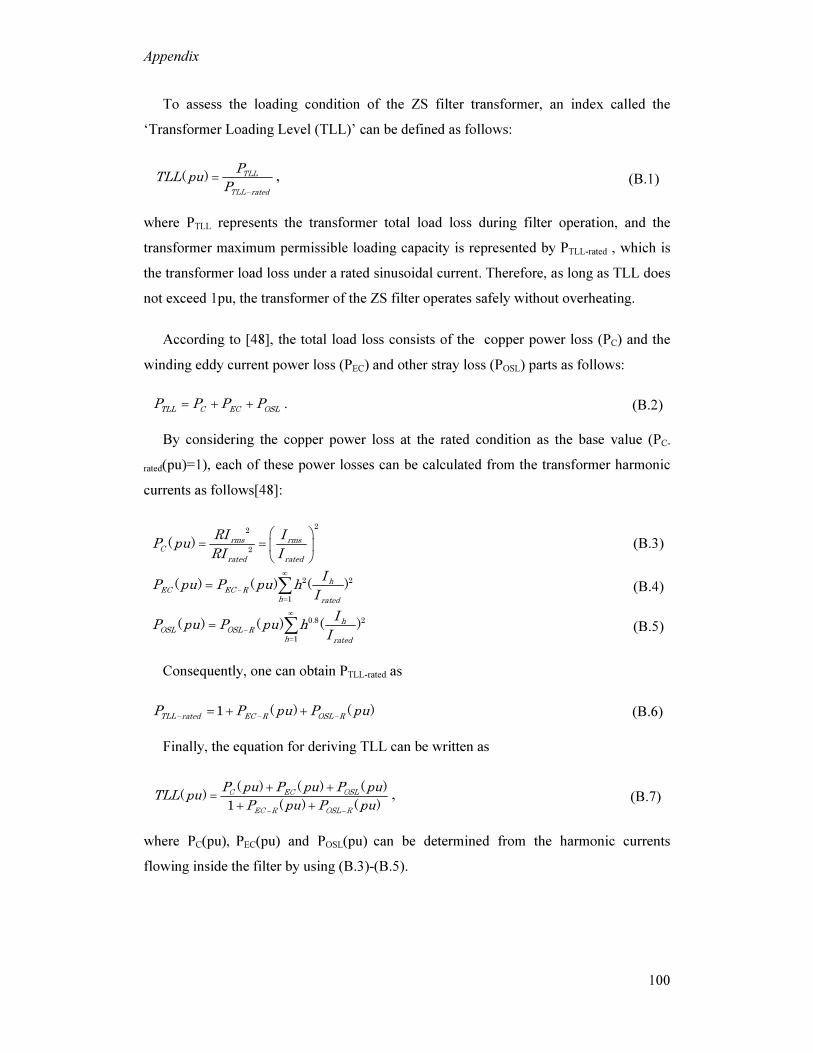
Appendix
100
To assess the loading condition of the ZS filter transformer, an index called the
‘Transformer Loading Level (TLL)’ can be defined as follows:
( ) TLL
TLL rated
PTLL pu
P−
= , (B.1)
where PTLL represents the transformer total load loss during filter operation, and the
transformer maximum permissible loading capacity is represented by PTLL-rated , which is
the transformer load loss under a rated sinusoidal current. Therefore, as long as TLL does
not exceed 1pu, the transformer of the ZS filter operates safely without overheating.
According to [48], the total load loss consists of the copper power loss (PC) and the
winding eddy current power loss (PEC) and other stray loss (POSL) parts as follows:
TLL C EC OSLP P P P= + + . (B.2)
By considering the copper power loss at the rated condition as the base value (PC-
rated(pu)=1), each of these power losses can be calculated from the transformer harmonic
currents as follows [48]:
22
2( ) rms rms
C
rated rated
RI IP pu
RI I
= =
(B.3)
2 2
1
( ) ( ) ( )h
EC EC R
h rated
IP pu P pu h
I
∞
−
=
= ∑ (B.4)
0.8 2
1
( ) ( ) ( )h
OSL OSL R
h rated
IP pu P pu h
I
∞
−
=
= ∑ (B.5)
Consequently, one can obtain PTLL-rated as
1 ( ) ( )TLL rated EC R OSL R
P P pu P pu− − −
= + + (B.6)
Finally, the equation for deriving TLL can be written as
( ) ( ) ( )( )
1 ( ) ( )C EC OSL
EC R OSL R
P pu P pu P puTLL pu
P pu P pu− −
+ +=
+ +
, (B.7)
where PC(pu), PEC(pu) and POSL(pu) can be determined from the harmonic currents
flowing inside the filter by using (B.3)-(B.5).

Appendix
101
The index calculation also requires the PEC-R(pu) (‘Eddy current loss factor’) and
POSL-R(pu) (‘Other stray loss factor’) values, which are, in fact, constant coefficients
dependent mainly on the transformer design, size and structure.
According to the recommendation of IEEE standard, POSL-R(pu) can be obtained from
PEC-R(pu) by following a simple rule of thumb [48]:
( ) ( )OSL R EC R
P pu P puα− −
= , (B.8)
where α is approximately 2 for a liquid-filled transformer and 0.5 for a dry-type
transformer. According to this estimation, the only unknown in the TLL definition is PEC-
R(pu). In general, no practical and simple method to obtain this value from the
transformer nameplate is available [48], [49]. The typical values of the eddy current loss
factor for some different types of transformers are shown in Table B.1 [49].
Table B.1 Typical values of ‘Eddy current loss factor’ (PEC-R) [49]
Equipment PEC-R(%)
≤1000 kVA 3-8 Dry Type Transformers
≥1500 kVA 12-20
≤2500 kVA 1
2500~5000 kVA 1-5 Oil-Filled Type Transformers
> 5000 kVA 9-15
For the loading assessment analysis in this thesis, a conservative value of PEC-R(pu)
was chosen according to the above table.
Appendix C MV passive harmonic filter design details
C.1 Design of single-tuned filter branches
Figure C.1 shows schematic of a conventional single-tuned filter branch. As discussed
in Chapter 4, this filter is a part of the proposed filter package and its capacitors are sized
according to the iterative design procedure.

Appendix
102
Figure C.1. A conventional single-tuned filter branch.
Once the capacitor size is known, the inductor size can be calculated by the following
equation.
2 2
0
1
(2 )t
LCh fπ= (C . 1)
where f0 is the power frequency (f0=60Hz in North America) and ht the tuned
harmonic frequency. Based on the general practice, the filter is not tuned to exact
harmonic frequencies but to a slightly lower frequency to avoid the following issues [3].
a) Capacitors with metalized film construction lose capacitance as they age which
may result in slight increases in tuning frequency when used in harmonic filters.
Therefore, a single-tuned filter tuned at below its rated frequency can still perform
acceptable filtering even after the capacitor aging.
b) Tuning a harmonic filter too sharply to the harmonic frequency can unnecessarily
stress the components and consequently increases prone of overloading.
c) The manufacturing tolerance of the inductors can cause a resulted tuning frequency
higher than its designed nominal value.
d) Operation of capacitor fuses on failed capacitor elements or units can result in
slightly boosting the tuning frequencies.
For example, in this thesis, single-tuned filters for 5th and 7th harmonics are tuned to
4.9 and 6.9 harmonic orders respectively.

Appendix
103
Appendix D Distributed Active Filter Scheme Design Details
D.1 Analysis of a secondary system with generalized configuration
In section 5.3.2, analytical results were presented for a system with generalized
configuration to assess different filter placement options. This section of appendix
describes the analytical procedure used to estimate the filter effectiveness, when it is
installed at locations A or B of the system (see Figure 5.17).
For location A, the system can be easily analyzed similarly as sections 5.2.1 and 5.2.2
of the report and by the means of equivalent circuit shown in Figure 5.9. The equations
( 5.16)-( 5.18) will be modified as below for the current case,
, ,
,,
2, 1
,
4 4 2
2
Filteredh p eq F
No filtereq F sysh p
sys eq pr T L
eq F F Lb
I Z
Z ZI
Z Z Z Z
Z Z Z
α
=
+ = + +
= +
, (D . 1)
where ZL1 and ZLb are the impedances of the first secondary conductor and the filter
house service conductor respectively. Other variables are still as the same as defined in
the report.
However, a more sophisticated analysis is needed for the filter performance when it is
installed in location B. The equivalent circuit shown in Figure D.1 is used to analyze this
situation. In this circuit, ZL1 and ZL2 are the impedances of the first and second secondary
conductors where ZLb represents the impedance of the service conductor connecting the
house with filter. Ih,A1 and Ih,B1 represent the harmonic currents generated by the first
group of houses and Ih,A2 and Ih,B2 are associated with the second groups of houses,
respectively.

Appendix
104
",h pI : :1 α α
, 1h AI
, 1h BI
, 2h AI
, 2h BI
Figure D.1 The equivalent circuit for the case of placing the filter in location A of the generalized
system shown in Figure 5.17.
According to the superposition principle and analyses conducted in sections 5.2.1 and
5.2.2, the primary harmonic current can be derived as below,
, 2 ,, , 1 , 1 , 2 , 2
, 2 1 , 2 1
2( ) ( )
2 2 2 2
eq F L eq FFilteredh p h A h B h A h B
eq F L L sys eq F L L sys
Z Z ZI I I I I
Z Z Z Z Z Z Z Zα α
+
= + + +
+ + + + + +
(D . 2)
where 2
,
,
4 4
2
sys eq pr T
eq F F Lb
Z Z Z
Z Z Z
α = +
= +
(D . 3)
And when there is no filter in the system, one have the below equation similarly as
( 5.3),
, , 1 , 1 , 2 , 2( )NoFilterh p h A h B h A h BI I I I Iα= + + + (D . 4)
In order to simplify the derived equations, harmonic currents generated by each group
of houses can be assumed proportional to the number of houses,
1, 1 , 2
2
1, 1 , 2
2
h A h A
h B h B
NI I
N
NI I
N
≈
≈
(D . 5)
By dividing (D . 2) over (D . 4) and substituting (D . 5) into them,
1, 2
, 1 2
, 2 1,
2
2 2
Filtered eq F Lh p
NoFiltereq F L L sysh p
NZ Z
I N N
Z Z Z ZI
+
+
≈
+ + +
(D . 6)
Finally, the above equation is employed to estimate the filter performance at
location B and obtaining the analytical results (associated with generalized configuration)
presented in section 5.3.2 of the thesis.

Appendix
105
D.2 Impact of feeder shunt capacitance on distributed filters performance
By the results presented in section 5.4.1 of the thesis, shunt capacitance of underground
cables inside the actual feeder were found to make the distributed filters somehow
ineffective when the percentage of equipped transformers with the filters were lower than
10%. Theoretical explanation for such phenomenon is presented in this appendix.
Shunt capacitances can always cause abnormalities in system harmonic load flow by
participating in parallel resonances with inductance of other system components. Figure
D.2 shows a simplified system schematic to investigate any possible interaction of the
distributed filters installed in secondary systems with primary power-lines shunt
capacitance.
Sub
F
Underground
conductor
Service
transformer
Figure D.2 A simplified schematic of feeder to analyze possible interactions of distributed filters and power-lines shunt capacitance.
The equivalent circuit for the case of no filter is shown in Figure D.3(a). As observed
in the normal situation, because of the loads high impedance, there is no inductor branch
in the system to establish a parallel resonance with the shunt capacitances. However,
when a distributed filter is installed as shown in the circuit of Figure D.3(b), its low
impedance bypasses the loads impedance providing a path for the transformer leakage
inductance to establish a parallel resonance with the shunt capacitance of the
underground cables.
(a) (b)
Figure D.3 The equivalent circuits showing how a parallel resonance may be established with installing the distributed filters.

Appendix
106
Fortunately, based on the report results this phenomenon is unlikely to cause a
significant problem for the proposed filter scheme and is only observed for the actual
feeder (including long underground cables) and just in the low percentages of filters
installation less than 10%.
D.3 Filter Impedance study for the closest house location
This appendix presents the primary system simulation results for the sensitivity of
distributed filters to the filter impedance value, where the filters are installed in the
closest house to their supplying transformer. As mentioned in section 5.4.3, the results do
not differ from the case of direct connection to service transformers considerably.
0 0.5 1 1.5 20
20
40
60
80
100
Filter Impedance (Ω)
Per
centa
ge
decr
ease
of
TD
DI(%
)
75%50%
25%
100%
0 0.5 1 1.5 20
20
40
60
80
100
Filter Impedance (Ω)
Per
centa
ge
decr
ease
of
TH
DV(%
)
75%50%
25%
100%
(a) (b)
0 0.5 1 1.5 20
20
40
60
80
100
Filter Impedance (Ω)
Per
centa
ge
decr
ease
of
TD
DI(%
)
75%50%
25%
100%
0 0.5 1 1.5 2
0
20
40
60
80
100
Filter Impedance (Ω)
Per
centa
ge
decr
ease
of
TH
DV(%
)
75%
50%25%
100%
(c) (d)
Figure D.4. Percentage decrease of current TDD and voltage THD versus filter impedance including four different percentages of service transformers equipped with virtual-impedance distributed filters (a) (b) Ideal feeder (c)(d) Actual feeder (The filters are installed at the closest house to the service transformers).

Appendix
107
D.4 Loading Estimation of Distributed Active Filters
In this thesis, the loading of distributed filters are estimated on the basis of the feeder
harmonic currents in substation. By a conservative approach, it is assumed that the
distributed filters collectively sink the whole harmonic current of the feeder which in
normal condition flows to the substation. The average harmonic current flowing inside
each device can be derived by dividing the total current by the number of the devices.
The service transformers voltage ratio needs to be considered too.
Therefore, the expression shown below is used to estimate the filters loading.
14.4( )
240
Filter PhaseA PhaseB PhaseCh h Sub h Sub h Sub F
kVI I I I N
V− − −
= + + × ÷ , (D . 7)
where Nf is the number of filter devices and IhFilter is the average current entering each
filter. Ih-SubphaseX is also the harmonic current of each phase at the feeder substation. For
the actual feeder, the substation harmonic current is derived from both the simulation
model and also some field measurements conducted in the feeder substation.