METHODOLOGY ARTICLE Open Access Identifying structural ...

Feldman BMC Bioinformatics 2012, 13:286http://www.biomedcentral.com/1471-2105/13/286

METHODOLOGY ARTICLE Open Access

Identifying structural domains of proteinsusing clusteringHoward J Feldman

Abstract

Background: Protein structures are comprised of modular elements known as domains. These units are used andre-used over and over in nature, and usually serve some particular function in the structure. Thus it is useful to beable to break up a protein of interest into its component domains, prior to similarity searching for example.Numerous computational methods exist for doing so, but most operate only on a single protein chain and manyare limited to making a series of cuts to the sequence, while domains can and do span multiple chains.

Results: This study presents a novel clustering-based approach to domain identification, which works equally wellon individual chains or entire complexes. The method is simple and fast, taking only a few milliseconds to run, andworks by clustering either vectors representing secondary structure elements, or buried alpha-carbon positions,using average-linkage clustering. Each resulting cluster corresponds to a domain of the structure. The method iscompetitive with others, achieving 70% agreement with SCOP on a large non-redundant data set, and 80% on aset more heavily weighted in multi-domain proteins on which both SCOP and CATH agree.

Conclusions: It is encouraging that a basic method such as this performs nearly as well or better than some farmore complex approaches. This suggests that protein domains are indeed for the most part simply compactregions of structure with a higher density of buried contacts within themselves than between each other. Byrepresenting the structure as a set of points or vectors in space, it allows us to break free of any artificial limitationsthat other approaches may depend upon.

Keywords: Domain assignment, Agglomerative clustering, Average-linkage, Structural domain

BackgroundIt is well understood that proteins are made up of struc-tural and functional subunits or 'domains'. Ever sincedomains were first described [1], numerous methodshave been proposed to identify domains within proteinstructures. These approaches can vary widely dependingon whether the assignments are made from sequencealone or from the 3D structure, and often involve partialor complete manual intervention. The domain identifi-cation problem is somewhat unique in structural biologyin that it is at least in some cases subjective. Differentauthors have different, though not mutually exclusive,ideas about what a domain should be - a functional unitwhich is reused over and over [2]; a segment of a struc-ture which has been conserved and reused geneticallyacross different families of proteins [3]; or simply a

Correspondence: [email protected] Computing Group, Inc., 1010 Sherbrooke St. W., Suite 910,Montreal, Quebec H3A 2R7, Canada

© 2012 Feldman; licensee BioMed Central LtdCommons Attribution License (http://creativecreproduction in any medium, provided the or

compact region of the protein where intra-atom contactsoutweigh contacts to atoms outside the domain, forrapid self-assembly [1]. Domain definitions are also sepa-rated into 'genetic domains' which may be comprised ofpieces from multiple chains, and regular ones which arecompletely contained within a single chain.As a result of these different paradigms, there still

does not exist a precise definition for a protein domain,nor do experts always agree on the number or locationof domains within a given structure. This makes itextremely difficult to come up with a fully automatedalgorithm, then, to assign domain boundaries. That said,the SCOP [4] and CATH [5] databases are typically usedfor the problem. We found that these agree only 80% ofthe time on number of domains however, over 75,500chains that they have in common (SCOP 1.75 and CATH3.4.0, data not shown)! Despite these problems, splittinga protein into domains is often desirable. For examplewhen performing homology modelling, one often seeks a

. This is an Open Access article distributed under the terms of the Creativeommons.org/licenses/by/2.0), which permits unrestricted use, distribution, andiginal work is properly cited.

mailto:[email protected]

http://creativecommons.org/licenses/by/2.0

Feldman BMC Bioinformatics 2012, 13:286 of 12http://www.biomedcentral.com/1471-2105/13/286

template to model parts of the structure from. In thiscase it makes the most sense to find and use similardomains from known structures, which may provide use-ful templates when searching for similarity to the entirechain may not. Knowledge of domain boundaries canalso be used to improve the accuracy of sequence align-ments. Many different approaches have been used to splitproteins into domains, and these can be divided intosequence-based and structure-based approaches.Sequence-based domain identification usually involves

comparing the sequence in question to a database ofprotein sequences where the domains have already beendefined (such as SCOP) using an alignment tool such asBLAST [6]. More advanced methods such as HMMER[7] make use of multiple sequence alignments of domainfamilies, such as those compiled by InterPro [3], and useHidden Markov Models (HMM) or other approaches tocompare a query sequence against them, recording hitsto the various domain families. Examples of sequence-based domain databases include PFAM [8] and SMART[9]. These methods work quite well when sequence iden-tity to known folds is medium to high (above 35% or so)but they fail on novel or unusual folds, or those withonly very distant homologs. The precise boundaries maybe off by quite a bit as well if there are large insertionsor deletions in the sequence relative to the rest of thefamily.Structure-based algorithms should in theory be simple

and straightforward, and often to the human eye it is ob-vious where domain boundaries should be drawn whenviewing a 3D structure. Nevertheless, it has proved a dif-ficult computational problem and no automated algo-rithm agrees more than about 80% of the time withSCOP or CATH assignments. A wide variety of methodsexist, some based on graph theory and contact maps,some based on secondary structure layout. Some allowonly single cuts to be made resulting in domains madeof contiguous segments only and a maximum of 3 or 4domains per chain, others do not have this restriction.PUU [10] builds a contact matrix and tries to maximizeinteractions within each unit and minimize them be-tween units, through a series of cuts to the sequence.PDP [11] also attempts to make a series of cuts tomaximize interactions but normalized the contact countby the expected number of contacts, based on surfacearea of the proposed domain. DDOMAIN [12] is alsobased on a series of recursive cuts to try to maximizeintra-domain contacts, and also employs a pairwise sta-tistical potential instead of a simple contact count whichslightly improves performance. DomainParser [13,14]uses network flow algorithms, hydrophobic moment pro-file and neural networks to produce its domain partition-ing. NCBI's VAST algorithm [15,16], though not fullydescribed anywhere, makes use of domains identified as

compact structural units within protein 3D structuresusing purely geometric criteria. DomainICA [17] usesgraph theory with secondary structure elements as thenodes and edges determined by proximity. The algo-rithm partitions the graph to maximize cycle distribu-tions, and its simplicity is appealing. dConsensus [18]provides a means for rapidly comparing assignments bythe different approaches.Despite the number of algorithms that have been

described, most of comparable performance, it seems eachhas certain disadvantages. As mentioned some methodscannot deal with domains comprised of multiple contigu-ous segments, and most cannot deal with genetic domains(those with pieces from multiple chains). Some methodsare very slow, and some cannot place boundaries midwaythrough secondary structure elements. This study investi-gates a novel, intuitive algorithm for domain identifica-tion by simply clustering α-carbon positions or secondarystructure vectors in space. It is very fast, taking underone second for all but the largest proteins, and intuitivelyobvious. By its nature it has no maximum number ofdomains it can define, nor limitation on where domainboundaries can occur. Even domains comprised of piecesfrom multiple chains, such as when domain swappingoccurs [19,20], are detected without changes to thealgorithm.

ResultsTwo distinct but related algorithms were studied, asdescribed in Methods: the α-carbon based algorithm(CA) and the secondary structure element based algo-rithm (SS). Both make use of average-linkage clusteringto produce and then cut a dendrogram; they differ onlyin the objects that they cluster. The main data set usedto optimize the algorithms was the ASTRAL30 set, con-sisting of 8792 domains in 7178 non-redundant proteinchains. Only 7076 of these chains actually still existed inthe current Protein Data Bank (PDB) however and socomprised the training set used in this study for the CAalgorithm. Only 6841 of these had sufficient secondarystructure to use the SS algorithm, so this slightly smallertraining set was used in that case. Both algorithms haveonly two adjustable parameters: the minimum value forcutting the cluster dendrogram, m, and the step size todetermine whether to make a cut, s.For the CA algorithm, a range of these values were

tested, and the performance on the training set recordedfor each of 1-, 2-, 3-, and 4-domain chains, summarizedin Table 1. An assignment was considered correct whenit agreed with SCOP, since ASTRAL is based on the SCOPdomain database. The Matthews Correlation Coefficient(MCC) was also computed, which gives a statistically lessbiased measure (compared to percentage correct) of clas-sification success given the large proportion of single

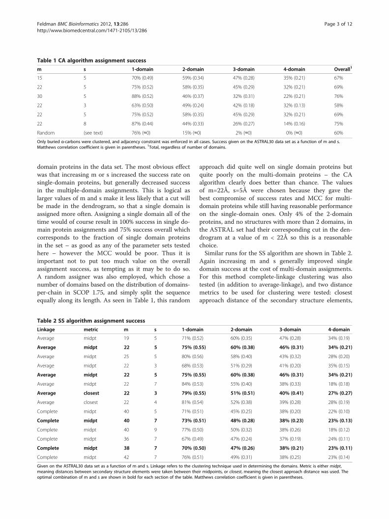
Table 1 CA algorithm assignment success

m s 1-domain 2-domain 3-domain 4-domain Overall1

15 5 70% (0.49) 59% (0.34) 47% (0.28) 35% (0.21) 67%

22 5 75% (0.52) 58% (0.35) 45% (0.29) 32% (0.21) 69%

30 5 88% (0.52) 46% (0.37) 32% (0.31) 22% (0.21) 76%

22 3 63% (0.50) 49% (0.24) 42% (0.18) 32% (0.13) 58%

22 5 75% (0.52) 58% (0.35) 45% (0.29) 32% (0.21) 69%

22 8 87% (0.44) 44% (0.33) 26% (0.27) 14% (0.16) 75%

Random (see text) 76% (≈0) 15% (≈0) 2% (≈0) 0% (≈0) 60%

Only buried α-carbons were clustered, and adjacency constraint was enforced in all cases. Success given on the ASTRAL30 data set as a function of m and s.Matthews correlation coefficient is given in parentheses. 1Total, regardless of number of domains.


domain proteins in the data set. The most obvious effectwas that increasing m or s increased the success rate onsingle-domain proteins, but generally decreased successin the multiple-domain assignments. This is logical aslarger values of m and s make it less likely that a cut willbe made in the dendrogram, so that a single domain isassigned more often. Assigning a single domain all of thetime would of course result in 100% success in single do-main protein assignments and 75% success overall whichcorresponds to the fraction of single domain proteinsin the set – as good as any of the parameter sets testedhere – however the MCC would be poor. Thus it isimportant not to put too much value on the overallassignment success, as tempting as it may be to do so.A random assigner was also employed, which chose anumber of domains based on the distribution of domains-per-chain in SCOP 1.75, and simply split the sequenceequally along its length. As seen in Table 1, this random

Table 2 SS algorithm assignment success

Linkage metric m s 1-doma

Average midpt 19 5 71% (0.5

Average midpt 22 5 75% (0



Average midpt 22 5 75% (0


Average closest 22 3 79% (0

Average closest 22 4 81% (0.5

Complete midpt 40 5 71% (0.5

Complete midpt 40 7 73% (0



Complete midpt 38 7 70% (0


Given on the ASTRAL30 data set as a function of m and s. Linkage refers to the clusmeaning distances between secondary structure elements were taken between theoptimal combination of m and s are shown in bold for each section of the table. M

approach did quite well on single domain proteins butquite poorly on the multi-domain proteins – the CAalgorithm clearly does better than chance. The valuesof m=22Å, s=5Å were chosen because they gave thebest compromise of success rates and MCC for multi-domain proteins while still having reasonable performanceon the single-domain ones. Only 4% of the 2-domainproteins, and no structures with more than 2 domains, inthe ASTRAL set had their corresponding cut in the den-drogram at a value of m < 22Å so this is a reasonablechoice.Similar runs for the SS algorithm are shown in Table 2.

Again increasing m and s generally improved singledomain success at the cost of multi-domain assignments.For this method complete-linkage clustering was alsotested (in addition to average-linkage), and two distancemetrics to be used for clustering were tested: closestapproach distance of the secondary structure elements,

in 2-domain 3-domain 4-domain

2) 60% (0.35) 47% (0.28) 34% (0.19)

.55) 60% (0.38) 46% (0.31) 34% (0.21)

6) 58% (0.40) 43% (0.32) 28% (0.20)

3) 51% (0.29) 41% (0.20) 35% (0.15)

.55) 60% (0.38) 46% (0.31) 34% (0.21)

3) 55% (0.40) 38% (0.33) 18% (0.18)

.55) 51% (0.51) 40% (0.41) 27% (0.27)

4) 52% (0.38) 39% (0.28) 28% (0.19)

1) 45% (0.25) 38% (0.20) 22% (0.10)

.51) 48% (0.28) 38% (0.23) 23% (0.13)

0) 50% (0.32) 38% (0.26) 18% (0.12)

9) 47% (0.24) 37% (0.19) 24% (0.11)

.50) 47% (0.26) 38% (0.21) 23% (0.11)

1) 49% (0.31) 38% (0.25) 23% (0.14)

tering technique used in determining the domains. Metric is either midpt,ir midpoints, or closest, meaning the closest approach distance was used. Theatthews correlation coefficient is given in parentheses.


and midpoint distance. While results were comparable,the average-linkage using midpoint distance performedbest on multi-domain proteins, with m=22Å and s=5Åhaving the best compromise on single- and multi-domain success rates. These settings were used for theremainder of the study.For each algorithm we also tested removing the adja-

cency constraint - i.e. enforcing a distance of 4Å forCαs in the same secondary structure element, for theCA algorithm, or a distance of 4Å between consecu-tive secondary structure elements in the SS algorithm.In both cases removing this had a slight detrimentaleffect on the success rate (1-2% overall, not shown), sothe constraints were left in.For the CA algorithm, initial tests were done cluster-

ing all α-carbons. Using the buried α-carbons only (seeMethods) resulted in marked improvement however, in-creasing single, 2-, 3- and 4-domain proteins from 70%,55%, 41% and 24% (65% overall) to 75%, 58%, 45% and32%, respectively (69% overall success). Focusing onlyon the more buried residues helps make the domainboundaries more clear to the clustering algorithm andso became a permanent part of the algorithm.The effect of the ‘gold standard’ chosen was also inves-

tigated. As mentioned, the success rates in Tables 1 and2 all used SCOP as the source for the correct answerto each domain splitting problem. However, switchingto CATH instead (and discarding the few that were notin CATH) increased the success for the SS algorithm atsingle domain proteins by 8%, and 2-domain proteinsby 7%, while 3- and 4-domain success rates remainedabout the same (Table 3). Overall success increasesfrom 70% to 74%. Thus the SS algorithm agrees betterwith CATH than SCOP. This is to be expected sinceSCOP tends to assign domains with some regard tofunction, while CATH, like the algorithms in this study,looks at domains from a more structural perspective. Ifwe allow the assignments to match either SCOP orCATH, when they differ, performance increases even

Table 3 Performance of assignment algorithms as a function

Algorithm1 Correct answer 1-domain 2-

SS SCOP 75%

SS CATH 83%

SS SCOP or CATH3 83%

SS SCOP (given)4 99%

CA SCOP 75%

CA CATH 81%

CA SCOP or CATH3 82%

CA SCOP (given)4 100%

All runs are with m=22Å and s=5Å, and with adjacency constraint enforced, on thesecondary structure based one. 2Total, regardless of number of domains. 3Where SCchosen in these runs. 4The algorithms were forced to cut into the number of doma

further by 0%, 8%, 17% and 21% on 1-, 2-, 3-, and 4-domain proteins respectively (5% overall improvement).Lastly as an interesting test, if we choose m and s toproduce the same number of clusters as that given bySCOP and compare to SCOP, so that we are only judg-ing the boundary assignments of the algorithm (theonly failures were when the overlap was less than 75%),we see 99%, 86%, 71% and 75% success on 1-, 2-, 3- and4-domain proteins respectively (95% overall). This is thebest we can hope to achieve with perfect choice of cutfor every structure. Any further improvement in thealgorithm would need to come from better choice ofclustering technique. This indicates that the methodchooses well where to cut, once the number of cuts tomake is known.Doing the same for the CA algorithm (Table 3), again

it was found that when comparing to CATH instead ofSCOP, success on single domain proteins increased by6% and 2-domain and 4-domain proteins each had 9%higher success, while 3-domain proteins were largely un-changed (overall improved by 4% to 73%). So as before,the CA algorithm produces assignments which are morein line with the philosophy adopted by CATH. Allowingthe assignments to match either SCOP or CATH whenthey differ yields significant further increases of 1%,7%, 19% and 19% for 1-, 2-, 3- and 4-domain proteinsrespectively (6% overall improvement) and given thenumber of domains to test the quality of boundaryassignments resulted in 100%, 84%, 81% and 69% for1-, 2-, 3- and 4-domain proteins respectively, or 95%overall. These results were very comparable to thosefound with the SS algorithm.Table 4 compares the above results with some of

the best available domain assignment algorithms cur-rently available, as well as a random assigner, on theASTRAL30 database. DDomain offers three assignmentsusing different sets of parameters, but the AUTHORSparameters performed best so only these are reported.All the algorithms clearly perform better than random,

of choice of correct answer

domain 3-domain 4-domain Overall2

60% 46% 34% 70%

67% 47% 34% 74%

75% 64% 55% 79%

86% 71% 75% 95%

58% 45% 32% 69%

67% 45% 41% 73%

74% 64% 60% 79%

84% 81% 69% 95%

ASTRAL30 data set. 1CA refers to the α-carbon based algorithm and SS theOP and CATH differ, the choice which matched closest to our assignment wasins specified by SCOP for each structure.

Table 4 Comparison of the present work with previously published algorithms, ASTRAL30

Algorithm1 1-domain 2-domain 3-domain 4-domain Overall2

SS Algorithm 75% 60% 47% 34% 70%

CA Algorithm 75% 58% 46% 33% 69%

DDomain 83% 58% 43% 44% 76%

DomainParser2 80% 56% 49% 25% 73%

PDP 74% 62% 49% 46% 70%

Random (see text) 76% 15% 2% 0% 60%

Present work compared to DDomain[12] (using AUTHORS parameters), DomainParser2[13] and PDP[11]. 1CA refers to the α-carbon based algorithm and SS thesecondary structure based one. 2Total, regardless of number of domains.


and all have very similar performance within a few per-centage points of each other, making it difficult to singleout one as better than the rest, except on 4-domain pro-teins where DDomain and PDP excel.With optimization complete, the algorithms were then

run on the Benchmark_2 test set. This set (see Methods)is significant in that the distribution of number ofdomains is intended to match that of the genome, andnot the over-weighting of single domain proteins foundin the PDB. Additionally, SCOP and CATH, as well asthe structure authors, agree on the number of domainsfor all structures in this data set making the correct re-sult less ambiguous. Note that this test set only contains4 proteins with 4 domains, so reporting success rates forthese is not statistically meaningful.Table 5 compares the performance on Benchmark_2

to other published methods, and we find the CA algo-rithm is highly competitive (92% single-domain, 78% for2-, 76% for 3- and 25% for 4-) at only 3% less overallthan the best method (PDP) and roughly tied withDomainParser2. The random assigner performed signifi-cantly worse with averages of 71%, 15%, 1% and 0% cor-rect for single, 2-, 3- and 4-domain proteins respectively(31% overall) over 3 trials. All the methods areclearly better than random. Again for DDomain, theAUTHORS settings were used. The SS algorithmdoes not fare as well on this set, performing signifi-cantly more poorly with success rates of 86%, 64%,60% and 0% for 1-, 2-, 3-, and 4-domain proteins

Table 5 Comparison of the present work with previously pub

Algorithm1 Time2 1-domain 2-do

SS Algorithm 5s 86% (0.75) 64

CA Algorithm 26s 92% (0.82) 78

DDomain 497s 94% (0.78) 75

DomainParser2 398s 98% (0.86) 75

PDP 99s 92% (0.93) 84

Random (see text) 1s 71 ± 3% (<0) 15 ± 7

Present work compared to DDomain[12] (using AUTHORS parameters), DomainParscoefficient is given in parentheses. 1CA refers to the α-carbon based algorithm andthe binaries or detection algorithms over the full dataset on a single 2.93 GHz i7 CP

(69% overall). The overall rate of over-cutting for CAwas 8.5% while for under-cutting it was 10.5%, com-parable to that observed with the other methods ex-cept PDP which showed a stronger tendency toovercut rather than undercut (data not shown). TheMCC for each assignment is also provided in Table 5,to again help compensate for the large bias towardssingle-domain structures in the data set. This pro-duced the same ranking as the raw success rateshowever, if the 1-, 2- and 3-domain MCCs are justaveraged. In terms of execution speed, the CA algo-rithm is over 15 times faster than either DomainPar-ser2 or DDomain, and about 4 times faster than PDP,while the SS algorithm is faster than the CA by a fur-ther factor of 5.Lastly we tested the present methods on the

Benchmark_3 set requiring 90% or better overlap.Benchmark_3 is a subset of the Benchmark_2 structuresin which both SCOP and CATH also agree upon theexact boundaries of the domains, within a small toler-ance, suggesting that the domain boundaries are sharplydefined in this set. As seen in Table 6, the CA algorithmachieved 77% correct assignment (7% failure in overlap,17% failure in domain number). Removing the constraintthat prevents domain boundaries midway through se-condary structure elements increased the performance to79%, demonstrating that it is not always advisable toenforce this condition. Again the SS algorithm did notperform too well on this data set. The best method, PDP,

lished algorithms, Benchmark 2

main 3-domain 4-domain Overall3

% (0.47) 60% (0.46) 0% (−0.03) 69%

% (0.69) 76% (0.69) 25% (0.32) 80%

% (0.68) 48% (0.56) 25% (0.16) 75%

% (0.71) 64% (0.60) 50% (0.39) 79%

% (0.82) 68% (0.69) 75% (0.55) 83%

% (<0) 1 ± 2% (<0) 0% (<0) 31 ± 3%

er2[13] and PDP[11] on the Benchmark 2 data set. Matthews correlationSS the secondary structure based one. 2Time taken for the actual execution ofU. 3Total, regardless of number of domains.

Table 6 Comparison of the present work with previously published algorithms, Benchmark 3

Algorithm1 1-domain 2-domain 3-domain 4-domain Overall2

SS Algorithm 65% (0.70) 50% (0.39) 38% (0.31) 0% (−0.04) 53%

CA Algorithm 93% (0.87) 76% (0.71) 52% (0.59) 0% (−0.01) 77%

DDomain 94% (0.80) 66% (0.71) 43% (0.56) 33% (0.21) 74%

DomainParser2 96% (0.92) 71% (0.74) 67% (0.67) 67% (0.50) 79%

PDP 89% (0.93) 76% (0.82) 67% (0.71) 100% (0.77) 80%

Present work compared to DDomain[12] (using AUTHORS parameters), DomainParser2[13] and PDP[11] on the Benchmark 3 data set. Matthews correlationcoefficient is given in parentheses. 1CA refers to the α-carbon based algorithm and SS the secondary structure based one. 2Total, regardless of number ofdomains.


did slightly better at 80% success. The MCC values showa similar trend in performance with CA just marginallybehind DomainParser2 and PDP.

DiscussionIt is instructive to look at the types of mistakes made bythe CA algorithm, which performed best overall on thetest data sets, of the two methods developed in thiswork. There have already been detailed comparisons ofSCOP and CATH published [21] so we will focus on theBenchmark_2 set where both databases agree. Of the31 failures, only 2 were due to the overlap being lessthan 0.75 (and the number of domains otherwise correct).The 4 single domain proteins that were missed wereassigned as 2- or 3-domain. There were also 7 2-domainproteins assigned as single domain, and another 5 assignedto have 3-domains. The other common error was assign-ing 3-domain proteins as 2-domain, with 4 occurrences.An example from each of these failure classes is shown inthe following figures.2PCD chain M is a single domain assigned as two

domains (Figure 1a). However the second domain(yellow) involves less than 10% of the chain and is in avery loopy region at the N-terminus which indeed is notclose to anything else except a paired ß-strand at theC-terminus, also isolated from the rest of the protein.The present method does not pay any special attention

Figure 1 PDB 2PCD domain assignments. a) Chain M, assigned by the Ctoo exposed and excluded from the assignment. b) Assignment run on the

to ß-strand pairing however, and perhaps enforcing thatmembers of a single ß-sheet be in the same domainmight improve the performance further. This particularstructure is actually a dimer in nature (with chain A)[22], and so running our assigner on the dimer(Figure 1b) does indeed result in two domains: chain Aand the first 50 residues of chain M form the firstdomain (blue), and the remainder of chain M the second(yellow). Thus the ‘second domain’ assigned for chainM was actually just part of the larger domain formedby chain A, its partner. This example highlights thepotential danger of only looking at single chains forevaluating domain assignments. In this case ignoringchain A here causes a correct assignment to appearincorrect. Unfortunately most assignment methods can-not deal with domains spanning multiple chains, and sofor the purposes of comparison and benchmarking, sucha simplification is necessary. Ideally however, domainsplitting should be performed on the full biological unitand we expect the present method to excel in its abilityto do so. Over 54% of the Benchmark_2 structures areannotated as multimers by their authors however only17 of the 31 failures (55%) occur in multimers so thisdoes not appear to be the only factor with impact onthe overall performance of the method.A more clear failure of the algorithm is 1YUA chain

A, which is a two domain protein assigned to be a single

A algorithm as two domains shown in yellow and blue. Gray region isdimer of chains A and M together.

Figure 2 PDB 1YUA chain A domain assignment. It is assignedby the CA algorithm as single domain but is actually two domains,as shown in yellow and blue.


domain. Visually the protein is clearly two distinctdomains, and the problem here is that they are just verysmall. Lowering our minimum cut value, m, to 19Å andrunning the assignment again (Figure 2) gets it exactlycorrect (but would get other examples incorrect). Ouralgorithm as parameterized is simply biased towardsslightly larger domains than seen here, and so may pro-duce incorrect assignments for very small domains.1GDD chain A is a two-domain protein assigned as

three domains - the smaller domain location is assignedcorrectly, but the larger one is split in two (Figure 3).The SS algorithm correctly assigns two domains (andtheir cut points within 11 residues) so it is interesting toinvestigate why the CA algorithm decides on making anextra cut. Again this extra cut breaks up a six-strandedß-sheet. It seems the lower density of Cαs around thesheet ‘fools’ the algorithm into splitting it up. Somesort of constraint to keep ß-sheets together would help -putting all Cαs within the same ß-sheet at distance 4Åfrom each other in the distance matrix results in a correctassignment of two domains (and perfect cut locations).

Figure 3 PDB 1GDD chain A assignments. a) Assigned by the CA algoritassignment. b) Actual domain assignment in Benchmark_2 set, two distinc

1PKY chain A is an example of a three-domain proteinwe assign as two-domain (Figure 4). This PyruvateKinase structure is a homo-tetramer. The CA algorithmhere lumps the C-terminal domain together with thelarge central domain. However, using instead chain Bresults in a perfect split. Chains C and D are cut the sameas chain A. The SS algorithm, which is less sensitive tosmall perturbations in coordinates since it only dependson the secondary structure elements, correctly splits allfour chains into three domains. So in this case the CAalgorithm proves to be too sensitive to the precise 3Dcoordinates used. Although the pairwise RMSD betweenchains A and B is only 0.43Å, this is apparently sufficientto make the difference between a correct and incorrectassignment - this is just an unfortunate borderline caseand investigation of the clustering dendrogram (notshown) shows that this structure is close to the cutoff ofm=22Å.Finally, 5EAU chain A was correctly assigned as

2-domain but had an overlap of only 73% (Figure 5). Thisis a large all-helical protein, and while the cores of thetwo domains are essentially correct, it is the border re-gion which is in dispute, shown in green in Figure 5.There is a long helix from residue 220–260 which servesto link the two domains together, and we assign it, alongwith a few neighboring helices, to one domain whileSCOP and CATH assign it to the other. Interestinglythe SS algorithm fares better on this one, with 89%overlap on its 2-domain assignments, only classifyingthe N-terminal helix in the ‘wrong’ domain (as perCATH) – this assignment for the helix does match SCOPhowever.The above examples demonstrate several of the short-

comings of the CA algorithm, where improvement couldbe made in the future. It tends to perform best when thefull biological assembly is provided, and may partitionthe complex differently depending how many copies ofeach chain are included. It is sensitive to quite small per-turbations in coordinates for structures that are close tothe cutting boundary (m); and for very small domains it

hm as three domains. Gray region is exposed and excluded from thet domains.

Figure 4 PDB 1PKY domain assignments. a) Chain A, assigned by the CA algorithm as two domains. b) Chain B, assigned by the CA algorithmas three domains, which matches exactly the correct split in the Benchmark_2 set.


will tend to undercut. DDomain, domainparser2 andPDP also fail mostly due to incorrect number ofdomains rather than overlap under 75%, and in each caseroughly half the incorrect assignments overlap with theCA method’s failures. Thus the CA algorithm correctlyassigns about half the failures of each of the other ones.In total 10 failed assignments are unique to the CAmethod including 2PCD, 1GDD and 5EAU above.Interestingly there are 5 structures that none of thealgorithms assign correctly (1D0G chain T, 1DCE chainA, 1DGK chain N, 1KSI chain A and 2GLI chain A).An example where the CA algorithm assigned two

domains correctly while the others all assigned threedomains is 1FMT chain A (Figure 6). This is a mono-meric tRNA formyltransferase protein, and although thesplit into 3 domains does not appear unreasonable vi-sually, the two domains on the left of figure 6a are ac-tually only one domain. It is not clear why the other

Figure 5 PDB 5EAU chain A domains. The portions of the twodomains that the assignment by the CA algorithm and assignmentin the Benchmark_2 set agree upon are shown in blue and yellow.The region shown in green is assigned to the yellow domain by theCA algorithm, but the blue domain by the data set.

programs all fail on this example, but it does demon-strate again that no one of the methods is always themost correct.

ConclusionsThis work presents two novel, related, domain assign-ment algorithms, one based on clustering buriedα-carbons and one clustering secondary structure ele-ments. They are appealing due to their intuitiveness,speed and extreme simplicity – having only two adjust-able parameters – and are able to perform competitivelywith the best algorithms available. The CA algorithm isseveral times faster than other methods, and comeswithin a few percent of the top performer on all the datasets investigated, making its use appealing. It is worthnoting that no one algorithm performed best on theASTRAL30 and the Benchmark data sets. The algo-rithms in this study also have the advantage that theycan be run on arbitrary numbers of chains, and haveno artificial limitations on how many domains or seg-ments they may assign. The CA algorithm is not limitedto assigning cuts only at secondary structure boundaries,either.The examples studied indicate that the CA algorithm

should not be used when very small domains areexpected. Also when multiple copies of a chain exist inthe asymmetric unit, it should be run on each separatelyand perhaps the consensus assignment taken due to itssensitivity to small perturbations in coordinates. Keepingthese limitations in mind, it is encouraging that suchsimple, fast methods can perform as well as they do.Domain assignment within 3D protein structures is a

difficult subject to tackle, due to it being an ill-definedproblem to begin with. Different people have differentdefinitions of what a domain is, and this definition mightchange depending on the intended application. Thusmeasuring the performance of a particular method, andcomparing it to others, is difficult at best. That said, insome cases there is a clear and unambiguous split andthe data sets from Holland et al. [23] go a long waytowards providing a fair set to test on. The one

Figure 6 PDB 1FMT chain A domain assignments. a) Assignment by the CA algorithm as two domains, which matches exactly the correctsplit in the Benchmark_2 set. b) Incorrect assignment by DDomain, DomainParser2 and PDP. The extra incorrect domain is shown in green.


important thing they have overlooked is the import-ance of considering the biological unit. Assignmentsneed to be run on the full biological unit of a proteinwhich should allow more accurate assignments for multi-mers, or else those structures which are not monomersshould be further excluded from the test set.Even the best methods are still far from perfect, and

this is in part due to the subjective nature of the prob-lem. With a problem like domain assignment, ratherthan focusing on which method is a few percent closerto SCOP or CATH, for example, it is perhaps more pru-dent to simply look at the cases where assignments dif-fer from the ‘correct’ answer and ask ‘is this reasonable’?

MethodsTwo distinct though related algorithms were developedfor this study, one using α-carbons and one secondarystructure elements. Both methods attempt to clusterpieces of the structure using hierarchical agglomerativetechniques.

Alpha carbon algorithmAll α-carbons within the structure were identified, andall other atoms were ignored for the remainder of theprocess. The atoms were then divided into two sets:'buried' and 'exposed'. Buried α-carbons were defined asthose with 9 or more α-carbons within 7Å. These valueswere found empirically to correspond well to an intuitivedefinition of buriedness.Next, an NxN pairwise distance matrix is constructed

for all N buried α-carbons and these are clustered usingaverage linkage clustering [24] to produce a dendrogram.Average linkage is a form of the more general hierarch-ical agglomerative clustering technique. Briefly, for agiven set of N objects, and a distance matrix of theirpairwise distances, objects are iteratively grouped two ata time to form larger and larger clusters. The pair withthe shortest distance at each iteration is chosen for mer-ging, and the distance of the newly formed cluster toexisting clusters is computed based on the linkage

employed. With average linkage, the distance betweentwo clusters of objects is defined as the average distancebetween all pairwise combinations of objects within thetwo clusters. After N-1 iterations, a single cluster con-taining all N objects remains, along with a dendrogramwith N-1 non-leaf nodes corresponding to the mergesperformed at each iteration.By cutting the dendrogram at a specific level, clusters

of the original N objects are formed. Thus cutting thisdendrogram at a specific point produces a number ofclusters of α-carbons, which can then be defined as thedomains. Obviously choosing where, and when, to cutthe dendrogram is the key problem as this determinesthe number (and location) of domains (Figure 7). Wedefine two parameters, m, the minimum domain size,and s, the step size. We refer to the distance axis alongthe dendrogram as d. To choose a cut point d=D, weproceed as follows:

1. Start at D = max d, the root of the dendrogram2. If D < m then stop without making a cut3. If no branch node of the dendrogram is traversedbetween D and D - s, stop and make the cut

4. Set D = d’, the value at the branch node traversed inthe previous step

5. Return to step 2 and repeat

Thus the algorithm seeks to cut at a region of clearseparation in the dendrogram, but not making thedomains too small. These parameters were optimized ona number of test sets as described in Results, and valuesof m = 22Å and s = 5Å produced the best results.Residues which were initially classified as exposed are

at this point added to the cluster of the nearest buriedatom. Clustering was also tested on all α-carbons, butusing just the buried ones both tended to produce betterresults, and was also faster, there being less points tocluster.Lastly, a bit of 'clean-up' is performed. This clustering

technique can sometimes result in some small clusters

Figure 7 Typical dendrogram resulting from average linkage clustering. Original objects are numbered on the right, and a potential cut isshown in magenta. This particular cut would result in six clusters: (1, 2), (3, 4), (9, 10), (15, 16, 17), (5, 6) and (7, 8, 11, 12, 13, 14).

Figure 8 PDB 1GDD with vector representation used by the SSalgorithm shown. Vectors representing helices are in green, andthose representing strands are orange. The direction of the vector ineach case is from N- to C-terminus.


of just a few residues being created, and these wereeliminated by simply deleting any clusters less than 10%of the size of the largest cluster. Also, because no heedis paid to chain or residue sequence, the algorithmwould frequently produce small stretches of a few aminoacids from one domain, within the sequence of anotherwhen adding back the exposed α-carbons to the clusters.In order to try to minimize the number of small segmentslike this, the sequence is scanned linearly for segments lessthan 20 residues in length. Any such short segmentswhich are enclosed on both sides by residues of the samecluster, or which appear at the ends of a chain, are con-sumed by the adjacent cluster and become a part of it.A minor variation on the algorithm was tested which

helped prevent placing domain boundaries midwaythrough secondary structure elements. When buildingthe pairwise distance matrix, all residues pairs whichwere within the same secondary structure element, asdefined by DSSP [25], were given a distance of 4Å -roughly the distance between adjacent α-carbons alongthe backbone. While this did provide a slight improve-ment in performance on the test set, this may be consid-ered a limitation rather than an advantage and so is leftup to the discretion of the user whether to make use ofit or not. It was used in all results presented here unlessnoted otherwise.

Secondary structure algorithmWe also experimented with a routine that looked only atsecondary structure elements. Its performance was com-parable to the α-carbon approach and was faster, there

being less objects to cluster. Ultimately as shown inResults, the α-carbon method was found to be superior,and preferable, being independent of any particular sec-ondary structure definition.First secondary structure elements are identified, using

DSSP. Elements are represented by vectors, with direc-tion computed as the largest eigenvector of the cova-riance matrix of the Cα coordinates comprising the helixor strand (Figure 8). We denote this direction by a unitvector, v* . The center of mass of the element is found bysimply averaging the atom coordinates, and is denoted


by c* . Thus if r⇀1 is the position of the first α-carbon inthe helix or sheet, then the start of the secondary structurevector is given by c* þ r⇀1 � c*ð Þ � v*ð Þv*, and similarlythe end is given by c* þ r⇀2 � c*ð Þ� v*ð Þv*, where r⇀2 is theposition of the last Cα in the secondary structure element.A special check is made for elements spanning chain

breaks - these are broken into two elements, one oneither side of the break. Although helices and β-strandsoften curve, the curve is usually gentle and we found thatthey are represented sufficiently well by a single vector.Next, as in the previous algorithm, an NxN distance

matrix is constructed. Here the distance between twosecondary structure elements was defined either as thedistance of closest approach of the two correspondingsecondary structure vectors, or as the distance betweenthe centers of the vectors. In practice the latter wasfound to work better. Again average linkage clusteringwas employed to produce a dendrogram, and the sameprocedure as in the previous algorithm was used todetermine where and if to cut the dendrogram to pro-duce clusters of the secondary structure elements. Inthis case m = 22Å and s = 5Å were found to be the opti-mal values, interestingly the same values used for theα-carbon algorithm despite the fact that much largerobjects were now being clustered.As before, very small domains are undesirable so all

clusters of one or two secondary structure elementswere discarded. Lastly, domain cut points were definedmidway along the sequence between consecutive sec-ondary structure elements that belonged to differentclusters. This choice is somewhat arbitrary but usuallyproduces satisfactory results.A variation to this algorithm which obtained slightly

improved results, was to mark secondary structure ele-ments that were adjacent in sequence space as having adistance of 4Å when constructing the distance matrixbefore clustering. This was analogous to the variation inthe α-carbon algorithm where those atoms in the samehelix or sheet were set to have a distance of 4Å in thatdistance matrix. This modification tended to keep con-secutive elements within the same cluster unless therewas a good reason not to, and thus resulted overall infewer disjoint segments among the assignments.Both algorithms have been implemented within MOE

[26] using the SVL programming language. Source code isavailable as supplemental information. Average run timesfor a single protein chain were 45ms for the CA algorithmand 9ms for SS, on a single 3 GHz CPU. The majority ofthe time was spent building the cluster dendrogram.

Data setsAs mentioned earlier, there is no ideal test set for do-main assignment, which makes it difficult to evaluate

the performance in an unbiased manner. Holland et al.[23] have published an extensive comparison of severaldomain splitting algorithms and derived several Bench-mark data sets used for the evaluation. Specifically, theBenchmark_2 data set was chosen with several pointsin mind: a) the PDB has a heavy bias towards singledomain proteins - this data set was chosen to avoid thisand to reflect the true distribution in the genome; b)only chains where SCOP, CATH and the authors of theX-ray or NMR structure agree on the number ofdomains were included; and c) at least one domain ineach chain had to represent a unique CATH Topologyclass in the data set for that chain to be included,ensuring a diverse set of structures. This data set doesnot include genetic domains - that is, all domains arecontained within a single protein chain. Though notentirely clear, it appears domain boundary locationswere taken from CATH in this data set. A stricter setwas also created by the same authors, Benchmark_3,which further removed those chains where domainboundaries differed between SCOP and CATH. TheBenchmark sets thus represent an unbiased set of domainswhich are fairly unambiguous in definition, allowingthem to be used to compare different domain assignmentmethods without worrying about the subjectivity some-times involved in domain assignment. Only half theBenchmark_2 and Benchmark_3 data sets are made avail-able for download for a total of 156 and 135 chains,respectively.Additionally, a second much larger data set,

ASTRAL30, was used. This is a non-redundant set ofSCOP domains with no more than 30% sequence iden-tity between any two domains. The entire chain, for allchains with at least one domain in the ASTRAL30 set,was included for the purposes of this work. For thisdata set, when SCOP and CATH disagreed on domainassignment, SCOP was chosen as the ‘correct’ one exceptwhere otherwise noted. This set is heavily biased, with75% of the 7076 chains having a single domain.In this work, if an assignment had a different num-

ber of domains than the value in the test set, it wasconsidered incorrect. When the number of domainsmatched, a procedure similar to that described inHolland et al. [23] was used to determine correctness.Briefly, all possible permutations mapping domains fromthe assignment to those in the test set assignment werecomputed, and in each case, the overlap computed. Over-lap is simply the number of residues assigned to thesame domain number in the assignment and in the testset, divided by the total number of residues. The per-mutation producing the highest overlap is chosen asthe correct mapping. Unless otherwise stated, an over-lap of 75% or higher was required for an assignment tobe considered correct.


Competing interestsThe author declares that they have no competing interests.

Author contributionHF performed all tasks.

AcknowledgementsThe author would like to thank Paul Labute for suggesting the CA algorithmin place of the SS one, and Ken Kelly for suggesting the use of buriedcarbons, and both for helpful discussions.

Received: 26 January 2012 Accepted: 29 October 2012Published: 1 November 2012

References1. Wetlaufer DB: Nucleation, rapid folding, and globular intrachain regions

in proteins. Proc Natl Acad Sci U S A 1973, 70(3):697–701.2. Rossman MG, Liljas A: Letter: Recognition of structural domains in

globular proteins. J Mol Biol 1974, 85(1):177–181.3. Hunter S, Apweiler R, Attwood TK, Bairoch A, Bateman A, Binns D, Bork P,

Das U, Daugherty L, Duquenne L, et al: InterPro: the integrative proteinsignature database. Nucleic Acids Res 2009, 37(Database issue):D211–215.

4. Murzin AG, Brenner SE, Hubbard T, Chothia C: SCOP: a structuralclassification of proteins database for the investigation of sequencesand structures. J Mol Biol 1995, 247(4):536–540.

5. Orengo CA, Michie AD, Jones S, Jones DT, Swindells MB, Thornton JM:CATH–a hierarchic classification of protein domain structures. Structure1997, 5(8):1093–1108.

6. Altschul SF, Gish W, Miller W, Myers EW, Lipman DJ: Basic local alignmentsearch tool. J Mol Biol 1990, 215(3):403–410.

7. Finn RD, Clements J, Eddy SR: HMMER web server: interactive sequencesimilarity searching. Nucleic Acids Res 2011, 39(Web Server issue):W29–37.

8. Punta M, Coggill PC, Eberhardt RY, Mistry J, Tate J, Boursnell C, Pang N,Forslund K, Ceric G, Clements J, et al: The Pfam protein families database.Nucleic Acids Res 2012, 40(Database issue):D290–301.

9. Letunic I, Doerks T, Bork P: SMART 7: recent updates to the proteindomain annotation resource. Nucleic Acids Res 2012, 40(Database issue):D302–305.

10. Holm L, Sander C: Parser for protein folding units. Proteins 1994,19(3):256–268.

11. Alexandrov N, Shindyalov I: PDP: protein domain parser. Bioinformatics2003, 19(3):429–430.

12. Zhou H, Xue B, Zhou Y: DDOMAIN: Dividing structures into domainsusing a normalized domain-domain interaction profile. Protein Sci 2007,16(5):947–955.

13. Guo JT, Xu D, Kim D, Xu Y: Improving the performance of DomainParserfor structural domain partition using neural network. Nucleic Acids Res2003, 31(3):944–952.

14. Xu Y, Xu D, Gabow HN: Protein domain decomposition using a graph-theoretic approach. Bioinformatics 2000, 16(12):1091–1104.

15. Madej T, Addess KJ, Fong JH, Geer LY, Geer RC, Lanczycki CJ, Liu C, Lu S,Marchler-Bauer A, Panchenko AR, et al: MMDB: 3D structures andmacromolecular interactions. Nucleic Acids Res 2012, 40(Database issue):D461–464.

16. Gibrat JF, Madej T, Bryant SH: Surprising similarities in structurecomparison. Curr Opin Struct Biol 1996, 6(3):377–385.

17. Emmert-Streib F, Mushegian A: A topological algorithm for identificationof structural domains of proteins. BMC Bioinforma 2007, 8:237.

18. Alden K, Veretnik S, Bourne PE: dConsensus: a tool for displaying domainassignments by multiple structure-based algorithms and forconstruction of a consensus assignment. BMC Bioinforma 2010, 11:310.

19. Bennett MJ, Schlunegger MP, Eisenberg D: 3D domain swapping: amechanism for oligomer assembly. Protein Sci 1995, 4(12):2455–2468.

20. Hakansson M, Linse S: Protein reconstitution and 3D domain swapping.Curr Protein Pept Sci 2002, 3(6):629–642.

21. Csaba G, Birzele F, Zimmer R: Systematic comparison of SCOP and CATH:a new gold standard for protein structure analysis. BMC Struct Biol 2009,9:23.

22. Ohlendorf DH, Lipscomb JD, Weber PC: Structure and assembly ofprotocatechuate 3,4-dioxygenase. Nature 1988, 336(6197):403–405.

23. Holland TA, Veretnik S, Shindyalov IN, Bourne PE: Partitioning proteinstructures into domains: why is it so difficult? J Mol Biol 2006,361(3):562–590.

24. Downs GM, Barnard JM: Clustering Methods and Their Uses inComputational Chemistry. In Reviews in Computational Chemistry. 18thedition. Edited by Lipkowitz KB, Boyd DB.: John Wiley and Sons, Inc;2002:1–40.

25. Kabsch W, Sander C: Dictionary of protein secondary structure: patternrecognition of hydrogen-bonded and geometrical features. Biopolymers1983, 22(12):2577–2637.

26. Molecular Operating Environment. http://www.chemcomp.com/.

doi:10.1186/1471-2105-13-286Cite this article as: Feldman: Identifying structural domains of proteinsusing clustering. BMC Bioinformatics 2012 13:286.

Submit your next manuscript to BioMed Centraland take full advantage of:

• Convenient online submission

• Thorough peer review

• No space constraints or color figure charges

• Immediate publication on acceptance

• Inclusion in PubMed, CAS, Scopus and Google Scholar

• Research which is freely available for redistribution

Submit your manuscript at www.biomedcentral.com/submit

METHODOLOGY ARTICLE Open Access Identifying structural ...

Documents

Transcript of METHODOLOGY ARTICLE Open Access Identifying structural ...