METHODOLOGY ARTICLE Open Access Comparative analysis of ... · METHODOLOGY ARTICLE Open Access...

METHODOLOGY ARTICLE Open Access

Comparative analysis of methods for detectinginteracting lociLi Chen1, Guoqiang Yu1, Carl D Langefeld2, David J Miller3, Richard T Guy2, Jayaram Raghuram3, Xiguo Yuan1,David M Herrington4 and Yue Wang1*

Abstract

Background: Interactions among genetic loci are believed to play an important role in disease risk. While manymethods have been proposed for detecting such interactions, their relative performance remains largely unclear,mainly because different data sources, detection performance criteria, and experimental protocols were used in thepapers introducing these methods and in subsequent studies. Moreover, there have been very few studies strictlyfocused on comparison of existing methods. Given the importance of detecting gene-gene and gene-environmentinteractions, a rigorous, comprehensive comparison of performance and limitations of available interactiondetection methods is warranted.

Results: We report a comparison of eight representative methods, of which seven were specifically designed todetect interactions among single nucleotide polymorphisms (SNPs), with the last a popular main-effect testingmethod used as a baseline for performance evaluation. The selected methods, multifactor dimensionality reduction(MDR), full interaction model (FIM), information gain (IG), Bayesian epistasis association mapping (BEAM), SNPharvester (SH), maximum entropy conditional probability modeling (MECPM), logistic regression with an interactionterm (LRIT), and logistic regression (LR) were compared on a large number of simulated data sets, each, consistentwith complex disease models, embedding multiple sets of interacting SNPs, under different interaction models. Theassessment criteria included several relevant detection power measures, family-wise type I error rate, andcomputational complexity. There are several important results from this study. First, while some SNPs ininteractions with strong effects are successfully detected, most of the methods miss many interacting SNPs at anacceptable rate of false positives. In this study, the best-performing method was MECPM. Second, the statisticalsignificance assessment criteria, used by some of the methods to control the type I error rate, are quiteconservative, thereby limiting their power and making it difficult to fairly compare them. Third, as expected, powervaries for different models and as a function of penetrance, minor allele frequency, linkage disequilibrium andmarginal effects. Fourth, the analytical relationships between power and these factors are derived, aiding in theinterpretation of the study results. Fifth, for these methods the magnitude of the main effect influences the powerof the tests. Sixth, most methods can detect some ground-truth SNPs but have modest power to detect the wholeset of interacting SNPs.

Conclusion: This comparison study provides new insights into the strengths and limitations of current methods fordetecting interacting loci. This study, along with freely available simulation tools we provide, should help supportdevelopment of improved methods. The simulation tools are available at: http://code.google.com/p/simulation-tool-bmc-ms9169818735220977/downloads/list.

* Correspondence: [email protected] Department of Electrical and Computer Engineering, VirginiaPolytechnic Institute and State University, Arlington, VA, USAFull list of author information is available at the end of the article

Chen et al. BMC Genomics 2011, 12:344http://www.biomedcentral.com/1471-2164/12/344

© 2011 Chen et al; licensee BioMed Central Ltd. This is an Open Access article distributed under the terms of the Creative CommonsAttribution License (http://creativecommons.org/licenses/by/2.0), which permits unrestricted use, distribution, and reproduction inany medium, provided the original work is properly cited.

http://code.google.com/p/simulation-tool-bmc-ms9169818735220977/downloads/list


mailto:[email protected]

http://creativecommons.org/licenses/by/2.0

BackgroundGenome-wide association studies (GWAS) have beenwidely applied recently to identify SNPs associated withcommon human diseases [1-9], including cardiovasculardiseases [6,10-13], diabetes [6,14-18], lupus [19-21],autoimmune diseases [22], autism [23], and cancer[24-27]. However, with few exceptions [13,15,17,24], thediscovered genetic variants with significant main effectsaccount for only a small fraction of clinically importantphenotypic variations for many traits [5,28]. While thereare multiple causes for missing some well-knowngenetic risk factors or disease heritability (including e.g.,rare variants not genotyped in a GWAS study), a fre-quently cited reason is that most common diseases havecomplex mechanisms, involving multi-locus gene-geneand gene-environment interactions [5,28-31]. For detect-ing interacting loci in high dimensional GWAS datawith sufficient power and computational feasibility,some pioneering work, with promising results, has beenreported, encompassing: i) real GWAS study papers, ascited above; ii) interaction detection methodology[32-44]; iii) theoretical papers that characterize the prin-ciple problem (interaction detection) and its challenges[30,45-47]; iv) review and methods comparison papers[29,31,47-51].

Novel Methods for Detecting Interacting SNPsA variety of SNP interaction detection methods havebeen recently proposed. In particular, multifactordimensionality reduction (MDR) [33] measures the asso-ciation between SNPs and disease risk using predictionaccuracy of selected multifactor models. Full interactionmodel (FIM) [41] applies logistic regression, 3 usingd-1binary variables constructed based on a d-SNP subset.Information gain (IG) [34,52] measures mutual informa-tion to assess multi-locus joint effects. Bayesian epistasisassociation mapping (BEAM) [32] treats the disease-associated markers and their interactions via a Bayesianpartitioning model and computes, via Markov chainMonte Carlo (MCMC), the posterior probability thateach SNP set is associated with the disease. SNP har-vester (SH) [39] proposes a heuristic search to reducecomputational complexity and detect SNP interactionswith weak marginal effects. Random forest (RF) [44] isan ensemble classifier consisting of many decision trees,each tree using only a subset of the available featuresfor class decision making. Thus, the detected features(SNPs) are the ones most frequently used by trees in theensemble. Logic regression (LOR) [36] identifies interac-tions as Boolean (logical) combinations of SNPs. In [42],an extension of logic regression was also proposed toidentify SNP interactions explanatory for the disease sta-tus, with two measures devised for quantifying theimportance of these interactions for the accuracy of

disease prediction. Treating SNPs and their interactionterms as predictors, penalized logistic regression (PLR)[37] maximizes the model log-likelihood subject to anL2-norm constraint on the coefficients. Related to FIMand PLR, adaptive group lasso (AGL) [43] adds all possi-ble interaction effects at first and second order to agroup lasso model, with L1-norm penalized logisticregression used to identify a sparse set of marginal andinteraction terms. Maximum entropy conditional prob-ability modeling (MECPM) [40], applying a novel, deter-ministic model structure search, builds multiple,variable-order interactions into a phenotype-posteriormodel, and is coupled with the Bayesian InformationCriterion (BIC) to estimate the number of interactionmodels present. Logistic regression with an interactionterm (LRIT) has been widely applied to detect interac-tions [35]. It treats the multiplicative term betweenSNPs, along with individual SNP terms, as predictors inthe logistic regression model.

Evaluation of Methods to Detect Interacting SNPsDespite strong current interest in this area and a num-ber of recent review articles [29,31,47-51], no commonlyaccepted performance standards for evaluating methodsto detect multi-locus interactions have been established.For example, one might choose to evaluate power todetect individual SNPs involved in interactions, orpower to precisely detect whole (multi-SNP) interac-tions. Moreover, the relationship between the power todetect interacting loci and the factors on which itdepends (penetrance, minor allele frequency (MAF),main effects, and LD), while considered in some pre-vious studies [32,41,43,45,53], has not been fully investi-gated, either experimentally or analytically. Mostimportantly, although some assessment and performancecomparison was undertaken both in the original papersproposing new methods [32-34,39,41,43] and in thecomparison papers [49,50], it is difficult to draw defini-tive conclusions about the absolute and relative perfor-mance of these methods from this body of studies dueto the following: (1) each study was based on a differentsimulation data set and a different set of experimentalprotocols (including the detection power definitionused, the sample size, the number of evaluated SNPs,and the computational allowance of methods). Whileuse of different data sets and protocols may be well-war-ranted, as it may allow a study to focus on unique sce-narios/application contexts not considered previously, italso makes it difficult to compare the performance ofmethods, excepting those head-to-head evaluated in thesame study. Some methods were found to perform quitefavorably in one study but poorly in others. For exam-ple, MDR [33] performed well in the original simulationstudy and the comparison paper [50], but poorly in


of 23

subsequent studies [32,40,43]; (2) often, only simplecases were tested, which may not reflect the realisticapplication of a method. For example, a common prac-tice is to include only a single interaction model in thedata [32-34,39,41,50], whereas common diseases areusually complex, with multiple genetic causes [28], sug-gesting that multiple interaction models should be pre-sent. Our previous papers [40,54] considered multipleinteraction models, but an insufficient number of dataset replications to draw definitive conclusions on relativeperformance of methods [50]. also evaluated multipleinteraction models, but only compared three methods,evaluated only one interaction power definition, and didnot comprehensively evaluate the effects of penetrance,MAF, main effects, and linkage disequilibrium (LD) onpower; (3) only limited interaction patterns were consid-ered, e.g. 2-way interactions but no higher-order interac-tions in [43,49]. This is an important limitation,especially considering that data sets with 1000 or fewerSNPs were evaluated in these studies - in such cases,exhaustive evaluation of candidate pairwise interactionsis computationally feasible, whereas heuristic search,which will affect detection power in practice, is necessi-tated if either higher order interactions or much largerSNP sets are considered. Thus, to more realisticallyassess detection power, either higher order interactionsand/or more SNPs should be considered; (4) Perhapsmost critically, methods providing P-value assessments[32,39,41] evaluated power for a given significancethreshold, but did not rigorously evaluate the accuracyof the P-value assessment, i.e. whether the Bonferroni-corrected P-value truly reflects the family-wise type Ierror rate [55]. This evaluation is of great importancefor methods that use asymptotic statistics [32,39,41],since it reveals whether or not the asymptotic P-value isa reliable detection criterion. Specifically, the P-valuecould be too liberal (in which case, more family-wiseerrors than expected will occur in practice and the esti-mated detection power is too optimistic) or too conser-vative (in which case the detection power estimate istoo pessimistic). By not performing such assessment, itis unclear even whether use of P-values is providing afair comparison of detection power between methods (i.e., for the same family-wise error rate) in [32,39,41]. Wefurther note that although there were efforts to measurethe type I error rate in [32,43,50], the evaluations werenot based on the commonly used family-wise error rate,but rather on another definition of type 1 error [32] thatdoes not directly reflect the Bonferroni-corrected P-value; (5) In most past studies [32-34,39,41,43,50], onlya single definition of an interaction detection event(and, thus, a single measure of detection power) wasused. However, this does not capture the full range ofrelevant detection events for some applications of

GWAS. In particular, in some works an exact jointdetection event is defined, i.e. detection is successfulonly if all SNPs involved in the interaction (and onlythese SNPs) are jointly detected [43,50]. This is a strin-gent definition that gives no credit to a method thatdetects a subset of the interacting SNPs (e.g. 3 of theSNPs in a 5-way interaction), even though such partialdetection is clearly helpful if e.g. one is seeking to iden-tify a gene pathway, or if the remaining SNPs in theinteraction can be subsequently detected by applyingmore sensitive (and computationally heavy) methods.Exact detection is especially stringent when there aremultiple interactions present, with the disease risk effec-tively divided between the multiple models. Finally, wenote that individual methods have their own inductivebiases and, thus, may perform better under differentdetection criteria - one method may find more ground-truth SNPs, while another may be more successful atfinding whole interactions. Use of multiple power defini-tions can reveal these differences between methods; (6)Most of the proposed methods (e.g. MDR, FIM, BEAM,MECPM, SH) are designed to detect both main effectsand interaction effects, while to date they have onlybeen evaluated on data sets containing interactions. It isthus also meaningful to measure how effective they areat detecting SNPs with only main effects, and how manyfalse positive interactions they detect involving maineffect SNPs.Finally, we note that there are very few true (strict)

comparison papers - most studies have focused ondeveloping new methods, with experimental evaluationnot the central paper focus. Two exceptions are [50]and [49]. However, they both embedded only a singleinteraction model in the data and considered data setswith only 100 SNPs; Moreover, [50] evaluated only 2-way and 3-way interaction detection, while [49] evalu-ated only two-way interaction detection.The aforementioned limitations of previous studies are

not surprising because of the following challenges asso-ciated with comparison studies: (1) it is impractical toevaluate methods on all of the (numerous possible)interaction models; (2) multiple aforementioned factors(MAF, penetrance, LD) jointly decide interaction effects,which thus entails extensive study design, experimenta-tion, and computational efforts; (3) many replicated datasets are required to accurately estimate power andfamily-wise type I error rate, further increasing compu-tational burden; (4) computational costs of some meth-ods are inherently high; thus a thorough evaluation ofthese methods is a difficult hurdle; and (5) fair evalua-tion criteria are not easily designed because distinctmethods have different inductive biases and produce dif-ferent forms of output (e.g., some give P-value assess-ments while others only provide SNP rankings); (6)


of 23

there is no consensus definition of power when seekingto identify multiple sets of predictors that are jointlyassociated with outcomes of interest.Addressing the above challenges, a ground-truth based

comparative study is reported in this paper. The goalsare three-fold: (1) to describe and make publicly avail-able simulation tools for evaluating performance of anytechnique designed to detect interactions among geneticvariants in case-control studies; (2) to use these tools tocompare performance of eight popular SNP detectionmethods; (3) to develop analytical relationships betweenpower to detect interacting SNPs and the factors onwhich it depends (penetrance, MAF, main effects, LD),which support and help explain the experimental results.Our simulation tools allow users to vary the para-

meters that impact performance, including interactionpattern, MAF, penetrance (which together determinethe strength of the association) and the sporadic diseaserate, while maintaining the normally occurring linkagedisequilibrium structure. Also, the simulation toolsallow users to embed multiple interaction models withineach data set. These tools can be used to produce anynumber of test sets composed of user specified numbersof subjects and SNPs.Our comparison study, based on these simulation

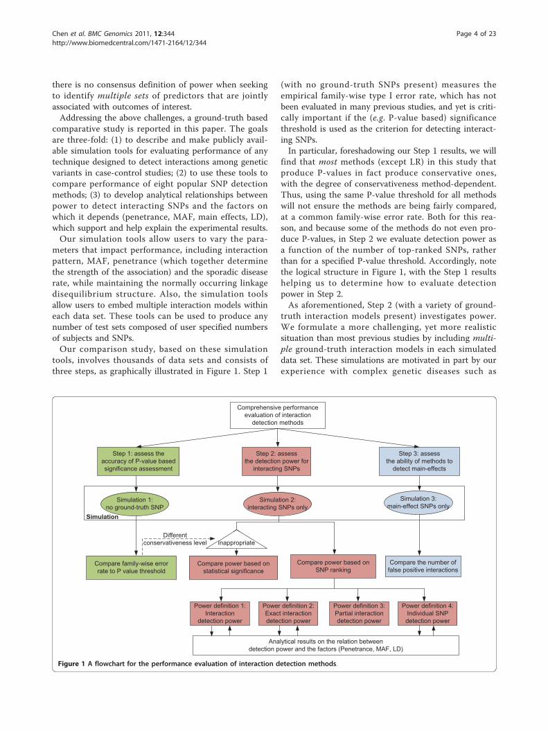
tools, involves thousands of data sets and consists ofthree steps, as graphically illustrated in Figure 1. Step 1

(with no ground-truth SNPs present) measures theempirical family-wise type I error rate, which has notbeen evaluated in many previous studies, and yet is criti-cally important if the (e.g. P-value based) significancethreshold is used as the criterion for detecting interact-ing SNPs.In particular, foreshadowing our Step 1 results, we will

find that most methods (except LR) in this study thatproduce P-values in fact produce conservative ones,with the degree of conservativeness method-dependent.Thus, using the same P-value threshold for all methodswill not ensure the methods are being fairly compared,at a common family-wise error rate. Both for this rea-son, and because some of the methods do not even pro-duce P-values, in Step 2 we evaluate detection power asa function of the number of top-ranked SNPs, ratherthan for a specified P-value threshold. Accordingly, notethe logical structure in Figure 1, with the Step 1 resultshelping us to determine how to evaluate detectionpower in Step 2.As aforementioned, Step 2 (with a variety of ground-

truth interaction models present) investigates power.We formulate a more challenging, yet more realisticsituation than most previous studies by including multi-ple ground-truth interaction models in each simulateddata set. These simulations are motivated in part by ourexperience with complex genetic diseases such as

Comprehensive performanceevaluation of interaction

detection methods

Step 1: assess theaccuracy of P-value basedsignificance assessment

Step 2: assessthe detection power for

interacting SNPs

Compare power based onstatistical significance

Compare power based onSNP ranking

Power definition 1:Interaction

detection power

Power definition 2:Exact interactiondetection power

Power definition 3:Partial interactiondetection power

Power definition 4:Individual SNPdetection power

Step 3: assessthe ability of methods to

detect main-effects

Differentconservativeness level

Compare family-wise errorrate to P value threshold

Compare the number offalse positive interactions

Simulation 1:no ground-truth SNP

Simulation 2:interacting SNPs only

Simulation 3:main-effect SNPs only

Inappropriate

Simulation

Analytical results on the relation betweendetection power and the factors (Penetrance, MAF, LD)

Figure 1 A flowchart for the performance evaluation of interaction detection methods.


of 23

autoimmune diseases, diabetes and end-stage renal dis-ease [18,19,56,57]. In total, ninety different interactionmodels are investigated in this study, jointly determinedby 5 underlying interaction types and 3 parameters, con-trolling penetrance, MAF, and LD. Step 3 investigatesthe power to detect main effect SNPs, i.e. we investigatehow the methods (many of which are designed to detectboth interactions and main effect SNPs) perform whenonly main effects are present in the data.The main contributions and novelty of our compari-

son study are: (1) comprehensive comparison of state-of-the-art techniques on realistic simulated data sets,each of which includes multiple interaction models; (2)new proposed power criteria, well-matched to distinctGWAS applications (e.g., detection of “at least one SNPin an interaction”); (3) evaluation of the accuracy of (P-value based) significance assessments made by thedetection methods; (4) investigation of detection ofmodels with variable order interactions (up to 5thorder) in SNP data sets; (5) new analytical results on therelationship between interaction parameters and statisti-cal power; (6) investigation of the flexibility of interac-tion-detection methods, i.e. whether (and with whataccuracy) they can detect both interactions and maineffects; (7) discoveries concerning relative performanceof methods (e.g., comparative evaluation of the promis-ing recent method, MECPM). Since we are presenting adiversity of results, both experimental and analytical, toassist the reader in navigating our work, Figure 1 gives agraphical summary of our experimental steps, the resultsproduced there from, and the connections between thedifferent results, both experimental and analytical.

ResultsExperimental Design and ProtocolWe selected eight representative methods for evaluation,based on their reported effectiveness and computationalefficiency. Seven of them (MDR, FIM, IG, BEAM, SH,MECPM and LRIT) are designed to detect interactingloci, with the remaining one based on the widely-usedlogistic regression model (LR). LR, using only maineffect terms, serves as a baseline method to compareagainst all the interaction-detection methods, i.e., to seewhether they give any advantage over pure “main effect”methods when the goal is simply to detect the subset ofSNPs that either individually, or via interactions, arepredictive of the phenotype. The description of the eightmethods is given in the “Methods” part.Simulation Data SetsEach data set contains individuals simulated from thecontrol subjects genotyped by the 317K-SNP IlluminaHumanHap300 BeadChip as part of the New York CityCancer Control Project (NYCCCP). To facilitate thisinvestigation [40], a flexible simulation program was

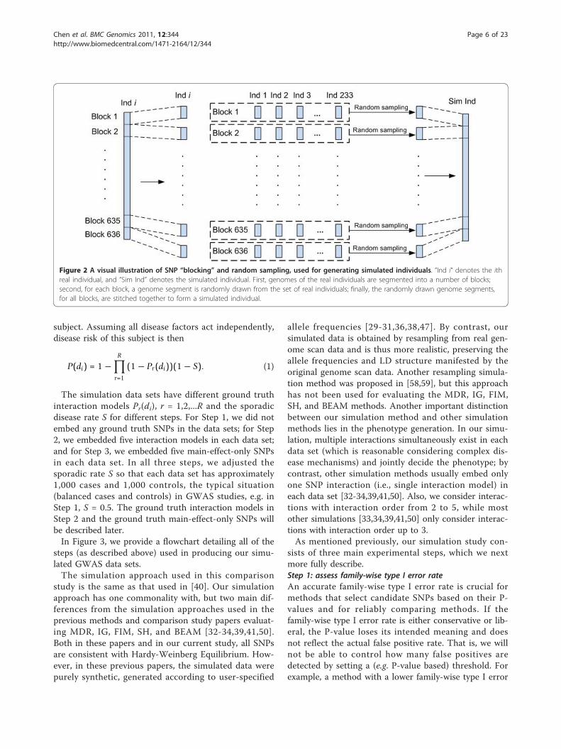
written that generates user defined sample size, numberof SNPs, no missing data or missing data patterns con-sistent with the observed missing data in the originalgenome scan, and affected or unaffected disease statusunder the null hypothesis (i.e., no associations in thegenome) or under the alternative hypothesis (i.e., hard-coded penetrance functions). Missing data is filled incompletely at random and proportional to the allele fre-quencies in the original data. The data sets were pro-duced as follows. Consider a matrix with 223 rowscorresponding to NYCCCP individuals and 317,503 col-umns corresponding to the 317,503 SNPs. The elementsof this matrix are the individual genotypes. The columnswere partitioned into blocks of 500 SNPs, i.e. 636blocks, with the last block containing only 3 SNPs. Thesimulated genome scan data for each individual wasobtained by random draws (with replacement) from areal data matrix of 223 individuals and 636 blocks of500 SNPs. Specifically, the simulated data for an indivi-dual was generated by randomly selecting the first blockfrom the 223 individuals (rows), randomly selecting withreplacement the second block from the 223 individuals,randomly selecting with replacement the third blockfrom the 223 individuals, and so on. Thus the dataretains the basic patterns of linkage disequilibrium (bro-ken by strong recombination hotspots), missing data,and allele frequencies observed in the original genomescan data. The exception to this is only at the 635breaks in the genome corresponding to the blockboundaries. Figure 2 visually illustrates this simulationapproach for randomly resampling genome scan datastarting from the real NYCCP scans. The simulationspresented here correspond to approximately 2000 sub-jects simulated under the alternative hypothesisdescribed below and no missing data. Only autosomalloci are considered in the data.The eight methods were applied to sets of

1000~10,000 SNPs selected at random from the autoso-mal loci. This number of SNPs is consistent with aGWAS study following an initial SNP screening stageand also with pathway-based association studies. Whenselecting SNPs, we first removed those with genotypesthat significantly deviate from Hardy-Weinberg equili-brium, and then selected the desired number of ground-truth and “null” SNPs. For each replication data set,ground-truth SNPs were randomly selected, accordingto the requirements of MAF (within a narrow windowof tolerance), and “null” SNPs were chosen completelyat random. The simulations reported assume that thedisease risk is explained by several ground-truth interac-tion models and the sporadic disease rate S, whichaccounts for the missing heritability and other disease-related factors. Let Pr(di), r = 1,2,...,R be the diseaseprobability generated by R interaction models for the ith


of 23

subject. Assuming all disease factors act independently,disease risk of this subject is then

P(di) = 1 −R∏r=1

(1 − Pr(di))(1 − S). (1)

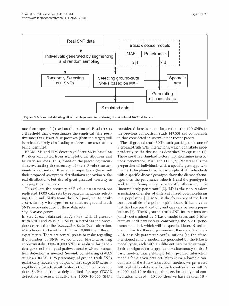
The simulation data sets have different ground truthinteraction models Pr(di), r = 1,2,...R and the sporadicdisease rate S for different steps. For Step 1, we did notembed any ground truth SNPs in the data sets; for Step2, we embedded five interaction models in each data set;and for Step 3, we embedded five main-effect-only SNPsin each data set. In all three steps, we adjusted thesporadic rate S so that each data set has approximately1,000 cases and 1,000 controls, the typical situation(balanced cases and controls) in GWAS studies, e.g. inStep 1, S = 0.5. The ground truth interaction models inStep 2 and the ground truth main-effect-only SNPs willbe described later.In Figure 3, we provide a flowchart detailing all of the

steps (as described above) used in producing our simu-lated GWAS data sets.The simulation approach used in this comparison

study is the same as that used in [40]. Our simulationapproach has one commonality with, but two main dif-ferences from the simulation approaches used in theprevious methods and comparison study papers evaluat-ing MDR, IG, FIM, SH, and BEAM [32-34,39,41,50].Both in these papers and in our current study, all SNPsare consistent with Hardy-Weinberg Equilibrium. How-ever, in these previous papers, the simulated data werepurely synthetic, generated according to user-specified

allele frequencies [29-31,36,38,47]. By contrast, oursimulated data is obtained by resampling from real gen-ome scan data and is thus more realistic, preserving theallele frequencies and LD structure manifested by theoriginal genome scan data. Another resampling simula-tion method was proposed in [58,59], but this approachhas not been used for evaluating the MDR, IG, FIM,SH, and BEAM methods. Another important distinctionbetween our simulation method and other simulationmethods lies in the phenotype generation. In our simu-lation, multiple interactions simultaneously exist in eachdata set (which is reasonable considering complex dis-ease mechanisms) and jointly decide the phenotype; bycontrast, other simulation methods usually embed onlyone SNP interaction (i.e., single interaction model) ineach data set [32-34,39,41,50]. Also, we consider interac-tions with interaction order from 2 to 5, while mostother simulations [33,34,39,41,50] only consider interac-tions with interaction order up to 3.As mentioned previously, our simulation study con-

sists of three main experimental steps, which we nextmore fully describe.Step 1: assess family-wise type I error rateAn accurate family-wise type I error rate is crucial formethods that select candidate SNPs based on their P-values and for reliably comparing methods. If thefamily-wise type I error rate is either conservative or lib-eral, the P-value loses its intended meaning and doesnot reflect the actual false positive rate. That is, we willnot be able to control how many false positives aredetected by setting a (e.g. P-value based) threshold. Forexample, a method with a lower family-wise type I error

Figure 2 A visual illustration of SNP “blocking” and random sampling, used for generating simulated individuals. “Ind i“ denotes the ithreal individual, and “Sim Ind” denotes the simulated individual. First, genomes of the real individuals are segmented into a number of blocks;second, for each block, a genome segment is randomly drawn from the set of real individuals; finally, the randomly drawn genome segments,for all blocks, are stitched together to form a simulated individual.


of 23

rate than expected (based on the estimated P-value) setsa threshold that overestimates the empirical false posi-tive rate; thus, fewer false positives (than the target) willbe selected, likely also leading to fewer true associationsbeing identified.BEAM, SH and FIM detect significant SNPs based on

P-values calculated from asymptotic distributions andheuristic searches. Thus, based on the preceding discus-sion, evaluating the accuracy of their P-value assess-ments is not only of theoretical importance (how welltheir proposed asymptotic distributions approximate thereal distribution), but also of great practical necessity inapplying these methods.To evaluate the accuracy of P-value assessment, we

replicated 1,000 data sets by repeatedly randomly select-ing 1,000 null SNPs from the SNP pool, i.e. to easilyassess family-wise type I error rate, no ground-truthSNPs were embedded in these data sets.Step 2: assess powerIn step 2, each data set has N SNPs, with 15 ground-truth SNPs and N-15 null SNPs, selected via the proce-dure described in the “Simulation Data Sets“ subsection.N is chosen to be either 1000 or 10,000 for differentexperiments. There are several points to make regardingthe number of SNPs we consider. First, assumingapproximately 1000~10,000 SNPs is realistic for candi-date gene and biological pathway studies where interac-tion detection is needed. Second, considering GWASstudies, a 0.15%~1.5% percentage of ground-truth SNPsrealistically models the output of first stage SNP screen-ing/filtering (which greatly reduces the number of candi-date SNPs) in the widely-applied 2-stage GWASdetection process. Finally, the 1000~10,000 SNPs

considered here is much larger than the 100 SNPs inthe previous comparison study [49,50] and comparableto that considered in several other recent papers.The 15 ground-truth SNPs each participate in one of

5 ground-truth SNP interactions, which contribute inde-pendently to the disease, as described by equation (1).There are three standard factors that determine interac-tions: penetrance, MAF and LD [3,7]. Penetrance is theproportion of individuals with a specific genotype whomanifest the phenotype. For example, if all individualswith a specific disease genotype show the disease pheno-type, then the penetrance value is 1 and the genotype issaid to be “completely penetrant"; otherwise, it is“incompletely penetrant” [3]. LD is the non-randomassociation of alleles of different linked polymorphismsin a population [7]. MAF is the frequency of the leastcommon allele of a polymorphic locus. It has a valuethat lies between 0 and 0.5, and can vary between popu-lations [7]. The 5 ground-truth SNP interactions arejointly determined by 5 basic model types and 3 (dis-crete-valued) parameters, controlling the MAF, pene-trance, and LD, which will be specified later. Based onthe choices for these 3 parameters, there are 3 × 3 × 2= 18 possible parameter configurations (so the afore-mentioned ninety models are generated by the 5 basicmodel types, each with 18 different parameter settings).Each configuration is applied simultaneously to the 5basic models, thus yielding 5 fully specified interactionmodels for a given data set. With some allowable ran-domness in the 5 new interaction models, we generated100 replication data sets for each configuration with N= 1000, and 10 replication data sets for one typical con-figuration with N = 10,000; thus we have in total 18 ×

Real SNP data

Individuals generated by segmentingand random sampling

Generatingdisease status

Selecting ground-truthSNPs based on MAF

MAF Penetrance

Basic disease models

Randomly Selectingnull SNPs

Simulated data

x x

Sporadicrate

Figure 3 A flowchart detailing all of the steps used in producing the simulated GWAS data sets.


of 23

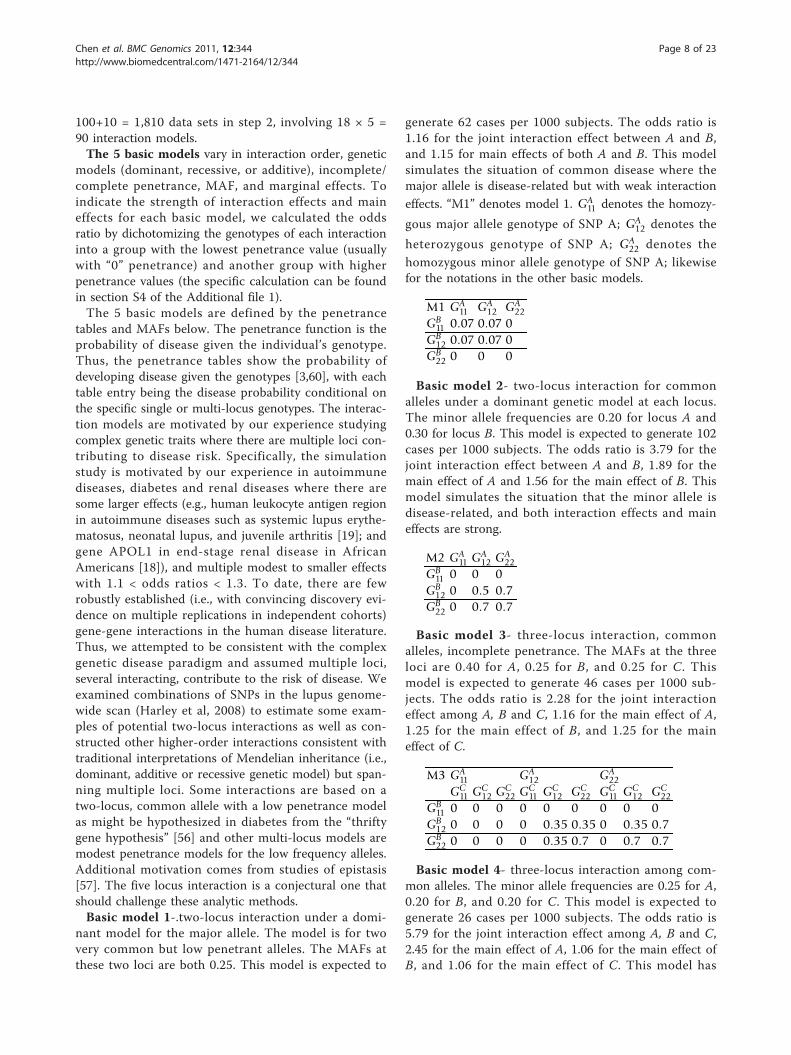
100+10 = 1,810 data sets in step 2, involving 18 × 5 =90 interaction models.The 5 basic models vary in interaction order, genetic

models (dominant, recessive, or additive), incomplete/complete penetrance, MAF, and marginal effects. Toindicate the strength of interaction effects and maineffects for each basic model, we calculated the oddsratio by dichotomizing the genotypes of each interactioninto a group with the lowest penetrance value (usuallywith “0” penetrance) and another group with higherpenetrance values (the specific calculation can be foundin section S4 of the Additional file 1).The 5 basic models are defined by the penetrance

tables and MAFs below. The penetrance function is theprobability of disease given the individual’s genotype.Thus, the penetrance tables show the probability ofdeveloping disease given the genotypes [3,60], with eachtable entry being the disease probability conditional onthe specific single or multi-locus genotypes. The interac-tion models are motivated by our experience studyingcomplex genetic traits where there are multiple loci con-tributing to disease risk. Specifically, the simulationstudy is motivated by our experience in autoimmunediseases, diabetes and renal diseases where there aresome larger effects (e.g., human leukocyte antigen regionin autoimmune diseases such as systemic lupus erythe-matosus, neonatal lupus, and juvenile arthritis [19]; andgene APOL1 in end-stage renal disease in AfricanAmericans [18]), and multiple modest to smaller effectswith 1.1 < odds ratios < 1.3. To date, there are fewrobustly established (i.e., with convincing discovery evi-dence on multiple replications in independent cohorts)gene-gene interactions in the human disease literature.Thus, we attempted to be consistent with the complexgenetic disease paradigm and assumed multiple loci,several interacting, contribute to the risk of disease. Weexamined combinations of SNPs in the lupus genome-wide scan (Harley et al, 2008) to estimate some exam-ples of potential two-locus interactions as well as con-structed other higher-order interactions consistent withtraditional interpretations of Mendelian inheritance (i.e.,dominant, additive or recessive genetic model) but span-ning multiple loci. Some interactions are based on atwo-locus, common allele with a low penetrance modelas might be hypothesized in diabetes from the “thriftygene hypothesis” [56] and other multi-locus models aremodest penetrance models for the low frequency alleles.Additional motivation comes from studies of epistasis[57]. The five locus interaction is a conjectural one thatshould challenge these analytic methods.Basic model 1-.two-locus interaction under a domi-

nant model for the major allele. The model is for twovery common but low penetrant alleles. The MAFs atthese two loci are both 0.25. This model is expected to

generate 62 cases per 1000 subjects. The odds ratio is1.16 for the joint interaction effect between A and B,and 1.15 for main effects of both A and B. This modelsimulates the situation of common disease where themajor allele is disease-related but with weak interactioneffects. “M1” denotes model 1. GA

11 denotes the homozy-

gous major allele genotype of SNP A; GA12 denotes the

heterozygous genotype of SNP A; GA22 denotes the

homozygous minor allele genotype of SNP A; likewisefor the notations in the other basic models.

M1 GA11 GA

12 GA22

GB11 0.07 0.07 0

GB12 0.07 0.07 0

GB22 0 0 0

Basic model 2- two-locus interaction for commonalleles under a dominant genetic model at each locus.The minor allele frequencies are 0.20 for locus A and0.30 for locus B. This model is expected to generate 102cases per 1000 subjects. The odds ratio is 3.79 for thejoint interaction effect between A and B, 1.89 for themain effect of A and 1.56 for the main effect of B. Thismodel simulates the situation that the minor allele isdisease-related, and both interaction effects and maineffects are strong.

M2 GA11 GA

12 GA22

GB11 0 0 0

GB12 0 0.5 0.7

GB22 0 0.7 0.7

Basic model 3- three-locus interaction, commonalleles, incomplete penetrance. The MAFs at the threeloci are 0.40 for A, 0.25 for B, and 0.25 for C. Thismodel is expected to generate 46 cases per 1000 sub-jects. The odds ratio is 2.28 for the joint interactioneffect among A, B and C, 1.16 for the main effect of A,1.25 for the main effect of B, and 1.25 for the maineffect of C.

M3 GA11 GA

12 GA22

GC11 GC

12 GC22 GC

11 GC12 GC

22 GC11 GC

12 GC22

GB11 0 0 0 0 0 0 0 0 0

GB12 0 0 0 0 0.35 0.35 0 0.35 0.7

GB22 0 0 0 0 0.35 0.7 0 0.7 0.7

Basic model 4- three-locus interaction among com-mon alleles. The minor allele frequencies are 0.25 for A,0.20 for B, and 0.20 for C. This model is expected togenerate 26 cases per 1000 subjects. The odds ratio is5.79 for the joint interaction effect among A, B and C,2.45 for the main effect of A, 1.06 for the main effect ofB, and 1.06 for the main effect of C. This model has


of 23

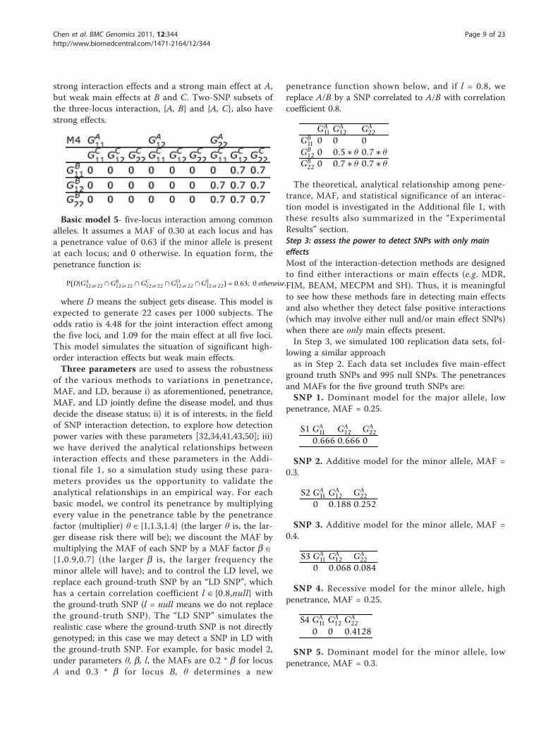
strong interaction effects and a strong main effect at A,but weak main effects at B and C. Two-SNP subsets ofthe three-locus interaction, {A, B} and {A, C}, also havestrong effects.

Basic model 5- five-locus interaction among commonalleles. It assumes a MAF of 0.30 at each locus and hasa penetrance value of 0.63 if the minor allele is presentat each locus; and 0 otherwise. In equation form, thepenetrance function is:

P(D|GA12 or 22 ∩ GB

12 or 22 ∩ GC12 or 22 ∩ GD

12 or 22 ∩ GE12 or 22) = 0.63; 0 otherwise,

where D means the subject gets disease. This model isexpected to generate 22 cases per 1000 subjects. Theodds ratio is 4.48 for the joint interaction effect amongthe five loci, and 1.09 for the main effect at all five loci.This model simulates the situation of significant high-order interaction effects but weak main effects.Three parameters are used to assess the robustness

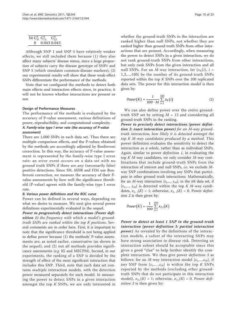
of the various methods to variations in penetrance,MAF, and LD, because i) as aforementioned, penetrance,MAF, and LD jointly define the disease model, and thusdecide the disease status; ii) it is of interests, in the fieldof SNP interaction detection, to explore how detectionpower varies with these parameters [32,34,41,43,50]; iii)we have derived the analytical relationships betweeninteraction effects and these parameters in the Addi-tional file 1, so a simulation study using these para-meters provides us the opportunity to validate theanalytical relationships in an empirical way. For eachbasic model, we control its penetrance by multiplyingevery value in the penetrance table by the penetrancefactor (multiplier) θ Î{1,1.3,1.4} (the larger θ is, the lar-ger disease risk there will be); we discount the MAF bymultiplying the MAF of each SNP by a MAF factor b Î{1,0.9,0.7} (the larger b is, the larger frequency theminor allele will have); and to control the LD level, wereplace each ground-truth SNP by an “LD SNP”, whichhas a certain correlation coefficient l Î{0.8,null} withthe ground-truth SNP (l = null means we do not replacethe ground-truth SNP). The “LD SNP” simulates therealistic case where the ground-truth SNP is not directlygenotyped; in this case we may detect a SNP in LD withthe ground-truth SNP. For example, for basic model 2,under parameters θ, b, l, the MAFs are 0.2 * b for locusA and 0.3 * b for locus B, θ determines a new

penetrance function shown below, and if l = 0.8, wereplace A/B by a SNP correlated to A/B with correlationcoefficient 0.8.

GA11 GA

12 GA22

GB11 0 0 0

GB12 0 0.5 ∗ θ 0.7 ∗ θ

GB22 0 0.7 ∗ θ 0.7 ∗ θ

The theoretical, analytical relationship among pene-trance, MAF, and statistical significance of an interac-tion model is investigated in the Additional file 1, withthese results also summarized in the “ExperimentalResults” section.Step 3: assess the power to detect SNPs with only maineffectsMost of the interaction-detection methods are designedto find either interactions or main effects (e.g. MDR,FIM, BEAM, MECPM and SH). Thus, it is meaningfulto see how these methods fare in detecting main effectsand also whether they detect false positive interactions(which may involve either null and/or main effect SNPs)when there are only main effects present.In Step 3, we simulated 100 replication data sets, fol-

lowing a similar approachas in Step 2. Each data set includes five main-effect

ground truth SNPs and 995 null SNPs. The penetrancesand MAFs for the five ground truth SNPs are:SNP 1. Dominant model for the major allele, low

penetrance, MAF = 0.25.

S1 GA11 GA

12 GA22

0.666 0.666 0

SNP 2. Additive model for the minor allele, MAF =0.3.

S2 GA11 GA

12 GA22

0 0.188 0.252

SNP 3. Additive model for the minor allele, MAF =0.4.

S3 GA11 GA

12 GA22

0 0.068 0.084

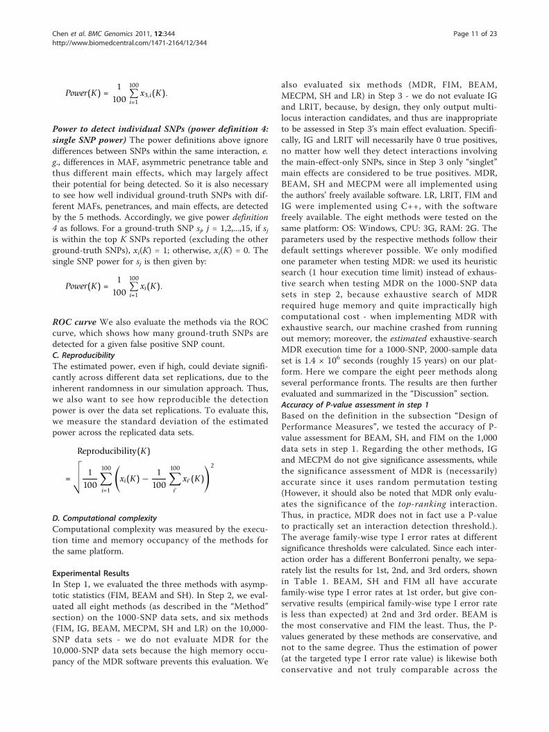
SNP 4. Recessive model for the minor allele, highpenetrance, MAF = 0.25.

S4 GA11 GA

12 GA22

0 0 0.4128

SNP 5. Dominant model for the minor allele, lowpenetrance, MAF = 0.3.


of 23

S4 GA11 GA

12 GA22

0 0.043 0.043

Although SNP 1 and SNP 5 have relatively weakereffects, we still included them because (1) they alsoaffect many subjects’ disease status, since a large propor-tion of subjects carry the disease genotype of SNP1 andSNP 5 (which simulates common-disease markers); (2)our experimental results will show that these weak-effectSNPs differentiate the performance of the methods.Note that we configured the methods to detect both

main effects and interaction effects since, in practice, itwill not be known whether interactions are present ornot.

Design of Performance MeasuresThe performance of the methods is evaluated by theaccuracy of P-value assessment, various definitions ofpower, reproducibility, and computational complexity.A. Family-wise type I error rate (the accuracy of P-valueassessment)There are 1,000 SNPs in each data set. Thus there aremultiple comparison effects, and the P-values obtainedby the methods are accordingly adjusted by Bonferronicorrection. In this way, the accuracy of P-value assess-ment is represented by the family-wise type I errorrate: an error event occurs on a data set with noground truth SNPs if there are any (necessarily false)positive detections. Since SH, MDR and FIM use Bon-ferroni correction, we measure the accuracy of their P-value assessments by how well the significance thresh-old (P-value) agrees with the family-wise type I errorrate.B. Various power definitions and the ROC curvePower can be defined in several ways, depending onwhat we desire to measure. We next give several powerdefinitions experimentally evaluated in the sequel.Power to progressively detect interactions (Power defi-nition 1) the frequency with which a model’s ground-truth SNPs are ranked within the top K positions. Sev-eral comments are in order here. First, it is important tonote that the significance threshold is not being appliedto define power because (1) the methods’ P-value assess-ments are, as noted earlier, conservative (as shown inthe sequel), and (2) not all methods provides signifi-cance assessments (e.g. IG and MECPM). Second, in ourexperiments, the ranking of a SNP is decided by thestrength of effect of the most significant interaction thatincludes this SNP. Third, note that each data set con-tains multiple interaction models, with the detectionpower measured separately for each model. In measur-ing the power to detect SNPs in a given interactionamongst the top K SNPs, we are only interested in

whether the ground-truth SNPs in the interaction areranked higher than null SNPs, not whether they areranked higher than ground-truth SNPs from other inter-actions that are present. Accordingly, when measuringthe power to detect SNPs in a given interaction, we donot rank ground-truth SNPs from other interactions,but only rank SNPs from the given interaction and allnull SNPs. For an M-way interaction, let {xK(i), i =1,2,...,100} be the number of its ground-truth SNPsreported within the top K SNPs over the 100 replicateddata sets. The power for this interaction model is thengiven by:

Power(K) =1

100 · M100∑i=1

xK(i) (2)

We can also define power over the entire ground-truth SNP set by setting M = 15 and considering allground-truth SNPs in the ranking.Power to precisely detect interactions (power defini-tion 2: exact interaction power) for an M-way ground-truth interaction, how likely it is detected amongst thetop K M-way candidates produced by a method. Thispower definition evaluates the sensitivity to detect theinteraction as a whole, rather than as individual SNPs.Again, similar to power definition 1, in evaluating thetop K M-way candidates, we only consider M-way com-binations that include ground-truth SNPs from theinteraction of interest and null SNPs, i.e. we exclude M-way SNP combinations involving any SNPs that partici-pate in other ground truth interactions. Mathematically,for an M-way interaction {s1,..., sM}, in the ith data set, if{s1,..., sM} is detected within the top K M-way candi-dates, x2, i(K) = 1; otherwise, x2, i(K) = 0. Power defini-tion 2 is then given by:

Power(K) =1

100

100∑i=1

x2,i(K)

Power to detect at least 1 SNP in the ground-truthinteraction (power definition 3: partial interactionpower) As revealed by the definitions of the interac-tion models, a subset of the interacting SNPs mayhave strong association to disease risk. Detecting aninteraction subset should be acceptable since thisgives a good “clue” to help further identify the com-plete interaction. We thus give power definition 3 asfollows: for an M-way interaction model {s1,...,sM}, ifany SNP from {s1,. . . ,sM} is within the top K SNPsreported by the methods (excluding other ground-truth SNPs that do not participate in this interactionmodel), x3,i(K) = 1; otherwise, x3,i(K) = 0. Power defi-nition 3 is then given by:


of 23

Power(K) =1

100

100∑i=1

x3,i(K).

Power to detect individual SNPs (power definition 4:single SNP power) The power definitions above ignoredifferences between SNPs within the same interaction, e.g., differences in MAF, asymmetric penetrance table andthus different main effects, which may largely affecttheir potential for being detected. So it is also necessaryto see how well individual ground-truth SNPs with dif-ferent MAFs, penetrances, and main effects, are detectedby the 5 methods. Accordingly, we give power definition4 as follows. For a ground-truth SNP sj, j = 1,2,...,15, if sjis within the top K SNPs reported (excluding the otherground-truth SNPs), xi(K) = 1; otherwise, xi(K) = 0. Thesingle SNP power for sj is then given by:

Power(K) =1

100

100∑i=1

xi(K).

ROC curve We also evaluate the methods via the ROCcurve, which shows how many ground-truth SNPs aredetected for a given false positive SNP count.C. ReproducibilityThe estimated power, even if high, could deviate signifi-cantly across different data set replications, due to theinherent randomness in our simulation approach. Thus,we also want to see how reproducible the detectionpower is over the data set replications. To evaluate this,we measure the standard deviation of the estimatedpower across the replicated data sets.

Reproducibility(K)

=

√√√√ 1100

100∑i=1

(xi(K) − 1

100

100∑i′

xi′(K)

)2

D. Computational complexityComputational complexity was measured by the execu-tion time and memory occupancy of the methods forthe same platform.

Experimental ResultsIn Step 1, we evaluated the three methods with asymp-totic statistics (FIM, BEAM and SH). In Step 2, we eval-uated all eight methods (as described in the “Method”section) on the 1000-SNP data sets, and six methods(FIM, IG, BEAM, MECPM, SH and LR) on the 10,000-SNP data sets - we do not evaluate MDR for the10,000-SNP data sets because the high memory occu-pancy of the MDR software prevents this evaluation. We

also evaluated six methods (MDR, FIM, BEAM,MECPM, SH and LR) in Step 3 - we do not evaluate IGand LRIT, because, by design, they only output multi-locus interaction candidates, and thus are inappropriateto be assessed in Step 3’s main effect evaluation. Specifi-cally, IG and LRIT will necessarily have 0 true positives,no matter how well they detect interactions involvingthe main-effect-only SNPs, since in Step 3 only “singlet”main effects are considered to be true positives. MDR,BEAM, SH and MECPM were all implemented usingthe authors’ freely available software. LR, LRIT, FIM andIG were implemented using C++, with the softwarefreely available. The eight methods were tested on thesame platform: OS: Windows, CPU: 3G, RAM: 2G. Theparameters used by the respective methods follow theirdefault settings wherever possible. We only modifiedone parameter when testing MDR: we used its heuristicsearch (1 hour execution time limit) instead of exhaus-tive search when testing MDR on the 1000-SNP datasets in step 2, because exhaustive search of MDRrequired huge memory and quite impractically highcomputational cost - when implementing MDR withexhaustive search, our machine crashed from runningout memory; moreover, the estimated exhaustive-searchMDR execution time for a 1000-SNP, 2000-sample dataset is 1.4 × 106 seconds (roughly 15 years) on our plat-form. Here we compare the eight peer methods alongseveral performance fronts. The results are then furtherevaluated and summarized in the “Discussion” section.Accuracy of P-value assessment in step 1Based on the definition in the subsection “Design ofPerformance Measures”, we tested the accuracy of P-value assessment for BEAM, SH, and FIM on the 1,000data sets in step 1. Regarding the other methods, IGand MECPM do not give significance assessments, whilethe significance assessment of MDR is (necessarily)accurate since it uses random permutation testing(However, it should also be noted that MDR only evalu-ates the significance of the top-ranking interaction.Thus, in practice, MDR does not in fact use a P-valueto practically set an interaction detection threshold.).The average family-wise type I error rates at differentsignificance thresholds were calculated. Since each inter-action order has a different Bonferroni penalty, we sepa-rately list the results for 1st, 2nd, and 3rd orders, shownin Table 1. BEAM, SH and FIM all have accuratefamily-wise type I error rates at 1st order, but give con-servative results (empirical family-wise type I error rateis less than expected) at 2nd and 3rd order. BEAM isthe most conservative and FIM the least. Thus, the P-values generated by these methods are conservative, andnot to the same degree. Thus the estimation of power(at the targeted type I error rate value) is likewise bothconservative and not truly comparable across the


of 23

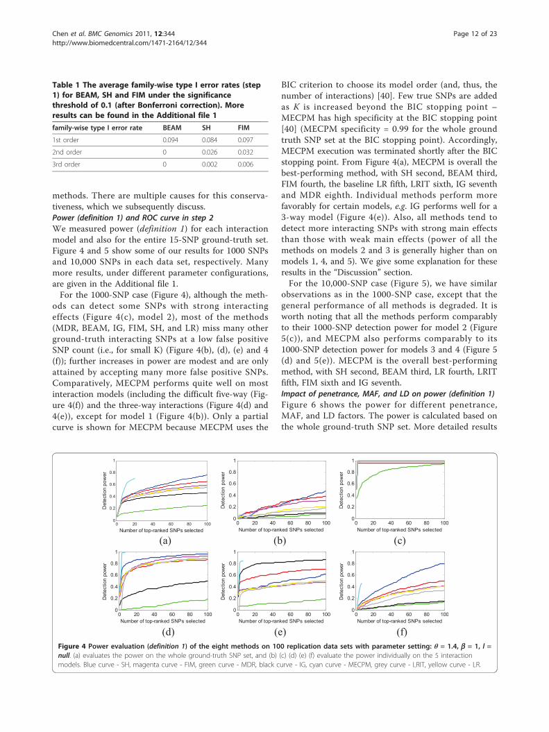
methods. There are multiple causes for this conserva-tiveness, which we subsequently discuss.Power (definition 1) and ROC curve in step 2We measured power (definition 1) for each interactionmodel and also for the entire 15-SNP ground-truth set.Figure 4 and 5 show some of our results for 1000 SNPsand 10,000 SNPs in each data set, respectively. Manymore results, under different parameter configurations,are given in the Additional file 1.For the 1000-SNP case (Figure 4), although the meth-

ods can detect some SNPs with strong interactingeffects (Figure 4(c), model 2), most of the methods(MDR, BEAM, IG, FIM, SH, and LR) miss many otherground-truth interacting SNPs at a low false positiveSNP count (i.e., for small K) (Figure 4(b), (d), (e) and 4(f)); further increases in power are modest and are onlyattained by accepting many more false positive SNPs.Comparatively, MECPM performs quite well on mostinteraction models (including the difficult five-way (Fig-ure 4(f)) and the three-way interactions (Figure 4(d) and4(e)), except for model 1 (Figure 4(b)). Only a partialcurve is shown for MECPM because MECPM uses the

BIC criterion to choose its model order (and, thus, thenumber of interactions) [40]. Few true SNPs are addedas K is increased beyond the BIC stopping point –MECPM has high specificity at the BIC stopping point[40] (MECPM specificity = 0.99 for the whole groundtruth SNP set at the BIC stopping point). Accordingly,MECPM execution was terminated shortly after the BICstopping point. From Figure 4(a), MECPM is overall thebest-performing method, with SH second, BEAM third,FIM fourth, the baseline LR fifth, LRIT sixth, IG seventhand MDR eighth. Individual methods perform morefavorably for certain models, e.g. IG performs well for a3-way model (Figure 4(e)). Also, all methods tend todetect more interacting SNPs with strong main effectsthan those with weak main effects (power of all themethods on models 2 and 3 is generally higher than onmodels 1, 4, and 5). We give some explanation for theseresults in the “Discussion” section.For the 10,000-SNP case (Figure 5), we have similar

observations as in the 1000-SNP case, except that thegeneral performance of all methods is degraded. It isworth noting that all the methods perform comparablyto their 1000-SNP detection power for model 2 (Figure5(c)), and MECPM also performs comparably to its1000-SNP detection power for models 3 and 4 (Figure 5(d) and 5(e)). MECPM is the overall best-performingmethod, with SH second, BEAM third, LR fourth, LRITfifth, FIM sixth and IG seventh.Impact of penetrance, MAF, and LD on power (definition 1)Figure 6 shows the power for different penetrance,MAF, and LD factors. The power is calculated based onthe whole ground-truth SNP set. More detailed results

Table 1 The average family-wise type I error rates (step1) for BEAM, SH and FIM under the significancethreshold of 0.1 (after Bonferroni correction). Moreresults can be found in the Additional file 1

family-wise type I error rate BEAM SH FIM

1st order 0.094 0.084 0.097

2nd order 0 0.026 0.032

3rd order 0 0.002 0.006

0 20 40 60 80 1000

0.2

0.4

0.6

0.8

1

Det

ectio

n po

wer

Number of top-ranked SNPs selected0 20 40 60 80 100

0

0.2

0.4

0.6

0.8

1

Det

ectio

n po

wer


0

0.2

0.4

0.6

0.8

1

Det

ectio

n po

wer

Number of top-ranked SNPs selected

(a) (b) (c)

0 20 40 60 80 1000

0.2

0.4

0.6

0.8

1

Det

ectio

n po

wer


0

0.2

0.4

0.6

0.8

1

Det

ectio

n po

wer


0

0.2

0.4

0.6

0.8

1

Det

ectio

n po

wer

Number of top-ranked SNPs selected

(d) (e) (f) Figure 4 Power evaluation (definition 1) of the eight methods on 100 replication data sets with parameter setting: θ = 1.4, b = 1, l =null. (a) evaluates the power on the whole ground-truth SNP set, and (b) (c) (d) (e) (f) evaluate the power individually on the 5 interactionmodels. Blue curve - SH, magenta curve - FIM, green curve - MDR, black curve - IG, cyan curve - MECPM, grey curve - LRIT, yellow curve - LR.


of 23

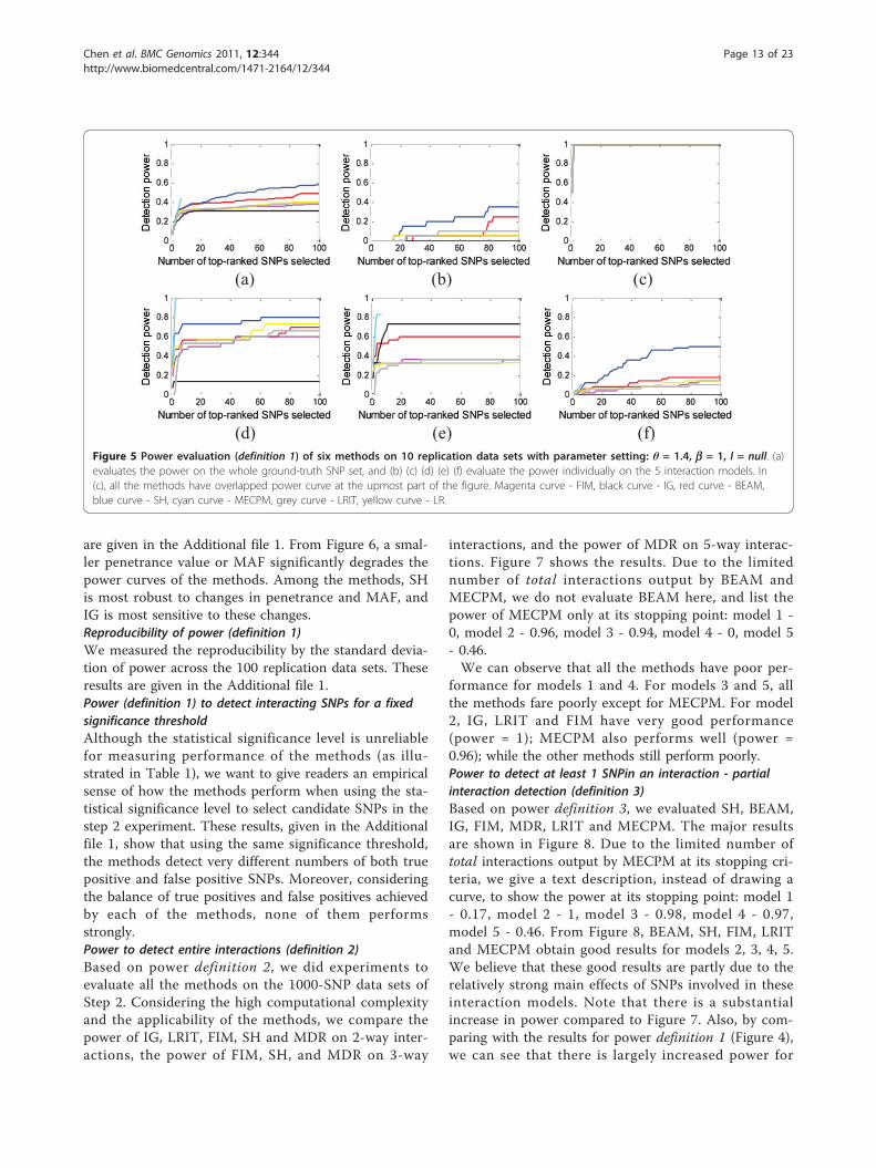
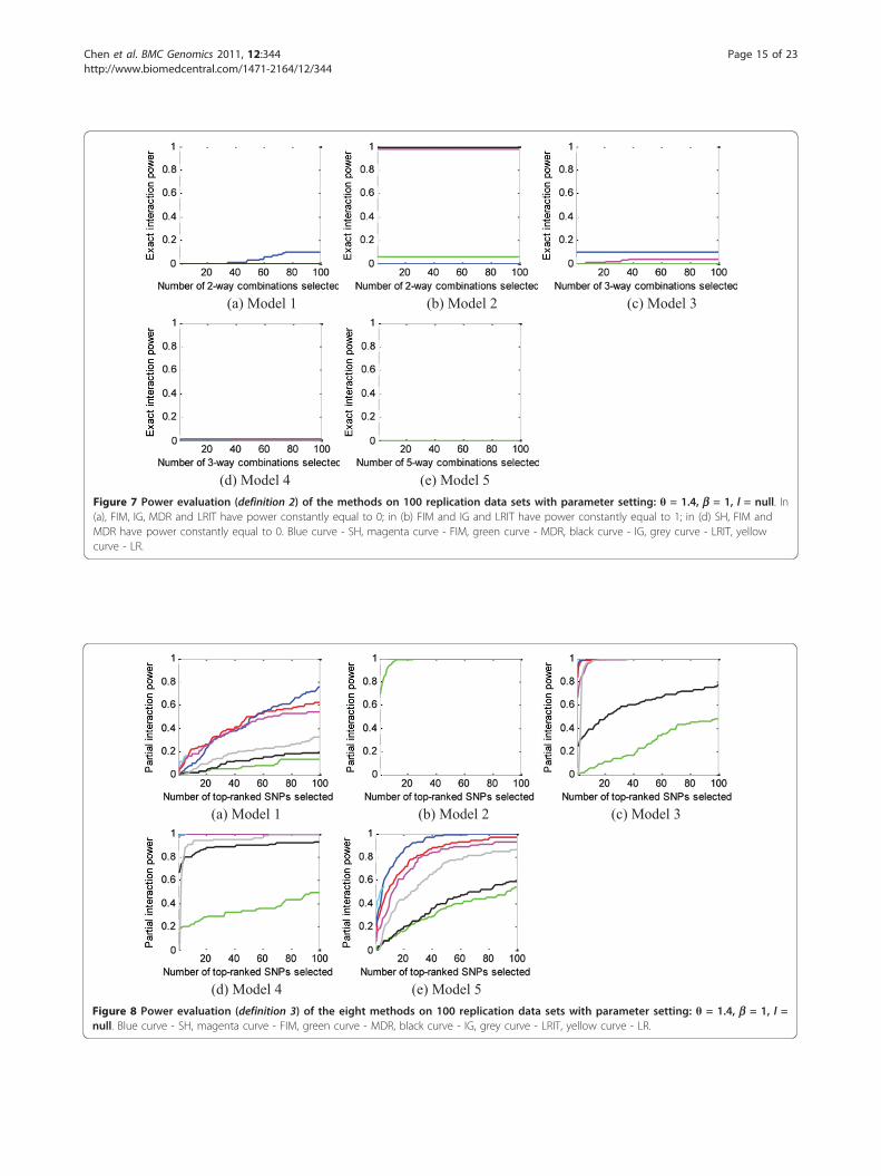
are given in the Additional file 1. From Figure 6, a smal-ler penetrance value or MAF significantly degrades thepower curves of the methods. Among the methods, SHis most robust to changes in penetrance and MAF, andIG is most sensitive to these changes.Reproducibility of power (definition 1)We measured the reproducibility by the standard devia-tion of power across the 100 replication data sets. Theseresults are given in the Additional file 1.Power (definition 1) to detect interacting SNPs for a fixedsignificance thresholdAlthough the statistical significance level is unreliablefor measuring performance of the methods (as illu-strated in Table 1), we want to give readers an empiricalsense of how the methods perform when using the sta-tistical significance level to select candidate SNPs in thestep 2 experiment. These results, given in the Additionalfile 1, show that using the same significance threshold,the methods detect very different numbers of both truepositive and false positive SNPs. Moreover, consideringthe balance of true positives and false positives achievedby each of the methods, none of them performsstrongly.Power to detect entire interactions (definition 2)Based on power definition 2, we did experiments toevaluate all the methods on the 1000-SNP data sets ofStep 2. Considering the high computational complexityand the applicability of the methods, we compare thepower of IG, LRIT, FIM, SH and MDR on 2-way inter-actions, the power of FIM, SH, and MDR on 3-way

interactions, and the power of MDR on 5-way interac-tions. Figure 7 shows the results. Due to the limitednumber of total interactions output by BEAM andMECPM, we do not evaluate BEAM here, and list thepower of MECPM only at its stopping point: model 1 -0, model 2 - 0.96, model 3 - 0.94, model 4 - 0, model 5- 0.46.We can observe that all the methods have poor per-

formance for models 1 and 4. For models 3 and 5, allthe methods fare poorly except for MECPM. For model2, IG, LRIT and FIM have very good performance(power = 1); MECPM also performs well (power =0.96); while the other methods still perform poorly.Power to detect at least 1 SNPin an interaction - partialinteraction detection (definition 3)Based on power definition 3, we evaluated SH, BEAM,IG, FIM, MDR, LRIT and MECPM. The major resultsare shown in Figure 8. Due to the limited number oftotal interactions output by MECPM at its stopping cri-teria, we give a text description, instead of drawing acurve, to show the power at its stopping point: model 1- 0.17, model 2 - 1, model 3 - 0.98, model 4 - 0.97,model 5 - 0.46. From Figure 8, BEAM, SH, FIM, LRITand MECPM obtain good results for models 2, 3, 4, 5.We believe that these good results are partly due to therelatively strong main effects of SNPs involved in theseinteraction models. Note that there is a substantialincrease in power compared to Figure 7. Also, by com-paring with the results for power definition 1 (Figure 4),we can see that there is largely increased power for

(a) (b) (c)

(d) (e) (f) Figure 5 Power evaluation (definition 1) of six methods on 10 replication data sets with parameter setting: θ = 1.4, b = 1, l = null. (a)evaluates the power on the whole ground-truth SNP set, and (b) (c) (d) (e) (f) evaluate the power individually on the 5 interaction models. In(c), all the methods have overlapped power curve at the upmost part of the figure. Magenta curve - FIM, black curve - IG, red curve - BEAM,blue curve - SH, cyan curve - MECPM, grey curve - LRIT, yellow curve - LR.


of 23

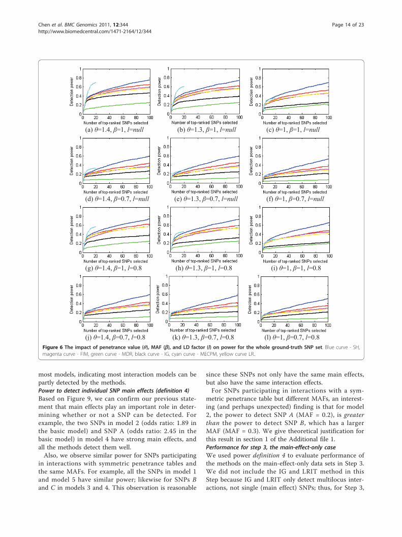
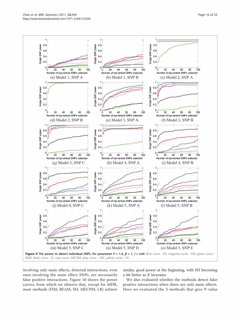
most models, indicating most interaction models can bepartly detected by the methods.Power to detect individual SNP main effects (definition 4)Based on Figure 9, we can confirm our previous state-ment that main effects play an important role in deter-mining whether or not a SNP can be detected. Forexample, the two SNPs in model 2 (odds ratio: 1.89 inthe basic model) and SNP A (odds ratio: 2.45 in thebasic model) in model 4 have strong main effects, andall the methods detect them well.Also, we observe similar power for SNPs participating

in interactions with symmetric penetrance tables andthe same MAFs. For example, all the SNPs in model 1and model 5 have similar power; likewise for SNPs Band C in models 3 and 4. This observation is reasonable

since these SNPs not only have the same main effects,but also have the same interaction effects.For SNPs participating in interactions with a sym-

metric penetrance table but different MAFs, an interest-ing (and perhaps unexpected) finding is that for model2, the power to detect SNP A (MAF = 0.2), is greaterthan the power to detect SNP B, which has a largerMAF (MAF = 0.3). We give theoretical justification forthis result in section 1 of the Additional file 1.Performance for step 3, the main-effect-only caseWe used power definition 4 to evaluate performance ofthe methods on the main-effect-only data sets in Step 3.We did not include the IG and LRIT method in thisStep because IG and LRIT only detect multilocus inter-actions, not single (main effect) SNPs; thus, for Step 3,

(a) =1.4, =1, l=null (b) =1.3, =1, l=null (c) =1, =1, l=null

(d) =1.4, =0.7, l=null (e) =1.3, =0.7, l=null (f) =1, =0.7, l=null

(g) =1.4, =1, l=0.8 (h) =1.3, =1, l=0.8 (i) =1, =1, l=0.8

(j) =1.4, =0.7, l=0.8 (k) =1.3, =0.7, l=0.8 (l) =1, =0.7, l=0.8 Figure 6 The impact of penetrance value (θ), MAF (b), and LD factor (l) on power for the whole ground-truth SNP set. Blue curve - SH,magenta curve - FIM, green curve - MDR, black curve - IG, cyan curve - MECPM, yellow curve LR..


of 23

(a) Model 1 (b) Model 2 (c) Model 3

(d) Model 4 (e) Model 5Figure 7 Power evaluation (definition 2) of the methods on 100 replication data sets with parameter setting: θ = 1.4, b = 1, l = null. In(a), FIM, IG, MDR and LRIT have power constantly equal to 0; in (b) FIM and IG and LRIT have power constantly equal to 1; in (d) SH, FIM andMDR have power constantly equal to 0. Blue curve - SH, magenta curve - FIM, green curve - MDR, black curve - IG, grey curve - LRIT, yellowcurve - LR.

(a) Model 1 (b) Model 2 (c) Model 3

(d) Model 4 (e) Model 5Figure 8 Power evaluation (definition 3) of the eight methods on 100 replication data sets with parameter setting: θ = 1.4, b = 1, l =null. Blue curve - SH, magenta curve - FIM, green curve - MDR, black curve - IG, grey curve - LRIT, yellow curve - LR.


of 23

involving only main effects, detected interactions, evenones involving the main effect SNPs, are necessarilyfalse positive interactions. Figure 10 shows the powercurves, from which we observe that, except for MDR,most methods (FIM, BEAM, SH, MECPM, LR) achieve

similar, good power at the beginning, with SH becominga bit better as K increases.We also evaluated whether the methods detect false

positive interactions when there are only main effects.Here we evaluated the 3 methods that give P-value

(a) Model 1, SNP A (b) Model 1, SNP B (c) Model 2, SNP A

(d) Model 2, SNP B (e) Model 3, SNP A (f) Model 3, SNP B

(g) Model 3, SNP C (h) Model 4, SNP A (i) Model 4, SNP B

(j) Model 4, SNP C (k) Model 5, SNP A (l) Model 5, SNP B

(m) Model 5, SNP C (n) Model 5, SNP D (o) Model 5, SNP E Figure 9 The power to detect individual SNPs, for parameter θ = 1.4, b = 1, l = null. Blue curve - SH, magenta curve - FIM, green curve -MDR, black curve - IG, cyan curve -MECPM, grey curve - LRIT, yellow curve - LR.


of 23

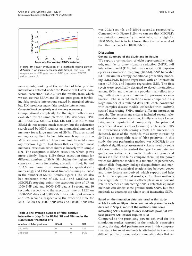
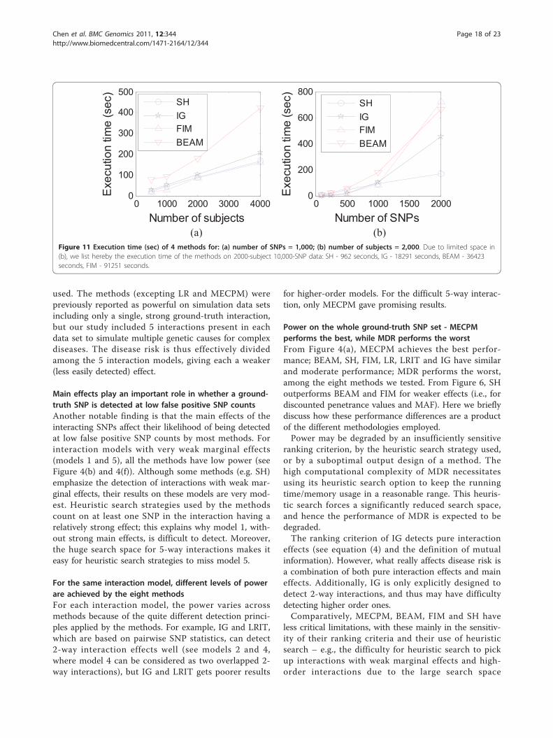
assessments, looking at the number of false positiveinteractions detected under the P-value of 0.1 after Bon-ferroni correction. Table 2 lists the results, from whichwe can see that BEAM and SH are quite good at inhibit-ing false positive interactions caused by marginal effects,but FIM produces many false positive interactions.Computational complexity and memory occupancyComputational complexity for the eight methods wasevaluated for the same platform: OS: Windows, CPU:3G, RAM: 2G. SH, IG, FIM, LR, LRIT, MECPM andBEAM do not require much memory, but the exhaustivesearch used by MDR requires an impractical amount ofmemory for a large number of SNPs. Thus, as notedearlier, we applied the heuristic search option in theMDR software, with a 1 hour time limit to avoid mem-ory overflow. Figure 11(a) shows that, as expected, mostmethods’ execution times increase linearly with samplesize. The exception is BEAM execution, which growsmore quickly. Figure 11(b) shows execution times fordifferent numbers of SNPs. SH obtains the highest effi-ciency (~ linearly increasing execution time); IG andBEAM are more time consuming (~ quadraticallyincreasing); and FIM is most time-consuming (~ cubicin the number of SNPs). Besides Figure 11(b), we alsolist execution time of LR, LRIT and MECPM (atMECPM’s stopping point): the execution time of LR on1000-SNP data and 10000-SNP data is 1 second and 10seconds, respectively; the execution time of LRIT on1000-SNP data and 10000-SNP data sets is 24 secondsand 576 seconds, respectively; the execution time forMECPM on the 1000-SNP data and 10,000 SNP data

was 7033 seconds and 25944 seconds, respectively.Compared with Figure 11(b), we can see that MECPM’scomputation complexity is, relatively, quite high for1000 SNPs, but is in fact lower than that of several ofthe other methods for 10,000 SNPs.

DiscussionGeneral Summary of the Study and Its ResultsWe report a comparison of eight representative meth-ods, multifactor dimensionality reduction (MDR), fullinteraction model (FIM), information gain (IG), Bayesianepistasis association mapping (BEAM), SNP harvester(SH), maximum entropy conditional probability model-ing (MECPM), logistic regression with an interactionterm (LRIM), and logistic regression (LR). The firstseven were specifically designed to detect interactionsamong SNPs, and the last is a popular main-effect test-ing method serving as a baseline for performance eva-luation. The selected methods were compared on alarge number of simulated data sets, each, consistentwith complex disease models, embedded with multiplesets of interacting SNPs, under different interactionmodels. The assessment criteria included several rele-vant detection power measures, family-wise type I errorrate, and computational complexity. The principalexperimental results are as follows: i) while some SNPsin interactions with strong effects are successfullydetected, most of the methods miss many interactingSNPs at an acceptable rate of false positives; in thisstudy, the best-performing method was MECPM; ii) thestatistical significance assessment criteria, used by someof these methods to control the type I error rate, arequite conservative, which further limits their power andmakes it difficult to fairly compare them; iii) the powervaries for different models as a function of penetrance,minor allele frequency, linkage disequilibrium and mar-ginal effects; iv) analytical relationships between powerand these factors are derived, which support and helpexplain the experimental results; v) for these methodsthe magnitude of the main effects plays an importantrole in whether an interacting SNP is detected; vi) mostmethods can detect some ground-truth SNPs, but faremodestly at detecting the whole set of interacting SNPs.

Based on the simulation data sets used in this study,which include multiple interaction models present in eachdata set in Step 2, most of the methods miss someinteracting SNPs, leading to only moderate power at lowfalse positive SNP counts (Figures 4, 5)Compared to the promising powers achieved for thesimulation studies reported in the methods’ respectivepapers, the degraded performance seen in this compara-tive study for most methods is attributed to the moredifficult yet likely more realistic simulation data that we

Figure 10 Power evaluation of 6 methods (using powerdefinition 1) on main-effects-only data (step 3). Blue curve - SH,magenta curve - FIM, green curve - MDR, cyan curve - MECPM,yellow curve - LR.

Table 2 The average number of false positiveinteractions (step 3) for BEAM, SH and FIM under thesignificance threshold of 0

number of false positives BEAM SH FIM

2nd order 0 0 2.21

3rd order 0 0 64.19


of 23

used. The methods (excepting LR and MECPM) werepreviously reported as powerful on simulation data setsincluding only a single, strong ground-truth interaction,but our study included 5 interactions present in eachdata set to simulate multiple genetic causes for complexdiseases. The disease risk is thus effectively dividedamong the 5 interaction models, giving each a weaker(less easily detected) effect.

Main effects play an important role in whether a ground-truth SNP is detected at low false positive SNP countsAnother notable finding is that the main effects of theinteracting SNPs affect their likelihood of being detectedat low false positive SNP counts by most methods. Forinteraction models with very weak marginal effects(models 1 and 5), all the methods have low power (seeFigure 4(b) and 4(f)). Although some methods (e.g. SH)emphasize the detection of interactions with weak mar-ginal effects, their results on these models are very mod-est. Heuristic search strategies used by the methodscount on at least one SNP in the interaction having arelatively strong effect; this explains why model 1, with-out strong main effects, is difficult to detect. Moreover,the huge search space for 5-way interactions makes iteasy for heuristic search strategies to miss model 5.

For the same interaction model, different levels of powerare achieved by the eight methodsFor each interaction model, the power varies acrossmethods because of the quite different detection princi-ples applied by the methods. For example, IG and LRIT,which are based on pairwise SNP statistics, can detect2-way interaction effects well (see models 2 and 4,where model 4 can be considered as two overlapped 2-way interactions), but IG and LRIT gets poorer results

for higher-order models. For the difficult 5-way interac-tion, only MECPM gave promising results.

Power on the whole ground-truth SNP set - MECPMperforms the best, while MDR performs the worstFrom Figure 4(a), MECPM achieves the best perfor-mance; BEAM, SH, FIM, LR, LRIT and IG have similarand moderate performance; MDR performs the worst,among the eight methods we tested. From Figure 6, SHoutperforms BEAM and FIM for weaker effects (i.e., fordiscounted penetrance values and MAF). Here we brieflydiscuss how these performance differences are a productof the different methodologies employed.Power may be degraded by an insufficiently sensitive

ranking criterion, by the heuristic search strategy used,or by a suboptimal output design of a method. Thehigh computational complexity of MDR necessitatesusing its heuristic search option to keep the runningtime/memory usage in a reasonable range. This heuris-tic search forces a significantly reduced search space,and hence the performance of MDR is expected to bedegraded.The ranking criterion of IG detects pure interaction

effects (see equation (4) and the definition of mutualinformation). However, what really affects disease risk isa combination of both pure interaction effects and maineffects. Additionally, IG is only explicitly designed todetect 2-way interactions, and thus may have difficultydetecting higher order ones.Comparatively, MECPM, BEAM, FIM and SH have

less critical limitations, with these mainly in the sensitiv-ity of their ranking criteria and their use of heuristicsearch – e.g., the difficulty for heuristic search to pickup interactions with weak marginal effects and high-order interactions due to the large search space

0 1000 2000 3000 40000

100

200

300

400

500E

xecu

tion

time

(sec

)

Number of subjects

SHIGFIMBEAM

0 500 1000 1500 20000

200

400

600

800

Exe

cutio

n tim

e (s

ec)

Number of SNPs

SHIGFIMBEAM

(a) (b) Figure 11 Execution time (sec) of 4 methods for: (a) number of SNPs = 1,000; (b) number of subjects = 2,000. Due to limited space in(b), we list hereby the execution time of the methods on 2000-subject 10,000-SNP data: SH - 962 seconds, IG - 18291 seconds, BEAM - 36423seconds, FIM - 91251 seconds.


of 23

(Consider a contingency table with 35 = 243 cells for a5-way interaction.).

The performance of the methods is sensitive to changesin penetrance value, MAF, and LDFrom Figure 6, the seven methods all have clearlydecreased power when we reduce penetrance values andthe MAF, or replace ground-truth SNPs by surrogatesin LD with them. Among the methods, SH is the mostrobust while IG is the most sensitive to these factors.Besides our empirical results, a theoretical analysis ofhow power changes with penetrance or MAF is given inthe Additional file 1. The analytical results, which areconsistent with (and thus support and explain) ourexperimental results are as follows: 1) increasing thepenetrance of an interaction model results in both astronger (more easily detected) joint interaction effectand in stronger marginal effects of the participatingSNPs; 2) increasing the frequency of a disease-relatedgenotype results in a stronger joint effect, under certainconditions; 3) the impact of genotype frequency onmain effects is more complicated – when the marginalfrequency, a, of a disease-related genotype is small, thestrengths of the marginal effects increase when aincreases, and when a is large, the strengths of the mar-ginal effects decrease as a increases.

Most methods can partially but not exactly detect theinteractionsThe results for power definition 2 (see Figure 7) arequite different from those for power definition 1 (seeFigure 4), indicating that most methods detect the inter-acting ground truth SNPs as singlets or subsets of theground truth interactions. There are multiple reasonsfor this, in some cases method-specific. For example,the large degrees of freedom of FIM render a high falsepositive rate, making ground-truth interactions easilyburied amongst many false positives; due to the use ofheuristic search strategies, the methods may not evenevaluate the ground-truth interactions as candidates;also, for some methods, e.g. FIM, successful detection ofan interaction relies on first detecting main effects for(at least some) SNPs involved in the interaction, thusthis type of heuristic search strategy will miss ground-truth interactions that possess only weak main effects;moreover, SH excludes SNPs with strong main effectsfrom higher-order search, so SH in particular will missinteractions that possess strong main effects (see Figure7(b)).

The P-value assessments of BEAM, SH and FIM arevariable across method and all are overly conservativeFrom the subsection “Power for a fixed significancethreshold“ and results given in the Additional file 1, we

observe that for the same significance threshold, BEAM,SH and FIM have quite different power and false posi-tive SNP counts. Also, in the subsection “Accuracy of P-value assessment in step 1“, we showed that their P-value assessments are conservative for 2nd and 3rdorder interactions. From further experiments, we con-clude that this phenomenon originates from three fac-tors: the heuristic search strategies, dependenciesbetween SNP combinations, and the summary statisticsused by the methods.For BEAM, SH, and FIM, the heuristic search strate-

gies evaluate fewer SNP combination candidates thanthe number actually penalized in the Bonferroni correc-tion. Moreover, SH and BEAM exclude SNPs withstrong marginal effects from high-order interactions,which further decreases the number of searched SNPcombinations. So the Bonferroni-corrected P-value issmaller than it should be. Also, some SNP combinationshave dependencies with others, either because theyshare a common SNP subset and/or because SNPs indifferent subsets are in LD. Such dependencies make theBonferroni correction inherently conservative.Besides heuristic search and dependencies, the conser-

vativeness also derives from the summary statisticsthemselves. The authors of BEAM evaluated the B sta-tistic’s conservativeness with exhaustive search. In theAdditional file 1, we likewise evaluate conservativenessof the c2 statistics applied by SH and FIM. We consid-ered the case where there is neither multiple testing norheuristic search. The c2 statistics turn out to be conser-vative, becoming more so as the significance thresholdis decreased (see Tables 1, 2 in the Additional file 1).Theoretically, such conservativeness may come from thediscreteness of the SNP data. Since the c2 statistics inSH and FIM are calculated from the discrete-valuedSNP data, the c2 statistics are also discrete. At the tailpart of the c2 distribution, two consecutive discrete c2

values may correspond to very different significancelevels. For example, let the P-values of consecutive c2

values be p1, p2 (p1 >>p2); when the significance thresh-old is p0 and p1 >p0 >p2, the type I error rate actuallycorresponds to p2, which is much less than p0, makingthe results quite conservative.

Limitations of the Current Study and Future WorkThere are a number of possible extensions of this simu-lation study that we intend to consider in our futurework. First, our current simulation software only han-dles categorical traits and categorical (ternary-valued,SNP) covariates. Environmental covariates and admix-ture-adjusting variables could be either quantitative orordinal-valued. Likewise, traits (phenotype) could bequantitative or ordinal. There are natural ways ofextending our current simulation approach to allow for


of 23

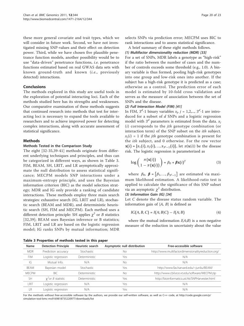
these more general covariate and trait types, which wewill consider in future work. Second, we have not inves-tigated missing SNP-values and their effect on detectionpower. Third, while we have chosen five plausible pene-trance function models, another possibility would be touse “data-driven” penetrance functions, i.e. penetrancefunctions estimated based on real GWAS data sets withknown ground-truth and known (i.e., previouslydetected) interactions.

ConclusionsThe methods explored in this study are useful tools inthe exploration of potential interacting loci. Each of themethods studied here has its strengths and weaknesses.Our comparative examination of these methods suggeststhat continued research into methods that test for inter-acting loci is necessary to expand the tools available toresearchers and to achieve improved power for detectingcomplex interactions, along with accurate assessment ofstatistical significance.

MethodsMethods Tested in the Comparison StudyThe eight [32-35,39-41] methods originate from differ-ent underlying techniques and principles, and thus canbe categorized in different ways, as shown in Table 3.FIM, BEAM, SH, LRIT, and LR asymptotically approxi-mate the null distribution to assess statistical signifi-cance; MECPM models SNP interactions under amaximum-entropy principle, and uses the Bayesianinformation criterion (BIC) as the model selection strat-egy; MDR and IG only provide a ranking of candidateinteractions. These methods employ three main searchstrategies: exhaustive search (IG, LRIT and LR), stochas-tic search (BEAM and MDR), and deterministic heuris-tic search (SH, FIM and MECPM). Each method uses adifferent detection principle: SH applies c2 or B statistics[32,39]; BEAM uses Bayesian inference or B statistics;FIM, LRIT and LR are based on the logistic regressionmodel; IG ranks SNPs by mutual information; MDR

selects SNPs via prediction error; MECPM uses BIC torank interactions and to assess statistical significance.A brief summary of these eight methods follows.

(1) Multifactor dimensionality reduction (MDR) [33]For a set of SNPs, MDR labels a genotype as “high-risk”if the ratio between the number of cases and the num-ber of controls exceeds some threshold (e.g., 1.0). A bin-ary variable is thus formed, pooling high-risk genotypesinto one group and low-risk ones into another. If thesubject has a high-risk genotype it is predicted as a case;otherwise as a control. The prediction error of eachmodel is estimated by 10-fold cross validation andserves as the measure of association between the set ofSNPs and the disease.(2) Full Interaction Model (FIM) [41]In FIM, 3d-1 binary variables xj, j = 1,2,..., 3d-1 are intro-duced for a subset of d SNPs and a logistic regressionmodel with 3d parameters is estimated from the data. xj(i) corresponds to the jth genotype combination (orinteraction term) of the SNP subset on the ith subject.xj(i) = 1 if the jth genotype combination is present forthe ith subject, and 0 otherwise. For the row vectorx(i) = [x1(i), x2(i), ..., x3d−1(i)] , let π(x(i)) be the diseaserisk. The logistic regression is parameterized as

log(

π(x(i))1 − π(x(i))

)= β0 + βx(i)T (3)

where β0, β =[β1, ...,β3d−1

]are estimated via maxi-

mum likelihood estimation. A likelihood-ratio test isapplied to calculate the significance of this SNP subsetvia an asymptotic c2 distribution.(3) Information Gain (IG) [34]Let C denote the disease status random variable. Theinformation gain of {A, B} is defined as

IG(A,B,C) = I(A;B|C) − I(A;B) (4)

where the mutual information I(A;B) is a non-negativemeasure of the reduction in uncertainty about the value

Table 3 Properties of methods tested in this paper

Name Detection Principle Heuristic search Asymptotic null distribution Free-accessible software

MDR Prediction accuracy Stochastic No http://www.multifactordimensionalityreduction.org/

FIM Logistic regression Deterministic Yes N/A

IG Mutual Info. N/A No N/A

BEAM Bayesian model Stochastic Yes http://www.fas.harvard.edu/~junliu/BEAM/

MECPM BIC Deterministic No http://www.cbil.ece.vt.edu/software/MECPM.zip

SH c2or B statistic Deterministic Yes http://bioinformatics.ust.hk/SNPHarvester.html

LRIT Logistic regression N/A Yes N/A

LR Logistic regression N/A Yes N/A

For the methods without free-accessible software by the authors, we provide our self-written software, as well as C++ code, at http://code.google.com/p/simulation-tool-bmc-ms9169818735220977/downloads/list


of 23

http://www.multifactordimensionalityreduction.org/

http://www.fas.harvard.edu/~junliu/BEAM/

http://www.cbil.ece.vt.edu/software/MECPM.zip

http://bioinformatics.ust.hk/SNPHarvester.html



of (SNP locus) random variable A, given knowledge ofrandom variable B [61] Equivalently, it is a measure ofthe statistical dependence between A and B. The condi-tional mutual information I(A;B |C) likewise gives ameasure of the statistical dependence between A and Bgiven that the phenotype random variable, C, is known.The magnitude of IG thus indicates the increased statis-tical dependence between A and B given knowledge ofC, i.e. the strength of an interaction between loci A andB.(4) Bayesian Epistasis Association Mapping (BEAM) [32]Suppose N samples (Nd cases and Nu controls) are gen-otyped at L SNPs. BEAM partitions the L SNPs into 3groups: markers with no association with disease, mar-kers with only main effects, and markers with interac-tion effects. Let the genotypes on cases be D = (d1,...,dL)

with dj =[dj1, ..., djNd

]representing genotype vector of

the jth SNP at all the cases. According to the above-mentioned partitioning, D can be divided into three sub-sets, D0, D1, and D2, where D0 is the subset consisting ofSNPs (SNP genotype vectors) with no association, D1 isthe subset consisting of SNPs with only main effects,and D2 is the subset consisting of SNPs with interactioneffects. Likewise, let the genotypes on controls be U =(u1,...,uL) with uj =

(uj1, ..., ujNu

)representing genotypes

of the jth SNP at the controls. Let I = [I1,I2,..., IL] be themembership of SNPs within each group, e.g. Ij = 0means that the jth SNP has a main effect, Ij = 1 meansthat the jth SNP has only main effects, Ij = 2 means thatthe jth SNP has interaction effects. Let P() be the prob-ability symbol. Following some assumptions [32], theposterior distribution of I given D and U is inferred by:

P(I|D,U)

∝ P(D1|I) · P(D2|I) · P(D0,U|I) · P(I). (5)

Based on equation (5), BEAM draws I using theMetropolis-Hastings algorithm. The output is the pos-terior probability of main-effect markers and interac-tions associated with the disease. A “B“ statistic is alsoapplied to measure statistical significance of SNPs andinteractions.(5) SNP Harvester (SH) [39]This method aims to detect interactions with weak mar-ginal effects. It includes the following steps:5a. Remove SNPs with significant main effects;5b. For a fixed M, run the “PathSeeker” heuristic

search to identify M-way SNP interactions. First, ran-domly select M SNPs to form a M-way set A = {x1,x2,..., xM}. Second, swap one of the remaining SNPs witheach member of A, to see whether a statistical score s(A) (e.g. c2statistic, B statistic) increases. Then iterativelyrepeat this second step until convergence; record s(A) if

statistically significant. Then go back to the first step,with the optimal A removed as a candidate for the nextrun.5c. Use L2-norm penalized logistic regression [37] as a

post processing step to further select interactions fromthose identified in 5b.Although SH removes SNPs with strong main effects,

for purpose of fair comparison, we still give it credit foridentifying these main-effect SNPs in calculating itspower.(6) Maximum entropy conditional probability modeling(MECPM) [40]MECPM builds the phenotype posterior under a maxi-mum entropy principle, encodes constraints into themodel that correspond 1-to-1 to interactions, flexiblyallows dominant or recessive coding for each locus in acandidate interaction, searches interactions via a greedyinteraction growing search strategy that evaluates candi-dates up to fifth order, and uses the Bayesian informa-tion criterion (BIC) as the model selection strategy.(7) Logistic regression (LR) [35]LR is a generalized linear model used for binomialregression. Let x(i) correspond to the genotype of a SNPfor the ith subject. x(i) = 0 denotes homozygous majoralleles; x(i) = 1 denotes heterozygous genotypes; and x(i)= 2 denotes homozygous minor alleles. Let π (x(i)) bethe disease risk. The logistic regression is parameterizedas:

log(

π(x(i))1 − π(x(i))

)= β0 + β1x(i) (6)

, where b0 and b1 are the regression coefficients,learned via maximum likelihood. By a likelihood ratiotest, logistic regression evaluates statistical significancefor each SNP.(8) Logistic regression with interaction term (LRIT) [35]LRIT aims at detecting interaction effects based on thelogistic regression model. Let xm(i) and xn(i) correspondto genotypes of the mth SNP and nth SNPs for the ithsubject, respectively. xm(i) = 0 or xn(i) = 0 denoteshomozygous major alleles; xm(i) = 1 or xn(i) = 1 denotesheterozygous genotypes; and xm(i) = 2 or xn(i) = 2denotes homozygous minor alleles. Let π (xm(i), xn(i)) bethe disease risk. The logistic regression is parameterizedas:

log(

π(xm(i), xn(i))1 − π(xm(i), xn(i))

)= β0 + β1xm(i) + β2xn(i) + β3xm(i) · xn(i) (7)

, where b0, b1, b2, b3 are the regression coefficients,learned via maximum likelihood. By a likelihood ratiotest, logistic regression evaluates the statistical signifi-cance for this pair of SNPs (the statistical significance


of 23

reflects the joint effects of the two individual terms andthe multiplicative term).

Additional material

Additional file 1: Supplementary information: comparative analysisof methods for detecting interactive SNPs. This supplementaryinformation consists of 6 sections: S1. Section S1 presents our theoreticalanalysis of the relationship between association strength, joint effect,main effect, penetrance function, and MAF. This section also providessome theoretical explanations about our experimental results. S2. SectionS2 presents comprehensive power evaluation results of the methods fordifferent interaction models and parameter settings, related to powerdefinition 1. The reproducibility of the methods is also shown by thestandard deviation of power. As an extension of the main text, we alsosummarize our findings and analytical explanations for these results. S3.Section S3 provides ROC curves of the methods based on the wholeground-truth SNP set. These ROC curves illustrate the sensitivity andspecificity for the methods. The reproducibility of the methods is alsoshown by the standard deviation of sensitivity. S4. Section S4 describesin detail how the effect size (odds ratio) is calculated for each interactionmodel. S5. Section S5 analyzes the conservativeness of c2 statisticsapplied by SH and FIM. This analysis partly explains why SH and FIM areconservative. S6. Section S6 gives the empirical relationship betweenpower and the false positive SNP count under a given significancethreshold.

AcknowledgementsThis work was supported in part by the National Institutes of Health(HL090567 to D.M.H. and GM085665 to Y.W.).

Author details1Bradley Department of Electrical and Computer Engineering, VirginiaPolytechnic Institute and State University, Arlington, VA, USA. 2Department ofBiostatistical Sciences, Wake Forest School of Medicine, Winston-Salem, NC,USA. 3Department of Electrical Engineering, The Pennsylvania StateUniversity, University Park, PA, USA. 4Department of Internal Medicine, WakeForest School of Medicine, Winston-Salem, NC, USA.

Authors’ contributionsLC and YW designed the experiment protocols and evaluation measures,conducted the experiments, participated in implementation of the methodsand design of simulation tools, and drafted the manuscript. GYimplemented the conventional (also some advanced) interaction-detectionmethods, and participated in design of the experiments. CL designed thesimulation tools. CL, RG and XY carried out the development of simulationsoftware. DM helped to draft and extensively edited the manuscript. DMand JR implemented MECPM. YW and DH conceived of the study,participated in its design and coordination, and helped draft the paper. Allauthors read and approved the final manuscript.

Received: 25 February 2011 Accepted: 5 July 2011Published: 5 July 2011

References1. Brookes A: Review: the essence of SNPs. Gene 1999, 234:177-186.2. Couzin J, Kaiser J: Genome-wide association. Closing the net on common

disease genes. Science 2007, 316:820-2.3. Hirschhorn J: Genome-wide association studies for common diseases

and complex traits. Nature reviews Genetics 2005, 6:95-108.4. Donnelly P: Progress and challenges in genome-wide association studies

in humans. Nature 2008, 456:728-31.5. Manolio TA, et al: Finding the missing heritability of complex diseases.

Nature 2009, 461:747-53.6. T. W. T. C. C. Consortium: Genome-wide association study of 14,000 cases

of seven common diseases and 3,000 shared controls. Nature 2007,447:661-78.

7. Wang WY, et al: Genome-wide association studies: theoretical andpractical concerns. Nat Rev Genet 2005, 6:109-18.

8. Hardy J, Singleton A: Genomewide association studies and humandisease. N Engl J Med 2009, 360:1759-68.

9. Ku CS, et al: The pursuit of genome-wide association studies: where arewe now? Journal of Human Genetics 2010, 55:195-206.

10. Mohlke KL, et al: Metabolic and cardiovascular traits: an abundance ofrecently identified common genetic variants. Hum Mol Genet 2008, 17:R102-8.

11. Kathiresan S, et al: Polymorphisms associated with cholesterol and risk ofcardiovascular events. N Engl J Med 2008, 358:1240-9.

12. Samani NJ, et al: Genomewide association analysis of coronary arterydisease. N Engl J Med 2007, 357:443-53.

13. McPherson R, et al: A common allele on chromosome 9 associated withcoronary heart disease. Science 2007, 316:1488-91.

14. Tsai FJ, et al: A genome-wide association study identifies susceptibilityvariants for type 2 diabetes in Han Chinese. PLoS Genet 2007, 6:e1000847.

15. Scott LJ, et al: A genome-wide association study of type 2 diabetes inFinns detects multiple susceptibility variants. Science 2007, 316:1341-5.

16. Paterson AD, et al: A genome-wide association study identifies a novelmajor locus for glycemic control in type 1 diabetes, as measured byboth A1C and glucose. Diabetes 2010, 59:539-49.

17. Saxena R, et al: Genome-wide association analysis identifies loci for type2 diabetes and triglyceride levels. Science 2007, 316:1331-6.

18. Freedman BI, et al: Differential effects of MYH9 and APOL1 risk variantson FRMD3 association with diabetic ESRD in African Americans. PLoSGenet 2011.

19. Harley JB, et al: Genome-wide association scan in women with systemiclupus erythematosus identifies susceptibility variants in ITGAM, PXK,KIAA1542 and other loci. Nat Genet 2008, 40:204-10.

20. Harley IT, et al: Genetic susceptibility to SLE: new insights from finemapping and genome-wide association studies. Nat Rev Genet 2009,10:285-90.

21. Crow MK: Collaboration, genetic associations, and lupus erythematosus.N Engl J Med 2008, 358:956-61.

22. Lettre G, Rioux JD: Autoimmune diseases: insights from genome-wideassociation studies. Hum Mol Genet 2008, 17:R116-21.

23. Hussman JP, et al: A noise-reduction GWAS analysis implicates alteredregulation of neurite outgrowth and guidance in autism. Mol Autism2011, 2:1.

24. Easton DF, et al: Genome-wide association study identifies novel breastcancer susceptibility loci. Nature 2007, 447:1087-93.

25. Easton DF, Eeles RA: Genome-wide association studies in cancer. HumanMolecular Genetics 2008, 17:R109-R115.

26. Hunter DJ, et al: A genome-wide association study identifies alleles inFGFR2 associated with risk of sporadic postmenopausal breast cancer.Nat Genet 2007, 39:870-4.

27. Amundadottir L, et al: Genome-wide association study identifies variantsin the ABO locus associated with susceptibility to pancreatic cancer. NatGenet 2009, 41:986-90.

28. Maher B: Personal genomes: The case of the missing heritability. Nature2008, 456:18-21.

29. Cordell H: Detecting gene-gene interactions that underlie humandiseases. Nature reviews Genetics 2009, 10:392-404.

30. Moore JH, et al: Bioinformatics challenges for genome-wide associationstudies. Bioinformatics 2010, 26:445-55.

31. Musani SK, et al: Detection of gene × gene interactions in genome-wideassociation studies of human population data. Hum Hered 2007, 63:67-84.

32. Zhang Y, Liu JS: Bayesian inference of epistatic interactions in case-control studies. Nat Genet 2007, 39:1167-73.

33. Ritchie MD, et al: Multifactor-dimensionality reduction reveals high-orderinteractions among estrogen-metabolism genes in sporadic breastcancer. Am J Hum Genet 2001, 69:138-47.

34. Moore JH, et al: A flexible computational framework for detecting,characterizing, and interpreting statistical patterns of epistasis in geneticstudies of human disease susceptibility. J Theor Biol 2006, 241:252-61.

35. Agresti A: Categorical data analysis. 2 edition. New York: Wiley-Interscience;2002.

36. Kooperberg C, Ruczinski I: Identifying interacting SNPs using Monte Carlologic regression. Genet Epidemiol 2005, 28:157-70.


of 23

http://www.biomedcentral.com/content/supplementary/1471-2164-12-344-S1.DOC

http://www.ncbi.nlm.nih.gov/pubmed/10395891?dopt=Abstract

































































37. Park MY, Hastie T: Penalized logistic regression for detecting geneinteractions. Biostatistics 2008, 9:30-50.

38. G Yu, et al: Detection of complex interactions of multi-locus SNPs,”presented at IEEE Machine Learning for Signal Processing. Cancun,Mexico; 2008.

39. Yang C, et al: SNPHarvester: a filtering-based approach for detectingepistatic interactions in genome-wide association studies. Bioinformatics2009, 25:504-11.

40. Miller DJ, et al: An Algorithm for Learning Maximum Entropy ProbabilityModels of Disease Risk That Efficiently Searches and Sparingly EncodesMultilocus Genomic Interactions. Bioinformatics 2009, 25:2478-2485.

41. Marchini J, et al: Genome-wide strategies for detecting multiple loci thatinfluence complex diseases. Nature Genetics 2005, 37:413-417.

42. Schwender H, Ickstadt K: Identification of SNP interactions using logicregression. Biostatistics 2008, 9:187-198.

43. Yang C, et al: Identifying main effects and epistatic interactions fromlarge-scale SNP data via adaptive group Lasso. BMC Bioinformatics 2010,11(Suppl 1):S18.

44. Breiman L: Random forests. Machine Learning 2001, 45:5-32.45. Wang X, et al: The meaning of interaction. Human Heredity 2010,

70:269-277.46. W Li, Reich J: A complete enumeration and classification of two-locus

disease models. Hum Hered 2000, 50:334-49.47. Szymczak S, et al: Machine learning in genome-wide association studies.

Genet Epidemiol 2009, 33(Suppl 1):S51-7.48. Van Steen K: Travelling the world of gene-gene interactions. Brief

Bioinform 2011, 1-19.49. Garcia-Magarinos M, et al: Evaluating the ability of tree-based methods

and logistic regression for the detection of SNP-SNP interaction. AnnHum Genet 2009, 73:360-9.

50. Motsinger-Reif AA, et al: A comparison of analytical methods for geneticassociation studies. Genet Epidemiol 2008, 32:767-78.

51. Carlborg O, Haley C: Epistatis: too often neglected in complex traitstudies? Nature Reviews Genetics 2004, 5:618-625.

52. Jakulin A, Bratko I: Testing the Significance of Attribute Interactions,”presented at the 21st International Conference on Machine Learning(ICML-2004). Banff, Canada; 2004.

53. Jung HY, et al: New methods for imputation of missing genotype usinglinkage disequilibrium and haplotype information. Information Sciences2007, 177:804-814.

54. Chen L, et al: A Ground Truth Based Comparative Study on DetectingEpistatic SNPs. presented at Proc. IEEE Intl Conf. on Bioinformatics &Biomedicine, Washington D.C., USA 2009.

55. Hochberg Y, Tamhane AC: Multiple comparison procedures New York: Wiley;1987.

56. Neel J: Diabetes mellitus: a “thrifty” genotype rendered detrimental by“progress”. Am J Hum Genet 1962, 14:353-362.

57. Wolf J, et al: Epistasis and the Evolutionary Process New York: OxfordUniversity Press Inc.; 2000.

58. Wright FA, et al: Simulating association studies: a data-based resamplingmethod for candidate regions or whole genome scans. Bioinformatics2007, 23:2581-8.

59. Yuan X, et al: Simulating linkage disequilibrium structures in a humanpopulation for SNP association studies. Biochem Genet 2011, 49:395-409.

60. Cordell H: Epistasis: what it means, what it doesn’t mean, and statisticalmethods to detect it in humans. Human Molecular Genetics 2002,11:2463-2468.

61. Cover TM, Thomas JA: Elements of Information Theory New York City: JohnWiley & Sons, Inc.; 1991.

doi:10.1186/1471-2164-12-344Cite this article as: Chen et al.: Comparative analysis of methods fordetecting interacting loci. BMC Genomics 2011 12:344.

Submit your next manuscript to BioMed Centraland take full advantage of:

• Convenient online submission

• Thorough peer review

• No space constraints or color figure charges

• Immediate publication on acceptance

• Inclusion in PubMed, CAS, Scopus and Google Scholar

• Research which is freely available for redistribution

Submit your manuscript at www.biomedcentral.com/submit


of 23
































METHODOLOGY ARTICLE Open Access Comparative analysis of ... · METHODOLOGY ARTICLE Open Access...

Documents

Transcript of METHODOLOGY ARTICLE Open Access Comparative analysis of ... · METHODOLOGY ARTICLE Open Access...