Method Parameters

Data acquisition parameters

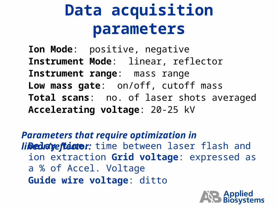
Ion Mode: positive, negativeInstrument Mode: linear, reflectorInstrument range: mass rangeLow mass gate: on/off, cutoff massTotal scans: no. of laser shots averagedAccelerating voltage: 20-25 kV

Delay time: time between laser flash and ion extraction Grid voltage: expressed as a % of Accel. VoltageGuide wire voltage: ditto

Parameters that require optimization in linear/reflector:

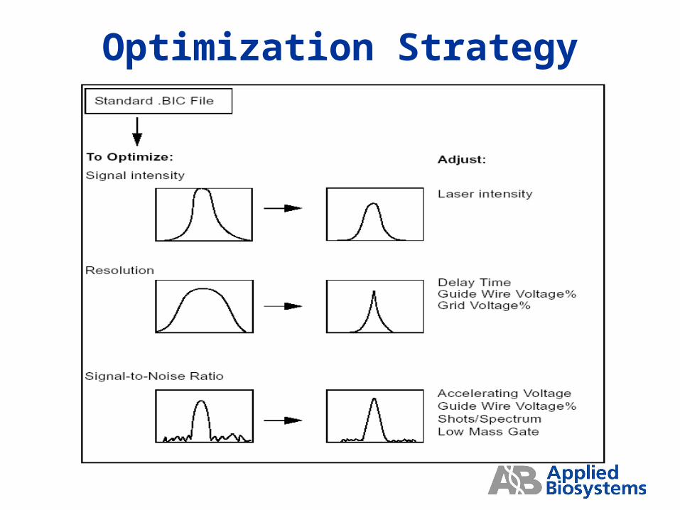
Optimization Strategy

Laser Power

Affects S/N and Resolution

A different power setting will be needed for 3 vs 20 Hz acquisition rate

A different setting is needed for different matrices and sample types

Excessive laser power will result in saturated peaks with poor resolution and high sample consumption

Bin Size(Data Collection Interval)

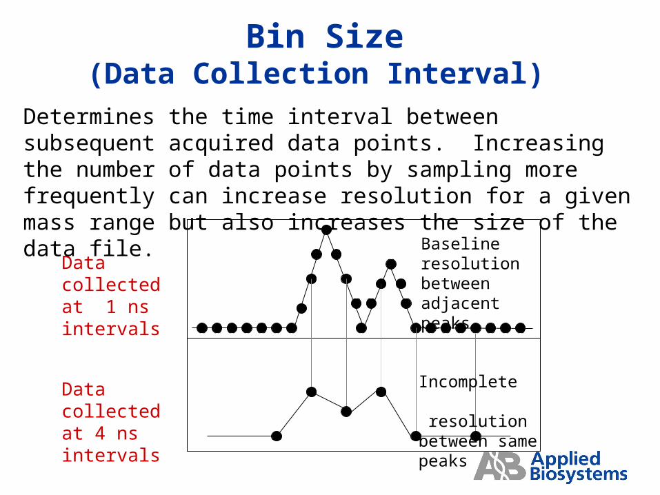
Data collected at 1 ns intervals

Baseline resolution between adjacent peaks.

Incomplete resolution between same peaks

Data collected at 4 ns intervals

Determines the time interval between subsequent acquired data points. Increasing the number of data points by sampling more frequently can increase resolution for a given mass range but also increases the size of the data file.

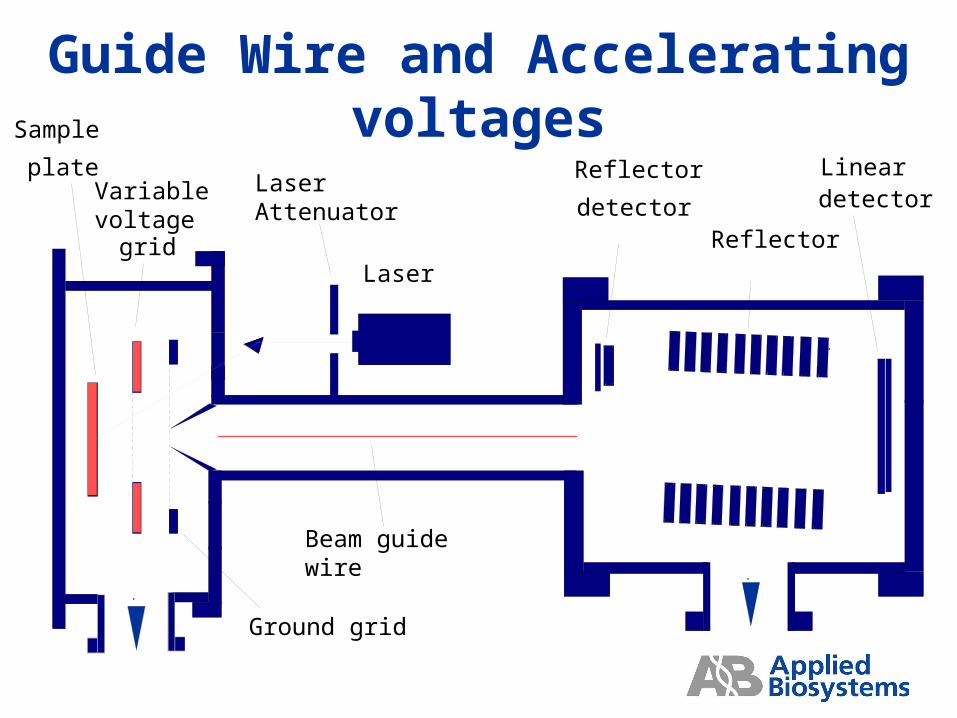
Laser

Sample

plate

Beam guide wire

Reflector

Linear detectorVariable

voltagegrid

Reflector

detectorLaserAttenuator

Ground grid

Guide Wire and Accelerating voltages

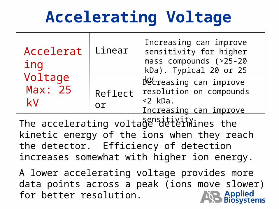
Accelerating Voltage

Accelerating Voltage

Linear

Reflector

Increasing can improve sensitivity for higher mass compounds (>25-20 kDa). Typical 20 or 25 kV.

Decreasing can improve resolution on compounds <2 kDa. Increasing can improve sensitivity

The accelerating voltage determines the kinetic energy of the ions when they reach the detector. Efficiency of detection increases somewhat with higher ion energy.

A lower accelerating voltage provides more data points across a peak (ions move slower) for better resolution.

Max: 25 kV

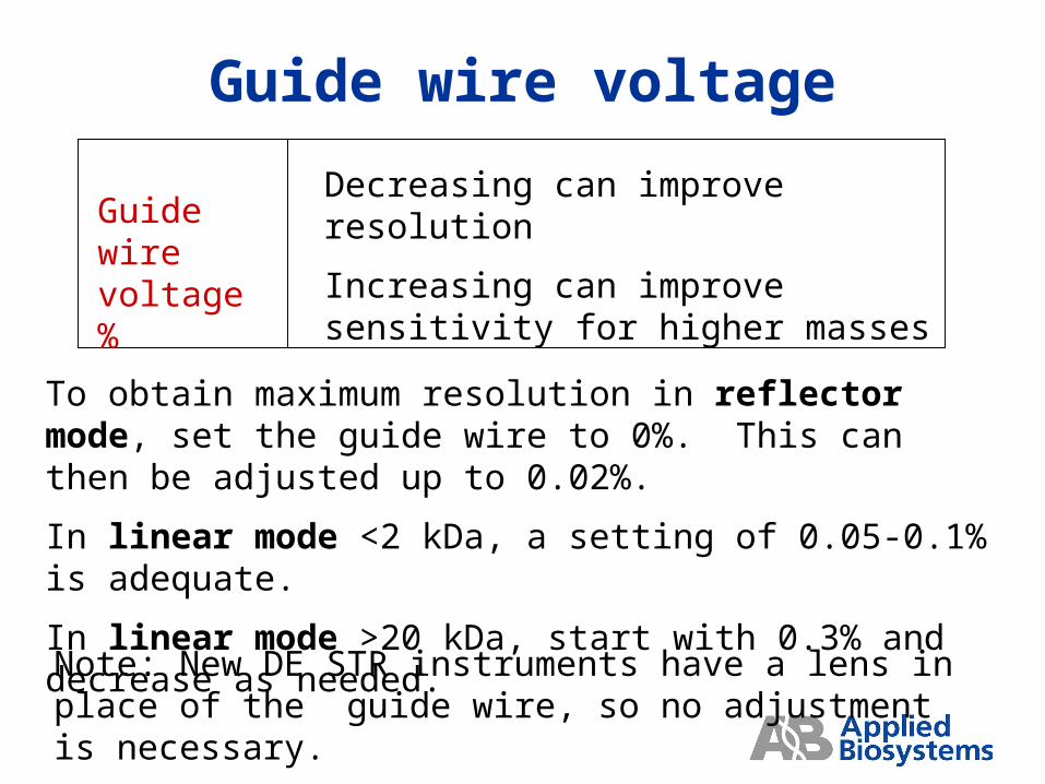
Guide wire voltage

Guide wire voltage %

Decreasing can improve resolution

Increasing can improve sensitivity for higher masses

To obtain maximum resolution in reflector mode, set the guide wire to 0%. This can then be adjusted up to 0.02%.

In linear mode <2 kDa, a setting of 0.05-0.1% is adequate.

In linear mode >20 kDa, start with 0.3% and decrease as needed.

Note: New DE STR instruments have a lens in place of the guide wire, so no adjustment is necessary.

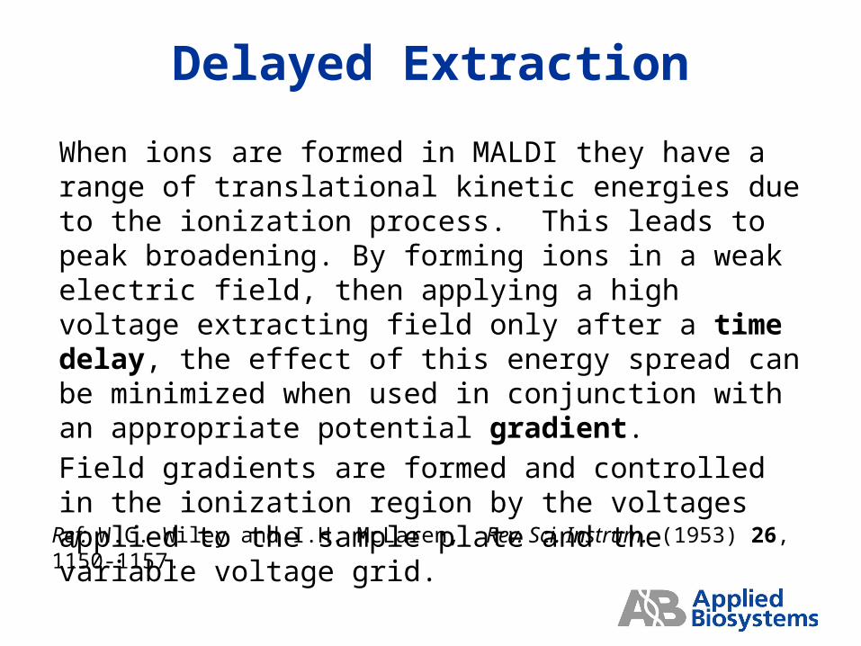
Delayed Extraction

Ref: W.C. Wiley and I.H. McLaren, Rev. Sci. Instrum. (1953) 26, 1150-1157.

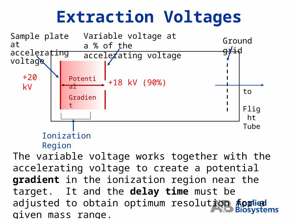
When ions are formed in MALDI they have a range of translational kinetic energies due to the ionization process. This leads to peak broadening. By forming ions in a weak electric field, then applying a high voltage extracting field only after a time delay, the effect of this energy spread can be minimized when used in conjunction with an appropriate potential gradient.

Field gradients are formed and controlled in the ionization region by the voltages applied to the sample plate and the variable voltage grid.

+20 kV+18 kV (90%)Potential

Gradient

Ionization Region

Sample plate at accelerating voltage

Variable voltage at a % of the accelerating voltage

Ground grid

The variable voltage works together with the accelerating voltage to create a potential gradient in the ionization region near the target. It and the delay time must be adjusted to obtain optimum resolution for a given mass range.

to Flight Tube

Extraction Voltages

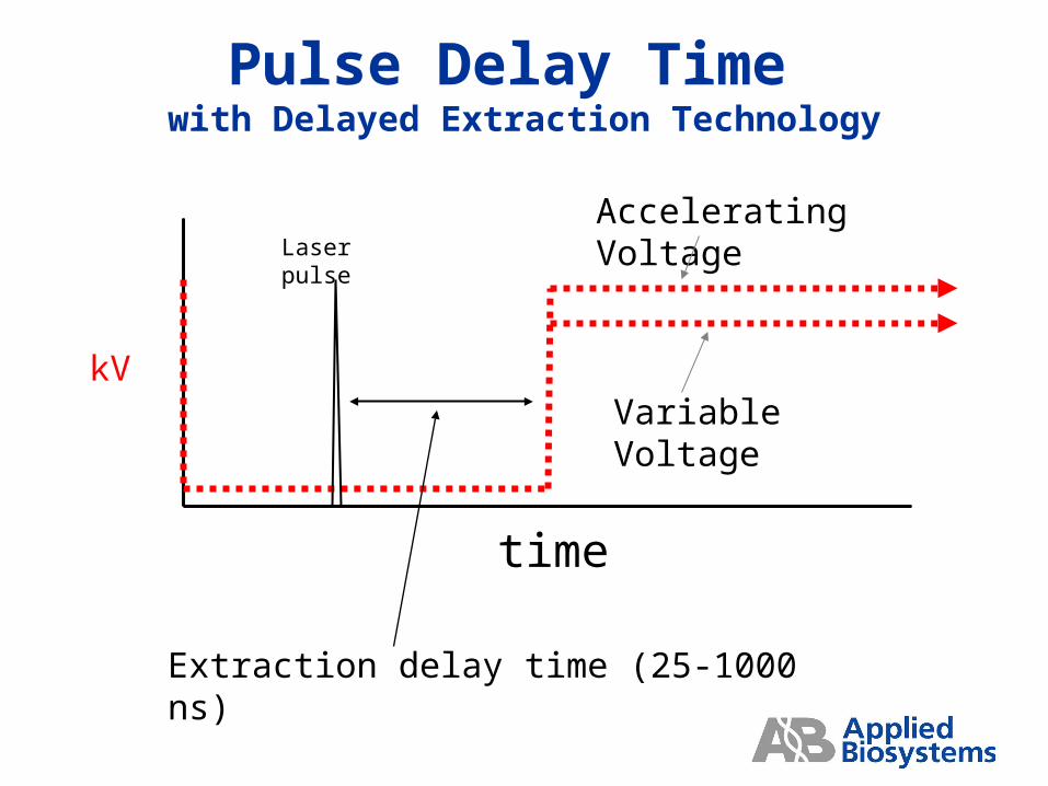
Pulse Delay Time with Delayed Extraction Technology

time

Extraction delay time (25-1000 ns)

Laser pulseAccelerating Voltage

kVVariable Voltage

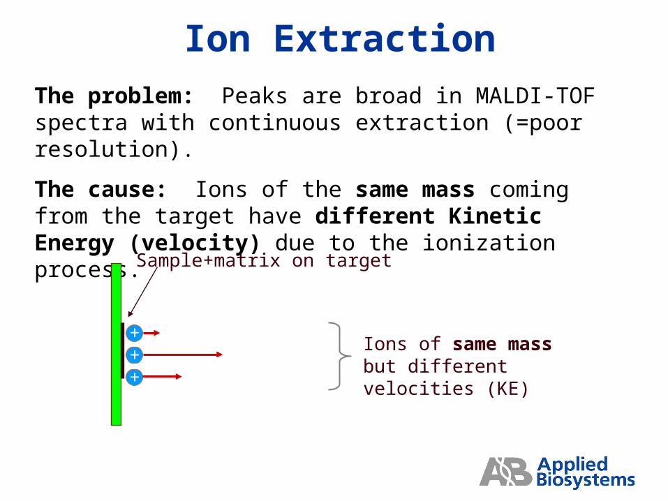
The problem: Peaks are broad in MALDI-TOF spectra with continuous extraction (=poor resolution).

The cause: Ions of the same mass coming from the target have different Kinetic Energy (velocity) due to the ionization process.

+

++

Sample+matrix on target

Ions of same mass but different velocities (KE)

Ion Extraction

+

++

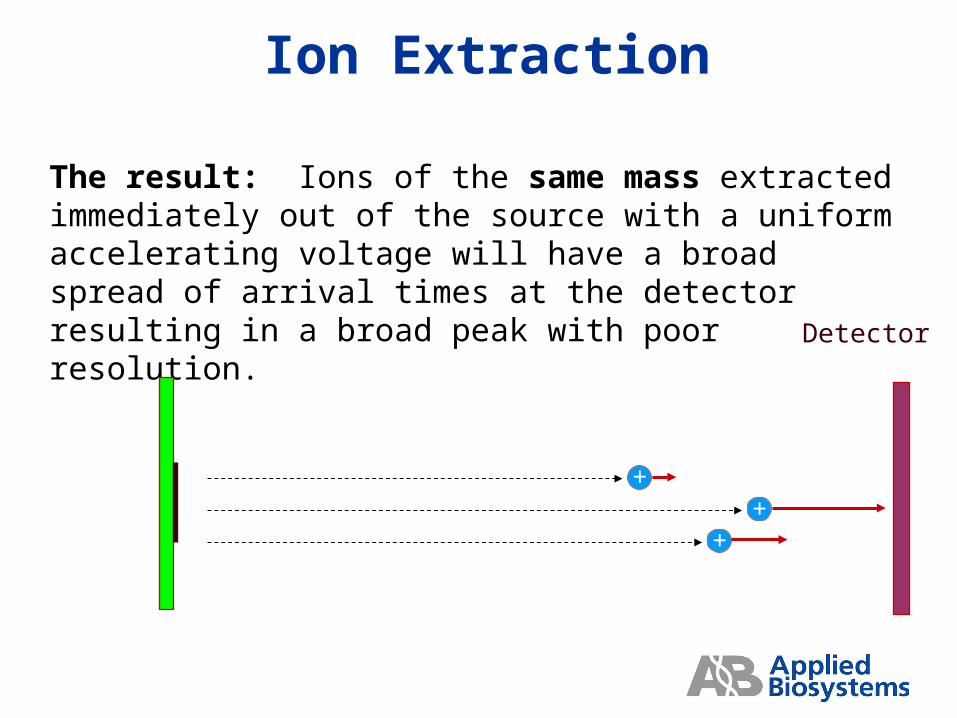
The result: Ions of the same mass extracted immediately out of the source with a uniform accelerating voltage will have a broad spread of arrival times at the detector resulting in a broad peak with poor resolution.

Ion Extraction

Detector

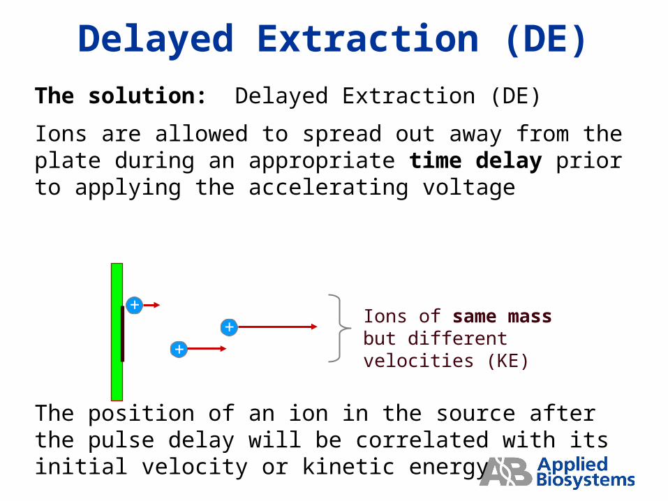
The solution: Delayed Extraction (DE)

Ions are allowed to spread out away from the plate during an appropriate time delay prior to applying the accelerating voltage

Delayed Extraction (DE)

++

+

The position of an ion in the source after the pulse delay will be correlated with its initial velocity or kinetic energy

Ions of same mass but different velocities (KE)

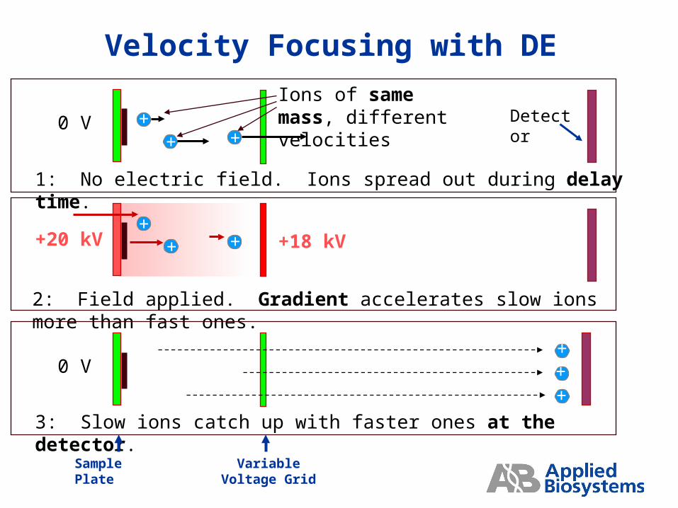
Velocity Focusing with DE

++ +

Ions of same mass, different velocities

1: No electric field. Ions spread out during delay time.

2: Field applied. Gradient accelerates slow ions more than fast ones.

++ +

3: Slow ions catch up with faster ones at the detector.

0 V

+20 kV

0 V

+++

Detector

+18 kV

Sample Plate Variable Voltage Grid

m/z

6130 6140 6150 6160 6170 10600 10800 11000 11200 11400 11600

m/z

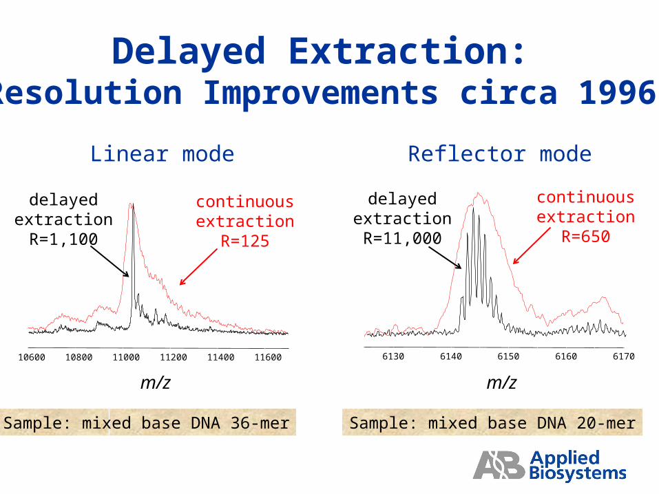
Linear mode Reflector mode

continuousextraction

R=125

delayedextractionR=1,100

delayedextractionR=11,000

continuousextraction

R=650

Delayed Extraction:Resolution Improvements circa 1996

Sample: mixed base DNA 36-mer Sample: mixed base DNA 20-mer

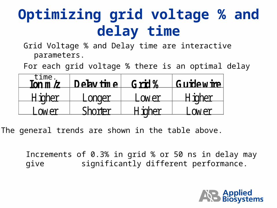
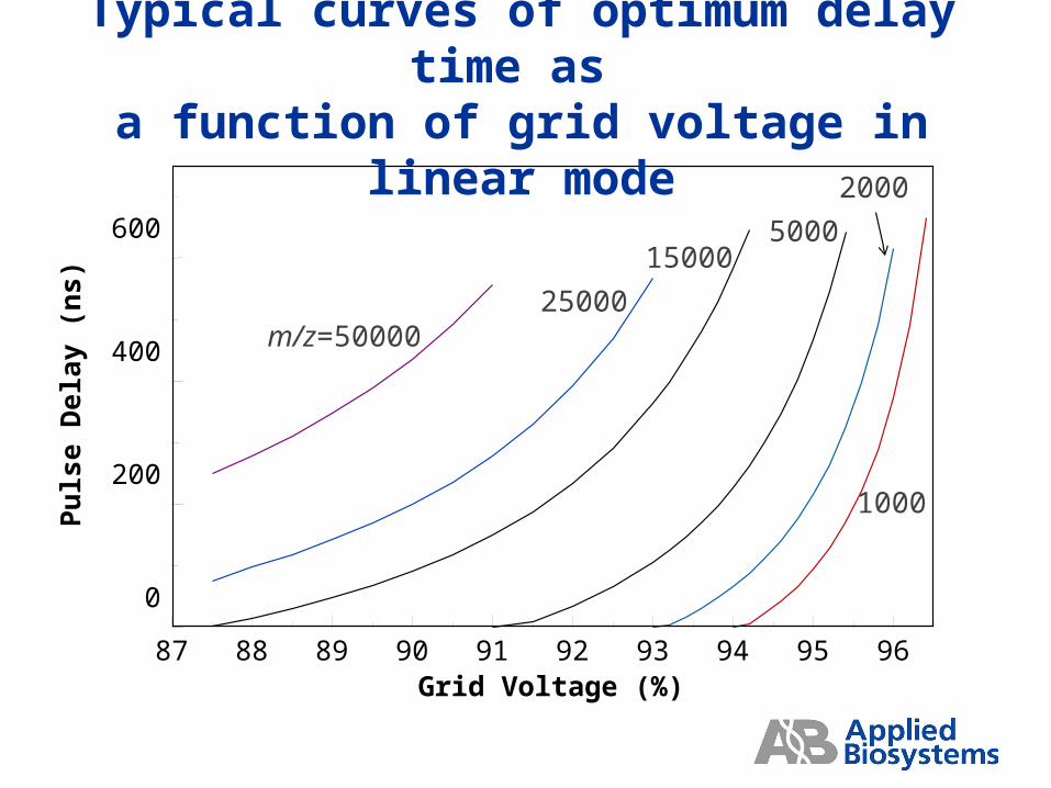
Optimizing grid voltage % and delay time

Grid Voltage % and Delay time are interactive parameters.

For each grid voltage % there is an optimal delay time.

Increments of 0.3% in grid % or 50 ns in delay may give significantly different performance.

Ion m/z Delay time Grid % Guide wireHigher Longer Lower HigherLower Shorter Higher Lower

The general trends are shown in the table above.

0

200

400

600

87 88 89 90 91 92 93 94 95 96Grid Voltage (%)

Pu

lse D

ela

y (

ns)

1000

2000

500015000

25000m/z=50000

Typical curves of optimum delay time as a function of grid voltage in linear mode

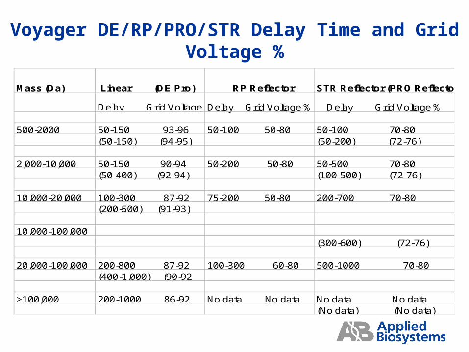
Mass (Da) Linear (DE Pro) RP Reflector STR Reflector (PRO Reflector)

Delay Grid Voltage %Delay Grid Voltage % Delay Grid Voltage %

500-2000 50-150 93-96 50-100 50-80 50-100 70-80(50-150) (94-95) (50-200) (72-76)

2,000-10,000 50-150 90-94 50-200 50-80 50-500 70-80(50-400) (92-94) (100-500) (72-76)

10,000-20,000 100-300 87-92 75-200 50-80 200-700 70-80(200-500) (91-93)

10,000-100,000(300-600) (72-76)

20,000-100,000 200-800 87-92 100-300 60-80 500-1000 70-80(400-1,000) (90-92

>100,000 200-1000 86-92 No data No data No data No data(No data) (No data)

Voyager DE/RP/PRO/STR Delay Time and Grid Voltage %

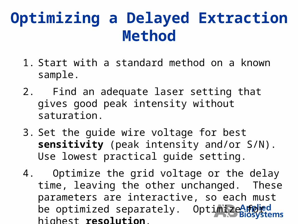
Optimizing a Delayed Extraction Method

1. Start with a standard method on a known sample.

2. Find an adequate laser setting that gives good peak intensity without saturation.

3. Set the guide wire voltage for best sensitivity (peak intensity and/or S/N). Use lowest practical guide setting.

4. Optimize the grid voltage or the delay time, leaving the other unchanged. These parameters are interactive, so each must be optimized separately. Optimize for highest resolution.

5. Recheck 3-4, see if you get same results.

Calibration

Voyager Training Class

Calibration Equations

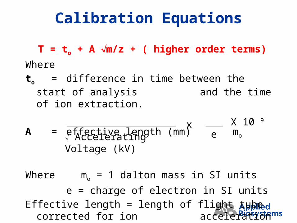
T = to + A m/z + ( higher order terms)

Where

to = difference in time between the start of analysis and the time of ion extraction.

A = effective length (mm) mo

Where mo = 1 dalton mass in SI units

e = charge of electron in SI units

Effective length = length of flight tube corrected for ion acceleration

ex X 10 9

Accelerating Voltage (kV)

Initial Velocity Correction

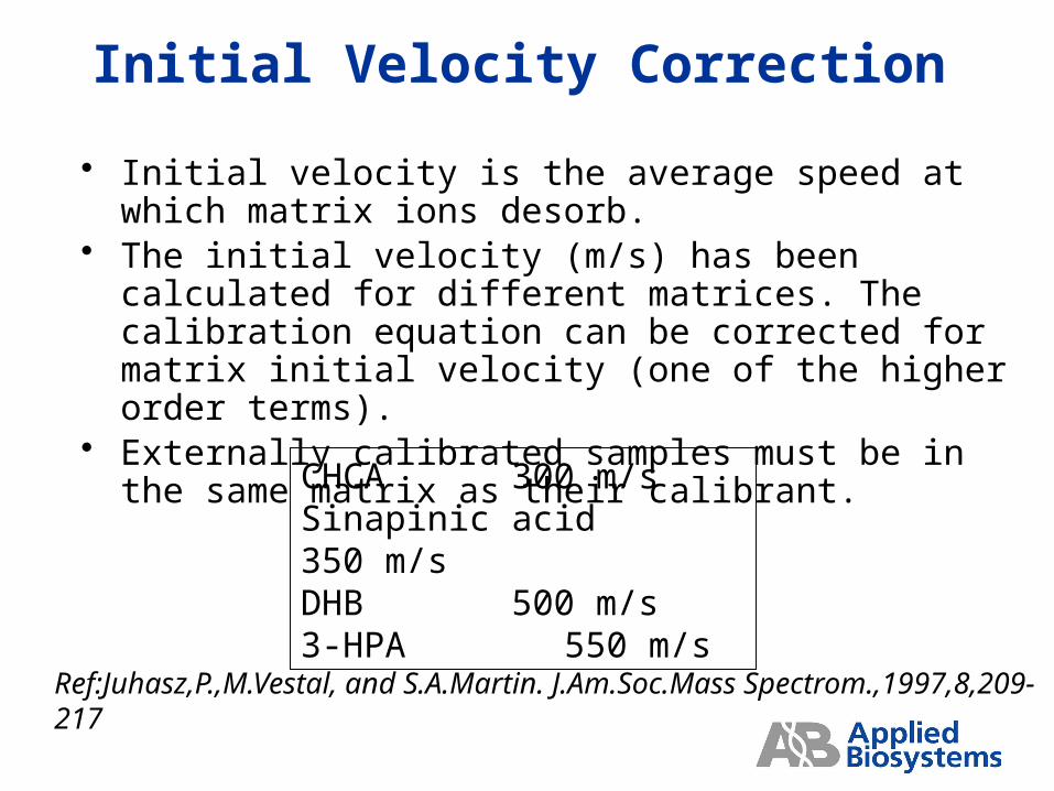
• Initial velocity is the average speed at which matrix ions desorb.

• The initial velocity (m/s) has been calculated for different matrices. The calibration equation can be corrected for matrix initial velocity (one of the higher order terms).

• Externally calibrated samples must be in the same matrix as their calibrant.

CHCA 300 m/sSinapinic acid 350 m/sDHB 500 m/s3-HPA 550 m/s

Ref:Juhasz,P.,M.Vestal, and S.A.Martin. J.Am.Soc.Mass Spectrom.,1997,8,209-217

A default calibration uses a multiparameter equation that estimates values for tº and A from instrument dimensions.

Default calibration is applied to the mass scale if no other calibration is specified.

Calibration Equations

Internal calibration uses a multiparameter equation that calculates values for tº and A using the known mass of the standard(s). This corrects the mass scale.

A multi-point calibration calculates tº and A by doing a least-squares fit to all of the standards.

A two point calibration calculates tº and A from the standards. A one point calibration calculates A from the standard and uses tº from the default calibration.

Calibration Equations

A one-, two- or multi-point calibration using known peak masses that are within the spectrum to be calibrated.

The standards should bracket the mass range of interest. The signal intensities of the standards should be similar to those of the samples.

The calibration equation is saved within the data file and can be exported as a *.cal file to the acquisition method or to another data file.

Internal Calibration

Useful Calibration Standards

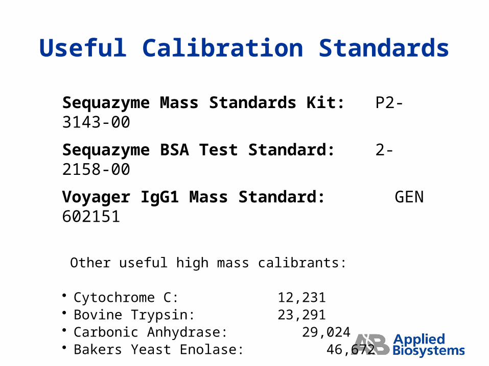
Sequazyme Mass Standards Kit: P2-3143-00

Sequazyme BSA Test Standard: 2-2158-00

Voyager IgG1 Mass Standard: GEN 602151

Other useful high mass calibrants:

• Cytochrome C: 12,231• Bovine Trypsin: 23,291• Carbonic Anhydrase: 29,024• Bakers Yeast Enolase: 46,672

756.4732

807.4383

893.5128

944.4889

1068.6892

1412.8272

1471.7961

1627.9507

1789.8437

1821.9344

1840.9281

1875.9875

1948.0391

2039.14592124.0419 2349.1390

2441.1330

2471.21872583.3076

2973.4467 3178.6034

3187.7327

3490.7970

0

5000

10000

15000

1000 2000 3000

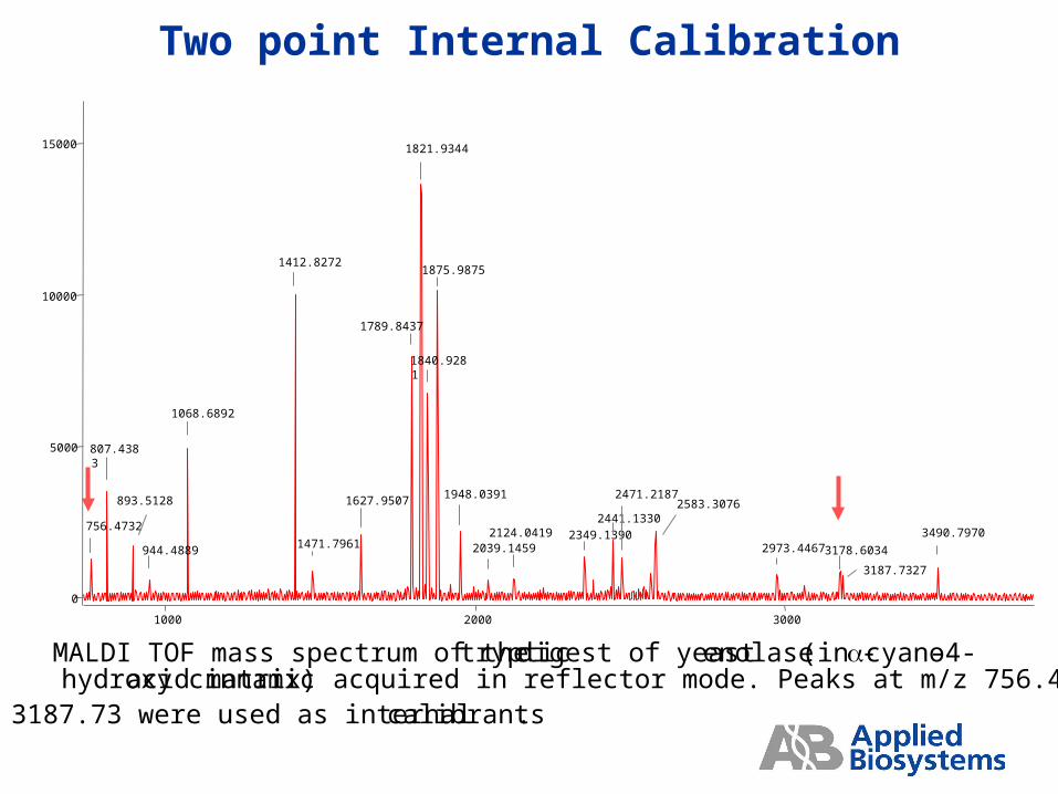
MALDI TOF mass spectrum of the tryptic digest of yeast enolase (in a-cyano-4-hydroxy cinnamic acid matrix) acquired in reflector mode. Peaks at m/z 756.47 and

3187.73 were used as internal calibrants .

Two point Internal Calibration

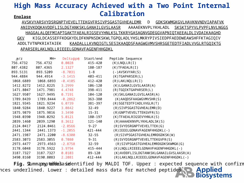
EnolaseAVSKVYARSVYDSRGNPTVEVELTTEKGVFRSIVPSGASTGVHEALEMR DGDKSKWMGKGVLHAVKNVNDVIAPAFVKANIDVKDQKAVDDFLISLDGTANKSKLGANAILGVSLAASR AAAAEKNVPLYKHLADLSKSKTSPYVLPVPFLNVLNGGSHAGGALALQEFMIAPTGAKTFAEALRIGSEVYHNLKSLTKKRYGASAGNVGDEGGVAPNIQTAEEALDLIVDAIKAAGHDGKVKIGLDCASSEFFKDGKYDLDFKNPNSDKSKWLTGPQLADLYHSLMKRYPIVSIEDPFAEDDWEAWSHFFKTAGIQIVADDLTVTNPKRIATAIEK KAADALLLKVNQIGTLSESIKAAQDSFAAGWGVMVSHRSGETEDTFIADLVVGLRTGQIKTGAPARSERLAKLNQLLRIEEELGDNAVFAGENFHHGDKL

m/z MH+ Delta(ppm) Start/end Peptide Sequence756.4732 756.4732 0.0028 415-420 (K)LNQLLR(I)807.4382 807.4365 2.1327 180-187 (K)TFAEALR(I)893.5131 893.5209 -8.7031 1-8 (-)AVSKVYAR(S)944.4884 944.4914 -3.1415 403-411 (K)TGAPARSER(L)1068.6889 1068.6893 -0.4105 412-420 (R)LAKLNQLLR(I)1412.8272 1412.8225 3.2999 106-120 (K)LGANAILGVSLAASR(A)1471.8047 1471.7981 4.4748 398-411 (R)TGQIKTGAPARSER(L)1627.9507 1627.9495 0.7191 104-120 (K)SKLGANAILGVSLAASR(A)1789.8439 1789.8444 -0.2862 363-380 (K)AAQDSFAAGWGVMVSHR(S)1821.9345 1821.9234 6.0739 381-397 (R)SGETEDTFIADLVVGLR(T)1840.9284 1840.9227 3.0842 32-49 (R)SIVPSGASTGVHEALEMR(D)1875.9879 1875.9816 3.3490 15-31 (R)GNPTVEVELTTEKGVFR(S)1948.0390 1948.0292 5.0121 180-197 (K)TFAEALRIGSEVYHNLK(S)2039.1460 2039.1290 8.3612 121-140 (R)AAAAEKNVPLYKHLADLSK(S)2124.0417 2124.0461 -2.0566 9-27 (R)SVYDSRGNPTVEVELTTEK(G)2441.1344 2441.1373 -1.2055 421-444 (R)IEEELGDNAVFAGENFHHGDKL(-)2471.1987 2471.2200 -8.6300 32-55 (R)SIVPSGASTGVHEALEMRDGDKSK(W)2583.3073 2583.3055 0.7080 9-31 (R)SVYDSRGNPTVEVELTTEKGVFR(S)2973.4477 2973.4563 -2.8758 32-59 (R)SIVPSGASTGVHEALEMRDGDKSKWMGK(G)3178.6048 3178.5922 3.9794 415-444 (K)LNQLLRIEEELGDNAVFAGENFHHGDKL(-)3187.7327 3187.7327 0.0103 89-120 (K)AVDDFLISLDGTANKSKLGANAILGVSLAASR(A)3490.8160 3190.8083 2.2081 412-444 (R)LAKLNQLLRIEEELGDNAVFAGENFHHGDKL(-)

Fig. 2 Summary of enolase peptides identified by MALDI TOF. Upper : expected sequence with confirmedsequences underlined. Lower : detailed mass data for matched peptides.

High Mass Accuracy Achieved with a Two Point Internal Calibration

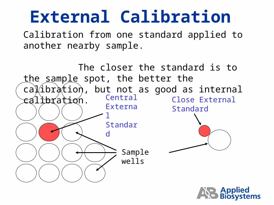
External CalibrationCalibration from one standard applied to another nearby sample. The closer the standard is to the sample spot, the better the calibration, but not as good as internal calibration.

Central External Standard

Sample wells

Close External Standard

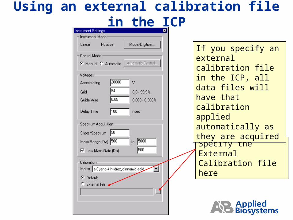
Using an external calibration file in the ICP

Specify the External Calibration file here

If you specify an external calibration file in the ICP, all data files will have that calibration applied automatically as they are acquired

Voyager Instrument

Control Panel

Voyager Training Class

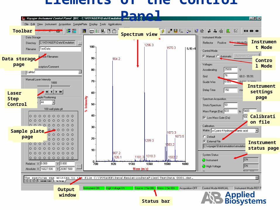
Data storagepage

Sample platepage

Toolbar

Status bar

Spectrum view

Instrumentsettings page

Instrumentstatus page

Output window

Elements of the Control Panel

Calibration file

Instrument Mode

Laser Step Control

Control Mode

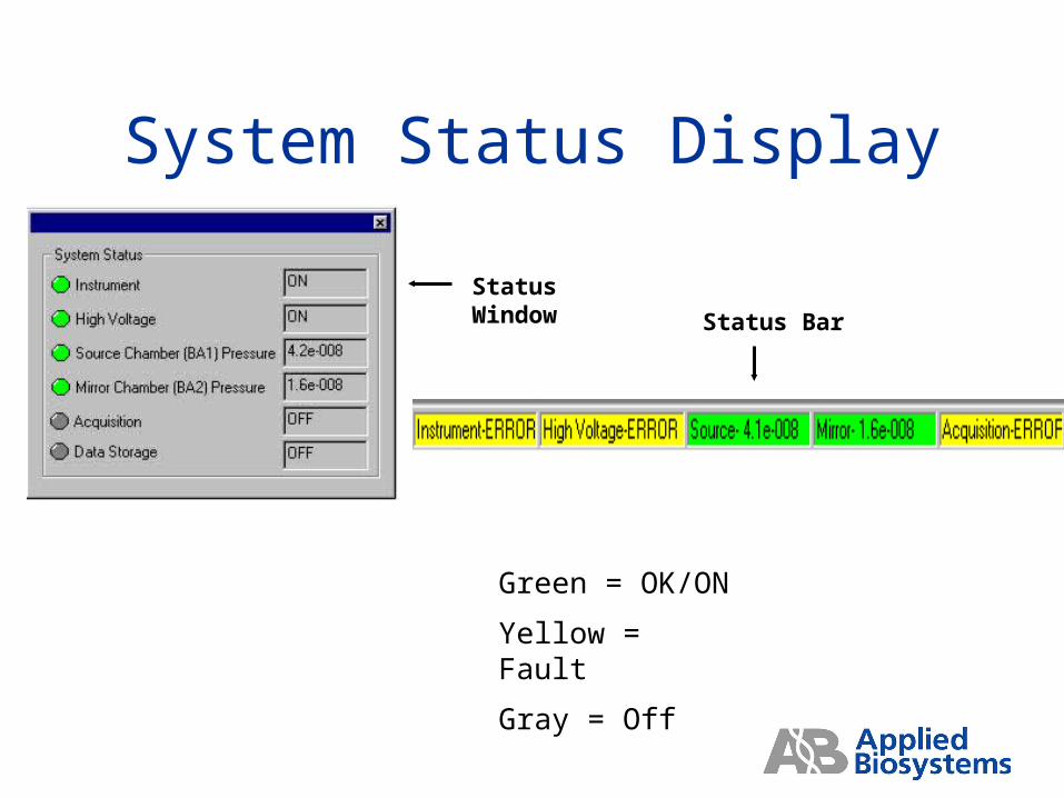
System Status Display

Green = OK/ON

Yellow = Fault

Gray = Off

Status Window

Status Bar

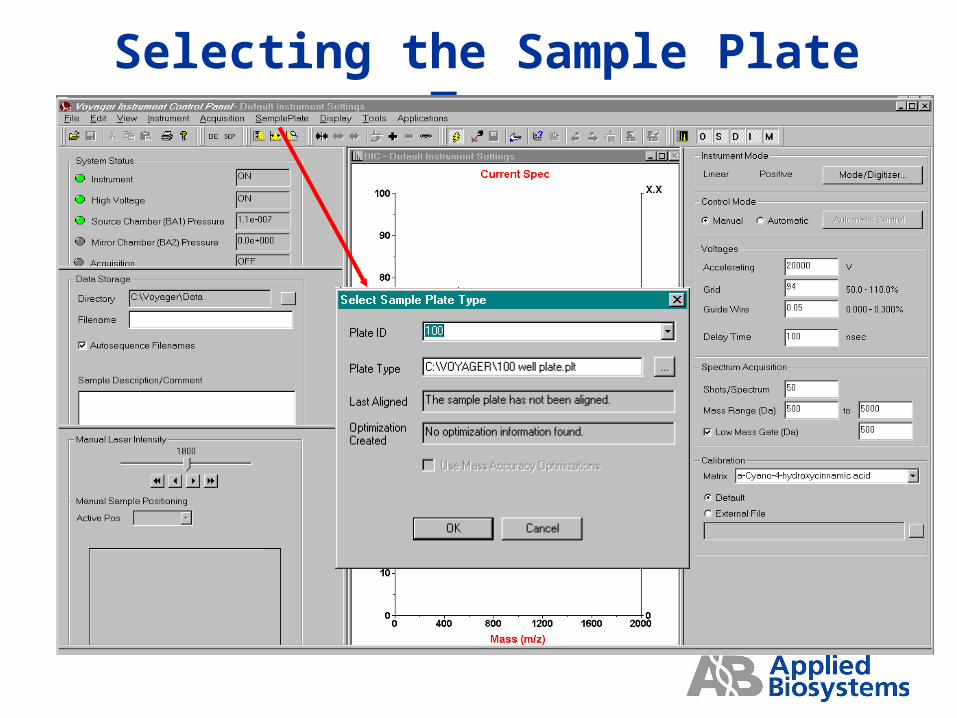
Selecting the Sample Plate Type

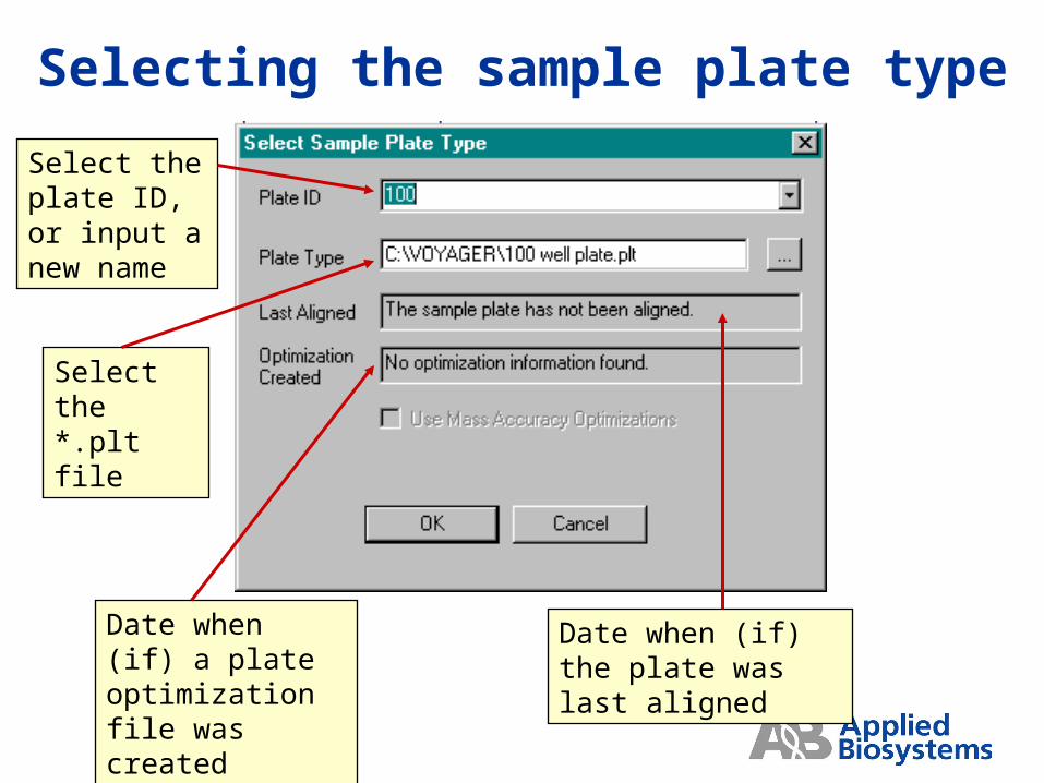
Select the plate ID, or input a new name

Select the *.plt file

Date when (if) the plate was last aligned

Selecting the sample plate type

Date when (if) a plate optimization file was created

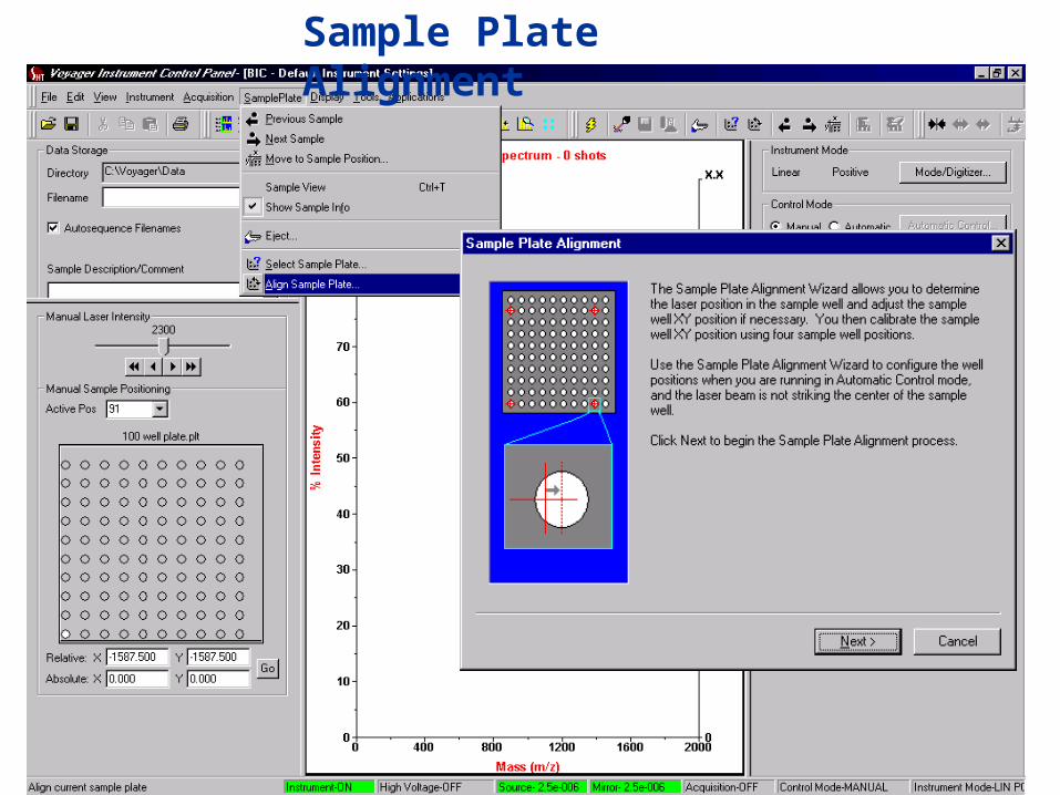
Sample Plate Alignment

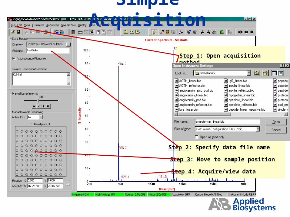
Step 1: Open acquisition method

Step 2: Specify data file name

Step 3: Move to sample position

Step 4: Acquire/view data

Simple Acquisition

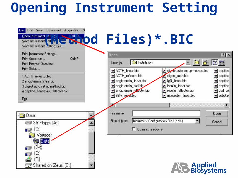
Opening Instrument Setting (Method Files)*.BIC

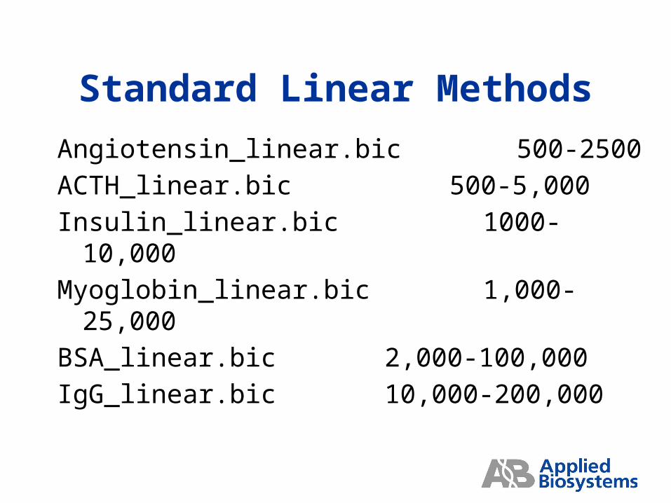
Standard Linear Methods

Angiotensin_linear.bic 500-2500

ACTH_linear.bic 500-5,000

Insulin_linear.bic 1000-10,000

Myoglobin_linear.bic 1,000-25,000

BSA_linear.bic 2,000-100,000

IgG_linear.bic 10,000-200,000

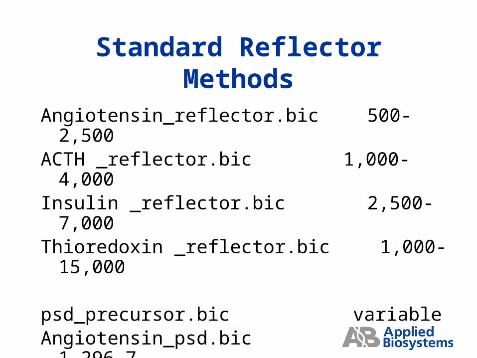
Standard Reflector Methods

Angiotensin_reflector.bic 500-2,500ACTH _reflector.bic 1,000-4,000Insulin _reflector.bic 2,500-7,000Thioredoxin _reflector.bic 1,000-15,000

psd_precursor.bic variableAngiotensin_psd.bic 1,296.7Angiotensin_auto psd.bic 1,296.7

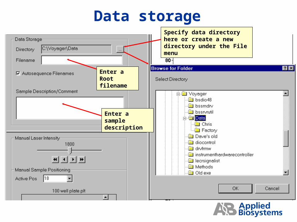
Data storage

Enter a Root filename

Enter a sample description

Specify data directory here or create a new directory under the File menu

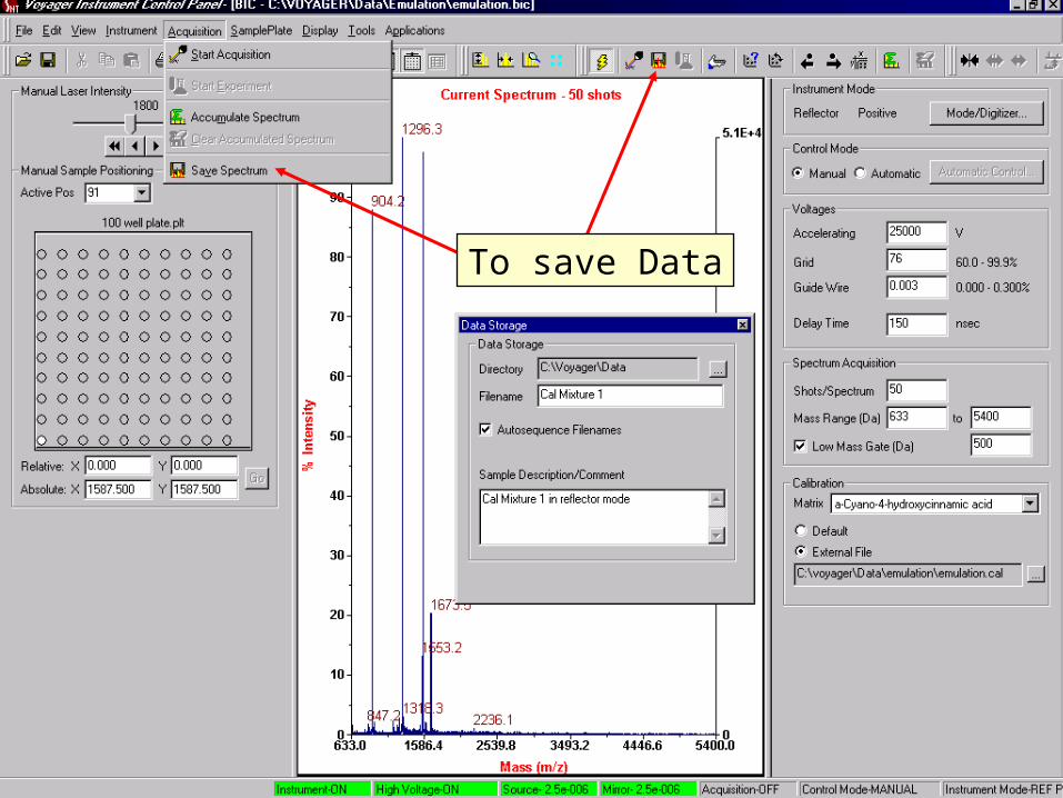
To save Data

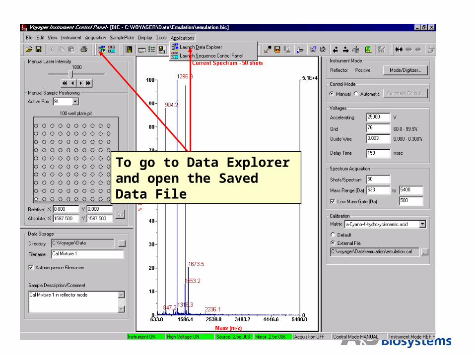
To go to Data Explorer and open the Saved Data File

Laser power setting

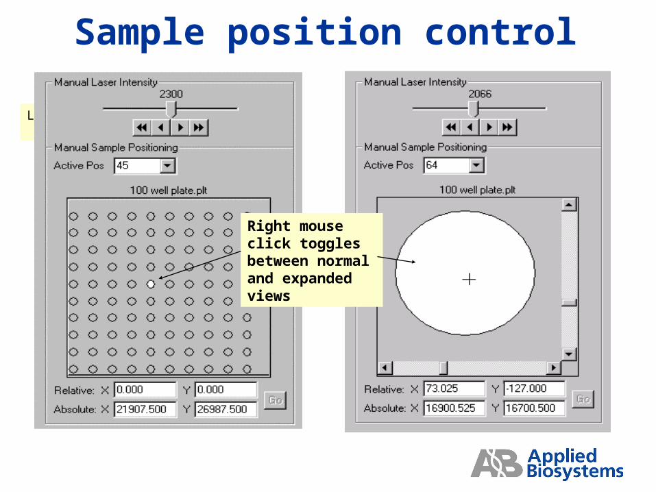
Sample position control

Right mouse click toggles between normal and expanded views

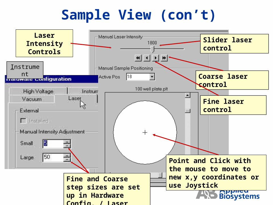
Sample View (con’t)Laser Intensity

Controls

Point and Click with the mouse to move to new x,y coordinates or use Joystick

Coarse laser control

Slider laser control

Fine laser control

Fine and Coarse step sizes are set up in Hardware Config. / Laser

Instrument

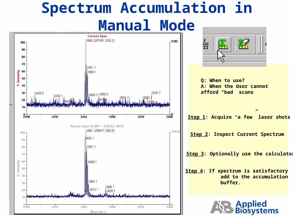
Step 1: Acquire “a few” laser shots

Step 2: Inspect Current Spectrum

Step 3: Optionally use the calculators

Step 4: If spectrum is satisfactory add to the accumulation buffer.

Q: When to use?A: When the user cannot afford “bad” scans

Spectrum Accumulation in Manual Mode

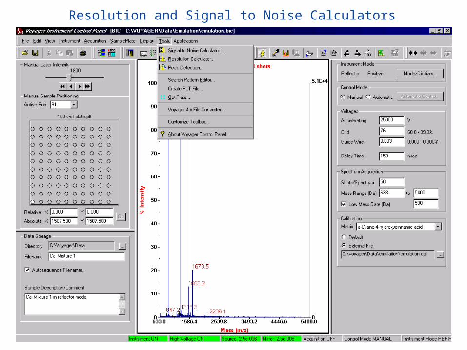
Resolution and Signal to Noise Calculators

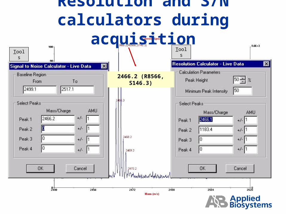
Resolution and S/N calculators during acquisition

2466.2 (R8566, S146.3)

Tools Tools

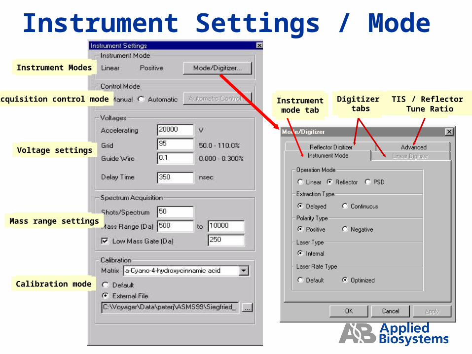
Instrumentmode tab

Digitizer tabs

TIS / Reflector Tune Ratio

Instrument Modes

Voltage settings

Acquisition control mode

Mass range settings

Calibration mode

Instrument Settings / Mode

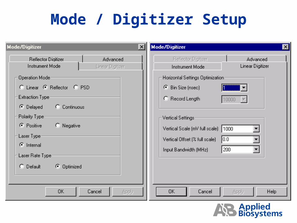
Mode / Digitizer Setup

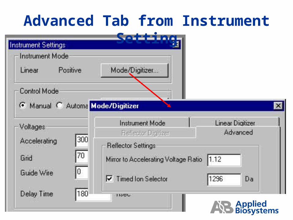
Advanced Tab from Instrument Setting

Standard Voyager Acquisition Methods 

The following pages contain details of the standard methods (*.bic files) for Voyager DE, DE-PRO and DE-STR. These files are usually found in the C drive of the Voyager computer in Voyager/Data/Installation. The instrument settings shown in these tables are only starting points and may be different than the actual settings required to achieve a given specification. The GridVoltage % and Guide Wire % settings are the most critical for method optimization.  The settings required to optimize any method varies from one instrument to the next, thus a .bic file copied from another instrument will not necessarily work well on yours without additional fine-tuning.  Keep at least one copy of your optimized .bic files in a write-protected folder. Create a working copy of these files for daily use.