Method for Identifying Models of Nonlinear Systems Using ...

Prepublication Manuscript for MSSP Sracic and Allen of 35

Method for Identifying Models of Nonlinear Systems Using Linear

Time Periodic Approximations

Michael W. Sracic1 and Matthew S. Allen

Department of Engineering Physics

University of Wisconsin-Madison

534 Engineering Research Building

1500 Engineering Drive

Madison, WI 53706

1Corresponding Author: Email: [email protected], Tel: 608-332-0985 (US), Fax: 608-263-7451 (US)

Abstract:

This work presents a new method for identifying models of nonlinear systems from experimental

measurements. The system is first forced to oscillate in stable periodic orbit, and then a small impulsive

disturbance force is used to perturb the system slightly from that orbit. One then measures the response

until the system returns to the periodic orbit. If the nonlinearities in the system are sufficiently smooth and

the perturbation from the periodic orbit is sufficiently small, then one can linearize the perturbed response

about the periodic orbit and approximate the system as linear time periodic. One of a variety of methods

can then be used to extract the time varying modal model of the system from the response. The

extracted modes can be used to construct a time periodic state transition matrix and state coefficient

matrix, which describe the system’s nonlinear dynamics over a range of the states. The resulting model

for the nonlinear system encompasses that portion of the state space that is traversed by the system

during its periodic orbit.

Keywords: Floquet, restoring force, Fourier Series expansion


1. Introduction

The methods used for identifying models of linear systems are quite mature, but many systems

are inherently nonlinear. In some situations, one can use linear theory to adequately approximate the

nonlinear system. However, linear theory cannot correctly describe some important phenomena that are

exhibited by nonlinear systems. For example, the flutter of airfoils due to aeroelastic effects [1] can lead

to nonlinear hardening of jet engine-to-pylon connections causing catastrophic failure [2]. Likewise, when

torque free satellites perform in-space attitude maneuvers they may respond unpredictably and

uncontrollably (chaotically), a cataclysmic nonlinear phenomenon [3]. Power systems may exhibit strong

voltage variability causing abrupt changes in nonlinear system dynamics (bifurcations) and potentially

leading to systemic blackout [4]. These nonlinear phenomena cannot be predicted with linear theory or

by linearly derived models. Nonlinear models must be used to correctly predict the behavior of such

systems.

Many nonlinear systems are difficult to accurately model from first principles, so one would hope

to characterize the system experimentally instead. Various nonlinear system identification methods have

emerged to attempt to extract mathematical models of nonlinear systems from measurements [2].

However, with current methods it is difficult to extract meaningful information from measurements if the

nonlinear system’s order is high or if the form of the nonlinearities is not known a priori. For example, the

Restoring Force Surface method and the Hilbert Transform are both effective time domain techniques for

single degree of freedom systems with relatively complicated nonlinearities. A few variations of these

methods have been proposed for multiple degree of freedom systems, but several difficulties have been

encountered. Other techniques have been found to work well for multiple degree of freedom systems so

long as one can assume a reasonable form for the nonlinearities in the system a priori. Notable

examples include Nonlinear Auto-Regressive Moving Average with eXogeneous input (NARMAX) and

Nonlinear Subspace Identification [5], two time domain methods, and the Conditioned Reverse Path and

Nonlinear Identification through Feedback of the Output (NIFO), two frequency domain methods. More

information can be found on these and other techniques in a few recent review papers [2, 6, 7].

This work presents a new frequency domain method that overcomes some of these limitations.

The method does not require one to guess the mathematical form of the system’s nonlinearities a priori


and it is potentially applicable to relatively high order systems. The method is based on a linearization of

the system of interest along a periodic trajectory. Specifically, suppose that the system of interest

exhibits a stable periodic limit cycle. (In an experiment such a limit cycle might be obtained by driving the

system periodically with an electromagnetic shaker.) As elaborated in the following section, if the

nonlinearities in the system are differentiable all along the periodic orbit, then one could expand the

equations of motion in a Taylor series at each point along the orbit and obtain linearized equations of

motion at each point. Since the orbit is periodic, the parameters in the linearization will vary periodically

with time. The resulting linear time periodic (LTP) model will accurately describe the system’s response

so long as it stays sufficiently close to the periodic orbit [8], and if this is the case then linear system

identification techniques can be used to identify a linearized model of the system.

Figure 1 outlines the proposed approach. The system of interest is assumed to be oscillating in a

stable periodic orbit. A small perturbation is then applied causing response to deviate somewhat from its

periodic orbit, but since the orbit is stable the response of the system eventually returns to the periodic

orbit once again. The response of the system is recorded as it returns to the orbit and this perturbation is

the primary data used to perform system identification. Since perturbations from the periodic orbit can be

modeled using a linear time periodic system model, experimental identification techniques for linear time

periodic systems are used to extract the time-periodic modes of the system from the measurements. In

this work, the lifting method [9] is used together with the frequency domain Algorithm of Mode Isolation

(AMI) [10] for this purpose. For some systems the Stochastic Subspace system identification (SSI)

method [11] may be preferred instead of AMI, so this approach is also explored here and found to give

similar results. Once the time-periodic modes have been estimated, the state transition matrix and state

coefficient matrix of the linear time periodic system can be reconstructed, as described in a recent work

by Allen [9]. Because the system was linearized about the entire nonlinear periodic orbit, the resulting

state matrix describes the nonlinearities at each point in the state space that was visited during the

periodic orbit. This model can then be integrated to directly estimate the nonlinear functions that

comprise the equations of motion over that region of the state space. These nonlinear functions describe,

for example, the nonlinear force-displacement relationships between the different nodes in the system.


Figure 1: Overview of the proposed nonlinear system identification technique.

The rest of this paper is organized as follows. First, the underlying nonlinear systems theory will

be reviewed to elucidate the proposed method. Then, linear time periodic system identification will be

reviewed to explain how to interpret the measurements and extract the linearized time periodic model of

the system. The proposed method will then be demonstrated in Section 3 by applying it to simulated

measurements of a Duffing oscillator excited in various periodic orbits. The results are discussed and the

conclusions summarized in Section 4.

2. Theory

A nonlinear dynamical system with state vector nx is governed by the following differential

equation where f is a nonlinear function defined on an open subset of n that contains all the possible

positions and velocities of the system. The nonlinear function f describes how the state vector, the inputs,

( ) pu t , and time combine to influence the motion of the system.

, ,x f x t u (1)

In experiment, one usually measures a subset of the total states, and those measured responses

( ) qy t can be considered to be an algebraic function of the states, time and the input.

, ,y g x t u (2)

The vector fields f and g generate flows ( , ) ntX x u and ( , ) n

tY x u that can be considered

Lifting+AMI (or other method such as SSI)

Interpret: FSE Method

Construct LTP system

model, Φ(t,t0), A(t),

etc..

Periodic Orbit

Perturbed Response

Approximate LTP System

Extract LTP Modes

Construct LTP Model

Construct NL Model

x

f(x)


as families of solutions of the differential equation [12] for a certain input u. A single solution curve is

defined by its state vector at the initial instant, x0, and by tracing the flow 0( , )tX x u for a finite time from t0.

Many important nonlinear systems inherently exhibit purely or nearly purely periodic motion, such

as a helicopter rotor spinning at a constant rate, a wind turbine [13], or a human walking periodically [14-

16]. Many other nonlinear systems can be driven with a harmonic forcing function to respond in a

periodic orbit. When the motion can be accurately described as periodic with period T, then the flow

contains a periodic orbit and ( ) ( )x t T x t for any state x . If an input is present, then

( ) ( )u t T u t .

If a small disturbance is introduced to the system, such as by an input ( ) ( ) ( )u t u t u t , then

the state of the system, which previously was contained on the periodic orbit, may deviate from that orbit

as ( ) ( ) ( )x t x t x t . Now suppose that f and g are C1 (at least one-time continuously differentiable)

nonlinear functions. Then the system can be linearized about the periodic orbit by expanding Eqs. (1) and

(2) in a Taylor series and neglecting higher order terms.

i j i j

x u

i j i jx u

x f dx x f du u

y g dx x g du u

(3)

The shorthand notation i jf x is used for the Jacobian matrix meaning that the component

in the ith-row and jth-column is the partial derivative of the ith component of f with respect to the jth

component of x. These equations give a linearized model for the system that is valid as long as the

perturbation ( , )x u is sufficiently small and the nonlinearities of the system are sufficiently smooth. This

linearized model can be written as a standard, linear time-varying (time-periodic) state space system

model with

( ) , ( ) ,

( ) , ( )

ij i j ij i jx u

ij i j ij i jx u

A t f x B t f u

C t g x D t g u

. (4)


This model governs the dynamics of the system about the periodic orbit. This work focuses on the case

where the only input applied is ( )u t , which keeps the system in the periodic orbit, so ( ) 0u t . The

response about the periodic trajectory, ( )x t , can then be described using the state transition matrix

0( , )t t .

0 0( ) ( , ) ( )x t t t x t (5)

If the eigenvectors of 0( , )t t are distinct and hence 0( , )t t is diagonalizable, its state

transition matrix can be represented using Floquet theory [9, 17-19] in summation form as

00

1

T

0

( )( , ) ( )

( ) ( ) ( )

rn

rr

r rr

t tt t R t e

R t t t

(6)

where n is the order of the system and ( )r

R t is the rth residue matrix corresponding to the rth Floquet

exponent r and is composed of the product of the rth time periodic right Floquet eigenvector ( )r t and

rth constant left Floquet eigenvector 0( )r

t . These modal parameters, r , ( )r t and 0( )r

t , allow

one to understand and reconstruct the time periodic system, so these are the parameters that we seek to

extract from measurements. Allen suggested two techniques for extracting these parameters from the

frequency spectrum of the free response ( )x t . The first is called the Fourier Series Expansion technique

and the second is called the Lifting technique. The methods are briefly summarized here; further details

can be found in [9].

2.1. Fourier Series Expansion technique

The residue matrix ( )r

R t in the previous equation is periodic because it is proportional to one

of the periodic Floquet eigenvectors, ( )r

t , so it can be expanded in a Fourier series. After expanding

each of the residue matrices in a Fourier series, the state transition matrix can be written as


0

01

( )( )( , )

B

B

Nn

m rr m N

r Tim t t

t t B e

(7)

where m rB is the mth Fourier coefficient matrix of the rth mode and 2T T is the period frequency.

To be exact, the Fourier expansion may require an infinite number of terms, but in practice a finite

number of Fourier terms, m=-NB,…,NB, will provide sufficient accuracy [9, 20]. The equation above

reveals that the free response of the time periodic system consists of n*(2*NB+1) complex exponential

components r Tim . In the frequency domain each of these complex exponential terms gives rise to

a peak in the spectrum, just as each underdamped mode in a linear time invariant (LTI) system gives rise

to a peak in the spectrum. So, the time periodic system appears to have n*(2*NB+1) modes when it

actually has only n. Once one understands this, one can inspect the frequency spectra of a time periodic

system and determine which peaks correspond to each of the modes. Certain peaks will stand out above

the noise depending on the magnitude of the corresponding coefficient m rB . This method can be used

to construct each of the periodic mode vectors, but in practice it requires quite a bit of user intervention so

the Lifting technique is usually preferred.

2.2. Lifting technique

It is often more convenient to use the Lifting technique to extract a set of time periodic modes

from the response. Specifically, let yj denote the jth sample of the response, or ( )jy t . If the response

has been sampled an integer P times per period over Nc periods, then one could create a response vector

that is sampled only once per fundamental period. For example, starting at the kth sample, one could form

yk+mP for m ranging from 0 to Nc-1. One could do the same for each possible starting instant k = 0…P-1.

The lifted response vector, Ly , is merely a collection of these sampled-once-per-period responses for all

possible starting instants [9]. So, the mth sample of the lifted response vector is denoted Lmy and is given

by the following.

TT T T

0 1 1, , ,Lm mP mP P mPy y y y (8)


Allen showed that the lifted free response can be written as follows,

1

nL Ldm r

r

rmTy R e

(9)

where Ld

rR is the residue vector of size P times the number of outputs of the response, y. One

should note that Ld

rR accounts for the delay between the initial time and the kth time instant as

discussed in [9]. This equation has only one exponential term for each mode of the time periodic system,

so it is directly analogous to the free response of a linear time invariant system. Hence, one can use

standard linear time invariant system identification methods to identify a parametric model for the system.

Once Ld

rR and r have been obtained one can always use the discrete Fourier Transform to compute

the Fourier coefficients, m rB , of a Fourier series model from Ld

rR . Once the Fourier coefficients are

known, the state transition matrix can be reconstructed using Eq. (7) and the method described in [9, 21]

can be used to reconstruct the time varying state coefficient matrix, A(t).

3. Application to a Duffing Oscillator

All of the theory developed in the previous section is applicable to systems of arbitrary order. As

with linear time invariant systems, additional modes appear in the response as the system order is

increased, but otherwise the procedure does not change. This section demonstrates the proposed

system identification methodology on a simple single degree of freedom system, shown in Figure 2. The

same procedure could be used with a multiple-degree of freedom system once the concepts presented

here are understood. The system in Figure 2 has a discrete mass m with displacement degree of

freedom x. The mass is connected to a dashpot with damping coefficient c and to a linear spring with

spring stiffness k and a nonlinear spring with spring constant k3. External forcing is applied with Fext.


m

k3

xFext

ck

Figure 2: Single degree of freedom oscillator with a nonlinear spring.

The nonlinear spring provides quadratic nonlinear spring stiffness 23k x , so the total restoring force of the

springs is the following.

33spf kx k x (10).

The equation of motion for the Duffing oscillator is given by

33 extmx cx kx k x F (11).

which becomes the following in state space form after dividing through the entire equation by m and

defining the parameters 2 c m , 2 k m , 23 3k m , and extF F m where is the coefficient

of critical damping.

2 2 332

xx

x x x Fx

(12)

The parameters used in this study are: =0.01, =1, and 3=0.5. The system is driven with the

following forcing function

sin( ) ( )dF t A t f t (13)


where A is the harmonic forcing amplitude and is the harmonic driving frequency. The force fd is

included to provide a disturbance to system. With the chosen parameters and when the harmonic forcing

is large, the Duffing oscillator is known to exhibit a number of important nonlinear phenomena such as

spring hardening effects ([22] pages 161-170), superharmonic resonances ([22] pages 175-179), and

regions where multiple periodic solutions are possible, some of which may be unstable. Before the

influence of these nonlinear phenomena is explored, the method will be applied to a straightforward

situation where the system is excited near resonance, in order to show how the proposed system

identification technique is implemented.

3.1. Excitation Near Resonance

For the first forcing configuration, the system was excited just below the linear resonance

frequency. The initial position and velocity for the Duffing oscillator were chosen from a nonlinear

frequency response function which was calculated with a recently developed numerical continuation

algorithm for harmonically forced nonlinear systems [23]. The chosen initial conditions of the Duffing

oscillator were T,x x = [-0.0069, 0.8460]T for a forcing frequency of = 1.0359 rad/s and amplitude

A=0.05. One can verify that these conditions are from a stable periodic orbit by integrating the equations

of motion to show that x(T) = x(0). The Monodromy matrix [19] of the system was calculated about this

periodic orbit and its eigenvalues were used to calculate the Floquet exponents, an=-0.010.0620i, and

the natural frequency, |an|=0.0628 rad/s, of the periodic orbit. The damping coefficient of the time periodic

mode is Re(-an)/| an|=0.1593. The exponents have negative real parts and therefore the periodic orbit is

stable [12, 19, 24].

Using the stable periodic orbit conditions, Eqs. (12) and (13) were used to simulate the nonlinear

response of the Duffing oscillator using MATLAB’s Runge-Kutta (ode45) direct time integration routine.

The first integration was applied with only the harmonic forcing, (fd=0), and was used to simulate the

periodic response ( )x t . The solution was evaluated with a sampling frequency of approximately

fsamp=5.28 Hz, which results in 32 samples per cycle of the harmonic response. A second integration was

then performed with fd applied in addition to the harmonic forcing to perturb the system from its steady


state trajectory. A half-sine was used for the disturbance force,

2sind df t A t

(14)

where Ad is the amplitude of the pulse and is the duration, with Ad=2000 and =0.01. Both the

perturbed response and the periodic response were evaluated for a time window containing 204 full

cycles of the harmonic response frequency. This allowed sufficient time for the impulse response to

decay to a negligible value, leaving only the steady state response ( )x t . Figure 3 shows the time

responses of the simulation. The top panes (a and b) contain the periodic response, ( )x t , (dashed red)

and the periodic response plus the perturbation, ( ) ( ) ( )x t x t x t , (solid black) immediately after the

disturbance was applied (a) and at the end of the time window (b). The lower pane (c) contains the

difference signal, ( )x t , found by subtracting these two signals. The perturbation is clearly small relative

to ( )x t .


0 5 10 15 20 25-1

-0.5

0

0.5

1

time, s(a)

Dis

p

Early Time Response

575 580 585 590 595 600-1

-0.5

0

0.5

1

time, s(b)

Late Time Response

xPerturbed

xPeriodic

0 100 200 300 400 500 600-0.2

0

0.2

time, s(c)

Dis

p

Approximate Linear Time-Periodic (LTP) Response

xLTP Approx

Figure 3: Response of the system when excited by both harmonic (=1.0359 rad/s and A=0.05) and impulsive excitation. Plots (a) and (b) provide the early and late time history,

respectively, of the periodic response (dashed red) and the perturbed response (solid black). Plot (c) is the resulting linear time periodic response found by subtracting the two

signals in (a) and (b).

Figures 4 and 5 contain the spectra of the responses, with Figure 5 showing an expanded view of

the low frequency band from 0 to 4 rad/s. The solid red curve corresponds to the Fast Fourier transform

(FFT) of the nonlinear response, ( )x t , and the dashed black curve is the spectrum of the linear time

periodic response, ( )x t , which is the difference between ( )x t and the periodic trajectory ( )x t .


0 2 4 6 8 10 12

10-6

10-4

10-2

100

Frequency, rad/s

Mag

- F

FT

Dis

p

FFT of DO Response

NL

LTP

Figure 4: Frequency spectra of the response of the Duffing oscillator with =1.0359 rad/s and A=0.05. The solid red curve corresponds to the full nonlinear response. The dashed

black curve is the frequency spectrum of the linear time periodic signal, which is the difference between the nonlinear response and the periodic trajectory.

0 0.5 1 1.5 2 2.5 3 3.5 4

10-4

10-2

100

Frequency, rad/s

Mag

- F

FT

Dis

p

FFT of DO Response

NL

LTP

Figure 5: Plot of the same frequency spectra as Figure 4 focusing on the low frequency range 0 to 4 rad/s.

All of the peaks in the spectra can be readily interpreted in light of the linear time periodic system

theory presented in Section 2. The nonlinear response contains a dominant sharp peak at the frequency

max ( )X

max ( )X


of the periodic orbit, 1.04 rad/s, as well as several others at the odd harmonics of the orbit frequency,

3.12, 5.2, 7.28, and 9.36 rad/s. These peaks manifest the nonlinear periodic response ( )x t , and

disappear when the linear time periodic response is found using ( ) ( ) ( )x t x t x t . Since the periodic

response only appears at a discrete set of frequencies, one could skip this step and simply ignore all of

the frequencies where ( )x t is dominant. In any event, the rest of the spectrum contains several other

peaks that have the usual shape of linear modes, for example at 0.98, 1.1, 3.06, and 3.18 rad/s. These

peaks are all separated by integer multiples of the drive frequency, =1.0359 rad/s, (the negative

frequencies -3.06 and -0.98 Hz reflect to positive frequencies), so according to Eq. (7), all of these peaks

are manifestations of the same linear time periodic mode. No other peaks are visible in the spectrum, so

one can surmise that the system responsible for the response ( )x t has one degree of freedom and is

significantly time periodic. Since each of the peaks has the distinct shape of a linear mode, there is some

assurance that the observed effects are evidence of time periodicity and not just noise or some other

anomaly.

Further insight can be obtained by applying the lifting technique to the linear time periodic

response. This splits the time signal ( )x t into 32 pseudo-linear time invariant responses since there

were 32 samples per cycle of the periodic orbit, and each of the pseudo-responses has one sample per

period. Figure 6 below shows a composite FFT (or average of the magnitude) of the 32 pseudo-

responses (solid black line). The composite FFT contains one strong peak at 0.06 rad/s, revealing that

there is only one strongly excited mode in this linear time periodic response. The Algorithm of Mode

Isolation [10] was used to identify that mode’s parameters from the lifted response. The composite FFT

was reconstructed using the modal parameters identified by AMI and is shown in Figure 6 with a dashed

red line. The dash-dot gray curve corresponds to the difference between the measured response and the

reconstruction, revealing that the one-mode reconstruction captures the response very well. AMI

identified an eigenvalue of 1=-0.0097+0.0617i (the Floquet exponent), whose corresponding natural

frequency |1|=0.0624 rad/s and a damping ratio, Re(-1)/|1| = 0.1557, are within 1% and 3%,

respectively, of the analytical values.


0 0.1 0.2 0.3 0.4 0.510

-4

10-3

10-2

Frequency, rad/s

Mag

- F

FT

Dis

p

Composite of Residual

Resp.

FitResp.-Fit

Figure 6: Composite FFT of 32 pseudo-responses found by applying the lifting method to the linear time periodic response (solid black), reconstructed composite FFT identified by AMI (dashed red), and composite FFT of the difference between the measurement and

the reconstruction (dashed-dot gray).

The AMI algorithm estimates the residue vector, Ld

rR in Eq. (9), from the measurements. This

is related to the periodic mode shape over one cycle, as explained in Section 2. The methods in [9] can

now be used to compute the state transition matrix and the state coefficient matrix. The first step in that

procedure is to expand the identified linear time periodic mode vector in a Fourier series and discard any

spurious high frequency terms. Figure 7 shows the amplitudes of each of the coefficients in the Fourier

series expansion of the mode vector. The open blue circles are all of the coefficients in the expansion

and the red dots are the coefficients that will be retained and used to compute the state matrix. The (2,1)

and (2,2) terms of the resulting A(t) matrix correspond to the instantaneous stiffness and damping,

respectively, of the system at each point within the periodic orbit. These parameters are plotted versus

time in Figure 8 with open blue circles for the stiffness term and red asterisks for the damping term. An

analytical A(t) matrix was also calculated using the known equations of motion and the (2,1) and (2,2)

terms are also shown with solid blue and red lines.


-15 -10 -5 0 5 10 1510

-8

10-6

10-4

10-2

100

Fourier Series Coeff (m)

Am

pli

tud

e

Fourier Series Expansion of LTP Mode

All

kept

Figure 7: Fourier series expansion of the linear time periodic model. (open blue circles) Fourier coefficients of the identified mode. (solid red circles) Dominant Fourier

coefficients that were retained when creating A(t) and (t,t0).

0 1 2 3 4 5 6-1.6

-1.4

-1.2

-1

-0.8

-0.6

-0.4

-0.2

0

time (s)

Co

effi

cien

t

Elements of Time Varying State Matrix A(t)

A(2,1) AnalyticalA(2,1) Fit NL

A(2,1) Fit SSI

A(2,2) Analytical

A(2,2) Fit NLA(2,2) Fit SSI

Figure 8: Components of the state coefficient matrix that correspond to the instantaneous stiffness (component (2,1)) and damping (component (2,2)) of the system for an entire

periodic orbit (=1.0359 rad/s and A=0.05).

In order to see whether the results were dependent on the system identification routine used, the

Stochastic Subspace system identification routine (specifically, the Matlab implementation that is provided

with the text by Van Overschee and De Moor [11]) was also applied to the lifted response in the time


domain. SSI identified the eigenvalue for the system and the lifted residue vector, Ld

rR in Eq. (9).

These were then processed exactly as were the AMI results and used to reconstruct the state matrix.

The stiffness and damping terms in A(t) obtained from the SSI results are also shown in Figure 8, plotted

with black squares and black diamonds, respectively. The models based on identification from AMI and

from SSI both agree very well with the analytical model for the stiffness. The stiffness term changes

significantly with time, varying by 50 percent over the periodic orbit. The model for damping is essentially

constant and corresponds to the nominal damping value of =0.01.

Since the periodic orbit ( )x t was measured, it can be used with the identified A(t) matrix to plot

the instantaneous stiffness in the system versus the displacement and to generate the force-displacement

curve for the system. Figure 9 shows a plot of the nonlinear stiffness which varies quadratically with the

displacement of the system by 50 percent throughout the periodic orbit. The instantaneous stiffness can

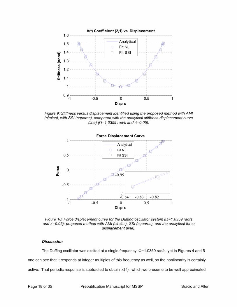
be integrated with respect to the measured displacement for each instant in the periodic orbit in order to

obtain the force-displacement curve for the system. The resulting force-displacement curve is plotted in

Figure 10, revealing that the force-displacement relationship is cubic. If desired, one could fit a cubic

polynomial to this curve to estimate k and k3, or this curve could be used directly to simulate the response

of the nonlinear system. The inset plot shows a detailed view of the force-displacement curve at the

extreme end of its range. In both Figures 9 and 10, the open blue circles are the values obtained by AMI,

the open black squares are the values calculated from the identified SSI model, and the blue lines are the

analytical results. The values found using the frequency-domain AMI algorithm agree well with those

obtained by the time-domain SSI algorithm and both agree well with the analytical results, so for these

simulated measurements either could be used.


-1 -0.5 0 0.5 10.9

1

1.1

1.2

1.3

1.4

1.5

1.6

Disp x

Sti

ffn

ess

(no

nd

)

A(t) Coefficient (2,1) vs. Displacement

Analytical

Fit NL

Fit SSI

Figure 9: Stiffness versus displacement identified using the proposed method with AMI (circles), with SSI (squares), compared with the analytical stiffness-displacement curve

(line) (=1.0359 rad/s and A=0.05).

-1 -0.5 0 0.5 1-1

-0.5

0

0.5

1

Disp x

Fo

rce

Force Displacement Curve

Analytical

Fit NL

Fit SSI

-0.84 -0.83 -0.82-1

-0.95

Figure 10: Force displacement curve for the Duffing oscillator system (=1.0359 rad/s and A=0.05): proposed method with AMI (circles), SSI (squares), and the analytical force

displacement (line).

Discussion

The Duffing oscillator was excited at a single frequency, =1.0359 rad/s, yet in Figures 4 and 5

one can see that it responds at integer multiples of this frequency as well, so the nonlinearity is certainly

active. That periodic response is subtracted to obtain ( )x t , which we presume to be well approximated


as linear time periodic. The response of the system before lifting, shown in Figure 5 contains several

peaks. The largest peak is at 1.1 rad/s, so it can be attributed to the time periodic mode and one would

take 1 1.1rad/s . If the system were linear then its linearization about the limit cycle would not

depend on time and only this peak would occur. However, this system is nonlinear and hence its

linearization is time periodic giving rise to several other peaks in the response corresponding to

1 Tim as explained by Eq. (7). The peak at 0.98 rad/s just to the left of the zero harmonic is the

negative second harmonic term which would appear at 1.1 rad/s – 2*1.04 rad/s = -0.98 rad/s, but it folds

back to +0.98 rad/s. The peak at 3.18 rad/s is the positive second harmonic of the mode at 1.1 rad/s +

2*1.04 rad/s = 3.18 rad/s, and so on. One should also note that if the system was purely linear, one

would expect the zero harmonic frequency content to occur at the linear natural frequency of 1 rad/s

instead of at 1.1 rad/s, but for a time periodic system the response peaks at the Floquet exponent, which

is usually not equal to the natural frequency of the linearized system. All of this information could be used

to construct a time periodic model for this system’s mode using the information in Figure 5, but as was

mentioned in Section 2, it is much more convenient to first lift the measurements.

The spectra that result after applying the lifting technique are much simpler to interpret and show

only one peak for this single-degree-of-freedom system. The composite spectrum contains only one

strong peak and AMI fits a single mode to the peak with a natural frequency of 1 0.0624 rad/s . This is

an alias of the dominant frequency at 1.1 rad/s in Figure 5, as expected because the lifting technique

resamples the measurement once per period, changing the effective bandwidth of the signals. The

aliasing is of little consequence because the aliased Floquet exponent provides a perfectly valid

description of the linear time periodic system. The model identified by AMI was then used to reconstruct

the state matrix and eventually the force-displacement relationship of this nonlinear system. It is

significant to note that the entire identification was performed without having to assume the functional

form of the restoring force a priori. The only assumption was that the periodic orbit was stable and that

the response could be approximated as linear time periodic about that orbit.


3.2. Effect of other Excitation Configurations

Using this method, one is able to identify a nonlinear model for a system about its entire periodic

orbit, whereas a traditional approach would identify a linearized model that is valid near a single

configuration of the system. The periodic orbits and response of a nonlinear system depend strongly on

several factors including the drive force amplitude and frequency and impulse force amplitude and

duration, and it is therefore necessary to consider how different forcing configurations affect the nonlinear

identification proposed here. This was explored by computing the nonlinear frequency response of the

Duffing oscillator for a few harmonic forcing amplitudes using the methods in [23]. The result for

harmonic forcing amplitude A=0.1 is shown in Figure 11 where each point on the curve represents a

stable (solid curves) or unstable (dashed curve) periodic orbit. The figure clearly shows a superharmonic

resonance peak and the spring hardening region (shaded region), which is also the region where multiple

periodic orbits are possible for a single forcing frequency. In the previous section, it was shown that the

identification could be applied successfully when the system was excited in a region just below resonance

(with harmonic forcing amplitude A=0.05), and the corresponding region for A=0.1 is labeled below. In

Sections 3.2.1-3.2.3, the identification will be explored for two orbits in the region where multiple solutions

are possible, MS Orbit 1 and MS Orbit 2 in Figure 11, for a Superharmonic orbit that would be located on

a Superharmonic resonance similar to that labeled in the figure, and for excitations that exhibit period

lengthening effects (such as period doubling, [12] pages 70-91).


0 0.5 1 1.5 210

-4

10-2

100

Am

pli

tud

e D

isp

lace

men

t

Frequency, rad/s

Nonlinear Frequency response

Figure 11: Spring hardening nonlinear frequency response with superharmonic resonance for harmonic forcing amplitude A=0.1.

3.2.1. Excitation Producing Multiple Well-Separated Orbits

As mentioned previously, this system has different types of periodic solutions depending on the

forcing frequency. In the shaded region of Figure 11, there are three possible responses for a single

forcing frequency, one of which is unstable. Although it cannot be realized in experiment, an unstable

periodic orbit can be simulated. This configuration would certainly not be suitable for identification by this

method, because the response of the system would not return to the unstable periodic orbit after being

perturbed, but would jump to a nearby stable periodic orbit. When multiple stable periodic orbits are

possible for a single forcing, the identification can theoretically be performed using any of the periodic

orbits, presuming that the perturbations are small enough to keep the response of the system close to the

originating orbit.

This was explored using a drive frequency and amplitude of Ω = 1.3566 rad/s and A = 0.1, which

is a configuration that has stable periodic orbits that can be initiated from T,x x = [-0.0039, -0.1622]T

(Multiple Solutions orbit 1) and T,x x = [-1.2019, 2.402]T (Multiple Solutions Orbit 2). Figure 12 shows

the state space portraits of the two stable periodic orbits for this forcing configuration. The response in

Multiple Solution Orbit 2, shown with the dashed black curve (MS Orbit 2), has much greater amplitude

than that of Multiple Solution Orbit 1 shown in blue (MS Orbit 1).

MS Orbit 1

MS Orbit 2 Superharmonic Resonance

Excitation Near Resonance

Spring Hardening


-3 -2 -1 0 1 2 3-3

-2

-1

0

1

2

3

Displacement

Vel

oci

ty

Phase Space Portraits of the Periodic Orbits

MS Orbit 1

MS Orbit 2

Figure 12: State space portraits of two stable periodic orbits that exist for a forcing frequency Ω = 1.3566 rad/s at forcing amplitude A=0.1.

Following the exact same procedure as in Section 3.1, the state coefficient matrices were

identified for both these periodic orbits. The stiffness terms are shown in Figure 13 with the values for the

MS Orbit 1 plotted with filled blue squares, the values for MS Orbit 2 plotted with open blue circles, and

the values from the analytical model plotted with blue lines. The force displacement relationship was

constructed for each identified model and those curves are shown in Figure 14. The inset plot shows a

detailed view of the curves near the origin. The identified system for the MS Orbit 2 is significantly time

periodic, since the stiffness varies over the period by 450% of the initial stiffness value, while the system

for MS Orbit 1 is approximately linear time invariant. As a result, the force-displacement curve for MS

Orbit 2 is very nonlinear, while the force displacement curve for MS Orbit 1 is very linear and only

captures the force-displacement relationship over a small range. Both of the identified models compare

very well to their corresponding analytical state coefficient models, verifying that the proposed

identification method works even when the input produces multiple periodic orbits that are stable and well

separated.


0 1 2 3 4 5-5

-4

-3

-2

-1

0


time (s)

Co

effi

cien

t

A(2,1) Analytical

A(2,1) MS Orbit 1

A(2,1) MS Orbit 2

Figure 13: Components of the state coefficient matrix that correspond to the instantaneous stiffness of the system for an entire periodic orbit for MS Orbit 1 and 2

(=1.3566 rad/s and A=0.1).

-3 -2 -1 0 1 2 3

-6

-4

-2

0

2

4

6


Disp x

Fo

rce

-0.1 -0.05 0 0.05 0.1-0.2

0

0.2

Analytical

MS Orbit 1MS Orbit 2

Figure 14: Force displacement curves for the MS Orbits 1 and 2 (=1.3566 rad/s and A=0.1).

3.2.2. Superharmonic Resonance

Nonlinear systems such as this may also exhibit superharmonic resonance, where an excitation

at some fraction of the linear natural frequency excites a resonant response. This type of orbit could also


be used to perform the proposed system identification. This was explored for the Duffing oscillator using

an amplitude of A=1 and a driving frequency of Ω=0.3934 rad/s, which corresponds to a Superharmonic

orbit where the drive frequency is near one third of the linear natural frequency [22] of 1 rad/s. The initial

conditions Tx x = [-0.5695, 1.1170]T were used as the starting point when computing both the periodic

and perturbed responses. The same impulsive forcing conditions were used. The solutions were

evaluated with a sampling frequency of approximately fsamp= 2.76 Hz, which results in 44 samples per

cycle of the harmonic response. Both responses were evaluated for a time window length containing 614

full cycles of the harmonic response frequency. Figure 15 shows the time responses of the

Superharmonic orbit in the same format as Figure 3. The time histories show that the resulting periodic

and perturbed responses contain at least two prominent frequencies.

0 5 10 15 20 25-2

-1

0

1

2

time, s

Dis

p

Early Time Response

750 755 760 765 770 775-2

-1

0

1

2

time, s

Late Time Response

xPerturbed

xPeriodic

0 100 200 300 400 500 600 700 800 900-0.2

-0.1

0

0.1

0.2

time, s

Dis

p

Approximate LTP Response

xLTP Approx

Figure 15: Response of the nonlinear Duffing oscillator excited by harmonic (=0.3934 rad/s and A=1) excitation near a superharmonic resonance and impulsive excitation. Plots (a) and (b) provide the early and late time history, respectively, of the periodic

response (dashed red) and the perturbed response (solid black). Plot (c) is the resulting linear time periodic response obtained by subtracting the two signals in (a) and (b).

The lifting technique was applied and the 44 lifted responses were processed with AMI. AMI


identified an eigenvalue of 1=-0.0079 + 0.0343i, a natural frequency of |1|=0.0352 rad/s, and a damping

ratio of Re(-1)/|1| =0.2243 for the linear time periodic system. The Fourier series expansion method

was then applied to the extracted mode. Figure 16 shows amplitudes of each of the coefficients in the

Fourier series expansion of the mode. The open blue circles are all of the coefficients that were identified

from the lifted response and the red dots are the coefficients of expansion terms that were retained when

computing A(t).

-30 -20 -10 0 10 20 3010

-6

10-4

10-2

Fourier Series Coeff (m)

Am

pli

tud

e

Fourier Series Expansion of LTP Mode

All

kept

Figure 16: Fourier Series expansion of the linear time periodic model from the Superharmonic orbit (=0.3934 rad/s and A=1). (open blue circles) Fourier coefficients

of the identified mode. (solid red circles) Dominant Fourier coefficients that were kept for the model.

Figure 16 shows that at least 10 terms are dominant in the Fourier expansion of the mode shape.

The state transition and state coefficient matrix were constructed using these 10 terms. Figure 17 shows

the stiffness and damping terms in the state coefficient matrix that were identified by the proposed

method. The Stochastic Subspace system identification and the analytical results are also shown. The

identified damping term is nearly constant with some small variations about the nominal damping value.

The stiffness of the system is highly time periodic, varying by up to 250% of its initial value. It also varies

in a more complicated way than it did in Figure 8, since the periodic orbit is more complicated. Both the

stiffness and damping coefficients identified with the proposed frequency domain technique and the SSI

method compare very well to the analytical results.


0 2 4 6 8 10 12 14 16-3

-2.5

-2

-1.5

-1

-0.5

0

0.5

time (s)

Co

effi

cien

t


A(2,1) AnalyticalA(2,1) Fit NL

A(2,1) Fit SSI

A(2,2) Analytical

A(2,2) Fit NLA(2,2) Fit SSI

Figure 17: Components of the state coefficient matrix that correspond to the instantaneous stiffness (component (2,1)) and damping (component (2,2)) of the system

for the Superharmonic orbit (=0.3934 rad/s and A=1).

Figure 18 shows the identified instantaneous stiffness coefficient plotted versus the displacement

of the system and Figure 19 shows the force-displacement curve reconstructed from this result. The

analytical and SSI results are shown for comparison. These results show that although the stiffness of

the system varies with time in a much more complicated way, the stiffness versus displacement

relationship still follows a quadratic relationship and the restoring force is cubic as before. It is noteworthy

that such a drastically different periodic orbit could give a result that is so similar to that obtained from the

much simpler orbits that were studied in Sections 3.1 and 3.2.1.


-1.5 -1 -0.5 0 0.5 1 1.50.5

1

1.5

2

2.5

3

Disp x

Sti

ffn

ess

(no

nd

)

A(t) Coefficient (2,1) vs. Displacement

Analytical

Fit NL

Fit SSI

Figure 18: Displacement varying terms from the estimated (circles) and analytical A(t) (line) matrix plotted versus the displacement for the Superharmonic orbit (=0.3934 rad/s

and A=1).

-1.5 -1 -0.5 0 0.5 1 1.5-3

-2

-1

0

1

2

3

Disp x

Fo

rce

f


Analytical

Fit NL

Fit SSI

-1.48 -1.46 -1.44

-2.25

-2.2

-2.15

Figure 19: Force-displacement curve for the A(t) matrix plotted versus the displacement for the Superharmonic orbit (=0.3934 rad/s and A=1).

3.2.3. Effect of Period Lengthening

Several texts on nonlinear systems theory mention the fact that a system with a stable periodic

orbit can sometimes respond with a period that is longer than that of the input. Typically, as some

parameter such as the forcing amplitude is increased, one observes that the fundamental frequency of


the response, which is initially Ω, first becomes Ω/2, then Ω/3, etc… so that the fundamental period of the

orbit doubles, then triples, etc… [12, 25]. This would certainly affect the proposed system identification

strategy, so it deserves consideration, even if this type of behavior is difficult to predict analytically.

0 1 2 3 4 5 6

10-6

10-4

10-2

100

Frequency, rad/s

Mag

- F

FT

Dis

p

FFT of Response

Figure 20: FFT spectrum of perturbed nonlinear response of the period tripled limit cycle of the Multiple Solutions Orbit 2.

The authors have observed period lengthening when simulating identification of the Duffing

system. For example, this was observed in Multiple Solutions Orbit 2 from Section 3.2.1. Figure 20

shows the frequency spectrum of the simulated periodic plus perturbation response for that case. As

was noted for the spectrum shown in Figure 4, the response spectrum has sharp peaks at the input

frequency, Ω=1.356 rad/s and its third harmonic, 3Ω=4.068rad/s, and also shows the presence of the

linear time periodic mode at 1.27, 1.44, 3.98, and 4.15 rad/s. However, this spectrum also shows several

other peaks. The lowest appears at 0.452 rad/s and all of the others are integer multiples of this

frequency: 2.260, 3.164, and 4.972 rad/s. Relative to the drive frequency, 0.452 rad/s is Ω/3 and the

other frequencies are (5/3)Ω, (7/3)Ω and (11/3)Ω. This spectral content could only be present if the

response of the system has a period that is three times as long as the period of the forcing, revealing that

this is a case of period-tripling. One could account for this in the proposed identification scheme by

simply noting that the period of ( )x t is actually three times longer than the period of the input. All other

1.356 4.068

1.44

0.452

4.15 1.27

2.260

3.164

3.98

4.972


steps in the proposed identification algorithm could remain the same. However, it is also possible the

new length 3T periodic orbit remains very close to the original length T orbit even though the period has

lengthened and if this is the case then one might be able to ignore the fact that the period has

lengthened.

To investigate this, the phase portrait of the orbit is plotted in Figure 21 over many cycles of the

response. Surprisingly, this appears to be the same as the original length T limit cycle. Closer inspection

reveals that there are actually three curves, as illustrated by the two inlaid plots. These curves could be

traced around the phase plane, revealing that one must complete three loops before the response

repeats itself. However, these curves always remain very close to the original length T orbit. Since the

state of the system is practically the same at each point along the length T and length 3T orbits, one can

ignore the period lengthening in this case and process the measurement as described in the previous

section. However, if one takes this approach, then the Ω/3 (or, in general, Ω/N) harmonics in the

spectrum would not be removed when subtracting ( )x t from the measurements. They should be ignored

when performing system identification since they are a property of the orbit and not of the time periodic

approximation about that orbit. If this is done, good results can still be achieved as was shown in Section

3.2.1.

-3 -2 -1 0 1 2 3-3

-2

-1

0

1

2

3

Displacement

Vel

oci

ty

Phase Space Portrait of Periodic Orbit

-1.655-1.65-1.645-1.975-1.97

-1.965

1.271.2751.282.355

2.36

2.365

Figure 21: State space portrait of the period tripled limit cycle of the Multiple Solutions Orbit 2 after the perturbation was applied.


3.3. Effect of Excitation and Perturbation Amplitudes

As explained in Section 2, the time periodic model that this method is based upon is only valid if

the system remains near the periodic orbit. However, the periodic orbit dictates the range of the

measurement sensors, so one would like make the perturbation as large as possible to assure that it is

not buried in measurement noise. Furthermore, the previous sections have shown that the excitation

affects the complexity of the time periodic model, dictating the number of harmonics that must be

extracted from a measurement to adequately characterize the system. This section explores these issues

for the Duffing system by varying the periodic orbit and the perturbation from that orbit and evaluating the

effect on the identified time periodic model.

The strength of the perturbation from the periodic orbit is quantified by computing the ratio of the

amplitudes of the response and the perturbation in the frequency domain, which is denoted

max ( )100

max ( )

X

X

(15)

where the capital letters X and X denote that these are the Fourier transforms of ( )x t and ( )x t

respectively and multiplication by 100 makes a percentage. This is illustrated in Figure 5.

The complexity of the time periodic system model can be characterized by the Fourier coefficients

of the time-periodic mode shape (e.g. those shown in Figures 7 and 16). The relative amplitudes give a

measure of the complexity so these are denoted Bn for any integer n. The simplest possible model for the

system about the limit cycle is a time invariant one, where B0 =1 and Bn =0 for all other n. The coefficients

for n0 generally become larger as the complexity of the time periodic system model increases, as was

illustrated in Sections 3.1 and 3.2.2.

These metrics were calculated for forcing amplitudes A=0.01 and 0.1 in Eq. (13), forcing

frequencies Ω=0.3802 and 0.9868 rad/s, and perturbation magnitudes that gave =0.5% and 2%. Table

1 provides the results. The two driving frequencies considered are near one third the linear natural

frequency and just below the linear natural frequency, similar to those that were found to produce good

results in Sections 3.1 and 3.2.2. The top block labeled (a) gives the results for driving force amplitude


A=0.01 while the bottom block corresponds to A=0.1. The relative amplitudes of the Fourier coefficients

B-2, B0 and B2 are shown for each case. These were obtained by applying a curve fit to the lifted spectrum

as described in the previous sections and then finding the ratio of the Fourier coefficient amplitudes. The

analytical Fourier coefficients were also calculated for each case and are shown.

(a) A=0.01

Ω = 0.3802 rad/s Ω = 0.9868 rad/s

(%) Analytical 0.5% 2.0% Analytical 0.5% 2.0%

B-2 0.0000 0.0001 0.0000 0.1141 0.1124 0.1018

B0 1 1 1 1 1 1

B2 0.0000 0.0002 0.0001 0.0014 0.0020 0.0035

(b) A=0.1

Ω = 0.3849 rad/s Ω = 0.9821 rad/s

(%) Analytical 0.5% 2.0% Analytical 0.5% 2.0%

B-2 0.0027 0.0027 0.0030 0.2337 0.2316 0.1905

B0 1 1 1 1 1 1

B2 0.0012 0.0010 0.0019 0.0123 0.0123 0.0080 Table 1: Fourier coefficients of the identified linear time periodic mode for various drive

amplitudes, A, frequencies, Ω, and perturbation amplitudes, . The results show that the Fourier coefficients begin to differ from the true, analytical values if the perturbation

amplitude is too large.

When A=0.01 and Ω=0.3802 rad/s the response is almost purely linear and the only significant

Fourier term is the linear term (B0). The Fourier coefficients for both low (=0.5%) and larger (=2%)

deviation from the periodic orbit are less than 0.0002, so the identification procedure would apparently be

accurate under these conditions, although not all that useful since the nonlinearity is not well excited.

When the excitation frequency is increased to Ω=0.9868 rad/s, the B-2 harmonic is approximately 11% as

strong as the dominant term indicating that the nonlinearity is active. When the perturbation amplitude is

=0.5%, the B-2 and B2 coefficients are identified within 0.002 and 0.0006 of the analytical values,

respectively. However, when the perturbation is increased to =2%, the identified Fourier coefficients

differ from the true values by more than 0.01 and 0.002 respectively. Even at this level of , the

reconstructed force-displacement curves were still reasonable which shows that the method is quite

robust to errors in the identified Fourier coefficients.

Increasing the magnitude of the driving force to A=0.1 increases the coefficients B-2 and B2 for all

of the cases, indicating that the nonlinearity is more active and so the time-periodic approximation is more

complicated. In all of these cases, when the perturbation amplitude is small, =0.5%, the Fourier


coefficients are accurate to within 0.0021 for B-2 and 0.0002 for B2. When the perturbation amplitude was

increased to =2%, the errors in the coefficients increase to 0.04 and 0.004 respectively. For this system

it seems that the perturbation amplitude must be about 0.5% or less in order to accurately identify a time

periodic model for the system. Hence, fairly accurate sensors will be needed to apply this method in

practice.

4. Conclusions

This work presented a new experimental system identification method that is based on linearizing

a nonlinear system about a periodic orbit, measuring the perturbation of the system from that orbit and

identifying a linear time periodic model for the perturbed dynamics. The main advantage of the method is

that it characterizes the system’s nonlinearity non-parametrically, so there is no need to assume the

functional form of the nonlinearity a priori. Also, linear system identification techniques can be used to

identify the time-periodic model, greatly simplifying the interpretation of the measurements and

identification of the system parameters.

The method was evaluated by applying it to simulated measurements of a single degree-of-

freedom system with a cubic nonlinearity. The following observations were made.

Identification was successful under a broad range of excitation frequencies and amplitudes, so

long as the amplitude of the periodic orbit was large enough to exercise the nonlinearity.

Some periodic orbits are more complicated than others, for example when the system is excited

at a superharmonic resonance. This makes the underlying linear time periodic model more

complicated as well, perhaps increasing the chance that an important harmonic might be missed,

but the cases studied here still seemed to produce good results.

One forcing configuration was observed, in a region where multiple responses were possible for a

single forcing frequency, where the system’s response had a larger period than the input. Even

in this case, the system was accurately identified because the lengthened orbit remained close to

the original orbit.

The linear time periodic approximation is only accurate if the system’s response remains very

close to the periodic orbit. For the system studied here, adequate results were obtained if the


amplitude of the perturbation was less than 0.5% of the periodic orbit amplitude. Hence, fairly

accurate sensors will be needed to implement the method experimentally.

The identification extends very naturally to higher order systems. As demonstrated here, the

measurements are easy to interpret in the frequency domain, and as with familiar time invariant systems,

additional degrees of freedom simply manifest themselves as additional peaks in the spectra. The

system identification routines used to extract the time periodic modes can readily accommodate

measurements with relatively large numbers of modes. On the other hand, higher order systems can

exhibit even more complicated periodic orbits, so one will have even more freedom in selecting the

optimal periodic forcing function. These issues will be explored in future works.

5. Acknowledgements

This material is based on work supported by the National Science Foundation under Grant No.

CMMI-0969224 and in part by Sandia National Laboratories. Sandia is a multiprogram laboratory

operated by Sandia Corporation, a Lockheed Martin Company, for the United States Department of

Energy’s National Nuclear Security Administration under Contract DE-AC04-94AL85000.

References [1] G. Dimitriadis and J. Li, "Bifurcation of Airfoil Undergoing Stall Flutter Oscillations in Low-Speed

Wind Tunnel," AIAA Journal, vol. 47, pp. 2577-2596, 2009.

[2] G. Kerschen, et al., "Past, Present and Future of Nonlinear System Identification in Structural Dynamics," Mechanical Systems and Signal Processing, vol. 20, pp. 505-592, 2006.

[3] G. L. Gray, et al., "Chaos in a Spacecraft Attitude Maneuver Due to Time-Periodic Perturbations," Journal of Applied Mechanics, vol. 63, pp. 501-508, 1996.

[4] I. Dobson, et al. (1992) Voltage Collapse in Power Systems, Circuit and System Techniques for Analyzing Voltage Collapse are Moving Toward Practical Application - and None too Soon. IEEE Circuits and Devices Magazine. 40-45.

[5] S. L. Lacy and D. S. Bernstein, "Subspace Identification for Non-Linear Systems With Measured-Input Non-Linearities," International Journal of Control, vol. 78, pp. 906-926, 2005.

[6] D. E. Adams and R. J. Allemang, "Survey of Nonlinear Detection and Identification Techniques for Experimental Vibrations," in Proceedings of the International Conference on Noise and Vibration Engineering, 1998, pp. 269-281.

[7] K. Worden and G. R. Tomlinson, "A Review of Nonlinear Dynamics Applications to Structural Health Monitoring," Strucrural Control and Health Monitoring, vol. 15, pp. 540-567, 2007.


[8] P. Hartman, "Linearizations, Periodic Solution, Limit Cycles, Smooth Linearizations," in Ordinary Differential Equations, ed New York: John Wiley & Sons, Inc., 1964, pp. 244-259.

[9] M. S. Allen, "Frequency-Domain Identification of Linear Time-Periodic Systems Using LTI Techniques," Journal of Computational and Nonlinear Dynamics, vol. 4, pp. 041004.1-6, 2009.

[10] M. S. Allen and J. H. Ginsberg, "A Global, Single-Input-Multi-Output (SIMO) Implementation of The Algorithm of Mode Isolation and Applications to Analytical and Experimental Data," Mechanical Systems and Signal Processing, vol. 20, pp. 1090–1111, 2006.

[11] P. Van Overschee and B. De Moor, Subspace Identification for Linear Systems: Theory-Implementation-Applications. Boston: Kluwer Academic Publishers, 1996.

[12] J. Guckenheimer and P. Holmes, Nonlinear Oscillations, Dynamical Systems, and Bifurcations of Vector Fields vol. 42. New York: Springer-Verlag New York Inc., 1983.

[13] J. W. Larsen and S. R. K. Nielsen, "Nonlinear Parametric Instability of Wind Turbine Wings," Journal of Sound and Vibration, vol. 299, pp. 64-82, 2007.

[14] C. Basdogan and F. M. L. Amirouche, "Nonlinear Dynamics of Human Locomotion: From the Perspective of Dynamical Systems Theory.," in Engineering Systems Design and Analysis Conference, 1996.

[15] J. B. Dingwell and J. P. Cusumano, "Nonlinear time series analysis of normal and pathological human walking," Chaos, vol. 10, pp. 848-63, 2000.

[16] J. B. Dingwell and K. Hyun Gu, "Differences between local and orbital dynamic stability during human walking," Transactions of the ASME. Journal of Biomechanical Engineering, vol. 129, pp. 586-93, 2007.

[17] G. Floquet, "Sur Les Equations Lineairs a Coefficients Periodiques," Ann. Sci. Ecole Norm. Sup., vol. 12, pp. 47-88, 1883.

[18] P. Friedmann and C. E. Hammond, "Efficient Numerical Treatment of Periodic Systems with Application to Stability Problems," International Journal for Numerical Methods in Engineering, vol. 11, pp. 1117-1136, 1977.

[19] L. Meirovitch, Methods of Analytical Dynamics. New York: McGraw-Hill Book Company, 1970.

[20] M. S. Allen and M. W. Sracic, "System Identification of Dynamic Systems with Cubic Nonlinearities Using Linear Time-Periodic Approximations," presented at the ASME 2009 International Design Engineering Technical Conference IDETC, San Diego, California, USA, 2009.

[21] M. S. Allen and J. H. Ginsberg, "Floquet Modal Analysis to Detect Cracks in a Rotating Shaft on Anisotropic Supports," in 24th International Modal Analysis Conference (IMAC XXIV), St. Louis, MO, 2006.

[22] A. H. Nayfeh and D. T. Mook, Nonlinear Oscillations. New York: John Wiley and Sons, 1979.

[23] M. W. Sracic and M. S. Allen, "Numerical Continuation of Periodic Orbits for Harmonically Forced Nonlinear Systems," presented at the 29th International Modal Analysis Conference (IMAC XXIX), Jacksonville, Florida, USA, 2011.

[24] M. W. Hirsch and S. Smale, Differential Equations, Dynamical Systems, and Linear Algebra. New


York: Academic Press, Inc, 1974.

[25] R. U. Seydel, Practical Bifurcation and Stability Analysis: From Equilibrium to Chaos, 2nd ed. New York: Springer-Verlag, 1994.

Method for Identifying Models of Nonlinear Systems Using ...

Documents

Transcript of Method for Identifying Models of Nonlinear Systems Using ...