.

NASA Technical Memorandum 100935

Method and Models for R-Curve Instability Calculations

Thomas W. Orange Lewis Research Center Cleveland, Ohio

Prepared for the Twenty-first National Symposium on Fracture Mechanics sponsored by the American Society for Testing and Materials Annapolis, Maryland, June 28-30, 1988

https://ntrs.nasa.gov/search.jsp?R=19880013894 2018-10-09T23:43:57+00:00Z

METHOD AND MODELS FOR R-CURVE INSTABILITY CALCULATIONS

Thomas W . Orange National Aeronautics and Space Administration

Lewis Research Center Cleveland, Ohio 44135

SUMMARY

This paper presents a simple method for performing elastic R-curve insta- bility calculations. For a single material-structure combination, the calcula- tions can be done on some pocket calculators. On microcomputers and larger, it enables the development of a comprehensive program having libraries of driv- ing force equations for different configurations and R-curve model equations for different materials. The paper also presents several model equations for fitting to experimental R-curve data, both linear elastic and elastoplastic. The models are fit to data from the literature to demonstrate their viability.

INTRODUCTION

The R-curve is one of the most powerful concepts available to the fracture analyst. It is probably the best phenomenological description of the mono- tonic fracture process currently available. But it has not received the acclaim and widespread use that it deserves. Perhaps the instability calcula- tions are thought to be too involved o r tedious. The literature contains very little information on instability calculations and nothing recent. Creager (ref. 1 ) presented a good graphical method. But it involves overlay transpar- encies, is labor-intensive, and may lack precision. In a predictive round- robin program (ref. 2 1 , seven participants used the R-curve method. Only this author used anything more elaborate than trial-and-error t o perform the insta- bi l i ty calculations.

The method I used Is really quite simple. For a single material-structure combination, the calculation can be done on some pocket calculators. On micro- computers and larger, a comprehensive program having libraries o f driving force equations and R-curve model equations is possible.

This paper will describe the method of performing the instability calcula- tion. It will also present several model equations for fitting to experimen- tal R-curve data, both linear-elastic (K,G) and elastoplastic ( 3 ) .

SYMBOLS

a crack length

A,B ,C,D,F,H empirical coefficients in equations (3) t o ( 7 )

G strain energy release rate

J nonlinear crack parameter

K stress intensity factor

L,M,N,P e m p i r i c a l c o e f f i c i e n t s i n equa t ions (8) t o (11)

W w i d t h o f specimen (or s t r u c t u r e )

Y s t r e s s i n t e n s i t y c a l i b r a t i o n f a c t o r

A c r a c k e x t e n s i o n ( e f f e c t i v e or p h y s i c a l , as no ted)

f low S t r e s s O f

Subsc r ip t s :

0 a t i n i t i a l (un loaded) c o n d i t i o n

C c r i t i c a l , a t t h e i n s t a b i l i t y p o i n t

R r e l a t e d t o t h e m a t e r i a l ' s r e s i s t a n c e

Specimen N o t a t i o n :

M(T) cen te r -c rack t e n s i o n

cs r e c t a n g u l a r compact

CLWL c r a c k - l i n e wedge loaded

INSTABILITY CALCULATION METHOD

The method was p resen ted p r e v i o u s l y ( r e f . 3 > , b u t w i l l be repea ted here . The i n s t a b i l i t y c o n d i t i o n r e q u i r e s t h a t b o t h t h e magni tudes and t h e s lopes o f the c rack d r i v i n g f o r c e ( G or K ) curve and t h e m a t e r i a l r e s i s t a n c e cu rve (GR) be equal a t t h e p o i n t o f i n s t a b i l i t y . So we must s o l v e two s imu l taneous equa- t i o n s . A f t e r w r i t i n g t h e equa t ions i n a genera l form and d o i n g a l i t t l e a lge - b r a , we can w r i t e the i n s t a b i l i t y c o n d i t i o n as

where

and a = (a /Y) (dY/da)

For e l a s t i c R-curves A i s t h e e f f e c t i v e c r a c k ex tens ion , a. i s t h e i n i - t i a l c rack l e n g t h , Y i s t h e s t r e s s i n t e n s i t y c a l i b r a t i o n f a c t o r , and t h e sub- s c r i p t ( c ) means "eva lua ted a t t h e i n s t a b i l i t y p o i n t . " ( I f you p r e f e r t o work w i t h the s t r e s s i n t e n s i t y f a c t o r K, s u b s t i t u t e K / Z K ' for G I G ' . ) Now i f we p u t i n the express ions f o r GR, G i , and a then, for p r e s c r i b e d va lues o f a, and specimen w i d t h W , A, i s t h e l e a s t p o s i t i v e root o f e q u a t i o n ( 1 ) . Any o f severa l numer ica l methods w i l l s o l v e for t h e root, even on a programmable hand c a l c u l a t o r . Once Ac i s known, we can c a l c u l a t e Gc and t h e f a i l u r e s t r e s s . The beauty o f t h i s e q u a t i o n i s t h a t t h e f irst t e r m on t h e r i g h t s i d e i s a f u n c t i o n o f t h e m a t e r i a l ' s R-curve o n l y and t h e second i s a f u n c t i o n o f t h e

2

s t r u c t u r a l geometry o n l y . Equat ions f o r t h e second t e r m can be o b t a i n e d from s tandard handbooks and w i l l n o t be d iscussed here . Model R-curve equa t ions to be used i n t h e f i r s t t e r m w i l l be d iscussed l a t e r .

The e f f e c t i v e n e s s of t h i s method i s shown i n appendix 1 1 o f ( r e f . 2). I n t h a t a n a l y t i c a l round- rob in program, good p r e d i c t i o n s o f f r a c t u r e s t r e n g t h s were made f o r bo th s imp le and complex specimen geometr ies.

U n f o r t u n a t e l y t h i s s imp le method i s n o t a p p l i c a b l e t o e l a s t i c - p l a s t i c ( J R ) c a l c u l a t i o n s . As d iscussed i n Sec t i ons ( 2 and 6) o f ( r e f . 4 ) , t h e problem i s much more compl ica ted . M a t e r i a l p r o p e r t i e s a re an i n t e g r a l p a r t o f t h e ca l cu - l a t i o n o f t h e d r i v i n g fo rce ( J ) , and t h e r e appears to be no genera l way t o sep- a r a t e them from t h e geomet r i ca l t e r m s . However, t he model equa t ions f o r JR curves t o be d iscussed l a t e r may s t i l l p rove u s e f u l .

ELASTIC R-CURVE MODELS

To do these c a l c u l a t i o n s we need an equa t ion f o r the R-curve. Whi le i t would be n i c e i f t h e e q u a t i o n had some p h y s i c a l s i g n i f i c a n c e , i t ' s n o t abso- l u t e l y necessary. U n t i l a good t h e o r e t i c a l a n a l y s i s i s a v a i l a b l e , a l l we need i s a cont inuous e q u a t i o n t h a t approx imates r e a l i t y , i s r e a d i l y d i f f e r e n t i a b l e , and f i t s t h e da ta . R-curve da ta . But t h e r e a re seve ra l usab le equat ions , so we have to p i c k the one t h a t b e s t f i t s t h e p a r t i c u l a r da ta . L e t 'R ' be a g e n e r i c te rm t o i n d i - c a t e e i t h e r GR or KR.

A t p resen t t h e r e i s no s i n g l e equa t ion t h a t f i t s a l l

Wang and McCabe ( r e f . 5) suggested f i t t i n g a po lynomia l t o d a t a i n t h e r e g i o n o f t h e R-curve where you expec t i n s t a b i l i t y to occur . d e s c r i b e t h e e n t i r e curve by a low-order (say, c u b i c ) s p l i n e f u n c t i o n . For e i t h e r case we have

One c o u l d a l s o

RO = A0 + A1A + A2A2 + A3A3 ( 2 )

( n o t e : d i f f e r e n t po l ynomia l c o e f f i c i e n t s a r e used for each s p l i n e segment.)

Broek and V l i e g e r ( r e f . 6) suggested a power curve o f t h e form

~1 = AAB (3 )

where O<B<1. Th i s p a r t i c u l a r form works v e r y w e l l for the more d u c t i l e m a t e r i - a l s such as 2000-ser ies aluminums and some s t a i n l e s s s t e e l s . I t has two unique f e a t u r e s . The s lope i s i n f i n i t e a t A = 0, and t h e r e i s no asymptote. I n p h y s i c a l terms these i m p l y t h e r e i s no c r a c k e x t e n s i o n a t smal l l oads (wh ich i s t e n a b l e ) and t h a t a m a t e r i a l ' s f r a c t u r e toughness i s l i m i t e d o n l y by t h e s i z e o f t h e specimen (wh ich i s n o t ) . So i t may n o t be a good fundamental model, b u t i t ' s q u i t e good f o r curve f i t t i n g .

Lower-toughness m a t e r i a l s a r e u s u a l l y asympto t i c t o a p l a t e a u v a l u e ' o f toughness. Severa l models f i t t h i s d e s c r i p t i o n . Bluhm ( r e f . 7) proposed an e x p o n e n t i a l model,

T h i s form has a f i n i t e s lope a t A = 0 and i s asympto t ic to R;. A somewhat s i m i l a r model, which I w i l l c a l l t h e h y p e r b o l i c model, i s

3

Th is i s a c t u a l l y an i n v e r t e d and t ransposed r e c t a n g u l a r hyperbo la . L i k e t h e

exponen t ia l model i t has a f i n i t e s lope a t A = 0 and i s asympto t ic t o R3.

Tr igonometry suggests two a d d i t i o n a l asympto t ic forms. They a re the arc ta r i - gent f u n c t i o n

lk

R4 = Ri(2/7r) arc tan(wA/2F) (6)

and the h y p e r b o l i c tangent R 5 = RE tanh(A/H) ( 7 )

The power model, equa t ion ( 3 ) , i s s imp le enough t h a t an i l l u s t r a t i o n i s n o t r e q u i r e d . The f o u r asympto t i c models, equa t ions ( 4 ) t o (7>, are shown schemat i ca l l y i n f i g u r e l ( a ) . The first e m p i r i c a l c o e f f i c i e n t ( t h e asymptote) i s t he ' p l a t e a u v a l u e ' of f r a c t u r e toughness, t h e second i s a c h a r a c t e r i s t i c va lue o f c rack ex tens ion . Note t h a t i n a l l cases t h e i n i t i a l s lope i s equal1 t o the first e m p i r i c a l c o e f f i c i e n t d i v i d e d by t h e second. T h a t ' s why t h e sec- ond c o e f f i c i e n t was p laced i n t h e denominator o f t h e arguments i n equa t ions (41, (6>, and ( 7 ) r a t h e r than i n t h e numerator . Note a l s o t h a t equa t ions ( 4 ) t o (7 ) a re l i n e a r i n t h e first c o e f f i c i e n t and n o n l i n e a r i n t h e second. M o s t n o n l i n e a r r e g r e s s i o n r o u t i n e s r e q u i r e i n i t i a l es t ima tes o f t h e c o e f f i c i e n t s . These es t ima tes can e a s i l y be made from a p l o t of t h e raw d a t a u s i n g f i g - u r e l ( a > as a g u i d e l i n e . Fur thermore , t h e f i t t e d c o e f f i c i e n t s can e a s i l y be conver ted from one system of u n i t s to another .

F i g u r e ( l b ) shows t h e asympto t i c models, a l l w i t h t h e same asymptote and i n i t i a l s l ope . Th is he lps t o show t h e i n h e r e n t c h a r a c t e r i s t i c s o f each. The h y p e r b o l i c tangent model ( cu rve A ) has the sharpes t "knee," r i s i n g q u i c k l y to approach the asymptote. The knee o f t h e exponen t ia l ( B > i s n o t as sharp b u t t h e curve s t i l l approaches t h e asymptote f a i r l y q u i c k l y . The a r c t a n g e n t model ( C ) r i s e s q u i c k l y a t f irst b u t t hen more s l o w l y . The h y p e r b o l i c model (D) has t h e s lowest approach of a l l . k e p t i n mind when a t t e m p t i n g t o f i t them t o da ta .

The c h a r a c t e r i s t i c s of these models shou ld be

The low-order po lynomia l (or s p l i n e ) , equa t ion (21 , m igh t w e l l be t h e most accu ra te way t o f i t a s i n g l e R-curve. must store t h e po lynomia l c o e f f i c i e n t s for each s p l i n e segment as w e l l as t h e l o c a t i o n o f t h e kno ts . cou ld be a problem. The o t h e r R-curve models, however, o n l y r e q u i r e t h a t we store two cons tan ts and one e q u a t i o n code f o r each t h i c k n e s s and tempera ture . I n t e r p o l a t i o n fo r t h i c k n e s s o r tempera ture should be much s i m p l e r .

But a comprehensive computer program

I n t e r p o l a t i o n f o r t h i c k n e s s or tempera ture e f f e c t s

ELASTIC-PLASTIC R-CURVE MODELS

The f o u r asympto t ic models f o r e l a s t i c R - c u y e s can bg m o d i f i e d t o rep re - sent e l a s t i c - p l a s t i c JR curves by r e p l a c i n g [R 1 w i t h [ R + T A I and renaming the c o e f f i c i e n t s . Then equa t ions ( 4 ) t o (7) become

R6 = (Ri + T 6 A ) [ l - exp ( -A /L> l (8)

(9) R7 = (R; + T 7 A ) A / ( M + A)

4

R8 = ( R i + T8A)(2/n) a r c t a n ( * A/2N) (10)

= ( R i + TgA) tanh(A/P> R9 ( 1 1 )

These f o u r models a re shown s c h e m a t i c a l l y i n f i g u r e 2. i s a r e f e r e n c e toughness va lue , s i m i l a r t o

H e r e t h e first

JIc. c o e f f i c i e n t R;

c o e f f i c i e n t , T, i s analogous t o t k e t e a r i n g modulus. equal t o the f i r s t c o e f f i c i e n t , R , d i v i d e d by t h e t h i r d (L, M, N, or P ) . Using f i g u r e 2 as a g u i d e l i n e , a l l t h r e e c o e f f i c i e n t s can be es t ima ted from a p l o t o f t h e raw da ta . However, t he c o n s t r u c t i o n i s a b i t more e l a b o r a t e than fo r e l a s t i c R-curves. v e r t e d from one system o f u n i t s t o ano the r .

The second

The i n i t i a l s lope i s

A s before, t he f i t t e d c o e f f i c i e n t s may e a s i l y be con-

A t t h i s p o i n t we have a cho ice . We can p r e s c r i b e t h e i n i t i a l s l ope as t w i c e t t e f low s t r e s s , which i s a customary assumption. t e r s R and T need t o be determined e m p i r i c a l l y . Equat ions ( 8 ) to ( 1 1 ) then become

Then o n l y t h e parame-

( 1 l a )

On f i r s t thought , p r e s c r i b i n g t h e flow s t r e s s appears a t t r a c t i v e . However, we s t i l l r e a l l y have t h r e e parameters i n t h e equa t ion . We a r e mere l y f i x i n g one o f them. I n mu l t i pa ramete r curve f i t t i n g , t h i s can sometimes r e s u l t i n poor f i t s . Remember, too, t h a t t h e f low s t r e s s i s n o t r e a d i l y measured and i s o n l y d e f i n e d by custom. f i c i e n t s o f these e l a s t i c - p l a s t i c equat ions can a l s o be e s t i m a t e d from a p l o t o f the raw d a t a (see f i g . 2 ) and r e a d i l y conve r ted from one system o f u n i t s t o another .

But b o t h approaches a r e wor thy of i n v e s t i g a t i o n . The coef -

APPLICATIONS TO DATA

To use t h i s method and these models, we must first o b t a i n t h e model equa- t i o n c o e f f i c i e n t s by f i t t i n g t o exper imenta l da ta . Th is can be done by n o n l i n - ear r e g r e s s i o n a n a l y s i s . The d a t a to follow were a l l f i t t e d u s i n g t h e program MARQFIT ( r e f . 8 ) on a microcomputer . I f t h e da ta used were n o t a v a i l a b l e i n t a b u l a r form, p u b l i s h e d f i g u r e s were en la rged x e r o g r a p h i c a l l y and d i g i t i z e d . F i t t e d va lues of t h e c o e f f i c i e n t s f o r t h e d a t a se ts p resen ted here a r e g i v e n i n t a b l e s I and 11. I n t h e d i s c u s s i o n t o fol low, t h e models o f equa t ions ( 8 ) t o ( 1 1 ) w i l l be r e f e r r e d t o as ' m o d i f i e d ' models and those o f equa t ions (8a) t o ( l l a ) as ' s p e c i a l ' models.

E l a s t i c R-curves

F i g u r e 3 shows t h e power model, equa t ion ( 3 1 , f i t t o d a t a for 2014-T6 a l u - minum cen te r -c rack specimens t e s t e d a t 77 K ( r e f . 9). F i g u r e 4 shows t h e expo- n e n t i a l model, e q u a t i o n ( 4 ) , f i t to d a t a for 7475-T761 aluminum CLWL specimens

5

( r e f . 5). F i g u r e 5 shows t h e h y p e r b o l i c model, equa t ion (51, f i t t o da ta f o r 7075-T651 aluminum CLWL specimens ( r e f . 2 ) . F i g u r e 6 shows the a rc tangen t model, equa t ion (6 ) , f i t to da ta f o r 2024-T3 aluminum CLWL specimens ( r e f . 5). (Tabu lar da ta f o r f i g u r e s 4 and 6 were o b t a i n e d by p r i v a t e communication from t h e second a u t h o r . ) F i g u r e 7 shows the h y p e r b o l i c t angen t model, equa t ion (7 ) , f i t t o t h e same d a t a as f i g u r e 4.

These f i g u r e s a l l show good f i t s , b u t these a r e n o t n e c e s s a r i l y t he b e s t f i t s t h a t c o u l d be ob ta ined . A l l p o s s i b l e combina t ions o f model equat ions and da ta s e t s cannot be shown fo r space reasons. sented were s e l e c t e d t o show t h a t each model i s a v i a b l e one. That i s , t h e r e i s a t l e a s t one d a t a s e t t h a t each model can d e s c r i b e w e l l .

The combina t ions t h a t a re p re-

E l a s t i c-P1 a s t i c R-curves

The f o l l o w i n g f i g u r e s were developed u s i n g equa t ions (8 ) t o ( 1 1 ) as g i ven . That i s , t h e i n i t i a l s lope ( f low s t r e s s ) was cons idered a t h i r d f i t- t i n g parameter . F i g u r e 8 shows the mod i f ied e x p o n e n t i a l model, equa t ion (81, f i t t o d a t a f o r A106C s t e e l compact specimens a t 135 "C ( r e f . 10). F igu re 9 shows t h e m o d i f i e d h y p e r b o l i c model, equa t ion (91, f i t t o d a t a f o r 2024-T351 CLWL specimens ( r e f . 2 ) . F i g u r e 10 shows t h e m o d i f i e d a r c t a n g e n t model, equa- t i o n ( l o ) , f i t t o d a t a f o r A5338 s t e e l compact specimens a t 149 "C ( r e f . 1 1 ) . F i g u r e 1 1 shows the m o d i f i e d h y p e r b o l i c t angen t model, equa t ion ( 1 1 ) . f i t to da ta f o r A106B s t e e l compact specimens ( r e f . 12 ) . Again t h e f i g u r e s presented were chosen t o show t h a t each model i s a v i a b l e one.

E l a s t i c - P l a s t i c R-curves (flow s t r e s s p r e s c r i b e d )

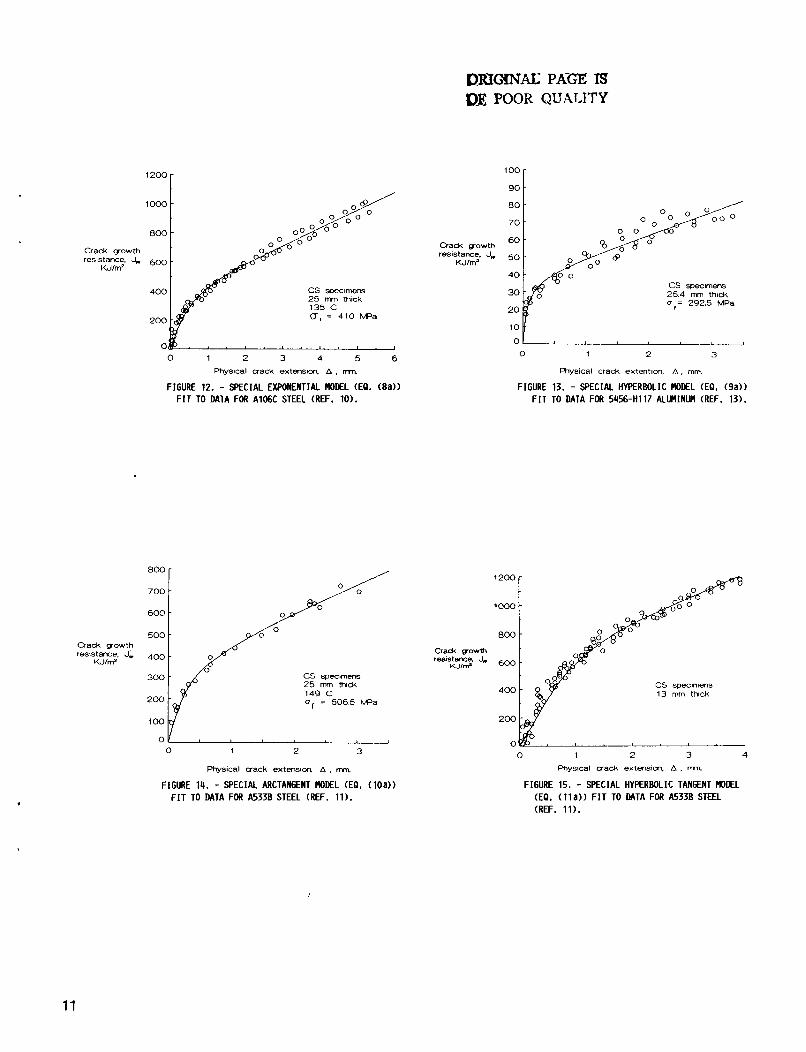
F igu res 12 to 15 were developed u s i n g equa t ions (8a) t o ( l l a ) . The f low s t r e s s was taken as t h e mean o f t h e r e p o r t e d y i e l d and u l t i m a t e s t r e n g t h s . F igu re 12 shows t h e s p e c i a l exponen t ia l model, equa t ion (8a) , f i t t o t h e same da ta as f i g u r e 7 . F i g u r e 13 shows t h e s p e c i a l h y p e r b o l i c model f i t t o da ta f o r 5456-H117 aluminum compact specimens ( r e f . 13) . F i g u r e 14 shows t h e spe- c i a l a r c t a n g e n t model f i t t o t h e same d a t a as f i g u r e 9. F i g u r e 15 shows t h e s p e c i a l h y p e r b o l i c t angen t model f i t t o t h e same d a t a as f i g u r e 10.

DISCUSSION

A l l p o s s i b l e combina t ions o f model equat ions and d a t a s e t s cannot be shown fo r space reasons. The combinat ions t h a t a r e p resented were chosen t o show t h a t each model i s a v i a b l e one. And indeed, each model i s a good f i t t o a t l e a s t one d a t a s e t .

For e l a s t i c R-curves, t he eye i s u s u a l l y a b l e t o judge whether a power model or an asympto t i c model i s a p p r o p r i a t e . Bu t t h e r e i s no obv ious way t o p r e d i c t which asympto t i c model w i l l be t h e b e s t f i t . For the e l a s t i c - p l a s t i c case, t h e r e a l s o i s no way t o t e l l i n advance whether t h e f low s t r e s s can be s p e c i f i e d or whether i t shou ld be a parameter t o be f i t t e d . t he 6 se ts o f JR data , t he b e s t f i t o v e r a l l was o b t a i n e d when t h e i n i t i a l s lope ( f low s t r e s s ) was f i t t e d r a t h e r than p r e s c r i b e d .

However, f o r 4 o f

6

CONCLUSIONS

I n summary, t h e i n s t a b i l i t y c a l c u l a t i o n method i s s i m p l e and e f f e c t i v e . The R-curve model e q u a t i o n s p resen ted h e r e a r e a l l v i a b l e , and a t l e a s t one o f them s h o u l d f i t a lmos t any d a t a . The e m p i r i c a l c o e f f i c i e n t s a r e e a s i l y e s t i - mated from a p l o t o f t h e raw d a t a and c o n v e r t e d from one system o f u n i t s t o a n o t h e r . I n comb ina t ion , t h e method and t h e models make p o w e r f u l tools f o r f r a c t u r e a n a l y s i s .

REFERENCES

1 .

2 .

3.

4.

5.

6.

7 .

8 .

9 .

10.

1 1 .

Creager, M. , i n F r a c t u r e Toughness E v a l u a t i o n by R-Curve Methods, ASTM STP-527, American S o c i e t y for T e s t i n g and M a t e r i a l s , P h i l a d e l p h i a , PA, 1973, pp. 105-112.

Newman, J.C., i n E l a s t i c - P l a s t i c F r a c t u r e Mechanics Technology, ASTM STP-896, J.C. Newman J r . and F.J. Loss, Eds., American S o c i e t y for T e s t i n g and M a t e r i a l s , P h i l a d e l p h i a , PA, 1985, pp. 5-96.

Orange, T.W., "Method f o r E s t i m a t i n g Crack-Ex tens ion Res is tance Curve from R e s i d u a l - S t r e n g t h Data, ' ' NASA TP-1753, N a t i o n a l A e r o n a u t i c s and Space A d m i n i s t r a t i o n , Washington, D.C., 1980.

Kumar, V . , German, M.D. , and Sh ih , C.F . , "An E n g i n e e r i n g Approach for E l a s t i c - P l a s t i c F r a c t u r e A n a l y s i s , " EPRI-NP-1931, E l e c t r i c Power Research I n s t i t u t e , 1981.

Wang, D.Y. , and McCabe, D.E. , i n Mechanics of Crack Growth, ASTM STP-590, American S o c i e t y for T e s t i n g and M a t e r i a l s , P h i l a d e l p h i a , PA, 1976, pp. 169-193.

Broek , D. , and V l i e g e r , H . , "The Th ickness E f f e c t i n P lane S t r e s s F r a c t u r e Toughness," NLR-TR-74032-U, N a t i o n a l Aerospace L a b o r a t o r y , The Ne the r lands , 1973.

Bluhm, J . I . , i n F r a c t u r e Mechanics o f A i r c r a f t S t r u c t u r e s , H . L i e b o w i t z , Ed., AGARDograph No. 176, AGARD, Neu i l l y -Sur -Se ine , France, 1973, pp. 74-88.

S c h r e i n e r , W . , Kramer, M . , K r i s c h e r , S . , and Langsam, Y . , PC Tech. J o u r n a l , Vol. 3, No. 5, May 1985, pp. 170-190.

Orange, T.W., " F r a c t u r e Toughness o f Wide 2014-T6 Aluminum Sheet a t -320 F," NASA TN D-4017, N a t i o n a l A e r o n a u t i c s and Space A d m i n i s t r a t i o n , Washington, D.C., 1967.

S u t t o n , G.E. , and V a s s i l a r o s , M.G., i n F r a c t u r e Mechanics: Seventeenth Volume, ASTM STP-905, J.H. Underwood, R. C h a i t , C.W. Smi th , D.P. Wilhem, W.A. Andrews, and J.C. Newman, Eds., American S o c i e t y for T e s t i n g and Mate- r i a l s , P h i l a d e l p h i a , PA, 1986, pp. 364-378.

C a r l s o n , K.W., and W i l l i a m s , J.A., i n F r a c t u r e Mechanics: T h i r t e e n t h Con- f e r e n c e , ASTM STP-743, R . Rober ts , Ed., American S o c i e t y for T e s t i n g and M a t e r i a l s , P h i l a d e l p h i a , PA, 1981 , pp. 503-524.

7

1 2 . V a s s i l a r o s , M.G., Hays, R . A . , and Gudas, J.P., i n F r a c t u r e Mechanics: Seventeenth Volume, ASTM STP-905, J.H. Underwood, R. C h a i t , C.W. Smith, D.P. Wilhem, W.A. Andrews, and J.C. Newman, Eds., American S o c i e t y for T e s t i n g and M a t e r i a l s , P h i l a d e l p h i a , PA, 1986, pp. 435-453.

Figure

3

4

5

6

7

13. Joyce J.A., and V a s s i l a r o s , M.G., i n F r a c t u r e Mechanics: T h i r t e e n t h Con- fe rence, ASTM STP-743, R. Rober ts , Ed., American S o c i e t y for T e s t i n g and M a t e r i a l s , P h i l a d e l p h i a , PA, 1981, pp. 525-542.

Equation Fitted equation

3 KR =

4

5

6 KR = 155.0(2/rr) arctan[(a/2)(A/15.06)1

7 KR = 158.6 tanh(A/13.76)

KR = 161.3C1 - exp(-A/l0.43)] KR = 50.98A/(0.9718 + A)

TABLE I. - ELASTIC R-CURVES

Figure

8

9

10

1 1

Equation Fitted equation

8 JR = (315.1 + 129.6A)Cl - exp(-A/0.3300)1 9 J R (357.7 + 3.600A)A/(5.172 + A)

10

1 1

J R = (373.5 + 130.7A)(2/~) arctan[(a/2)(A/0.3258)1

J R = (502.7 + 177.66) tanh(A/0.6318)

TABLE 11. - ELASTIC-PLASTIC R-CURVES

12

13

14

15

8a

9a

loa

lla

J R = (347.6 + 122.6A)Cl - exp(-A/0.4237)] J R = (38.87 + 13.00A)A/(O.O6645 + A) J R = (396.7 + 124.2A)(2/~) arctan(a/2)(A/0.2493)3 J R = (553.5 + 165.2A) tanh(A/0.8763)

8

Crack gowth

resistance

Crack mowth

resistance

OIUWAE PAGE IS OE POOR QUALITY

Crack growth

resistance

C. D. F. or H

I

Effective crack extenslm

FIGURE l ( a ) . - SCHEMATIC REPRESENTATION OF ELASTIC- ASYMPTOTIC R-CURVES (C, D, F, AND H ARE COEFFI- CIENTS I N EQS. (4) TO (7)).

Physical crack extension

FIGURE 2. - SCHEMTIC REPRESENTATION OF ELASTIC- PLASTIC R-CURVES (L, N, N, OR P ARE COEFFICIENT: I N EQS. (8) TO (11)).

Qadi CIowth 100 resistam. K.

W m -

40 CLW s p e c m s 1.5 mn thick

0 20 40 60 80 100

Effective crack extensi0n.A. nm

FIGURE 4. - EXPONENTIAL NOEL (EQ. (4)) F I T TO DATA FOR 7475-l761 ALUNINUN (REF. 5).

_ _ _ _ - - - - -

Mccu KKL

A w l i c m t 7 E ExpaxTltial 4 c Arct-t 6 D Hnmiwlc 5

Effective crack extenslo-

FIGURE l ( b ) . - ELASTIC ASW'TOTIC R-CURVES HAVING THE W E ASYMPTOTE AND INITIAL SLOPE.

MT) specimens 1.5 rrrn thick

10

0

0 5 10 15

Effective crack extension. A. mm

FIGURE 3. - POWER NODEL (EQ. ( 3 ) ) F I T TO DATA FOR 2014-T6 ALUNINUN (REF. 9).

2oi lo f

CS specimens 12.7 rnm thick

01 I

0 5 10 15 20 25 30 35 40 45 Effective crack extenion. A , mm.

FIGURE 5. - HYPERBOLIC NODEL (EO. ( 5 ) ) F I T TO DATA FOR 7075-T651 ALUNINUN (REF. 2).

9

Crack uowth resistance. K.,

Winn

OY . . . . . . . . I . . . . ,

0 50 100 150

Effective crack extension. A , mm.

FIGURE 6. - ARCTANGENT MODEL (EB. ( 6 ) ) F I T TO DATA FOR 2024-T3 A L M I N M (REF. 5 ) .

I2O0 I

Crack growm resistance. &

K J I d

0 I 2 3 5 6 Effective crack extmsion. A . nm

FIGURE 8. - MODIFIED EXPONENTIAL MODEL (EQ. (8)) FIT TO DATA FOR A106C STEEL (REF. 10).

180 - 0 0

00 Y " 0 n

Crack gowth 100 - resistance, K,

WinM

CLWL Specimens 1.5 mm tt-ick

Crack wowth resstawx.

K.!Jm'

0 20 40 60 80 100 Effective crack extension. A . mm.

FIGURE 7. - HYPERBOLIC TANGENT MODEL (EQ. (7)) FIT TO DATA FOR 7475-T761 ALMlNUM (REF. 5 ) .

500 r 400 -

300 -

200 - cs specimens 12.7 nrn ttnck

0 0 10 20 30 40

Physical crack extensirn A . mn

FIGURE 9. - MODIFIED HYPERBOLIC MODEL (EQ. (9)) F I T TO DATA FOR 2024-T351 ALMINUN (REF. 2) .

' .

800 1400

1200 700

600 1000

500 Crack gowm Crack gowth reslstare. JI resistme. J, 4~~ K J d

600 CS specimens

149 C

KJ/rn'

300 25 rnrn thick

200

100 200

0 0

400 CS Specimens 13 nm thick

0 1 2 3 4 0 1 2 3 4

Physical crack extension. A , nrn Physical crack extensim A , mn

FIGURE 10. - MODIFIED ARCTANGENT MODEL FIGURE 11. - MODIFIED HYPERBOLIC TANGENT MODEL (EQ. (10)) F IT TO DATA FOR A5336 STEEL (REF. 11). (REF. 12).

(EQ. (11)) F IT TO DATA FOR A106B STEEL

I 10 D ! m A L PAGE IS

POOR QUALITY

DEIGTI'4A.G PAGE IS DE POOR QUALITY

Crack gowth resistance. 4

KJ/rn'

Crack gowth resistince. J,

KJIrn'

.

I2Oo r 1000

aoo

600

400 cs SPeClmens 25 nm mock 135 C 0, = 4 1 0 W a 200

0 0 1 2 3 4 5 6

Physical crack extmsim A , mn

FIGURE 12. - SPECIAL EXPONENTIAL MODEL (EP. (8a)) FIT TO DATA FOR A106C STEEL (REF. 10).

700

400 500 t o /

600 c CS weamens 25 krn ttw=k 149 C U f = 506.5 Wa

100

0 1 2 3

Physical crack extensim A . mn

FIGURE 14. - SPECIAL ARCTANGENT NODEL (EP. (loa)) FIT TO DATA FOR A533B STEEL (REF. 11) .

Crack gowth resistance. J,

KJlm'

Crack wow* resistance. J.

Wlm'

100

901 80

70

60

50

40 CS Specimens

30 25.4 mm thick u = 292.5 MPa

20

01 0 1 2 3

Physical crack extention. A . rnm.

FIGURE 13. - SPECIAL HYPERBOLIC MODEL (EQ, (9a)) FIT TO DATA FOR 5456-H117 ALURINIJN (REF. 13).

1200

1000

800

600

400

200

0

CS specimens 13 mm thick

0 1 2 3 4 Physical crack extensim A , nm

FIGURE 15. - SPECIAL HYPERBOLIC TANGENT MODEL (EP. ( l l a ) ) FIT TO DATA FOR A5338 STEEL (REF. 1 1 ) .

I

11

Report Documentation Page

NASA TM-100935 4. Title and Subtitle

Space AdminisIratian

1. Report No. I 2. Government Accession No. I 3. Recipient’s Catalog No,

5. Report Date

7. Author@)

Thomas W . Orange

Method and Models for R-Curve Instability Cal cu 1 at i on s

8. Performing Organization Report No.

E-42 1 2 10. Work Unit No.

6. Performing Organization Code 6

7. Key Words (Suggested by Author@))

R-curve; J-R curves; Instability; ,Elastic-plastic fracture; Fracture tests; Data reduction; Mathematical model s

18. Distribution Statement

Unclassified - Unlimited Subject Category 39

505-63-81 11. Contract or Grant No.

9. Performing Organization Name and Address

National A,eronautics and Space Administration Lewis Research Center Cleveland, Ohio 44135-3191 13. Type of Report and Period Covered

3. Security Classif. (of this report) 20. Security Classif. (of this page)

Uncl ass i f i ed Uncl assi f i ed

2. Sponsoring Agency Name and Address

21. No of pages 22. Price’

12 A02

National Aeronautics and Space Administration Washington, D.C. 20546-0001

Technical Memorandum

I

5. Supplementary Notes

Prepared for the Twenty-First National Symposium on Fracture Mechanics, spon- sored by the American Society for Testing and Materials, Annapolis, Maryland, June 28-30, 1988.

6. Abstract

This paper presents a simple method for performing elastic R-curve instability calculations. For a single material-structure combination, the calculations can be done on some pocket calculators. the development of a comprehensive program having libraries of driving force equations for different configurations and R-curve model equations for different materials. The paper also presents several model equations for fitting to exper- imental R-curve data, both linear elastic and elastoplastic. The models are fit to data from the literature to demonstrate their viability.

On microcomputers and larger, it enables