Meteorological Path Planning Using Dynamic Programming … · Meteorological Path Planning Using...
11
1 Meteorological Path Planning Using Dynamic Programming for a Solar-Powered UAV Lukas Wirth 1 , Philipp Oettershagen 1 , Jacques Ambühl 2 , Roland Siegwart 1 1 ETH Zurich Autonomous Systems Lab Leonhardstrasse 21 8092 Zurich +41 44 632 7395 [email protected] 2 Federal Office of Meteorology and Climatology MeteoSwiss Operation Center 1, Postfach 257 CH-8058 Zurich-Airport +41 79 278 2540 [email protected] Abstract—Solar-powered Unmanned Aerial Vehicles (SUAV) designed for Low-Altitude Long-Endurance (LALE) applications provide potential multi-day continuous flight capability, but are generally prone to local meteorological impediments such as rain, strong winds or reduced solar irradiance. This paper therefore presents METPASS, the Meteorology-aware Trajectory Planning and Analysis Software for Solar-powered UAVs. METPASS optimizes large- scale solar-powered UAV missions using a detailed consideration of meteorological effects: An optimal trajectory is found on a 3-D grid for given departure and arrival points by applying a Dynamic Programming approach and a cost function that considers environmental hazards, winds, solar radiation, aircraft parameters and flight time. The cost function is evaluated based on a kinematic and energetic UAV system model and forecast data from the European Centre for Medium-Range Weather Forecasts (ECMWF). The trajectory- planning environment is applied to an envisioned fully autonomous and solar-powered crossing of the North Atlantic Ocean by AtlantikSolar, a 5.6m-wingspan SUAV developed at ETH Zurich. Results based on historical ECMWF weather data from 2012 and 2013 show that properly pre-optimized routes allow the Atlantic crossing even in case of significant global cloud coverage and that optimal routes can reduce the required flight time by up to 50% (from 106h to 52h) by exploiting wind conditions. TABLE OF CONTENTS 1. INTRODUCTION ................................................. 1 2. METHODOLOGY AND IMPLEMENTATION......... 2 3. FUNCTIONAL VALIDATION AND PARAMETER REFINEMENT ........................................................ 5 4. RESULTS............................................................ 7 5. CONCLUSION..................................................... 9 REFERENCES......................................................... 9 BIOGRAPHY ........................................................ 10 1. INTRODUCTION Solar-powered Unmanned Aerial Vehicles Today’s solar-powered Unmanned Aerial Vehicles (SUAV) combine highly-optimized airframes and solar-powered recharging systems to provide increased flight-endurance. They can be designed to provide multi-day continuous flight - often termed perpetual-flight - as recently shown by the 3.2m-wingspan SkySailor [1] and Zephyr [2]. These demonstrations, together with ongoing technical improvements in solar cell, electrical propulsion and battery technology have focused attention on SUAVs and their application in Search and Rescue (SAR) missions, meteorological observations, wildfire detection and the creation of communication networks. High-Altitude Long- Endurance (HALE) platforms functioning as low-cost atmospheric satellites have created growing interest among IT companies by providing a solution to the latter applications [3]. In contrast, Low-Altitude Long-Endurance (LALE) solar-powered UAVs are more suitable for SAR missions due to lower complexity, size and thus hand- launch capability. Within this scope, ETH Zurich is currently developing AtlantikSolar [4], a solar-powered LALE-UAV platform with the goal to provide multi-day continuous flight even under partially cloudy conditions and to demonstrate the performance by performing an Atlantic crossing in summer 2015. The aircraft and its specifications are presented in Figure 1 and Table 1. However, a major challenge for SUAVs consists of their sensitivity to environmental conditions caused by their lightweight design, low airspeed and dependency on solar radiation. The capability to perform detailed mission pre- Table 1. AtlantikSolar UAV specifications Wingspan 5.65 m Weight 7 kg Solar module area 1.4 m 2 Battery total energy 700 Wh Typical power consumption 50 W Typical airspeed 9 m/s
Transcript of Meteorological Path Planning Using Dynamic Programming … · Meteorological Path Planning Using...

1
Meteorological Path Planning Using Dynamic
Programming for a Solar-Powered UAV Lukas Wirth
1, Philipp Oettershagen
1, Jacques Ambühl
2, Roland Siegwart
1
1ETH Zurich
Autonomous Systems Lab Leonhardstrasse 21
8092 Zurich +41 44 632 7395
2Federal Office of Meteorology and
Climatology MeteoSwiss Operation Center 1, Postfach 257
CH-8058 Zurich-Airport +41 79 278 2540
Abstract—Solar-powered Unmanned Aerial Vehicles (SUAV)
designed for Low-Altitude Long-Endurance (LALE)
applications provide potential multi-day continuous flight
capability, but are generally prone to local meteorological
impediments such as rain, strong winds or reduced solar
irradiance. This paper therefore presents METPASS, the
Meteorology-aware Trajectory Planning and Analysis
Software for Solar-powered UAVs. METPASS optimizes large-
scale solar-powered UAV missions using a detailed
consideration of meteorological effects: An optimal trajectory
is found on a 3-D grid for given departure and arrival points
by applying a Dynamic Programming approach and a cost
function that considers environmental hazards, winds, solar
radiation, aircraft parameters and flight time. The cost
function is evaluated based on a kinematic and energetic UAV
system model and forecast data from the European Centre for
Medium-Range Weather Forecasts (ECMWF). The trajectory-
planning environment is applied to an envisioned fully
autonomous and solar-powered crossing of the North Atlantic
Ocean by AtlantikSolar, a 5.6m-wingspan SUAV developed at
ETH Zurich. Results based on historical ECMWF weather
data from 2012 and 2013 show that properly pre-optimized
routes allow the Atlantic crossing even in case of significant
global cloud coverage and that optimal routes can reduce the
required flight time by up to 50% (from 106h to 52h) by
exploiting wind conditions.
TABLE OF CONTENTS
1. INTRODUCTION ................................................. 1
2. METHODOLOGY AND IMPLEMENTATION ......... 2 3. FUNCTIONAL VALIDATION AND PARAMETER
REFINEMENT ........................................................ 5 4. RESULTS ............................................................ 7
5. CONCLUSION ..................................................... 9 REFERENCES ......................................................... 9 BIOGRAPHY ........................................................ 10
1. INTRODUCTION
Solar-powered Unmanned Aerial Vehicles
Today’s solar-powered Unmanned Aerial Vehicles (SUAV)
combine highly-optimized airframes and solar-powered
recharging systems to provide increased flight-endurance.
They can be designed to provide multi-day continuous flight
- often termed perpetual-flight - as recently shown by the
3.2m-wingspan SkySailor [1] and Zephyr [2]. These
demonstrations, together with ongoing technical
improvements in solar cell, electrical propulsion and battery
technology have focused attention on SUAVs and their
application in Search and Rescue (SAR) missions,
meteorological observations, wildfire detection and the
creation of communication networks. High-Altitude Long-
Endurance (HALE) platforms functioning as low-cost
atmospheric satellites have created growing interest among
IT companies by providing a solution to the latter
applications [3]. In contrast, Low-Altitude Long-Endurance
(LALE) solar-powered UAVs are more suitable for SAR
missions due to lower complexity, size and thus hand-
launch capability. Within this scope, ETH Zurich is
currently developing AtlantikSolar [4], a solar-powered
LALE-UAV platform with the goal to provide multi-day
continuous flight even under partially cloudy conditions and
to demonstrate the performance by performing an Atlantic
crossing in summer 2015. The aircraft and its specifications
are presented in Figure 1 and Table 1.
However, a major challenge for SUAVs consists of their
sensitivity to environmental conditions caused by their
lightweight design, low airspeed and dependency on solar
radiation. The capability to perform detailed mission pre-
Table 1. AtlantikSolar UAV specifications
Wingspan 5.65 m
Weight 7 kg
Solar module area 1.4 m2
Battery total energy 700 Wh
Typical power consumption 50 W
Typical airspeed 9 m/s
2
Figure 1 – The AtlantikSolar UAV
planning with respect to meteorological conditions is
therefore indispensable for successful long-term operation
of solar-powered UAVs.
Contributions of this paper
This paper contributes the Meteorology-aware Trajectory
Planning and Analysis Software for Solar-powered UAVs
(METPASS) developed at ETH Zurich to optimize large-
scale UAV missions with respect to flight safety and user-
definable performance-metrics (e.g. flight-time) by tightly
integrating the UAV system model with meteorological
considerations. METPASS integrates
1) A Dynamic Programming (DP) [15] optimization
algorithm based on [5] that is extended to provide
trajectory-optimization in altitude.
2) A cost function that defines trajectory-optimality
by weighing safety (wind, rain, thunderstorms) and
performance metrics.
3) A kinematic and energetic system model for solar-
powered UAVs.
4) Methods to directly incorporate meteorological
forecast data from the European Centre for
Medium-Range Weather Forecasts (ECMWF).
By employing these components, METPASS allows to
consider all aspects required for the safe operation of
SUAVs. Feasibility analysis based on historical data,
mission preplanning and in-flight path corrections can be
performed. In contrast, previous literature addressed only
individual aspects in mostly simplified conditions. In [6],
minimization of flight time and fuel consumption in real
wind conditions is addressed. As a fuel-powered UAV is
considered, environmental impediments and solar radiation
are not taken into account. [7] and [8] address the
maximization of solar power generation in theoretical
situations without any consideration of meteorological data.
[9] and [10] investigate path optimization with respect to
military threats or restricted areas.
2. METHODOLOGY AND IMPLEMENTATION
Overview
The path optimization problem solved by METPASS can be
stated as follows: Given fixed departure and arrival
coordinates, find a path and departure time which minimizes
the total cost as defined by a cost function. The cost
function includes environmental conditions such as solar
radiation or precipitation as well as aircraft parameters like
power consumption or State of Charge (SoC).
Environmental conditions are estimated based on time-
varying ECMWF forecast data in a three-dimensional grid.
The system model includes flight kinematics with respect to
horizontal wind, power generation through the solar
modules and the power consumption of the aircraft. The
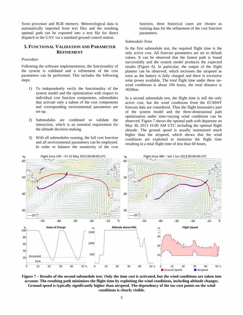
required system components, namely the basic optimization
algorithm, the cost function, the forecast data and the system
Figure 2 – Overview of the optimization software and
the required components
model are explained in detail in the following sections. A
graphical overview is given in Figure 2.
Optimization Algorithm
The optimization algorithm is an extended version of the
Dynamic Programming based algorithm presented in [5]
with the altitude as an additional optimization variable. The
working principle can be shown on a basic example, where
the goal is to find the shortest distance between Bell Island
(CA) and Lisbon (PT) (Figure 3). In a first step, a three-
dimensional grid, connecting the departure and arrival
points, is generated. The grid is horizontally divided into i
slices of j vertices, and vertically into k levels. More
information about scaling and resolution of the grid can be
found in [14]. Starting from the departure node, the cost (in
this example the travel distance) to each subsequent node is
calculated and stored. Then, starting from the nodes in the
third slice of the grid, the DP algorithm
𝑑𝑖,𝑗,𝑘 = minn∈slicei−1[di−1,n + ∆i−1,n
i,j,k] (1)
is applied to find the shortest total distance 𝑑𝑖,𝑗,𝑘 from the
departure point to each node of the grid. This is done by
minimizing the sum of the a priori known distances di−1,n
and the corresponding additional travel distance ∆i−1,ni,j,k
. A
decision tree consisting of globally optimal sub routes is
thus built up which finally reaches the arrival point. The
Figure 3 – Exemplary application of the optimization
algorithm to a shortest path problem. The decision grid,
optimal route
cost function
initial conditions
meteorologicalforecast data
decision grid
departure/arrivalcoordinates
decision tree
system model
iso cost lines
route information
60 50 40 30 20 1030
35
40
45
50
55
i
j
°E
°N
-10-20-30-40-50-60
50
45
40
35 𝑑𝑖,𝑗,𝑘 = minn∈slicei−1
[di−1,n + ∆i−1,n
i,j,k ]

3
decision tree, a highlighted node and the resulting
shortest path from Canada to Portugal are also shown.
optimal path can then be extracted by going back up the tree
from the arrival point.
In contrast to this simplified example, in which the cost is
represented by the Euclidean distance that is calculated
analytically as described in [5], the evaluation of the real
cost function depends on high-resolution time-varying
forecast data and an advanced system model. Thus the flight
on each path segment needs to be simulated using numerical
integration, which is a main expansion compared to [5],
where the system model only consists of a polar diagram.
Cost Function
The cost function is a weighted combination of flight time,
environmental costs and system costs. The environmental
costs indicate an environmental threat to the airplane, which
can be directly derived from the forecast data. This includes
strong wind, wind gusts, humidity, precipitation and
thunderstorms. The system costs are SoC, power
consumption and power generation. To allow for a
consistent summation and weighting, each of the costs Ck is
expressed through
Ck = H(x) ∙exp(
xk−αkβk−αk
∙εk)−1
exp(εk)−1 . (2)
This normalizes every cost and allows to adjust its influence
on the total cost using the parameters αk, βk and εk. The
parameters αk and βk define the lower threshold and the
upper limit, where the generated cost is bounded. By using
the Heaviside function H(x), values xk below the threshold
generate no cost, as they are not in a critical range and do
not need to be considered. Values above the limit are
considered as too dangerous for the aircraft and every
violation will lead to a cancellation of the corresponding
path. The exponent εk determines the shape of the cost
curve as illustrated in Figure 4.
Figure 4 – Cost Function Example
The accumulated cost for a path segment is finally
calculated by summing up all 9 costs to a total cost and
integrating it over the flight time, as defined by
𝐶 = ∫ ∑ Ck9𝑘=1
𝑡2𝑡1
𝑑𝑡 . (3)
Meteorological forecast data
The meteorological data is obtained from ECMWF as
historical data from 2012 to 2013. A horizontal resolution of
0.125° with five altitude levels between 0 and 1600m above
sea-level and a time step of 6 hours are used. Additionally,
forecast data with up to 5 days forecast range and a 3 hour
time-step is available, which is updated every 12 hours. The
data is linearly interpolated in all three spatial dimensions as
well as time1. The used parameters are listed in Table 2. A
more detailed description of how they are applied to the cost
function and the system model can be found in [14].
Table 2. Forecast Parameters received from ECMWF
Parameter Unit Description Altitude
dependent
Temperature °C Yes
Relative humidity % Yes
Zonal wind m/s Horizontal wind
from West to East Yes
Meridional wind m/s Horizontal wind
from South to North Yes
Wind gusts m/s Max. wind gust in
the last time step No
Total precipitation mm Accumulated over
last time step No
Convective available
potential energy J/kg
Causing updrafts
and thunderstorms No
Total solar radiation
(direct + diffuse) J/m2
Accumulated over last time step
No
Direct solar
radiation J/ m2
Accumulated over
last time step No
System Model
An overview of the system model is given in Figure 5. The
main components are the power balance estimation,
including the evaluation of solar power generation, system
power consumption and SoC, and the flight kinematics with
respect to wind speed and airspeed. The flight planner
represents the decision logic of the UAV, which determines
the airspeed of the aircraft depending on the system state.
The airspeed may be increased in presence of strong
headwind in order to maintain a certain ground speed or if
there is excessive solar power available, the battery is
already fully charged and the aircraft is not allowed to gain
additional altitude. For the calculation of the power
generation, direct and diffuse solar radiation are considered
separately. The incident angle of the direct radiation is
1 The solar radiation is an exception as it changes much faster than all other
meteorological parameters, which cannot be sufficiently tracked by a 3-
hour time step. The model-based estimation of current radiation values is described in [14].
0 2 4 6 8 10precipitation0.0
0.2
0.4
0.6
0.8
1.0
Precipitation cost
Threshold 1 Limit 10
cost [-] Precipitation Cost
precipitation [mm/6h]
exponent
0.5
5
12
34
threshold=1
limit=10
0 2 4 6 8 100.0
0.2
0.4
0.6
0.8
1.0

4
calculated for every solar module using the solar radiation
models presented in [11], [12] and [14] under consideration
of the aircraft geometry. The radiation onto the surface is
then calculated using the cosine of the incidence angle. For
the diffuse part of the radiation, the surface is assumed to be
horizontal and thus the incidence angle is neglected. With
Figure 5 – Overview of the system model
the total area 𝐴 of the solar modules and the efficiencies of
the solar cells 𝜂𝑐𝑒𝑙𝑙 and the Maximum Power Point Trackers
ηMPPT, the total incoming power is
Psolar = (Idiff + Idirect ∙ cosφ) ∙ A ∙ ηcell ∙ ηMPPT . (4)
The overall level-flight power consumption of the UAV
depends on airspeed 𝑣 and altitude and thus air density 𝜌. It
is generally given by
𝑃𝑙𝑒𝑣𝑒𝑙(𝜌, 𝑣) =𝑃𝑝𝑟𝑜𝑝(ρ,𝑣)
𝜂𝑝𝑟𝑜𝑝(𝜌,𝑣)+ 𝑃𝑎𝑣 + 𝑃𝑝𝑙𝑑 , (5)
where 𝑃𝑝𝑟𝑜𝑝 𝜂𝑝𝑟𝑜𝑝⁄ determines the required electrical
propulsion power, and 𝑃𝑎𝑣 and 𝑃𝑝𝑙𝑑 are avionics and
payload power respectively. In our case, the dependence of
𝑃𝑙𝑒𝑣𝑒𝑙 on the airspeed 𝑣 is modelled through
Plevel(ρ0, 𝑣) = C2 ∙ v2 + C1 ∙ v + C0 , (6)
which is identified directly from AtlantikSolar power
measurement test flights performed at constant altitude and
thus air density 𝜌0. The scaling to different altitudes or air
densities is done according to [13] using
𝑃𝑙𝑒𝑣𝑒𝑙(𝜌, 𝑣) = √𝜌0
𝜌∙ [𝐶2 ∙ 𝑣
2 ∙𝜌
𝜌0+ 𝐶𝑃1 ∙ 𝑣 ∙ √
𝜌
𝜌0+ 𝐶0] . (7)
With regard to the climb rate ℎ, the total flight power 𝑃𝑓𝑙𝑖𝑔ℎ𝑡
is given by
𝑃𝑓𝑙𝑖𝑔ℎ𝑡(𝜌, 𝑣) = 𝑃𝑙𝑒𝑣𝑒𝑙(𝜌, 𝑣) +𝑚∙𝑔∙ℎ
𝜂𝑐𝑙𝑖𝑚𝑏 , (8)
with the airplane mass 𝑚 and the climbing efficiency 𝜂𝑐𝑙𝑖𝑚𝑏 .
The SoC is updated based on the power balance given by
𝑆𝑜𝐶 =𝑃𝑠𝑜𝑙𝑎𝑟−𝑃𝑓𝑙𝑖𝑔ℎ𝑡
𝐸𝑏𝑎𝑡𝑡𝑒𝑟𝑦∙ 𝜂𝑐ℎ𝑎𝑟𝑔𝑒 , (9)
with the total energy of the battery 𝐸𝑏𝑎𝑡𝑡𝑒𝑟𝑦 and the battery
efficiency 𝜂𝑐ℎ𝑎𝑟𝑔𝑒 .
The flight kinematics include calculation of the wind
correction angle and the resulting ground speed. More
information about the system model may be found in [14].
Implementation
The implementation of the METPASS software, including
data import and a versatile GUI, is done in Mathematica.
The main optimization algorithm runs as compiled C code
for the purpose of speed with full multicore support.
Calculation times between 10 and 20 minutes are achieved
for the cases presented in this paper with a quad-core Intel
0 20 40 60 80 100
h0
5
10
15
20
m
s
Flight speed
airspeed groundspeed
0 20 40 60 80 100
h
50
0
50
100
150
200
W
Power
level flight power consumption solar power income
battery charge power change of potential energy
excessive power consumption
100
80
60
40
20
%
0 20 40 60 80 100 h 0 20 40 60 80 100 h 0 20 40 60 80 100 h
State of Charge Flight Speed(Airspeed = Ground Speed)
Power
5
10
15
20
𝑚
-50
0
50
100
150
200
W
𝑃𝑙𝑒𝑣𝑒𝑙 (=𝑃𝑓𝑙𝑖𝑔ℎ𝑡)𝑃 𝑜𝑙𝑎𝑟𝑃 𝑜𝑙𝑎𝑟 − 𝑃𝑓𝑙𝑖𝑔ℎ𝑡
threshold
limit
Figure 6 – Results of the first submodule test (2D, no altitude changes): Only the time cost is activated and all
meteorological parameters are set to default values. The decision tree and the shortest path are calculated. The
purple iso-cost points build a circle around the departure point. SoC and power consumption fluctuate periodically
and the airspeed is increased if there is excessive solar power available and the battery fully charged.
°E
°N
50
45
40
35-50 -40 -30 -20 -10
Decision Tree
Iso-cost Points
Motor+ -
flightplanner
ECMWF Forecast data
ground speedradiation
wind
Electronics
airspeed
SoC
solar power
power consumption
αwind
βground speed
airspeed
5
Xeon processor and 8GB memory. Meteorological data is
automatically imported from text files and the resulting
optimal path can be exported into a text file for direct
dispatch to the UAV via a standard ground control station.
3. FUNCTIONAL VALIDATION AND PARAMETER
REFINEMENT
Procedure
Following the software implementation, the functionality of
the system is validated and a refinement of the cost
parameters can be performed. This includes the following
steps:
1) To independently verify the functionality of the
system model and the optimization with respect to
individual cost function components, submodules
that activate only a subset of the cost components
and corresponding environmental parameters are
set-up.
2) Submodules are combined to validate the
interaction, which is an essential requirement for
the altitude decision-making.
3) With all submodules running, the full cost function
and all environmental parameters can be employed.
In order to balance the sensitivity of the cost
function, three historical cases are chosen as
training data for the refinement of the cost function
parameters.
Submodule Tests
In the first submodule test, the required flight time is the
only active cost. All forecast parameters are set to default
values. It can be observed that the fastest path is found
successfully and the system model produces the expected
results (Figure 6). In particular, the output of the flight
planner can be observed, which increases the airspeed as
soon as the battery is fully charged and there is excessive
solar power available. The total flight time under these no-
wind conditions is about 106 hours, the total distance is
3650km.
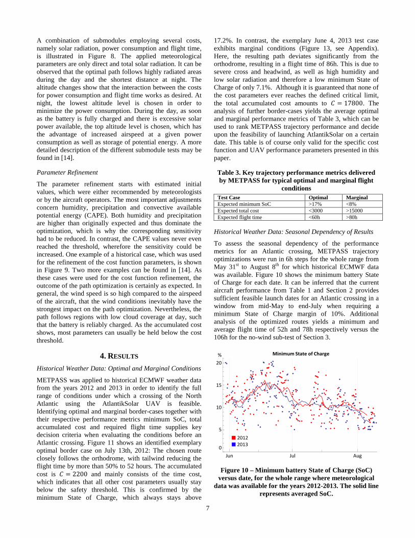
In a second submodule test, the flight time is still the only
active cost, but the wind conditions from the ECMWF
forecast data are considered. Thus the flight kinematics part
of the system model and the three-dimensional path
optimization under time-varying wind conditions can be
observed. Figure 7 shows the optimal path with departure on
May 30, 2013 10.00 AM UTC including the optimal flight
altitude. The ground speed is usually maintained much
higher than the airspeed, which shows that the wind
conditions are exploited to minimize the flight time
resulting in a total flight time of less than 60 hours.
20 m
s
50 40 30 20 1025
30
35
40
45
50
55
60
Wind on Fri 31 May 2013 00:00:00UTC
Flight time: 14h UTC: Fri 31 May 2013 00:00:00 Local time: Thu 30 May 2013 21:39:21
20 𝑚𝑠
-10-20-30-40-50 °E
30
40
50
60°N Flight time 14h – Fri 31 May 2013 00:00:00 UTC
20 m
s
50 40 30 20 1025
30
35
40
45
50
55
60
Wind on Sat 1 Jun 2013 00:00:00UTC
Flight time: 38h UTC: Sat 1 Jun 2013 00:00:00 Local time: Fri 31 May 2013 23:10:48
20 𝑚𝑠
30
40
50
60°N
-10-20-30-40-50 °E
Flight time 38h – Sat 1 Jun 2013 00:00:00 UTC
0 10 20 30 40 50
h0
5
10
15
20
25
30
35
m
s
Flight speed
airspeed groundspeed
0 10 20 30 40 50h
500
1000
1500
m
Altitude above sealevel
0 10 20 30 40 50 h 0 10 20 30 40 50 h 0 10 20 30 40 50 h
100
80
60
40
20
% State of Charge Altitude above MSL Flight Speed
Ground Speed Airspeed
m
1500
1000
500
20
10
30
𝑚
threshold
limit
Figure 7 – Results of the second submodule test: Only the time cost is activated, but the wind conditions are taken into
account. The resulting path minimizes the flight time by exploiting the wind conditions, including altitude changes.
Ground speed is typically significantly higher than airspeed. The dependency of the iso-cost points on the wind
conditions is clearly visible.

6
Figure 8 – Combination of submodules: Considered costs are solar radiation, power consumption and flight time.
Only the weather parameters direct and total radiation are taken into account. The altitude changes depending on the
SoC. The iso-cost points illustrate the influence of the radiation on the total cost.
Figure 9 – Result of the historical case used for parameter refinement: The chosen path exploits wind conditions while
providing enough solar radiation to fully charge the battery. The accumulated cost plot shows which cost parameters
exceed the threshold. Only the time cost is constantly increasing.
0 20 40 60 80 100h
500
1000
1500
m
Altitude above sealevel
0 20 40 60 80 100
h0
10
20
30
40
50
m
s
Flight speed
airspeed groundspeed
0 20 40 60 80 100 h
100
80
60
40
20
% State of Charge Altitude above MSL Flight Speed(Airspeed = Ground Speed)
m
1500
1000
500
20
10
30
𝑚
0 20 40 60 80 100 h
threshold
limit
0 20 40 60 80 100 h
0 10 20 30 40 50 60
h0
200
400
600
800
1000
W
m2
Global radiation on horizontal surface
total direct clear sky
0 10 20 30 40 50 60
h0
1000
2000
3000
4000
_
Accumulated general cost
time SoC power cons . rad . factor environmental
100
80
60
40
20
% State of Charge Global Radiation on Horizontal Surface Accumulated Costs
threshold
limit
0 10 20 30 40 50 60 h 0 10 20 30 40 50 60 h0 10 20 30 40 50 60 h
4000
3000
2000
1000
0
[-]
SoCPower Consumption
TimeEnvironment
Radiation
800
600
400
200
0
𝑚2
Total Direct Clear-sky
30
40
50
60°N
-10-20-30-40-50 °E
Flight time 39h – Mon 21 Apr 2014 18:00:00 UTC
50 40 30 20 1025
30
35
40
45
50
55
60
Average total global radiation over last 3 hours on Mon 21 Apr 2014 18:00:00UTC
Flight time: 39h UTC: Mon 21 Apr 2014 18:00:00 Local time: Mon 21 Apr 2014 15:24:11
50 40 30 20 1025
30
35
40
45
50
55
60
Average total global radiation over last 3 hours on Wed 23 Apr 2014 18:00:00UTC
Flight time: 87h UTC: Wed 23 Apr 2014 18:00:00 Local time: Wed 23 Apr 2014 16:36:00
30
40
50
60°N
-10-20-30-40-50 °E
Flight time 87h – Wed 23 Apr 2014 18:00:00 UTCW
m2
600
800
1000
1200
0
200
400
20 m
s
60 50 40 30 20 10
30
40
50
60
Total cloud cover on Fri 1 Jun 2012 00:00:00UTC
Flight time: 14h UTC: Fri 1 Jun 2012 00:00:00 Local time: Thu 31 May 2012 21:02:40
20 m
s
60 50 40 30 20 10
30
40
50
60
Total cloud cover on Sat 2 Jun 2012 12:00:00UTC
Flight time: 50h UTC: Sat 2 Jun 2012 12:00:00 Local time: Sat 2 Jun 2012 10:41:52
30
40
50
60°N
-10-20-30-40-50 °E-60
20 𝑚𝑠
30
40
50
60°N
-10-20-30-40-50 °E-60
20 𝑚𝑠
Flight time 14h – Fri 1 Jun 2012 00:00:00 UTC Flight time 50h – Sat 2 Jun 2012 12:00:00 UTC
7
A combination of submodules employing several costs,
namely solar radiation, power consumption and flight time,
is illustrated in Figure 8. The applied meteorological
parameters are only direct and total solar radiation. It can be
observed that the optimal path follows highly radiated areas
during the day and the shortest distance at night. The
altitude changes show that the interaction between the costs
for power consumption and flight time works as desired. At
night, the lowest altitude level is chosen in order to
minimize the power consumption. During the day, as soon
as the battery is fully charged and there is excessive solar
power available, the top altitude level is chosen, which has
the advantage of increased airspeed at a given power
consumption as well as storage of potential energy. A more
detailed description of the different submodule tests may be
found in [14].
Parameter Refinement
The parameter refinement starts with estimated initial
values, which were either recommended by meteorologists
or by the aircraft operators. The most important adjustments
concern humidity, precipitation and convective available
potential energy (CAPE). Both humidity and precipitation
are higher than originally expected and thus dominate the
optimization, which is why the corresponding sensitivity
had to be reduced. In contrast, the CAPE values never even
reached the threshold, wherefore the sensitivity could be
increased. One example of a historical case, which was used
for the refinement of the cost function parameters, is shown
in Figure 9. Two more examples can be found in [14]. As
these cases were used for the cost function refinement, the
outcome of the path optimization is certainly as expected. In
general, the wind speed is so high compared to the airspeed
of the aircraft, that the wind conditions inevitably have the
strongest impact on the path optimization. Nevertheless, the
path follows regions with low cloud coverage at day, such
that the battery is reliably charged. As the accumulated cost
shows, most parameters can usually be held below the cost
threshold.
4. RESULTS
Historical Weather Data: Optimal and Marginal Conditions
METPASS was applied to historical ECMWF weather data
from the years 2012 and 2013 in order to identify the full
range of conditions under which a crossing of the North
Atlantic using the AtlantikSolar UAV is feasible.
Identifying optimal and marginal border-cases together with
their respective performance metrics minimum SoC, total
accumulated cost and required flight time supplies key
decision criteria when evaluating the conditions before an
Atlantic crossing. Figure 11 shows an identified exemplary
optimal border case on July 13th, 2012: The chosen route
closely follows the orthodrome, with tailwind reducing the
flight time by more than 50% to 52 hours. The accumulated
cost is 𝐶 = 2200 and mainly consists of the time cost,
which indicates that all other cost parameters usually stay
below the safety threshold. This is confirmed by the
minimum State of Charge, which always stays above
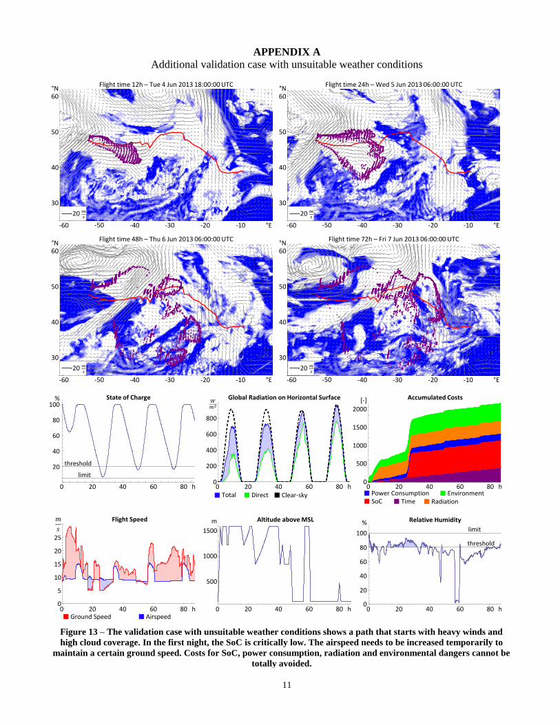
17.2%. In contrast, the exemplary June 4, 2013 test case
exhibits marginal conditions (Figure 13, see Appendix).
Here, the resulting path deviates significantly from the
orthodrome, resulting in a flight time of 86h. This is due to
severe cross and headwind, as well as high humidity and
low solar radiation and therefore a low minimum State of
Charge of only 7.1%. Although it is guaranteed that none of
the cost parameters ever reaches the defined critical limit,
the total accumulated cost amounts to 𝐶 = 17800. The
analysis of further border-cases yields the average optimal
and marginal performance metrics of Table 3, which can be
used to rank METPASS trajectory performance and decide
upon the feasibility of launching AtlantikSolar on a certain
date. This table is of course only valid for the specific cost
function and UAV performance parameters presented in this
paper.
Table 3. Key trajectory performance metrics delivered
by METPASS for typical optimal and marginal flight
conditions
Test Case Optimal Marginal
Expected minimum SoC >17% <8%
Expected total cost <3000 >15000
Expected flight time <60h >80h
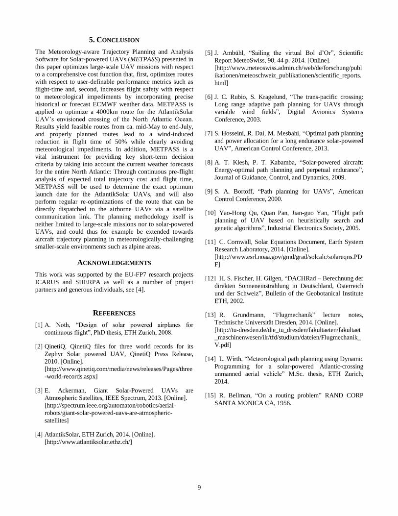
Historical Weather Data: Seasonal Dependency of Results
To assess the seasonal dependency of the performance
metrics for an Atlantic crossing, METPASS trajectory
optimizations were run in 6h steps for the whole range from
May 31st to August 8
th for which historical ECMWF data
was available. Figure 10 shows the minimum battery State
of Charge for each date. It can be inferred that the current
aircraft performance from Table 1 and Section 2 provides
sufficient feasible launch dates for an Atlantic crossing in a
window from mid-May to end-July when requiring a
minimum State of Charge margin of 10%. Additional
analysis of the optimized routes yields a minimum and
average flight time of 52h and 78h respectively versus the
106h for the no-wind sub-test of Section 3.
Figure 10 – Minimum battery State of Charge (SoC)
versus date, for the whole range where meteorological
data was available for the years 2012-2013. The solid line
represents averaged SoC.
2013
2012
Jun Jul Aug0
5
10
15
20
Minimum state of charge
Jun Jul Aug
0
5
10
15
20
%
20122013
Minimum State of Charge

8
Forecast Data: Real-Time Route Re-Planning
In addition to long-term pre-planning, METPASS can be
used to perform UAV launch-time optimization as well as
in-flight route-correction. In contrast to the previous
examples, real forecast data is now used, which means that
the forecast data is updated every 24 hours or more
depending on the required accuracy. For real missions, the
optimal launch time is as important as the path itself. By
running the optimization algorithm for different departure
times, the minimum total cost can be found. Figure 12
shows a plot of the total cost for a 50 hour time window
around April 21, 2014, where the minimum is chosen for
starting the simulation and performing a potential UAV-
launch. After 9 hours, new forecast data is available and the
path optimization can be started with the current simulation
states as initial values. This path correction, also illustrated
in Figure 12, is repeated every 24 hours until the destination
is reached successfully.
Figure 12 – Real-time example with forecast data on
April 21, 2014 with start time optimization and in-flight
path updates.
Total Cost
20 Apr14:00
6000
8000
10000
12000
14000
[-]
20.4 14:00 21.4 00:00 21.4 10:00 21.4 20:00
6000
8000
10000
12000
14000
Total cost
21 Apr00:00
21 Apr10:00
21 Apr20:00
optimal departure time
Initial optimal path Updated after 9 hours flight Updated after 33 hours flight
9 h flight time
33 h flight time
20 m
s
60 50 40 30 20 10
30
40
50
60
Total cloud cover on Sat 14 Jul 2012 12:00:00UTC
Flight time: 48h UTC: Sat 14 Jul 2012 12:00:00 Local time: Sat 14 Jul 2012 11:11:48
20 m
s
60 50 40 30 20 10
30
40
50
60
Total cloud cover on Fri 13 Jul 2012 00:00:00UTC
Flight time: 12h UTC: Fri 13 Jul 2012 00:00:00 Local time: Thu 12 Jul 2012 21:20:42
30
40
50
60°N
-10-20-30-40-50 °E-60
20 𝑚𝑠
30
40
50
60°N
-10-20-30-40-50 °E-60
20 𝑚𝑠
Flight time 12h – Fri 13 Jul 2012 00:00:00 UTC Flight time 48h – Sat 14 Jul 2012 12:00:00 UTC
0 10 20 30 40 50
h0
500
1000
1500
2000
_
Accumulated general cost
time SoC power cons . rad . factor environmental
0 10 20 30 40 50
h0
200
400
600
800
1000
W
m2
Global radiation on horizontal surface
total direct clear sky
100
80
60
40
20
% State of Charge Global Radiation on Horizontal Surface Accumulated Costs
threshold
limit
0 10 20 30 40 50 h
2000
1500
1000
500
0
[-]
SoCPower Consumption
TimeEnvironment
Radiation
800
600
400
200
0
𝑚2
Total Direct Clear-sky0 10 20 30 40 50 h 0 10 20 30 40 50 h
Figure 11 – The results for the case with optimal weather conditions show a path close to the orthodrome with a flight
time of only 52 hours. The SoC barely enters the critical zone due to the high solar radiation. The accumulated cost
consists mainly of the time cost, which indicates that all other cost parameters mostly stay below the safety-threshold.
9
5. CONCLUSION
The Meteorology-aware Trajectory Planning and Analysis
Software for Solar-powered UAVs (METPASS) presented in
this paper optimizes large-scale UAV missions with respect
to a comprehensive cost function that, first, optimizes routes
with respect to user-definable performance metrics such as
flight-time and, second, increases flight safety with respect
to meteorological impediments by incorporating precise
historical or forecast ECMWF weather data. METPASS is
applied to optimize a 4000km route for the AtlantikSolar
UAV’s envisioned crossing of the North Atlantic Ocean.
Results yield feasible routes from ca. mid-May to end-July,
and properly planned routes lead to a wind-induced
reduction in flight time of 50% while clearly avoiding
meteorological impediments. In addition, METPASS is a
vital instrument for providing key short-term decision
criteria by taking into account the current weather forecasts
for the entire North Atlantic: Through continuous pre-flight
analysis of expected total trajectory cost and flight time,
METPASS will be used to determine the exact optimum
launch date for the AtlantikSolar UAVs, and will also
perform regular re-optimizations of the route that can be
directly dispatched to the airborne UAVs via a satellite
communication link. The planning methodology itself is
neither limited to large-scale missions nor to solar-powered
UAVs, and could thus for example be extended towards
aircraft trajectory planning in meteorologically-challenging
smaller-scale environments such as alpine areas.
ACKNOWLEDGEMENTS
This work was supported by the EU-FP7 research projects
ICARUS and SHERPA as well as a number of project
partners and generous individuals, see [4].
REFERENCES
[1] A. Noth, “Design of solar powered airplanes for
continuous flight”, PhD thesis, ETH Zurich, 2008.
[2] QinetiQ, QinetiQ files for three world records for its
Zephyr Solar powered UAV, QinetiQ Press Release,
2010. [Online].
[http://www.qinetiq.com/media/news/releases/Pages/three
-world-records.aspx]
[3] E. Ackerman, Giant Solar-Powered UAVs are
Atmospheric Satellites, IEEE Spectrum, 2013. [Online].
[http://spectrum.ieee.org/automaton/robotics/aerial-
robots/giant-solar-powered-uavs-are-atmospheric-
satellites]
[4] AtlantikSolar, ETH Zurich, 2014. [Online].
[http://www.atlantiksolar.ethz.ch/]
[5] J. Ambühl, “Sailing the virtual Bol d’Or”, Scientific
Report MeteoSwiss, 98, 44 p. 2014. [Online].
[http://www.meteoswiss.admin.ch/web/de/forschung/publ
ikationen/meteoschweiz_publikationen/scientific_reports.
html]
[6] J. C. Rubio, S. Kragelund, “The trans-pacific crossing:
Long range adaptive path planning for UAVs through
variable wind fields”, Digital Avionics Systems
Conference, 2003.
[7] S. Hosseini, R. Dai, M. Mesbahi, “Optimal path planning
and power allocation for a long endurance solar-powered
UAV”, American Control Conference, 2013.
[8] A. T. Klesh, P. T. Kabamba, “Solar-powered aircraft:
Energy-optimal path planning and perpetual endurance”,
Journal of Guidance, Control, and Dynamics, 2009.
[9] S. A. Bortoff, “Path planning for UAVs”, American
Control Conference, 2000.
[10] Yao-Hong Qu, Quan Pan, Jian-guo Yan, “Flight path
planning of UAV based on heuristically search and
genetic algorithms”, Industrial Electronics Society, 2005.
[11] C. Cornwall, Solar Equations Document, Earth System
Research Laboratory, 2014. [Online].
[http://www.esrl.noaa.gov/gmd/grad/solcalc/solareqns.PD
F]
[12] H. S. Fischer, H. Gilgen, “DACHRad – Berechnung der
direkten Sonneneinstrahlung in Deutschland, Österreich
und der Schweiz”, Bulletin of the Geobotanical Institute
ETH, 2002.
[13] R. Grundmann, “Flugmechanik” lecture notes,
Technische Universität Dresden, 2014. [Online].
[http://tu-dresden.de/die_tu_dresden/fakultaeten/fakultaet
_maschinenwesen/ilr/tfd/studium/dateien/Flugmechanik_
V.pdf]
[14] L. Wirth, “Meteorological path planning using Dynamic
Programming for a solar-powered Atlantic-crossing
unmanned aerial vehicle” M.Sc. thesis, ETH Zurich,
2014.
[15] R. Bellman, “On a routing problem” RAND CORP
SANTA MONICA CA, 1956.
10
BIOGRAPHY
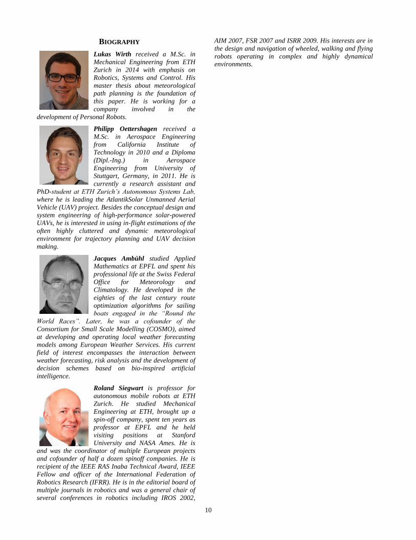
Lukas Wirth received a M.Sc. in
Mechanical Engineering from ETH
Zurich in 2014 with emphasis on
Robotics, Systems and Control. His
master thesis about meteorological
path planning is the foundation of
this paper. He is working for a
company involved in the
development of Personal Robots.
Philipp Oettershagen received a
M.Sc. in Aerospace Engineering
from California Institute of
Technology in 2010 and a Diploma
(Dipl.-Ing.) in Aerospace
Engineering from University of
Stuttgart, Germany, in 2011. He is
currently a research assistant and
PhD-student at ETH Zurich’s Autonomous Systems Lab,
where he is leading the AtlantikSolar Unmanned Aerial
Vehicle (UAV) project. Besides the conceptual design and
system engineering of high-performance solar-powered
UAVs, he is interested in using in-flight estimations of the
often highly cluttered and dynamic meteorological
environment for trajectory planning and UAV decision
making.
Jacques Ambühl studied Applied
Mathematics at EPFL and spent his
professional life at the Swiss Federal
Office for Meteorology and
Climatology. He developed in the
eighties of the last century route
optimization algorithms for sailing
boats engaged in the “Round the
World Races”. Later, he was a cofounder of the
Consortium for Small Scale Modelling (COSMO), aimed
at developing and operating local weather forecasting
models among European Weather Services. His current
field of interest encompasses the interaction between
weather forecasting, risk analysis and the development of
decision schemes based on bio-inspired artificial
intelligence.
Roland Siegwart is professor for
autonomous mobile robots at ETH
Zurich. He studied Mechanical
Engineering at ETH, brought up a
spin-off company, spent ten years as
professor at EPFL and he held
visiting positions at Stanford
University and NASA Ames. He is
and was the coordinator of multiple European projects
and cofounder of half a dozen spinoff companies. He is
recipient of the IEEE RAS Inaba Technical Award, IEEE
Fellow and officer of the International Federation of
Robotics Research (IFRR). He is in the editorial board of
multiple journals in robotics and was a general chair of
several conferences in robotics including IROS 2002,
AIM 2007, FSR 2007 and ISRR 2009. His interests are in
the design and navigation of wheeled, walking and flying
robots operating in complex and highly dynamical
environments.
11
APPENDIX A
Additional validation case with unsuitable weather conditions
20 m
s
60 50 40 30 20 10
30
40
50
60
Total cloud cover on Wed 5 Jun 2013 06:00:00UTC
Flight time: 24h UTC: Wed 5 Jun 2013 06:00:00 Local time: Wed 5 Jun 2013 03:37:05
20 m
s
60 50 40 30 20 10
30
40
50
60
Total cloud cover on Tue 4 Jun 2013 18:00:00UTC
Flight time: 12h UTC: Tue 4 Jun 2013 18:00:00 Local time: Tue 4 Jun 2013 15:16:29
30
40
50
60°N
-10-20-30-40-50 °E-60
20 𝑚𝑠
Flight time 12h – Tue 4 Jun 2013 18:00:00 UTC
20 m
s
60 50 40 30 20 10
30
40
50
60
Total cloud cover on Thu 6 Jun 2013 06:00:00UTC
Flight time: 48h UTC: Thu 6 Jun 2013 06:00:00 Local time: Thu 6 Jun 2013 04:12:44
20 m
s
60 50 40 30 20 10
30
40
50
60
Total cloud cover on Fri 7 Jun 2013 06:00:00UTC
Flight time: 72h UTC: Fri 7 Jun 2013 06:00:00 Local time: Fri 7 Jun 2013 04:51:59
30
40
50
60°N
-10-20-30-40-50 °E-60
20 𝑚𝑠
Flight time 24h – Wed 5 Jun 2013 06:00:00 UTC
30
40
50
60°N
-10-20-30-40-50 °E-60
20 𝑚𝑠
Flight time 48h – Thu 6 Jun 2013 06:00:00 UTC
30
40
50
60°N
-10-20-30-40-50 °E-60
20 𝑚𝑠
Flight time 72h – Fri 7 Jun 2013 06:00:00 UTC
threshold
limit
0 20 40 60 80h0
20
40
60
80
100
Relative humidity
0 20 40 60 80h
500
1000
1500
m
Altitude above sealevel
0 20 40 60 80
h0
5
10
15
20
25
30
m
s
Flight speed
airspeed groundspeed
0 20 40 60 80
h0
5000
10 000
15 000
_
Accumulated general cost
time SoC power cons . rad . factor environmental
0 20 40 60 80
h0
200
400
600
800
1000
W
m2
Global radiation on horizontal surface
total direct clear sky
100
80
60
40
20
% State of Charge Global Radiation on Horizontal Surface Accumulated Costs
threshold
limit
0 20 40 60 80 h
2000
1500
1000
500
0
[-]
SoCPower Consumption
TimeEnvironment
Radiation
800
600
400
200
0
𝑚2
Total Direct Clear-sky0 20 40 60 80 h 0 20 40 60 80 h
Relative Humidity
0 20 40 60 80 h
100
60
40
20
0
%
0 20 40 60 80 h 0 20 40 60 80 h
Altitude above MSLFlight Speed
Ground Speed Airspeed
m
1500
1000
500
15
10
25
𝑚
0
5
20
limit
threshold80
Figure 13 – The validation case with unsuitable weather conditions shows a path that starts with heavy winds and
high cloud coverage. In the first night, the SoC is critically low. The airspeed needs to be increased temporarily to
maintain a certain ground speed. Costs for SoC, power consumption, radiation and environmental dangers cannot be
totally avoided.