Meteor Trail Echo Rejection in Atmospheric Phased …tsato/publ-pdf/jtech2014.pdfMeteor Trail Echo...
9
Meteor Trail Echo Rejection in Atmospheric Phased Array Radars Using Adaptive Sidelobe Cancellation TAISHI HASHIMOTO Department of Communications and Computer Engineering, Kyoto University, Kyoto, Japan KOJI NISHIMURA AND MASAKI TSUTSUMI National Institute of Polar Research, Tachikawa, Japan TORU SATO Department of Communications and Computer Engineering, Kyoto University, Kyoto, Japan (Manuscript received 6 February 2014, in final form 21 May 2014) ABSTRACT Strong meteor trail echoes are interferences in the wind velocity estimates made from mesosphere radar observations. Contaminated spectra are detected by their discontinuity and are removed at the risk of greater fluctuations of spectra, leading to a severe reduction of the signal-to-noise ratio (SNR) and inaccurate wind estimates for weak atmospheric echoes. This paper presents an adaptive signal processing technique for the suppression of spectral contaminations by meteor trail echoes. The method is based on the norm-constrained and directionally constrained minimization of power (NC-DCMP), which balances the capability of canceling the clutter and the robustness of beam shaping, at the cost of a slight decrease in the SNR, which can be determined in advance. Simulation results show that with a 3-dB decrease of the SNR being allowed, the method improves the signal-to-interference ratio (SIR) by 15 dB, giving wind estimates that are about 8 m s 21 better in terms of root-mean-square error and providing 4 times as wide an observable range when compared with the results of the ordinary nonadaptive beamforming method. The results for an actual observation show that the improvement of both the SIR and the observable range are achieved as in the simulations, which implies that the method should provide the simulated accuracy for the estimation of wind velocity from actual observations. 1. Introduction In observations of mesosphere wind employing Doppler radars, strong meteor echoes often contaminate spectra. Usually, these spectra with meteor echoes are automati- cally detected by their discontinuity in time and height, and are discarded before the incoherent integration and wind velocity estimation are made (Tsuda et al. 1985). How- ever, only outstanding echoes can be removed employ- ing this method. Additionally, decreasing the number of spectra for incoherent integration increases the fluctu- ations of spectra, which introduces estimation errors of the wind velocity of weak mesosphere echoes. This paper presents an adaptive signal processing technique for reducing interferences from meteor trail echoes in mesosphere wind observations. The base method has been shown to be a good solution for the rejection of interference from the ground (Kamio et al. 2004) and ac- curate estimation of the vertical wind velocity (Nishimura et al. 2012). However, this is not the case for rapidly moving objects such as aircraft. Meteor trail echoes are also moving objects and have strong echo intensity, but they are relatively slow and the method works well for them. The contents of this paper are as follows. In section 2, the theory and implementation of the method are stated. Section 3 explains the simulation model and gives the result of applying the adaptive meteor clutter rejec- tion technique to the model. In section 4, we apply the Denotes Open Access content. Corresponding author address: Taishi Hashimoto, Dept. of Communications and Computer Engineering, Kyoto University, Yoshida-Hommachi, Sakyo-ku, Kyoto 606-8501, Japan. E-mail: [email protected] DECEMBER 2014 HASHIMOTO ET AL. 2749 DOI: 10.1175/JTECH-D-14-00035.1 Ó 2014 American Meteorological Society
Transcript of Meteor Trail Echo Rejection in Atmospheric Phased …tsato/publ-pdf/jtech2014.pdfMeteor Trail Echo...

Meteor Trail Echo Rejection in Atmospheric Phased Array Radars UsingAdaptive Sidelobe Cancellation
TAISHI HASHIMOTO
Department of Communications and Computer Engineering, Kyoto University, Kyoto, Japan
KOJI NISHIMURA AND MASAKI TSUTSUMI
National Institute of Polar Research, Tachikawa, Japan
TORU SATO
Department of Communications and Computer Engineering, Kyoto University, Kyoto, Japan
(Manuscript received 6 February 2014, in final form 21 May 2014)
ABSTRACT
Strong meteor trail echoes are interferences in the wind velocity estimates made from mesosphere radar
observations. Contaminated spectra are detected by their discontinuity and are removed at the risk of greater
fluctuations of spectra, leading to a severe reduction of the signal-to-noise ratio (SNR) and inaccurate wind
estimates for weak atmospheric echoes. This paper presents an adaptive signal processing technique for the
suppression of spectral contaminations by meteor trail echoes. The method is based on the norm-constrained
and directionally constrained minimization of power (NC-DCMP), which balances the capability of canceling
the clutter and the robustness of beam shaping, at the cost of a slight decrease in the SNR, which can be
determined in advance. Simulation results show thatwith a 3-dBdecrease of the SNRbeing allowed, themethod
improves the signal-to-interference ratio (SIR) by 15dB, giving wind estimates that are about 8ms21 better in
terms of root-mean-square error and providing 4 times as wide an observable range when compared with the
results of the ordinary nonadaptive beamforming method. The results for an actual observation show that the
improvement of both the SIR and the observable range are achieved as in the simulations, which implies that
the method should provide the simulated accuracy for the estimation of wind velocity from actual observations.
1. Introduction
In observations ofmesospherewind employingDoppler
radars, strong meteor echoes often contaminate spectra.
Usually, these spectra with meteor echoes are automati-
cally detected by their discontinuity in time andheight, and
are discarded before the incoherent integration and wind
velocity estimation are made (Tsuda et al. 1985). How-
ever, only outstanding echoes can be removed employ-
ing this method. Additionally, decreasing the number of
spectra for incoherent integration increases the fluctu-
ations of spectra, which introduces estimation errors of
the wind velocity of weak mesosphere echoes.
This paper presents an adaptive signal processing
technique for reducing interferences from meteor trail
echoes inmesospherewindobservations. The basemethod
has been shown to be a good solution for the rejection of
interference from the ground (Kamio et al. 2004) and ac-
curate estimation of the vertical wind velocity (Nishimura
et al. 2012).However, this is not the case for rapidlymoving
objects such as aircraft. Meteor trail echoes are also
moving objects and have strong echo intensity, but they
are relatively slow and the method works well for them.
The contents of this paper are as follows. In section 2,
the theory and implementation of themethod are stated.
Section 3 explains the simulation model and gives the
result of applying the adaptive meteor clutter rejec-
tion technique to the model. In section 4, we apply the
Denotes Open Access content.
Corresponding author address: Taishi Hashimoto, Dept. of
Communications and Computer Engineering, Kyoto University,
Yoshida-Hommachi, Sakyo-ku, Kyoto 606-8501, Japan.
E-mail: [email protected]
DECEMBER 2014 HASH IMOTO ET AL . 2749
DOI: 10.1175/JTECH-D-14-00035.1
� 2014 American Meteorological Society

method to an actual observation and show the result.
Section 5 summarizes the proposed method and gives
conclusions.
2. Methods and implementations
In this section, adaptive signal processing methods
and their implementations are stated.
a. Directionally constrained minimization of power
The directionally constrained minimization of power
(DCMP) algorithm is an adaptive beamforming algo-
rithm for the special case of known desired directions.
According to Takao et al. (1976), the basic theory of
DCMP is written as a nonlinear optimization problem:
Wmin�Pout 5
1
2WHRxxW
�subject to CTW*5H , (1)
where (�)* denotes the complex conjugate, (�)T is for the
transposition, and (�)H is for the adjoint (conjugate
transpose) matrix. AssumingM receivers, Rxx [XXH is
the covariancematrix of the received signalsX5 [X1, . . . ,
XM]T andW is the optimalweight vector. TermC is called
the directional constraint, which is a function of the
geometric location of each receiver Li (i5 1, . . . ,M) and
the desired direction (zenith, azimuth)5 (u, f). Using an
array manifold function A(u, f), Ci can be written as
Ci 5Ai(u,f)5 exp
�2pi
lLi �V
�
V5 [sinu cosf, sinu sinf, cosu]T . (2)
Term l is the radar wavelength and H is called the
constraint response against each corresponding C; H
takes a value from 0 to 1 and determines the null depth
or the peak height of the beam pattern in the specific
direction defined by C. Term V is a unit vector to the
radial direction (u, f). The combined outputs of beam
synthesis Y is obtained by
Y5WHX . (3)
b. Norm-constrained DCMP
The norm-constrained DCMP (NC-DCMP) has an
additional constraint of the magnitude of the norm of
W in Eq. (1):
WHW#U . (4)
Here, U is the norm constraint that preserves the shape
of the main lobe even when only an incorrect steering
vector is available.
For the NC-DCMP algorithm, one can determine
U from the permissive loss in the signal-to-noise ratio
(SNR). The relationship between the SNR loss GSNR
and the norm constraint U is described in Kamio et al.
(2004):
GSNR5[11a
ffiffiffiffiffiffiffiffiffiffiffiffiffiffiffiffiffiffiffiffiffiffiU/(M2 1)
p]2
11U, (5)
where a takes a value from 21 to 1 and represents the
phase rotational relation between each channel. Equa-
tion a5 1 means an in-phase relation, which is obtained
employing the ideal beamforming method without
availability of clutter rejection. Equation a521 means
an opposite-phase relation, which is the worst case,
suppressing the desired signals. Equation a 5 0 is the
intermediate of these two cases and is used to decide the
norm constraint U in later sections. Figure 1 is an ex-
ample of plotting Eq. (5) at each a521, 0, 1 forM5 25,
which corresponds to the number of channels of the
middle and upper (MU) atmosphere radar.
c. Norm-constrained tamed adaptive antenna
As mentioned above, NC-DCMP requires the solving
of a nonlinear optimization problem with an inequality
constraint, which severely increases the calculation cost.
However, according to Wang et al. (2003), the norm
WHW is known to decreasemonotonically as b increases
and in the special case of the equality of Eq. (4) being
satisfied, the solution can be easily obtained as
FIG. 1. Relationship between U and GSNR in the 25-channel ra-
dar system assuming the MU radar. The abscissa is U and the or-
dinate isGSNR. Each line corresponds to a different phase rotation:
a5 1 (in phase; top line),a521 (opposite phase; bottom line) and
a 5 0 (intermediate; middle line). We use the middle line for de-
ciding U.
2750 JOURNAL OF ATMOSPHER IC AND OCEAN IC TECHNOLOGY VOLUME 31

W5R21xx C
CHR21xx C
H*,
Rxx[Rxx 1bI , (6)
where I is a unit matrix and b . 0 represents the mag-
nitude of the pseudonoise added to the covariancematrix.
The solution in Eq. (6) is exactly the same as the optimal
weight vector of the tamed adaptive antenna array men-
tioned in Takao and Kikuma (1986), but b cannot be
obtained directly. Thus, b is determined as follows:
(i) Estimate the boundary of the norm constraint U
from the permissive SNR loss GSNR using Eq. (5).
(ii) Set b 5 0 and calculate Wb50. If Eq. (4) is already
satisfied by Wb50, then this solution is optimal.
Otherwise, continue to the next.
(iii) Find the minimum b that satisfies the equality
condition of Eq. (4). This can be effectively calcu-
lated employing a one-dimensional root-finding
algorithm such as Newton’s method.
We call this method, which is an effective way to cal-
culate the optimal weight of NC-DCMP, the norm-
constrained tamed adaptive (NC-TA) method in later
sections. Depending on the selection of U, the NC-TA
method may fail in finding the optimal weight vectorW.
Thus, in practice, one can start this routine with small U
and then iterate by increasing GSNR.
3. Simulation of adaptive meteor clutter rejection
In this section, we show the result of simulations of the
adaptive meteor clutter rejection technique for meso-
spheric radar observations.
a. Generating simulation data of atmospheric andmeteor echoes
In this simulation, each spectrum contains two kinds
of echoes, atmospheric and meteor echoes. In the fol-
lowing subsections, detailed procedures of generating
atmospheric and meteor echoes are stated.
1) ATMOSPHERIC ECHOES
Power spectra of atmospheric echoes returned by
backscattering from turbulences are modeled by a
Gaussian function as follows (Yamamoto et al. 1988):
Sm(y)5PSffiffiffiffiffiffi2p
psexp
"2(y2 yd)
2
2s2
#1PN , (7)
where y is the radial wind velocity, PS is the echo in-
tensity of the atmospheric echo, PN is the noise floor
level, yd is the mean Doppler velocity of the wind, and s
is the spectral width. Additionally, the time series of
complex outputs at each receiver has random fluctua-
tions following a Gaussian distribution for both real and
imaginary components. This results in the model spec-
trum having the statistical fluctuation following a x2
distribution with 2 degrees of freedom, because the
power spectra are the squared sum of complex received
signals. The model spectrum with these fluctuations,
S0m(y), can now be obtained as the product of Sm(y) and
random numbers following a x2 distribution with 2 de-
grees of freedom.
For the adaptive signal processing, we need complex
outputs at each receiver si(t) (i 5 1, . . . , M , where M is
the number of receivers). To reproduce these from
S0m(y), we can use the inverse Fourier transform and the
array manifold, which is stated in the previous section.
First, we perform the inverse Fourier transform to ob-
tain the basic complex outputs at the phase origin, so(t),
which is a time series:
so(t)5F21[ffiffiffiffiffiffiffiffiffiffiffiffiS0m(y)
q: r(y)] , (8)
where A:B represents a complex number with its
amplitude A and phase B, F21[�] stands for the inverse
Fourier transform, and r(y) is a uniform random-
number generator having a range of [0, 2p]. As shown
by Eq. (8), amplitudes are set to the square root of S0m(y)and phases are assumed to be uniform random variables
in the range of [0, 2p]. A time series at each receiver sican then be calculated by rotating phases of so(t) by
using the array manifold Eq. (2),
si(t)5Ai(u,f)so(t) , (9)
where (u, f) is the desired direction of the radar system.
2) METEOR ECHOES
Meteor trail echoes are returned from ionized elec-
trons left along the paths of meteoroids. These trails
usually remain at most a second with 50MHz and pro-
vide strong backscattering. For example, the echo power
from these trails may reach 80 dB over the noise level
(McKinley 1961). In radar observations of the meso-
sphere, successive spectra are usually averaged to reduce
statistical fluctuations. This procedure is called in-
coherent integration. Although these meteor trails fade
out in less than a second, their strong intensity contami-
nates the spectra severely even after the incoherent
integration.
In this simulation, a meteor trail echo is modeled as
a backscattering from a linearly shaped hard target with
exponentially decreasing echo power that is moved by
the background wind; that is, underdense meteor trail.
DECEMBER 2014 HASH IMOTO ET AL . 2751

Phases of the meteor echo pi(t) can be calculated from
the distance to each receiver di(t). Amplitudes are the
square root of the meteor echo power PM(t), which is
known to decay exponentially as
PM(t)5PM(0) exp
�232p2Dt
l2
�, (10)
whereD is the ambipolar diffusion coefficient (Ceplecha
et al. 1998). We use D ; 1m2 s21 at 90 km. Conse-
quently, the time series ofmeteor trail echoes si(t) can be
obtained as
si 5PM(t) expipi(t) . (11)
3) SIGNAL PROCESSING
After generating received signals for both atmo-
spheric and meteor echoes, we add them together and
obtain the complex time series
s(t)5 [s1(t), s2(t), . . . , sM(t)]T (12)
for each channel. The covariance matrix Rxx for sample
number kt is generated and updated using the following
set of expressions:
Rxx(0)5 s(0)sH(0),
Rxx(kt)5 gRxx(kt 2 1)1 (12 g)s(kt)sH(kt) , (13)
where kt5 1, 2, . . . and 0# g, 1 is the forgetting factor.
In this simulation, we use g 5 0.995, which is the
equivalent of accumulating received signals of about
1500 samples to obtain one covariance matrix. The time
series of received signals s(t) is synthesized employing
twomethods to make a comparison, the NC-TAmethod
and nonadaptive beamforming (NA-BF) method. For
each renewal of the covariance matrix, an optimal
weight vector W(t) is calculated using Eq. (6) for the
NC-TAmethod, with a5 0 andM5 25. The permissive
SNR loss GSNR is set as an increasing sequence of five
equal intervals in the range from 0.5 to 3 dB. For the
NA-BF method, W(t) 5 A(u, f) using an array mani-
fold. The desired direction (u, f) is set to (08, 08). Thebeam synthesis of the received signals using the weight
vector W is performed through Eq. (3).
4) INCOHERENT INTEGRATION
After the beam synthesis of the received signals and
calculation of spectra, we perform incoherent integra-
tion by accumulating Ni successive spectra. The fluctu-
ation of amplitudes is expected to be reduced to 1/ffiffiffiffiffiNi
pin this manner. In practice, spectra with strong meteor
clutters should be removed from the integration. We set
a threshold Bt as 13.5 dB over the peak power of at-
mospheric echoPS for deciding which spectrum contains
a clutter and should be discarded. In this simulation, the
peak power of an atmospheric echo is known—for ex-
ample, 110 dB over the noise level. The probability of
random fluctuations being at least 13.5 dB over the ac-
tual peak power—for example,113.5 dB over the noise
level in this case—is less than 5% in the x2 distribution
with 2 degrees of freedom. Any peak over Bt is thus
assumed to be a clutter.
b. Wind velocity estimation employing the leastsquares fitting method
After the incoherent integration, we estimate the
mean wind velocities yd from the averaged spectra em-
ploying the least squares fitting method (Yamamoto
et al. 1988). This method fits a Gaussian spectrum
S(kn;PS, yd, s) to the simulated observed spectrum
S0m(kn), such that the root-mean-square (RMS) of the
residue
�5
ffiffiffiffiffiffiffiffiffiffiffiffiffiffiffiffiffiffiffiffiffiffiffiffiffiffiffiffiffiffiffiffiffiffiffiffiffiffiffiffiffiffiffiffiffiffiffiffiffiffiffiffiffiffiffiffiffiffiffiffiffiffiffiffiffiffiffiffiffiffiffiffiffiffiffiffiffi1
kn�kn
[S(kn;PS, yd,s)2S0m(kn)2PN]2
s(14)
isminimized by changing parametersPS, yd, ands. Here,
kn is the discrete sample number of frequency compo-
nents. Note that the noise level of the observed spec-
trum PN must be obtained in advance employing other
methods (Hildebrand and Sekhon 1974;Woodman 1985).
c. Simulation settings
1) RADAR SYSTEM
The target radar system is based on the MU radar at
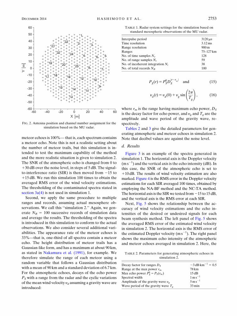
Shigaraki MU Observatory, Japan. Figure 2 shows the
antenna position and the group number of the MU ra-
dar. The MU radar has 475 crossed Yagi antennas and
the signals received from each of the 19 receivers are
combined into one channel, forming an adaptive antenna
with 25 channels. The radar frequency is 46.5MHz. Ob-
servational parameters are listed in Table 1. Note that
using Ni 5 38 successive spectra for incoherent in-
tegration is equivalent to averaging over about 1min.
2) EXPERIMENTAL PARAMETERS
We conduct two types of simulations. First, assuming
an arbitrary range with both atmospheric and meteor
echoes observed, we vary the SNR of the atmospheric
echoes and calculate the RMS error of the wind velocity
estimation at each SNR. We call this ‘‘simulation 1.’’ In
this simulation, we set themeteor clutter to have an echo
intensity of 115 dB over the noise level and consider
a radial velocity of 15m s21. The appearance rate of
2752 JOURNAL OF ATMOSPHER IC AND OCEAN IC TECHNOLOGY VOLUME 31
meteor echoes is 100%— that is, each spectrum contains
a meteor echo. Note this is not a realistic setting about
the number of meteor trails, but this simulation is in-
tended to test the maximum capability of the method
and the more realistic situation is given to simulation 2.
The SNR of the atmospheric echo is changed from 0 to
130 dB over the noise level, in steps of 5 dB. The signal-
to-interference ratio (SIR) is then moved from 215 to
115 dB. We run this simulation 100 times to obtain the
averaged RMS error of the wind velocity estimations.
The thresholding of the contaminated spectra stated in
section 3a(4) is not used in simulation 1.
Second, we apply the same procedure to multiple
ranges and records, assuming actual mesosphere ob-
servations. We call this ‘‘simulation 2.’’ Again, we gen-
erate NR 5 100 successive records of simulation data
and average the results. The thresholding of the spectra
is introduced in this simulation to conform to the actual
observations. We also consider several additional vari-
abilities. The appearance rate of the meteor echoes is
33%—that is, one-third of all spectra contain a meteor
echo. The height distribution of meteor trails has a
Gaussian-like form, and has a maximum at about 90 km,
as stated in Nakamura et al. (1991), for example. We
therefore simulate the range of each meteor using a
random variable that follows a Gaussian distribution
with amean of 90 km and a standard deviation of 6.7 km.
For the atmospheric echoes, decays of the echo power
PS with a range from the radar and the cyclic variations
of themeanwind velocity yd assuming a gravity wave are
introduced:
PS(r)5P0SD
jr2rmj
S and (15)
yd(t)5 yd(0)1 yg sin
2p
Tg
!, (16)
where rm is the range having maximum echo power, DS
is the decay factor for echo power, and yg and Tg are the
amplitude and wave period of the gravity wave, re-
spectively.
Tables 2 and 3 give the detailed parameters for gen-
erating atmospheric and meteor echoes in simulation 2.
Note that decibel values are against the noise level.
d. Results
Figure 3 is an example of the spectra generated in
simulation 1. The horizontal axis is the Doppler velocity
(m s21) and the vertical axis is the echo intensity (dB). In
this case, the SNR of the atmospheric echo is set to
110dB. The results of wind velocity estimation are also
marked. Figure 4 is the RMS error in the Doppler velocity
estimations for each SIR averaged 100 times, obtained by
employing the NA-BF method and the NC-TA method.
Thehorizontal axis is the SIRwe tested from215 to 15dB,
and the vertical axis is the RMS error at each SIR.
Next, Fig. 5 shows the relationship between the ac-
curacy of wind velocity estimations and the echo in-
tensities of the desired or undesired signals for each
beam synthesis method. The left panel of Fig. 5 shows
the averaged RMS error of the estimated wind velocity
in simulation 2. The horizontal axis is the RMS error of
the estimated Doppler velocity (m s21). The right panel
shows the maximum echo intensity of the atmospheric
and meteor echoes averaged in simulation 2. Here, the
TABLE 1. Radar system settings for the simulation based on
standard mesospheric observations of the MU radar.
Interpulse period 3120ms
Time resolution 3.12ms
Range resolution 900m
Ranges 75–127 km
No. of time samples Nn 128
No. of range samples Nr 59
No. of incoherent integration Ni 38
No. of total records NR 100
TABLE 2. Parameters for generating atmospheric echoes in
simulation 2.
Decay factor for ranges DS 23 dBkm21 5 0.5
Range at the max power rm 78 km
Max echo power P0S 5PS(rm) 15 dB
Spectral width 1m s21
Amplitude of the gravity wave yg 5m s21
Wave period of the gravity wave Tg 33min
FIG. 2. Antenna position and channel number assignment for the
simulation based on the MU radar.
DECEMBER 2014 HASH IMOTO ET AL . 2753

atmospheric echo has a peak power around 78 km, while
the intensity of meteor echoes increases with range. The
vertical axes of the two panels have units of kilometers.
e. Discussion
In simulation 1, all spectra are used without thresh-
olding. In such a case, the adaptive meteor clutter re-
jection technique is found to improve the accuracy of the
wind velocity estimations, especially when the inter-
ference is stronger than or almost equal to the atmo-
spheric echoes. As seen in Fig. 3, the meteor clutter is
suppressed well by the NC-TA method. Thus, wind ve-
locities are estimated near the true peak by the NC-TA
method, while the NA-BF method gives wrong values
contaminated by meteor clutters. Consequently, Fig. 4
shows that with SIRs under 0 dB, as in Fig. 3, the echo
intensity of meteor clutters is stronger than that of at-
mospheric echoes and theNA-BFmethod gives incorrect
estimations of wind velocity because of the interference.
As a result, the observable echo intensity improves by
about 15 dB when employing the NC-TA method. In
addition, we should mention that meteor trail echoes can
be extracted by employing the samemethod if needed, by
simply subtracting the obtained meteor-suppressed sig-
nals from the original received ones.
In simulation 2, strong interference is suppressed by
spectral thresholding. Employing this procedure, the
initial guess of the peak search is made accurate to some
extent by discarding contaminated spectra in incoherent
integration, while fewer spectra result in more fluctua-
tion in the integrated spectra, which can bring low ac-
curacy. Additionally, interferences below the threshold
remain with no changewith theNA-BFmethod, and this
leads to an increase in the RMS error in the spectral
fitting for the NA-BF method. On the contrary, the NC-
TA method suppresses interferences automatically in
advance, and improves both the number of spectra dis-
carded in incoherent integration and the RMS error in
the spectral fitting. These trends are clearly shown in
Fig. 5. Here, the NC-TA method discards only 1.3% of
spectra, while 10.9% with the NA-BF method. The av-
erage RMS errors at 78 km are 1.5m s21 for the NC-TA
method and 10.1m s21 for the NA-BF method. As seen
in Fig. 5b, the average SIR of simulation 2 is at most
210 dB at 78 km. Figure 4 shows that even the NC-TA
method gives low accuracy with the SIR under 210 dB
and thus the result is consistent with simulation 1. At
higher ranges, where there are more meteor echoes, the
accuracy of the estimated wind velocity is low for both
methods, but the error is about 8m s21 less for the NC-
TAmethod. Additionally, the RMS error has a flat floor
from 76 to 78 km with the NC-TA method, which is
about 4 times as wide as that with the NA-BF method.
This is the benefit of the adaptive clutter rejection
FIG. 3. Example of the spectra generated in simulation 1. The
SNR of the atmospheric echo is 110 dB. Lines are the spectra of
the atmosphere only, meteor only, and the synthesized spectra of
the NA-BF method and the NC-TA method. Marks show the ac-
tual peak powers and Doppler velocities and the peak powers and
Doppler velocities estimated employing the NA-BF method and
the NC-TA method.
FIG. 4. RMS error of wind velocity estimated with the NA-BF
method and the NC-TAmethod. The horizontal axis is the SIR and
the vertical axis is the RMS error between the true velocity and the
estimated velocity.
TABLE 3. Parameters for generating meteor echoes in simulation 2.
Mean of power distribution P0 20 dB
Std dev of power distribution sP 2.5 dB
Mean of range distribution 90 km
Std dev of range distribution 6.7 km
Appearance rate 33%
Radial velocity 0–25m s21
Diffusion coefficient D 1.0m2 s21
Orientation Uniformly random
2754 JOURNAL OF ATMOSPHER IC AND OCEAN IC TECHNOLOGY VOLUME 31

technique and implies the effectiveness of the technique
in mesosphere observations.
4. Applying the adaptive meteor clutter rejectiontechnique to an actual observation
This section presents results of applying the adaptive
meteor clutter rejection technique to actual mesospheric
observations.
a. Observational settings of the radar system
A series of meteor observations was made on 8 Oc-
tober 2011 at Shigaraki MU Observatory. We use NR 5100 successive records taken from 1405 to 1546 UTC.
The observational parameters are listed in Table 4. As
done in simulation 2 of section 3, the time resolution of
the adaptive beam synthesis is 3.12ms. After the clutter
cancellation, Ni 5 38 successive spectra are used for
incoherent integration to obtain each record, which is
equivalent to averaging over about 1min.
b. Signal processing
We apply the NA-BFmethod and the NC-TAmethod
to the same observed data sequence to compare the
ability of the two methods to suppress clutter. Pro-
cedures of the signal processing are exactly the same as
those described in section 3. Additionally, thresholding
and accumulation of spectra are performed as in the
previous section. However, the threshold Bt for re-
moving contaminated spectra is unknown for the actual
observation, and we determine it as follows. First, we
perform adaptive beam synthesis on all received sig-
nals, employing the NA-BF method and the NC-TA
method, and then convert them into spectra by taking
the Fourier transform to obtain synthesized spectra
S(kT, kn), where kT 5 1, . . . , Ni 3NR is the spectrum
index and kn 5 1, . . . , Nn is the frequency component
index.We then take the frequency-wise sumof S(kT, kn) as
S(kT)5 �N
n
kn51
S(kT ,kn) . (17)
FIG. 5. (a) RMS errors of the wind velocity estimations of the NA-BFmethod and the NC-TAmethod. The ordinate
has a unit of kilometers. (b) Intensities of the atmospheric and meteor echoes for each range.
TABLE 4. Radar system settings for the observation made by the
MU radar from 1405 to 1546 UTC 8 Oct 2011.
Interpulse period 3120ms
Time resolution 3.12ms
Range resolution 900m
Valid ranges 75–127 km
No. of time samples Nn 512
No. of range samples Nr 59
No. of incoherent integration Ni 38
No. of total records NR 100
DECEMBER 2014 HASH IMOTO ET AL . 2755

Finally, we choose the thresholdBt to satisfy the relation
p[S(kT).Bt]# 5% (18)
at ranges of 74–80 km. Here, p[S(kT).Bt] is the prob-
ability of peaks in S(kT) being larger than the current
threshold Bt. The objective of Eq. (18) is to make the
number of discarded spectra the same as in the simula-
tion of the previous section. To compute Bt, we itera-
tively enlarge Bt to find the minimum value that satisfies
Eq. (18). The overlaid spectral peaks are shown in Figs. 6
and 7 for the NA-BF method and the NC-TA methods,
respectively. The horizontal axis is the peak power for
each range (dB) and the vertical axis is the range (km).
Dashed lines are the threshold Bt for the spectra pro-
cessed by the two methods.
c. Results
Table 5 gives the threshold Bt we selected for re-
moving spectra with contaminations, the defection ratio
FD in the incoherent integration, and the equivalent
number of incoherent integration h. Figure 8 shows the
average errors of the wind velocity estimation versus
the range (74–84 km) estimated from spectra processed
with the NA-BF method and the NC-TA method. Thin
lines are biased by the standard deviation s for each
range.
d. Discussion
1) COMPARISON OF THE DEFECTION RATIO
Table 5 shows that the NC-TA method discards only
about one-third of the spectra discarded by the NA-BF
method through thresholding in incoherent integration.
Additionally, comparing Figs. 6 and 7, it is clear that the
number of peaks in spectra processed by the NC-TA
method that are considered to be meteor clutters is
much less than that in the case of the NA-BF method.
The average suppression ratio of meteor clutters is
nearly 15 dB, which is the same result as for simulation 1
in section 3.
2) DIFFERENCES IN WIND VELOCITY ESTIMATION
As seen in Fig. 8, the standard deviations of the av-
erage wind velocities at ranges of 78–80 km and 73.7 km
estimated with the NC-TAmethod are much lower than
those estimated with the NA-BF method. These ranges
are considered to be the boundary regions where at-
mospheric echoes are weak and meteor clutters are
dominant. However, the NC-TAmethod works for both
clutter suppression and decreasing fluctuations of spec-
tra and these benefits lead to observable ranges that are
almost twice as wide.
5. Summary and conclusions
This paper presented the result of applying an adap-
tive meteor clutter rejection technique to an actual
mesosphere observation.
FIG. 6. Peaks of spectra processed by the NA-BF method for
each range overlaid throughout the observation period on 8 Oct
2011. The horizontal axis is the peak power for each range (dB) and
the vertical axis is the range (km). The dashed line is the threshold
Bt we selected.
FIG. 7. As in Fig. 6, but processed with the NC-TA method.
TABLE 5. Threshold Bt for discarding contaminated spectra in
incoherent integration, the defection ratio FD with thresholding,
and the equivalent number of incoherent integration h for the
observation.
BF NC-TA
Bt 31.4 dB 28.6 dB
FD 13.5% 4.37%
h ’32.9 ’36.3
2756 JOURNAL OF ATMOSPHER IC AND OCEAN IC TECHNOLOGY VOLUME 31

In section 3, we presented the results from two simu-
lations. First, we examined the capability of the NC-TA
method to suppress contaminations. The NC-TA
method reproduced the desired signals with the SNRs
exceeding 15 dB (SIR of 25 dB), which is an improve-
ment of115 dB comparedwith the result of the ordinary
nonadaptive beamforming method. Second, we per-
formed a more realistic simulation of a mesosphere
observation. In this case, the method estimates the wind
velocity with an RMS error of about 1.5m s21 with an
SIR of210 dB, and the spectral fitting was successful for
ranges 4 times as wide as in the case of the nonadaptive
beamforming method.
In section 4, the NC-TA method was applied to an
actual observation made on 8 October 2011. The pro-
posed method suppressed meteor clutters by about
15 dB on average, and the number of spectra discarded
through spectral thresholding in incoherent integration
with the NC-TA method was about one-third of the
number for the nonadaptive beamforming method.
Additionally, the standard deviation of the wind velocity
estimation was less than 2m s21 for ranges twice as wide
as those for the conventional method—that is, the ob-
servable range doubled.
The above-mentioned simulation and observational re-
sults show that the NC-TA method is a good solution for
mesosphere observations contaminated bymeteor clutters.
REFERENCES
Ceplecha, Z., J. Borovi�cka, W. G. Elford, D. O. ReVelle, R. L.
Hawkes, V. Porub�can, and M. �Simek, 1998: Meteor phenom-
ena and bodies. Space Sci. Rev., 84, 327–471, doi:10.1023/
A:1005069928850.
Hildebrand, P. H., and R. Sekhon, 1974: Objective determination
of the noise level inDoppler spectra. J.Appl.Meteor., 13, 808–811,
doi:10.1175/1520-0450(1974)013,0808:ODOTNL.2.0.CO;2.
Kamio, K., K. Nishimura, and T. Sato, 2004: Adaptive sidelobe
control for clutter rejection of atmospheric radars. Ann.
Geophys., 22, 4005–4012, doi:10.5194/angeo-22-4005-2004.
McKinley, D.W.R., 1961:Meteor Science andEngineering.McGraw-
Hill Series in Engineering Sciences, McGraw-Hill, 309 pp.
Nakamura, T., T. Tsuda, M. Tsutsumi, K. Kita, T. Uehara, S. Kato,
and S. Fukao, 1991: Meteor wind observations with the MU
radar. Radio Sci., 26, 857–869, doi:10.1029/91RS01164.
Nishimura, K., T. Nakamura, T. Sato, and K. Sato, 2012: Adap-
tive beamforming technique for accurate vertical wind mea-
surements with multichannel MST radar. J. Atmos. Oceanic
Technol., 29, 1769–1775, doi:10.1175/JTECH-D-11-00211.1.
Takao, K., and N. Kikuma, 1986: Tamed adaptive antenna array.
IEEE Trans. Antennas Propag., 34, 388–394, doi:10.1109/
TAP.1986.1143821.
——, M. Fujita, and T. Nishi, 1976: An adaptive antenna array
under directional constraint. IEEE Trans. Antennas Propag.,
24, 662–669, doi:10.1109/TAP.1976.1141411.
Tsuda, T., M. Yamamoto, T. Sato, S. Kato, and S. Fukao, 1985:
Comparison observations between the MU radar and the
Kyoto meteor radar. Radio Sci., 20, 1241–1246, doi:10.1029/
RS020i006p01241.
Wang, Z., J. Li, and P. Stoica, 2003: Comparison between norm
constrained and robust capon beamformers. IEEE In-
ternational Symposium on Phased Array Systems and Tech-
nology 2003, IEEE, 170–175.
Woodman, R. F., 1985: Spectral moment estimation inMST radars.
Radio Sci., 20, 1185–1195, doi:10.1029/RS020i006p01185.
Yamamoto, M., T. Sato, P. May, T. Tsuda, S. Fukao, and S. Kato,
1988: Estimation error of spectral parameters of mesosphere-
stratosphere-troposphere radars obtained by least squares
fitting method and its lower bound. Radio Sci., 23, 1013–1021,
doi:10.1029/RS023i006p01013.
FIG. 8. Average RMS errors in wind velocity estimation for each
range calculated with the NA-BFmethod and the NC-TAmethod.
Thin lines are biased by 61s.
DECEMBER 2014 HASH IMOTO ET AL . 2757