Metals and Alloys - Phase Transformations and Complex ... · AH1 Materials Science and Metallurgy,...

AH1 Materials Science and Metallurgy, 2nd year course H. K. D. H. Bhadeshia

Metals and Alloys

The development of improved metallic materials is a vital activity at the leading edge ofscience and technology. Metals offer unrivalled combinations of properties and reliability at acost which is affordable. They are versatile because subtle changes in their microstructure cancause dramatic variations in their properties. For example, it is possible to buy commercialsteel with a strength as low as 50 MPa or as high as 5500 MPa. An apple weighs about aNewton. The strongest commercial steel can therefore support the weight of about 5.5 × 109

apples on 1 m2 of steel. An understanding of the development of microstructure in metals isessential for the materials scientist. Thus, 70% of all 800 million tonnes per annum of alloysused today were developed in the last ten years.

Course A builds on the coverage of metals and alloys in Part IA. Whereas Part IA dealt withthe thermodynamics aspects, we shall emphasize kinetics when treating diffusion, solidificationand solid–state phenomena:

Diffusion

1. Fundamentals of Diffusion. Diffusive flux and the diffusion equation. Diffusion distances.Mechanisms of diffusion. Interstitial, substitutional and vacancy diffusion. Activation energiesand vacancy concentrations. Diffusivity data. Interdiffusion in alloys. Kirkendall effect.

2. Diffusion and Microstructure. Fast diffusion paths. Grain–boundary, free–surface and latticediffusion. Thermodynamics of diffusion. Chemical potential and atomic mobility. Ideal andnon–ideal solutions. Concept of zero, negative diffusivity and uphill diffusion.

Solidification

3. Undercooling and driving force. Nucleation and crystal growth. Heat flow. Solute partitioning.Effect of convection. The Scheil equation.

4. Solidification Structure. Constitutional undercooling, cells and dendrites. Microsegregationprofiles. Coring and non-equilibrium second phase. Grain structures, single crystals andpolycrystals.

5. Solidification Processing. Casting. Porosity and hot tearing. Sand casting. Permanent mouldcasting. Centrifugal casting. Continuous casting. Rapid solidification processing, atomisation,melt–spinning.

Solid–State Diffusional Transformations

6. Dislocations and Grain Boundaries. Cold–worked structures. Stored strain energies. Forcesbetween dislocations. Recovery processes, glide and climb. Polygonisation. Grain boundariesmisorientation, structure and energy.

7. Evolution of Grain Structure. Nucleation of recrystallised grains, role of dislocation density.Particle-stimulated nucleation. Mobility of high-angle grain boundaries. Solute drag and Zenerdrag. Grain growth.

8. Precipitation. Solution treatment, quenching and ageing. Precipitate nucleation. Precipitationsequences. Diffusion–controlled growth. Nucleation sites. Role of vacancies. Precipitate–freezones, solute and vacancy depletion.


Diffusionless Solid–State Transformations

9. Shear Transformations. Twinning, the twin plane and twinning shear. Twinning as a de-formation mode. Factors favouring deformation twinning. Strain–rate and crystal–symmetryeffects. Boundary energies. Martensitic transformations. Examples in cobalt and Fe–C. Theshape–memory effect.

Some Metallic Materials

10. Ferrous Alloys. The Fe–C phase diagram. The eutectoid reaction. Fe–C martensite. TTTcurves. Quenching and tempering of steels. Alloying effects and hardenability. The Jominyend–quench test. Widmanstatten ferrite and bainite. Secondary hardening in alloy steels.

11. TRIP steels. Dual–phase steels. Cast irons, grey, white and spheroidal graphitic. Light Alloys.Aluminium alloys. High-strength alloys.

12. High–Temperature Alloys. Nickel–based superalloys. Columnar and single–crystal turbineblades. Dispersion–strengthened alloys. Mechanically alloyed systems.

Aids to Learning

1. D. A. Porter and K. E Easterling, Phase Transformations in Metals and Alloys, 2nd editionChapman and Hall, (1992) [Ln30]

2. A. H. Cottrell, An Introduction to Metallurgy, The Institute of Materials, (1995) [A116]

3. R. W. K. Honeycombe and H. K. D. H. Bhadeshia, Steels, Microstructure and Properties, 2ndedition, Arnold, (1995) [De88]

4. I. J. Polmear, Light Alloys - Metallurgy of the Light Metals, 3rd edition, Arnold, (1995) [Eb153]

5. There are a number of metallographic samples associated with this course. They will be refer-enced in the question sheets. You will find it useful to examine these in the Class Laboratory.Be sure to handle these specimens carefully and to examine them at a variety of magnifications.Try and understand the microstructure in terms of the phase diagrams. A list of the samplesis included below; you will find relevant phase diagrams in your Data Book.

Code Composition / wt% Condition Etchant

M0 Fe-0.8C 1200 ◦C 2 h, furnace cooled nital

M7 Al-12Si as–cast in metal mould not etched

M8 Al–12Si–0.02Na as–cast in metal mould not etched

M24 Al–4Cu solution treated and over–aged NaOH


6. There is a Departmental Electronic Library which can be accessed on the world wide web.This contains useful additional material for this course. The material relevant to Course A islisted below, and there are regular additions to the contents:

On–line Teaching Library (Course A)

www.msm.cam.ac.uk/Department/Teaching/online.html

Lecture notes, question sheets & handouts

Worked Examples

Internet Supervisor

Microstructure of aluminium-copper alloys

Microstructure of aluminium-silicon alloys

Decarburization microstructures

Recrystallisation microstructures

Annealing twins

Precipitate-free zones

Dendritic solidification

Recrystallised grain size

Movies showing grain coarsening

Computer-generated movies of transformations

Actual movies of solidification


Fundamentals of Diffusion

The steady–state diffusive flux J is represented using Fick’s first law,

J = −D∂C∂x

where C is the concentration, x is a distance and D is the diffusion coefficient. Fick’s secondlaw is for cases where the concentration at any point varies with time t:

∂C

∂t= D

∂2C

∂x2

These equations can be solved for particular boundary conditions. For a case where a fixedquantity of solute is plated onto a semi–infinite bar (Fig. 1a),

boundary conditions:

∫ ∞

0

C{x, t}dx = B and C{x, t = 0} = 0

C{x, t} =B√πDt

exp

{−x2

4Dt

}

Now imagine that we create the diffusion couple illustrated in Fig. 1b, by stacking an infiniteset of thin sources on the end of one of the bars. Diffusion can thus be treated by taking awhole set of the exponential functions obtained above, each slightly displaced along the x axis,and summing (integrating) up their individual effects. The integral is in fact the error function

erf{x} =2√π

∫ x

0

exp{−u2}du

so the solution to the diffusion equation is

boundary conditions: C{x = 0, t}dx = Cs and C{x, t = 0} = C0

C{x, t} = Cs − (Cs − C0)erf

{x

2√Dt

}

Fig. 1: (a) Thin layer of solute plated on a semi–infinite bar. (b) Two different

semi–infinite bars.


Diffusivity Data

Most metals have similar diffusivities of about 10−12 m2 s−1 at their melting temperatures(Fig. 2). Silicon has the diamond cubic structure with directional bonding which makes theatoms less mobile in spite of the lower density associated with this crystal structure. Interstitialdiffusion is the fastest because of the free availability of interstitial vacancies. Thus, carbonhas about the same activation energy for diffusion as for the self–diffusion of aluminium, buta much larger diffusion coefficient at any temperature (Fig. 2).

Fig. 2: Typical self–diffusion coefficients for pure metals and for carbon

in ferritic iron. The uppermost diffusivity for each metal is at its melting

temperature.

TEMPERATURE

FREE

EN

ERG

Y

αγ

Transition Temperature


Thermodynamics of diffusion

Fick’s first law is empirical in that it assumes a proportionality between the diffusion flux andthe concentration gradient. However, diffusion occurs so as to minimise the free energy. Itshould therefore be driven by a gradient of free energy. But how do we represent the gradientin the free energy of a particular solute?

The Chemical Potential

We first examine equilibrium for an allotropic transition (i.e. when the structure changes butnot the composition). Two phases α and γ are said to be in equilibrium when they have equalfree energies:

Gα = Gγ (1)

When temperature is a variable, the transition temperature is also fixed by the above equation(Fig. 3).

Fig. 3: The transition temperature for an allotropic transformation.

A different approach is needed when chemical composition is also a variable. Consider an alloyconsisting of two components A and B. For the phase α, the free energy will in general be afunction of the mole fractions (1−X) and X of A and B respectively:

Gα = (1−X)µA +XµB (2)

where µA represents the mean free energy of a mole of A atoms in α. The term µ is called thechemical potential of A, and is illustrated in Fig. 4a. Thus the free energy of a phase is simplythe weighted mean of the free energies of its component atoms. Of course, the latter varieswith concentration according to the slope of the tangent to the free energy curve, as shown inFig. 4.

Consider now the coexistence of two phases α and γ in our binary alloy. They will only be inequilibrium with each other if the A atoms in γ have the same free energy as the A atoms inα, and if the same is true for the B atoms:

µαA = µγA

µαB = µγB

If the atoms of a particular species have the same free energy in both the phases, then there isno tendency for them to migrate, and the system will be in stable equilibrium if this condition


applies to all species of atoms. Since the way in which the free energy of a phase varies withconcentration is unique to that phase, the concentration of a particular species of atom neednot be identical in phases which are at equilibrium. Thus, in general we may write:

XαγA 6= Xγα

A

XαγB 6= Xγα

B

where Xαγi describes the mole fraction of element i in phase α which is in equilibrium with

phase γ etc.

The condition the chemical potential of each species of atom must be the same in all phases atequilibrium is quite general and obviously justifies the common tangent construction illustratedin Fig. 4b.

Fig. 4: (a) Diagram illustrating the meaning of a chemical potential µ. (b)

The common tangent construction giving the equilibrium compositions of the

two phases at a fixed temperature.

Diffusion in a Chemical Potential Gradient

The concept of a chemical potential is powerful indeed. Thus, it is proper to say that diffusion isdriven by gradients of chemical potential (i.e. free energy) rather than chemical concentration:

JA = −MA

∂µA∂x

so that DA = MA

∂µA∂CA


where the proportionality constant MA is known as the mobility of A. In this equation, thediffusion coefficient is related to the mobility by comparison with Fick’s first law.

The relationship is remarkable: if ∂µA/∂CA > 0 as for the solution illustrated in Fig. 4a,then the diffusion coefficient is positive and the chemical potential gradient is along the samedirection as the concentration gradient. However, if ∂µA/∂CA < 0 then the diffusion will occuragainst a concentration gradient! This can only happen in a solution where the free energycurve has the form illustrated in Fig. 5.

A full discussion of the thermodynamics of solutions can be found in Part IA Materials andMinerals Sciences handouts DH9–DH12.

Fig. 5: Free energy of mixing plotted as a function of temperature and of the

enthalpy ∆HM of mixing. ∆HM = 0 corresponds to an ideal solution where

the atoms of different species always tend to mix at random and it is always

the case that ∂µA/∂CA > 0. When ∆HM < 0 the atoms prefer unlike

neighbours and it is always the case that ∂µA/∂CA > 0. When ∆HM >

0 the atoms prefer like neighbours so for low temperatures and for certain

composition ranges ∂µA/∂CA > 0 giving rise to the possibility of uphill

diffusion.


Steady–State Solidification

During steady–state solidification the solid/liquid front moves at a constant speed. An observerpositioned at the interface (where x = 0) does not see any change in the distribution of soluteahead of the interface (Fig. 6). It follows that any change due to diffusion is compensatedexactly by the fact that the interface is advancing, so that

d2C

dx2+v

D

dC

dx= 0

where v is the solidification front velocity and D the diffusivity in the liquid. A second equationcan be deduced from the fact that the solute flux away from the interface by diffusion mustequal the rate at which solute is partitioned

−DdCdx

∣∣∣∣x=0

= (CLS − CSL)v

where CSL the concentration in the solid at the interface with the liquid; CLS the concentrationin the liquid at the interface with the solid. Using these two equations to evaluate the twointegration constants yields the concentration C in the liquid as a function of position as:

C = CSL + (CLS − CSL) exp

{− x

D/v

}

≡ C0 +C0(1− k)

kexp

{− x

D/v

}

where k = C0/CLS since for steady–state solidification CSL = C0.

Fig. 6: Concentration profile at the solid–liquid interface during steady–state

solidification. C0 is the average concentration, CSL the concentration in the

solid at the interface with the liquid. CLS the concentration in the liquid at

the interface with the solid. Note that there is a coordinate x which moves

with the interface.

0 f 1 fraction solidified

LC = kC

S

C0

solid liquid

kC0con

cen

tra

tio

n

d f

dCL


The Scheil Equation

We assume now that the there is complete mixing in the liquid which has a uniform compositionCL. With reference to Fig. 7, conservation of solute requires that for a fraction f which hassolidified,

(CL − kCL)df = (1− f)dCL

∫ fs

0

df

1− f =

∫ CL

C0

dCL

CL(1− k)

so that CL = C0(1− fs)k−1 and CS = kC0(1− fs)k−1

This last relation is known as the Scheil Equation.

Fig. 7: Solidification front moving along one dimension with complete mixing

in the liquid. The dashed line represents the distribution of concentration after

an interval of solidification.


Constitutional Supercooling

Solute is partitioned into the liquid ahead of the solidification front. This causes a correspond-ing variation in the liquidus temperature (the temperature below which freezing begins). Thereis, however, a positive temperature gradient in the liquid, giving rise to a supercooled zone ofliquid ahead of the interface (Fig. 8). This is called constitutional supercooling because it iscaused by composition changes.

A small perturbation on the interface will therefore expand into a supercooled liquid. Thisgives rise to dendrites.

Fig. 8: Diagram illustrating constitutional supercooling.

It follows that a supercooled zone only occurs when the liquidus–temperature (TL) gradientat the interface is larger than the temperature gradient:

∂TL∂x

∣∣∣∣x=0

>∂T

∂xi.e., m

∂CL∂x

∣∣∣∣x=0

>∂T

∂x

where m is the magnitude of the slope of the liquidus phase boundary on the phase diagram.From AH8 we note that

∂CL∂x

∣∣∣∣x=0

= −CLS − CSLD/v

so that the minimum thermal gradient required for a stable solidification front is

∂T

∂x<mC0(1− k)v

kD


Heat Flow During Casting

Casting situations may be divided according to whether or not significant thermal gradientsare set up in the solidifying metal. For conducting (metallic) moulds this can be analysed fromthe ratio of the thermal conductance of the interface (h) to that of the casting, termed theBiot number:

Bi =h

K/L=hL

K

where K is the thermal conductivity of a casting of length L in the direction of heat flow.

Fig. 9: The two different heat transfer situations that arise in casting.

For small Bi the thermal resistance of the interface dominates that of the casting, whichtherefore remains at approximately a constant temperature. This is called Newtonian cooling.For this case, the speed v of the solidification front can be obtained by balancing heat evolutionagainst heat extraction:

q = h∆T = v∆HF i.e., v =h∆T

∆HF

where q is the heat flux and ∆HF is latent heat released on solidification.


Continuous Casting of Steel


Zener Drag

Recrystallisation and grain growth involve the movement of grain boundaries. The motion willbe inhibited by second phase particles. The drag on the boundary due to an array of insoluble,incoherent spherical particles is because the grain boundary area decreases when a boundaryintersects the particle. Therefore, to move away from the particle requires the creation of newsurface. The net drag force on a boundary of energy γ per unit area due to a particle of radiusr is given by (Fig. 10)

F = γ sin{θ} × 2πr cos{θ} so that at θ = 45◦, Fmax = γπr

Suppose now that there is a random array of particles, volume fraction f with N particles perunit volume. Only those particles within a distance ±r can intersect a plane. The number ofparticles intersected by a plane of area 1 m2 will therefore be

n = 2rN =3f

2πr2

The drag pressure P is then often expressed as

P = Fmaxn =3γf

2r

This may be a significant pressure if the particles are fine.

Fig. 10: Zener Drag


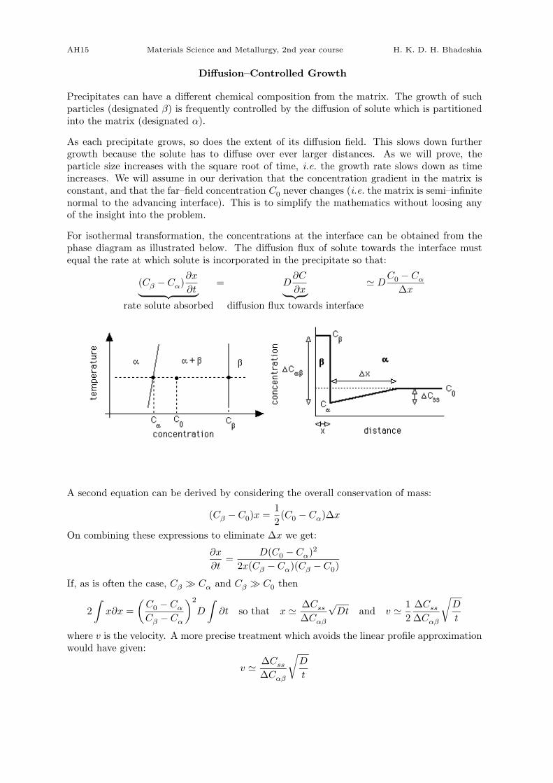
Diffusion–Controlled Growth

Precipitates can have a different chemical composition from the matrix. The growth of suchparticles (designated β) is frequently controlled by the diffusion of solute which is partitionedinto the matrix (designated α).

As each precipitate grows, so does the extent of its diffusion field. This slows down furthergrowth because the solute has to diffuse over ever larger distances. As we will prove, theparticle size increases with the square root of time, i.e. the growth rate slows down as timeincreases. We will assume in our derivation that the concentration gradient in the matrix isconstant, and that the far–field concentration C0 never changes (i.e. the matrix is semi–infinitenormal to the advancing interface). This is to simplify the mathematics without loosing anyof the insight into the problem.

For isothermal transformation, the concentrations at the interface can be obtained from thephase diagram as illustrated below. The diffusion flux of solute towards the interface mustequal the rate at which solute is incorporated in the precipitate so that:

(Cβ − Cα)∂x

∂t︸︷︷︸rate solute absorbed

= D∂C

∂x︸︷︷︸diffusion flux towards interface

' DC0 − Cα∆x

A second equation can be derived by considering the overall conservation of mass:

(Cβ − C0)x =1

2(C0 − Cα)∆x

On combining these expressions to eliminate ∆x we get:

∂x

∂t=

D(C0 − Cα)2

2x(Cβ − Cα)(Cβ − C0)

If, as is often the case, Cβ À Cα and Cβ À C0 then

2

∫x∂x =

(C0 − CαCβ − Cα

)2

D

∫∂t so that x ' ∆Css

∆Cαβ

√Dt and v ' 1

2

∆Css∆Cαβ

√D

t

where v is the velocity. A more precise treatment which avoids the linear profile approximationwould have given:

v ' ∆Css∆Cαβ

√D

t


Twinning in Cubic–Close–Packed Structure

Metals and Alloys - Phase Transformations and Complex ... · AH1 Materials Science and Metallurgy,...

Documents

Transcript of Metals and Alloys - Phase Transformations and Complex ... · AH1 Materials Science and Metallurgy,...