Mach Learn (2018) 107:285–311https://doi.org/10.1007/s10994-017-5685-x

Meta-QSAR: a large-scale application of meta-learningto drug design and discovery

Ivan Olier1,2 · Noureddin Sadawi3,4 · G. Richard Bickerton5,6 ·Joaquin Vanschoren7 · Crina Grosan4,8 · Larisa Soldatova4,9 · Ross D. King2

Received: 9 May 2016 / Accepted: 4 October 2017 / Published online: 22 December 2017© The Author(s) 2017. This article is an open access publication

Abstract We investigate the learning of quantitative structure activity relationships (QSARs)as a case-study of meta-learning. This application area is of the highest societal importance,as it is a key step in the development of newmedicines. The standard QSAR learning problem

Editors: Pavel Brazdil and Christophe Giraud-Carrier.

B Crina Grosancrina.grosan@brunel.ac.uk

Ivan Olieri.olier@mmu.ac.uk

Noureddin Sadawin.sadawi@imperial.ac.uk

G. Richard Bickertong.r.bickerton@dundee.ac.uk; rbickerton@exscientia.co.uk

Joaquin Vanschorenj.vanschoren@tue.nl

Larisa Soldatovalarisa.soldatova@brunel.ac.uk

Ross D. Kingr.king@manchester.ac.uk

1 Manchester Metropolitan University, Manchester, UK

2 University of Manchester, Manchester, UK

3 Imperial College London, London, UK

4 Brunel University London, London, UK

5 Dundee University, Dundee, UK

6 Exscientia Ltd, Dundee, UK

7 Eindhoven University of Technology, Eindhoven, The Netherlands

8 Babes-Bolyai University, Cluj-Napoca, Romania

9 Goldsmiths, University of London, London, UK

123

286 Mach Learn (2018) 107:285–311

is: given a target (usually a protein) and a set of chemical compounds (small molecules) withassociated bioactivities (e.g. inhibition of the target), learn a predictive mapping frommolec-ular representation to activity. Although almost every type of machine learning method hasbeen applied to QSAR learning there is no agreed single best way of learning QSARs, andtherefore the problem area is well-suited to meta-learning. We first carried out the most com-prehensive ever comparison of machine learning methods for QSAR learning: 18 regressionmethods, 3 molecular representations, applied to more than 2700 QSAR problems. (Theseresults have been made publicly available on OpenML and represent a valuable resource fortesting novel meta-learning methods.) We then investigated the utility of algorithm selec-tion for QSAR problems. We found that this meta-learning approach outperformed the bestindividual QSAR learning method (random forests using a molecular fingerprint representa-tion) by up to 13%, on average. We conclude that meta-learning outperforms base-learningmethods for QSAR learning, and as this investigation is one of the most extensive ever com-parisons of base and meta-learning methods ever made, it provides evidence for the generaleffectiveness of meta-learning over base-learning.

Keywords Meta-learning · Algorithm selection · Drug discovery · QSAR

1 Introduction

The standard approach to predicting how active a chemical compound will be against a giventarget (usually a protein that needs to be inhibited) in the development of new medicines is touse machine learning models. Currently, there is no agreed single best learning algorithm todo this. In this paper we investigate the utility of meta-learning to address this problem. Weaim to discover and exploit relationships between machine learning algorithms, measurableproperties of the input data, and the empirical performance of learning algorithms, to inferthe best models to predict the activity of chemical compounds on a given target.

1.1 Quantitative structure activity relationship (QSAR) learning

Drug development is one of themost important applications of science, as it is an essential stepin the treatment of almost all diseases. Developing a new drug is however slow and expensive.The average cost to bring a new drug to market is >2.5 billion US dollars (DiMasi et al.2015), which means that tropical diseases such as malaria, schistosomiasis, Chagas’ disease,etc., which kill millions of people and infect hundreds of millions of others are ‘neglected’(Ioset and Chang 2011; Leslie and Inouye 2011) and that ‘orphan’ diseases (i.e. those withfew sufferers) remain untreatable (Braun et al. 2010). More generally, the pharmaceuticalindustry is struggling to copewith spiralling drug discovery and development costs (Pammolliet al. 2011). Drug development is also slow, generally taking more than 10years. This meansthat there is strong pressure to speed up development, both to save lives and reduce costs. Asuccessful drug can earn billions of dollars a year, and as patent protection is time-limited,even one extra week of patent protection can be of great financial significance.

A key step in drug development is learning Quantitative Structure Activity Relationships(QSARs) (Martin 2010;Cherkasov et al. 2014;Cumming et al. 2013). These are functions thatpredict a compound’s bioactivity from its structure. The standard QSAR learning problemis: given a target (usually a protein) and a set of chemical compounds (small molecules) withassociated bioactivities (e.g. inhibiting the target), learn a predictive mapping frommolecularrepresentation to activity.

123

Mach Learn (2018) 107:285–311 287

Fig. 1 Rice’s framework foralgorithm selection. Adaptedfrom Rice (1976) andSmith-Miles (2008)

Although almost every form of statistical and machine learning method has been appliedto learning QSARs, there is no agreed single best way of learning QSARs. Therefore animportant motivation for this work is to better understand the performance characteristicsof the main (baseline) machine learning methods currently used in QSAR learning. Thisknowledge will feed into a better understanding of the performance characteristics of thesealgorithms, and will enable QSAR practitioners to improve there predictions.

The central motivation for this work is to better understand meta-learning through a case-study in the very important real-world application area of QSAR learning. This applicationarea is an excellent test-bed for the development of meta-learningmethodologies. The impor-tance of the subject area means that there are now thousands of publicly available QSARdatasets, all with the same basic structure. Few machine learning application areas haveso many datasets—enabling statistical confidence in meta-learning results. In investigatingmeta-learning we have focused on algorithm selection as this is the simplest form of meta-learning, and its use fits in with our desire to better understand the baseline-learningmethods.

A finalmotivation for thework is to improve the predictive performance ofQSAR learningthrough use of meta-learning. Our hope is that improved predictive performance will feedinto faster and cheaper drug development.

To enable others to build on our base-learning and meta-learning work we have placed allour results in OpenML.

1.2 Meta-learning: algorithm selection

Meta-learning has been used extensively to select themost appropriate learning algorithmon agiven dataset. In this section, we first sketch a general framework for algorithm selection, andthen provide an overview of prior approaches and the state-of-the-art in selecting algorithmsusing meta-learning.

1.2.1 Algorithm selection framework

The algorithm selection framework contains four main components: First, we construct theproblem space P , in our case the space of all QSAR datasets. Each dataset expresses theproperties and activity of a limited set of molecular compounds (drugs) on a specific targetprotein. In this paper, we consider 8292 QSAR datasets, described in more detail in Sect. 2.2.Second, we describe each QSAR dataset in P with a set of measurable characteristics (meta-features), yielding the feature space F . In this paper we include two types of meta-features:those that describe the QSAR data itself (e.g. the number of data points), and those thatdescribe properties of the target protein (e.g. hydrophobicity). We expect that these proper-ties will affect the interplay of different QSAR features, and hence the choice of learningalgorithm. The full set of meta-features used in this paper is described in Sect. 3.

123

288 Mach Learn (2018) 107:285–311

Third, the algorithm space A is created by the set of all candidate base-level learningalgorithms, in our case a set of 18 regression algorithms combined with several preprocessingsteps. These are described in Sect. 2.1.

Finally, the performance space Y represents the empirically measured performance, e.g.root mean squared error (RMSE) (Witten and Frank 2005) of each algorithm A on each ofthe QSAR datasets in P .

In the current state-of-the-art, there exists a wide variety of algorithm selection algorithms.If only a single algorithm should be run, we can train a classificationmodel that makes exactlythat prediction (Pfahringer et al. 2000; Guerri andMilano 2012).We can also use a regressionalgorithm to predict the performance of each algorithm (Xu et al. 2008), build a ranking ofpromising algorithms (Leite et al. 2012), or use cost-sensitive techniques which allow us tooptimize the loss we really care about in the end (Bischl et al. 2012; Xu et al. 2012).

Our task is: for any givenQSAR problem x ∈ P , select the best combination of QSAR andmolecular representation a ∈ A that maximizes a predefined performance measure y ∈ Y .In this paper, we investigate two meta-learning approaches: (1) classification problem: theaim is to learn a model that captures the relationship between the properties of the QSARdatasets, or meta-data, and the performance of the regression algorithms. This model canthen be used to predict the most suitable algorithm for a new dataset. (2) ranking problem:the aim is to fit a model that ranks the QSAR combinations by their predicted performances.

1.2.2 Previous work on algorithm selection using meta-learning

Meta-features In the meta-learning literature much effort has been devoted to the develop-ment of meta-features that effectively describe the characteristics of the data. These shouldhave discriminative power, meaning that they should be able to distinguish between base-learners in terms of their performance, and have a low computational complexity—preferablylower than O(n log n) (Pfahringer et al. 2000). Meta-features are typically categorised as oneof the following: simple (e.g. number of data points, number of features), statistical (e.g.meanstandard deviation of attributes, mean kurtosis of attributes, mean skewness of attributes), orinformation theoretic (e.g. mean entropy of the features, noise–signal ratio). See Bickel et al.(2008), Kalousis (2002) andVanschoren (2010) for an extensive description ofmeta-features.A subset of these may be used for regression, and some measures are specifically definedfor regression targets (Soares et al. 2004). Other meta-features can be trivially adapted to theregression data. First, landmarking (Pfahringer et al. 2000) works by training and evaluatingsets of simple, fast algorithms on the datasets (e.g. a decision stump instead of a full decisiontree), and using their performance (e.g. RMSE) as meta-features for the dataset. An analysisof landmarkers for regression problems can be found in Ler et al. (2005).

Another approach is to use model-based characteristics (Peng et al. 2002), obtained bybuilding fast, interpretable models, e.g. decision trees, and then extracting properties of thosemodels, such as the width, the depth and the number of leaves in the tree, and statisticalproperties (min, max, mean, stdev) of the distribution of nodes in each level of the tree,branch lengths, or occurrences of features in the splitting tests in the nodes. Recent researchon finding interestingways tomeasure data characteristics includes instance-level complexity(Smith et al. 2014a), measures for unsupervised learning (Lee and Giraud-Carrier 2011), anddiscretized meta-features (Lee and Giraud-Carrier 2008).

Meta-learning has also been successfully applied in stream mining (van Rijn et al. 2015b,2014) and time series analysis (Prudêncio and Ludermir 2004), each time requiring novelsets of meta-features.

123

Mach Learn (2018) 107:285–311 289

Selecting algorithms In meta-learning, algorithm selection is traditionally seen as a learningproblem: train a meta-learner that predicts the best algorithm(s) given a set of meta-featuresdescribing the data. In the setting of selecting a best single algorithm, experiments on artificialdatasets showed that there is no single best meta-learner, but that decision tree-like algorithms(e.g. C5.0boost) seem to have an edge, especiallywhen used in combinationwith landmarkers(Bensusan and Giraud-Carrier 2000; Pfahringer et al. 2000). Further experiments performedon real-world data corroborated these results, although they also show thatmostmeta-learnersare very sensitive to the exact combination of meta-features used (Köpf et al. 2000).

In the setting of recommending a subset of algorithms it was shown that, when using statis-tical and information-theoretical meta-features, boosted decision trees obtained best results(Kalousis 2002; Kalousis and Hilario 2001). Relational case-based reasoning has also beensuccessfully applied (Lindner and Studer 1999; Hilario and Kalousis 2001), which allowsto include algorithm properties independent of the dataset and histogram representations ofdataset attribute properties.

Most relevant for this paper is the work by Amasyali and Ersoy (2009), which usesaround 200 meta-features to select the best regression algorithm for a range of artificial,benchmarking, and drug discovery datasets. The reported correlations betweenmeta-featuresand algorithmperformanceswere typically above 0.9 on artificial and benchmarking datasets,but much worse (below 0.8) on the drug discovery datasets. Feature selection was found tobe important to improve meta-learning performance.

Ranking algorithms Another approach is to build a ranking of algorithms, listing whichalgorithms to try first. Several techniques use k-nearest neighbors (Brazdil et al. 2003; dosSantos et al. 2004), and compute the average rank (or success rate ratio’s or significant wins)over all similar prior datasets (Soares and Brazdil 2000; Brazdil and Soares 2000). Otherapproaches directly estimate the performances of all algorithms (Bensusan and Kalousis2001), or use predictive clustering trees (Todorovski et al. 2002).

Better results were obtained by subsampling landmarkers, i.e. running all candidate algo-rithms on several small samples of the new data (Fürnkranz and Petrak 2001). Meta-learningon data samples (MDS) (Leite andBrazdil 2005, 2007) builds on this idea by first determiningthe complete learning curves of a number of learning algorithms on several different datasets.Then, for a new dataset, progressive subsampling is done up to a certain point, creating apartial learning curve, which is then matched to the nearest complete learning curve for eachalgorithm in order to predict their final performances on the entire new dataset.

Another approach is to sequentially evaluate a few algorithms on the (complete) newdataset and learn from these results.Active testing (Leite et al. 2012) proceeds in a tournament-style fashion: in each round it selects and tests the algorithm that is most likely to outperformthe current best algorithm, based on a history of prior duels between both algorithms onsimilar datasets. Each new test will contribute information to a better estimate of datasetsimilarity, and thus help to better predict which algorithms are most promising on the newdataset. Large-scale experiments show that active testing outperforms previous approaches,and yields an algorithm whose performance is very close to the optimum, after relatively fewtests. More recent work aims to speed up active testing by combining it with learning curves(vanRijn et al. 2015a), so that candidate algorithmsonly need to be trainedon a smaller sampleof the data. It also uses a multi-objective criterion called AR3 (Abdulrahman and Brazdil2014) that trades off runtime and accuracy so that fast but reasonably accurate candidatesare evaluated first. Experimental results show that this method converges extremely fast toan acceptable solution.

123

290 Mach Learn (2018) 107:285–311

Finally, algorithms can also be ranked using collaborative filtering (Bardenet et al. 2013;Misir and Sebag 2013; Smith et al. 2014b). In this approach, previous algorithm evaluationsare used as ‘ratings’ for a given dataset. For a new dataset, algorithms which would likelyperform well (give a high rating) are selected based on collaborative filtering models (e.g.using matrix decompositions).

Model-based optimization Model-based optimization (Hutter et al. 2011) aims to select thebest algorithm and/or best hyperparameter settings for a given dataset by sequentially evalu-ating them on the full dataset. It learns from prior experiments by building a surrogate modelthat predicts which algorithms and parameters are likely to perform well. An approach thathas proven to work well in practice is Bayesian Optimization (Brochu et al. 2010), whichbuilds a surrogate model (e.g. using Gaussian Processes or Random Forests) to predict theexpected performance of all candidate configurations, as well as the uncertainty of that pre-diction. In order to select the next candidate to evaluate, an acquisition function is usedthat trades off exploitation (choosing candidates in regions known to perform well) versusexploration (trying candidates in relatively unexplored regions). Bayesian Optimization isused in Auto-WEKA (Thornton et al. 2013) and Auto-sklearn (Feurer et al. 2015), whichsearch for the optimal algorithms and hyperparameters across the WEKA (Hall et al. 2009)and scikit-learn (Pedregosa et al. 2011) environments, respectively. Given that this techniqueis computationally very expensive, recent research has tried to include meta-learning to finda good solution faster. One approach is to find a good set of initial candidate configurationsby using meta-learning (Feurer et al. 2015): based on meta-features, one can find the mostsimilar datasets and use the optimal algorithms and parameter settings for these datasets asthe initial candidates to evaluate. In effect, this provides a ‘warm start’ which yields betterresults faster.

1.3 Meta-QSAR learning

Almost every form of statistical and machine learning method has been applied to learn-ing QSARs: linear regression, decision trees, neural networks, nearest-neighbour methods,support vector machines, Bayesian networks, relational learning, etc. These methods dif-fer mainly in the a a priori assumptions they make about the learning task. We focus onregression algorithms as this is how QSAR problems are normally cast.

For Meta-QSAR learning the input data are datasets of compound activity (one for eachtarget protein), different representations of the structures of the compounds, and we aimto learn to predict how well different learning algorithms perform, and to exploit thesepredictions to improve QSAR predictions. We expect meta-learning to be successful forQSAR because although all the datasets have the same overall structure, they differ in thenumbers of data points (tested chemical compounds), in the range and occurrence of features(compound descriptors), and in the type of chemical/biochemical mechanism that causes thebioactivity. These differences indicate that different machine learning methods are to be usedfor different kinds of QSAR data.

We first applied meta-learning to predict the machine learning algorithm that is expectedto perform best on a given QSAR dataset. This is known as the algorithm selection problem,and can be expressed formally using Rice’s framework for algorithm selection (Rice 1976) asillustrated in Fig. 1.We then appliedmulti-task learning to first test whether it can improve onstandard QSAR learning through the exploitation of evolutionary related targets, and whethermulti-task learning can further be improved by incorporating the evolutionary distance oftargets.

123

Mach Learn (2018) 107:285–311 291

1.4 Paper outline

The remainder of this paper is organized as follows. In Sect. 2, we report our baselineexperiments investigating the effectiveness of a large number of regression algorithms onthousands of QSAR datasets, using different data representations. In Sect. 3 we describe anovel set ofQSAR-specificmeta-features to inform ourmeta-learning approach. In Sect. 4weinvestigate the utility of meta-learning for selecting the best algorithm for learning QSARs.Finally, Sect. 5 presents a discussion of our results and future work.

2 Baseline QSAR learning

Wefirst performed experimentswith a set of baseline regression algorithms to investigate theireffectiveness on QSAR problems. Learning a QSAR model consists of fitting a regressionmodel to a dataset which has as instances the chemical compounds, as input variables thechemical compound descriptors, and as numeric response variable (output) the associatedbioactivities.

2.1 Baseline QSAR learning algorithms

For our baseline QSAR methods we selected 18 regression algorithms, including linearregression, support vector machines, artificial neural networks, regression trees, and randomforests. Table 1 lists all the algorithms used and their respective parameter settings. Withinthe scope of this study, we do not optimize the parameter settings on every dataset, but insteadchose values that are likely to perform well on most QSAR datasets. This list includes themost commonly used QSAR methods in the literature.

With the exception of one of the neural networks implementations, for which we usedthe H2O R package,1 all of the algorithms were implemented using the MLR R package formachine learning.2

2.2 Baseline QSAR datasets

For many years, QSAR research was held back by a lack of openly available datasets. Thissituation has been transformed by a number of developments. The most important of these isthe open availability of the ChEMBL database,3 a medicinal chemistry database managed bythe European Bioinformatics Institute (EBI). It is abstracted and curated from the scientificliterature, and covers a significant fraction of themedicinal chemistry corpus. The data consistof information on the drug targets (mainly proteins from a broad set of target families, e.g.kinases), the structures of the tested compounds (from which different chemoinformaticrepresentations may be calculated), and the bioactivities of the compounds on their targets,such as binding constants, pharmacology, and toxicity. The key advantages of usingChEMBLfor Meta-QSAR are: (a) it covers a very large number of targets, (b) the diversity of thechemical space investigated, and (c) the high quality of the interaction data. Itsmainweaknessis that for any single target, interaction data on only a relatively small number of compoundsare given.

1 https://cran.r-project.org/web/packages/h2o/index.html.2 https://cran.r-project.org/web/packages/mlr/index.html.3 https://www.ebi.ac.uk/chembl/.

123

292 Mach Learn (2018) 107:285–311

Table1

Listo

fbaselin

eQSA

Ralgorithms

Shortn

ame

Nam

eParameter

settings

ctree

Con

ditio

naltrees

min_split

=20,

min_bucket=

7

rtree

Regressiontrees

min_split

=20,

min_bucket=

7

cforest

Random

forest(w

ithconditionaltrees)

n_trees=

500,min_split

=20,

min_bucket=

7

rforest

Rando

mforest

n_trees=

500,min_split

=20,

min_bucket=

7

gbm

Generalized

boostedregression

n_trees=

100,depth=1

,CV

=no,min_o

bs_n

ode=1

0

fnn

k-Nearestneighb

ork=1

earth

Adaptiveregression

splin

es(earth)

(Asdefault)

glmnet

Regularized

GLM

(Asdefault)

ridge

Penalized

ridgeregression

(Asdefault)

lmMultip

lelin

earregression

(Asdefault)

pcr

Principalcom

ponent

regression

(Asdefault)

plsr

Partialleastsquares

(Asdefault)

rsm

Responsesurfaceregression

(Asdefault)

rvm

Relevance

vector

machine

Kernel=

RBF,nu

=0.2,epsilo

n=0

.1

ksvm

Supp

ortv

ectormachines

Kernel=

RBF,nu

=0.2,epsilo

n=0

.1

ksvm

fpSu

pportv

ectormachineswith

Tanimotokernel

Kernel=

Tanimoto

nnet

Neuraln

etworks

size

=3nn

eth2

oNeuraln

etworks

usingH2O

library

layers

=2,sizelayer1=0

.333

*n_

inpu

ts,layer

2=0

.667

*n_inp

uts

n_treesnu

mberof

trees;min_splitminim

umnode

size

allowed

forsplittin

g;min_bucketminim

umsize

ofthebucket.k

numberof

neighb

ours;depthsearch

depth;

CVcross-

valid

ation;

min_o

bs_n

odeminim

umnu

mberof

observations

perno

de;R

BFradialbasisfunctio

nwith

nu(spread)

andepsilon(scale)parameters;size

numberof

neuron

sin

the

hidd

enlayer;n_

inpu

tsleng

thof

theinpu

tvector

123

Mach Learn (2018) 107:285–311 293

Table 2 Names of the generated dataset representations

Basic set of descriptors (43) All descriptors (1447) FCFP4 fingerprint (1024)

Original dataset basicmolprop (not used) allmolprop (not used) fpFCFP4

Missing value imputation basicmolprop.miss allmolprop.miss (No missing values)

We extracted 2764 targets from ChEMBLwith a diverse number of chemical compounds,ranging from 10 to about 6000, each target resulting in a dataset with as many examples ascompounds. The target (output) variable contains the associated bioactivities. Bioactivity datawere selected on the basis that the target type is a protein, thereby excluding other potentialtargets such as cell-based and in vivo assays, and the activity type is from a defined list ofpotency/affinity endpoints (IC50, EC50,Ki, Kd and their equivalents). In the small proportionof cases where multiple activities have been reported for a particular compound-target pair,a consensus value was selected as the median of those activities falling in the modal log unit.The simplified molecular-input line-entry system (SMILES) representation of the moleculeswas used to calculate molecular properties such as molecular weight (MW), logarithm ofthe partition coefficient (LogP), topological polar surface area (TPSA), etc. For this we usedDragon version 6 (Mauri et al. 2006), which is a commercially available software library thatcan potentially calculate up to 4885 molecular descriptors, depending on the availability of3D structural information of the molecules. A full list is available on Dragon’s website.4

As ChEMBL records 2D molecular structures only, we were restricted to estimating amaximum of 1447 molecular descriptors. We decided to generate datasets using all per-mitted molecular descriptors as features, and then to extract a subset of 43, which Dragonidentifies as basic or constitutional descriptors. We call these representations ‘allmolprop’and ‘basicmolprop’, respectively. For some of the molecules, Dragon failed to compute someof the descriptors, possibly because of bad or malformed structures, and these were treatedas missing values. To avoid favouring QSAR algorithms able to deal with missing values, wedecided to impute them, as a preprocessing step, using the median value of the correspondingfeature.

In addition, we calculated the FCFP4 fingerprint representation using the Pipeline Pilotsoftware from BIOVIA (Rogers and Hahn 2010). The fingerprint representation is the mostcommonly used inQSAR learning, whereby the presence or absence of a particularmolecularsubstructure in amolecule (e.g.methyl group, benzine ring) is indicated by aBooleanvariable.The FCFP4 fingerprint implementation generates 1024 such Boolean variables. We call thisdataset representation ‘fpFCFP4’. All of the fpFCFP4 datasets were complete, so a missingvalue imputation step is not necessary.

In summary, we use 3 types of feature representations and 1 level of preprocessing, thusgenerating 3 different dataset representations for each of the QSAR problems (targets), seeTable 2. This produced in total 8292 datasets from the 2764 targets.

2.3 Baseline QSAR experiments

The predictive performance of all the QSAR learning methods on the datasets (base QSARexperiments) was assessed by taking the average root mean squared error (RMSE) withtenfold cross-validation.

4 http://www.talete.mi.it.

123

294 Mach Learn (2018) 107:285–311

Fig. 2 Graphical representation of the number of times (target counts) a particular QSAR learning methodobtains the best performance (minimum RMSE)

Fig. 3 Graphical representationof the number of times (targetcounts) a dataset representationwas fitted with the best performerQSAR method (minimumRMSE)

We used the parameter settings mentioned in Table 1 for all experiments. Figure 2 summa-rizes the overall relative performance (in frequencies) of the QSAR methods for all datasetrepresentations previously mentioned in Table 2. Results showed that random forest (‘rfor-est’) was the best performer in 1162 targets out of 2764, followed by SVM (‘ksvm’), 298targets, and GLM-NET (‘glmnet’), 258 targets. In these results, the best performer is thealgorithm with the lowest RMSE, even if it wins by a small margin. In terms of datasetrepresentation, it turned out that datasets formed using FCFP4 fingerprints yielded consis-tently better models than the rest of the datasets (in 1535 out of 2764 situations). Results aredisplayed in Fig. 3.

Figure 4 summarizes the results obtained using various strategies (combinations of QSARalgorithm and dataset representation). As the figure shows, the bar plot is highly skewedtowards the top ranked QSAR strategies with a long tail representing QSAR problems inwhich other algorithms perform better.

Applying random forest to datasets formed using either FCFP4 fingerprints or all molec-ular properties were the most successful QSAR strategies (in the figure, rforest.fpFCFP4for 675 and rforest.allmolprop.miss for 396 out of 2764 targets, respectively). Other strate-gies, such as regression with ridge penalisation (ridge.fpFCFP4), SVMwith Tanimoto kernel(ksvmfp.fpFCFP4), and SVM with RBF kernel (ksvm.fpFCFP4) were particularly success-ful when using the FCFP4 fingerprint dataset representation (for 154, 141, and 126 targets,

123

Mach Learn (2018) 107:285–311 295

Fig. 4 Graphical representation of the number of times (target counts) a combination of dataset representationand QSAR method obtained the best performance (minimum RMSE)

respectively). The full list of strategies ranked by frequency of success is shown in the figure.Combinations that never produced best performances are not shown.

Combinations of QSARs and representations were also ranked by their average perfor-mances. For this, we estimated an averageRMSE ratio score (aRMSEr)which is adapted fromBrazdil et al. (2003), originally introduced for classification tasks. Our score was formulatedas follows:

aRMSErp =∑

qn√∏

i RMSErip,q

m

where RMSErip,q = RMSEiq/RMSEi

p is the (inverse) RMSE ratio between algorithmsp and q for the dataset i . In the same equation, m represents the number of algorithms,whilst n, the number of targets. Notice that, an RMSErip,q > 1 indicates that algorithm poutperformed algorithm q . Ranking results using aRMSEr are presented in Fig. 5.

We ran a Friedman test with a corresponding pairwise post-hoc test (Demsar 2006), whichis a non-parametric equivalent of ANOVA in order to verify whether the performances of

123

296 Mach Learn (2018) 107:285–311

Fig. 5 Average ranking of dataset representation and QSAR combination as estimated using the RMSE ratio

baseline QSAR strategies were statistically different. The Friedman test ranks the strategiesused per dataset according to their performance and tests them against the null hypothesisthat they are equivalent. A post-hoc test was carried out if the null hypothesis is rejected.For this we used the Nemenyi test, also suggested by Demsar (2006). The resulting P value(10E−06) from the test indicates the null hypothesis was invalid (P value << 0.05), whichsuggests that algorithm selection should significantly impact the overall performance.

We ran the aforementioned post-hoc test for the top 6 QSAR strategies5 presented inFig. 5. Results are shown in Fig. 6. It shows that performance differences between the QSARstrategies were statistically significant with the exception of rforest.allmolprop.miss versusksvmfp.fpFCFP4.

5 Testing all possible pairwise combinations of QSAR strategies was not possible as the post-hoc test wasrunning extremely slowly and we considered it would not add to the analyses of the results.

123

Mach Learn (2018) 107:285–311 297

Fig. 6 Box plot displays the post-hoc test results over the top 6 ranked best performer QSAR strategies: 1—rforest.fpFCFP4, 2—ksvm.fpFCFP4, 3—ksvmfp.fpFCFP4, 4—rforest.allmolprop.miss, 5—glmnet.fpFCFP4,and 6—rforest.basicmolprop.miss.fs. Statistically significant comparisons (P value < 0.05) represented withgreen boxes (Color figure online)

3 Meta-features for meta-QSAR learning

3.1 Meta-QSAR ontology

Meta-learning analysis requires a set of meta-features. In our meta-QSAR study we usedas meta-features, characteristics of the datasets considered in the base study and drug targetproperties. We utilised a similar approach employed by BODO (the Blue Obelisk DescriptorOntology) (Floris et al. 2011) and the Chemical Information Ontology (Hastings et al. 2011)for the formal definitions of molecular descriptors used in QSAR studies, and developed ameta-QSAR ontology.6

The meta-QSAR ontology provides formal definitions for the meta-features used in thereportedmeta-QSAR study (see Fig. 7). Themeta-features are defined at the conceptual level,meaning that the ontology does not contain instance-level values of meta-features for eachof 8292 considered dataset. For example, the meta-feature ’multiple information’ is definedas the meta-feature of a dataset (multiple information (also called total correlation) amongthe random variables in the dataset), but the meta-QSAR ontology does not contain valuesof this meta-feature for each dataset. Instead, it contains links to the code to calculate valuesof the relevant features. For example, we used the R Package Peptides7 to calculate valuesof the meta-feature ‘hydrophobicity’. Figure 8 shows how this information is captured in themeta-QSAR ontology. The description of the selected meta-features and instructions on thecalculation of their values are available online.8

3.2 Dataset meta-features

The considered8292datasets have a rangeof different properties, e.g. ’number of compounds’(instances) in the dataset, ’entropy’ and ’skewness’ of the features and ’target meta-feature’,’mutual information’ and ’total correlation’ between the input and output features (see Table 3

6 The ontology is available at https://github.com/larisa-soldatova/meta-qsar.7 http://cran.r-project.org/web/packages/Peptides/.8 https://github.com/meta-QSAR/drug-target-descriptors.

123

298 Mach Learn (2018) 107:285–311

Fig. 7 The key branches of the meta-QSAR ontology (a fragment)

Fig. 8 The representation of the meta-features and their values

for more detail). The dataset properties have a significant effect on the performance of theexplored algorithms and were used for the meta-QSAR learning. Figure 11 shows the levelof influence of different categories of meta-features. For example information-theoreticalmeta-features make a considerable contribution to meta-learning.

Some descriptors of the dataset properties, e.g. ’number of instances’, have been importedfrom the Data Mining Optimization (DMOP) Ontology9 (Keeta et al. 2015). We also addedQSAR-specific dataset descriptors ’aggregated fingerprint’. These were calculated by sum-ming1s (set bits) in each of the 1024 columns andnormalised by the number of the compoundsin each dataset.

9 www.dmo-foundry.org/DMOP.

123

Mach Learn (2018) 107:285–311 299

Table 3 Dataset meta-features (examples)

Feature Description

multiinfo Multiple information (also called total correlation)among the random variables in the dataset

mutualinfo Mutual information between nominal attributes X andY. Describes the reduction in uncertainty of Y due tothe knowledge of X, and leans on the conditionalentropy H(Y |X)

nentropyfeat Normalised entropy of the features which is the classentropy divided by log(n) where n is the number of thefeatures

mmeanfeat Average mean of the features

msdfeat Average standard deviation of the features

kurtresp Kurtosis of the response variable

meanresp Mean of the response variable

skewresp Skewness of the response variable

nentropyresp Normalised entropy of the response variable

sdresp Standard deviation of the response

aggFCFP4fp (1024 features) Aggregated fingerprints and normalized over thenumber of instances in the dataset

3.3 Drug target meta-features

3.3.1 Drug target properties

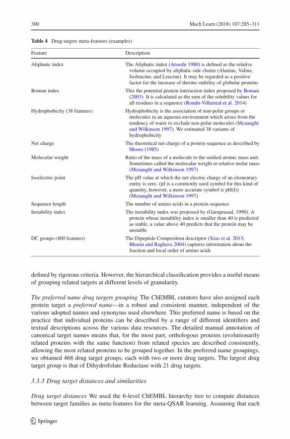
TheQSAR datasets are additionally characterized bymeasurable properties of the drug target(a protein) they represent, such as ’aliphatic index’, ’sequence length’, ’isoelectric point’ (seeTable 4 for more details). These differ from the molecular properties we used to describe thechemical compounds in the QSAR dataset instances, e.g. ’molecular weight’ (MW), ’LogP’.

3.3.2 Drug target groupings

Wealso used drug target groupings (Imming et al. 2006), such as ’drug target classes’, and ’thepreferred name groupings’, as meta-features. These enable meta-learning to exploit knownbiological/chemical relationships between the targets (proteins). Indeed, if the target proteinsare similar, this may make the resulting datasets more similar too.

Drug target classes The ChEMBL database curators have classified the protein targets in amanually curated family hierarchy. The version of the hierarchy that we have used (takenfrom ChEMBL20) comprises 6 levels, with Level 1 (L1) being the broadest class, and Level6 (L6) the most specific. For example, the protein target ‘Tyrosine-protein kinase Srms’ isclassified as follows:Enzyme (L1),Kinase (L2), ProteinKinase (L3), TKprotein kinase group(L4), Tyrosine protein kinase Src family (L5), Tyrosine protein kinase Srm (L6). Differentclasses in Level 1 are not evolutionarily related to one another, whereas members of classesin L3 and below generally share common evolutionary origins. The picture is mixed for L2.The hierarchy is not fully populated, with the greatest emphasis being placed on the targetfamilies of highest pharmaceutical interest, and the different levels of the hierarchy are not

123

300 Mach Learn (2018) 107:285–311

Table 4 Drug targets meta-features (examples)

Feature Description

Aliphatic index The Aliphatic index (Atsushi 1980) is defined as the relativevolume occupied by aliphatic side chains (Alanine, Valine,Isoleucine, and Leucine). It may be regarded as a positivefactor for the increase of thermo stability of globular proteins

Boman index This the potential protein interaction index proposed by Boman(2003). It is calculated as the sum of the solubility values forall residues in a sequence (Rondn-Villarreal et al. 2014)

Hydrophobicity (38 features) Hydrophobicity is the association of non-polar groups ormolecules in an aqueous environment which arises from thetendency of water to exclude non-polar molecules (Mcnaughtand Wilkinson 1997). We estimated 38 variants ofhydrophobicity

Net charge The theoretical net charge of a protein sequence as described byMoore (1985)

Molecular weight Ratio of the mass of a molecule to the unified atomic mass unit.Sometimes called the molecular weight or relative molar mass(Mcnaught and Wilkinson 1997)

Isoelectric point The pH value at which the net electric charge of an elementaryentity is zero. (pI is a commonly used symbol for this kind ofquantity, however, a more accurate symbol is pH(I))(Mcnaught and Wilkinson 1997)

Sequence length The number of amino acids in a protein sequence

Instability index The instability index was proposed by (Guruprasad, 1990). Aprotein whose instability index is smaller than 40 is predictedas stable, a value above 40 predicts that the protein may beunstable

DC groups (400 features) The Dipeptide Composition descriptor (Xiao et al. 2015;Bhasin and Raghava 2004) captures information about thefraction and local order of amino acids

defined by rigorous criteria. However, the hierarchical classification provides a useful meansof grouping related targets at different levels of granularity.

The preferred name drug targets grouping The ChEMBL curators have also assigned eachprotein target a preferred name—in a robust and consistent manner, independent of thevarious adopted names and synonyms used elsewhere. This preferred name is based on thepractice that individual proteins can be described by a range of different identifiers andtextual descriptions across the various data resources. The detailed manual annotation ofcanonical target names means that, for the most part, orthologous proteins (evolutionarilyrelated proteins with the same function) from related species are described consistently,allowing the most related proteins to be grouped together. In the preferred name groupings,we obtained 468 drug target groups, each with two or more drug targets. The largest drugtarget group is that of Dihydrofolate Reductase with 21 drug targets.

3.3.3 Drug target distances and similarities

Drug target distances We used the 6-level ChEMBL hierarchy tree to compute distancesbetween target families as meta-features for the meta-QSAR learning. Assuming that each

123

Mach Learn (2018) 107:285–311 301

(1024 features)

Problem space P

21 QSAR dataset properties

Meta-feature extraction

Meta-feature space F

452 target (protein) properties

52 QSAR combinations

(feature gen + preproc + learner)

Performance space Y

(random forest)

Evaluate

2764 QSAR datasets / targets

Feature generation

molecular prop. (1447 features)

MVI = Missing value imputation

8292 (3*2764) QSAR datasets

train

predict

18 regression algorithms

Algorithm space A

basic prop. (43 features)

Feature generation

Preprocessing: MVI, none

Preprocessing: MVI, none906 target family distances

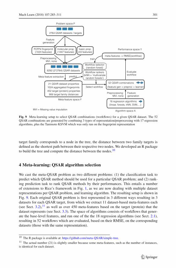
Fig. 9 Meta-learning setup to select QSAR combinations (workflows) for a given QSAR dataset. The 52QSAR combinations are generated by combining 3 types of representation/preprocessing with 17 regressionalgorithms, plus the Tanimoto KSVM which was only run on the fingerprint representation

target family corresponds to a node in the tree, the distance between two family targets isdefined as the shortest path between their respective two nodes. We developed an R packageto build the tree and compute the distance between the nodes.10

4 Meta-learning: QSAR algorithm selection

We cast the meta-QSAR problem as two different problems: (1) the classification task topredict which QSAR method should be used for a particular QSAR problem; and (2) rank-ing prediction task to rank QSAR methods by their performances. This entails a numberof extensions to Rice’s framework in Fig. 1, as we are now dealing with multiple datasetrepresentations per QSAR problem, and learning algorithm. The resulting setup is shown inFig. 9. Each original QSAR problem is first represented in 3 different ways resulting in 3datasets for each QSAR target, from which we extract 11 dataset-based meta-features each(see Sect. 3.2),11 as well as over 450 meta-features based on the target (protein) that thedataset represents (see Sect. 3.3). The space of algorithms consists of workflows that gener-ate the base-level features, and run one of the the 18 regression algorithms (see Sect. 2.1),resulting in 52 workflows which are evaluated, based on their RMSE, on the correspondingdatasets (those with the same representation).

10 The R package is available at: https://github.com/meta-QSAR/simple-tree.11 The actual number (21) is slightly smaller because some meta-features, such as the number of instances,is identical for each dataset.

123

302 Mach Learn (2018) 107:285–311

Fig. 10 Schematic representation of the meta-dataset used for meta-QSAR

4.1 Meta-QSAR dataset

A training meta-dataset was formed using the meta-features extracted from the baselineQSAR datasets as the inputs. For the classification tasks we used the best QSAR strategy(combination of QSAR method and dataset representation) per target as the output labels,whilst for the ranking tasks, the QSAR performances (RMSEs) were used. Figure 10 showsa schematic representation of the meta-dataset used in the meta-learning experiments. Asthis figure shows, we used meta-features derived from dataset and drug target properties. Thesize of the final meta-dataset was 2394 meta-features by 2764 targets.

4.2 Meta-QSAR learning algorithms

A meta-learning classification problem using all possible combinations of QSAR methodsand dataset representions was implemented using a random forest with 500 trees. Given thelarge number of classes (52 combinations) and the highly imbalanced classification problem(as shown in Fig. 4, additional random forest implementations using the top 2, 3, 6, 11and 16 combinations (Fig. 5) were also investigated. For the ranking problem, we used twoapproaches: K-nearest neighbour approach (k-NN), as suggested in Brazdil et al. (2003),and a multi-target regression approach. Experiments with k-NN were carried out using 1,5, 10, 50, 100, 500, and all neighbours. The multi-target regression was implemented usinga multivariate random forest regression (Segal and Xiao 2001) with 500 trees to predictQSAR performances and with them, to rank QSAR combinations. All implementations wereassessed using tenfold cross-validation.

4.3 Results

We used the all-classes random forest implementation to estimate the importance of eachmeta-feature in the classification task, as estimated using the mean decrease accuracy. Sum-mary results considered by meta-feature groups are presented in Fig. 11. It is seen thatthe meta-features belonging to the information theory group (all dataset meta-features butthe aggregated fingerprints, Table 3) were the most relevant, although we found all groupscontributed to the task.

As mentioned before, k-NN and multivariate random forest were used to implement rank-ing models. We used the Spearman’s rank correlation coefficient to compare the predictedwith the actual rankings (average of the actual rankingswere shown in Fig. 5). Results of thesecomparisons are shown in Fig. 12. It is observed from the figure that the multivariate randomforest and 50-nearest neighbours implementations (mRF and 50-NN in the figure) predicted

123

Mach Learn (2018) 107:285–311 303

Fig. 11 Violin plots with added box plots representing the mean decrease accuracy of the meta-featuresgrouped by meta-feature groups. Notice that for visualization purposes, we are showing the group datasetmeta-features (as defined in Sect. 3) in two separated groups: “Aggregated Fingerprints” and “InformationTheory”

Fig. 12 Box plots representing the computed Spearman’s rank correlation coefficient (rs) between the pre-dicted and actual rankings. Labels in the horizontal axis indicates: mRF—multivariate random forest, 1-NN,5-NN, 10-NN, 50-NN, 100-NN, 500-NN, and All—1, 5, 10, 50, 100, 500, and all nearest neighbours, respec-tively

better rankings, overall. For illustrative purpose, the average of the predicted rankings bymultivariate random forest is displayed in Fig. 13.

Performances of the best suggested QSAR combination by all Meta-QSAR implementa-tions were compared with an assumed default. In the case of the ranking models, the bestsuggested QSAR combination is the one ranked the highest in each QSAR problem. For

123

304 Mach Learn (2018) 107:285–311

Fig. 13 Average of predicted ranking of QSAR combinations using the multivariate random forest algorithmaccording to the RMSE ratio

the default (baseline) we used random forest with the fingerprint molecular representation(rforest.fpFCFP4 ), as this is well-known for its robust and reliable performance (Fig. 4), andhence represents a strong baseline. Results are shown in Fig. 14. As can be observed in thisfigure, most of the Meta-QSAR implementations improved overall performance in compar-ison with the default QSAR combination with the exception of the 1-nearest neighbour. Thesame results are summarized in Table 5. We ran a Wilcoxon Rank Sum tests on the RMSEdifferences between the Meta-QSAR implementations and the assumed default. Results, inthe form of P values, are also shown in the same table. According to these tests, performanceimprovements by Meta-QSAR implementations cl.Top11, cl.Top16, and cl.All were not sta-tistically significant (P value > 0.05). Overall, the results suggest that meta-learning can besuccessfully used to select QSAR algorithm/representation pairs that perform better than thebest algorithm/representation pair (default strategy).

123

Mach Learn (2018) 107:285–311 305

Fig. 14 Visual comparison ofperformance distributionsbetween the default strategy (inblack) and all meta-learners (ingrey) using asymmetric beanplots. Average RMSE for eachimplementation is represented byvertical black lines on the“beans” (performancedistribution curves)

Table 5 Comparison of performance between the default strategy and all Meta-QSAR implementations

Implementation Mean RMSE Relative RMSE reduction (%) P value

Default 0.1964

mRF 0.1709 13.0 < 0.001

All-NN 0.1737 11.6 < 0.001

500-NN 0.1738 11.5 < 0.001

100-NN 0.1738 11.5 0.009

50-NN 0.1751 10.9 0.003

10-NN 0.1815 7.6 0.011

5-NN 0.1881 4.3 < 0.001

1-NN 0.2098 − 6.8 < 0.001

cl.Top2 0.1711 12.9 0.007

cl.Top3 0.1709 13.0 < 0.001

cl.Top6 0.1779 9.5 0.022

cl.Top11 0.1771 9.9 0.086

cl.Top16 0.1788 9.0 0.072

cl.All 0.1823 7.2 0.189

Relative RMSE reduction (in%) is estimated as (mRMSEDef −mRMSEMQSAR)/mRMSEDef × 100%,where mRMSEDef and mRMSEMQSAR correspond to the mean RMSE of the default and Meta-QSARstrategies, respectively. P values were estimated using Wilcoxon Rank Sum test

5 Discussion

QSARmodels are regressionmodels, empirical functions that relate a quantitative descriptionof a chemical structure (a drug) to some form of biological activity (e.g. inhibiting proteins)for the purposes of informing drug design decision-making. Many consider the seminalpapers of Hansch and Fujita (1964) to be the origin of the QSAR field. Since then, such

123

306 Mach Learn (2018) 107:285–311

predictive modelling approaches have grown to become a core part of the drug discoveryprocess (Cumming et al. 2013; Cherkasov et al. 2014). The subject is still increasing inimportance (Cramer 2012). This may be attributed to the alignment of a number of factors,including increased availability of data, advances in data-mining methodologies as well as amore widespread appreciation of how to avoid many of the numerous pitfalls in building andapplying QSAR models (Cherkasov et al. 2014). Current trends in the field include effortsin chemical data curation (Williams et al. 2012), automation of QSAR model building (Coxet al. 2013), exploration of alternative descriptors (Cherkasov et al. 2014), and efforts to helpdefine the Applicability Domain (AD) of a given QSAR model (Sahigara et al. 2012).

To facilitate application of QSARmodels in the drug regulatory process, the Organizationfor Economic Co-operation and Development (OECD) has provided guidance to encouragegood practice inQSARmodelling. TheOECDguidelines recommend that aQSARmodel has(i) a defined end point; (ii) an unambiguous algorithm; (iii) a defined domain of applicability;(iv) appropriatemeasures of goodness of fit, robustness and predictivity; and (v) amechanisticinterpretation, if possible. However, the application of QSAR models in drug discovery isstill fraught with difficulties, not least because the model builder is faced with myriad optionswith respect to choice of descriptors and machine learning methods.

The application of meta-learning in this study helps ameliorate this issue by providingsome guidance as to which individual method performs the best overall as well as whichmethod may be the most appropriate given the particular circumstances.

Our comparison of QSAR learning methods involves 18 regression methods and 3 molec-ular representations applied to more than 2700 QSAR problems, making it one of the mostextensive ever comparisons of base learningmethods reported.Moreover, theQSARdatasets,source code, and all our experiments are available on OpenML (Vanschoren et al. 2013),12 sothat our results can be easily reproduced. This is not only a valuable resource for further workin drug discovery, it will foster the development of meta-learning methods as well. Indeed,as all the experimental details are fully available, there is no need to run the baseline-learnersagain, so research effort can be focused on developing novel meta-learning methods.

In this paper we have investigated algorithm selection for QSAR learning. Note how-ever, that many more meta-learning approaches could be applied: it would be interestingto investigate other algorithm selection methods (see Sect. 1.2.2), such as other algorithmranking approaches (e.g. active testing or collaborative filtering), and model-based optimiza-tion. Another alternative framing of the meta-learning problem would be to use a regressionalgorithm at the meta-level and predict the performance of various regression algorithms.We will explore this in future work. Finally, we would also like to explore other algorithmselection techniques beyond Random Forests. To this end, we plan to export our experimentsfrom OpenML to an ASlib scenario (Bischl et al. 2016), where many algorithm selectiontechniques could be compared.

The success of meta-learning crucially depends on having a large set of datasets to traina meta-learning algorithm, or simply to find similar prior datasets from which best solutionscould be retrieved. This work provides more than 8000 datasets, which is several orders ofmagnitude larger than what was available before. It has often been observed that machinelearning breakthroughs are beingmade by having novel large collections of data: ImageNet,13

for instance, sparked breakthroughs in image recognition with deep learning. The datasetsmade available here could have a similar effect in acceleratingmeta-learning research, as wellas novel machine learning solutions for drug discovery. Moreover, it is but the first example

12 See http://www.openml.org/s/13.13 http://www.image-net.org.

123

Mach Learn (2018) 107:285–311 307

of what is possible if large collections of scientific data are made available as readily usabledatasets formachine learning research. BeyondChEMBL, there existmanymore databases inthe life sciences and other fields (e.g. physics and astronomy), which face similar challengesin selecting the best learning algorithms, hence opening up interesting further avenues formeta-learning research.

Beyond the number of datasets, this study pushes meta-learning research in several otherways. First, it is one of the few recent studies focussing on regression problems rather thanclassification problems. Second, it uses several thousands (often domain-specific) meta-features, which is much larger than most other reported studies. And third, it considers notonly single learning algorithms, but also (small) workflows consisting of both preprocessingand learning algorithms.

There is ample opportunity for future work. For instance, besides recommending the bestalgorithm, one could recommend the best hyperparameter setting as well (e.g. using model-based optimization). Moreover, we did not yet include several types of meta-features, suchas landmarkers or model-based meta-features, which could further improve performance.Finally, instead of using aRandomForestmeta-learner, other algorithms could be tried aswell.One particularly interesting approach would be to use Stacking (Wolpert 1992) to combineall the individually learned models into a larger model that exploits the varying quantitativepredictions of the different base-learner andmolecular representation combinations.Howeverdeveloping such a system is more computationally complex than simple algorithm selection,as it requires applying cross-validation over the base learners.

6 Conclusions

QSAR learning is one of the most important and established applications of machine learn-ing. We demonstrate that meta-learning can be leveraged to build QSAR models which, onaverage, could improve performance by up to 13% with regard to those learned with anybase-level regression algorithm. We carried out the most comprehensive ever comparisonof machine learning methods for QSAR learning: 18 regression methods, 3 molecular rep-resentations, applied to more than 2700 QSAR problems. This enabled us to first comparethe success of different base-learning methods, and then to compare these results with meta-learning. We found that algorithm selection significantly outperforms the best individualQSAR learning method (random forests using a molecular fingerprint representation). Theapplication of meta-learning in this study helps accelerate research in drug discovery byproviding guidance as to which machine learning method may be the most appropriate givenparticular circumstances. Moreover, it represents one of the most extensive meta-learningstudies ever, including over 8000 datasets and several thousands of meta-features. The suc-cess of meta-learning in QSAR learning provides evidence for the general effectiveness ofmeta-learning over base-learning, and opens up novel avenues for large-scale meta-learningresearch.

Acknowledgements This researchwas funded by theUKEngineering and Physical Sciences ResearchCoun-cil (EPSRC) Grant EP/K030469/1.

Open Access This article is distributed under the terms of the Creative Commons Attribution 4.0 Interna-tional License (http://creativecommons.org/licenses/by/4.0/), which permits unrestricted use, distribution, andreproduction in any medium, provided you give appropriate credit to the original author(s) and the source,provide a link to the Creative Commons license, and indicate if changes were made.

123

308 Mach Learn (2018) 107:285–311

References

Abdulrahman, S., & Brazdil, P. (2014). Measures for combining accuracy and time for meta-learning. InProceedings of the international workshop on meta-learning and algorithm selection co-located with21st European conference on artificial intelligence, MetaSel@ECAI 2014, Prague, Czech Republic,August 19, 2014 (pp. 49–50).

Amasyali, M. F., & Ersoy, O. K. (2009). A study of meta learning for regression. Research report, PurdueUniversity. http://docs.lib.purdue.edu/ecetr/386.

Atsushi, I. (1980). Thermostability and aliphatic index of globular proteins. Journal of Biochemistry, 88(6),1895–1898.

Bardenet, R., Brendel, M., Kégl, B., & Sebag, M. (2013). Collaborative hyperparameter tuning. In S. Dasgupta& D. McAllester (Eds.), 30th international conference on machine learning (ICML 2013) (Vol. 28 , pp.199–207). Acm Press. http://hal.in2p3.fr/in2p3-00907381.

Bensusan, H., & Giraud-Carrier, C. (2000). Casa batló is in passeig de gràcia or landmarking the expertisespace. Proceedings of the ECML-00 workshop on meta-learning: Building automatic advice strategiesfor model selection and method combination (pp. 29–46).

Bensusan, H., & Kalousis, A. (2001). Estimating the predictive accuracy of a classifier. Lecture Notes inComputer Science, 2167, 25–36.

Bhasin, M., & Raghava, G. P. S. (2004). Classification of nuclear receptors based on amino acid compositionand dipeptide composition. Journal of Biological Chemistry, 279(22), 23262–23266.

Bickel, S., Bogojeska, J., Lengauer, T., & Scheffer, T. (2008). Multi-task learning for hiv therapy screening.In Proceedings of the 25th international conference on machine learning, ICML ’08, pp. 56–63, NewYork, NY, USA. ACM. ISBN: 978-1-60558-205-4. https://doi.org/10.1145/1390156.1390164.

Bischl, B., Kerschke, P., Kotthoff, L., Lindauer,M.,Malitsky, Y., Frechtte, A., et al. (2016). Aslib: A benchmarklibrary for algorithm selection. Artificial Intelligence Journal, 237, 41–58.

Bischl, B., Mersmann, O., Trautmann, H., & Preuss, M. (2012). Algorithm selection based on exploratorylandscape analysis and cost-sensitive learning. In Proceedings of the fourteenth annual conference ongenetic and evolutionary computation (pp. 313320).

Boman, H. G. (2003). Antibacterial peptides: Basic facts and emerging concepts. Journal of internal medicine,254(3), 197–215.

Braun, L. A., Tiralongo, E., Wilkinson, J. M., Poole, S., Spitzer, O., Bailey, M., et al. (2010). Adverse reactionsto complementary medicines: The Australian pharmacy experience. International Journal of PharmacyPractice, 18(4), 242–244.

Brazdil, P., & Soares, C. (2000).Ranking classification algorithms based on relevant performance information.InMeta-learning: Building automatic advice strategies for model selection and method combination.

Brazdil, P., Soares, C., & Da Costa, J. P. (2003). Ranking learning algorithms: Using ibl and meta-learning onaccuracy and time results. Machine Learning, 50, 251–277.

Brochu, E., Cora, V. M., & De Freitas, N. (2010). A tutorial on bayesian optimization of expensive costfunctions,with application to active usermodeling and hierarchical reinforcement learning. arXiv preprintarXiv:1012.2599.

Cherkasov, A., Muratov, E. N., Fourches, D., Varnek, A., Baskin, I. I., Cronin, M., et al. (2014). QSARmodeling: Where have you been? Where are you going to? Journal of Medicinal Chemistry, 57(12),4977–5010.

Cox, R., Green, D. V. S., Luscombe, C. N., Malcolm, N., & Pickett, S. D. (2013). QSARworkbench: Automat-ing QSAR modeling to drive compound design. Journal of Computer-Aided Molecular Design, 27(4),321–336.

Cramer, R. D. (2012). The inevitableQSAR renaissance. Journal of Computer-AidedMolecularDesign, 26(1),35–38.

Cumming, J. G., Davis, A.M.,Muresan, S., Haeberlein,M., &Chen, H. (2013). Chemical predictivemodellingto improve compound quality. Nature Reviews Drug Discovery, 12(12), 948–962.

Demsar, J. (2006). Statistical comparisons of classifiers over multiple data sets. Journal of Machine LearningResearch, 7, 1–30.

DiMasi, J. A., Grabowski, H. G., & Hansen, R. W. (2015). The cost of drug development [letter to the editor].New England Journal of Medicine, 372(20), 1972.

dos Santos, P., Ludermir, T., & Prudêncio, R. (2004). Selection of time series forecasting models based onperformance information. Proceedings of the 4th international conference on hybrid intelligent systems(pp. 366–371).

Feurer, M., Springenberg, T., & Hutter, F. (January 2015). Initializing bayesian hyperparameter optimizationvia meta-learning. In Proceedings of the twenty-ninth AAAI conference on artificial intelligence.

123

Mach Learn (2018) 107:285–311 309

Floris, M., Willighagen, E., Guha, R., Rojas, M., & Hoppe, C. (2011). The Blue Obelisk descriptor ontology.Available at: http://qsar.sourceforge.net/dicts/qsar-descriptors/index.xhtml.

Fürnkranz, J., & Petrak, J. (2001). An evaluation of landmarking variants.Working notes of the ECML/PKDD2001 workshop on integrating aspects of data mining, decision support and meta-learning (pp. 57–68).

Guerri, A., & Milano, M. (2012). Learning techniques for automatic algorithm portfolio selection. In Pro-ceedings of the sixteenth european conference on artificial intelligence (pp. 475479).

Hall, M., Frank, E., Holmes, G., Pfahringer, B., Reutemann, P., & Witten, I. H. (2009) The weka data miningsoftware: An update. SIGKDD Explor. Newsl., 11(1), 10–18. ISSN: 1931-0145. https://doi.org/10.1145/1656274.1656278.

Hansch, C.,&Fujita, T. (1964). p-σ -π analysis.Amethod for the correlation of biological activity and chemicalstructure. Journal of the American Chemical Society, 86(8), 1616–1626.

Hastings, J., Chepelev, L., Willighagen, E., Adams, N., Steinbeck, C., & Dumontier, M. (2011). The chemicalinformation ontology: Provenance and disambiguation for chemical data on the biological semantic web.Plos One, 6(10), e25513.

Hilario, M., & Kalousis, A. (2001). Fusion of meta-knowledge and meta-data for case-based model selection.Lecture Notes in Computer Science, 2168, 180–191.

Hutter, F.,Hoos,H.H.,&Leyton-Brown,K. (2011). Sequentialmodel-basedoptimization for general algorithmconfiguration. In Proceedings of the conference on learning and intelligent optimization (LION 5) (pp.507–523).

Imming, P., Sinning, C., & Meyer, A. (2006). Drugs, their targets and the nature and number of drug targets.Nature Reviews Drug Discovery, 5(10), 821–834. ISSN: 1474-1776. https://doi.org/10.1038/nrd2132.

Ioset, J. R., & Chang, S. (2011). Drugs for Neglected Diseases initiative model of drug development forneglected diseases: Current status and future challenges. FutureMedicinal Chemistry, 3(11), 1361–1371.https://doi.org/10.4155/fmc.11.102.

Kalousis, A. (2002). Algorithm selection via meta-learning. Ph.D. Thesis. University of Geneva.Kalousis, A., & Hilario, M. (2001). Model selection via meta-learning: A comparative study. International

Journal on Artificial Intelligence Tools, 10(4), 525–554.Keeta, C., Lawrynowiczb, A., d’Amatoc, C., et al. (2015). The data mining optimization ontology. Journal of

Web Semantics, 32, 43–53.Köpf, C., Taylor, C., & Keller, J. (Jan 2000). Meta-analysis: From data characterisation for meta-learning

to meta-regression. Proceedings of the PKDD2000 workshop on data mining, decision support, meta-learning an ILP: Forum for practical problem representaion and prospective solutions (pp. 15–26).

Lee, J. W., & Giraud-Carrier, C. G. (2008). Predicting algorithm accuracy with a small set of effective meta-features. In Seventh international conference on machine learning and applications, ICMLA 2008, SanDiego, CA, USA, 11–13 December 2008 (pp. 808–812).

Lee, J. W., & Giraud-Carrier, C. G. (2011). A metric for unsupervised metalearning. Intelligent Data Analysis,15(6), 827–841.

Leite, R.,& Brazdil, P. (2005). Predicting relative performance of classifiers from samples. Proceedings of the22nd international conference on machine learning (pp. 497–504).

Leite, R., & Brazdil, P. (2007). An iterative process for building learning curves and predicting relativeperformance of classifiers. Lecture Notes in Computer Science, 4874, 87–98.

Leite, R., Brazdil, P., & Vanschoren, J. (2012). Selecting classification algorithms with active testing. InMachine learning and data mining in pattern recognition—8th international conference, MLDM 2012,Berlin, Germany, July 13–20, 2012. Proceedings (pp. 117–131).

Ler, D., Koprinska, I., & Chawla, S. (2005). Utilizing regression-based landmarkers within a meta-learningframework for algorithm selection. Technical report number 569 School of Information TechnologiesUniversity of Sydney (pp. 44–51).

Leslie, D. L., & Inouye, S. K. (2011). The importance of delirium: Economic and societal costs. Journal ofthe American Geriatrics Society, 59(Suppl 2), S241–S243.

Lindner, G., & Studer, R. (1999). Ast: Support for algorithm selection with a cbr approach. In Proceedings ofthe international conference on machine learning, workshop on recent advances in meta-learning andfuture work.

Martin, Y. C. (2010). Tautomerism, Hammett sigma, and QSAR. Journal of Computer-Aided MolecularDesign, 24(6–7), 613–616.

Mauri, A., Consonni, V., Pavan,M., & Todeschini, R. (2006). Dragon software: An easy approach to moleculardescriptor calculations.MATCHCommunications inMathematical and in Computer Chemistry, 56, 237–248.

Mcnaught, A. D., &Wilkinson, A. (1997). IUPAC. Compendium of chemical terminology, 2nd ed. (the “GoldBook”). New York: Wiley; 2nd Revised edition edition.

123

310 Mach Learn (2018) 107:285–311

Misir, M., & Sebag, M. (2013). Algorithm selection as a collaborative filtering problem. Research report,INRIA. https://hal.inria.fr/hal-00922840.

Moore, D. S. (1985). Amino acid and peptide net charges: A simple calculational procedure. BiochemicalEducation, 13(1), 10–11.

Pammolli, F., Magazzini, L., & Riccaboni, M. (2011). The productivity crisis in pharmaceutical R&D. NatureReviews Drug Discovery, 10(6), 428–438.

Pedregosa, F., Varoquaux, G., Gramfort, A., Michel, V., Thirion, B., Grisel, O., et al. (2011). Scikit-learn:Machine learning in Python. Journal of Machine Learning Research, 12, 2825–2830.

Peng,Y., Flach, P., Brazdil, P.,&Soares, C. (2002).Decision tree-based data characterization formeta-learning.ECML/PKDD’02 workshop on integration and collaboration aspects of data mining, decision supportand meta-learning (pp. 111–122).

Pfahringer, B., Bensusan, H., & Giraud-Carrier, C. (2000). Tell me who can learn you and I can tell you whoyou are: landmarking various learning algorithms. In Proceedings of the 17th international conferenceon machine learning (pp. 743–750).

Prudêncio, R., & Ludermir, T. (2004). Meta-learning approaches to selecting time series models. Neurocom-puting, 61, 121–137.

Rice, J. R. (1976). The algorithm selection problem. Advances in Computers, 15, 65118.Rogers, D., & Hahn, M. (2010). Extended-connectivity fingerprints. Journal of Chemical Information and

Modeling, 50(5), 742–754.Rondn-Villarreal, P., Osorio, D., & Torres, R. (2014). Peptides: Calculate indices and theoretical physico-

chemical properties of peptides and protein sequences. http://CRAN.R-project.org/package=Peptides.Sahigara, F., Mansouri, K., Ballabio, D., Mauri, A., Consonni, V., & Todeschini, R. (2012). Comparison of

different approaches to define the applicability domain of QSAR models.Molecules, 17(5), 4791–4810.Segal, M., & Xiao, Y. (2011). Multivariate random forests. Wiley interdisciplinary reviews: Data mining and

knowledge discovery, 1(1), 80–87. ISSN: 19424787. https://doi.org/10.1002/widm.12.Smith-Miles, K. A. (2008). Cross-disciplinary perspectives on meta-learning for algorithm selection. ACM

Computing Surveys (CSUR), 41(1), 6:1–6:25.Smith, M. R., Martinez, T. R., & Giraud-Carrier, C. G. (2014a). An instance level analysis of data complexity.

Machine Learning, 95(2), 225–256. https://doi.org/10.1007/s10994-013-5422-z.Smith, M. R., Mitchell, L., Giraud-Carrier, C., Martinez, T. R. (2014b). Recommending learning algorithms

and their associated hyperparameters. InProceedings of the international workshop onmeta-learning andalgorithm selection co-located with 21st European conference on artificial intelligence, MetaSel@ECAI2014, Prague, Czech Republic, August 19, 2014 (pp. 39–40).

Soares, C., & Brazdil, P. (2000). Zoomed ranking: Selection of classification algorithms based on relevantperformance information. In Proceedings of the 4th European conference on principles of data miningand knowledge discovery (PKDD-2000) (pp. 126–135).

Soares, C., Brazdil, P., & Kuba, P. (2004). A meta-learning method to select the kernel width in support vectorregression.Machine Learning, 54, 195–209.

Thornton, C., Hutter, F., Hoos. H. H, & Leyton-Brown, K. (2013). Auto-WEKA: Combined selection andhyperparameter optimization of classification algorithms. In Proceedings of the 19th ACM SIGKDDinternational conference on knowledge discovery and data mining (KDD’13).

Todorovski, L., Blockeel, H., & Dzeroski, S. (2002). Ranking with predictive clustering trees. Lecture Notesin Computer Science, 2430, 444–455.

van Rijn, J. N., Abdulrahman, S. M., Brazdil, P., & Vanschoren, J. (2015a). Fast algorithm selection usinglearning curves. In Advances in intelligent data analysis XIV—14th international symposium, IDA 2015,Saint Etienne, France, October 22–24, 2015, Proceedings (pp. 298–309).

van Rijn, J. N., Holmes, G., Pfahringer, B., & Vanschoren, J. (2014). Algorithm selection on data streams.In Discovery science—17th international conference, DS 2014, Bled, Slovenia, October 8–10, 2014.Proceedings (pp. 325–336).

van Rijn, J. N., Holmes, G., Pfahringer, B., & Vanschoren, J. (2015b) Having a blast: Meta-learning andheterogeneous ensembles for data streams. In 2015 IEEE international conference on data mining,ICDM 2015, Atlantic City, NJ, USA, November 14–17, 2015 (pp. 1003–1008).

Vanschoren, J. (2010). Understanding learning performance with experiment databases. Ph.D. Thesis. Uni-versity of Leuven.

Vanschoren, J., vanRijn, J. N., Bischl, B.,&Torgo, L. (2013).Openml:Networked science inmachine learning.SIGKDD Explorations, 15(2), 49–60. https://doi.org/10.1145/2641190.2641198.

Williams, A. J., Ekins, S., & Tkachenko, V. (2012). Towards a gold standard: Regarding quality in publicdomain chemistry databases and approaches to improving the situation. Drug Discovery Today, 17(13–14), 685–701.

123

Mach Learn (2018) 107:285–311 311

Witten, I. H., & Frank, E. (2005). Data mining: Practical machine learning tools and techniques, SecondEdition (Morgan Kaufmann series in data management systems). San Francisco, CA:Morgan KaufmannPublishers Inc. ISBN: 0120884070.

Wolpert, D. (1992). Stacked generalization. Neural Networks, 5(2), 241–259.Xiao, N., Cao, D. S., Zhu, M. F., & Xu, Q. S. (2015). protr/protrweb: R package and web server for generating

various numerical representation schemes of protein sequences. Bioinformatics, 31, 1857–1859. https://doi.org/10.1093/bioinformatics/btv042.

Xu, L., Hutter, F., Hoos, H. H., & Leyton-Brown, K. (2008). SATzilla: Portfolio-based algorithm selection forSAT. Journal of Artificial Intelligence Research, 32, 565606.

Xu, L., Hutter, F., Shen, J., Hoos H. H., & Leyton-Brown, K. (2012). SATzilla2012: Improved algorithmselection based on cost-sensitive classification models. In Proceedings of SAT Challenge 2012.

123