Meta-analytical Strategies for Biomarker Selection in...

저 시-비 리- 경 지 2.0 한민

는 아래 조건 르는 경 에 한하여 게

l 저 물 복제, 포, 전송, 전시, 공연 송할 수 습니다.

다 과 같 조건 라야 합니다:

l 하는, 저 물 나 포 경 , 저 물에 적 된 허락조건 명확하게 나타내어야 합니다.

l 저 터 허가를 면 러한 조건들 적 되지 않습니다.

저 에 른 리는 내 에 하여 향 지 않습니다.

것 허락규약(Legal Code) 해하 쉽게 약한 것 니다.

Disclaimer

저 시. 하는 원저 를 시하여야 합니다.

비 리. 하는 저 물 리 목적 할 수 없습니다.

경 지. 하는 저 물 개 , 형 또는 가공할 수 없습니다.

http://creativecommons.org/licenses/by-nc-nd/2.0/kr/legalcode

http://creativecommons.org/licenses/by-nc-nd/2.0/kr/

이 학 박 사 학 위 논 문

Meta-analytical Strategies for Biomarker

Selection in Transcriptomic Data

메타분석 전략을 활용한 전사체상

바이오마커의 선별

2019년 2월

서울대학교 대학원

생물정보협동과정 생물정보학전공

Joon Yoon



By

Joon Yoon

Supervisor: Professor Heebal Kim

Feb, 2019

Department of Interdisciplinary Program in

Bioinformatics

Seoul National University

메타분석 전략을 활용한 전사체상

바이오마커의 선별

지도교수 김 희 발

이 논문을 이학박사 학위논문으로 제출함

2018 년 12 월


생물정보협동과정 생물정보학전공

Joon Yoon

Joon Yoon 의 이학박사 학위논문을 인준함

2018 년 12 월

위 원 장 김 선 (인)

위 원 윤 철 희 (인)

위 원 조 서 애 (인)

위 원 유 재 웅 (인)

부위원장 김 희 발 (인)

I

Abstract



Joon Yoon

Interdisciplinary Program in Bioinformatics

The Graduate School

Seoul National University

The Next Generation Sqeuencing (NGS) decade resulted in

explosive advancements in technology and on knowledge in the

bioinformatic area of science. The timely manner of sequencing

together with its cheap prices supported the accumulation of a massive

pool of biological data, which lead to new findings. Much more

complicated study designs along with the advanced statistical analyses

have been proposed, which are responsible for the rise of

bioinformatics to one of the fastest growing fields of interdisciplinary

science. Inevitably, determining appropriate statistical models and

summary methods is directly dependent on the experimental designs.

II

As the results of those studies have to be presented and understood by

many specialists in different communities, the summary techniques and

presentations are also crucial. Meta analytical approaches on complex

study designs can simplify the statistical models and enable appropriate

deduction techniques in candidate filtering. The most credible

candidates can be detected via multiple testing correction and other

guidelines on error pruning. However, suggesting study-specific

candidates or understanding the employed models and choosing

presentation methods are solely on the analyst’s discretion so far.

In this thesis, the meta-analysis includes 1) multi-population data

analysis that analyzes the populations separately (split data analysis), 2)

different test methods or statistical models are used for a same dataset,

3) combining and results from an independent study. The major

objective is on curating the multiple results into a study-specific

biomarker of interest, using meta-analytical approaches. Chapter 2

holds the idea of meta-analysis in a sense that the program itself is

made for comparison and summarization of p-values from several test

results. The study itself is the first step into the meta-analytical

strategies in biomarker selection. It is the most primitive chapter of the

thesis, but can be used to compare the meta-analytically defined

biomarkers in Chapter 3, for example. A basic set of plots is employed

III

to highlight the most concordant results in different statistical models

and tests. The incorporated pairwise scatter plot of the first module

simply illustrates the correlation of p-values between a pair of tests or

models. In the next module, interactive p-value thresholds are shown in

the selected scatter plot, and the results are summarized in a Venn

diagram. In the final module, a heatmap-like plot shows comprehensive

results of all models/tests used in the study and pinpoints which

candidates are concordantly significant in those results. The GUI-

program proposed in the chapter is applicable to all studies that

generate p-values or other statistics, and is demonstrated under several

platforms and designs: microarray, GWAS, RNA-Seq, and family-based

study. In Chapter 3, the final candidate genes comprise significant

DEGs between male and female cattle in two of the employed pipelines.

In the RNA-seq protocol, selection of mRNA relies on the poly-A tails

of the reads. Unfortunately, some non-coding RNAs, including the

lncRNAs, can be transcribed and have poly-A tails. In this case,

transcripts from the lncRNAs are not distinguishable from those of the

mRNAs. The chapter elucidates that the inclusion of a lncRNA

annotation in the upstream RNA-seq process results in a dramatic

difference in significant candidate lists and that the conventional

pipeline neglects the quantification of ambiguous gene expression,

IV

which may result in erroneous interpretation. The effect of lncRNA

annotation is also different among tissues, and such tissue-specific

patterns have been attested by the concordance of significance in two

different DEG analysis pipelines. In conclusion, we suggest genes that

were unaffected by the annotation as most credible, from the original

candidates where only the mRNA annotation is used (conventional

pipeline). In Chapter 4, a sugar substitute that displays anti-

inflammatory/obesity effect is analyzed at a gene-level. A normal diet

group (ND), high-fat diet group (HFD), and high-fat diet with D-

allulose intake group (ALL) from two tissues, liver and epididymal fat

(eWAT), are used for the study. The chapter describes crosstalk genes,

which are inter-tissue co-expressed genes that are defined to have

concordant regulation pattern between liver and eWAT in this study.

The two tissues are chosen for their known interaction. The meta-

analytical approach here is to summarize the expression profiles in two

different tissues, and to draw the concordantly regulated gene

expression between-tissues. Furthermore, the study-specific candidates

are the “Recovered genes” that are initially up- or down-regulated by

the high fat diet group, but reverts back to normal-level after D-allulose

intake. These genes, selected from the pool of cross-talk genes, showed

a correlation with the two inflammation-related genera: Lactobacillus

V

and Coprococcus. For this study, much of the extraneous factors (i.e.

exercise, food intake, etc.) are well controlled as it is a mouse study,

and such rebound of gene expression can be thought of as the outcome

of D-allulose intake. The study employs 3 statistical models for liver

and eWAT each, and correlation test to derive the recovered genes

through meta-analysis of those models. The final 20 RecGs are

concordantly expressed in technical validation by qRT-PCR in both

tissues. In displaying the candidates, a modified version of the volcano

plot has been proposed; the lava plot, which incorporates p-value, fold-

change, and a factor in the statistical model (in this study, the tissue

factor has been illustrated). The plot highlights the direction of

expression regulation, with fold-change, and the significance of the

statistical test with color-coded p-values of two tissues for each point (a

gene). For Chapter 5, integration of Trait associated genes and

differentially expressed genes requires 4 TAG models and 3 DEG

models for each tissues. The study-specific biomarker in this chapter is

defined as toggles genes, which are body weight-related in all diet

groups, and have specific expression pattern in the high fat diet (HFD)

group. Of the genes that have HFD-specific expression pattern, those in

direct relation or association with body-weight are a more plausible

candidate for obesity. The chapter focuses on the TAGs (based on raw

VI

p-value) that are significant DEGs after multiple testing correction. By

testing only the significant TAGs in the DEG analysis, I could gain

statistical power. Such hierarchical approach is only advantageous

when the p-values are adjusted; raw p-values from the second analyses

will be the same even if more genes are used. By reducing the number

of tests in the second step of the hierarchical pipeline, statistical power

is gained, and reliable candidates can be detected in larger numbers.

From Chapters 2 to 5, various meta-analytical techniques have been

suggested and illustrated through NGS datasets. By integrating multiple

statistical models and multi-class biomarkers, I have simplified

scientific ideas that are specific to the datasets, and derived candidate

biomarkers by defining a pipeline to integrate the results. Simple

variations in the pipeline and plot characteristics helped to fuse ideas

that have not been handled before. Given the results, I anticipate that

researchers conducting ‘-omics’ analyses with or without advanced

knowledge in statistics or programming can employ my meta-analytical

approaches and plots to efficiently highlight and present their works to

a broad spectrum of audiences.

Key words: NGS, P-value, Fold-change, Meta-analysis, DEG, TAG,

RecG

VII

Student number: 2013-20404

VIII

Contents

ABSTRACT ............................................................................................................. I

CONTENTS....................................................................................................... VIII

LIST OF TABLES ................................................................................................ IX

LIST OF FIGURES ..............................................................................................XI

CHAPTER 1. LITERATURE REVIEW............................................................... 1

1.1 NEXT GENERATION SEQUENCING (NGS)..................................................................... 2

1.2 RNA SEQUENCING OR WHOLE TRANSCRIPTOME SHOTGUN SEQUENCING ......15

1.3 BIOMARKER SELECTION................................................................................................23

CHAPTER 2. GRACOMICS: SOFTWARE FOR GRAPHICAL COMPARISON

OF MULTIPLE RESULTS WITH OMICS DATA ............................................. 26

2.1 ABSTRACT ..........................................................................................................................27

2.2 INTRODUCTION .................................................................................................................29

2.3 MATERIALS AND METHODS ..........................................................................................32

2.4 RESULTS AND DISCUSSION.............................................................................................53

2.5 GRACOMICS INSTRUCTION MANUAL (DOWNLOADED) ....................................63

CHAPTER 3. MULTI-TISSUE OBSERVATION OF THE LONG NON-

CODING RNA EFFECTS ON SEXUALLY BIASED GENE EXPRESSION IN

CATTLE. ............................................................................................................. 63

3.1 ABSTRACT ..........................................................................................................................64

3.2 INTRODUCTION .................................................................................................................66

3.3 MATERIALS AND METHODS ...........................................................................................69

3.4 RESULTS AND DISCUSSION.............................................................................................75

CHAPTER 4. DISCOVERING/TRACING THE ANTI-INFLAMMATORY

MECHANISM/TRIGGER OF D-ALLULOSE: PROFILE STUDY OF

MICORBIOME COMPOSITION AND MRNA EXPRESSION IN DIET-

INDUCED OBESE MICE................................................................................... 99

IX

4.1 ABSTRACT ....................................................................................................................... 100

4.2 INTRODUCTION .............................................................................................................. 101

4.3 MATERIALS AND METHODS ........................................................................................ 103

4.4 RESULTS AND DISCUSSION.......................................................................................... 112

CHAPTER 5. TRACING THE INFLAMMATORY EFFECTS OF HIGH FAT

DIET IN OBESITY RELATED TRAITS IN DIET-INDUCED OBESE MICE

VIA TRAIT ASSOCIATED GENE DETECTION ...........................................139

5.1 ABSTRACT ....................................................................................................................... 140

5.2 INTRODUCTION .............................................................................................................. 142

5.3 MATERIALS AND METHODS ....................................................................................... 144

5.4 RESULTS AND DISCUSSION.......................................................................................... 150

CHAPTER 6. GENERAL DISCUSSION .........................................................162

REFERENCES ..................................................................................................167

KOREAN SUMMARY(국문 초록) .................................................................185

X

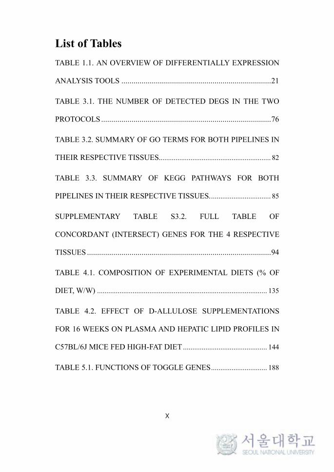
List of Tables

TABLE 1.1. AN OVERVIEW OF DIFFERENTIALLY EXPRESSION

ANALYSIS TOOLS ..........................................................................21

TABLE 3.1. THE NUMBER OF DETECTED DEGS IN THE TWO

PROTOCOLS....................................................................................76

TABLE 3.2. SUMMARY OF GO TERMS FOR BOTH PIPELINES IN

THEIR RESPECTIVE TISSUES............................................................ 82

TABLE 3.3. SUMMARY OF KEGG PATHWAYS FOR BOTH

PIPELINES IN THEIR RESPECTIVE TISSUES................................. 85

SUPPLEMENTARY TABLE S3.2. FULL TABLE OF

CONCORDANT (INTERSECT) GENES FOR THE 4 RESPECTIVE

TISSUES ...........................................................................................94

TABLE 4.1. COMPOSITION OF EXPERIMENTAL DIETS (% OF

DIET, W/W) ........................................................................................... 135

TABLE 4.2. EFFECT OF D-ALLULOSE SUPPLEMENTATIONS

FOR 16 WEEKS ON PLASMA AND HEPATIC LIPID PROFILES IN

C57BL/6J MICE FED HIGH-FAT DIET ............................................. 144

TABLE 5.1. FUNCTIONS OF TOGGLE GENES.............................. 188

XI

List of Figures

FIGURE 2.1. PAIR-CSP PLOT WITH GSE27567 DATA.................... 39

FIGURE 2.2. PAIR-DSP PLOT WITH GSE27567 DATA ................... 40

FIGURE 2.3. MULTI-RC PLOT WITH GSE27567 DATA.................. 41

FIGURE 2.4. PAIR-CSP PLOT WITH WTCCC SNP DATA............... 42

FIGURE 2.5. PAIR-DSP PLOT WITH WTCCC SNP DATA .............. 43

FIGURE 2.6. MULTI-RC PLOT WITH WTCCC SNP DATA............. 44

ADDITIONAL FILE 1 - FIGURE S2.1. PAIR-CSP PLOT WITH

MAQC RNA-SEQ DATA........................................................................ 57

ADDITIONAL FILE 2 - FIGURE S2.2. PAIR-DSP PLOT WITH

MAQC RNA-SEQ DATA........................................................................ 58

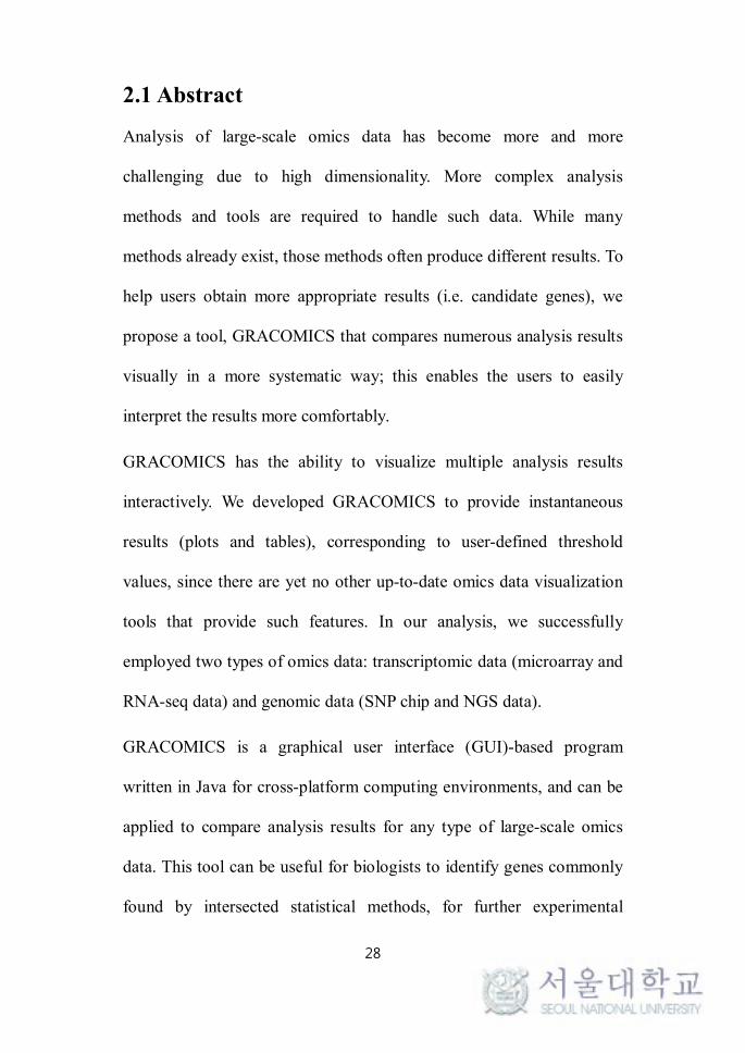
ADDITIONAL FILE 3 - FIGURE S2.3. MULTI-RC PLOT WITH

MAQC RNA-SEQ DATA........................................................................ 59

ADDITIONAL FILE 4 - FIGURE S2.4. PAIR-CSP PLOT WITH

SIMULATED NGS DATA ...................................................................... 60

ADDITIONAL FILE 5 - FIGURE S2.5. PAIR-DSP PLOT WITH


XII

ADDITIONAL FILE 6 - FIGURE S2.6. THE MULTI-RC PLOT WITH


FIGURE 3.1. FC-FC PLOT OF 4 TISSUES.......................................... 79

FIGURE 3.2. DAVID GO PLOT OF RANK AND SIGNIFICANCE IN

THE PITUITARY GLAND ..................................................................... 86

FIGURE 3.3. FC-FC PLOT OF ADIPOSE TISSUE ............................. 91

SUPPLEMENTARY FIGURE S3.1. MDS PLOT AND CLUSTERS

BASED ON RAW EXPRESSION COUNTS ........................................ 92

SUPPLEMENTARY FIGURE S3.2. EXAMPLE OF A MRNA AND

LNCRNA BASED GENE ANNOTATION SHARING A LOCI IN THE

ANTISENSE STRAND, BY THE AUTHORS OF (Muret, Klopp et al.

2017) ........................................................................................................ 93

FIGURE 4.1. EFFECTS OF D-ALLULOSE SUPPLEMENTATION

FOR 16 WEEKS ON (A) BODY WEIGHTS, (B) BODY WEIGHT

GAIN, (C-D) FOOD EFFICIENCY, (E-H) ORGAN WEIGHTS, (I)

ADIPOCYTE WEIGHTS AND (J) MORPHOLOGY ........................ 116

FIGURE 4.2. EFFECTS OF D-ALLULOSE SUPPLEMENTATION

FOR 16 WEEKS ON (A-F) PLASMA AIDPOKINES AND (G)

HEPATOTOXICITY AND (I) MASSON’S TRICHROME STAINING

OF LIVER .............................................................................................. 118

XIII

FIGURE 4.3. LAVA PLOT OF NORMAL DIET GROUP VS. HIGH

FAT DIET GROUP AND THE BOX PLOT OF THE SPEARMAN

CORRELATION FOR DEG VS. ALL GENES................................... 123

FIGURE 4.4. HEATMAP OF RECOVERED GENES (RECG) IN THE

TWO TISSUES ...................................................................................... 124

FIGURE 4.5. HEATMAP OF THE TMM NORMALIZED

MICROBIOME ABUNDANCE AND THEIR WILCOXON RANK

SUM TEST RESULTS AND CORRELATION PLOT FOR THE

LACTOBACILLUS AND COPROCOCCUS-RELATED GENES ... 127

FIGURE 4.6. QRT-PCR RESULTS OF THE 20 RECG CANDIDATES.

................................................................................................................. 136

SUPPLEMENTARY FIGURE S4.1.SEQUENCING PROTOCOLS. 138

FIGURE 5.1. Q-Q PLOT OF M1 IN EPIDIDYMAL FAT SAMPLES

................................................................................................................. 152

FIGURE 5.2. Q-Q PLOT OF M2 IN ND, ALL, AND HFD

EPIDIDYMAL SAMPLES ................................................................... 153

FIGURE 5.3. Q-Q PLOT OF M1 IN LIVER SAMPLES ................... 154

FIGURE 5.4. Q-Q PLOT OF M2 IN ND, ALL, AND HFD LIVER

SAMPLES .............................................................................................. 155

XIV

FIGURE 5.5. 4-GROUP VENN DIAGRAM OF THE BODY WEIGHT

TAGS IN EPIDIDYMAL FAT .............................................................. 156

FIGURE 5.6. 4-GROUP VENN DIAGRAM OF THE BODY WEIGHT

TAGS IN LIVER.................................................................................... 157

FIGURE 5.7. EXPRESSION PATTERN PLOTS OF A DEG-TAG

GENE CANDIDATE ............................................................................. 158

1

Chapter 1. Literature Review

2

1.1 Next-generation sequencing (NGS)

1.1.1 History of sequencing technologies

Sequencing is defined as the process of decoding the nucleotide of the

DNA sequence of the genome. Even though Maxam and Gilbert

developed the first modern sequencing technology in 1977 (Maxam and

Gilbert 1977), that of Sanger (Sanger, Nicklen et al. 1977) is known as

the first generation sequencing method or conventional sequencing

method today. Sanger sequencing uses ddNTP (dideoxyribo nucleotides

triphosphate) that do not have OH in 3’ carbon of center sugar. The use

of ddNTP is for termination; the oxygen in OH residue of 3’ carbon

provides the energy that can continue the chain reaction of DNA

synthesis. However, ddNTP, which does not have 3’-OH residue makes

the chain reaction terminated. Using such termination mechanism,

fragments of DNAs with one base pair length difference are amplified,

and electrophoresis for ordering the DNA fragments is conducted. The

nucleotide of the DNA can be identified following the order of each

nucleotide. The early stage Sanger sequencing has short read length and

small throughput of data generation. In 1986, Applied Biosystems(ABI)

introduced automated DNA sequencing that uses fluorescent primer

labeled differently for each ddNTP. The different fluorescent spectrum

of each ddNTP is used in a combined electrophoresis gel, and

3

nucleotide ordering was conducted using a computer (Smith, Sanders et

al. 1986). Using such advanced method, one can conduct sequencing

more efficiently and quickly, compared to manual decoding. In 1995,

the first-generation sequencing became automated with capillary

electrophoresis.

1.1.2 The next generation sequencing (NGS)

Sanger sequencing method is widely used, and it contributed to the

many types of research especially in the bioinformatics field. However,

the cost of the first-generation sequencing is expensive, and the amount

of data generation is limited. To solve these limitations of Sanger

sequencing, new sequencing technology named “Next-Generation

Sequencing” made its debut. This technology had low cost and rapid

data generation speed compared to previous Sanger sequencing method,

and it was employed in various types of research (Metzker 2010).

Pyrosequencing is known as the first commercialized NGS technology,

and it was developed by Jonathan Rothberg (Rothberg and Leamon

2008). The core algorithm of this method is detecting the

pyrophosphate (PPi) release on nucleotide incorporation. The released

PPis are converted quantitatively to ATPs by ATP sulfurylase.

4

Generated ATP provides energy for the luciferase-mediated conversion

of luciferin to oxyluciferin. The oxyluciferin generates visible light

which can be detected by a camera; the intensity of light is positively

correlated to the amount of synthesized nucleotide. Here, same

fluorescence is used for detection signal between 4 dNTPs; therefore,

each dNTPs—A, T, G, and C—are used once at a time. Each base is

summarized in the post-sequencing step.

In pyrosequencing, DNA synthesis is conducted until the end of

homopolymer (repeats of same base sequence) at a time. The detection

of the number of synthesized bases relies on the amount of generated

signal when homopolymer elongates each run. However, the intensity

of the signal is not precisely identical to the number of elongated bases

in the real experiment because of enzyme efficiency limitation and

signal interruption. Such variation is directly related to the read length

and ultimately with different sequence length. For this reason,

pyrosequencing suffers from InDel sequencing errors frequently (in the

homopolymer region), compared to the Sanger sequencing.

Pyrosequencing can read the fragmented DNA sequence using a single

direction method, and paired-end read can be generated using the mate-

pair library. Read length is 600 base pair in average, in GS FLX system

of Roche, and it is fairly close to the read length of Sanger capillary

5

sequencing technology.

The most representative NGS platform is the Illumina sequencing

platform. The platform is represented by Hiseq, which is the most

popular and widely used sequencing platform in 2016. The core

technology of the Illumina sequencing platform is the sequencing by

synthesis (SBS), and it is based on the nucleotide called reversible

terminator. Reversible terminator blocks 3’-end for nucleotide binding,

in a similar fashion to ddNTP of Sanger sequencing. However, a

reversible terminator can recover its 3’-OH residue for elongation as

the name might suggest. A nucleotide that has blocked 3’-OH, is

incorporated into the primer sequence, and the process of DNA

synthesis is terminated. Each reversible terminator is labeled with a

fluorescence dye, and a camera can detect it. After detecting the single-

nucleotide elongation, the 3’-end recovers its OH residue. These three

steps (nucleotide incorporation, detecting fluorescence, recover 3’-OH)

comprise one cycle, which is the core sequencing algorithm of Illumina

sequencing platforms. Only one nucleotide can be detected in a single

cycle, so Illumina’s sequencing platform does not suffer from frequent

InDel type sequencing error—a common pyrosequencing problem as

aforementioned. Illumina’s sequencing platform read the fragmented

DNA sequence using single or paired-end read method and read length

6

vary (50bp to 300bp). The read length of Illumina platforms is shorter

than that of the GS FLX system (a pyrosequencer), but it is much more

cost-effective. In addition, Illumina’s sequencing platform has the best

performance, in terms of sequencing error rate, among existing NGS

platforms.

While Sanger sequencing technology is categorized as first-generation

sequencing technology, NGS technology is classified under two

categories: the second- and the third-generation. Two aforementioned

major sequencing platforms—Rosche and Illumina—are classified as

second-generation sequencing. Second-generation technology has

distinct characteristics compared to Sanger sequencing. First, the read

length of second-generation sequencing is shorter than that of Sanger

sequencing. As an example, the Sanger sequencing has a read length of

almost 1kbp, and it is much longer than that of Illumina’s Hiseq. The

second difference is in data generation throughput and time. The

second-generation sequencing generates much more output in a

dramatically shorter period of time, compared to Sanger sequencing.

For example, one Hiseq2500 device generates 20 human genome data

of 10X coverage in almost one day, and it is tens of thousands times

faster than the Sanger sequencing device. Third is the cost. Researchers

believe that sequencing the genome will cost under $100 per individual,

7

in the near future. Forth, sequencing reactions are conducted in a

smaller sized device compared to Sanger. Lastly, the error rate is higher

than Sanger sequencing method. The error rate of Illumina platform

and pyrosequencing is known as 0.26% and 1.07%, which is greater

than the Sanger’s error rate of about 0.1%.

1.1.3 Advancements and trends in sequencing technologies

The second generation NGS platforms (Illumina Hiseq and Roche GS

FLX sequencing systems) have some common limitations. First, the

detection system uses fluorescence for both. Illumina system uses

nucleotides labeled with the specific fluorescence color for each base,

while GS FLX system detects the amount of light as a signal of the

nucleotide incorporation. This type of technology must have imaging

system for detecting the signals; this is where errors can be generated

and accumulated. For example, in each cycle of Illumina sequencing,

fluorescence molecules in the cluster have to be removed for next

nucleotide incorporation. However, quite frequently, some fluorescence

molecules remain in the cluster. The unremoved fluorescence

molecules get accumulated and fluorescence signal can be confused

with the error signal. This is the reason for the lower quality scores in

8

end of the read in Illumina sequencing system. Imaging system using

camera also can be a problem for the miniaturized sequencer.

Additionally, the second generation sequencing relies on the PCR

reaction for preparing the sequencing library. However, the GC

contents—the proportion of G and C nucleotide in total nucleotides—

can affect the PCR result; this is called “PCR bias”. The whole genome

cannot be amplified monotonously, and high or low GC regions add

more difficulty in PCR amplification. Therefore, sequencing results

using the PCR-based library are inevitably biased. Finally, the error rate

of these sequencing technologies is still higher than that of the

conventional Sanger method. In order to resolve these

problems/limitations, researchers studied and developed several

sequencing platforms and technologies. Two commercialized

sequencing platforms, ion torrent from life science and RS system from

Pacific Biosystem, are representative examples.

Ion torrent (Rothberg, Hinz et al. 2011) is based on the similar pipeline

of GS FLX system which uses the byproduct of nucleotide

incorporation similar to pyrophosphate. Instead of using the

pyrophosphate, ion torrent system detects the hydrogen ion, which is

also a byproduct of nucleotide incorporation using the pH level. This is

beneficial compared to pyrosequencing since fluorescence molecule

9

and imaging device are no longer required. With these benefits,

sequencing process can be processed on a small semiconductor chip. So

the sequencing device can be efficiently and safely miniaturized. InDel

errors, the major type of error in pyrosequencing, can also be reduced

because the signal can be detected more accurately. In addition,

sequencing time is also decreased because the sequencing step is

minimized. The Ion torrent has many benefits compared to the second

generation NGS system, however, it still is based on the amplification

of DNA fragment using emulsion PCR in library construction.

Therefore, sequencing result is not GC bias-free, and DNA fragments

with high or low GC ratio cannot be decoded efficiently.

Pacbio RS system (English, Richards et al. 2012) proposed another

sequencing algorithm. It fixed the DNA polymerase in the bottom of

the well and the DNA synthesis process is conducted in that fixed point.

However, it still uses fluorescence molecules and imaging device like

second-generation sequencing, which results in the same limitations of

second-generation sequencing technologies. As a noteworthy

characteristic however, Pacbio RS system adopts single molecular

sequencing technology although it uses fluorescence system. This

means that RS system does not use DNA amplification of the DNA

fragment for library construction like other sequencing platforms

10

(Illumina, Roche, and Ion torrent). Sequencing without PCR process

has some benefits in GC bias and RNA-seq; the resulting sequence files

contain less GC biased data, it can cover more genomic regions and

transcriptome compared to other systems. RS system also generates

long read length sequencing data compared to other sequencing

platforms. Long read length provides advantage in specificity,

haplotype, and isoforms. However, even with those benefits, Pacbio RS

system has a higher error rate (approximately >15%), which is a big

problem. The method called CCS system (circular consensus

sequencing system) (Travers, Chin et al. 2010) has been developed for

complementing this weakness. Here, hairpin structured adaptor attaches

to the end of DNA fragment, and the sequencing process can be

repeatedly conducted for individual DNA fragment. DNA fragment is

sequenced at least three times, and the consensus base call can

efficiently reduce the error rate of RS system using independent

sequencing reactions for the same location.

Illumina also improved on their weak points: (1) the read length has

increased. Miseq V2, which is the most recent sequencing platform of

Illumina, produces 300bp pair-end data. By using the overlapping

library, almost 500bp of single read can be generated for metagenome

community analysis. (2) PCR-free library preparation kit provides

11

unbiased sequencing library. PCR amplification and gel electrophoresis

was used for typical sequencing library preparation for Illumina. PCR-

free Library preparation kit (Kozarewa, Ning et al. 2009) does not

conduct PCR and use magnetic bead base for DNA isolation in library

preparation protocol. Because it does not amplify DNA using PCR, the

genome coverage of sequencing in high or low GC contents region can

be increased. So biased dispersion of sequencing coverage in genomic

location is greatly reduced. This can be used to for various genomes

with high AT regions. The third is the molecule technology for long

read data generation. This technology is developed based on the

Botryllus schlosseri genome assembly research (Voskoboynik, Neff et

al. 2013). The main concept of this technology is size-specific DNA

fragment partitioning. It analyzes and conducts assembly for the

partitioned genomic region based on the index sequences. This induces

the same effect like genome size reducing, so the molecule system can

be useful for the high heterozygous genome.

Nanopore sequencing (Branton, Deamer et al. 2008) is the 3rd-

generation sequencing platform in the true sense of the word, while the

others can be considered as 2.5th-generation. It does not use

fluorescence molecules and imaging devices. It does not amplify DNA

fragments, and it conducts sequencing on a single molecule of DNA

12

fragment. The prototype device of Oxford nanopore is portable (palm

size), and it can conduct sequencing by connecting the sequencer to a

laptop computer with a USB 3.0 cable. The algorithm of the nanopore

system is similar to that of the Pacbio system. However, it identifies the

nucleotide using the electronic signal from the nanopore protein instead

of fluorescence. Even though the accuracy and the throughput of

Oxford nanopore have to be improved, this sequencing platform

foretells the blueprint of future sequencing; portable sequencer, cheaper,

higher throughput, single molecule, etc.

In conclusion, the sequencing paradigm changes rapidly. For example,

GS FLX, the first-second generation NGS system, is no longer

available in the current market. Also, generated data from different

sequencers have different error characteristics according to their

sequencing algorithms. In example, the error profile of the Pacbio

system is different from those of second-generation sequencing

platforms, almost entirely. Therefore, researchers who want to analyze

NGS data have to understand the unique characteristics and principles

of sequencing technologies to employ proper analytical tools.

1.1.4 RNA sequencing and its applications

The NGS technique is also successfully applied in other biological

13

sources especially in RNA. In the application of NGS approach for

RNA, several studies were successfully published: such as, (1)

transcript annotation based on the reference genome (Roberts, Pimentel

et al. 2011); (2) novel transcript finding including exon, isoform, and

gene (Grabherr, Haas et al. 2011); (3) synonymous and non-

synonymous variants identification (Lu, Lu et al. 2010); (4) DEG find

in given conditions (Robinson and Oshlack 2010); (5) orthologous gene

finding among the different species (Zhu, Li et al. 2014). Of many

applications, the most acclaimed research is to detect DEG in RNA

research field. Although the primary goal of the RNA-seq is to identify

RNA sequence, it is possible to quantify the target transcript by using

mapped reads count on reference genome with transcriptome

annotation (Mortazavi, Williams et al. 2008). Before the development

of RNA-seq, cDNA microarray chip was widely used in order to detect

DEG. However, since some limitations were introduced from the

comparative studies against microarray and RNA-seq (Mortazavi,

Williams et al. 2008, Wang, Gerstein et al. 2009), mRNA extraction

platform gradually switched over from microarray to RNA-seq. There

are many advantages to employing NGS based RNA study. First, the

dependency on existing knowledge is less in the RNA-seq platform. In

the microarray platform, probe design step for targeted RNA should be

14

conducted before experimenting. In order to construct probe, targeted

RNA sequence should be known. On the other hand, the RNA-seq

experiment can be directly performed without preliminary information.

While RNA annotations (Gene annotations) are well developed in

model organisms, the annotation is still not well-organized in non-

model organisms. For this reason, RNA-seq is widely used in diverse

species instead of the microarray. Second, RNA-seq is better than

microarray regarding reusability. Due to the probe designing step in

microarray generated microarray data can measure only targeted RNA.

On the contrary, RNA-seq can simultaneously measure diverse types of

RNA sequences such as mRNA, miRNA (Humphreys and Suter 2013),

lncRNA (Tilgner, Knowles et al. 2012), etc., because of

unnecessariness of the probe design. Although some RNA annotation is

insufficient in the present state, RNA-Seq data can be re-used anytime

when the statement of annotation is improved enough to apply real data

analysis. Finally, RNA-seq provides highly reproducible gene

expression measures (Marioni, Mason et al. 2008, Mortazavi, Williams

et al. 2008). In the microarray platform, there are several problems

related to the technical biases including dye effect and several batch

effects (Churchill 2002). In short, hybridization step mainly causes

technical biases in the microarray. On the other hand, RNA-seq is less

15

technical biased than microarray because hybridization is unnecessary.

From these advantages, today in 2015, a large number of studies

perform identification of transcriptomic features related to diverse

conditions on several species. More detailed reviews about these

transcriptome analysis are included in Chapter 1.2.

16

1.2 Transcriptome data analysis

1.2.1 Reference genome-based approach

The RNA-seq analysis pipeline can be divided into majorly two

groups: (1) reference genome-based and (2) de novo assembly-based

approaches. However, this thesis is focused on the reference genome-

based approach on model organisms that do not require de novo

assembly. Most of RNA-seq analyses include re-sequencing step based

on the well-constructed reference genome and transcriptome annotation.

In this case, the model-species such as human, mouse, and arabidopsis

with reliable background knowledge are often used; the reference

genomes of model species are generally in high quality (sequencing

generated in high depth coverages and validated). Therefore, if the

reference genome is available, the re-sequencing approach is preferable.

The reference genome-based approach often includes four steps as

shown in Figure 1.1-a. First, reads are generated from the RNA samples

and filtered for adapter sequences, which would cause inaccurate result

in downstream analysis. In addition, reads of poor quality is also

filtered out as they could lead to complications in RNA-seq experiment.

Some computational methods were developed for generating clean

reads (Lindgreen 2012). Among various methods, Trimmomatic

17

(Bolger, Lohse et al. 2014) is widely used in the first step of RNA-seq

experiment using Illumina’s platform. In the next step, reads are

aligned to the appropriate position of the reference genome. The widely

used aligners include; BWA (Li and Durbin 2009), Bowtie2 (Langmead

and Salzberg 2012), ELAND (Bentley, Balasubramanian et al. 2008),

TopHat (Trapnell, Pachter et al. 2009), GSNAP (Nookaew, Papini et al.

2012), and etc. While some studies compared performance of various

aligners, (Grant, Farkas et al. 2011) concluded that it is impossible to

determine the best aligners considering all conditions because mapping

rate is profoundly affected by many factors (i.e. genome structure).

Therefore, employing and comparing several aligners is recommended.

Subsequently, the next step is the quantification step (Trapnell, Roberts

et al. 2012, Anders, Pyl et al. 2014). In this step, the number of reads

mapped on each feature (exon, gene, isoform or etc) of the reference

genome is counted based on transcriptome annotation. Finally,

statistical analysis is performed using the raw-counts. Generally, the

computational methods can be classified into two groups, but both of

the groups use similar statistical methods. More detailed literature

reviews for RNA-seq analysis in the statistical perspective is included

in Chapter 1.2.2.

1.2.2 Statistical analysis for RNA-seq data

18

The computational methods (Garber, Grabherr et al. 2011) and

statistical methods (Rapaport, Khanin et al. 2013, Soneson and

Delorenzi 2013) were developed along with the advance of the RNA-

seq platform. In the statistical view, the RNA-seq analysis can be

divided into two different topics: normalization and testing. In case of

normalization, main purpose is to accurately measure relative gene

expression by adjusting for systematic biases, such as gene length,

library size, GC-contents, and etc (Robinson and Oshlack 2010). The

statistical methods proposed to tackle these problems include: (1) reads

per kilobase of exon model per million mapped reads (RPKM)

(Mortazavi, Williams et al. 2008); (2) guanine-cytosine content (GC-

content) normalization (Risso, Schwartz et al. 2011); (3) Quantile

normalization (Hansen, Irizarry et al. 2012); (4) trimmed mean of M-

values (TMM). RPKM was introduced to consider gene length when

measuring relative gene expressions. By doing this, the different

possibility of read mapping to longer or shorter genes can be

normalized. In addition, some studies have reported that GC-content

could influence gene expression, which could result in false positives in

downstream analysis (Hansen, Irizarry et al. 2012). In another report, a

method of GC-content normalization was suggested (Risso, Schwartz et

al. 2011). Quantile normalization, based on the rank of the gene

19

expression, has been widely used in microarray which is helpful for

controlling batch effects. Finally, TMM normalization is the most

commonly used method for determining relative expression of genes.

In case of the other normalizations, experimental design cannot be

considered when calculating relative gene expressions. However, RNA-

seq experiment is generally performed under the given conditions for

detecting DEGs. In the transcriptome analysis, one of the basic

assumptions is that most genes are not differentially expressed in any

conditions. TMM normalized values and normalized factors are

calculated based on this idea, using whole gene expression and library

sizes in each sample (Robinson and Oshlack 2010). In addition,

calculated normalized factors can be used in generalized linear model

(GLM) as additional offsets.

RNA-seq and microarray analysis are different in several ways when

viewed from statistical perspective. One of the differences is usage of

GLM in RNA-seq analysis for detecting DEGs. To perform statistical

analysis, several assumptions on the distribution of gene expression are

needed. Several controversies exist in distribution of gene expression

derived from RNA-seq experiment. It can be assumed that the relative

gene expression derived from microarray follows normal distribution.

Under this circumstance, well-established statistical methods such as t-

20

test, ordinary regression, and analysis of variance (ANOVA), can be

used for the test corresponding to the experimental design (Forster, Roy

et al. 2003, Sreekumar and Jose 2008). On the other hand, integer count

can be observed in RNA-seq (abundances is observed as count), similar

to serial analysis of gene expression (SAGE). Several statistical models

were well-established for considering count-type distribution as in

SAGE (Vêncio, Brentani et al. 2004, Robinson and Smyth 2008).

Based on these models, edgeR was developed (Robinson, McCarthy et

al. 2010). The distribution of the mapped-counts was considered as

over-dispersed Poisson model (negative binomial distribution) with

using empirical Bayes method to estimate degree of overdispersion in

the genes. In general, Poisson distribution can be assumed to model the

mapped count. However, Poisson-model-based approaches failed due to

the overdispersion problem (Auer and Doerge 2011, Fang and Cui

2011). For this reason, recent studies use negative-binomial distribution.

Under this assumption, many statistical methods such as edgeR, DESeq

(Anders and Huber 2012) and DESeq2 (Love, Huber et al. 2014) were

developed which use GLM, considering mapped-count as response

variable. The model can easily be extended to complex design by

including additional factors. Generally, the transcriptome is highly

sensitive to variables compared to the genomic sequence, therefore

21

controlling for these variables is important. Uncontrolled factors can be

adjusted using GLM and this is the reason why GLM is widely used in

RNA-seq analysis. With the reduction of the cost associated with RNA-

seq experiment, RNA-seq experiment with more complicated design

will become a feasible option and hence the importance of GLM-based

RNA-seq analysis is expected in the future.

22

Table 1.1. An overview of differentially expression analysis toolsNormalization,

Quantitative analysis and Differential

Expression tools

EdgeR DESeq DESeq2 limmavoom

Balllgown

cuffdiff2 EBSeq baySeq PoissonSeq

NOIseq SAMseq

Quantification measure

Count-based

Count-based

Count-based

Count-based, linear model

Linear model

Count-based

Count-based,Linear model

Count-based

Count-based

Count-based

Count-based

Normalization TMM/Upper quartile/

RLE (DESeq-

like)/None (all scaling factors are set to be

one)

Median-of-ratio

Median-of-ratio

TMM FPKM Geometric(DESeq-

like)/quartile/classic-fpkm

Median Normalizat

ion

Scaling factors

(quantile/TMM/total)

Total count of least

differental genes

(assessed by GOF)

RPKM/TMM/Upper quartile

Poisson Sampling

Read count distribution assumption

Negative binomial

distribution

Negative binomial

distribution,

Poisson distribution (no or few replicates)

Negative binomial

distribution

Negative binomial

distribution

Beta negative binomial

distribution

Negative binomial

distribution

Negative binomial

distribution

Negative binomial

distribution

Negative binomial

distribution

Nonparametric

method, empirical

distribution (no or few replicates)

Nonparametric

method

Differential expression test

Exact test Exact test Exact test Empirical Bayes

method

Parametric F-test

comparing nested linear

models

t-test Evaluates the

posterior probability

of differentially and non-differential

ly expressed

entities (genes or isoforms)

via empirical Bayesian methods

Assesses the

posterior probabilities of models

for differentially and non-differential

ly expressed genes via empirical Bayesian methods and then compares

these posterior

likelihoods

Score statistic on the basis of

the a Poisson

log limear model

Contrasts fold

changes and

absolute differences

within a condition

to determine the null

distribution and then compares

the observed

differences to this null

Wilcoxon rank

statistic and a

resampling strategy

23

Support for multi-factored experiments

Yes Yes Yes Yes Yes No No No Yes Yes Yes

True positive rate High Low Low/Medium

Low/Medium

Medium/High

Low Independent of

sample size

Low High Not clear Low(small sample sizes)/

High(large enough sample sizes)

Support differential

express detection without

replicated samples

Yes Yes No No No Yes No No Yes Yes No

Detection of differential

isoforms

No No No No Yes Yes Yes No No No No

Runtime for experiments

Minutes Minutes Minutes Minutes Seconds(standard laptop)

Hours Hours Hours Seconds highly dependent on sample

size

highly dependent on sample

size

24

1.3 Biomarker selection

1.3.1 Statistical thresholds

In statistics, use of p-values from test statistics quickly became more

conventional compared to simple comparison of means. Traditional

biological literature have used fold-change, of the means, as the

differential expression threshold. While summarizing multiple values to

a single mean or average loses variance information, test statistics such

as t-test, considers the variance of all values in each group. In multi-

group comparisons, the mean and variance of group 1 is compared to

that of another via ANOVA or t-test under normality assumptions.

While nonparametric tests can be use on small datasets, linear models

with normality assumptions were frequently used by bioinformaticians

in microarray analysis and in FPKM or RPKM-based RNA-seq

analyses, along with the threshold of p-value < 0.05.

The p-values in big datasets such as NGS or microarray data, however,

had to be adjusted for multiple testing problem; the GWAS studies with

hundred-thousands of SNPs had to be analyzed, and the increase in

number of tests results in an increase in error. The simplest method is

Bonferroni correction, which is followed by the false discovery rate

(FDR) (Benjamini and Hochberg 1995). The Bonferroni correction

25

multiplies the raw p-values by the number of genes tested from the

dataset. The FDR divides the Bonferroni corrected p-values by their

raw p-value rank, which leads to more power over Bonferroni. While

various methods have been proposed to correct multiple testing

problem, the two aforementioned methods are the only ones accepted

by researchers at a consensus level. Even after the RNA-seq paradigm

has shifted from FPKM and RPKM to raw gene expression counts with

Poisson and negative binomial assumptions, p-values and multiple

testing threshold still hold their grounds in suggesting plausible

candidates.

1.3.2 Biomarker Presentation

In presentation of candidate genes, traditional scatter plots, Venn

diagrams, box plots are frequently used in bioinformatics. More and

more people alter basic plots to highlight and emphasize their findings.

In pre-2003, while the resolution of microarray results were not up to

today’s level, findings from microarray analyses could not be trusted,

and had to be validated. And for technical validation, certain threshold

of mean difference had to exist to detect DEGs. Here, the fold-change

made its return to bioinformatics, and has been used as a

complimentary threshold to p-values. In 2003, the Volcano plot made

its debut (Cui and Churchill 2003), which is a plot that comprise x-axis

26

with fold-change between groups and y-axis with –log(p-value,10). Up-

and down-regulation information is shown by the x-axis, and fold-

change threshold could be added as vertical lines. The p-value of each

gene are plotted according to the fold-change, and is usually color-

coded based on the horizontal threshold of adjusted or raw p-values.

27

This chapter was published in BMC Genomics (2015) 16:256

as a partial fulfillment of Joon Yoon’s Ph.D program

Chapter 2. GRACOMICS: Software for GRaphical

COMparison of multiple results with omics data

28

2.1 Abstract

Analysis of large-scale omics data has become more and more

challenging due to high dimensionality. More complex analysis

methods and tools are required to handle such data. While many

methods already exist, those methods often produce different results. To

help users obtain more appropriate results (i.e. candidate genes), we

propose a tool, GRACOMICS that compares numerous analysis results

visually in a more systematic way; this enables the users to easily

interpret the results more comfortably.

GRACOMICS has the ability to visualize multiple analysis results

interactively. We developed GRACOMICS to provide instantaneous

results (plots and tables), corresponding to user-defined threshold

values, since there are yet no other up-to-date omics data visualization

tools that provide such features. In our analysis, we successfully

employed two types of omics data: transcriptomic data (microarray and

RNA-seq data) and genomic data (SNP chip and NGS data).

GRACOMICS is a graphical user interface (GUI)-based program

written in Java for cross-platform computing environments, and can be

applied to compare analysis results for any type of large-scale omics

data. This tool can be useful for biologists to identify genes commonly

found by intersected statistical methods, for further experimental

29

validation.

Keywords

GUI, microarray, NGS, omics, RNA-seq, SNP, visualization

30

2.2 Introduction

Over the last decade, success in microarray data studies has led to an

expansion of large-scale omics data analyses and their data types. Vast

amounts of data, in various forms, are produced for a common goal: to

find genetic variants related to a phenotype of interest (e.g., disease

status, etc.). In unison with technological advances, many statistical

tools were developed for separate types of omics data analyses. In our

study, we will illustrate the application of our tool for different omics

data types.

Many microarrays studies aim to detect “gene expression signatures”

specific to various human diseases by comparing expression levels

between two distinct groups. The main idea is to identify overexpressed

and underexpressed genes, as compared to a control group, and label

them as deleterious or protective, respectively. The success of this

approach in human cancer, and other diseases (Pan 2002), promoted the

development of many statistical methods. However, unifying the

analysis results from disjointed methods cannot keep up with the

explosive rate of publications concerning the specific phenotype of

interest. Thus, annotation and replication studies are required in this

current era. Many databases, such as the National Center for

Biotechnology Information (NCBI), have been used to infer biological

31

information from omics data and make note of novel findings that were

detected as previously reported “markers.”

The popularity of another type of array-based study, focusing on

single nucleotide polymorphism (SNP) association studies, has steadily

increased. In fact, SNP analysis has been crucial in uncovering the

genetic correlations of genomic variants with quantitative traits,

complex diseases, and drug responses (Hirschhorn and Daly 2005).

One well-known data source, the Welcome Trust Case Control

Consortium (WTCCC) database, which handles 14,000 cases of seven

common diseases and 3,000 shared controls, has led to many influential

publications. While various analysis methods have been published, and

public databases such as dbSNP (Sherry, Ward et al. 2001) and

HapMap (Gibbs, Belmont et al. 2003) are available, utilizing them well

is another issue.

Following the footsteps of array-based approaches, an era of high-

throughput sequencing began, and this technology has been applied to

RNA-seq and whole exome and genome sequencing. RNA-seq has

properties that are different from microarrays, for example, a high

dynamic range and low background expression levels. To address these

properties, several statistical methods using Poisson or negative

binomial distributions have been proposed (Vitale, Frabetti et al. 2007,

32

Huang, Sherman et al. 2009, Choi, Lee et al. 2014). In the case of

exome and genome sequencing, issues with missing heritability have

led researchers to study more than just common variants, and various

methods have now been proposed to handle rarer variants (Troyanskaya,

Garber et al. 2002, Nagato, Kobayashi et al. 2005, PATANI, JIANG et

al. 2008).

As for visualization tools, there are only a few programs available

for comparison. Multi Experiment Viewer (MeV) (Howe, Holton et al.

2010) is one of the most popular tools included in the TM4 suite, which

is used to analyze microarray data. Although it supports several

statistical methods of microarray data analysis, MeV provides only

multiple outputs in treeview. Similar to MeV, PLINK (Purcell, Neale et

al. 2007) is a widely used genome association analysis toolset, but does

not provide graphical interactive comparison of results.

Here, we focused on exploring the inconsistent results that can be

produced from method-specific assumptions and parameters. Taking an

extra step to check, understand, and interpret the different results can be

challenging for scientists without computational proficiency. We aimed

to ease such problems by proposing a visual comparison tool in a user-

friendly environment. In addition to its accessibility, GRACOMICS can

reflect a change in results according to an immediate alteration of

33

significance levels. Such characteristics are valuable, and likely

essential for effective, interactive, and integrative comparison of

multiple results. Therefore, the proposed tool, GRACOMICS, provides

a novel approach to visually compare several test results through

graphical user interface (GUI) components.

In addition to its interactive GUI, our tool provides three distinctive

layouts for comparison, including pairwise plots, summary tables, and a

“heatmap-like” summary table highlighting pivotal markers, commonly

detected by different methods. Two of the modules, the Pairwise

Comprehensive Scatter Plots Module (Pair-CSP) and the Pairwise

Detailed Scatter Plot Module (Pair-DSP), compare and contrast a pair

of methods at the same time, while the third, the Multiple Results

Comparison Module (Multi-RC), can handle all the employed

methods (more than two) at once. Note that the user can define the top

N significant markers (from input files) that will be used in the modules,

for more interactive and efficient comparison. Furthermore, simple

web-annotation functionality adds to the benefits, in terms of biological

interpretation.

2.3 Materials and Methods

2.3.1 Microarray dataset and statistical methods

34

For microarray studies, statistical tests were performed to detect

differentially expressed genes (DEGs) between two groups: cases and

controls. A pre-processing step is necessary for statistical analysis of

the raw expression profiles, including background correction, global or

local normalization, log-transformation, etc. Such processing steps may

alter the results and should be performed only after fully understanding

the platform and target probes of the analysis. We employed a

microarray dataset, GSE27567 (LaBreche, Nevins et al. 2011), from the

Gene Expression Omnibus (GEO) database, consisting of 45,101

Affymetrix probes from 93 individual mice. To detect the DEGs from

the microarray data, we perform two group comparison tests between

tumor-bearing mice and non-transgenic controls. We employed

statistical tests such as t-test, significant analysis of microarray (SAM)

(Tusher, Tibshirani et al. 2001), permutation, and Wilcoxon rank-sum

test.

2.3.2 SNP dataset and statistical methods

In genome-wide association (GWA) studies, researchers focus on the

positions of genetic variants that are significantly related to the

phenotype of interest. There is no gold standard for pre-processing such

data, but a few guidelines exist. Many steps, such as normalization and

35

bias removal are included in data pre-processing, and the analysis

results are very dependent on those steps. In our analysis, we used a

bipolar disorder data in the WTCCC database, which includes 354,019

SNPs from 4,806 individuals (1,868 bipolar disorder patients and 2,938

normal controls). As a first step, we conducted a quality control process

based on specific criteria (Oh, Lee et al. 2012). For the association test

between genotype and phenotype, using SNP data, we used statistical

methods such as chi-square test, Fisher’s exact test, logistic regression

with covariate adjusting, and logistic regression without covariate

adjusting. These association tests were implemented using the PLINK

tool (Purcell, Neale et al. 2007).

2.3.3 RNA-seq dataset and statistical methods

We employed results from RNA-seq, another type of transcriptome

measuring platform. Recently, its advantages over microarray

platforms have been described by many comparative reports

(Morozova, Hirst et al. 2009). Thus, a more elaborated estimation

became possible by RNA-seq, in short. However, RNA-seq gene

expression is measured in counts (i.e., number of strands synthesized),

and therefore direct application of RNA-seq methods to microarray

analysis is impossible. Instead, RNA-seq analysis methods are

36

developed by applying statistical methodologies based on analyzing

serial analysis of gene expression (SAGE) platform data, a traditional

approach for measuring gene expression in counts. Here, we employed

RNA-seq data from a previous study (Bullard, Purdom et al. 2010)

using edgeR (Robinson, McCarthy et al. 2010), DESeq (Anders and

Huber 2010), and NBPSeq (Di, Schafer et al. 2011) methods. The

RNA-seq data from a MicroArray Quality Control Project (MAQC)

had 7 replicates and one pooled sample each from two types of samples,

Ambion’s (Austin, TX, USA) human brain reference RNA, and

Stratagene’s (Santa Clara, CA, USA) human universal reference RNA.

After filtering out the NA values; 10,473 genes remained, with three

DE-analysis methods.

2.3.4 NGS dataset and statistical methods

Shortcomings of common variants in explaining the whole heritability

of diseases has led to the study of rarer variants (Troyanskaya, Garber

et al. 2002, Nagato, Kobayashi et al. 2005, PATANI, JIANG et al.

2008). Unlike common variants, rare variant analyses, based on single

genetic associations, often shows large false-negative results, unless the

sample or effect sizes are very large. Hence, collapsed genotype scores

for a set of rare variants are suggested for an analysis scheme. For our

37

input, we employed the results from rare variant association tests such

as C-alpha (Neale, Rivas et al. 2011), burden test (Wu, Lee et al. 2011),

and SKAT-O (Lee, Emond et al. 2012). These association tests were

implemented using the FARVAT tool (Choi, Lee et al. 2014). For

illustrative purposes, we used the simulation dataset of FARVAT

consisting of 100 SNPs and 16 genes which was enlarged to have

10,000 SNPs and 2,000 genes, using the same settings.

2.3.5 Implementation of GRACOMICS

GRACOMICS is a java-based stand-alone program using a GUI

platform. It was developed under Java because statistical analysis tools

are generally developed by diverse codes such as R, SAS, etc. Java

programs are renowned for their compatibility with various computing

environments, are supported by all operating systems, and can easily be

executed by other programs written in different computer languages.

GRACOMICS can read tabular types of tab-separated values (TSV)

files containing p-values for each method in columns and genetic

markers in rows. Also, using simple mouse clicks, rather than command

lines as input, helps bridge the gap between biology-based researchers

and computer science-based researchers. Our plan was to design and

implement a user-friendly program any researcher could use in any

38

environment. The proposed tool, GRACOMICS, has the following

three interactive modules with distinct features:

(1) Pairwise Comprehensive Scatter Plots Module (Pair-CSP)

Pair-CSP provides a scatter plot of pairwise comparisons between

statistical method inputs simultaneously (Figures 2.1 and 2.4). Pair-CSP

automatically generates these pairwise scatterplots using the p-values

from the input file(s), letting the user interpret the similarities between

the test results through correlation plots and correlation coefficients at a

glance. When the significance level is manipulated, the pairwise

scatterplots change accordingly, to display markers over the threshold

only. There are two reasons behind this feature: one is to reduce

computational time for drawing multitudinous points, and the other is

to show only what the researcher wants to see, i.e., the meaningful

results.

(2) Pairwise Detailed Scatter Plot Module (Pair-DSP)

Pair-DSP is an interactive plot to compare the results between two

methods on a more detailed level than Pair-CSP (Figures 2.2 and 2.5).

This module is linked to Pair-CSP, enabling the user to directly access

Pair-DSP from Pair-CSP for extended summarization of the chosen

biomarkers. The summary organizes meaningful results via a Venn

diagram, a table, and a marker list. For the known marker’s function,

39

simple annotation of a single biomarker is offered via the NCBI

database. Its simple annotation function automatically provides a link

to the NCBI web page corresponding to its marker type, for

convenience. In addition, for pathway analysis of microarray data,

GRACOMICS connects to the web-based DAVID database (Huang,

Sherman et al. 2009). As a result, researchers can summarize their list

of significant results, and then check the biological functions of the

chosen markers.

(3) Multiple Results Comparison Module (Multi-RC)

Multi-RC provides simultaneous comparison of numerous test results

(Figures 2.3 and 2.6). Researchers can choose an interesting subset of

methods and set their significance levels separately. A tabular output

with rows as significant markers and columns as statistical methods, is

provided (with p-values in each cell). Each cell is color-coded red or

green, representing significant or not, respectively. Also, variation of

color intensities are used to represent the degree of significance, with

more significant markers colored more intensely. In addition, Multi-RC

summarizes commonly significant results and provide links to their

annotation. As an extra option (with a checkbox) for meta-studies, we

implemented Fisher’s method in combining p-values to provide overall

importance in version 1.1.

41

Figure 2.1. Pair-CSP plot with GSE27567 data.

Four test results were compared, and all pairwise scatterplots and their correlation coefficients are given in the Pair-CSP module.

42

Figure 2.2. Pair-DSP plot with GSE27567 data.

Wilcoxon rank sum tests and t-tests were chosen for detailed investigation, Venn diagram and the summary tables are key features of Pair-DSP.

43

Figure 2.3. Multi-RC plot with GSE27567 data.

The Multi-RC module provides an overall summary in a heatmap-like tabular format which highlights markers with the lowest average p-values. The user can then choose which methods to investigate by using the checkboxes in the top-left panel.

44

Figure 2.4. Pair-CSP plot with WTCCC SNP data.

Four tests results were compared, and all pairwise scatterplots and their correlation coefficients are given in Pair-CSP.

45

Figure 2.5. Pair-DSP plot with WTCCC SNP data.

Two logistic models, one with and the other without covariates, has been chosen for detailed investigation, Venn diagrams and the summary tables are key features of Pair-DSP.

46

Figure 2.6. Multi-RC plot with WTCCC SNP data.

The Multi-RC module provides an overall summary in a heatmap-like tabular format which highlights markers with the lowest average p-values. Note rs1112069 is colored in red by 3 of the 4 tests, as discussed in the manuscript.

47

2.3.6 Availability and requirements

Project name: GRACOMICS (License: LGPL 2.1)

Project home page: http://bibs.snu.ac.kr/software/GRACOMICS

Operating system: Platform-independent

Programming language: Java

Other requirements: Java 1.7.0_45 or higher

2.3.7 List of abbreviations

SNP: Single nucleotide polymorphism

GUI: Graphic User Interface

NCBI: National Center for Biotechnology Information

WTCCC: Wellcome Trust Case Control Consortium

Mev: Multi Experiment Viewer

Pair-CSP: Pairwise Comprehensive Scatter Plots Module

Pair-DSP: Pairwise Detailed Scatter Plot Module

Multi-RC: Multiple Results Comparison Module

DEGs: differentially expressed genes

GEO: Gene Expression omnibus

SAM: significant analysis of microarray

48

GWA: genome-wide association

TSV: tab separated values TSV

SAGE: serial analysis of gene expression

MAQC: MicroArray Quaility Control Project

49

2.4 Results and Discussion

2.4.1 Results

Application of GRACOMICS to real microarray data

In Figure 2.1, the plots provided by Pair-CSP compare the test results

of t-test, Wilcoxon rank-sum test, SAM, and permutation test,

displaying the top 1,500 markers by their average p-values (the user

can designate the number or percentage of markers to be displayed).

Pair-CSP reveals a close relationship between each pair of methods;

most correlation coefficients are over 0.9, except for those with the

Wilcoxon rank-sum test. Although both Wilcoxon rank-sum and

permutation tests are nonparametric tests, the Wilcoxon rank-sum test

uses only rank information, while the permutation test uses the variance

information that arises when defining t-test statistics. Thus, they

provide different results.

In order to compare the Wilcoxon rank-sum test to other tests more

systematically, we used Pair-DSP focusing on the t-test and the

Wilcoxon rank-sum test. As shown in Figure 2.2, Pair-DSP displays a

pairwise plot of the two methods using p-values, and summarizes the

number of genes commonly identified by the two methods. Unlike the

pairwise plot of Pair-CSP, the pairwise plot of Pair-DSP shows far more

detailed information. For example, a red color represents the significant

50

genes identified by t-test only, a blue color signifies those identified by

Wilcoxon rank-sum test only, and purple color indicates those

identified by both tests. The gene name, in tool tip form, of a point is

provided when the cursor is put directly over the single point. The

summary table, at the top right, shows a decrease in the number of

significant genes commonly identified by the two methods goes from

1,049 to 12, as the cut-off value decreases from 5% to 0.1%. Pair-DSP

also provides a Venn diagram displaying the numbers of genes

identified commonly and separately by the two methods. Pair-DSP

shows that 171 genes remained significant by both t-tests and Wilcoxon

rank-sum tests at the 1% significance level. 86 genes were significant

by t-test only and 141 genes by Wilcoxon rank-sum test only, at the

same significance level. The bottom right table shows the list of genes

identified by the two methods.

To investigate the functions of the identified genes, simple

annotation is provided via the NCBI database. This simple annotation

function automatically opens a link to the NCBI web page

corresponding to the gene of interest, for convenience. In addition, for a

pathway analysis annotation database, GRACOMICS provides

connection to the web-based DAVID database (Huang, Sherman et al.

2009). For example, clicking the gene Cyyr1, followed by a right click

51

shows a popup window with two menus of “Link to NCBI annotation

database” and “Link to DAVID annotation database”. From the NCBI

database, researchers can investigate known gene functions, and related

papers in PubMed, for each gene. We observed that Cyyr1 (Vitale,

Frabetti et al. 2007) and Il9 (Nagato, Kobayashi et al. 2005) are genes

reported in PubMed. Next, when using DAVID to analyze the

functional annotation of the 171 commonly identified genes from t-tests

and Wilcoxon rank-sum tests, we observed the gene list to be enriched

in the GO term “cell cycle arrest,” with a p-value of 4.1e-3. As a result,

researchers can summarize their list of significant results, and then

check the biological functions and related publications of the chosen

markers.

The Multi-RC module allows simultaneous comparison of two or

more results, as shown in Figure 2.3. We selected four methods: t-test,

SAM, Wilcoxon rank-sum test, and permutation test, with a cut-off

value of 0.1%. In this setting, we observed 12 common significant

genes between all the methods. The genes BB471471, Cyyr1, Il9, and

St6galnac1 (PATANI, JIANG et al. 2008) were consistent candidates

from all four methods. However, while BB471471 was at the top of the

list, no reports were found of its association with tumours or any other

diseases. Therefore, we suggest the BB471471 is a worthy candidate to

52

examine further for its possible association with tumours. By analyzing

this real microarray data analysis with GRACOMICS, we identified

several commonly significant DEGs from comparisons from each

method, to obtain the most reliable candidate DEGs.

Application of GRACOMICS to real SNP data

In Figure 2.4, the plots are provided by Pair-CSP, which compares the

test results of chi-square test, Fisher’s exact test, and logistic regression

analyses. In the figure, two results from logistic regression analyses are

provided: one is without covariates and the other is with the adjusting

covariate effects of sex, age and the first two principal components.

Although the significance of covariates can be easily tested, it is not

always straightforward to determine which adjusting covariates to

include in the model (Troyanskaya, Garber et al. 2002). Here, we

focused on the results from the two logistic models and demonstrate

how efficiently GRACOMICS can be used to compare these two results,

showing that the correlation between the two logistic regression models

was 0.598.

For a further detailed comparison between these two results, Pair-

DSP, in Figure 2.5, was conducted on these two logistic models. The

summary table, at the top right, shows that the number of significant

genes commonly identified by the two methods gradually decreases

53

from 15 to 4, as the cut-off value decreases from 5.0e-6 to 2.4e-6. The

Venn diagram illustrates that Pair-DSP successfully identified

rs1344484 (Palo 2010), rs708647, rs2192859 (Kwon, Park et al. 2014),

rs11647459 and rs4627791(Jiang and Zhang 2011), in purple, as the

most commonly detected SNPs. The four SNPs in red, rs11112069,

rs1375144, rs11622475, and rs4627791, were detected by the with-

covariates model only. We found rs11112069 as the top result (in

average p-value), with low p-values in all four analyses. This SNP is

within intron-2 of CHST11, a gene which has previously been reported

as bipolar disorder-associated (Chen, Lu et al. 2014).

In the next module (Multi-RC; Figure 2.6), users can see the change

in p-values for each marker, according to the method used or

adjustments for covariates. Rs11112069 is displayed at the top of the

list, and is marked in red (very significant) from 3 of the 4 tests, with a

fairly low p-value for the fourth test also. To further analyze the top

results, GRACOMICS can automatically distinguish marker types and

links to dbSNP in the NCBI database for selected SNPs. From the

annotation, researchers can attain detailed SNP information, such as

location of the SNP, its mapped gene, clinical significance, etc. Unlike

the microarray example, DAVID is not directly applicable to SNP data.

However, we expect that other annotation databases will be added to

54

future updates.

Application of GRACOMICS to real RNA-seq data

As shown in Figure S2.1, Pair-CSP shows that all three analysis

methods; edgeR, DESeq, and NBPSeq, yield very similar results. All of

the correlation coefficients are over 0.86, and the highest was between

edgeR and DESeq. In addition, the plots illustrate that edgeR generates

lower P-values than the others, due to scattered points being skewed

toward the y-axis (edgeR). Under the 1% significance level,

approximately 7,000 genes were detected as DEGs by each method. In

Figure S2.2, Pair-DSP shows that more DEGs were identified by edgeR,

as compared to DESeq. In the Venn diagram, significant genes that

intersected ranged from 7087 to 1621, when decreasing the cut-off

values from 0.01 to 1.0E-100. Finally, we can observe that most of

genes are very significant in Multi-RC. As shown in Figure S2.3, 6983

genes were detected by all the methods under a 1% significant level.

Here, the gene symbol of RNA-seq data is its Ensemble ID, and these

should be converted to official gene symbols for successful functional

annotation. Although implementing the Ensemble annotation function

on the web is possible, we did not include it in the current version of

GRACOMICS, because accommodating several symbols in the

program may lead to user confusion. Although we determined that only

55

official gene symbols should be accommodated in the tool, later

versions can be updated with such functions, if there are user demands.

Application of GRACOMICS to simulated NGS data

Using a simulated rare variant dataset (Choi, Lee et al. 2014), we

successfully cataloged significant genes that were test-specific or

marginal in all tests. The results are shown in Figures S2.4~S2.6. In this

analysis, gene names were masked as Genes 1 ~ 2000 and therefore

could not be annotated to NCBI or DAVID. However, if a real dataset is

used, the genes can be annotated in similar fashion as microarray and

RNA-seq datasets. In accord with the above three applications, we

could infer which methods showed higher correlation, in terms of p-

values, from the Pair-CSP, followed by a detailed comparison of the

number of significant genes detected in each method, and finally, by

comparing the p-values in a tabular heatmap form. Here, we observed

the highest correlation of 0.961 between the C-Alpha and SKAT-O

methods, and these two methods shared 129 genes with a p-value

threshold of < 0.05. The top-ranked genes all showed p-values ~ 0.001

using all the methods, and would be candidates of interest for end-users

if this was a real data analysis.

2.4.2 Discussion

From the aforesaid illustration, we demonstrated the potential of

56

GRACOMICS to successfully highlight biologically meaningful results

from multiple methods. Traditional bioinformatics studies, and some

recent works, show that simple comparison of results has been widely

used for biological interpretation. For example, a transcriptome study

concluded that in a situation where the most reliable list of markers is

desirable, the best approach was to examine the intersection of genes

identified by all tried methods, or by more conservative tests

(Troyanskaya, Garber et al. 2002). Since checking the underlying

assumptions of all methods is not easy, and even if the assumptions are

met, each method may provide different results, which are hard to

interpret. The easiest and most conventional method is to find

commonly identified markers to trim down the candidate list, and carry

on further analysis. While GRACOMICS cannot give conclusive

evidence that the highlighted markers are significant, it can help the

biologist narrow down the candidate list, based on the intersection of

markers for efficiency for further validations, such as RT-PCR.

In addition to comparison of multiple results of the same datasets,

GRACOMICS can be applicable to other types of studies. First,

GRACOMICS can compare the results from different datasets, such as

different tissues or organs. An RNA study compared differentially

expressed test results from various tissues, such as liver, adipose tissue,

57

muscle, and brain (Jiang and Zhang 2011). GRACOMICS can

effectively provide the list of common genes, as well as tissue-specific

genes. Second, GRACOMICS can compare results from different

platforms, such as microarray vs. RNA-seq (Nookaew, Papini et al.

2012). Here, GRACOMICS can trim down the list of candidates

significant to both platform results, for further biological validation.

Finally, meta-analysis combining independent results from different

studies can be analyzed by GRACOMICS; the p-values from each

study can be efficiently compared to others and can be combined easily

by Fisher’s method. For meta-analysis, the compared results should be

from independent datasets. However, when one single dataset was

analyzed by multiple methods, the independent assumption is violated;

the interpretation of this Fisher’s combined p-value should be made

with caution.

2.4.3 Conclusion

Comparative study of omics data analyses is unavoidable; however,

many researchers skip the comparative step because it is a complicated

process. GRACOMICS enables easy comparison of several methods

for analyzing specific omics data platforms by any user. The four omics

data employed are active areas of study in bioinformatics. We

employed microarray & RNA-seq data at the transcriptomic level, and

58

SNP and NGS data at the genomic level, to display the utility of

GRACOMICS. So far, GRACOMICS can also employ proteomic

analysis results, and will be extended to accommodate other types of

annotations for proteomics data in a future study. In summary, we

believe that this will be a highly valuable and straightforward tool for

non-computational biologists, strongly assisting them in their

interpretation of results from new cutting-edge technologies.

59

Additional file 1 - Figure S2.1. Pair-CSP plot with MAQC RNA-seq

data.

Three tests results have been compared, and all pairwise scatterplots and their correlation coefficients are given on Pair-CSP.

60

Additional file 2 - Figure S2.2. Pair-DSP plot with MAQC RNA-seq

data.

EdgeR and DESeq were chosen for detailed investigation. Venn diagrams and the summary tables are key features of Pair-DSP.

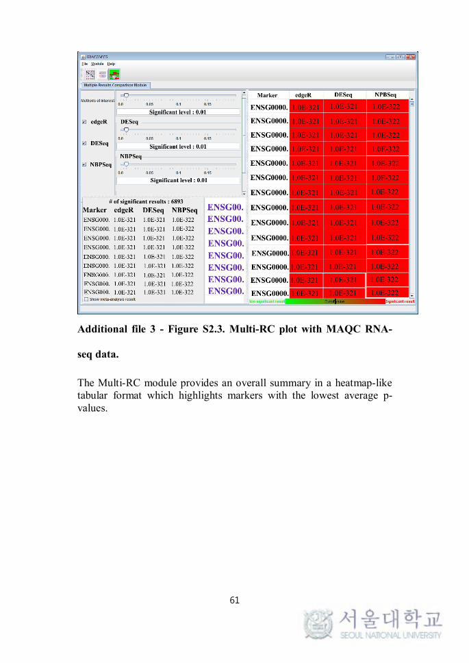
61

Additional file 3 - Figure S2.3. Multi-RC plot with MAQC RNA-

seq data.

The Multi-RC module provides an overall summary in a heatmap-like tabular format which highlights markers with the lowest average p-values.

62

Additional file 4 - Figure S2.4. Pair-CSP plot with simulated NGS

data.

Three tests results were compared, and all pairwise scatterplots and their correlation coefficients are given on the Pair-CSP GUI.

63

Additional file 5 - Figure S2.5. Pair-DSP plot with simulated NGS

data.

C-alpha and SKAT-O were chosen for detailed investigation. Venn diagrams and the summary tables are key features of Pair-DSP.

64

Additional file 6 - Figure S2.6. The Multi-RC plot with simulated

NGS data.

The Multi-RC module provides an overall summary in a heatmap-like tabular format which highlights markers with the lowest average p-values.

65

This chapter will be published in Asian-Australasian Journal of Animal

Sciences as a partial fulfillment of Joon Yoon’s Ph.D program

Chapter 3. Multi-tissue Observation of the Long Non-coding RNA Effects on Sexually Biased Gene

Expression in Cattle

66

3.1 Abstract

Recent studies have implied that gene expression has high tissue-

specificity, and therefore it is essential to investigate gene expression in

a variety of tissues when performing the transcriptomic analysis. In

addition, the gradual increase of lncRNA annotation database increased

the importance and proportion of mapped reads accordingly. We

employed simple statistical models to detect the sexually

biased/dimorphic genes and their conjugate lncRNAs in 40 RNA-seq

samples across two factors: sex and tissue.

We employed simple statistical models to detect the sexually

biased/dimorphic genes and their conjugate lncRNAs in 40 RNA-seq

samples across two factors: sex and tissue. We employed two

quantification pipeline: mRNA annotation only and mRNA+lncRNA

annotation.

As a result, the tissue-specific sexually dimorphic genes are affected by

the addition of lncRNA annotation at a non-negligible level. In addition,

many lncRNAs are expressed in a more tissue-specific fashion and with

greater variation between tissues compared to protein-coding genes.

Due to the genic region lncRNAs, the differentially expressed gene list

changes, which results in certain sexually biased genes to become

ambiguous across the tissues.

67

In a past study, it has been reported that tissue-specific patterns can be

seen throughout the differentially expressed genes between sexes in

cattle. Using the same dataset, this study used a more recent reference,

and the addition of conjugate lncRNA information, which revealed

alterations of DEG lists that result in an apparent distinction in the

downstream analysis and interpretation. We firmly believe such

misquantification of genic lncRNAs can be vital in both future and past

studies.

Keywords: Cattle, Sexually dimorphic, Genic lncRNA, RNA-seq,

Expression profile, Tissue specificity

68

3.2 Introduction

Recent studies have shown the importance of long non-coding RNA

(lncRNA) annotation is growing with time. Their quantified expression

levels are at a fair level and therefore needs additional handling if a

study handles transcriptome. In recent literature (Derrien, Johnson et al.

2012), the simple definition of a lncRNA is written as non-coding

RNAs that are long, stable, commonly spliced, and polyadenylated,

plus transcribed from their own promoters. Also, in (Zhang, Yang et al.

2014), the author states that most large intergenic non-coding RNAs

(lincRNAs) appear indistinguishable from mRNAs, due to the 5' cap

structures and 3' poly(A) tails. Such characteristics should arouse a

question in a scientist’s mind if the mRNA expression really from a

mRNA. Furthermore, we have to be sure that our mRNA expression

level is trustworthy, in order to detect differential gene expression. By

adding the lncRNA annotation and accounting for their counts, one can

remove ambiguous reads that were originally quantified as mRNA in

traditional approaches.

Our understanding of the molecular mechanisms underlying sexual

dimorphism remains imperfect. A common practice in the

transcriptomic analysis is to attesting the gene expression between

groups of population and treatments. While many of dimorphism

69

studies are published for humans, rodents, and fruit flies, only a few

were attempted in cattle (Chitwood, Rincon et al. 2013, Gómez,

Caamaño et al. 2013). To add, most bovine transcriptomic research

focuses on the tissue growth and development, which are exclusive

studies on pre-implantation embryos. Other tissues should also be taken

into account for further insight into these mechanisms.

Bovine meat and milk are everyday sources of human nutrition (Mwai,

Hanotte et al. 2015). The gender and gender-specific genes of the food-

producing animal are known to affect the quality and quantity of those

nutrients (Splan, Cundiff et al. 1998, Gill, Bishop et al. 2009).

Investigation of sexual dimorphism in metabolic tissues such as muscle,

liver and adipose tissue from cattle is important for both research and

the food production industry. Previous works have already proven the

gender- and tissue-specific effects in expression profiles (Yang, Schadt

et al. 2006). The between-gender expression should be compared in

every tissue that is available.

While the entire brain is filled with sexually dimorphic (or biased)

features, the hypothalamus-pituitary axis is a primary structure that

controls sexual dimorphism in the central nervous system (CNS), as

well as peripheral tissues. The pituitary gland regulates the central

endocrine of metabolism, sexual maturation, and growth. Its unique cell

70

types in the anterior secrete polypeptide hormones such as growth

hormone and gonadotropins, a family of protein hormones including

luteinizing hormones and follicle stimulating hormones, by

appropriately orchestrating signals from environmental and internal

stimuli. Furthermore, profound sex differences exist in hormonal

regulation and responses of the pituitary gland to external stressors,

which leads to the females displaying a higher vulnerability to various

neuropsychiatric disorders (Handa, Burgess et al. 1994, Rhodes and

Rubin 1999). Hence, examination of sexually dimorphic gene

expression profiles in the pituitary gland in multiple metabolic tissues

will improve our understanding of sexual dimorphism in both

metabolic and physiological perspectives (Nishida, Yoshioka et al.

2005, Sanchez-Cardenas, Fontanaud et al. 2010).

In the present study, we aimed to revisit the tissue-specific sexually

dimorphic genes that contribute to bovine sexual dimorphism.

Generalized linear model is utilized for analyzing complex RNA-seq

data from samples collected from several different tissues- liver, muscle,

visceral adipose tissue and pituitary gland: a simple two-group

comparison for detecting sexually dimorphic genes in each tissue. We

followed two pipelines—mRNA annotation only and mRNA with

lncRNA annotation—and we report the differences in these approaches

71

for identification of sexually dimorphic genes in several tissues. While

a few of the recent studies published results of mRNA and lncRNA

profiling in RNA-seq, none were written on revisiting the old datasets

and how the list of DEGs differentiates from the original manuscripts

(Seo, Caetano-Anolles et al. 2016).


3.3.1 Animal handling and RNA-seq procedures

The dataset is open in public from previous literature (Seo, Caetano-

Anolles et al. 2016). However, in their preprocessing of the dataset, the

outdated protocol such as reference file, annotation file, alignment and

quantification programs have been updated with a more concurrent in-

house pipeline. As a note, the sex-chromosome annotation is discarded

due to its absence in bostau8 reference (the most concurrent bovine

reference file). The detailed Animal handling and RNA-seq procedures

are provided in the Supplementary File 1 as an excerpt from their

original manuscript, as no extra handling or processing of animals and

RNA samples were done.

Here, the mRNA pipeline (original) only considers mRNA-to-gene

annotation, while our pipeline includes the lncRNA annotation

additional to that of the mRNA in the quantification step. After

preprocessing of the data, Hisat2 (Kim, Langmead et al. 2015) and

72

featureCounts (Liao, Smyth et al. 2014) (non-stranded) have been

employed to acquire the counts of our features. Hisat2 and

featureCounts are a pair of the most concurrent genome-based

quantification tools that are compatible with those from the previous

study (since validations will be cited). In the process, the General

Transfer Format (GTF) file from UCSC genome browser has been used,

and the lncRNA annotation GTF from ALDB (A Domestic-Animal

Long Noncoding RNA Database) (Li, Zhang et al. 2015) has been

utilized. To account for the lncRNAs, we merged the two GTFs were

merged as one and quantified with featureCounts. As a result, we

achieved 19212, 19823, 19144, 19918, and 19208, 19817, 19139,

19913 genes respectively in the 4 tissues (Liver, Fat, Muscle, and

Pituitary Gland) for mRNA and mRNA + lncRNA pipelines. Default

options were used except for the unstranded option for both programs.

There were a few contaminated and ambiguous samples that had low

mapping and annotation rates; such samples are highlighted in the

Supplementary Table 3.1, and are removed from the analysis for quality

control purposes.

3.3.2 Statistical model for detecting sexually dimorphic genes in

each tissue using GLM implemented in edgeR

73

In a previous study, various sexually dimorphic genes were detected

by two group tests in four tissues using the same data (Seo, Caetano-

Anolles et al. 2016). The study considered a count-type distribution

such as Poisson and negative binomial (one solution for over-dispersion

in Poisson assumption), which is suitable for measuring gene

expression from RNA-seq data given data characteristics. Hence, GLM

is employed for analysis of RNA-seq data by assuming gene expression

as a negative binomial in edgeR to detect DEGs. However, the study

used an outdated source, reference (bostau7 and annotation), while we

have updated those sources (bostau8 and annotation) and added

lncRNA information in our protocol.

We chose the simpler model for identification of sexually dimorphic

genes using RNA-seq data composed of two factors (sex and tissues).

The simplest approach for the analysis of this data is to perform a two-

group test between data from female and males in each tissue,

separately, as has been performed in previous studies using microarray

data. To extend this method in RNA-seq analysis, we employed a

generalized linear model (GLM) with only one explanatory variable

(sex group variable) as shown.

log(E(Y))=μ+Sex

The reason behind this is that the tissue specificity is obvious when

74

using the MDS to cluster our expression profiles which shows much

higher between-tissue variance than between-individual or –group, as

shown in Supplementary Figure S3.1. In other words, the tissue has

more effect on the expression level than sex or individual, which is

concordant with the previous work (Seo, Caetano-Anolles et al. 2016).

When a full model considering the sex and tissue is fitted, the

interaction term is significant for a major part of the considered genes;

this also means that the sexually dimorphic genes should be separately

attested for each tissue. In other words, a simple analysis of deviance

(ANODEV) model is more adequate compared to a reduced two-factor

model, which includes tissue as a covariate, when the interaction term

between sex and tissue is significant, and that effect of sex on gene

expression changes with the tissue. Since lncRNA expression is also

known for its tissue-specificity (Iwakiri, Terai et al. 2017), we carried

out the analysis using the tissue-specific simple ANODEV model. The

ANODEV model is a GLM that is frequently used in RNA-seq studies

by considering the dependent variable as a Poisson distribution; it is a

GLM compatible version of analysis of variance analysis (ANOVA)

(Nelder 2006). We used an FDR < 0.05 significance cutoff for multiple

testing adjustments and summarized the significant genes for each

tissue separately.

75

3.3.3 Availability of supporting data

The public datasets supporting the results of this article is available in

the GEO database, GSE65125 in

http://www.ncbi.nlm.nih.gov/geo/query/acc.cgi?acc=GSE65125.

3.3.4 List of Abbreviations

ANODEV: Analysis of deviance

CNS: Central nervous system

DEGs: Differentially expressed genes

FDR: False Discovery Rate

GLM: Generalized linear model

GTF: General Transfer Format

lncRNA: long non-coding RNA

qRT-PCR: Quantitative real-time PCR

3.3.5 Supplementary file excerpt

Excerpt from (Seo, Caetano-Anolles et al. 2016) on Animal handling

and RNA-seq procedures as we used the published dataset and refined

76

the study. [These are direct quotes from the article, and should be

removed from the manuscript while checking for plagiarism.]

“All animal procedures were approved by the National Institute of

Animal Science Institutional Animal Use and Care Committee

(NIASIAUCC), Republic of Korea, and performed in accordance with

the animal experimental guidelines provided by NIASIAUCC. Samples

were collected from Korean cattle raised in the Daekwanryung

experimental branches of the National Institute of Animal Science

(NIAS). 10 cattle were slaughtered at age of (>22 months) and carcass

weight was 353 ± 36 kg after slaughter. Abdominal adipose tissue, liver,

intact longissimus dorsi muscle, and pituitary gland tissue samples

were immediately separated after slaughter. Tissue samples were stored

at -80 °C, and total RNA was isolated from the four tissues using the

TRIzol reagent (Invitrogen) based on the manufacturer instructions.

Total RNA quality and quantity was verified using a NanoDrop1000

spectrophotometer (Thermo Scientific, Wilmington, DE, USA) and

Bioanalyzer 2100 (Agilent technologies,Palo Alto CA, USA). The

mRNA in total RNA was converted into a library of template molecules

suitable for subsequent cluster generation using the reagents provided

in the Illumina ® TruSeq™ RNA Sample Preparation Kit. In summary,

mRNA was purified using poly-A selection, then chemically

77

fragmented and converted into single-stranded cDNA using random

hexamer priming. The second strand is then generated to create double-

stranded cDNA that is ready for TruSeq library construction. The short

ds-cDNA fragments were then connected with sequencing adapters, and

suitable fragments were separated by agarose gel electrophoresis.

Finally, truseq RNA libraries were built by PCR amplification,

quantified using qPCR according to the qPCR Quantification Protocol

Guide, qualified using the Agilent Technologies 2100 Bioanalyzer.

(Agilent technologies,Palo Alto CA, USA). Based on the generated

RNA libraries, paired-end sequencing (101 bp read-length and

approximately 150 to 180 insert size) was performed using the HiSeq™

2000 platform (Illumina,San Diego, USA). Next, to measure

transcriptome levels with generated RNA-seq reads we performed the

following widely used RNA-seq pipeline: (1) We employed

Trimmomatic (v0.32) (Bolger, Lohse et al. 2014) with following option:

PE -phred33 ILLUMINACLIP:TruSeq3-PE.fa:2:30:10 MINLEN:75 2

for making clean reads.”


3.4.1 Results

Identification of sexually dimorphic genes using the one-way model

in each tissue

78

By using our simple ANODEV model, we identified differentially

expressed genes for each pipeline and summarized their results by

finding the intersecting genes (concordant genes) and pipeline-specific

genes. In the original pipeline, mRNA only annotation, there were 37,

23, 40, and 31 genes significant for muscle, adipose tissue, pituitary

gland, and liver, respectively. For our pipeline, with mRNA and

lncRNA annotation, 38, 23, 40, and 31 genes were respectively

detected. Although the numbers may seem similar, as in pituitary gland,

the proportion of intersecting gene is not significant when considering

all tissues. Specifically, out of the 23 significant genes, only 3 genes are

significant in adipose tissue expression. Other tissues also display a

sufficient number of pipeline-specific DEGs as shown in (Table 3.1):

Table 3.1. The number of detected DEGs in the two protocols.

Type* Muscle Adipose

Tissue

Pituitary

Gland

Liver

Intersect 17 3 33 23

mRNA only 20 20 7 8

mRNA &

lncRNA

21 20 7 8

*The three types in the table are intersection DEG between the two pipelines and each

pipeline-specific DEGs.

80

One can easily observe the different composition of DEGs that results

from the addition of lncRNA annotation and their tissues. In the

(Additional Figures 3.1-8) of the supplementary of the online version,

the top 10 genes of each analysis are illustrated with between-sex

boxplots; different gene and rank composition can be seen from the

figures, yet, we focus on the downstream analyses of the full DEG lists.

Identification of sexually dimorphic genes in relation to sex

biasedness.

Sex biasedness is usually defined by the over-expression in one or the

other sex. Hence, the upregulated genes in the female samples can be

defined as female-biased, and the genes down-regulated in the female

samples can be defined as male-biased in our analysis (the males are

used as controls). In the following plot, the first quadrant contains

genes that are female-biased in both protocols, the third quadrant

contains those biased for males, and the second and fourth quadrants

contain ambiguous genes that change regulation direction by the

inclusion of lncRNA annotation.

Figure 3.1, is a union of the significant results between the two

pipelines, for each tissue; in other words, the figure displays the DEGs

from mRNA pipeline and mRNA+lncRNA pipeline combined. The

81

grey nodes are the intersection genes, DEGs from the mRNA only

pipeline are color-coded with blue, while the DEGs from our pipeline

(mRNA & lncRNA) are coded in red. One can observe the intersection

genes have similar Fold-changes, and the pipeline-specific genes have

significant differences between the fold-change of expression.

Therefore, we provide separate lists of DEG for the concordant

(intersect) and discordant (mRNA only- or mRNA & lncRNA-specific)

genes for the different tissues. The grey genes, which are concordantly

significant between the two pipelines, are the most stable and

unaffected by the inclusion of lncRNA. We suggest these genes to be

carried on to technical validation, for their consistency. Genes such as

CYP7A1 and EPYC are included in the intersect list and has been

validated with qRT-PCR in the previous study (Seo, Caetano-Anolles et

al. 2016) to be sexually dimorphic in both cattle and rat species. The

full list of concordant genes is provided in the (Supplementary Table

S3.2). Of course, a comprehensive validation is more appropriate, yet a

partial validation of a list implies sex biasedness on the rest of the

genes in the list when further technical validation is impossible. To add,

the newly detected DEGs in the second pipeline illustrates that

checking the DEG list in common practice with our suggested pipeline

is vital.

83

Figure 3.1. FC-FC plot of 4 tissues.The fold-change in the mRNA pipeline is in the x-axis and fold-change in the suggested pipeline is in the y-axis. The plot displays the difference in fold-changes between the same BAM files under different quantification pipeline. The intersecting genes (grey; black border), and pipeline-specific genes (blue and red) are respectively color-coded.

84

Downstream GO term and KEGG pathway analysis

We analyzed our DEG sets with DAVID (Wei Huang and Lempicki

2008) for GO term and KEGG pathway analysis. Newly appearing and

disappearing list of GO terms and KEGG pathways are identified in

Tables 3.2 and 3, respectively.

According to Tables 3.2 and 3.3, for the muscle, pancreatic secretion

pathway (bta04972) and BP term of anterior/posterior pattern

specification (BP_GO:0009952) are uniquely found for the mRNA only

pipeline. In contrast, cholesterol metabolic process (BP_GO:0008203)

and chromosome segregation (BP_GO:0007059) is found in our new

pipeline. In adipose tissue, motor activity (MF_GO:0003774) and

cytoplasm (CC_GO:0005737) are respectively found unique for mRNA

only and our pipeline. As for the liver, retinol metabolism (bta00830)

and chemical carcinogenesis (bta05204) disappears from the list as the

lncRNA is added to the gene list. As bolded and italicized in Table 3.3,

an interesting term that has been removed by the addition of lncRNA in

the pituitary gland is the ‘nicotine addiction.’ Those genes were mostly

down-regulated in the female samples in comparison to males.

Additionally, long-term synaptic potentiation (BP_GO:0060291) is

found unique for the original pipeline, and serine-type peptidase

85

activity (MF_GO0008236) is found unique for the new pipeline, as

shown in Figure 3.2. The serine-type peptidase activity has been

reported as a sex-biased gene in previous literature (Immonen, Sayadi

et al. 2017).

86

Table 3.2. Summary of GO terms for both pipelines in their respective tissues.

TissuePipeline

8Term

Coun

tPValue

Fold

Enrichmen

t

P.

GlandmRNA

GO:0016998~cell wall

macromolecule catabolic

process

53.69E-

08135

P.

GlandmRNA

GO:0050829~defense response

to Gram-negative bacterium5

1.61E-

0655.38462

P.

GlandmRNA GO:0019835~cytolysis 4

9.66E-

0690.94737

P.

GlandmRNA


to Gram-positive bacterium5

1.05E-

0534.83871

P.

GlandmRNA

GO:0007417~central nervous

system development3

0.00473

728.17391

P.

GlandmRNA GO:0007155~cell adhesion 4

0.00669

49.988439

P.

GlandmRNA GO:0007586~digestion 2

0.05674

933.23077

P.

GlandmRNA

GO:0060291~long-term

synaptic potentiation2

0.05886

832

P.

GlandmRNA

GO:0021766~hippocampus

development2

0.07148

726.18182

P.

GlandmRNA

GO:0005615~extracellular

space14

1.20E-

087.120197

P.

GlandmRNA

GO:0005578~proteinaceous

extracellular matrix4

0.00540

510.79679

87

P.

GlandmRNA GO:0003796~lysozyme activity 6

2.25E-

10154.0588

P.

GlandmRNA

GO:0005540~hyaluronic acid

binding2

0.04552

541.57143

P.

GlandmRNA


matrix structural constituent2 0.07886 23.59459

Adipos

emRNA GO:0003774~motor activity 2

0.02984

659.52273

Muscle mRNAGO:0009952~anterior/posterio

r pattern specification2

0.04882

236.42688

P.

Gland

mRNA+

lncRNA

GO:0016998~cell wall

macromolecule catabolic

process

52.79E-

08144

P.

Gland

mRNA+

lncRNA


to Gram-negative bacterium5

1.22E-

0659.07692

P.

Gland

mRNA+

lncRNAGO:0019835~cytolysis 4

7.86E-

0697.01053

P.

Gland

mRNA+

lncRNA


to Gram-positive bacterium5

8.01E-

0637.16129

P.

Gland

mRNA+

lncRNA

GO:0007417~central nervous

system development3

0.00415

430.05217

P.

Gland

mRNA+

lncRNAGO:0007155~cell adhesion 4

0.00554

210.65434

P.

Gland

mRNA+

lncRNAGO:0007586~digestion 2

0.05318

335.44615

P.

Gland

mRNA+

lncRNA

GO:0021766~hippocampus

development2

0.06702

827.92727

P. mRNA+ GO:0005615~extracellular 12 1.21E- 6.103026

88

Gland lncRNA space 06

P.

Gland

mRNA+

lncRNA

GO:0005578~proteinaceous

extracellular matrix4

0.00540

510.79679

P.

Gland

mRNA+

lncRNAGO:0003796~lysozyme activity 6

2.25E-

10154.0588

P.

Gland

mRNA+

lncRNA

GO:0008236~serine-type

peptidase activity2

0.03701

151.35294

P.

Gland

mRNA+

lncRNA

GO:0005540~hyaluronic acid

binding2

0.04552

541.57143

P.

Gland

mRNA+

lncRNA


matrix structural constituent2 0.07886 23.59459

Adipos

e

mRNA+

lncRNAGO:0005737~cytoplasm 6

0.02000

12.983789

MusclemRNA+

lncRNA

GO:0008203~cholesterol

metabolic process2

0.05975

731.27602

MusclemRNA+

lncRNA

GO:0007059~chromosome

segregation2

0.08001

723.11706

* The two pipelines are separated by a double-line break. The pipeline specific terms and their specific values are bolded if there are differences

between the two pipelines’ result.

89

Table 3.3. Summary of KEGG pathways for both pipelines in their respective tissues.

Tissue Pipeline* Term Count PValueFold

Enrichment

P. Gland mRNAbta04970:Salivary

secretion3 0.006106 22.84036

P. Gland mRNAbta05033:Nicotine

addiction2 0.059304 30.09127

Liver mRNAbta00140:Steroid

hormone biosynthesis3 0.002403 36.2823

Liver mRNAbta00830:Retinol

metabolism2 0.072718 24.1882

Liver mRNAbta05204:Chemical

carcinogenesis2 0.08862 19.6961

Muscle mRNAbta04972:Pancreatic

secretion2 0.049696 31.59583

P. GlandmRNA+

lncRNA

bta04970:Salivary

secretion3 0.008538 19.57745

LivermRNA+

lncRNA

bta00140:Steroid

hormone biosynthesis2 0.058602 29.56335

*The two pipelines are separated by a double-line break. The pipeline specific terms and their specific values are bolded if there are differences between the

two pipelines’ result.

124

Differential gene expression in relation to anti-obesity and anti-

inflammation

In our DEG analysis, the three groups were cross-analyzed in two

tissues: liver and epididymal fat. The significant DEGs between ND vs.

HFD, ND vs. ALL, and HFD vs. ALL were summarized, functionally

annotated, and classified for their roles in the biological pathways. In

the one-way models of the liver, 1) ND vs. HFD produced 3,892 (up:

2298, down: 1594), 2) ND vs. ALL produced 1,202 (up: 551, down:

651), and 3) HFD vs. ALL produced 2,625 (up: 766, down: 1859)

DEGs (FDR adjusted p-value < 0.05). As for the epididymal fat, 1) ND

vs. HFD produced 1,915 (up: 1442, down: 473), 2) ND vs. ALL

produced 606 (up: 262, down: 344), and 3) HFD vs. ALL produced

2,394 (up: 315, down: 2079) DEGs. Further interpretation on the

within-tissue intersecting genes of those analyses are as follows:

A. 1) and 2) intersecting genes contains genes that did not recover from

HFD effect even with the allulose intake (directions match) or that

allulose intake overshoots the recovery (directions discordant).

B. 1) and 3) intersecting genes contains genes that are ameliorated by

allulose intake—recovery gene (RecG)—(if the regulation direction is

discordant, intake of allulose results in an ND-like expression of the

125

genes in ALL group), and genes that are not related to obesity or

inflammation (concordant directions)

C. 2) and 3) intersecting genes contains three types; partial recovery for

the discordant regulation, and non-related genes or overshooting genes

for the concordant regulation direction.

In the liver, the A genes comprise 644 matching and 19 discordant.

Similarly, the B genes comprise 36 and 1566, and the C genes are 194

non-related, 152 overshooting, and 129 partial recovered genes were

observed. As for the epididymal fat, respectively 353, 5, 0, 874, 27, 68,

and 46 genes were observed. The discordant genes of list B (liver and

epididymal; 1566 and 874) are important for crosstalk evaluation in the

following chapters.

Crosstalk gene detection

According to the lava plot, the significant DEGs displayed a higher

between-group DE correlation in the two tissues, compared to the full

expression profile (Figure 4.3a, 4.3b). This means that the significant

gene’s expression in one tissue has some interaction with the same

gene’s expression in the other tissue; hence, the definition of cross-talk.

We could observe there may be a correlation between the crosstalk

genes in terms of Fold changes also.

126

By using a boxplot, we compared the Spearman correlation between the

log2-transformed fold changes between the two tissues in two different

datasets: Full data and significant gene set (Figure 4.3c). In

concordance with the lava plot, the significant genes displayed the

much higher correlation between Fold changes compared to that of the

whole dataset.

In addition to the lava plot and box plot, we illustrated the between-

tissue crosstalk with TMM normalized expression of our analyses

(Figure 4.4). To show the expression profile of the RecGs, TMM

expression of 4 one-way models—ND vs. HFD and HFD vs. ALL, in

two tissues—were employed. Since the TMM normalization is applied

to ND-HFD samples and HFD-ALL samples differently, the two HFD

values are both incorporated in the plot. There is no surprise that the

range of expression is different between the two tissues. However, the

expression profile of the significant genes showed a similar pattern

across the tissues; there is some clear distinction between HFD versus

ALL samples, which may not be as significant against ND, yet the

proof of gene expression regulation of allulose on HFD samples is

clearly present. Generally, the ALL samples show much similar

expression with the ND compared to that of HFD in the profile. The

heatmap is a direct in silico validation of the RecG, which are candidate

127

genes that are regulated by allulose to a normal diet-like level. From the

selected RecGs, we further narrowed down the candidates with log2

fold-change > 1 and intersected in the two lists to retrieve 60 crosstalk

RecGs. The fold-change threshold ensures enough between-group

difference to be easily detected in technical validation (i.e. qRT-PCR)

of the 60 genes. The tissue-specific p-values of the ND versus HFD and

HFD versus ALL, sub-category, and gene function is summarized

(Table 4.3). The sub-categories are color-coded by each gene’s relation

to Cancer, Cell division, inflammation, immune system, and Others.

128

Figure 4.3. Lava plot of normal diet group vs. high fat diet group and the

box plot of the Spearman correlation for DEG vs. all genes.

The significant genes are color-coded based on the combined p-value (Fisher’s method) of the two tissue-specific test p-values. The X-axis is the log2 fold change of the Liver analysis, while the Y-axis is the log2 fold change of the Epididymal analysis. For the detection of crosstalk genes, the genes have to be concordantly significant, in terms of FDR-adjusted p-value, and have marginal log2 fold change > 1. Hence, the vertical lines (blue and red) are log2 fold change cutoffs for Epididymal DEGs, and similarly, the horizontal lines (blue and red) are cutoffs for the Liver DEGs. To illustrate the correlation between significant DEGs and the two tissue-specific p-values, a) significant DEGs and b) all genes are plotted. As for the boxplot c), all three models—HFDvsALL, NDvsALL, and NDvsHFD—are represented by red, blue, and green-like colors, respectively. The darker colors are the correlation value of all

genes, while the lighter colors are for the significant genes.

129

Figure 4.4. Heatmap of recovered genes (RecG) in the two tissues.

The group indicators represent the HFD_1 from ALLvsHFD, HFD_3 from NDvsHFD, ALL, and ND group. The 4 groups on the left are from the liver analysis, and the other 4 are from the epididymal analysis. Scaled colors are TMM normalized gene expression of each groups, and as the ALL and ND groups and the two HFD groups

are similar, they are paired with each other in the heatmap.

130

Microbiome analysis in relation to anti-obesity and anti-inflammation

In SCFAs analysis, D-allulose supplementation was significant

decreased in acetate concentration and concentration of propionate and

butyrate was shown to increase tendency. The two Genera—

Lactobacillus and Coprococcus—of the Firmicutes were highlighted as

inflammation-related genus (Figure 4.5a). The Wilcoxon rank sum test

has been used to test the differential abundance between the groups (P

<0.05). The ALL group has a significant increase in Lactobacillus and

Coprococcus genus composition compared to the other two groups. To

investigate the RecGs that are correlated with the microbiota that are

representative for anti-inflammation, we calculated the correlation

(Spearman) between microbiome abundance of the two aforementioned

genera and gene expression profiles of the RecGs (Supplementary table

4.2). In addition, to link both tissues with the abundance of the two

genera, we focused on the crosstalk genes that have negative

correlation in both tissues. This is due to the fact that 59 of the RecGs

are overexpressed in HFD samples compared to ND and ALL. As a

result, we discovered 20 genes with Gm12250 as the most correlated

gene. From the aforementioned 5 sub-categories, the majority of the

final 20 genes are inflammation-related suggesting the strong

relationship between inflammation and the two genera of interest.

132

Figure 4.5. Heatmap of the TMM normalized microbiome abundance and their Wilcoxon Rank Sum test results and Correlation plot for the Lactobacillus and Coprococcus-related genes.

The production of (A) acetate (CH3COOH), (B) propionate (CH3CH2COOH) and (C) butyrate (C4H8O2), representative SCFAs, was shown in figure 43 in feces. Acetate production was increased by ALL group compared to HFD group, however, propionate and butyrate productions had increasing tendency compared to HFD group.(D) The microbiome abundance is color-scaled based on their TMM-normalized abundance. Group Indicators are above and the phylum information is given to the right of the microbiome heatmap. Statistical test between group is given by the Wilcoxon rankSum columns; the green is for up-regulation and red is for down-regulation. Each column of the tests are the results for NDvsALL, NDvsHFD, and HFDvsALL. The asterisk (*) on the test names represent the control samples. (E) The correlogram of the twenty most correlated genes to the inflammation-related Firmicutes, Lactobacillus and Coprococcus, in two tissues are illustrated. The negative to positive correlation is color-coded with blue and yellow. The left two columns are for liver, and the other two are for eWAT. Accordingly, “_L” is for liver and “_E” is for eWAT.

133

4.4.2 Discussion

134

A positive energy imbalance excess energy intake, decreased energy

expenditure, and cause obesity, which leads to metabolic complications

and chronic inflammation. Many studies suggest that D-allulose has

beneficial effects against obesity and diabetes in mice (Hossain,

Kitagaki et al. 2011, Han, Han et al. 2016, Shintani, Yamada et al.

2017). However, its underlying molecular mechanisms in chronic

inflammation caused by obesity remain unclear. In past study, D-

allulose improved the diet-induced obesity by regulation of the mRNA

expressions in small intestine, liver and eWAT (Shintani, Yamada et al.

2017). This study demonstrated molecular mechanisms of metabolic

regulation in response to D-allulose supplementation in diet-induced

obese C57BL/6J mice under pair-fed condition, based on the

transcriptomic analysis of mRNA-seq and microbiome.

WAT is an active endocrine organ, which secretes adipokines including

cytokines, chemokines, and hormones as well for storing energy (Jung

and Choi 2014). Appropriate adipokine secretion exerts an effect on

energy homeostasis, glucose and lipid metabolism in normal status.

However, obesity and HFD feeding promotes inflammatory cytokines

secretion and decreased anti-inflammatory adipokines from WAT.

In our study, HFD feeding in mice, plasma interleukin 1-β, interleukin

6, TNF-α, interferon-»and resistin levels were elevated, but D-allulose

135

supplement lowered those plasma levels together with reduction of

body weight and body fat mass. In RecGs, CCl2, Clec7a, Gm12250,

Itgax, Trem2 and UBD, which promotes inflammatory cytokines

secretion, were down regulated in eWAT and liver due to D-allulose

supplementation.

It is a well-known fact that gene expression profiles differ among

tissues, and such difference can be hazardous in statistical models with

tissue as a main factor. In a two-way model without interaction term,

the assumption is that the gene expression slope between the two are

the same, which can be proven by the insignificance of the interaction

term in the full model. We have checked the two-way models and their

interaction terms; the majority of the interaction terms in the models

were significant, suggesting a split data analysis between tissues. As a

safest measure, considering the tissue-specificity, we used simple

ANODEV models in each tissue to select the genes affected by D-

allulose supplementation. Then, we filtered out less-informative

candidates, and trimmed down the crosstalk gene list of interest by

removing discordant regulation between tissues. A narrower definition

of crosstalk—concordant expression regulation—shows more direct

interaction between the tissues. However, the discordant regulation may

also provide insight into the between-tissue communication where up-

136

regulation in a tissue may cause down-regulation in the other, vice

versa. In terms of gene expression pattern/profile between tissues, DEG

candidates displayed much higher correlation; the spearman correlation

between fold change in liver versus that of the epididymal fat of the

significant genes are well above the correlation using all the genes. As

shown in the box plot, all 3 models support our hypothesis—there is

correlation between the differential expression profiles of two tissues,

in other words, significant effect of treatment on gene expression is

similar between liver and epididymal fat. And to display that similarity,

the profile of the RecG in the two tissues is illustrated with a heatmap.

The overall pattern of ALL group expression being much closer to the

ND instead of HFD in both of the tissues also confirms our candidate

RecG genes are genes that have recovered to a ‘normal-like’ expression

compared to the only HFD group. The gene expression patterns are also

mostly concordant throughout the heat map (i.e. the HFD up-regulated

genes in the liver are also up-regulated in the epididymal fat). In order

to filter out the candidates with minor expression differences, we used a

threshold of |log2 fold change|>1 additional to the FDR corrected p-

value cutoff. (McCarthy and Smyth 2009) The fold-change threshold is

given by the horizontal and vertical lines in the lava plot. The resulting

60 genes are likely to have enough absolute gene expression differences

for clear technical validation, since it is well over the minimum value

137

of 0.13 in log2 suggested in McCarthy et al. Many studies have

attempted to determine the factors that contribute to the variation in

results obtained by transcriptome study (microarray and RNAseq)

versus the qPCR validation. (Morey, Ryan et al. 2006) There are

consistent reports of lower correlations, between test and validation, for

genes exhibiting small degrees of change—generally less than 2-fold—

as compared to those showing greater than 2-fold change. (Rajeevan,

Vernon et al. 2001, Wurmbach, Yuen et al. 2003, Etienne, Meyer et al.

2004) In RecGs, 14 genes are related to cell division (Ccnb1, Cdc20,

Cdca7l, Cenpf, Cep55, Ckap2l, Espl1, Foxm1, Kif20a, Knl1, Nuf2,

Prc1, Sgol2a, Top2a), 13 genes (Abcc12, Atf3, Cdkn3, Ddias, Dlgap5,

Dtl, Exoc3l4, Hk3, Myo1f, Pbk, Spag5, Tpx2, Uhrf1) to cancer, 13

genes to inflammation (Card11, Ccl2, Cd180, Chil3, Clec7a, Gm12250,

Itgax, Mmp12, Plk1, Timp1, Tnip3, Trem2, Ubd) and 7 genes (Adam8,

Cd300lb, Fbxo40, Kif2c, Lat2, Lgals3, Slamf7) to immune system. In

over-energy status by HFD, inflammatory cytokines levels and their

gene expressions were elevated from excessive fat accumulation (You,

Yang et al. 2005, Polak, Klimcakova et al. 2006). These increase in

cytokine levels induce oxidative stress, increase ROS activity, and

damage the DNA, protein and lipid (Iyengar, Gucalp et al. 2016). We

can call it tumor microenvironment and its role in promoting tumor

growth. Cancer is initiated and develops in such situation. In our study,

138

the D-allulose supplementation down regulated 47 in RecgGs, related

to tumor microenvironment, are up regulated by obesity in liver and

eWAT, simultaneously.

HFD could also result in changes to the gut microbiome by altering the

content of histidine, glutamate, SCFAs, and other factors, and promote

gut-barrier dysfunction and conditions prevalent in obesity (and its

complications) by altering the host response (Andersen 2017). All of

these metabolic alterations that result in increased systemic

inflammation, macrophage activity, and TLR activation contribute to

the increased cardiometabolic burden in obesity and its complications.

However, the damaged gut environment could be improved by a large

portion of beneficial intestinal bacteria in gastrointestinal tract.

Lactobacillus, the most widely used probiotic bacteria, has anti-

inflammatory effects. Lactobacillus rhamnosus GG has been found to

decrease the degradation of IĸB and thereby minimize the production

of the inflammatory cytokine, IL-8 (Zhang, Li et al. 2005). Another

example of this particular effect is the pretreatment of epithelial cells

with Lactobacillus casei DN-114 001, resulting in inhibition of IĸB

degradation and reduced NF-ĸB activation and decrease the production

of the proinflammatory cytokines TNF-α and IFN-γ25. Lactobacillus

paracasei CNCM I-4034 (and its supernatant) has been found to

139

dramatically reduce the production of the Th1 cytokines, IL-6, IL-8, IL-

12, TNF-α in human intestinal DCs challenged with Salmonella typhi.

Lactobacillus rhamnosus Lc705 has been found to have a strong

downregulating effect on several proinflammatory genes, such as IL-8

and TNF-α, while upregulating genes that encode anti-inflammatory

cytokines, such as IL-1019. Patients receiving Lactobacillus casei 01

revealed a significant difference between IL-10, IL-12, and TNF-α

changes over the course of the study, with a shift towards anti-

inflammatory Th2 cytokine release24. Lactobacillus plantarum 2142

has been found to significantly decrease IL-8 and TNF-α mRNA levels,

decreasing Th1 inflammatory responses. Lactobacillus casei CRL 431

administration decreased inflammatory cytokines in a diet-induced

obese mouse model, including TNF-α, IL-6, and IL-17. Coprococcus

are producers of the anti-inflammatory SCFA butyrate, and

experimental colonization with Akkermansia implicated members of

the genera in immune tolerance of commensal gut microbes, these

results suggested that intestinal bacterial shifts could help mediate

beneficial effects of vitamin D therapy in multiple sclerosis patients.

Coprococcus abundance was decreased in inflammatory bowel disease.

In this study, D-allulose make beneficial intestinal bacteria,

Lactobacillus and Coprococcus, flourish in intestine which was

140

damaged by HFD. Also, concentration of SCFAs, their metabolites, was

increased in ALL group compared to other groups. SCFAs regulate

several leukocyte functions including production of cytokines (TNF-α,

IL-2, IL-6 and IL-10), eicosanoids and chemokines (MCP-1 and CINC-

2). We therefore focused on the RecGs that have negative correlation

with the two genera’s abundance; the increased proportion of the two

genera are likely to reduce expression of RecGs that are up-regulated in

HFD samples. We trimmed our candidate genes from 60 to 20 that have

negative correlation in two genera in both tissues. These RecGs are

technically validated (Figure 4.6).There are several studies that have

reported the correlation between gene expression profile and

microbiome abundance, suggesting the co-expression of genes with

differential microbiome composition has significant effect on traits

differences. (Morgan, Kabakchiev et al. 2015, Meisel, Sfyroera et al.

2018, Richards, Muehlbauer et al. 2018) Gm12250, is at the top of the

list in terms of average of the four correlation values, it is the most

probable candidate to be interacting with the two genera. This gene is

also known as interferon-gamma-inducible p46 GTPase (Irgb10) and

regulates innate immunity and inflammation to infection of pathogens.

Shengli et al. reported that bacteria interactions promote intestinal

inflammation in HFD induced obese mice. The D-allulose supplement

increases the relative abundance of the two beneficial intestinal bacteria,

141

lactobacillus, and coprococcus, which reduces intestinal inflammation

and interferon-» expression that ultimately seems to result GM12250

expression reduction.

142

Figure 4.6 qRT-PCR Results of the 20 RecG candidates.

The three groups—ND, HFD, ALL—are respectively color-coded according to the legends. A) is from Liver, and B) is from eWAT.

143

4.4.3 Conclusion

In conclusion, our study demonstrates the effects of D-allulose

supplements against obesity and obesity-related inflammation; D-

allulose potentially protects against HFD-induced obesity and obesity-

mediated inflammation. It is plausible that these pathologies are

mediated by down-regulating mRNA levels related to inflammatory

response in liver and eWAT and flourishing beneficial intestinal

bacteria, Lactobacillus and Coprococcus, in intestine. This leads to

decreased inflammatory markers in plasma and hepatic tissue fibrosis.

Accordingly, D-allulose can be used as a functional food source for the

prevention or treatment of obesity and obesity-related inflammation.

144

Supplementary Figure S4.1 Sequencing protocols.

(a) TruSeq Stranded mRNA Sample Prepartation Protocol given by illumina has been followed. (b) NextSeq500 System Protocol given by illumina.

145

This chapter may be published elsewhere

as a partial fulfillment of Joon Yoon’s Ph.D program

Chapter 5. Tracing the inflammatory effects of high fat diet in obesity related traits in diet-induced obese

mice via trait associated gene detection

146

5.1 Abstract

Due to practical issues, RNA-seq studies were focused mainly on

detecting the differentially expressed genes (DEGs) between two or

more conditions. In such cases, the gene expression is used as the

response variable in a statistical model. Only a handful of studies

looked into the genes associated with quantitative traits, such as obesity

index, as response variable in multi-sample RNA-seq experiments. By

employing the idea of trait associated genes (TAGs), we summarized

condition-specific gene expression profile of a mouse obesity and D-

allulose related data (n=27; 3 conditions).

Using the same data set, we focused on the DEGs that are specific to

the high fat diet group compared to the other two conditions—normal

diet and D-allulose treated high fat diet group—in a previous study. In

an accord with that study, we aimed to detect the bodyweight-

associated genes by adjusting conditional effect.

Here, we used simple linear models for each condition and two-way no

interaction models to detect the TAGs. Although the test results did not

pass the multiple testing threshold for the condition specific models, we

derived candidate genes by employing the fisher’s combined p-value to

screen out the less likely candidates from our original pool of

candidates. The candidates are validated through literatures and

147

downstream analyses on their gene functions.

Keywords: RNA-seq, DEG, TAG, hierarchical, multiple testing

148

5.2 Introduction

The RNA-seq experiments have led the past few years in the

transcriptome analysis filed, and while more advanced technologies

have been introduced, the cost-effectiveness of RNA-seq is

unmatchable at the current stage. The current protocols of RNA-seq are

stabilized and accurate enough to provide the resolutions needed for the

detailed analyses that most studies demand. This may be to the point

where technical validation is no longer needed as some recent studies

implied that RNA-seq is most suitable for profiling mRNA expression

in terms of reliability (Marioni, Mason et al. 2008, Mortazavi, Williams

et al. 2008). While the gene expression profiles do not follow the

normal distribution, use of data transformation and generalized linear

models under Poisson family distribution assumptions were successful

to detect candidate differentially expressed genes (DEGs). The RNA-

seq era is following that of the microarray, and in the same light, more

complex and broad ideas are being tested on RNA-seq experiments. As

the average number of biological replicates per study is increasing,

statistical methods can be applied in a more diverse fashion, including

the quantitative trait association study versus gene expression levels.

Model assumptions on the response variable is directly related to the

number of samples and kind of variable. A continuous variable such as

149

body weight usually follows or is easily transformed to follow normal

distribution; it is well known that the analyses are much simpler under

normality assumptions. However, enough sample and conditions should

be considered for such assumption.

In this study, the data is from three conditions: normal diet (ND), high

fat diet (HFD), and high fat diet with D-allulose intake (ALL). In terms

of body weight, the ND group and D-allulose group are in a similar

weight range, while the HFD group is the only group in the obese range.

While the body weight distribution in each group follows the Gaussian

distribution, when all three groups are combined, a normal weight

range biased bimodal distribution is made. An appropriate

transformation and covariate adjustment can ameliorate but cannot

nullify the bimodality. Hence, the 3 conditions should be separately

attested for downstream validation. For a more reliable candidate gene

suggestion, we summarized the concordant genes from a covariate-

adjusted model and condition-specific simple models. As a downstream

analysis of these concordant genes, we performed hierarchical DEG

testing which dramatically reduced the number of tests. By hierarchical

DEG testing, we performed the statistical test with only the significant

TAGs that are concordant between models 1 and 2, in each tissue.

Moreover, the final candidate gene list have been attested for gene

150

function.


5.3.1 Animals and diets

Total of 27 male C57BL/6J mice (4weeks old) were purchased from the

Jackson Laboratory (Bar Harbor, USA). The animals were kept in a

controlled environment: temperature (20-23 ˚C), lighting (alternating

12-h periods of light and dark), and fed a pelletized commercial non-

purified diet for one week after arrival. The mice were divided into six

groups (n=9) at random. They were fed the following experimental

diets respectively for 16 weeks, as shown in Table 4.1: normal diet

control (ND, American Institute of Nutrition AIN- 76 semisynthetic

diet), high-fat diet control (HFD, 20% fat plus 1% cholesterol based on

the AIN-76 diet) and 5% D-allulose (ALL, 5% D-allulose substituted

for sucrose in HFD, w/w). D-allulose was purchased from Sigma

Aldrich (Saint Louis, USA). The HFD was formulated to provide 39.5%

of the total energy from fat, by replacing carbohydrate energy with lard

and corn oil, and had the same amount of vitamins and minerals per kJ

as the ND. The ALL group was given its D-allulose diet, and HFD

group was given iso-caloric diets based on the energy intake of the ALL

151

group in a pair-fed manner. Free access to distilled water was given to

the mice during the experimental period. Their food intake was

recorded daily, and body weights were monitored every two weeks. All

animal procedures were approved by the Ethics Committee for animal

studies at Kyungpook National University, Republic of Korea

(Approval No. KNU-2016-130).

5.3.2 Histopathology analysis

Epididymal white adipose tissue (eWAT) and liver were removed from

mice and fixed in a buffer solution of 10% formalin. All fixed tissues

were processed ordinarily for paraffin embedding, and 4 mm sections

were prepared and stained with hematoxylin and eosin(H&E) and

Masson’s trichrome (MT). Stained areas were observed using an optical

microscope (Nikon, Tokyo, Japan) with a magnifying power of ×200.

5.3.3 Short Chain Fatty Acid Analysis

Short-chain fatty acids (SCFA) analysis was done according to the

guidelines of the authors. (Schwiertz, Taras et al. 2010) Briefly, 50

mg of deep-frozen caecum was mixed with 500 μL of extraction

solution (comprising 100 mmol oxalic acid /l and 40 mmol sodium

azide /l), incubated on a horizontal shaker for an hour at room

152

temperature, and centrifuged at 16 000 ×g for 10 min. The supernatant

was filtered through a 0.45 μm Minisart RC 4 syringe filter (Sartorius

Stedim Biotech, Germany), transferred to a Clear gas chromatography

vial (Shimadzu, United States) and tightly sealed using a Ribbed blue

screw vial cap with bonded silicone (Shimadzu, United States) until

analysis. A GC-2010 (Shimadzu, Japan) and HP-Innowax 30 m × 0.32

mm × 0.25 μm column (Agilent, United States) were used for detection;

N2 gas served as a carrier gas. One μL of each sample was injected by

Shimadzu Auto-sampler AOC-20is (Shimadzu, Japan) at 260°C and

detected by a flame ionized detector (FID). The column temperature

was increased from 100°C up to 180°C at a rate of 25°C/min. A volatile

free acid standard mix (Supelco, United States) was used as analytical

standard of C2 through C5.

5.3.4 Statistical analysis of phenotype data

All data were presented as the mean and standard deviation. Statistical

analysis was performed using software SPSS (version 11.0, SPSS, Inc.,

Chicago, IL, USA). Statistical differences between ND and HFD results

and HFD and ND results were determined using Student’s t-test.

5.3.5 RNA-seq experiment

153

The RNA-seq has been performed by a sequencing company called

LAS (www.lasscience.co.kr). In sample quality control, OD

measurements were done by DropSense96 (Trinean) and quality check

by Bioanalyzer RNA Chip (Agilent Technologies). For library

preparation, TruSeq Stranded mRNA Sample Preparation Protocol

given by Illumina has been followed. The workflow includes: Purify

and Fragment mRNA, Synthesize First Strand cDNA, Synthesize

Second Strand cDNA, Adenylate 3’ Ends, Ligate Adapters, Enrich

DNA fragments, and Validate Library. After all preparations, samples

were sequenced by following the NextSeq500 System Protocol given

by Illumina. To measure the transcriptome levels with generated RNA-

seq reads, we performed one of the most practical RNA-seq pipelines:

(1) We employed Trimmomatic (v0.36) (Bolger, Lohse et al. 2014) with

the following option: PE -phred33 ILLUMINACLIP:TruSeq3-

PE.fa:2:30:10 MINLEN:75 2 to achieve clean reads. The clean reads

are doubled checked through fastQC (Andrews 2014) (2) Then we

aligned the reads using the Hisat2 (Kim, Langmead et al. 2015) to the

GRCm38 reference using the “--rna-strandness RF” option. (3) The

aligned reads are annotated to their corresponding genes by loci, based

on the downloaded GRCm38 gene annotation file from the UCSC

genome browser in General Transfer Format (GTF). Here, the

featureCounts (Liao, Smyth et al. 2014) has been employed, with “-p -s

154

2 -t exon -g gene_id” options as the Hisat2-featureCounts pair is the

most concurrent and frequently used genome-based quantification

pipeline, followed by STAR (Dobin, Davis et al. 2013) and transcript-

based programs.

5.3.6 Statistical analysis of RNA-seq

The body weight has been transformed to pass the Shapiro’s normality

test (Shapiro and Wilk 1965) and was carried on to the linear regression

analysis. For the TAG analysis (Cho, Kim et al. 2016, Seo, Kim et al.

2016), we use the body weight as the response variable, and the gene

expression and covariates are fitted on the independent variable. The

expression profiling of the genes is normalized with trimmed mean of

M-values (TMM; (Robinson and Oshlack 2010)) to account for the

total count of each. We used two linear models, 1) Two-factor model

and 2) simple linear model, where the diet group is the covariate and

n=27. As for the second model, we performed simple linear model in

each group, using 9 samples each.

M1: ��g L �: �Ü�Ú�Ü E�%�K�R�Ü E�Ý�Ü

M2: ��g L �: �Ü�Ú�Ü E�Ý�Ü��

The Q-Q plot of the models have been checked for model stability and

to test if the model went through an appropriate covariate adjustment.

The DEGs between groups have been summarized in the previous

155

chapter. By linking the DEG between groups and the TAGs against

body weight, we suggest the body weight associated candidate genes

that are overexpressed in the HFD. The results have been summarized

for intersecting genes between models, and presented as a Venn

diagram. We were only interested in the significant TAGs that are also

significant DEGs, so we carried on the DEG testing with the candidate

TAGs only. Such a hierarchical approach is advantageous in multiple

testing correction; the number of total test decreases from thousands to

just 6 in epididymal fat and 9 in the liver. We named the intersecting

genes as the ‘toggle genes’ that are body weight associated genes,

which are expressed in a differentiable fashion due to the high-fat diet.

156


5.4.1 Results

After reviewing the Q-Q plots (Figures 5.1-5.4), using M1 alone

seemed inappropriate, and candidates from M2 showed many stable p-

values. Therefore, we have summarized the intersection of M1 and

three M2 models with a four-way Venn diagram (Figures 5.5 and 5.6).

As a result, we discovered 6 and 9 body weight associated genes in

epididymal fat and liver, respectively. Out of those body weight TAGs,

we have filtered out 3 from epididymal fat candidates and none from

liver candidates, while finding the toggle genes. We defined the toggle

genes by those who are significant at FDR-level in the HFD specific

DEGs, and significant at raw p-value level in the TAGs. The gene

functions of the toggle genes have been annotated (Table 5.1). From

epididymal fat samples, we suggest Acoxl, Mlec, and Agt genes, and

Arhgap11a, Capn1, Gsta1, Gstm1, Gstm2, Limk1, Saa1, Saa2, and

RP23-361K13.1 for the liver. The Acoxl gene is related to lipid

metabolism and fatty-acid oxidation, Mlec gene is related to

glycosylation, and the Agt gene is related to inflammation, blood

pressure, and hypertension. The 3 genes detected from the epididymal

fat samples show association to inflammation and obesity according to

their functions. As for the liver samples, the Arhgap11a gene is related

157

to the colon cancer and breast cancer cell line, the Capn1 gene is

related to inflammation and chronic cervicitis, and the Gsta1 gene is

related to ovarian tumors. The Gstm1 gene is related to liver cirrhosis

and larynx cancer, and Gstm2 is related to testis seminoma (which is a

kind of carcinoma), and Saa1 and Saa2 are known to be tumor-related.

While the above genes are related to one or more types of cancers, the

relation between cancer, obesity, and inflammation has been introduced

in past literature. Lastly, the Limk1 gene is related to heart diseases and

vein problems in the brain. The number of candidate genes is too small

to carry on through downstream analysis such as KEGG or DAVID;

however, the toggle genes show promising gene functions that have

high relation to obesity and inflammation (Wei Huang and Lempicki

2008). The gene with the lowest p-value has been plotted on the scatter

plot (gene expression vs. body weight) and boxplot (gene expression vs.

group) in Figure 5.7.

158

Figure 5.1. Q-Q plot of M1 in epididymal fat samples.

The Q-Q plot of model 1, has expected p-value on the x-axis and observed p-value on the y-axis. The 45-degree line is in black, and the confidence interval is in grey shading. In general, a stable model is where the observed p-values follow the 45

degrees line and only the significant genes to peak over the confidence intervals.

159

Figure 5.2. Q-Q plot of M2 in ND, ALL, and HFD epididymal fat samples.

The Q-Q plot of model 2, in 3 respective groups, the expected p-value is on the x-axis and observed p-value is on the y-axis. The 45-degree

line is in black, and the confidence interval is in grey shading.

160

Figure 5.3. Q-Q plot of M1 in liver samples.

The Q-Q plot of model 1, has expected p-value on the x-axis and observed p-value on the y-axis. The 45-degree line is in black, and the confidence interval is in grey shading. In general, a stable model is where the observed p-values follow the 45

degrees line and only the significant genes to peak over the confidence intervals.

161

Figure 5.4. Q-Q plot of M2 in ND, ALL, and HFD liver samples.

The Q-Q plot of model 2, in 3 respective groups, the expected p-value is on the x-axis and observed p-value is on the y-axis. The 45-degreeline is in black, and the confidence interval is in grey shading

162

Figure 5.5. 4-group Venn diagram of the body weight TAGs in epididymal fat.

Venn diagram of eWAT sample M1 and three M2s. The toggle gene candidates are

chosen from the middle intersection where the 6 TAGs are chosen by all four models.

163

Figure 5.6. 4-group Venn diagram of the body weight TAGs in the Liver.

Venn diagram of liver sample M1 and three M2s. The toggle gene candidates are

chosen from the middle intersection where the 9 TAGs are chosen by all four models.

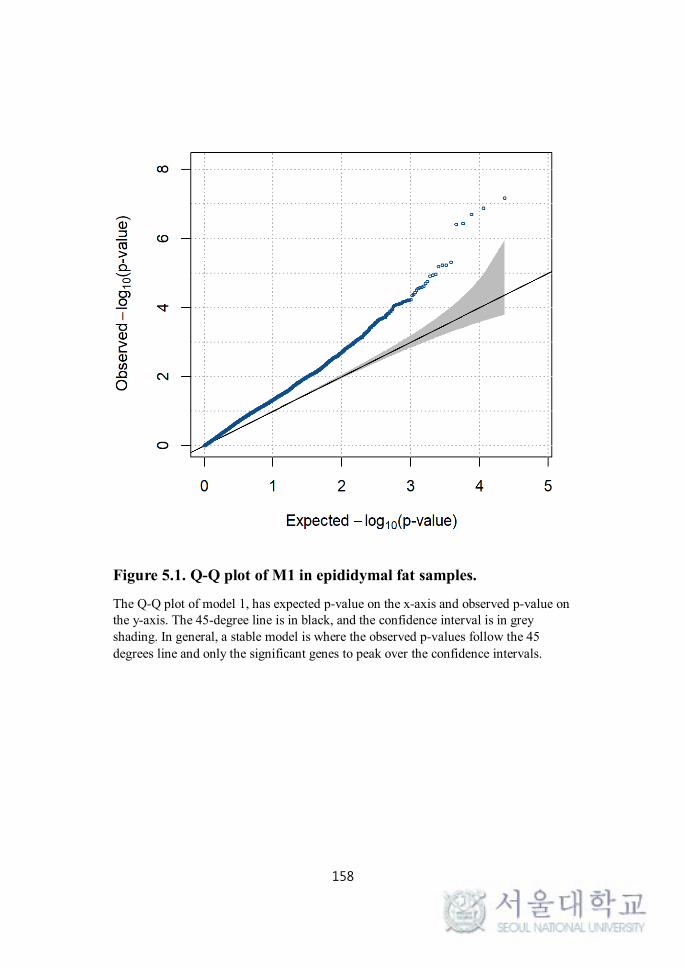
164

Figure 5.7. Expression pattern plots of a toggle gene (DEG-TAG) candidate.

The scatter plot (above) with the regression line shows the relationship between the gene expression and body weight. The box plot (below) shows the gene expression levels between groups. The plots are color-coded with HFD in orange, ALL in grey, and the ND in blue. The ND and ALL gene expression do not have a significant

statistical difference, yet the HFD group does.

165

Table 5.1 Functions of toggle genes.

Gene Tissue Function ReferenceAcoxl eWAT lipid metabolism GO

Mlec eWAT glycosylation(Schallus, Jaeckh et al. 2008)

Agt eWATinflammation, blood pressure, hypertension

(Vorkapic, Dugic et al. 2016)

Rbm17 eWAT Nucleotide binding N/ALamp1 eWAT Salla disease (Schleutker,

Haataja et al. 1991)

Car12 eWAT Non-related to diseases N/A

Arhgap11a Livercolon cancer, breast cancer cell line

RefSeq, GO

Gstm1 Liver liver cirrhosis, larynx cancer

(Jaskula-Sztul, Rienikainen et al. 1998)

Gstm2 Liver testis seminoma (Aceto, Di Ilio et al. 1989)

Limk1 Liverheart diseases and vein problems in the brain

(Yamada, Metoki et al. 2008)

Saa1 Liver tumor(Yang, Liu et al. 2016)

Saa2 Liver tumor(Yang, Liu et al. 2016)

RP23 361K13.1

Liver pseudo gene, not yet a functionN/A

Capn1 Liver chronic cervicitis, inflammation(Fukuta, Miyamoto et al. 2011)

Gsta1 Liver Inflammation, tumor(Chen, Tseng et al. 2010)

The least important genes have been grayed out.

166

5.4.2 Discussion

Although the data pricing has decreased and the quality went up,

scientists occasionally suffer from test results being not significant at

the multiple testing level. A conventional approach is to correct the

multiple testing problem with Bonferroni method, and if not enough

genes are significant, FDR is employed. When FDR does not work,

scientists work around by trying to decrease the number of tests as low

as possible. A hierarchical approach is a simple solution when we are

fusing two kinds of candidate lists (Cho, Kim et al. 2016). One can test

the A model and with the significant list from A, test the B model.

Since multiple testing correction is directly related to the number of

genes used for model B, such an approach can be more powerful than

merely getting the significant intersecting lists, at a given significance

level. Yet, we cannot overlook the fact that the raw p-value does not

change; which means, this is a matter of how to summarize and present

the given results. In this case, however, the candidates are only

significant at raw p-value level for TAGs and significant at FDR level

in the DEGs. The FDR significant DEGs are also significant at the

Bonferroni level, under the hierarchical condition, since the number of

tests is only 6 for the epididymal fat and 9 for the liver samples. We can

say that our toggle genes are significant DEGs at Bonferroni level and

167

TAGs at raw level. Bonferroni candidates are much more convincing

compared to those significant after FDR correction.

As the number of samples in RNA-seq studies increases with the data

quality and types, we will be able to access datasets that consist of

phenotypic traits and gene expression at multiple conditions. Our

hierarchical approach on linking TAGs and DEGs, as toggle genes, can

be used as a powerful summary technique to present the link between

traits and conditions with the differential expression of individuals.

168

Chapter 6. General Discussion

In the past decade, high-throughput techniques made dramatic

contributions to the elucidation of biological processes and mechanisms.

While conservatives might argue that there are many false positive

results among those publications, none are willing to cross-check the

validations provided by the authors of those publications. It is difficult

to check all the underlying assumptions and requirements of statistical

tools, and the required technical validations are temporary measures of

biological validations in actuality. Throughout the chapters, I illustrated

meta-analytical approaches that suggest study-specific biomarkers.

In chapter 2, I contributed to a GUI-program that compares multiple

test results to prune out the study-specific false positives and suggest

the most concordantly significant biomarkers such as DEGs. The study

has been applied to several platforms and data: (1) microarray dataset

with multiple test methods, (2) GWAS of NGS genome dataset with

multiple test methods, (3) RNA-seq dataset with multiple tools in R (4)

Family dataset of NGS genome with multiple test methods. As the

study was from my novice years as a bioinformatician, I neglected to

include factors like tissues or biological replicate data. The program

could be extended to cover those factors without changing the codes; it

will only require p-values from those tests, followed by an appropriate

169

interpretation. The program has been reviewed by several wet lab co-

workers, and have been introduced in a University level textbook

Epigenetic Gene Expression and Regulation by Blakey and Litt as a

useful tool in bioinformatics. I believe unprofessional researchers, in

terms of coding, can take advantage of our program in future research.

However, the user should have a clear understanding of the statistical

methods and what the globally significant biomarker means in their

study.

In chapter 3, I observed the potential errors in the current mRNA

expression quantification pipeline. Although some of the non-coding

RNAs such as miRNAs and lincRNAs have been elucidated in some

papers, none have connected those dots with RNA-seq analyses. The

problem rises where the lncRNA transcripts overlap with those of

mRNAs, more frequently on the opposite strand, and the annotations of

those transcripts therefore are overlapped. In addition, there are

numerous publications on how the lncRNA expression profiles are

tissue-specific, and I have confirmed the tissue-specific patterns in our

study. By comparing two pipelines—mRNA-only and mRNA-lncRNA

annotation—I analyzed four tissues, which were affected by the

inclusion of lncRNA differently. According to the results, the tissue of

interest is a factor in terms of overlapping reads, which are defined as

170

ambiguous reads in this study; the analysis results may or may not

contain substantial misquantification of mRNA expression levels. As

aforementioned, however, the downstream analyses are also affected by

such error, and the development of error pruning aligners and

quantifiers is imperative for accurate mRNA expression profiling and

differential expression analysis. I suggested using the concordantly

significant genes that are not affected by the change of annotation

pipelines for validations. While technical and biological validation

could have improved the study, a follow-up study of these mRNA-

lncRNA overlaps is in progress. Until an improvement in the

ambiguous read quantification is proposed, concurrent mRNA-seq

protocols are prone to the errors caused by the mRNA-lncRNA overlap.

The results from this study

In chapter 4, I focused on the study-defined inter-tissue crosstalk, or

interaction, between liver and epididymal fat (eWAT). We defined the

recovered genes (RecGs) and successfully validated the candidate

genes. The 20 RecGs are High-fat diet group-specific genes that imply

that the D-allulose intake helped to regulate the expression level back

to the normal level. Also, those genes have a significant positive

correlation with the Lactobacillus and Coprococcus, which are

inflammation-related microbiota. To present this information, I have

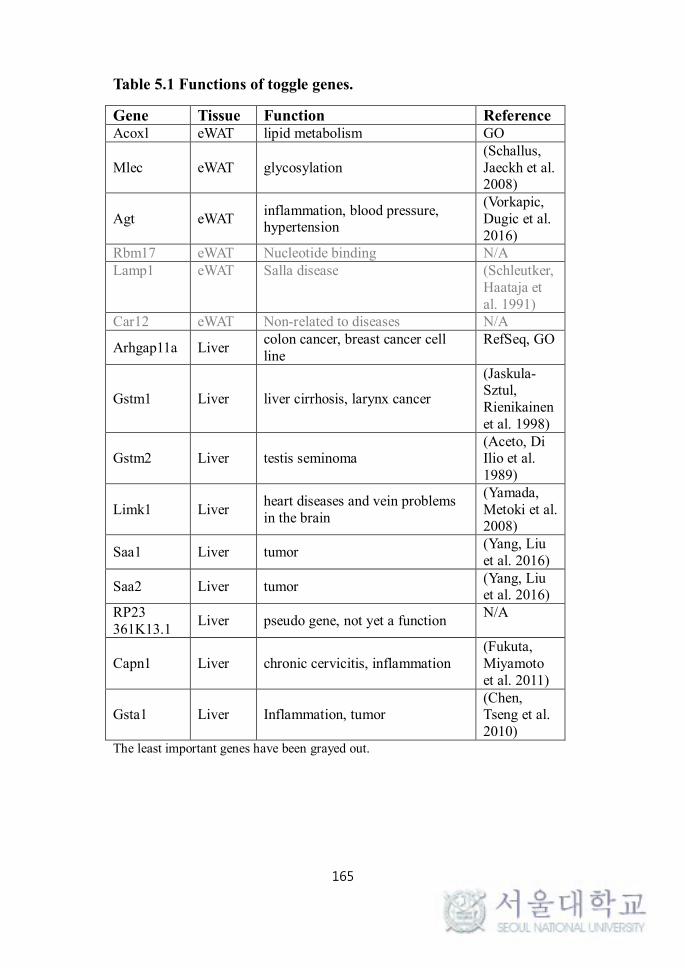
171

proposed a new plot that can handle p-value, fold change, and a factor

in the study. The factor we used in our study is the tissue, and inter-

tissue crosstalk could be clearly observed. I find it unfortunate that the

microbiome data in the analysis has been only used for quantification

and between-group testing by Wilcoxon, so the depth of the study could

have been improved if a more thorough analysis of the microbiome

data could have been incorporated.

In chapter 5, I have revisited an idea from two of my previous works

that handles differentially expressed genes (DEG)-phenotype-

associated genes (PAG) and DEG-trait-associated genes (TAGs). The

basic idea of PAG and TAG is the same except for the platform,

microarray and RNA-seq; the trait is used as the explanatory variable

instead of the gene expression levels. I have used the idea to perform

hierarchical approach to gain power in multiple testing adjustment.

Therefore, I could detect TAGs that were significant in raw p-value <

0.05, and DEG that are significant under Bonferroni adjusted p-value

level of 0.05. Although the TAGs are not significant under multiple

testing correction, it is well known that Bonferroni adjustments or FDR

adjustments can be conservative, and false negatives can arise. I used

the strict adjustment in the second-level DEG analysis (the first is TAG

analysis), using the TAG candidates only. In our study, only 6 in

172

epididymal fat and 9 in liver were carried on to the DEG analysis, and

all were found significant under Bonferroni levels. While the raw p-

values do not change, a non-hierarchical intersection method would

only define those genes to be significant at FDR adjusted levels, not

Bonferroni. The take-home message of this chapter is that the statistical

power can be gained by simple manipulation of a conventional pipeline,

and interpretation is always the key. Such hierarchical method can be

employed in any multi-class or multi-model integration studies.

All in all, in this thesis, I have presented numerous meta-analytical

techniques and pipelines that can be employed by many, to suggest

more formidable candidates in a more clear fashion to other researchers.

Simple adjustments to the original workflows can have considerable

effect visually and scientifically. I firmly believe some studies may

have been overlooked due to their lack of presentation and validity of

the candidates and hope my works can work as a stepping stone for the

publication of those works.

173

References

Aceto, A., C. Di Ilio, S. Angelucci, M. Felaco and G. Federici (1989). "Glutathione transferase isoenzymes from human testis." Biochem Pharmacol 38(21): 3653-3660.

Anders, S. and W. Huber (2010). "Differential expression analysis for sequence count data." Genome biol 11(10): R106.

Anders, S. and W. Huber (2012). "Differential expression of RNA-Seq data at the gene level–the DESeq package." Heidelberg, Germany: European Molecular Biology Laboratory (EMBL).

Anders, S., P. T. Pyl and W. Huber (2014). "HTSeq–A Python framework to work with high-throughput sequencing data." Bioinformatics: btu638.

Andersen, D. (2017). Interactions between host metabolism, immune regulation, and the gut microbiota in diet-associated obesity and metabolic dysfunction, Technical University of Denmark (DTU).

Andrews, S. (2014). FastQC A Quality Control tool for High Throughput Sequence Data.

Anhê, F. F., T. V. Varin, M. Le Barz, Y. Desjardins, E. Levy, D. Roy and A. Marette (2015). "Gut microbiota dysbiosis in obesity-linked metabolic diseases and prebiotic potential of polyphenol-rich extracts." Current obesity reports 4(4): 389-400.

Auer, P. L. and R. W. Doerge (2011). "A two-stage Poisson model for testing RNA-seq data." Statistical applications in genetics and molecular biology 10(1): 1-26.

Benjamini, Y. and Y. Hochberg (1995). "Controlling the false discovery rate: a practical and powerful approach to multiple testing." J R Stat Soc Ser B Methodol 57.

174

Bentley, D. R., S. Balasubramanian, H. P. Swerdlow, G. P. Smith, J. Milton, C. G. Brown, K. P. Hall, D. J. Evers, C. L. Barnes and H. R. Bignell (2008). "Accurate whole human genome sequencing using reversible terminator chemistry." nature 456(7218): 53-59.

Bolger, A. M., M. Lohse and B. Usadel (2014). "Trimmomatic: a flexible trimmer for Illumina sequence data." Bioinformatics 30.

Bolger, A. M., M. Lohse and B. Usadel (2014). "Trimmomatic: a flexible trimmer for Illumina sequence data." Bioinformatics: btu170.

Branton, D., D. W. Deamer, A. Marziali, H. Bayley, S. A. Benner, T. Butler, M. Di Ventra, S. Garaj, A. Hibbs, X. Huang, S. B. Jovanovich, P. S. Krstic, S. Lindsay, X. S. Ling, C. H. Mastrangelo, A. Meller, J. S. Oliver, Y. V. Pershin, J. M. Ramsey, R. Riehn, G. V. Soni, V. Tabard-Cossa, M. Wanunu, M. Wiggin and J. A. Schloss (2008). "The potential and challenges of nanopore sequencing." Nat Biotechnol 26(10): 1146-1153.

Bullard, J. H., E. Purdom, K. D. Hansen and S. Dudoit (2010). "Evaluation of statistical methods for normalization and differential expression in mRNA-Seq experiments." BMC bioinformatics 11(1): 94.

Cani, P. D., B. Rodrigo, C. Knauf, A. Waget, A. M. Neyrinck, N. M. Delzenne and R. Burcelin (2008). "Changes in gut microbiota control metabolic endotoxemia-induced inflammation in high-fat diet-induced obesity and diabetes in mice." Diabetes.

Chen, Y.-H., R.-B. Lu, H. Hung and P.-H. Kuo (2014). "Identifying Potential Regions of Copy Number Variation for Bipolar Disorder." Microarrays 3(1): 52-71.

Chen, Y. L., H. S. Tseng, W. H. Kuo, S. F. Yang, D. R. Chen and H. T. Tsai (2010). "Glutathione S-Transferase P1 (GSTP1) gene polymorphism increases age-related susceptibility to hepatocellular carcinoma." BMC Med Genet 11: 46.

175

Chitwood, J. L., G. Rincon, G. G. Kaiser, J. F. Medrano and P. J. Ross (2013). "RNA-seq analysis of single bovine blastocysts." BMC Genomics 14.

Cho, S. S., Y. Kim, J. Yoon, M. Seo, S.-k. Shin, E.-Y. Kwon, S.-E. Kim, Y.-J. Bae, S. Lee, M.-K. Sung, M.-S. Choi and T. Park (2016). "A Model-Based Joint Identification of Differentially Expressed Genes and Phenotype-Associated Genes." PLOS ONE 11(3): e0149086.

Choi, S., S. Lee, S. Cichon, M. M. Nothen, C. Lange, T. Park and S. Won (2014). "FARVAT: a family-based rare variant association test." Bioinformatics 30(22): 3197-3205.

Choi, S., S. Lee, M. M. Nöthen, C. Lange, T. Park and S. Won (2014). "FARVAT: a family-based rare variant association test." Bioinformatics: btu496.

Churchill, G. A. (2002). "Fundamentals of experimental design for cDNA microarrays." Nature genetics 32: 490-495.

Cui, X. and G. A. Churchill (2003). "Statistical tests for differential expression in cDNA microarray experiments." Genome Biol 4(4): 210.

Delzenne, N. M., A. M. Neyrinck, F. Bäckhed and P. D. Cani (2011). "Targeting gut microbiota in obesity: effects of prebiotics and probiotics." Nature Reviews Endocrinology 7(11): 639.

Derrien, T., R. Johnson, G. Bussotti, A. Tanzer, S. Djebali, H. Tilgner, G. Guernec, D. Martin, A. Merkel, D. G. Knowles, J. Lagarde, L. Veeravalli, X. Ruan, Y. Ruan, T. Lassmann, P. Carninci, J. B. Brown, L. Lipovich, J. M. Gonzalez, M. Thomas, C. A. Davis, R. Shiekhattar, T. R. Gingeras, T. J. Hubbard, C. Notredame, J. Harrow and R. Guigo (2012). "The GENCODE v7 catalog of human long noncoding RNAs: analysis of their gene structure, evolution, and expression." Genome Res 22(9): 1775-1789.

Di, Y., D. W. Schafer, J. S. Cumbie and J. H. Chang (2011). "The NBP

176

negative binomial model for assessing differential gene expression from RNA-Seq." Statistical Applications in Genetics and Molecular Biology 10(1): 1-28.

Dobin, A., C. A. Davis, F. Schlesinger, J. Drenkow, C. Zaleski, S. Jha, P. Batut, M. Chaisson and T. R. Gingeras (2013). "STAR: ultrafast universal RNA-seq aligner." Bioinformatics 29(1): 15-21.

English, A. C., S. Richards, Y. Han, M. Wang, V. Vee, J. Qu, X. Qin, D. M. Muzny, J. G. Reid, K. C. Worley and R. A. Gibbs (2012). "Mind the Gap: Upgrading Genomes with Pacific Biosciences RS Long-Read Sequencing Technology." PLOS ONE 7(11): e47768.

Etienne, W., M. H. Meyer, J. Peppers and R. A. Meyer, Jr. (2004). "Comparison of mRNA gene expression by RT-PCR and DNA microarray." Biotechniques 36(4): 618-620, 622, 624-616.

Fang, Z. and X. Cui (2011). "Design and validation issues in RNA-seq experiments." Briefings in bioinformatics: bbr004.

Fisher, R. A. (2006). Statistical methods for research workers, Genesis Publishing Pvt Ltd.

Flegal, K. M., D. Kruszon-Moran, M. D. Carroll, C. D. Fryar and C. L. Ogden (2016). "Trends in Obesity Among Adults in the United States, 2005 to 2014." Jama 315(21): 2284-2291.

Forster, T., D. Roy and P. Ghazal (2003). "Experiments using microarray technology: limitations and standard operating procedures." Journal of endocrinology 178(2): 195-204.

Fukuta, S., K. Miyamoto, K. Suzuki, H. Maehara, T. Inoue, A. Hara, K. Kikuike, A. Taguchi and K. Shimizu (2011). "Abundance of calpain and aggrecan-cleavage products of calpain in degenerated human intervertebral discs." Osteoarthritis Cartilage 19(10): 1254-1262.

177

Gómez, E., J. N. Caamaño, F. J. Corrales, C. Díez, E. Correia-Álvarez and D. Martín (2013). "Embryonic sex induces differential expression of proteins in bovine uterine fluid." J Proteome Res 12.

Garber, M., M. G. Grabherr, M. Guttman and C. Trapnell (2011). "Computational methods for transcriptome annotation and quantification using RNA-seq." Nature methods 8(6): 469-477.

Gibbs, R. A., J. W. Belmont, P. Hardenbol, T. D. Willis, F. Yu, H. Yang, L.-Y. Ch'ang, W. Huang, B. Liu and Y. Shen (2003). "The international HapMap project." Nature 426(6968): 789-796.

Gill, J. L., S. C. Bishop, C. McCorquodale, J. L. Williams and P. Wiener (2009). "Association of selected SNP with carcass and taste panel assessed meat quality traits in a commercial population of Aberdeen Angus-sired beef cattle." Genet Sel Evol 41.

Grabherr, M. G., B. J. Haas, M. Yassour, J. Z. Levin, D. A. Thompson, I. Amit, X. Adiconis, L. Fan, R. Raychowdhury and Q. Zeng (2011). "Full-length transcriptome assembly from RNA-Seq data without a reference genome." Nature biotechnology 29(7): 644-652.

Grant, G. R., M. H. Farkas, A. D. Pizarro, N. F. Lahens, J. Schug, B. P. Brunk, C. J. Stoeckert, J. B. Hogenesch and E. A. Pierce (2011). "Comparative analysis of RNA-Seq alignment algorithms and the RNA-Seq unified mapper (RUM)." Bioinformatics 27(18): 2518-2528.

Grundy, S. M. (2004). "Obesity, metabolic syndrome, and cardiovascular disease." The Journal of Clinical Endocrinology & Metabolism 89(6): 2595-2600.

Han, Y., H. J. Han, A. H. Kim, J. Y. Choi, S. J. Cho, Y. B. Park, U. J. Jung and M. S. Choi (2016). "d‐Allulose supplementation normalized the body weight and fat‐pad mass in diet‐induced obese mice via the regulation of lipid metabolism under isocaloric fed condition." Molecular nutrition & food research 60(7): 1695-1706.

178

Handa, R. J., L. H. Burgess, J. E. Kerr and J. A. O’Keefe (1994). "Gonadal steroid hormone receptors and sex differences in the hypothalamo-pituitary-adrenal axis." Horm Behav 28.

Hansen, K. D., R. A. Irizarry and W. Zhijin (2012). "Removing technical variability in RNA-seq data using conditional quantile normalization." Biostatistics 13(2): 204-216.

Hirschhorn, J. N. and M. J. Daly (2005). "Genome-wide association studies for common diseases and complex traits." Nat Rev Genet 6(2): 95-108.

Hossain, M. A., S. Kitagaki, D. Nakano, A. Nishiyama, Y. Funamoto, T. Matsunaga, I. Tsukamoto, F. Yamaguchi, K. Kamitori and Y. Dong (2011). "Rare sugar D-psicose improves insulin sensitivity and glucose tolerance in type 2 diabetes Otsuka Long-Evans Tokushima Fatty (OLETF) rats." Biochemical and biophysical research communications405(1): 7-12.

Howe, E., K. Holton, S. Nair, D. Schlauch, R. Sinha and J. Quackenbush (2010). MeV: multiExperiment viewer. Biomedical Informatics for Cancer Research, Springer: 267-277.

Huang, D. W., B. T. Sherman and R. A. Lempicki (2009). "Systematic and integrative analysis of large gene lists using DAVID bioinformatics resources." Nature Protocols 4(1): 44-57.

Humphreys, D. T. and C. M. Suter (2013). "miRspring: a compact standalone research tool for analyzing miRNA-seq data." Nucleic acids research 41(15): e147-e147.

Hursting, S. D. and M. J. Hursting (2012). "Growth signals, inflammation, and vascular perturbations: mechanistic links between obesity, metabolic syndrome, and cancer." Arteriosclerosis, thrombosis, and vascular biology 32(8): 1766-1770.

Immonen, E., A. Sayadi, H. Bayram and G. Arnqvist (2017). "Mating

179

Changes Sexually Dimorphic Gene Expression in the Seed Beetle Callosobruchus maculatus." Genome Biology and Evolution 9(3): 677-699.

Iwakiri, J., G. Terai and M. Hamada (2017). "Computational prediction of lncRNA-mRNA interactions by integrating tissue specificity in human transcriptome." Biology Direct 12(1): 15.

Iyengar, N. M., A. Gucalp, A. J. Dannenberg and C. A. Hudis (2016). "Obesity and cancer mechanisms: tumor microenvironment and inflammation." Journal of clinical oncology 34(35): 4270.

Jaskula-Sztul, R., M. Rienikainen, K. Husgafvel-Pursiainen, Z. Szmeja, W. Szyfter, K. Syfter and A. Hirvonen (1998). "Glutathione S transferase M1 andT1 genotypes and susceptibility to smoking related larynx cancer." Biomarkers 3(2): 149-155.

Jiang, Y. A. and H. P. Zhang (2011). "Propensity Score-Based Nonparametric Test Revealing Genetic Variants Underlying Bipolar Disorder." Genetic Epidemiology 35(2): 125-132.

Jung, U. J. and M.-S. Choi (2014). "Obesity and its metabolic complications: the role of adipokines and the relationship between obesity, inflammation, insulin resistance, dyslipidemia and nonalcoholic fatty liver disease." International journal of molecular sciences 15(4): 6184-6223.

Kim, D., B. Langmead and S. L. Salzberg (2015). "HISAT: a fast spliced aligner with low memory requirements." Nature Methods 12: 357.

Kim, N.-H., H.-J. Kim, D.-I. Kang, K.-W. Jeong, J.-K. Lee, Y. Kim and D.-K. Oh (2008). "Conversion shift of D-fructose to D-psicose for enzyme-catalyzed epimerization by addition of borate." Applied and environmental microbiology 74(10): 3008-3013.

Kozarewa, I., Z. Ning, M. A. Quail, M. J. Sanders, M. Berriman and D.

180

J. Turner (2009). "Amplification-free Illumina sequencing-library preparation facilitates improved mapping and assembly of (G+C)-biased genomes." Nat Methods 6(4): 291-295.

Kuczynski, J., J. Stombaugh, W. A. Walters, A. González, J. G. Caporaso and R. Knight (2011). "Using QIIME to analyze 16S rRNA gene sequences from microbial communities." Current protocols in bioinformatics Chapter 10: Unit10.17-10.17.

Kwon, M.-S., M. Park and T. Park (2014). "IGENT: efficient entropy based algorithm for genome-wide gene-gene interaction analysis." BMC Medical Genomics 7(Suppl 1): S6.

LaBreche, H. G., J. R. Nevins and E. Huang (2011). "Integrating Factor Analysis and a Transgenic Mouse Model to Reveal a Peripheral Blood Predictor of Breast Tumors." Bmc Medical Genomics 4.

Langmead, B. and S. L. Salzberg (2012). "Fast gapped-read alignment with Bowtie 2." Nature methods 9(4): 357-359.

Lee, S., M. J. Emond, M. J. Bamshad, K. C. Barnes, M. J. Rieder, D. A. Nickerson, D. C. Christiani, M. M. Wurfel and X. Lin (2012). "Optimal unified approach for rare-variant association testing with application to small-sample case-control whole-exome sequencing studies." The American Journal of Human Genetics 91(2): 224-237.

Li, A., J. Zhang, Z. Zhou, L. Wang, Y. Liu and Y. Liu (2015). "ALDB: A Domestic-Animal Long Noncoding RNA Database." PLOS ONE10(4): e0124003.

Li, H. and R. Durbin (2009). "Fast and accurate short read alignment with Burrows–Wheeler transform." Bioinformatics 25(14): 1754-1760.

Liao, Y., G. K. Smyth and W. Shi (2014). "featureCounts: an efficient general purpose program for assigning sequence reads to genomic features." Bioinformatics 30(7): 923-930.

181

Lindgreen, S. (2012). "AdapterRemoval: easy cleaning of next-generation sequencing reads." BMC research notes 5(1): 337.

Love, M. I., W. Huber and S. Anders (2014). "Moderated estimation of fold change and dispersion for RNA-seq data with DESeq2." Genome Biol 15(12): 550.

Lu, T., G. Lu, D. Fan, C. Zhu, W. Li, Q. Zhao, Q. Feng, Y. Zhao, Y. Guo and W. Li (2010). "Function annotation of the rice transcriptome at single-nucleotide resolution by RNA-seq." Genome research 20(9): 1238-1249.

Marioni, J. C., C. E. Mason, S. M. Mane, M. Stephens and Y. Gilad (2008). "RNA-seq: an assessment of technical reproducibility and comparison with gene expression arrays." Genome Res 18(9): 1509-1517.

Maxam, A. M. and W. Gilbert (1977). "A new method for sequencing DNA." Proc Natl Acad Sci U S A 74(2): 560-564.

McCarthy, D. J. and G. K. Smyth (2009). "Testing significance relative to a fold-change threshold is a TREAT." Bioinformatics (Oxford, England) 25(6): 765-771.

Meisel, J. S., G. Sfyroera, C. Bartow-McKenney, C. Gimblet, J. Bugayev, J. Horwinski, B. Kim, J. R. Brestoff, A. S. Tyldsley, Q. Zheng, B. P. Hodkinson, D. Artis and E. A. Grice (2018). "Commensal microbiota modulate gene expression in the skin." Microbiome 6(1): 20-20.

Metzker, M. L. (2010). "Sequencing technologies - the next generation." Nat Rev Genet 11(1): 31-46.

Mokdad, A. H., E. S. Ford, B. A. Bowman, W. H. Dietz, F. Vinicor, V. S. Bales and J. S. Marks (2003). "Prevalence of obesity, diabetes, and obesity-related health risk factors, 2001." Jama 289(1): 76-79.

182

Monteiro, R. and I. Azevedo (2010). "Chronic inflammation in obesity and the metabolic syndrome." Mediators of inflammation 2010.

Moreno-Indias, I., L. Sánchez-Alcoholado, P. Pérez-Martínez, C. Andrés-Lacueva, F. Cardona, F. Tinahones and M. I. Queipo-Ortuño (2016). "Red wine polyphenols modulate fecal microbiota and reduce markers of the metabolic syndrome in obese patients." Food & function7(4): 1775-1787.

Morey, J. S., J. C. Ryan and F. M. Van Dolah (2006). "Microarray validation: factors influencing correlation between oligonucleotide microarrays and real-time PCR." Biological procedures online 8: 175-193.

Morgan, X. C., B. Kabakchiev, L. Waldron, A. D. Tyler, T. L. Tickle, R. Milgrom, J. M. Stempak, D. Gevers, R. J. Xavier, M. S. Silverberg and C. Huttenhower (2015). "Associations between host gene expression, the mucosal microbiome, and clinical outcome in the pelvic pouch of patients with inflammatory bowel disease." Genome Biol 16: 67.

Morozova, O., M. Hirst and M. A. Marra (2009). "Applications of new sequencing technologies for transcriptome analysis." Annu Rev Genomics Hum Genet 10: 135-151.

Mortazavi, A., B. A. Williams, K. McCue, L. Schaeffer and B. Wold (2008). "Mapping and quantifying mammalian transcriptomes by RNA-Seq." Nature methods 5(7): 621-628.

Mortazavi, A., B. A. Williams, K. McCue, L. Schaeffer and B. Wold (2008). "Mapping and quantifying mammalian transcriptomes by RNA-Seq." Nat Methods 5(7): 621-628.

Muret, K., C. Klopp, V. Wucher, D. Esquerré, F. Legeai, F. Lecerf, C. Désert, M. Boutin, F. Jehl, H. Acloque, E. Giuffra, S. Djebali, S. Foissac, T. Derrien and S. Lagarrigue (2017). "Long noncoding RNA repertoire in chicken liver and adipose tissue." Genet Sel Evol 49.

183

Mwai, O., O. Hanotte, Y.-J. Kwon and S. Cho (2015). "African indigenous cattle: unique genetic resources in a rapidly changing world." Asian-Australas J Anim Sci 28.

Nagato, T., H. Kobayashi, K. Kishibe, M. Takahara, T. Ogino, H. Ishii, K. Oikawa, N. Aoki, K. Sato, S. Kimura, N. Shimizu, M. Tateno and Y. Harabuchi (2005). "Expression of interleukin-9 in nasal natural killer/T-cell lymphoma cell lines and patients." Clinical Cancer Research 11(23): 8250-8257.

Nagato, T., H. Kobayashi, K. Kishibe, M. Takahara, T. Ogino, H. Ishii, K. Oikawa, N. Aoki, K. Sato, S. Kimura, N. Shimizu, M. Tateno and Y. Harabuchi (2005). "Expression of interleukin-9 in nasal natural killer/T-cell lymphoma cell lines and patients." Clin Cancer Res 11(23): 8250-8257.

Neale, B. M., M. A. Rivas, B. F. Voight, D. Altshuler, B. Devlin, M. Orho-Melander, S. Kathiresan, S. M. Purcell, K. Roeder and M. J. Daly (2011). "Testing for an unusual distribution of rare variants." PLoS genetics 7(3): e1001322.

Nelder, J. A. a. B., R.J. (2006). Generalized Linear Models. Encyclopedia of Statistical Sciences. C. B. R. S. Kotz, N. Balakrishnan, B. Vidakovic and N. L. Johnson.

Nishida, Y., M. Yoshioka and J. St-Amand (2005). "Sexually dimorphic gene expression in the hypothalamus, pituitary gland, and cortex." Genomics 85.

Nookaew, I., M. Papini, N. Pornputtpong, G. Scalcinati, L. Fagerberg, M. Uhlén and J. Nielsen (2012). "A comprehensive comparison of RNA-Seq-based transcriptome analysis from reads to differential gene expression and cross-comparison with microarrays: a case study in Saccharomyces cerevisiae." Nucleic acids research: gks804.

Oh, S., J. Lee, M. S. Kwon, B. Weir, K. Ha and T. Park (2012). "A novel method to identify high order gene-gene interactions in genome-

184

wide association studies: Gene-based MDR." Bmc Bioinformatics 13.

Palo, O. M. (2010). "Genetic background of bipolar disorder and related cognitive impairments."

Pan, W. (2002). "A comparative review of statistical methods for discovering differentially expressed genes in replicated microarray experiments." Bioinformatics 18(4): 546-554.

PATANI, N., W. JIANG and K. MOKBEL (2008). "Prognostic utility of glycosyltransferase expression in breast cancer." Cancer Genomics-Proteomics 5(6): 333-340.

Polak, J., E. Klimcakova, C. Moro, N. Viguerie, M. Berlan, J. Hejnova, B. Richterova, I. Kraus, D. Langin and V. Stich (2006). "Effect of aerobic training on plasma levels and subcutaneous abdominal adipose tissue gene expression of adiponectin, leptin, interleukin 6, and tumor necrosis factor α in obese women." Metabolism 55(10): 1375-1381.

Purcell, S., B. Neale, K. Todd-Brown, L. Thomas, M. A. R. Ferreira, D. Bender, J. Maller, P. Sklar, P. I. W. de Bakker, M. J. Daly and P. C. Sham (2007). "PLINK: A tool set for whole-genome association and population-based linkage analyses." American Journal of Human Genetics 81(3): 559-575.

Rajeevan, M. S., S. D. Vernon, N. Taysavang and E. R. Unger (2001). "Validation of array-based gene expression profiles by real-time (kinetic) RT-PCR." J Mol Diagn 3(1): 26-31.

Rapaport, F., R. Khanin, Y. Liang, M. Pirun, A. Krek, P. Zumbo, C. E. Mason, N. D. Socci and D. Betel (2013). "Comprehensive evaluation of differential gene expression analysis methods for RNA-seq data." Genome Biol 14(9): R95.

Rhodes, M. E. and R. T. Rubin (1999). "Functional sex differences (sexual diergism’) of central nervous system cholinergic systems, vasopressin, and hypothalamic–pituitary–adrenal axis activity in

185

mammals: a selective review." Brain Res Rev 30.

Richards, A., A. L. Muehlbauer, A. Alazizi, M. B. Burns, A. Findley, F. Messina, T. J. Gould, C. Cascardo, R. Pique-Regi, R. Blekhman and F. Luca (2018). "Gut microbiota has a widespread and modifiable effect on host gene regulation." bioRxiv.

Risso, D., K. Schwartz, G. Sherlock and S. Dudoit (2011). "GC-content normalization for RNA-Seq data." BMC bioinformatics 12(1): 480.

Roberts, A., H. Pimentel, C. Trapnell and L. Pachter (2011). "Identification of novel transcripts in annotated genomes using RNA-Seq." Bioinformatics 27(17): 2325-2329.

Robinson, M. D., D. J. McCarthy and G. K. Smyth (2010). "edgeR: a Bioconductor package for differential expression analysis of digitalgene expression data." Bioinformatics 26.

Robinson, M. D., D. J. McCarthy and G. K. Smyth (2010). "edgeR: a Bioconductor package for differential expression analysis of digital gene expression data." Bioinformatics 26(1): 139-140.

Robinson, M. D. and A. Oshlack (2010). "A scaling normalization method for differential expression analysis of RNA-seq data." Genome biology 11(3): R25-R25.

Robinson, M. D. and A. Oshlack (2010). "A scaling normalization method for differential expression analysis of RNA-seq data." Genome Biol 11(3): R25.

Robinson, M. D. and G. K. Smyth (2008). "Small-sample estimation of negative binomial dispersion, with applications to SAGE data." Biostatistics 9(2): 321-332.

Rothberg, J. M., W. Hinz, T. M. Rearick, J. Schultz, W. Mileski, M. Davey, J. H. Leamon, K. Johnson, M. J. Milgrew, M. Edwards, J. Hoon,

186

J. F. Simons, D. Marran, J. W. Myers, J. F. Davidson, A. Branting, J. R. Nobile, B. P. Puc, D. Light, T. A. Clark, M. Huber, J. T. Branciforte, I. B. Stoner, S. E. Cawley, M. Lyons, Y. Fu, N. Homer, M. Sedova, X. Miao, B. Reed, J. Sabina, E. Feierstein, M. Schorn, M. Alanjary, E. Dimalanta, D. Dressman, R. Kasinskas, T. Sokolsky, J. A. Fidanza, E. Namsaraev, K. J. McKernan, A. Williams, G. T. Roth and J. Bustillo (2011). "An integrated semiconductor device enabling non-optical genome sequencing." Nature 475: 348.

Rothberg, J. M. and J. H. Leamon (2008). "The development and impact of 454 sequencing." Nat Biotechnol 26(10): 1117-1124.

Sanchez-Cardenas, C., P. Fontanaud, Z. He, C. Lafont, A.-C. Meunier and M. Schaeffer (2010). "Pituitary growth hormone network responses are sexually dimorphic and regulated by gonadal steroids in adulthood." Proc Natl Acad Sci 107.

Sanger, F., S. Nicklen and A. R. Coulson (1977). "DNA sequencing with chain-terminating inhibitors." Proc Natl Acad Sci U S A 74(12): 5463-5467.

Schallus, T., C. Jaeckh, K. Feher, A. S. Palma, Y. Liu, J. C. Simpson, M. Mackeen, G. Stier, T. J. Gibson, T. Feizi, T. Pieler and C. Muhle-Goll (2008). "Malectin: a novel carbohydrate-binding protein of the endoplasmic reticulum and a candidate player in the early steps of protein N-glycosylation." Mol Biol Cell 19(8): 3404-3414.

Schleutker, J., L. Haataja, M. Renlund, L. Puhakka, J. Viitala, L. Peltonen and P. Aula (1991). "Confirmation of the chromosomal localization of human lamp genes and their exclusion as candidate genes for Salla disease." Hum Genet 88(1): 95-97.

Schwiertz, A., D. Taras, K. Schafer, S. Beijer, N. A. Bos, C. Donus and P. D. Hardt (2010). "Microbiota and SCFA in lean and overweight healthy subjects." Obesity (Silver Spring) 18(1): 190-195.

Seo, M., K. Caetano-Anolles, S. Rodriguez-Zas, S. Ka, J. Y. Jeong, S.

187

Park, M. J. Kim, W.-G. Nho, S. Cho, H. Kim and H.-J. Lee (2016). "Comprehensive identification of sexually dimorphic genes in diverse cattle tissues using RNA-seq." BMC Genomics 17(1): 81.

Seo, M., K. Kim, J. Yoon, J. Y. Jeong, H.-J. Lee, S. Cho and H. Kim (2016). "RNA-seq analysis for detecting quantitative trait-associated genes." Scientific Reports 6: 24375.

Shapiro, S. S. and M. B. Wilk (1965). "An Analysis of Variance Test for Normality (Complete Samples)." Biometrika 52(3/4): 591-611.

Sherry, S. T., M.-H. Ward, M. Kholodov, J. Baker, L. Phan, E. M. Smigielski and K. Sirotkin (2001). "dbSNP: the NCBI database of genetic variation." Nucleic acids research 29(1): 308-311.

Shintani, T., T. Yamada, N. Hayashi, T. Iida, Y. Nagata, N. Ozaki and Y. Toyoda (2017). "Rare sugar syrup containing D-allulose but not high-fructose corn syrup maintains glucose tolerance and insulin sensitivity partly via hepatic glucokinase translocation in Wistar rats." Journal of agricultural and food chemistry 65(13): 2888-2894.

Smith, L. M., J. Z. Sanders, R. J. Kaiser, P. Hughes, C. Dodd, C. R. Connell, C. Heiner, S. B. Kent and L. E. Hood (1986). "Fluorescence detection in automated DNA sequence analysis." Nature 321(6071): 674-679.

Soneson, C. and M. Delorenzi (2013). "A comparison of methods for differential expression analysis of RNA-seq data." BMC bioinformatics14(1): 91.

Splan, R. K., L. V. Cundiff and L. D. Vleck (1998). "Genetic parameters for sex-specific traits in beef cattle." J Anim Sci 76.

Sreekumar, J. and K. Jose (2008). "Statistical tests for identification of differentially expressed genes in cDNA microarray experiments." Indian Journal of Biotechnology 7(4): 423-436.

188

Tilgner, H., D. G. Knowles, R. Johnson, C. A. Davis, S. Chakrabortty, S. Djebali, J. Curado, M. Snyder, T. R. Gingeras and R. Guigó (2012). "Deep sequencing of subcellular RNA fractions shows splicing to be predominantly co-transcriptional in the human genome but inefficient for lncRNAs." Genome research 22(9): 1616-1625.

Trapnell, C., L. Pachter and S. L. Salzberg (2009). "TopHat: discovering splice junctions with RNA-Seq." Bioinformatics 25(9): 1105-1111.

Trapnell, C., A. Roberts, L. Goff, G. Pertea, D. Kim, D. R. Kelley, H. Pimentel, S. L. Salzberg, J. L. Rinn and L. Pachter (2012). "Differential gene and transcript expression analysis of RNA-seq experiments with TopHat and Cufflinks." Nature protocols 7(3): 562-578.

Travers, K. J., C. S. Chin, D. R. Rank, J. S. Eid and S. W. Turner (2010). "A flexible and efficient template format for circular consensus sequencing and SNP detection." Nucleic Acids Res 38(15): e159.

Troyanskaya, O. G., M. E. Garber, P. O. Brown, D. Botstein and R. B. Altman (2002). "Nonparametric methods for identifying differentially expressed genes in microarray data." Bioinformatics 18(11): 1454-1461.

Tusher, V. G., R. Tibshirani and G. Chu (2001). "Significance analysis of microarrays applied to the ionizing radiation response." Proceedings of the National Academy of Sciences of the United States of America98(9): 5116-5121.

Vêncio, R. Z., H. Brentani, D. F. Patrão and C. A. Pereira (2004). "Bayesian model accounting for within-class biological variability in Serial Analysis of Gene Expression (SAGE)." BMC bioinformatics5(1): 119.

Vitale, L., F. Frabetti, S. A. Huntsman, S. Canaider, R. Casadei, L. Lenzi, F. Facchin, P. Carinci, M. Zannotti, D. Coppola and P. Strippoli (2007). "Sequence, "subtle" alternative splicing and expression of the CYYR1 (cysteine/tyrosine-rich 1) mRNA in human neuroendocrine

189

tumors." BMC Cancer 7: 66.

Vitale, L., F. Frabetti, S. A. Huntsman, S. Canaider, R. Casadei, L. Lenzi, F. Facchin, P. Carinci, M. Zannotti, D. Coppola and P. Strippoli (2007). "Sequence, "subtle" alternative splicing and expression of theCYYR1 (cysteine/tyrosine-rich 1) mRNA in human neuroendocrine tumors." Bmc Cancer 7.

Vorkapic, E., E. Dugic, S. Vikingsson, J. Roy, M. I. Mayranpaa, P. Eriksson and D. Wagsater (2016). "Imatinib treatment attenuates growth and inflammation of angiotensin II induced abdominal aortic aneurysm." Atherosclerosis 249: 101-109.

Voskoboynik, A., N. F. Neff, D. Sahoo, A. M. Newman, D. Pushkarev, W. Koh, B. Passarelli, H. C. Fan, G. L. Mantalas, K. J. Palmeri, K. J. Ishizuka, C. Gissi, F. Griggio, R. Ben-Shlomo, D. M. Corey, L. Penland, R. A. White, III, I. L. Weissman and S. R. Quake (2013). "The genome sequence of the colonial chordate, Botryllus schlosseri." eLife 2: e00569.

Wang, Z., M. Gerstein and M. Snyder (2009). "RNA-Seq: a revolutionary tool for transcriptomics." Nature Reviews Genetics 10(1): 57-63.

Wei Huang, B. T. S. and R. A. Lempicki (2008). "Systematic and integrative analysis of large gene lists using DAVID bioinformatics resources." Nat Protoc 4.

Wu, M. C., S. Lee, T. Cai, Y. Li, M. Boehnke and X. Lin (2011). "Rare-variant association testing for sequencing data with the sequence kernel association test." The American Journal of Human Genetics 89(1): 82-93.

Wurmbach, E., T. Yuen and S. C. Sealfon (2003). "Focused microarray analysis." Methods 31(4): 306-316.

Yamada, Y., N. Metoki, H. Yoshida, K. Satoh, K. Kato, T. Hibino, K.

190

Yokoi, S. Watanabe, S. Ichihara, Y. Aoyagi, A. Yasunaga, H. Park, M. Tanaka and Y. Nozawa (2008). "Genetic factors for ischemic and hemorrhagic stroke in Japanese individuals." Stroke 39(8): 2211-2218.

Yang, M., F. Liu, K. Higuchi, J. Sawashita, X. Fu, L. Zhang, L. Zhang, L. Fu, Z. Tong and K. Higuchi (2016). "Serum amyloid A expression in the breast cancer tissue is associated with poor prognosis." Oncotarget7(24): 35843-35852.

Yang, X., E. E. Schadt, S. Wang, H. Wang, A. P. Arnold and L. Ingram-Drake (2006). "Tissue-specific expression and regulation of sexually dimorphic genes in mice." Genome Res 16.

You, T., R. Yang, M. F. Lyles, D. Gong and B. J. Nicklas (2005). "Abdominal adipose tissue cytokine gene expression: relationship to obesity and metabolic risk factors." American Journal of Physiology-Endocrinology and Metabolism 288(4): E741-E747.

Zhang, L., N. Li, R. Caicedo and J. Neu (2005). "Alive and dead Lactobacillus rhamnosus GG decrease tumor necrosis factor-α–induced interleukin-8 production in caco-2 cells." The Journal of nutrition135(7): 1752-1756.

Zhang, Y., L. Yang and L.-L. Chen (2014). "Life without A tail: New formats of long noncoding RNAs." The International Journal of Biochemistry & Cell Biology 54: 338-349.

Zhu, Y., M. Li, A. M. Sousa and N. Šestan (2014). "XSAnno: a framework for building ortholog models in cross-species transcriptome comparisons." BMC genomics 15(1): 343.

191

요약 (국문 초록)

메타분석 전략을 활용한 전사체상 바이오마커의

선별

윤준

협동과정 생물정보학 전공


차세대 염기서열 분석은 생물정보학을 포함한 생명과학 분야

에 기술적으로나 지식적으로 비약적인 발전을 가져왔다. 또한,

차세대 염기서열 분석은 그 신속성과 저렴한 비용으로 인해

수많은 생물학적 데이터의 생산과 이에 관한 연구에 활용되어

왔다. 이는 필연적으로 대용량 자료를 분석할 수 있는 복잡한

통계적 분석 기법의 발전으로 이어졌으며, 생물정보학 이라는

신생 분야의 발전을 촉진하는 원동력이 되었다. 그러나 복잡한

대용량 자료구조 및 통계적 분석 기법은 연구설계나 내용에

대한 직관적인 이해를 방해할 뿐만 아니라, 특히 생물정보학을

도구로서 활용하는 비전공자의 연구에 커다란 걸림돌이 된다.

따라서 메타분석을 사용한 적합한 통계 모형 구축과 바이오마

커 선별 같은 생물정보학적 분석파이프라인은 연구자의 연구

192

내용과 자료를 잘 대변해 줄 수 있어야 한다. 현재, 분석 방법

론과 프로그램은 많이 제시되어 있는 상태이지만, 이러한 기술

들을 연구자가 실제 연구에 어떻게 효과적으로 적용할 것인가

는 자료 특이적이며, 그 분석결과의 해석은 여전히 연구자의

재량에 달려있다.

이 학위논문은 다양한 실험설계 상황에서 각각의 설계에 부합

하는 의미 있는 후보 유전자를 발굴해 내기 위한 메타분석기

법을 중점을 두고 있다. 2장에서는 생물정보학 분석에서 p값

에 대한 메타 분석을 다루고 있다. 특히, 다양한 통계 모형과

검증에서 나온 결과를 비교 및 통합할 수 있는 시각화 방법과

여러 독립된 통계검증 결과에서 동시에 유의한 후보 유전자를

발굴하는 예제를 다루고 있다. 또한 이 장에서 제시된 기법을

사용한 GUI (Graphic User Interface) 기반 프로그램을

microarray, GWAS, RNA-seq, 가족 기반 데이터 등 다양한

형태의 데이터에 적용함으로써, 제시된 프로그램이 p값을 포

함한 다양한 통계치에 기반한 연구에 활용될 수 있음을 보였

다.

3장에서는 mRNA-seq 데이터 분석에서 long non-coding

RNA (lncRNA) 를 고려하지 않음으로써 생기는 분석결과의

193

문제점과 이에 타격을 입지 않는 바이오마커 선별을 다루고

있다. 일반적으로 mRNA-seq 프로토콜에서 mRNA를 선택적

으로 분리해 내는 방법은 poly-A tail을 이용한다. 그러나

lncRNA를 포함한 일부 non-coding RNA 들도 mRNA 와 마

찬가지로 전사과정에서 poly-A tail을 가진다. 이러한 경우에

RNA-seq 데이터 내에서 lncRNA 와 mRNA 는 명확히 구분

되지 않는다. 이 장에서는 RNA-seq 데이터 분석과정에서

lncRNA annotation 의 고려 유무가 최종 결과인 차등 발현

유전자 결과에 상당한 영향을 미친다는 것을 보여줌으로써,

lncRNA를 고려하지 않은 기존의 분석방법이 후보 유전자 발

굴에 변수가 될 수 있음을 밝혔다. 더불어, lncRNA

annotation이 후보 유전자 결과에 미치는 영향은 조직 별로

다른 양상을 나타낸다는 것을 두 개의 독립적인 차등발현 유

전자 분석방법을 통해 보여주었다. 결론적으로 lncRNA

annotation 정보의 영향을 받지 않는 유전자들이 mRNA-seq

실험설계목적에 가장 부합되는 후보 유전자 임을 제시하였다.

4장에서는 항 염증과 비만에 효과를 보이는 감미료를 먹인 쥐

에 대한 RNA-seq및 Metagenome 분석을 통해 실험 목적에

부합하는 후보유전자발굴 과정을 다루었다. 정상식이집단

194

(ND), 고지방식이집단 (HFD), D-allulose와 고지방식이집단

(ALL) 에 대해 각각 2개의 조직을 사용하였으며, 고지방식이

에 대한 D-allulose의 효과와 밀접하게 관련된 후보유전자를

발굴하기 위하여 “Recovery gene” (RecG) 을 정의하였다.

RecG 은 개념적으로 고지방식이의 유전자 발현 상태에서 D-

allulose를 섭취했을 때 정상상태로 돌아가는 유전자를 말하여,

실제 분석에서는 두 조직 모두에서 HFD 집단의 발현이 다른

두 집단에 비해 유의하게 높거나 낮고, ND 와 ALL 집단에서

는 발현량이 차이가 없으며, 염증과 관련된 유전자로 정의하였

다. 또한 이러한 RecG 의 발현 양상을 효과적으로 보여주기

위하여 기존의 Volcano plot을 변형한 “Lava plot” 을 고안하

였다. Lava plot 은 Volcano plot과 같이 각 유전자에 대한

p-value, fold-change 정보를 보여줌과 동시에, 통계모형에

서 추가적으로 고려한 요인(여기서는 조직)에 대한 정보를 보

여줄 수 있다. RecG의 염증 관련 미생물과의 관련성을

Metagenome 을 통해 확인하였고, qRT-PCR을 통해 최종

후보 RecG가 두 조직에서 RNA-seq 데이터와 동일한 양상

으로 발현하는 것을 확인하였다.

5장에서는 앞서 발굴된 HFD 집단 특이적 유전자들의 발현이

195

몸무게와 관련이 있는지를 분석하였다. 먼저 Raw p값을 이용

하여 형질(몸무게)과 관련된 후보유전자를 발굴하고, adjusted

p값을 이용하여 발굴된 후보 유전자에서 고지방식이와 관련된

최종 후보 유전자를 발굴하였다. 이러한 단계적 분석 방법은

실험의 최종 목적이 형질과 연관된 유전자(여기서는 몸무게)

인 경우에 1차적으로 후보유전자를 줄여줌으로써 검정력을 높

여 줌과 동시에 더 많은 후보유전자를 발굴할 수 있다는 장점

이 있다. 결과적으로, 단계적 분석 방법을 통해 몸무게와 고지

방식이 모두에 관련이 있는 후보유전자를 발굴하였으며, 그 기

능이 염증 또는 종양과 관련이 있는 것을 확인하였다.

이 학위논문에서는 제2장에서부터 5장에 걸쳐 차세대 염기서

열 분석 자료에 대한 다양한 메타분석기법을 제시하였다. 구체

적으로, 자료에 걸맞는 바이오마커의 선별과 신뢰성 있는 후보

유전자를 발굴하기 위한 기법과 더불어, 효과적인 시각화 기법

을 통해 과학적 연구결과에 대한 직관적 이해를 도울 수 있는

방안을 제시하였다. 또한 기존 분석 및 시각화 방법에 대한 간

단한 변형을 통해 기존에 다뤄지지 않았던 여러 생물학적 주

제들을 효과적으로 융합할 수 있었다. 본 논문의 파이프라인들

은 여러 분야의 연구자들이 OMICS 분석을 수행할 때 연구결

196

과를 효과적으로 제시하는 데에 도움을 줄 것이라 기대된다.

주요어: 차세대염기서열분석, P값, 그룹간 배수, 메타분석, DEG,

TAG, RecG

학번: 2013-20404

Meta-analytical Strategies for Biomarker Selection in...

Documents

Transcript of Meta-analytical Strategies for Biomarker Selection in...