Meshing for the Finite Element Method -...

Meshing for the Finite Element Method

ISC 5939: Advanced Graduate Seminar..........

John BurkardtDepartment of Scientific Computing

Florida State Universityhttp://people.sc.fsu.edu/∼jburkardt/classes/fem 2011/. . .

. . . fem meshing.pdf

04 November 2011

1 / 1

FEM Meshing

Meshing as Part of FEM

Computer Representations

The Delaunay Triangulation

DISTMESH

MESH2D

Storing a Mesh as a File

Conclusion

2 / 1

MESHING:

The name ”finite element method” is meant to suggest thetechnique we apply to all problems. That is, we look at thegeometry, the shape of a region, and immediately imagine itbroken down into smaller subregions.

The idea is that we are going to use a simple approximationmethod, but the errors in this approximation method becomeunnoticeable as the size of the subregion gets small. So if we useenough small subregions, approximate over each one, and thenstitch all the answers back together, we can get as smooth andbelieveable an answer to our original full size problem as we mightwant.

If we are trying to predict the temperature on a metal plate, wemight be able to get away with assuming that temperature islinear, or perhaps even constant, as long as the subregions aresmall enough.

3 / 1

MESHING:

Thus, even though the hard part of the finite element methodinvolves considering abstract approximation spaces, sequences ofapproximating functions, the issue of boundary conditions, weakforms and so on, it all starts with a very simple idea:

Take a geometric shape, and break it into smaller, simpler shapes,in such a way that we can put it all back together when we’re done.

Since this is such a simple idea, you might think there’s no reasonto worry about it much!

4 / 1

MESHING:

Indeed, if we start by thinking of a 1D problem, such asmodeling the temperature along a thin strand of wire that extendsfrom A to B, our meshing problem is trivial:

Choose N, the number of subregions or elements;

Insert N-1 equally spaced nodes between A and B;

Create N elements, the intervals between successive nodes.

For this problem, we can write down formulas for the location ofeach node, the location of each element, the indices of the pair ofnodes I and J that form element K, and the indices of theelements L and M that are immediate neighbors to element K.

5 / 1

MESHING: Nodes and Elements in 1D

6 / 1


It might seem that the 2D world is going to be just as easy! Wejust take our rectangular region, defined by four corners, placenodes along each side and then put nodes at intersection points,and then, because we prefer triangles, we split each of the resultingsquares into two triangular elements.

Again, we can write down, fairly easily, the location of every node,the nodes that form each triangle, and the triangles that neighboreach triangle.

7 / 1

MESHING: The “ELL” Problem

For our basic 2D example, we’ll consider an L-shaped region,and show how to go through the basic meshing steps.

When it’s time to talk about programs for doing the meshing forus, we will come back to this same problem, so keep its simpleshape in mind!

It’s simply a square of dimension 2x2 units, from which a 1x1 unitsquare in the northeast has been removed.

8 / 1


9 / 1


10 / 1


11 / 1

MESHING: Rectangular Regions Are Not Good Enough!

While a mathematician or academic computing person mightregard our L-shaped region as wildly irregular, a person whoactually needs to use the finite element method will regard the useof purely rectangular regions as unrealistic and much too limited tobe useful.

It’s similar to trying to analyze a horse race by starting out withthe assumption “All horses can be regarded as perfect spheres.”

Well, what kind of problems do we really need to be able to solve?

12 / 1

MESHING: We Want Small Elements Near Boundaries!

We need to be able to use meshes that smoothly change in sizenear the boundary, where we expect the solution to change a lot.

13 / 1

MESHING: We May Need Transition Zones!

We need the mesh to be able to get small near “sensitive spots”.

14 / 1

MESHING: We Want to Handle Holes (and Surfaces)!

We need to be able to place a mesh on a surface that includesholes and edges.

15 / 1

MESHING: On a Surface, We Must Match Curvature!

The mesh must be able to adapt to local features (in this 3Dcase, curvature.)

16 / 1

MESHING: Realistic Problems Can’t Be Meshed by Hand!

The regions I have shown you are more complicated and realisticthan the simple rectangles we started with. Surely the results willbe fabulous. But who is going to do the grunt work of setting theproblem up?

In other words, given nothing but the shape of the region, andpossible some warnings about holes, edges, sensitive spots, or anidea about where the mesh must be small and where it can becoarse, how do I:

describe the input information to a computer?

use the input information to choose nodes?

use the nodes to construct elements?

construct all the arrays of connectivity information?

It is not uncommon to ask for 1,000,000 nodes. Clearly, we aregoing to need help!

17 / 1

FEM Meshing




DISTMESH

MESH2D


Conclusion

18 / 1

REP: Data and Files for Meshes

The objects we are talking about must somehow be representedon a computer. It may be helpful to go over how these objectsmight be represented, and in some cases, suggest how one objectcan be computed from another.

The fundamental object, of course, is the region. Let’s keep thingssimple and assume we’re simply dealing with a subset of the plane,such as a circle, square, perhaps an irregular polygon, or possiblean arbitrary curvy closed loop.

This region might have sharp corners, stretches with a fixedcurvature, interior holes or barriers. In the most general case, thisis a hard object to describe.

19 / 1

REP: Define a Region by Boundary Vertices

We will assume that the region can be defined by one or moreclosed curves, approximated using straight line segments. Even ifour region is a circle, we specify it by a sequence of straight lines.

A circle might be specified by 24 evenly spaced vertices V.

A region is really specified by the curve suggested by the vertices,so we should be more careful and either insist that the 24 verticesare connected one after another, or else we should include anadditional set of information, namely, the order in which the givenvertices should be connected to bound the region.

The advantage of the second approach is that, if I always specifysuch a curve in counterclockwise order, then it is easy to describeregions with multiple parts, or with holes.

20 / 1

REP: Define a Region That is a Square Minus a Triangle

Here is a region defined by a square with a triangular hole.

Vertices V: { (0,0), (5,0), (5,5), (0,5),

(4,2), (2,1), (2,4) }

Boundary Indices BI: { 1, 2, 3, 4, 1, 5, 6, 7, 5 }

This describes a square from which a triangle has been removed.The region is on the “inside” of both curves, that is, points that lieon the left hand side as you follow each curve.

MATLAB could plot this data by starting with the first index (andremembering it!), drawing to the next one, until it returns to thestart. Then it should jump to the next index and start a new linesegment. We assume V is stored as a V NUM by 2 array.

21 / 1

REP: Draw A Vertex Boundary of Multiple Line Segments

hold on

next = 1;

s = bi(1);

t2 = s;

draw = 1;

while ( next < length ( bi ) )

t1 = t2;

next = next + 1;

t2 = bi(next);

if ( draw )

line ( [ v(t1,1), v(t2,1) ], [ v(t1,2), v(t2,2) ] );

if ( t2 == s )

draw = 0;

end

else

s = t2;

draw = 1;

end

end

hold off

http://people.sc.fsu.edu/∼jburkardt/m src/fem meshing/boundary display.m

22 / 1

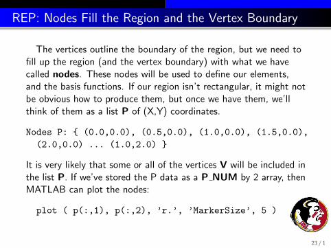
REP: Nodes Fill the Region and the Vertex Boundary

The vertices outline the boundary of the region, but we need tofill up the region (and the vertex boundary) with what we havecalled nodes. These nodes will be used to define our elements,and the basis functions. If our region isn’t rectangular, it might notbe obvious how to produce them, but once we have them, we’llthink of them as a list P of (X,Y) coordinates.

Nodes P: { (0.0,0.0), (0.5,0.0), (1.0,0.0), (1.5,0.0),

(2.0,0.0) ... (1.0,2.0) }

It is very likely that some or all of the vertices V will be included inthe list P. If we’ve stored the P data as a P NUM by 2 array, thenMATLAB can plot the nodes:

plot ( p(:,1), p(:,2), ’r.’, ’MarkerSize’, 5 )

23 / 1

REP: Triangles Are Formed From Nodes

Even if we can’t compute the triangles, we can imagine how tostore them. A triangle is formed by three nodes. We can store thecollection T of triangles as a T NUM by 3 array of node indices:

Triangles T: { (1, 2, 3), (6,1,4), (5,6,8), ...

... (89,43,27) }

When listing triangles, we choose the counterclockwise ordering.This means that every interior edge will be listed twice, whileboundary edges will all be listed once. In other words, the “logicalsum” of all the triangles is an outline of the original region!

MATLAB can plot a triangulation:

trimesh ( t, p(:,1), p(:,2) )

24 / 1

REP: The Node Boundary is Edges Used Once

One way to compute the node boundary takes all the edges anddrops the duplicates. The node boundary can be stored as aB NUM by 2 list of pairs of node indices:

Boundary Edges: { (1, 2), (7,18), (4,63), ... (82,14) }

Simply having a collection of boundary edges is different thanactually having the edges in sequence. If you need that, you startwith one edge, find a connecting edge, keep looking until you getback to where you started, and then check to see whether youhave more edges to work on.

We seem to have discussed the boundary twice. First was thevertex boundary, which only involved vertices. The node boundary,includes short line segments between nodes added to the boundarybetween the vertices.

25 / 1

REP: Triangle Neighbors

The standard finite element method doesn’t need to knowelement neighbors; however, there are many times when dealingwith a mesh when this is necessary. For example, there’s a fastalgorithm to find a random point hidden in one of 1,000,000elements that will take, on average, 500 trials, rather than 500,000,but it requires being able to move from one triangle to its neighbor.

All the information for determining triangle neighbors is available.Two triangles are neighbors if they share an edge. That is, onetriangle uses nodes 5 and 17, in that order, the other uses 17 and5. There are ways to efficiently examine all the edges, find thesepairs of matching data, and indicate that two triangles areneighbors. Some triangles don’t have a neighbor on a particularside, because they are on the boundary, so that neighbor is -1.

26 / 1

FEM Meshing




DISTMESH

MESH2D


Conclusion

27 / 1

DELAUNAY: Whence P and T?

A pair of mysteries remain:

where does the set of nodes P come from?

how are these nodes arranged into triangles T?

The answer to both questions involves the Delaunay triangulation,which can compute a “good” triangulation of any set of nodes P.

That explains T, but what about P? Well, it turns out that we canstart with an arbitrary or random set of nodes P, and useinformation from the Delaunay triangulation that will rearrange thenodes to better fill the region, either uniformly or in accordancewith some density function we specify. By iterating on this process,we get good nodes and good triangles.

28 / 1

DELAUNAY: A Maximal Triangulation

Suppose we generate a random set of nodes P within ourproblem region. We can then connect as many pairs of nodes aspossible without ever crossing a previous line. The result is a(maximal) triangulation of the nodes.

The process seems pretty arbitrary, and it fact there are manypossible triangulations of a set of points. You may wonder how toautomate this process; a natural way is to start by creating a gianttriangle that encloses all the points you are going to use.

Then add the first node. Connect it to each vertex of the enclosingtriangle, and you’ve got a maximal triangulation. Add the secondnode. It falls into one of the triangles you already created, so yousubdivide that triangle. Keep going. At the end, remove theenclosing triangle, and any edges that connect to it, and youhave a maximal triangulation of the nodes.

29 / 1

DELAUNAY: Sixteen Nodes to Triangulate

30 / 1

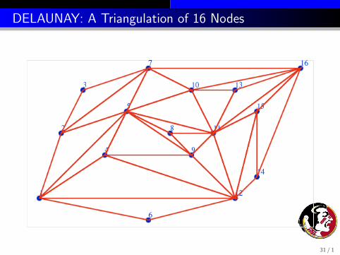
DELAUNAY: A Triangulation of 16 Nodes

31 / 1

DELAUNAY: What is a “good” triangulation?

We drew the lines of our triangulation at random. If we tried asecond time, we’d get a different picture. There are actually manyways to triangulate a set of points in the plane. Given that fact,it’s likely that some triangulations are “better” than others, butthat depends on what we want to do with our triangulations!

If we think about the connecting lines as “roads”, we might prefera triangulation that uses the shortest total length.

If we think about the triangles as representing patches of territory,we might dislike triangles that have a very small angle.

For graphics applications, and for many computational purposes,the avoidance of small angles is a very common criterion.

32 / 1

DELAUNAY: What is a “good” triangulation?

The Delaunay triangulation of a set of points is the (usuallyunique) triangulation which does the best job of avoiding smallangles.

Strictly speaking, we consider all possible triangulations of a set ofnodes. For each triangulation T , let θ(T ) be the smallest anglethat occurs in any triangle of that triangulation. Then atriangulation T ∗ is a Delaunay triangulation if

θ(T ) ≤ θ(T ∗)

for all triangulations T .

Since there are only finitely many possible triangulations, theDelaunay triangulation must exist, and if we had no other way,we could find it by computing and comparing every triangulation.

33 / 1

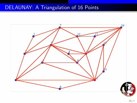
DELAUNAY: A Triangulation of 16 Points

34 / 1

DELAUNAY: A Delaunay Triangulation of 16 Points

35 / 1

DELAUNAY: A Delaunay Triangulation of 16 Points

Although we chose the Delaunay triangulation based on an angleconsideration, comparing the two pictures suggests that theDelaunay triangulation also does a better job of connecting nearbynodes rather than far-away ones, avoiding long triangle sides, andcreating triangles that have a more uniform shape.

The convergence of the finite element method come, in part, fromensuring that all the elements get small. The accuracy of the finiteelement calculations within a triangle depend, in part, on thetriangle having a relatively equilateral shape. The smoothness ofthe approximation depends somewhat on having relatively shorttriangle sides.

So the Delaunay triangulation has much to recommend it!

36 / 1

DELAUNAY: An Algorithm

Even though we will end up calling a piece of software to takecare of all the details for us, it’s important to understand thatthere are simple ways to compute a Delaunay triangulation.

For instance, a triangulation is Delaunay if each triangle is “locallyDelaunay”. A triangle is locally Delaunay if we can’t improve the(local) minimum angle by merging with a neighbor triangle andflipping the edge.

So we check each triangle, and if an edge swap improves the localminimum angle situation, we take it. We keep doing this until nomore improvement is possible.

It’s not magic, it’s an algorithm...

37 / 1

DELAUNAY: MATLAB Calculation

To compute the triangles that form a Delaunay triangulation ofa set of data points, use the MATLAB command

t = delaunay ( p(:,1), p(:,2) )

or

t = delaunayn ( p )

To display the triangulation,

t = delaunay ( p(:,1), p(:,2) )

triplot ( t, p(:,1), p(:,2) )

38 / 1

DELAUNAY: The C Program “Triangle”

Jonathan Shewchuk’s C program triangle triangulates a region,starting from a file containing the vertices of the boundary outline:

triangle -p v.poly

storing the nodes and triangles in new files.

It can use triangles no bigger than some limiting size:

triangle -a0.0015 v.poly

triangle is also available as a compiled library, which means a Cprogram you write can use triangle directly as it is running.

The home page is:

www.cs.cmu.edu/~quake/triangle.html

39 / 1

FEM Meshing




DISTMESH

MESH2D


Conclusion

40 / 1

DISTMESH: Using T to Improve P

So any set of nodes P defines a Delaunay triangulation T. Howcan we use T to improve P?

The meshing program distmesh(), by Persson and Strang, usesthe idea that, in the typical case, we’d like each node to be roughlythe same distance from all its neighbors. The Delaunaytriangulation connects a node to its neighbors (but not to far awaynodes!). We can imagine each of these connections to be a littlespring, which exerts a force if it is too long or too short.

So distmesh() actually sets up a linear system for the forces in adifferential equation, and then takes a small time step, that is, itlets each node respond to the force by moving in the appropriatedirection.

41 / 1

DISTMESH: Using T to Improve P

Once the nodes have been allowed to move, it is necessary torecalculate the spring forces, and take another step. By repeatingthis process carefully, a good result can be obtained.

Nodes that try to cross the boundary are pushed back in.

The result is a mesh of nodes that is well-spaced internally, andadapts to the shape of the boundary.

Moreover, if the user wants nodes to be denser in some areas thanothers, this information is easily used to make the springs “stiffer”in some regions and “looser” in others, again creating a mesh thatsmoothly varies in density according to the user’s request.

42 / 1

DISTMESH: Usage

[ p, t ] = distmesh ( @fd, @fh, h, box, itmax, fixed );

where:

@fd, the name of a distance function defining the region;

@fh, the name of a mesh density function;

h, the nominal mesh spacing;

box, a box that contains the region;

itmax, the maximum number of iterations;

fixed, a list of points which must be included;

p, node coordinates;

t, triangles defined by node indices.

43 / 1

DISTMESH: Region Defined by Signed Distance

A peculiar input to distmesh() is the distance function fd().This is the way the program expects the region to be defined. Thefunction returns a signed distance d from any point (x,y) to theboundary of the region, with the distance being negative if thepoint is actually inside the region.

This makes it wonderfully easy to describe mathematical regionssuch as a circle of radius r, because in that case

d =√x2 + y2 − r

However, for complicated geometries, it can be difficult to writedown a good formula, and inefficient for MATLAB to evaluate itmillions of times (which it must do!).

44 / 1

DISTMESH: The ELL Region

Although the L-shaped region is defined by straight linesegments, the true distance function is actually pretty complicated!

That is because exterior corners of the shape create curved levelsets of distance, while interior corners create sharp bends.

For convenience, distmesh() allows the user to define a distancefunction that is only approximate, but both the true distancefunction and the approximation can cause some odd behaviors inthe mesh near corners.

And trying to write an exactly correct distance function, even forthe L-shaped region, is surprisingly tricky!

Remind me to sketch the L-shaped distance function now!

45 / 1

DISTMESH: Distance function and Mesh for ”Holey Pie”

46 / 1

DISTMESH: The Same Ideas Work in 3D

47 / 1

DISTMESH: Reference

The source code for distmesh() is freely available at

http://persson.berkeley.edu/distmesh/

and a very readable and useful reference is available:

Per-Olof Persson, Gilbert Strang,

A Simple Mesh Generator in MATLAB,

SIAM Review,

Volume 46, Number 2, June 2004, pages 329-345.

http://persson.berkeley.edu/distmesh/persson04mesh.pdf

48 / 1

FEM Meshing




DISTMESH

MESH2D


Conclusion

49 / 1

MESH2D: Region Defined by Vertices

Darren Engwirda has adapted some of the ideas fromdistmesh() and added some new features that offer a secondpowerful and flexible MATLAB meshing program called mesh2d().

You can get a copy of mesh2d from the Matlab Central Exchange:

http://www.mathworks.com/matlabcentral/fileexchange/...

25555-mesh2d-automatic-mesh-generation

50 / 1

MESH2D: Usage

[ p, t ] = mesh2d ( vertices, edge, hdata, options );

where:

vertices, a V by 2 list of boundary vertex coordinates;

edge, (optional input), lists pairs of vertex indices that formthe boundary;

hdata, (optional input), a structure containing element sizeinformation;

options, (optional input), allows the user to modify thedefault behavior of the solver .

p, the coordinates of nodes generated by the program;

t, the triangulation of the nodes.

51 / 1

MESH2D: Usage

The mesh2d program has some nice features:

a very short call [p,t]=mesh2d(v) is possible;

short boundary segments result in small interior elements;

the region is described by vertices and the program isoptimized for this case; this means it’s actually pretty easy totriangulate a map, diagram, or CAD outline;

the output is “clean”; duplicate and unused nodes and smallelements are discarded, elements are in counterclockwiseorder.

a refine() function can refine a mesh.

a smoothmesh() function will smooth a mesh.

52 / 1

MESH2D: Simple ELL Mesh

As examples of mesh2d usage, we can start with variations ofthe L-shaped problem:

v = [ 0.0, 0.0; 2.0, 0.0; 2.0, 1.0; 1.0, 1.0; ...

1.0, 2.0; 0.0, 2.0 ];

[ p, t ] = mesh2d ( v );

http://people.sc.fsu.edu/∼jburkardt/m src/mesh2d/ell demo.m

53 / 1

MESH2D: Simple ELL Mesh

54 / 1

MESH2D: Two Short Boundary Segments

Suppose we add two extra boundary vertices:

v = [ 0.0, 0.0; 2.0, 0.0; 2.0, 0.25; 2.0, 0.5; ...

2.0, 1.0; 1.0, 1.0; 1.0, 2.0; 0.0, 2.0 ];

[ p, t ] = mesh2d ( v );

55 / 1

MESH2D: Two Short Boundary Segments

56 / 1

MESH2D: Set Maximum Element Size

Go back to the original problem, but specify a maximum elementsize:

v = [ 0.0, 0.0; 2.0, 0.0; 2.0, 1.0; 1.0, 1.0; ...

1.0, 2.0; 0.0, 2.0 ];

hdata = [];

hdata.hmax = 0.1;

[ p, t ] = mesh2d ( v, [], hdata );

57 / 1

MESH2D: Set Maximum Element Size

58 / 1

MESH2D: Use a Density Function

Go back to the original problem, but specify a density functionso elements are small near the reentrant corner:

v = [ 0.0, 0.0; 2.0, 0.0; 2.0, 1.0; 1.0, 1.0; ...

1.0, 2.0; 0.0, 2.0 ];

hdata = [];

hdata.fun = @hfun;

[ p, t ] = mesh2d ( v, [], hdata );

59 / 1


function h = hfun ( x, y )

%

% Minimum size is 0.01, increasing as we move away

% from ( 1.0, 1.0 ).

%

h = 0.01 + 0.1 * sqrt ( ( x-1.0 ).^2 + ( y-1.0 ).^2 );

return

end

60 / 1


61 / 1

MESH2D: Refine Example 1

Go back to the original problem, then refine the mesh:

v = [ 0.0, 0.0; 2.0, 0.0; 2.0, 1.0; 1.0, 1.0; ...

1.0, 2.0; 0.0, 2.0 ];

[ p, t ] = mesh2d ( v );

[ p, t ] = refine ( p, t );

62 / 1


63 / 1


64 / 1

MESH2D: Smooth Example 2

Go back to problem 2, but smooth the mesh:

v = [ 0.0, 0.0; 2.0, 0.0; 2.0, 0.25; 2.0, 0.5; ...

2.0, 1.0; 1.0, 1.0; 1.0, 2.0; 0.0, 2.0 ];

[ p, t ] = mesh2d ( v );

[ p, t ] = smoothmesh ( p, t );

65 / 1


66 / 1


67 / 1

FEM Meshing




DISTMESH

MESH2D


Conclusion

68 / 1

FILES: Compute Your Mesh Ahead of Time!

A person writing a finite element program does not need to dothe mesh generation inside the program! It is far better to takeadvantage of good software written by others.

The easiest way to handle this issue is to create the mesh ahead oftime, and write it to a file.

The triangle program automatically creates files of output.

distmesh() and mesh2d() can be convinced to do so.

Such files can be easily read back into a finite element programwritten in C, FORTRAN, PYTHON, or any appropriate language.

69 / 1

FILES: What a Node File Might Look Like

The fundamental mesh quantities are the arrays P and T, and ifwe understand them, we can handle other items, such as thetriangle neighbor list, or the boundary node list.

When dealing with communication between programs, the bestidea is to keep things simple. So we will create one file for eacharray. Text files are bigger, but easier to read than binary files.Since P is an array of P NUM rows by 2 columns, our file willcontain that many rows and columns of data.

The P file for the ell problem should look something like this:

0.0 0.0

1.0 0.0

2.0 0.0

... ...

2.0 4.0

70 / 1

FILES: What a Triangle File Might Look Like

Similarly there should be a separate T file, and because itcontains integers, we want to read and write it with an integerformat. (Note that the MATLAB save command writes integerswith a real number format that can cause problems later.)

The T file for the ell problem should look something like this:

1 2 6

7 6 2

2 3 7

8 7 3

.. .. ..

17 18 20

21 20 18

Any programming language should be able to read such files andstore the corresponding data.

71 / 1

FILES: A MATLAB Function To Write Integer Data

function triangle_write ( outfile, m, n, table )

outunit = fopen ( outfile, ’wt’ );

for j = 1 : n

for i = 1 : m

fprintf ( outunit, ’ %12d’, round ( table(i,j) ) );

end

fprintf ( outunit, ’\n’ );

end

fclose ( outunit );

return

end

http://people.sc.fsu.edu/∼jburkardt/m src/fem meshing/triangle write.m

72 / 1

FILES: The FEM Program Needs to Allocate Space

It’s a good idea to try to let the FEM program figure out thesize of the array simply by reading the file. That way, the sameprogram can solve problems of different sizes without needing tobe modified and recompiled.

It is not too difficult to write functions that will count the numberof lines in a file, and the number of data items on a single line.This gives you the number of rows and columns you need toallocate for your array.

But if you don’t like my idea, you can always put the number ofrows and columns as the first line of the file!

Once your FEM program knows how big the array is that isdescribed by the file, it can allocate the necessary space, and readthe actual data.

73 / 1

FILES: C++ Reads an MxN Integer Array

int **triangle_read ( string infile, int m, int n )

{

ifstream inunit;

int i, j;

int **t;

inunit.open ( infile.c_str ( ) );

t = i4mat_new ( m, n ); <-- Set up a two dimensional array t[][]

for ( i = 0; i < m; i++ )

{

for ( j = 0; j < n; j++ )

{

inunit >> t[i][j];

}

}

inunit.close ( );

return table;

}

http://people.sc.fsu.edu/∼jburkardt/m src/fem meshing/triangle read example.C

74 / 1

FILES: FORTRAN Reads an MxN Integer Array

subroutine triangle_read ( infile, m, n, t )

integer m, n

integer i

character ( len = * ) infile

integer t(m,n)

open ( unit = 1, file = infile, status = ’old’ )

do i = 1, m

read ( 1, * ) t(i,1:n)

end do

close ( unit = 1 )

return

end

http://people.sc.fsu.edu/∼jburkardt/m src/fem meshing/triangle read example.f90

75 / 1

FILES: Advantages to Using Files

When you let a program like mesh2d() create your finiteelement mesh, you get the advantage of being able to handlegeneral regions, variable size meshing, and so on.

But by storing your meshes as files, you also make it possible to

think about your FEM program independently of the mesh, sothat it can be written to solve any size or shape problem;

feed the mesh to different FEM programs, compare results;

compute a complicate mesh once, use it many times;

plot the mesh any time, without running the FEM program;

add/delete elements or nodes by (carefully) modifying files;

compute related quantities (such as the triangle neighbor list)by working directly on the files.

76 / 1

FEM Meshing




DISTMESH

MESH2D


Conclusion

77 / 1

CONCLUSION: The Whole Talk in One Slide

I have suggested that computing a good mesh for a big,interesting region is possible, important, but too hard for theaverage programmer to worry about.

There is good software available to carry out this task.

The meshing can be done in advance of the finite calculation, andthe mesh data stored as files in a simple way.

I’ve suggested some MATLAB software that is easy to use.

Since graphical output can be crucial for checking a mesh, I’veoutlined some procedures for displaying mesh data.

78 / 1

CONCLUSION: Things I Skipped

I concentrated on the MATLAB programs distmesh andmesh2d because they are accessible, powerful, usable, and easy todisplay graphically.

There are many other packages available. I only briefly discussedtriangle, but for many computational tasks it might be a verygood choice for you, particularly because it can be incorporatedinto a larger C program you write.

I showed some surfaces with meshes, and some 3D objects thatwere meshed, but I only hinted at how these things can be created.You should imagine that these problems are related to the simplerthings we talked about. If they interest you, you can find out theirrelation to the simple programs and problems we looked at.

79 / 1

CONCLUSION: Your Future in Meshing

While we have encountered meshing from a finite elementapproach, it’s really a fundamental operation of computationalscience, coming up whenever a geometric object needs to berepresented, analyzed, and manipulated.

This means understanding meshing gives you an opening into

computer graphics, 3D animation, gaming;

computer geometry;

facial recognition;

GIS (geographic information systems);

medical scan analysis;

CAD/CAM, (computer-aided design and modeling);

3D “printers”.

In other words, while it’s possible that your future will involveworking with finite elements, it’s certain that you will be workingwith meshes. Learn to love them!

80 / 1

Meshing for the Finite Element Method -...

Documents

Transcript of Meshing for the Finite Element Method -...