Mergers and Acquisitions FINC3013 – Valuation in an M&A context Angelo Aspris.
Mergers and Acquisitions and the Valuation of Firms
Marcelo Bianconi, Tufts University* Chih Ming Tan, University of North Dakota Yuan Wang, Tufts University Joe Akira Yoshino, FEA-Ecconomics-USP
Abstract
We use EV/EBITDA as a measure of firm value and the financial fundamental ratios price to sales ratio, debt to equity ratio, market to book ratio and financial leverage as controls to measure the effect of mergers and acquisitions (M&A) on firm value. We use a large panel of 65,000 M&A deals globally from the Communications, Technology, Energy and Utilities sectors between the years of 2000 to 2010. First, we find significant contemporaneous effects of the financial fundamental ratios on firm value. Second, we find evidence of negative long-term M&A effects and positive instantaneous M&A impact on firm value because EV moves faster relative to a slow moving EBITDA. Finally, we find that the effect of M&A on firm value in the financial crisis of 2008 is much distinct from the same effect during the recession of 2001. Keywords: Mergers and acquisitions (M&A), firm value, EV/EBITDA, treatment effect, DID estimation, propensity score matching JEL Classification Codes: G34, C31, C33 Contact: * Bianconi: Professor of Economics, [email protected] Preliminary, October 2014 Comments Welcome We thank Dan Richards for helpful comments and Tufts University for use of the High-Performance Computing Research Cluster. Any errors are our own. ______________________________________________________________________________
2
1. Introduction
Mergers and acquisitions (M&A) is a general term used to refer to the consolidation of
companies. It is part of corporate strategy, corporate finance and management dealing with the
buying, selling, dividing, spinning and combining of different companies and similar entities that
can help an enterprise grow rapidly in its sector or location of origin, or a new field or new
location, without creating a subsidiary, other new entity or using a joint venture. A merger is a
combination of two companies to form a new one, while an acquisition is the purchase of one
company by another in which no new company is formed. Either structure can result in the
economic and financial consolidation of two entities.
Historically, we can identify roughly six waves of M&A activities. The first wave of
horizontal mergers in 1897-1904; the second wave of vertical mergers in 1916-1929; the third
wave of diversified conglomerate mergers in 1965-1969; the fourth wave of congeneric mergers,
hostile takeovers and corporate raiding in 1981-1989; the fifth wave of cross-border mergers in
1992-2000; and the sixth wave of shareholder activism, private equity and leveraged buyout
(LBO) in 2003-2008.
M&A activity may also be construed as a type of restructuring in some entity
reorganization with the aim of providing growth and value. Consolidation of an industry or
sector occurs when widespread M&A activities concentrate the resources of many small
companies into a few larger ones. For example, a large wave of M&A deals occurred in the
automotive industry in the U.S. between 1910 and 1940, and a turbulent time for the airlines
M&A was between 1970's and 1980's. Most importantly, the great revolution of information and
telecommunications between 1985 and 2000 pushed global M&A activities in the technology
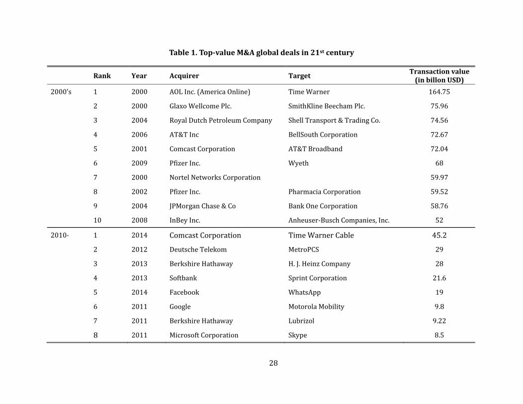
and communication sectors to hit a highest level in the 21st century. In the beginning of 2014,
Comcast Corporation and Time Warner Cable engaged in a friendly merger thus creating a
world-wide technology and media company. The agreement is stock-for-stock transaction in
which Comcast would acquire 100 percent of Time Warner Cable’s 284.9 million shares
outstanding for shares of CMCSA amounting to approximately $45.2 billion in equity value in
February of 2014. Also, Facebook announced in February 2014 that it had reached a definitive
agreement to acquire WhatsApp, a rapidly growing cross-platform mobile messaging company,
for a total of approximately $19 billion, including $4 billion in cash, approximately $12 billion
3
worth of Facebook shares and additional $3 billion in restricted stock units to be granted to
WhatsApp’s founders and employees that will vest over four years subsequent to closing. So far
during 2014, the worldwide mergers and acquisitions transaction value in the technology sector
soared to $65.2 billion, up 90% from the same period last year which was US$34.4 billion and
the highest year-to-date level since 2000. The top-value global M&A deals in all sectors are
listed in Table 1.
Ultimately, our literature review shows that there is no agreement on either the motives
or the effects of M&A on firm performance. Our aim is to measure the effect of M&A activities
on firm value. We choose an enterprise value multiple as the metric for firm value since it takes
debt into account, which the acquirer will have to assume, and eliminates the potential influence
of inflation and tax policy. Thus, we can compare the results on firm value across countries and
across time periods.
In particular, we investigate whether or not M&A have an impact on firm value; which
factors have a significant effect, and how they influence firm value instantaneously and in the
long-run. Moreover, an enterprise multiple may vary depending on the industry type. We
examine the Communications, Technology, Energy and Utilities sectors, in order to understand
the differences in technology-intensive and resource-intensive firms. We use a large sample
consisting of global M&A deals for the period between the year of 2000 and 2010, using fixed-
effects, dynamic panel regression and treatment effect models including propensity score
matching with differences-in-differences. Table 2 presents a classification of the sectors and
subsectors examined in this paper.
The paper is organized as follows. First, we present an introduction followed by a
literature review. Section 3 then outlines the definition and descriptive statistics of the variables
in sample dataset. Section 4 provides the empirical models and estimations including
contemporary impact on firm value from financial fundamental ratios by panel regressions, the
instantaneous, long-term effect and difference-in-differences estimations of M&A activities on
firm values. Section 5 summarizes the major findings and gives recommendations for future
research work.
4
2. Literature review
The magnitude of M&A phenomena has raised questions related to why M&A occur and how
M&A affect the outcome of corporations in terms of financial performance, research and
development, productivity and market share. Since the late 1990s, the literature focused on the
theory of mergers and acquisitions, providing insights into the success or failure of M&A
activities. The issues ranged from theories of the firm conceptualized into the motives for merger,
their empirical investigation, performance measurement of merged firms using share price data
and accounting data, empirical examination of financial characteristics of acquirer and target
firms and the determinants of aggregate merger activity. Despite the large literature, there is no
agreement about either the motives or the effects of M&A (Chapman 2003, Chen and Findlay
2003, DeYoung et al. 2009, Kwoka 2002, Menapara and Pithadia 2012, Schulz 2007).
A key main motivation for M&A is to provide growth of the company or positive
shareholder value. The general motivations come from financial performance, technology
innovation and market trend. The acquiring firm seeks improved financial performance (Erel et
al. 2012). A more traditional view is that M&A take place to lower the costs of the company
relative to the same revenue stream and increase profit margins, thus maximizing stockholder
wealth (Bradley et al. 1988, Manne 1965). The acquisitions serve as a means to seize the
efficiency gain potentially stemming from economies of scale and scope, managerial and
financial synergies, and superior management. Also, a company is more competitive as it
increases its market share. The acquirer firm can obtain a group of target markets for actual and
potential products to be sold in those markets; meanwhile it absorbs a major competitor and thus
increases its market power by capturing increased market share to set prices (Abellán 2004).
Moreover, many M&A activities provide an opportunity for corporations and their shareholders
to receive some tax benefits, in a small minority of cases these benefits are larger in comparison
to the value of the acquired company, suggesting tax provided motivation. But, even in cases
where there are significant tax benefits, there is no strong evidence that they were the driving
factors in the takeovers (Auerbach and Reishus 1987). On average and across the most
commonly studied variables, acquiring firms' financial performance does not positively change
as a function of their acquisition activity (King et al. 2004). M&A activities appear to occur in
different extents across different sectors. In technology-intensive firms (i.e. Communications and
5
Technology sectors), M&A appears to be strongly associated with R&D intensity and
innovation. Due to fast growing technological change, an acquirer can take advances of a target’s
product capability, patents and brand recognition by their customers (Sevilir and Tian 2012). The
transfer of technologies and capabilities results in faster growth of acquirers (Ranft and Lord
2002). More recent literature also suggests that corporate managers conduct M&A to expand the
power of their companies so as to facilitate their empire-building (Ravenscraft and Scherer
1987).
In the resource-intensive firms (i.e. Energy sector and Utilities sector) the focus is on
geographical expansion, resource transfer and diversification. A non-financial merger motivator
has long been believed to be geographic diversification. It is an attempt to expand market share,
decrease risk, and in the long run increase profits (Frohlich and Kavan 2000). Many others
(Baker et al. 1988, Conyon and Gregg 1994, Firth 1991) find that executive rewards increase
with firm size in the wake of acquisitions. Also, resource and nonperforming assets are unevenly
distributed across firms (Barney 1991) and the interaction of target and acquiring firm resources
can create value through either overcoming asymmetry or by combining scarce resources (King
et al. 2008).
Besides the motivations from the company’s perspective, the boom in M&A is also a
general phenomenon generated by new global conditions, such as trends linked to the
transformation of markets, e.g. the flourishing of regulatory shifts; and technology, e.g. the
emergence of new business and market opportunities, the rise of technological interrelatedness,
and the establishment of new communications and cross-border restructuring (Cassiman and
Colombo 2006).
In terms of M&A effects, they have been used as instruments for firm growth for many
years. Engaging in M&A represents an important commitment for any company as it affects
every facet of its organization. Studies of this approach for emerging markets like China and
India were undertaken in Menapara and Pithadia (2012), and cross-border M&A deals were
examined in Chapman (2003), Chen and Findlay (2003) and Jongwanich et al. (2013). In order to
best measure pre- and post- M&A effects, we can examine synergy realization, absolute
performance, and relative performance. Analytical methods include, but are not limited to, mean
and standard deviation, ratio analysis, paired sample t-test, which involves the use of accounting

6
measures like size, growth, profitability, risk and leverage to analyze the performance
characteristics of the acquirer and target (merging and merged) firms in the pre- and post-
takeovers periods (Vanitha and Selvam 2007); and difference-in-difference estimation to single
out the causal effect of M&A (Hall 1990, Szücs 2013).
The economic advantages of M&A have been examined at length. Caves (1989) and
Röller et al. (2000) provided support for the thesis that firms achieve or strengthen market power
and obtain efficiency gains by being able to exploit economies of scale and scope. Kumar and
Singh (1994)’s case study concluded that rehabilitation of a sick company by merging with a
healthy company is one of the most effective way for their rehabilitation. Sanker and Rao (1998)
analyzed the implications of takeovers from the financial point of view with the help of certain
parameters like liquidity, leverage and profitability. They observed that a sick company is taken
over by a good manager and makes serious attempts to turnaround successfully. Pawaskar (2001)
compared the pre- and post- merger operating performance of the corporations involved in
merger between 1992 and 1995 to identify their financial characteristics; this study identified the
profile of the profits and showed that the merging firms were at the lower end in terms of growth,
tax and liquidity of the industry, while the merged firms performed better than the respective
industry in terms of profitability. Saple (2000) also found that the target firms were better than
industry averages while the acquiring firm had lower than industry average profitability.
Agrawal and Jaffe (2000) brought out “The Post-merger Performance Puzzle.” They
examined the literature on long-run abnormal returns following mergers, and also examined
explanations for any findings of underperformance following mergers; they concluded that the
evidence does not support the conjecture that underperformance is specifically due to a slow
adjustment to merger news, and rejected the earnings-per-share myopia hypothesis, i.e. the
hypothesis that the market initially overvalues acquirers if the acquisition increases EPS,
ultimately leading to long-run under-performance. The success of merger and acquisitions
depends on proper integration of employees, organization culture, IT, products, operations and
service of both the companies. Proper integration in mergers plays a critical role in determining
how effectively merged organizations are able to integrate business processes and people, and
deliver products and services to both internal and external customers of the organization.
7
Nevertheless, despite the many advantages M&A could offer, the statistical evidence
supporting the hypothesis that profitability and efficiency increase following M&A is at best
weak (Berkovitch and Narayanan 1993, Jensen and Ruback 1983, Lichtenberg 1992, Mueller
1980, Ravenscraft and Scherer 1987). The problem with most existing studies is that they
disregard the issue on how value is created through M&A and hence fail to identify the
conditions that should hold for M&A to positively contribute to firm’s performances (Caves
1989).
Some notable and seminal empirical studies show a negative impact of M&A on the
financial and economic performance of companies. Vanitha and Selvam (2007) analyzed the pre-
and post- merger financial performance of manufacturing sector during 2000-2002; they found
that the overall financial performance of merged companies in respect of 13 variables were not
significantly different from the expectations. Mantravadi and Reddy (2007, 2008) conducted
research to study the impact of M&A on the operating performance of the acquiring corporation
in different periods in India, by examining some pre- and post- merger financial ratios with
chosen sample firms and mergers between 1991-2003. Their results suggest that there are minor
variations in terms of impact on operating performance following merger in different intervals of
time in India. Kumar (2009) also examined the post-merger operating performance of a sample
of 30 acquiring companies involved in merger activities during 1999-2002 in India; the study
attempted to identify synergies, if any, resulting from mergers and found that post-merger
profitability, asset turnover and solvency of the acquiring companies, on average, showed no
improvement when compared with pre- merger values. Other studies link M&A and R&D (Hall
1990). Hitt et al. (1991) and (1996) find that M&A seem to shift the innovative strategy more
towards external sourcing. Szücs (2013) used different matching techniques to construct separate
control groups for acquirers and targets to single out the causal effect of mergers on R&D growth
and intensity. They found that M&A have a direct significant negative impact on internal R&D
inputs, as well as ex-post R&D output compared to competitors.
Despite the goal of performance improvement, results from mergers and acquisition are
sometimes disappointing compared with what is predicted or expected. Numerous empirical
studies show high failure rates of M&A deals. They develop a comprehensive research
framework that bridge different perspectives and promote understanding of factors underlying

8
M&A performance in business research and scholarship (Straub 2007). As Barnes said,
“Although some regions present access to new consumer populations and additional growth
opportunities exist in other fast-growing emerging markets, investors are playing it safe by
staying on the sidelines to avoid the risks associated with expanding their organizations’ global
footprint.” These studies should help managers in the decision making and M&A process.
In this paper, we measure the effect of M&A activities on firm value using an enterprise
value multiple as the metric for firm value. We examine whether or not mergers and acquisitions
have an impact on firm value; which factors have a significant effect, and how they influence
firm value instantaneously and in the long-run. Moreover, an enterprise multiple may vary
depending on the industry type. We examine the Communications, Technology, Energy and
Utilities sectors, in order to understand the differences in technology-intensive and resource-
intensive firms. We use a large sample consisting of global M&A deals for the period between
the year of 2000 and 2010, using fixed-effects, dynamic panel regression and treatment effect
models including propensity score matching with differences-in-differences.
3. Data and Descriptive Statistics
The sample of firm-level financial data was collected from the Bloomberg database. We looked
for the firms worldwide with M&A completed activities during the year of 2000 to 2010, and the
deals were both domestic and cross-border. For each deal, we focused on the acquirer firm’s
financial fundamental data for a time period of seven years: three-years before the M&A, one-
year when M&A takes place and three-years after the M&A takes place thus yielding a balanced
panel dataset.
We include five financial fundamental ratios as measurement and controls in the models:
enterprise multiple, price to sales ratio, debt to equity ratio, market to book ratio and financial
leverage.1 Enterprise value (EV) is an economic measure reflecting the market value of a whole
business. Enterprise value is calculated as market capitalization plus debt (both long-term and
short-term), minority interest and preferred shares, minus total cash and cash equivalents. It is
1ThedefinitionsandinterpretationsofthesevariablesandacompletelistoftermsdescribingM&AactivityareavailableinanAppendixuponrequest.
9
more comprehensive than market capitalization, which only includes common equity. Enterprise
value differs significantly from simple market capitalization in several ways, and many consider
it to be a more accurate representation of a firm's value. One may think of enterprise value as the
theoretical takeover price. In the event of a buyout, an acquirer would have to take on the target’s
debt, but would pocket its cash. The value of a firm's debt would need to be paid by the buyer
when taking over a company, thus EV provides a much more accurate takeover valuation
because it includes debt in its value calculation.
Earnings before interest, taxes, depreciation and amortization (EBITDA) is an indicator
of a company's financial performance. It is computed by revenue minus expenses (excluding
interest, taxes, depreciation and amortization). EBITDA is essentially net income with interest,
taxes, depreciation and amortization added back to it, and can be used to analyze and compare
profitability between companies and industries because it eliminates the effects of financing and
accounting decisions. Many companies, especially in the technology sector, now commonly
quote it. EBITDA gives a good metric to evaluate a business’ current operational profitability,
but not cash flow. It also leaves out the cash required to fund working capital and the
replacement of old equipment, which can be significant. Although EBITDA is not a financial
metric recognized in generally accepted accounting principles, it is widely used when assessing
the performance of companies. It is intended to allow a comparison of profitability between
different companies, by canceling the effects of interest payments from different forms of
financing (by ignoring interest payments), political jurisdictions (by ignoring tax), collections of
assets (by ignoring depreciation of assets), and different takeover histories (by ignoring
amortization).
A negative EBITDA indicates that a business has fundamental problems with
profitability. A positive EBITDA, on the other hand, does not necessarily mean that the business
generates cash. This is because EBITDA ignores changes in working capital (usually needed
when growing a business), capital expenditures (needed to replace assets that have broken down),
taxes, and interest.
Enterprise multiple (EV/EBITDA) is a ratio used to determine the value of a company. It
is calculated as enterprise value divided by its earnings. It’s useful for transnational comparisons
because it ignores the distorting effects of individual countries' taxation policies. Enterprise

10
multiples can vary depending on the industry. It’s important to compare the multiple to other
companies or to the industry in general. Expect higher enterprise multiples in high growth
industries (like biotech) and lower multiples in industries with slow growth (like railways). The
EV/EBITDA multiple is a better metric than market capitalization for takeovers. It looks at a
firm as a potential acquirer would, and used to find attractive takeover candidates. Compared to
other multiples like the P/E, this ratio may be preferred because it is normalized for differences
between companies: using EBITDA normalizes for differences in capital structure, taxation and
fixed asset accounting; meanwhile, using enterprise value also normalizes for differences in a
company's capital structure. A company with a low enterprise multiple might be undervalued,
and thus can be viewed as a good takeover candidate.
Broadly speaking, a company's assets are financed by either debt or equity. The weighted
average cost of capital (WACC) is the rate that a company is expected to pay on average to all its
security holders to finance its assets. The inverse of enterprise multiple, EBITDA/EV, is also a
financial ratio that measures a company's return on investment. The company directors can
compare their return with how much interest they have to pay for every dollar it finances, then
determine the economic feasibility of expansionary opportunities and mergers.
Price to sales ratio (P/S) is a valuation ratio that compares a company’s stock price to its
revenues. It is an indicator of the value placed on each dollar of a company’s sales or revenues.
This ratio can be calculated either by dividing the company’s market capitalization by its total
sales over a 12-month period, or on a per-share basis by dividing the stock price by sales per
share for a 12-month period. Like all ratios, the price-to-sales ratio varies greatly from sector to
sector, so it is most relevant when used to compare companies within the same sector. A low
ratio may indicate possible undervaluation, while a ratio that is significantly above the average
may suggest overvaluation.
The smaller this ratio is (i.e. less than 1.0), signals a better investment opportunity since
the investor is paying less for each unit of sales. But investors should exercise caution when
using price to sales ratios since the numerator, the price of equity, takes a firm's leverage into
account, whereas the denominator, sales, does not. Comparing P/S ratios carries the implicit
assumption that all firms in the comparison have an identical capital structure. This is always a
problematic assumption, and even more so when the assumption is made between industries,

11
since industries often have vastly different typical capital structures (for example, a technology
vs. a utilities company). This is the reason why P/S ratios across industries vary widely.
Debt to equity ratio (D/E) is a measure of a company's financial leverage calculated by
dividing its total liabilities by stockholders' equity. It also depends on the industry in which the
company operates. For example, capital-intensive industries tend to have a D/E ratio above 2,
while technology-intensive companies have a D/E ratio of under 0.5. Debt to equity ratio
indicates what proportion of shareholders’ equity and debt a company is using to finance its
assets. A high D/E ratio generally means that a company has been aggressive in financing its
growth with debt, i.e. the company could potentially generate more earnings than it would have
without this outside financing. But this can result in volatile earnings as a result of the additional
interest expense. If this were to increase earnings by a greater amount than the debt cost
(interest), then the shareholders benefit as more earnings are being spread among the same
amount of shareholders. However, the cost of this debt financing may outweigh the return that
the company generates on the debt through investment and business activities and become too
much for the company to handle. This can lead to bankruptcy, which would leave shareholders
with nothing.
Market-to-book ratio (M/B) is a financial ratio used to find the value of a company by
comparing the current market value of a firm to its book value. Market value is determined in the
stock market through its market capitalization. Book value is calculated by looking at the firm's
historical cost, or accounting value. The ratio can be calculated in two ways, either divide the
company's market capitalization by its total book value, or use the book value per-share to divide
the company's current share price, but the result should be the same in each way. As with most
ratios, it varies a fair amount by industry. Industries that require more infrastructure capital (e.g.
Utilities firms) will usually trade at P/B ratios much lower than, for example, technology firms.
This ratio attempts to identify overvalued or undervalued securities by taking the market
value and dividing it by book value. In basic terms, if the ratio is above 1 then the stock is
overvalued; if it is less than 1, the stock is undervalued. A higher M/B ratio implies that
investors expect management to create more value from a given set of assets, all else equal. M/B
ratios do not, however, directly provide any information on the ability of the firm to generate
profits or cash for shareholders.
12
Financial leverage is the degree to which a company uses fixed-income securities such as
debt and preferred equity. The more debt financing a company uses, the higher its financial
leverage. A high degree of financial leverage means high interest payments, which negatively
affect the company's bottom-line earnings per share. Businesses leverage their operations by
using fixed cost inputs when revenues are expected to be variable. An increase in revenue will
result in a larger increase in operating income. Financial leverage can be calculated by the ratio
of total assets to shareholders’ equity, or equivalent to a ratio of return on equity to return on
assets. In corporate finance, operating leverage is an attempt to estimate the percentage change
in operating income for a one-percent change in revenue, and financial leverage tries to estimate
the percentage change in net income for a one-percent change in operating income; the product
of the two is called total leverage and estimates the percentage change in net income for a one-
percent change in revenue.
While leverage magnifies profits when the returns from the asset more than offset the
costs of borrowing, losses are magnified when the opposite is true. A corporation that borrows
too much money might face bankruptcy or default during a business downturn, while a less-
levered corporation might survive. So while adding leverage to a given asset always adds risk, it
is not the case that a levered company or investment is always riskier than an unlevered one. In
fact, many highly levered hedge funds have less return volatility than unlevered bond funds
and public utilities with lots of debt are usually less risky stocks than
unlevered technology companies. The financial crisis of 2007–2009, like many previous
financial crises, was blamed in part on excessive leverage.
3.1 Descriptive statistics
We collect data of firms worldwide from four sectors, e.g. Communication, Technology, Energy
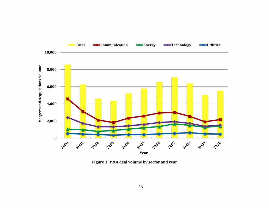
and Utilities, who have M&A activities during the year of 2000 to 2010. In Table 3, the total
volume of M&A activities per year within these four sectors varied between 4,000 and 9,000 for
the first 10 years of 21th century. The cyclical nature of the market and the economy suggests
that every strong economic growth bull market in history has been followed by a sluggish low
growth bear market. As shown in Figure 1, the trend of the number of M&A deals follows the
macroeconomic cycle in general, the largest amount of deals was observed in the year 2000,
followed by a fast decline during the trough years of 2001 to 2003. As financial markets turn
13
better, the number of deals climb from approximately 2004 and kept increasing to another peak
in 2007. After the subprime crisis of 2008, the number of deals falls through 2010.
Comparing the four sectors, more M&A deals emerge in the Communications sector
followed by the Technology sector and the trend follows the macroeconomic cycle closely. In
the resource-intensive industries of Energy and Utilities, we observe less M&A activity, and it
does not cycle closely with the market. This is because Communications and other service
sectors are most involved in the major change of liberalization in international capital
movements and investments. Regulatory reforms in these sectors are playing an important role in
the dramatic increase in M&A. Also, the pace of technological change has generated new
business and markets. Due to the time and cost constraints, companies may experience
difficulties in developing in-house R&D, so they may opt for M&A as a means of acquiring
technological and human resources in order to remain internationally competitive. The drastic
decline in communications and transportation costs has also been identified as a major factor
behind the latest M&A wave.
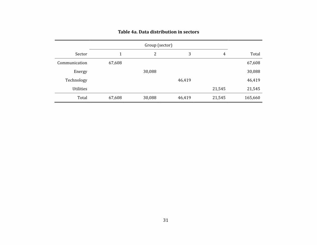
Our sample includes 65,521 firms with 458,647 observations in total. We analyze the
firm’s enterprise multiple EV/EBITDA for a period of seven years and the effect of M&A
activities on firm value. To reduce the weight of outliers, we censor the dependent variable,
EV/EBITDA, at the 1st and 99th percentiles by setting extreme values to the 1st and 99th percentile
values, respectively. The M&A deals which have only one year of data available were also
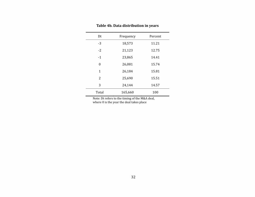
eliminated from the panel. As a result, the unbalanced panel dataset consists of 31,284 M&A
deals with 165,660 observations: 67,608 from Communication sector, 46,419 from Technology
sector, 30,088 from Energy sector and 21,545 from Utilities sector; the time dimension is evenly
distributed in seven years, as listed in Table 4a and 4b.
Besides the EV/EBITDA multiple, several firm financial fundamental ratios are included
as control variables, e.g. price to sale ratio (P/S), debt to equity ratio (D/E), market to book ratio
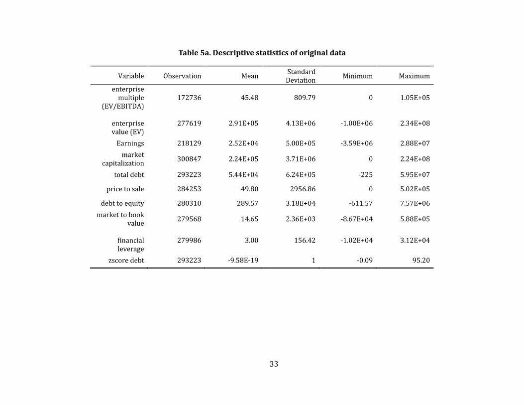
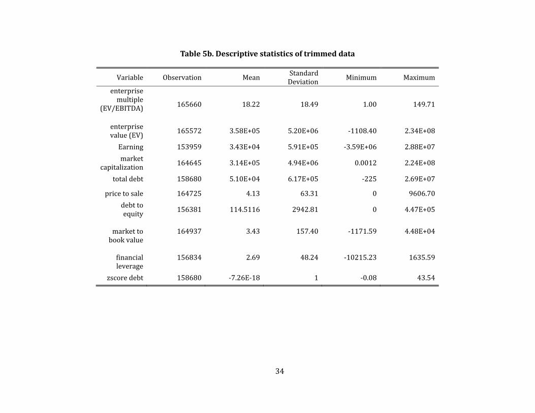
(M/B) and financial leverage (FL). The descriptive statistics of raw and trimmed data are
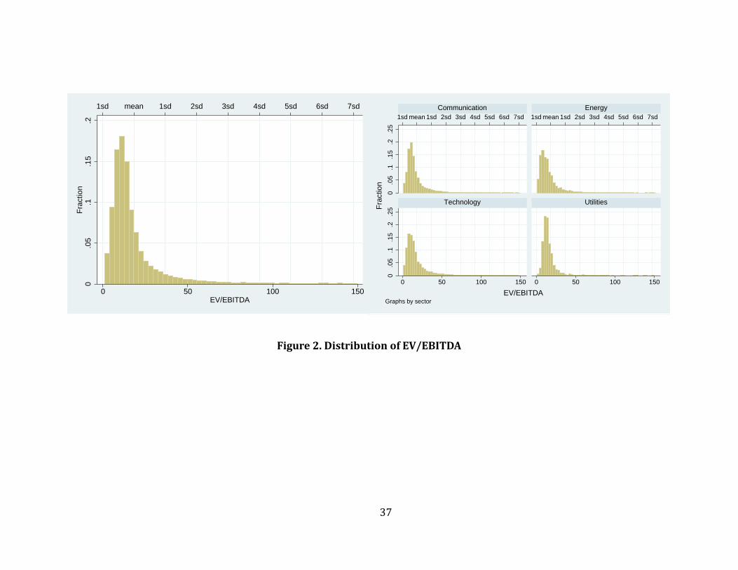
summarized in Table 5a and 5b. First, we note that the enterprise value multiple is in the range of
1 to 150 with mean of 18.22 and standard deviation 18.49 and Figure 2 presents the distribution
of EV/EBITDA, and by sector. The average P/S ratio is 4.13, the average D/E ratio is 114.51, the
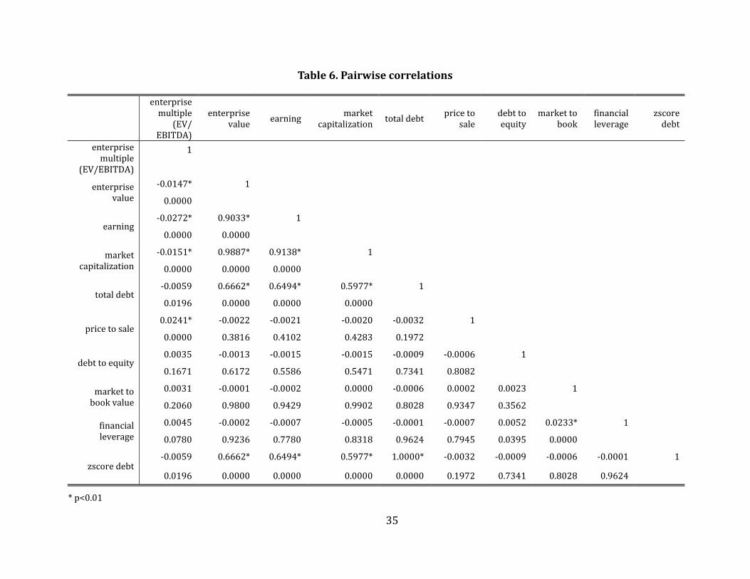
average M/B ratio is 3.43 and average FL is 2.69. We also note in Table 6 that the unconditional

14
correlation between EV/EBITDA and short- and long-term debt is significant at the 5% level,
thus we take total debt into account after normalization (zscore). We also present pair-wise
correlations between the five control variables; they are not correlated at 1% significant level,
except for financial leverage and market to book ratio.
4. Econometric Models and Empirical Results
We present the several econometric models and estimation in the following.
4.1 Panel Fixed Effects and Dynamic Panel Models
First, we estimate two econometric models: panel fixed effects and Arellano and Bond dynamic
panel methodology. The panel fixed effects model is given by
. (1)
We also use the Arellano and Bond dynamic panel estimations since we have a small number of
years and a large number of firms, and the dynamic panel model is given by
. (2)
In the models above, i indexes the firm and t indexes the relative year to the mergers and
acquisitions activity. The main hypotheses refer to the signs and magnitudes of the
coefficients . The models are first applied to all observations in the panel dataset, and
specifications refer to overall effects on firm valuation. Second, we estimate those regressions
for each sector separately and also on every year to capture the effect in specific industry and
time periods.
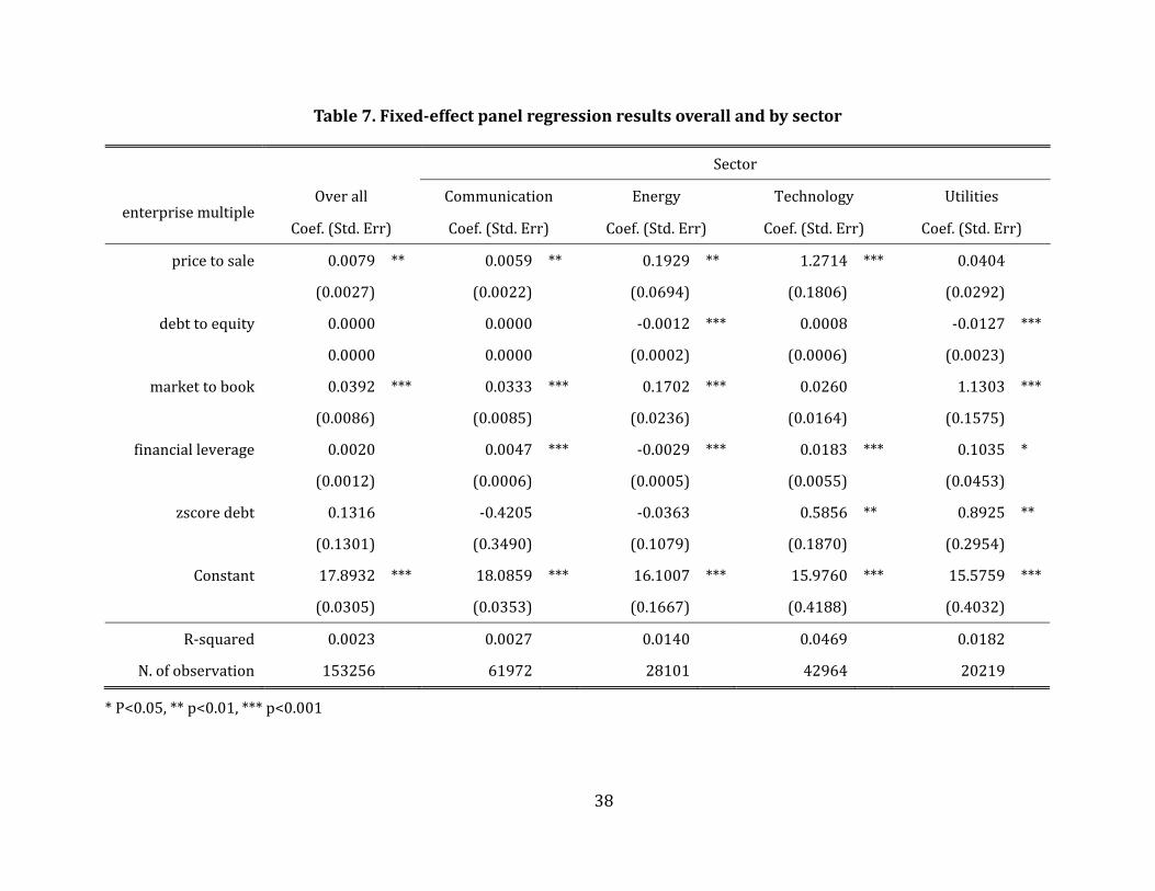
The results of fixed-effect panel regressions are list in Table 7. Column 1 refers to the
relationship between firm’s enterprise multiple (EV/EBITDA) and its financial fundamental ratios
(P/S, D/E, M/B, FL and ZD). This regression includes firms in all four sectors. The first main
result is that the price to sales ratio and market to book ratio have significant positive effects on
enterprise multiple, while debt to equity ratio and financial leverage are statistically insignificant
to firm value. An increase of one unit in price to sales ratio and market to book ratio brings up
the enterprise multiple on average by 1% and 4%, respectively; because market capitalization is

15
positive related to EV. Columns 2 to 5 present the regression results for each one of those four
sectors, Communication, Technology, Energy and Utilities, to capture the industry type effects.
The main results of columns 1 continue to hold. Now, the financial leverage has a significant
positive effect on firm value of Communication and Technology companies, while this effect is
negative on Energy firms. Also, total debt to equity ratio affects firm values only in Energy and
Utilities sectors. An increase of one unit in debt to equity ratio lower the enterprise multiple by
1‰-1%, since short- and long-term debt is negative related to EV.
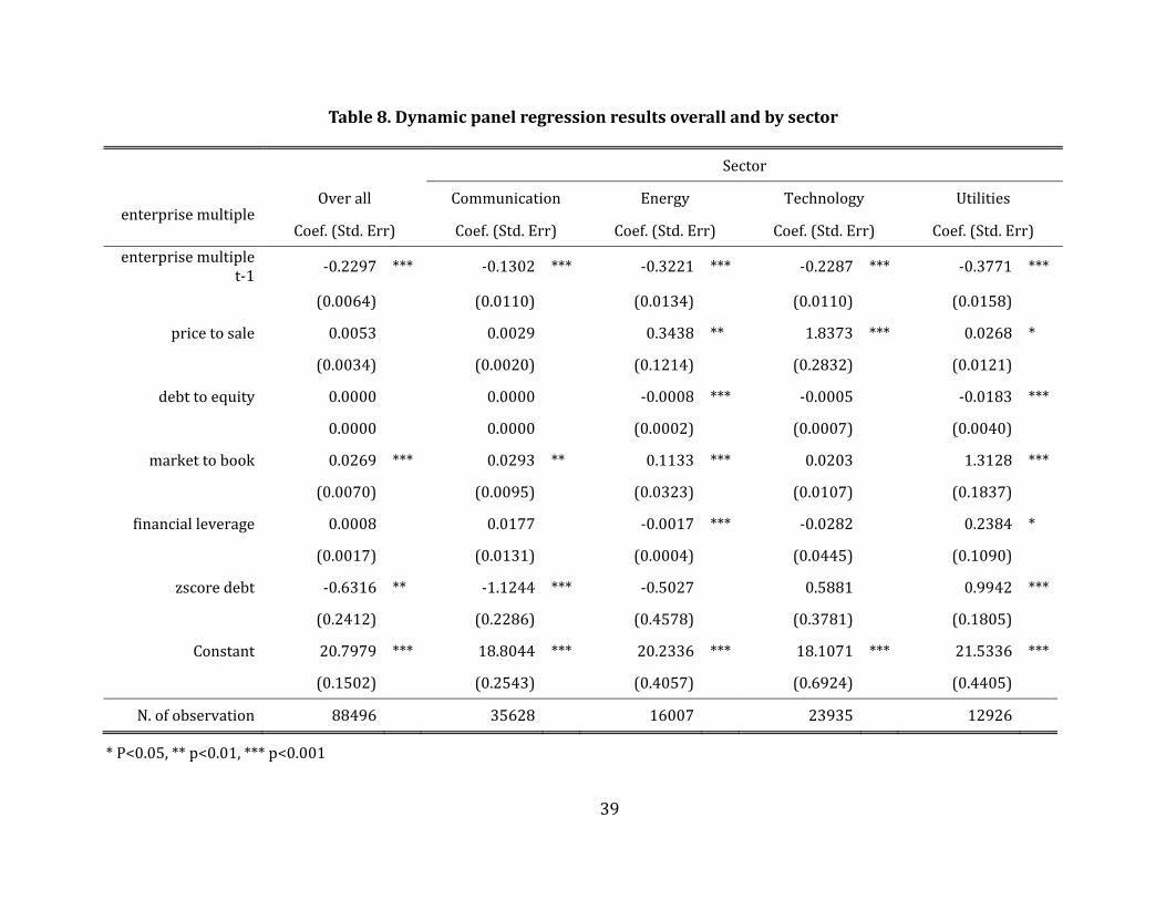
The dynamic effects come next. Besides all the contemporary financial fundamental
ratios list above, we believe that the firms’ current value should be also highly related to their
performance in the previous years. 2 We estimate the Arellano and Bond dynamic panel
regression including one-lag of EV/EBITDA in the model. As shown in Table 8, the coefficient
on EV/EBITDAt-1 is highly significant; and it indicates negative autocorrelation. The magnitude
is large, about -23% in this dynamic model, indicating potential for overreaction and under-
reaction of EV/EBITDA over time. This dynamic effect is well identified in all sectors examined.
In column 1 of Table 8, the effects of the independent variables are similar to the fixed-effect
model shown in Table 7, which indicates a robust impact of financial ratios on firm value.
However, in columns 2 to 5, we find some changes in the result of dynamic panel model for each
sector. In the Communications and Technology sectors, the contemporary effect of financial
leverage in the dynamic model is not significant as well as the price to sale ratio in the
Communications sector. The effect of the market to book ratio is still highly significant, but with
lower magnitudes.
Overall, in Table 8 we find consistent and robust evidence that current firm values are
much sensitive to the lagged values. The market to book ratio is a robust factor across all sectors,
while others are not significant in all cases.
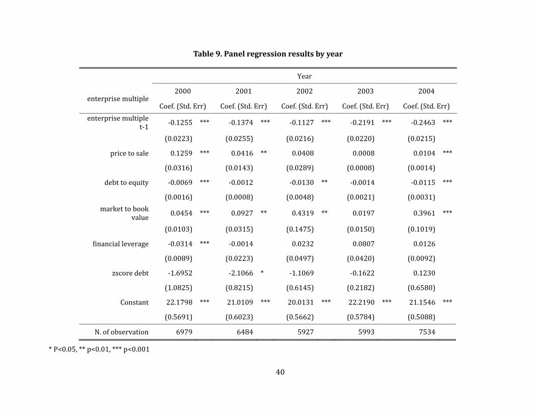
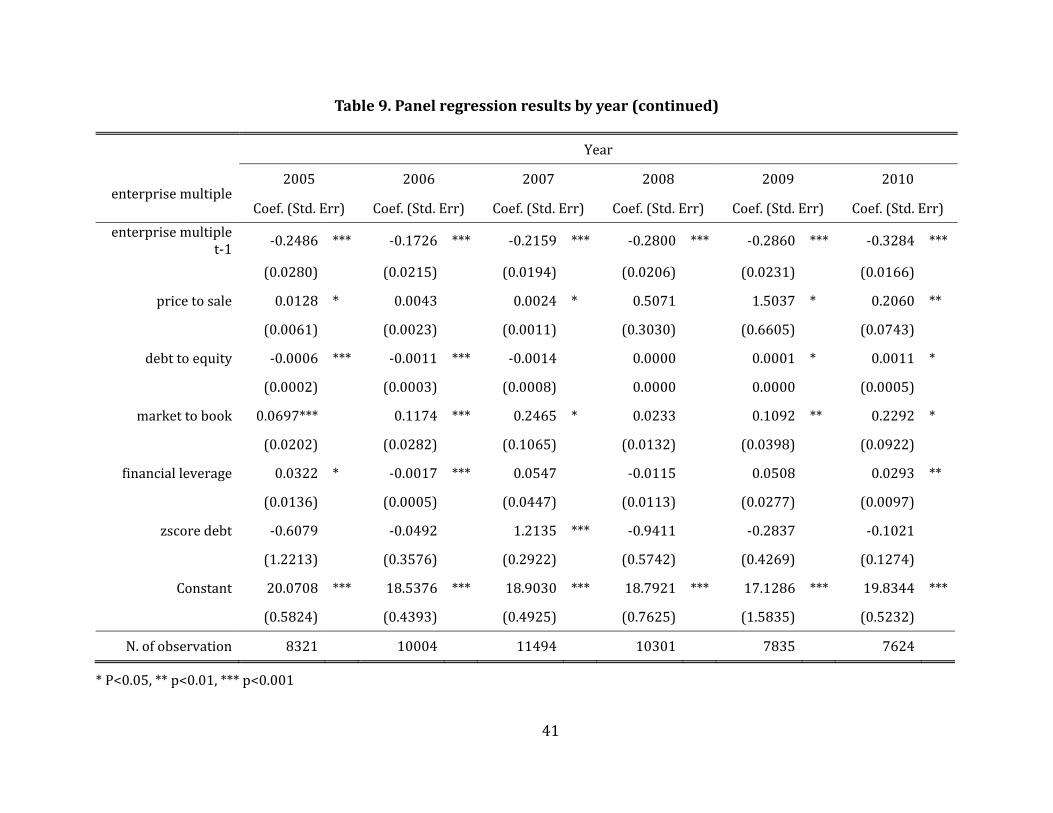
Next, we perform the Arellano and Bond dynamic panel regression for each year. Table 9
presents the regression results in each year of 2000 to 2010. The results show the general case
with lagged enterprise multiple and all five controls as before. In the year of 2000 and 2004-2007,
2TheWooldridge test for autocorrelation in the panel confirms a first order autocorrelation in enterprisemultipleforoveralldata:Wooldridgetestforautocorrelationinpaneldata;H0:nofirstorderautocorrelation;F(1,26963)=1533.254;Prob>F=0.0000.
16
we experienced business peaks in the market, during which the total number of M&A activities
increased rapidly. From the regression results in Table 9, almost all the financial fundamental
ratios (excluding financial leverage) command significant effects on firm value in the year of
2000 and 2004~2007. For example, an increase of one unit in market to book ratio can bring up
the enterprise multiple by 39% in the year of 2004, say from 1.00 to 1.39.
As often occurs in a peak-and-trough cycle, growth that takes place in a boom is rarely
maintained and backed up by actual company profits. In the year of 2001 to 2003, 2008 and 2009,
the dynamic panel model doesn’t identify such significant effect of the control variables on firm
values. The price to sale, debt to equity and market to book ratios are only significant at 5% level
occasionally at the year of 2001, 2002, 2009 and 2010; while none of them are significant in
2003 and 2008 at all.
From a perspective of year by year, the contemporaneous effect of price to sales, debt to
equity and market to book ratios on EV/EBITDA are more likely to be significant in peak years
in the 2000s and quantitative larger in magnitude than financial leverage. During trough years,
firms operate less efficiently and may even go bankrupt; under pressure of recession, firm value
is not highly sensitive to its own financial fundamentals, thus we can hardly estimate the
enterprise multiple only by financial ratios. On the other hand, the firm’s current value is always
much more sensitive to the lagged value ranging from -11% to -33%; this result is consistent for
firms in all company sectors and persistent across years.
4.2. Treatment Effects
We estimate several treatment effects econometric models below. First, we estimate regressions
with time dummy variables. We control for time effects on firm values in the period of seven
years using a set of time dummy variables:
∑ (3)
where i indexes the observation and dtit is the time dummy defined by relative year (dt):
17
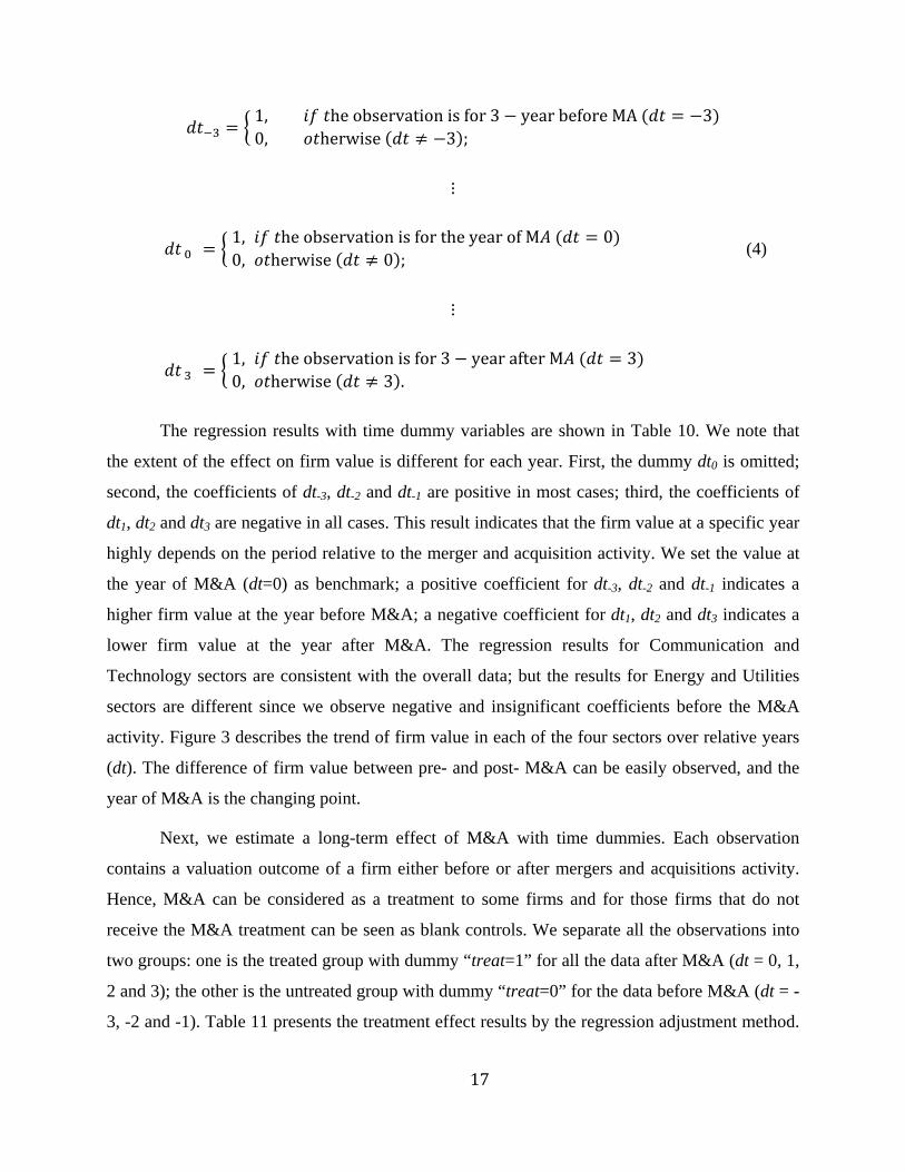
1, heobservationisfor3 yearbeforeMA 30, herwise 3 ;
⋮
1, heobservationisfortheyearofM 00, herwise 0 ;
(4)
⋮
1, heobservationisfor3 yearafterM 30, herwise 3 .
The regression results with time dummy variables are shown in Table 10. We note that
the extent of the effect on firm value is different for each year. First, the dummy dt0 is omitted;
second, the coefficients of dt-3, dt-2 and dt-1 are positive in most cases; third, the coefficients of
dt1, dt2 and dt3 are negative in all cases. This result indicates that the firm value at a specific year
highly depends on the period relative to the merger and acquisition activity. We set the value at
the year of M&A (dt=0) as benchmark; a positive coefficient for dt-3, dt-2 and dt-1 indicates a
higher firm value at the year before M&A; a negative coefficient for dt1, dt2 and dt3 indicates a
lower firm value at the year after M&A. The regression results for Communication and
Technology sectors are consistent with the overall data; but the results for Energy and Utilities
sectors are different since we observe negative and insignificant coefficients before the M&A
activity. Figure 3 describes the trend of firm value in each of the four sectors over relative years
(dt). The difference of firm value between pre- and post- M&A can be easily observed, and the
year of M&A is the changing point.
Next, we estimate a long-term effect of M&A with time dummies. Each observation
contains a valuation outcome of a firm either before or after mergers and acquisitions activity.
Hence, M&A can be considered as a treatment to some firms and for those firms that do not
receive the M&A treatment can be seen as blank controls. We separate all the observations into
two groups: one is the treated group with dummy “treat=1” for all the data after M&A (dt = 0, 1,
2 and 3); the other is the untreated group with dummy “treat=0” for the data before M&A (dt = -
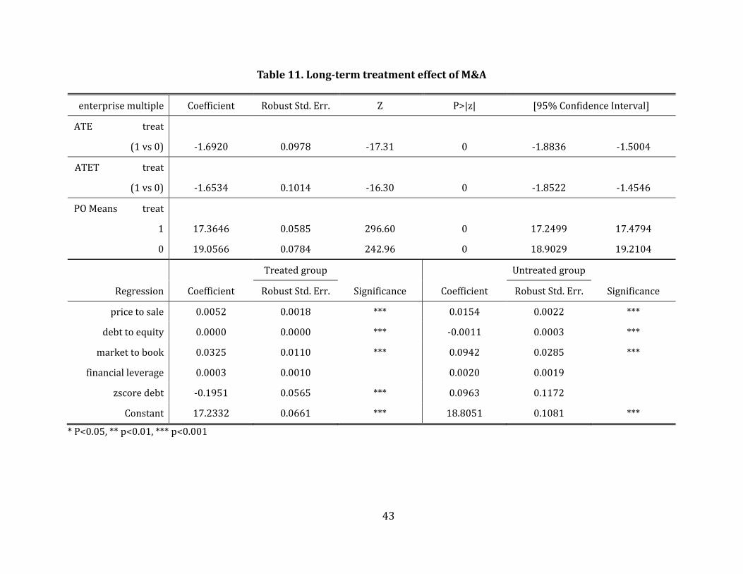
3, -2 and -1). Table 11 presents the treatment effect results by the regression adjustment method.
18
First we note that the potential outcome mean is 17.36 for the treated group and 19.05 for the
untreated group, thus the average treatment effect is -1.69. The potential outcome mean of
EV/EBITDA for firms after M&A is lower than that before the M&A deal, and this difference is
statistically significant. Moreover, from the regressions, the P/S, D/E and M/B ratios are highly
significant in both groups, a lower magnitude in the treated one; while ZD is significant after
M&A but not before, because an acquirer would have to take on the target’s entire debt which is
a huge impact on their accounting after M&A.
The results above indicate that EV/EBITDA varies from sector to sector. Higher firm
values are expected in high growth industries (like Technology) and lower multiples in industries
with slow growth (like Utilities). It's important to compare EV/EBITDA multiple within the
same industry in general. Thus, the average treatment effect of M&A on the separate sectors
should be also different. Table 12 summarizes the average treatment effect of M&A in each
sector separately. Those results are estimated by three different econometric methods: regression
adjustment, propensity score matching and nearest neighborhood matching. The ATEs are
always significant in Communication and Technology sectors, but insignificant in Energy and
Utilities sectors. As shown in Figure 4, the M&A activities in different sectors affect firm values
to different extents.
We proceed estimating the instantaneous effect of M&A from the treatment perspective.
Besides the discrepancy of firm values pre- and post- mergers and acquisitions activities, another
pattern emerges from Figure 4. There is an increase in the middle pomit on each line of
EV/EBITDA. The value gets stimulated at the time when M&A takes place. We design another
model to test this hypothesis. Again we separate all the observations into two groups but with
different assignments: one is the treated group with dummy “M&A=1” just for the data at the
year of M&A (dt = 0); the other is the untreated group with dummy “M&A=0” for all the rest of
data at the years with no M&A happening (dt = -3, -2, -1 and 1, 2, 3).
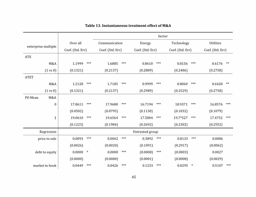
Table 13 presents the treatment effect results using the regression adjustment method.
First, we note that the potential outcome mean is 19.06 for treated group and 17.86 for untreated
group, thus the average treatment effect is +1.2. The potential outcome mean of EV/EBITDA for
firms being experiencing M&A is higher than those having no M&A activity during that year,
and this difference is significant. More importantly, this instantaneous effect of M&A activity on

19
EV/EBITDA is significant on all firms no matter which sector it belongs to. We also note that
the greatest increase of 1.6 in the enterprise multiple appears at Communication sector, followed
by an increase of 0.8 from Technology and Energy sectors, and a lowest increase 0.6 from the
Utilities sector. Therefore, a firm generally has higher EV/EBITDA ratio when M&A takes place.
Finally, we apply the difference-in-difference (DID) method to analyze the data in
partitions of two consecutive years. Taking the years of 2000 and 2001 as an example, the
experiment is designed as shown in Table 14a. In Table 14b we note that for 2000-2001, the
sample includes 10,192 observations, in which 5,849 of them are from the control group (no
M&A activity in both year of 2000 and 2001) and other 4,343 are from the treated group (no
M&A in year 2000 but M&A in year of 2001).
First, we estimate the DID without covariates. We estimate the regression of firm’s
EV/EBITDA with time dummy Year2001, state dummy M&A2001, and composite dummy
DiD2001 = Year2001 * M&A2001. This OLS regression analysis is equivalent to estimation
with only binary period and treatment variables. The results may be subject to biases, because
simple difference estimation proceeds under the assumption that the treatment and control groups
are the same in every respect apart from the treatment. However, we cannot guarantee that, in the
absence of treatment, the unobserved differences between treatment and control groups are the
same over time. Thus, we can specify some pre-treatment covariates of the model as optional
controls; and these variables are used to estimate the propensity score. We use the covariates P/S,
D/E, M/B, FL and ZD. Table 15a shows the results for 2000-2001 in both cases. In the case of
no covariates, the coefficient of DiD2001 is -1.99 with p-value 0.016. This result indicates that
the firm’s EV/EBITDA value after M&A is lower than those without M&A activities, and this
effect is statistically significant. The DID estimate with covariates (P/S, D/E, M/B, FL and ZD)
is -2.037, close to the results above, and also statistically significant. Hence, mergers and
acquisitions activities in the year of 2001 lower the firm’s EV/EBITDA.
Tables 15b-15i repeat the analysis above for all pairs of subsequent years up to 2008-
2009. The results for M&A in 2002, 2005, 2006 and 2007 shows negative effects on the firm
EV/EBITDA for both cases with and without covariates, but the estimates are not statistically
significant. In the other years of 2003, 2004 and 2009 the effect of M&A on value is positive but
not statistically significant. The key result is the 2007-2008 pair in Table 15h. It shows a highly
20
statistically significant positive effect of M&A on firms EV/EBITDA of the order of magnitude
of 2.409 without covariates and 1.726 with covariates. The importance of this result is that 2008
is the year of the U.S. financial crisis thus providing evidence that in a year of extreme financial
stress, M&A provided a source of counter balance in the sense of positive effects on firms
EV/EBITDA.
4.3 Discussion
First, from the two treatment experiments above, we find that the long-term effect of M&A
activity on firms’ EV/EBITDA is different from the instantaneous effect. The enterprise value
ratio multiple is defined as ratio of enterprise value to the earning. In general EV and EBITDA
increase over time, but the ratio may go up, down or even stay flat depending on the relative
changes. In the long-term treatment effect analysis, ATE on enterprise multiple is negative,
which means the ratio EV/EBITDA falls after M&A. While both the numerator and denominator
may rise, but the ratio falls, one possible explanation is that EBITDA in the denominator
increases faster than EV in the numerator. In other words, during the three years after M&A
activity, earnings grow farther than the corresponding enterprise value. This result is valid in
technology-related firms, but not in energy-related companies.
From the perspective of high-tech business, the motivation of mergers and acquisitions
are clear, to seek innovation in technology and acquire intellectual property. Acquirer firms
could apply the new technology immediately and become more productive resulting in the raise
of total revenue and profit in a short time period. Concurrently, firms are not required to largely
expand total assets and market capitalization. Thus, the increase of enterprise value could be less
than that of firm’s earnings during the three years after the M&A deal, which results in a fall of
EV/EBITDA. Also, a lower EV/EBITDA means the firm is more valuable. Therefore, M&A is
good for technology-intensive companies because of the enhancement in firms’ development.
However, Energy and Utilities firms show a different pattern. The main incentive for
M&A in those sectors should be tangible advantage. Firms get geographic expansion and occupy
more resources after a deal, especially in a cross-border deal. Firm’s earnings increase at the
same pace as enterprise value or even slower, thus the EV/EBITDA ratio fluctuates much less
during the post-merger three-year period. The payoff from M&A may take longer than three

21
years in resource-intensive firms. Therefore, the EV/EBITDA of Energy and Utilities sector does
not dramatically change during that period.
In the instantaneous treatment effect analysis, ATE on EV/EBITDA is positive, which
means the ratio of EV/EBITDA goes up at the time when mergers and acquisitions take place.
While both the numerator and denominator raise up so does the ratio, and we conjecture
instantaneously the EV in the numerator increases more than EBITDA in the denominator. In
other words, enterprise value grows faster than firm’s earning in the year of M&A. When a deal
is announced or completed, the acquirer expects greater gains from the combination or
reconstruction as well as shareholders expect a profitable outcome. The stock price becomes very
sensitive and responds fast, e.g. the first 7-day change or first 30-day change is much higher than
normal. Thus, enterprise value has an upward tick at the moment of the M&A. But firm’s
earnings cannot respond as quickly as the stock market, it responds in a much slower fashion.
Therefore, we observe stimulation on EV/EBITDA ratio just at the year of the M&A, and firm
value temporarily goes up. This instantaneous effect is significant, in general, on all four
company sectors.
Finally, the DID estimations for the sequence of two consecutive years shows a
significant negative effect of M&A activity on firm value in 2001 relative to 2000. However, it
shows a strong positive effect of M&A activity in 2008 relative to 2007. The other years are not
statistically significant. This is an important finding because relative to 2000, 2001 is a recession
year and relative to 2007, 2008 represents the impact of the financial crisis. We show that in the
universe of M&A activity, the financial crisis had a distinct positive impact on the value of firms
through M&A relative to the recession of 2001.
5. Conclusions
We provide extensive empirical evidence of mergers and acquisitions (M&A) effects on firm
value using a variety of econometric models and design. We use a large sample of 65,000 firms
from the sectors of Communications, Technology, Energy and Utilities. It includes worldwide
M&A deals during the years of 2000 to 2010.
22
We use an enterprise value multiple, the ratio of EV/EBITDA, as a measure of firm value,
and other financial fundamental ratios as controls, specifically price to sale ratio, debt to equity
ratio, market to book ratio and financial leverage. The small time and large cross-sectional
dimensions make the Arellano-Bond dynamic panel methodology appropriate. Our first result
shows consistent and robust evidence that market to book ratios provide a significant positive
effect on enterprise multiple across the universe of firms in all four company sectors. Price to
sale ratio has the similar effect but only significant in some cases. In the case of leverage, the
debt to equity ratio has a significant negative impact on EV/EBITDA in Energy and Utilities
sectors. A lower market-to-book ratio and a higher debt-to-equity ratio decrease the EV/EBITDA
ratio indicating an undervalued firm. However, financial leverage is not consistent in all cases.
From a perspective of time, our evidence on firm value shows that the contemporaneous
effect of price to sales, debt to equity and market to book ratios are significant and larger in
magnitude in peak years of the business cycle. However, we do not find a significant impact
from financial leverage for this set of firms. During trough years, those financial fundamental
ratios are not good predictors of firm value. In addition, the firm current values are sensitive to
lagged values indicating potential for over and under reaction of firm value.
The evidence from treatment effects shows that long-term and instantaneous effects on
the EV/EBITDA are much different. In the long-term, three years pre- and post- the deal, M&A
gives a net decrease in EV/EBITDA. This is because of a potential higher increase in firm’s
earnings relative to enterprise value in the longer horizon. The time effects are significant in
technology-intensive firms while not in resource-intensive firms. By contrast, the instantaneous
effect of M&A on firm value is more uniform in all four sectors. The firm value gets an
instantaneous increase at the time of the M&A deal, since the EV via the stock market moves
much faster in response to the M&A activity while the enhancement in firms’ earnings is slow
moving.
The difference-in-difference (DID) with propensity score matching estimations for the
sequence of two consecutive years shows a significant negative effect of M&A activity on firm
value in 2001 relative to 2000. However, it shows a strong positive effect of M&A activity in
2008 relative to 2007 and the other years are not statistically significant. We find this to be an
important result because relative to 2000, 2001 is a recession year and relative to 2007, 2008

23
represents the impact of the financial crisis. We show that in the universe of M&A activity, the
financial crisis had a distinct positive impact on the value of firms through M&A relative to the
recession of 2001.
We only included the firm-level M&A effects in this work. A fruitful avenue for future
research would be to expand a longer time period pre- and post- M&A, add market characteristic
information at each year, include the original countries of acquirer and target and specify cash or
stock financing method and horizontal or vertical deal structure, to better understand the trends
and other potential effects of mergers and acquisitions on firm values.
References
Abadie, A., Drukker, D., Herr, J.L. and Imbens, G.W. (2004), "Implementing matching estimators for average treatment effects in Stata", Stata Journal 4 (3):290-311.
Abadie, A. and Imbens, G.W. (2006), "Large Sample Properties of Matching Estimators for Average Treatment Effects", Econometrica 74 (1):235-267.
Abadie, A. and Imbens, G.W. (2011), "Bias-Corrected Matching Estimators for Average Treatment Effects", Journal of Business and Economic Statistics 29 (1).
Abadie, A. and Imbens, G.W. (2012), "Matching on the estimated propensity score", Harvard University and National Bureau of Economic Research Policy.
Abellán, D. (2004), Mergers and Acquisitions: a survey of motivations. Documento de trabajo 0401. Universidad Complutense de Madrid.
Agrawal, A. and Jaffe, J.F. (2000), "The post-merger performance puzzle", Advances in Mergers & Acquisitions 1 (Emerald Group Publishing Limited):7-41.
Auerbach, A.J. and Reishus, D. (1987), "The Impact of Taxation on Mergers and Acquisitions" Mergers and Acquisitions: University of Chicago Press, 69-86.
Baker, G.P., Jensen, M.C. and Murphy, K.J. (1988), "Compensation and Incentives: Practice vs. Theory", The Journal of Finance 43 (3):593-616.
Barney, J. (1991), "Firm Resources and Sustained Competitive Advantage", Journal of Management 17 (1):99-120.
Berkovitch, E. and Narayanan, M.P. (1993), "Motives for Takeovers: An Empirical Investigation", Journal of Financial and Quantitative Analysis 28 (3):347-362.
Bradley, M., Desai, A. and Kim, E.H. (1988), "Synergistic gains from corporate acquisitions and their division between the stockholders of target and acquiring firms", Journal of Financial Economics 21 (1):3-40.
Cameron, A.C. and Trivedi, P.K. (2005), "Microeconometrics: Methods and Applications", New York: Cambridge University Press.
Cassiman, B. and Colombo, M.G. (2006), "Mergers and Acquisitions: The Innovation Impact", Chapter 3, Cheltenham, UK: Edward Elgar Publishing, Inc.
Caves, R.E. (1989), "Mergers, takeovers, and economic efficiency: Foresight vs. hindsight", International Journal of Industrial Organization 7 (1):151-174.
Chapman, K. (2003), "Cross‐border mergers/acquisitions: a review and research agenda", Journal of Economic Geography 3 (3):309-334.

Chen, C. and Findlay, C. (2003), "A Review of Cross-border Mergers and Acquisitions in APEC", Asian-Pacific Economic Literature 17 (2):14-38.
Conyon, M.J. and Gregg, P. (1994), "Pay at the Top: A Study of the Sensitivity of Top Director Remuneration to Company Specific Shocks", National Institute Economic Review 149 (1):83-92.
Deyoung, R., Evanoff, D. and Molyneux, P. (2009), "Mergers and Acquisitions of Financial Institutions: A Review of the Post-2000 Literature", Journal of Financial Services Research 36 (2-3):87-110.
Erel, I., Jang, Y. and Weisbach, M.S. (2012), "Financing-Motivated Acquisitions", National Bureau of Economic Research Working Paper Series No. 17867.
Firth, M. (1991), "Corporate takeovers, stockholder returns and executive rewards", Managerial and Decision Economics 12 (6):421-428.
Frohlich, C. and Kavan, C.B. (2000), "An Examination of Bank Merger Activity: A Strategic Framework Content Analysis", Academy of Accounting and Financial Studies Proceedings.
Hall, B.H. (1990), "The Impact of Corporate Restructuring on Industrial Research and Development", Brookings Papers on Ecnomic Activity (Microeconomics):85-124.
Hitt, M.A., Hoskisson, R.E., Ireland, R.D. and Harrison, J.S. (1991), "Effects Of Acquisitions on R&D Inputs and Outputs", Academy of Management Journal 34 (3):693-706.
Hitt, M.A., Hoskisson, R.E., Johnson, R.A. and Moesel, D.D. (1996), "The Market for Corporate Control and Firm Innovation", The Academy of Management Journal 39 (5):1084-1119.
Jensen, M.C. and Ruback, R.S. (1983), "The market for corporate control: The scientific evidence", Journal of Financial Economics 11 (1–4):5-50.
Jongwanich, J., Brooks, D.H. and Kohpaiboon, A. (2013), "Cross-border Mergers and Acquisitions and Financial Development: Evidence from Emerging Asia", Asian Economic Journal 27 (3):265-284.
King, D.R., Dalton, D.R., Daily, C.M. and Covin, J.G. (2004), "Meta-analyses of post-acquisition performance: indications of unidentified moderators", Strategic Management Journal 25 (2):187-200.
King, D.R., Slotegraaf, R.J. and Kesner, I. (2008), "Performance Implications of Firm Resource Interactions in the Acquisition of R&D-Intensive Firms", Organization Science 19 (2):327-340.
Kumar, R. (2009), "Post-merger corporate performance: an Indian perspective", Management Research News 32 (2):145 - 157.
Kumar, V. and Singh, S.R. (1994), "Corporate rehabilitation and B.I.F.R.", New Delhi: Shipra Publications.
Kwoka, J.E., Jr. (2002), "Review of: Mergers and productivity", Journal of Economic Literature 40 (2):540-541.
Lane, P.W. and Nelder, J.A. (1982), "Analysis of covariance and standardization as instances of prediction", Biometrics 38 (3):613-621.
Lichtenberg, F.R. (1992), "Corporate Takeovers and Productivity", Cambridge, MA: MIT Press.
Manne, H.G. (1965), "Mergers and the Market for Corporate Control", Journal of Political Economy 73 (2):110-120.
Mantravadi, D.P. and Reddy, A.V. (2007), "Relative Size in Mergers and Operating Performance: Indian Experience", Economic and Political Weekly:September 29, 2007.
Mantravadi, D.P. and Reddy, A.V. (2008), "Post-Merger Performance of Acquiring Firms from Different Industries in India", International Research Journal of Finance and Economics 22.
Menapara, M.R. and Pithadia, V. (2012), "Review of Literature of Merger and Acquisition", GLOBAL RESEARCH ANALYSIS 1 (4):50-51.
Mueller, D.C. (1980), "The Determinants and Effects of Mergers: An International Comparison", Cambridge, MA: Oelgeschlager, Gunn & Hain.
Pawaskar, V. (2001), "Effect of Mergers on Corporate Performance in India", Vikalpa 26 (1):19-32.
Ranft, A.L. and Lord, M.D. (2002), "Acquiring New Technologies and Capabilities: A Grounded Model of Acquisition Implementation", Organization Science 13 (4):420-441.
Ravenscraft , D.J. and Scherer, F.M. (1987), "Mergers, sell-offs, and economic efficiency", Washington, DC: Brookings Institution.
Röller, L.-H., Stennek, J. and Verboven, F. (2000), "Efficiency gains from mergers", European Economy 5.
Rosenbaum, P.R. and Rubin, D.B. (1983), "The central role of the propensity score in observational studies for causal effects", Biometrika 70 (1):41-55.
Rubin, D.B. (1973), "Matching to Remove Bias in Observational Studies", Biometrics 29 (1):159-183.
Rubin, D.B. (1977), "Assignment to Treatment Group on the Basis of a Covariate", Journal of Educational and Behavioral Statistics 2 (1):1-26.
Sanker, R. and Rao, K.V. (1998), "Financial Management", 12-19.
Saple, V. (2000), "Diversification, Mergers and their Effect on Firm Performance: A Study of the Indian Corporate Sector", IGIDR, Mumbai: Ph.D. thesis.
Schulz, N. (2007), "Review of the literature on the impact of mergers on innovation".
Sevilir, M. and Tian, X. (2012), "Acquiring Innovation", AFA 2012 Chicago Meetings Paper.
Straub, T. (2007), "Reasons for frequent failure in Mergers and Acquisitions: A comprehensive analysis" Gabler Edition Wissenschaft, Wiesbaden: Deutscher Universitäts-Verlag (DUV).
SzüCs, F. (2013), "M&A and R&D: Asymmetric Effects on Acquirers and Targets?".
Vanitha, S. and Selvam, M. (2007), "Financial Performance of Indian Manufacturing Companies During Pre and Post Merger", International Research Journal of Finance and Economics 12:7-35.
Vittinghoff, E., Glidden, D.V., Shiboski, S.C. and Mcculloch, C.E. (2012), "Regression Methods in Biostatistics: Linear, Logistic, Survival, and Repeated Measures Models", 2nd ed, New York: Springer.
Wooldridge, J.M. (2010), "Econometric Analysis of Cross Section and Panel Data", 2nd ed, Cambridge, MA: MIT Press.
28
Table1.Top‐valueM&Aglobaldealsin21stcentury
Rank Year Acquirer Target Transactionvalue(inbillonUSD)
2000's 1 2000 AOLInc.(AmericaOnline) TimeWarner 164.75
2 2000 GlaxoWellcomePlc. SmithKlineBeechamPlc. 75.96
3 2004 RoyalDutchPetroleumCompany ShellTransport&TradingCo. 74.56
4 2006 AT&TInc BellSouthCorporation 72.67
5 2001 ComcastCorporation AT&TBroadband 72.04
6 2009 PfizerInc. Wyeth 68
7 2000 NortelNetworksCorporation 59.97
8 2002 PfizerInc. PharmaciaCorporation 59.52
9 2004 JPMorganChase&Co BankOneCorporation 58.76
10 2008 InBeyInc. Anheuser‐BuschCompanies,Inc. 52
2010‐ 1 2014 ComcastCorporation TimeWarnerCable 45.2
2 2012 DeutscheTelekom MetroPCS 29
3 2013 BerkshireHathaway H.J.HeinzCompany 28
4 2013 Softbank SprintCorporation 21.6
5 2014 Facebook WhatsApp 19
6 2011 Google MotorolaMobility 9.8
7 2011 BerkshireHathaway Lubrizol 9.22
8 2011 MicrosoftCorporation Skype 8.5

29
Table2.Companysectorsclassification
CompanySectors COMMUNICATIONS ENERGY TECHNOLOGY UTILITIES
Sub‐sectors
Advertising Coal Computers Electric
Internet Energy‐Alternate
SourcesOffice/BusinessEquip
Gas
Media Oil&Gas Semiconductors WaterTelecommunications Oil&GasServices Software
Pipelines

30
Table3.M&Adealvolumebysectorandyear
YearSector
TotalCommunication Technology Energy Utilities
2000 4583 2421 1046 538 8588
2001 3109 1718 973 471 6271
2002 2115 1320 780 417 4632
2003 1809 1312 887 345 4353
2004 2333 1437 1051 406 5227
2005 2588 1588 1203 404 5783
2006 2928 1821 1345 490 6584
2007 3008 1913 1656 548 7125
2008 2535 1718 1489 632 6374
2009 1907 1372 1264 496 5039
2010 2160 1525 1392 468 5545
Sum 29075 18145 13086 5215 65521
31
Table4a.Datadistributioninsectors
Group(sector)
Sector 1 2 3 4 Total
Communication 67,608 67,608
Energy 30,088 30,088
Technology 46,419 46,419
Utilities 21,545 21,545
Total 67,608 30,088 46,419 21,545 165,660
32
Table4b.Datadistributioninyears
Dt Frequency Percent
‐3 18,573 11.21
‐2 21,123 12.75
‐1 23,865 14.41
0 26,081 15.74
1 26,184 15.81
2 25,690 15.51
3 24,144 14.57
Total 165,660 100
Note:DtreferstothetimingoftheM&Adeal,where0istheyearthedealtakesplace
33
Table5a.Descriptivestatisticsoforiginaldata
Variable Observation MeanStandardDeviation Minimum Maximum
enterprisemultiple
(EV/EBITDA)172736 45.48 809.79 0 1.05E+05
enterprisevalue(EV)
277619 2.91E+05 4.13E+06 ‐1.00E+06 2.34E+08
Earnings 218129 2.52E+04 5.00E+05 ‐3.59E+06 2.88E+07
marketcapitalization 300847 2.24E+05 3.71E+06 0 2.24E+08
totaldebt 293223 5.44E+04 6.24E+05 ‐225 5.95E+07
pricetosale 284253 49.80 2956.86 0 5.02E+05
debttoequity 280310 289.57 3.18E+04 ‐611.57 7.57E+06
markettobookvalue 279568 14.65 2.36E+03 ‐8.67E+04 5.88E+05
financialleverage
279986 3.00 156.42 ‐1.02E+04 3.12E+04
zscoredebt 293223 ‐9.58E‐19 1 ‐0.09 95.20
34
Table5b.Descriptivestatisticsoftrimmeddata
Variable Observation MeanStandardDeviation Minimum Maximum
enterprisemultiple
(EV/EBITDA)
165660 18.22 18.49 1.00 149.71
enterprisevalue(EV) 165572 3.58E+05 5.20E+06 ‐1108.40 2.34E+08
Earning 153959 3.43E+04 5.91E+05 ‐3.59E+06 2.88E+07
marketcapitalization 164645 3.14E+05 4.94E+06 0.0012 2.24E+08
totaldebt 158680 5.10E+04 6.17E+05 ‐225 2.69E+07
pricetosale 164725 4.13 63.31 0 9606.70
debttoequity 156381 114.5116 2942.81 0 4.47E+05
markettobookvalue
164937 3.43 157.40 ‐1171.59 4.48E+04
financialleverage
156834 2.69 48.24 ‐10215.23 1635.59
zscoredebt 158680 ‐7.26E‐18 1 ‐0.08 43.54
35
Table6.Pairwisecorrelations
enterprisemultiple
(EV/EBITDA)
enterprisevalue
earning marketcapitalization
totaldebt pricetosale
debttoequity
markettobook
financialleverage
zscoredebt
enterprisemultiple
(EV/EBITDA)
1
enterprisevalue
‐0.0147* 1
0.0000
earning‐0.0272* 0.9033* 1
0.0000 0.0000
marketcapitalization
‐0.0151* 0.9887* 0.9138* 1
0.0000 0.0000 0.0000
totaldebt‐0.0059 0.6662* 0.6494* 0.5977* 1
0.0196 0.0000 0.0000 0.0000
pricetosale0.0241* ‐0.0022 ‐0.0021 ‐0.0020 ‐0.0032 1
0.0000 0.3816 0.4102 0.4283 0.1972
debttoequity0.0035 ‐0.0013 ‐0.0015 ‐0.0015 ‐0.0009 ‐0.0006 1
0.1671 0.6172 0.5586 0.5471 0.7341 0.8082
markettobookvalue
0.0031 ‐0.0001 ‐0.0002 0.0000 ‐0.0006 0.0002 0.0023 1
0.2060 0.9800 0.9429 0.9902 0.8028 0.9347 0.3562
financialleverage
0.0045 ‐0.0002 ‐0.0007 ‐0.0005 ‐0.0001 ‐0.0007 0.0052 0.0233* 1
0.0780 0.9236 0.7780 0.8318 0.9624 0.7945 0.0395 0.0000
zscoredebt‐0.0059 0.6662* 0.6494* 0.5977* 1.0000* ‐0.0032 ‐0.0009 ‐0.0006 ‐0.0001 1
0.0196 0.0000 0.0000 0.0000 0.0000 0.1972 0.7341 0.8028 0.9624
*p<0.01
36
Figure1.M&Adealvolumebysectorandyear
0
2,000
4,000
6,000
8,000
10,000
MergersandAcquisitionsVolume
Year
Total Communication Energy Technology Utilities
37
Figure2.DistributionofEV/EBITDA
0
.05
.1.1
5.2
.25
0.0
5.1
.15
.2.2
5
mean1sd 1sd 2sd 3sd 4sd 5sd 6sd 7sd mean1sd 1sd 2sd 3sd 4sd 5sd 6sd 7sd
0 50 100 150 0 50 100 150
Communication Energy
Technology Utilities
Frac
tion
EV/EBITDAGraphs by sector
0.0
5.1
.15
.2Fr
actio
n
mean1sd 1sd 2sd 3sd 4sd 5sd 6sd 7sd
0 50 100 150EV/EBITDA
38
Table7.Fixed‐effectpanelregressionresultsoverallandbysector
Sector
enterprisemultipleOverall Communication Energy Technology Utilities
Coef.(Std.Err) Coef.(Std.Err) Coef.(Std.Err) Coef.(Std.Err) Coef.(Std.Err)
pricetosale 0.0079 ** 0.0059 ** 0.1929 ** 1.2714 *** 0.0404
(0.0027) (0.0022) (0.0694) (0.1806) (0.0292)
debttoequity 0.0000 0.0000 ‐0.0012 *** 0.0008 ‐0.0127 ***
0.0000 0.0000 (0.0002) (0.0006) (0.0023)
markettobook 0.0392 *** 0.0333 *** 0.1702 *** 0.0260 1.1303 ***
(0.0086) (0.0085) (0.0236) (0.0164) (0.1575)
financialleverage 0.0020 0.0047 *** ‐0.0029 *** 0.0183 *** 0.1035 *
(0.0012) (0.0006) (0.0005) (0.0055) (0.0453)
zscoredebt 0.1316 ‐0.4205 ‐0.0363 0.5856 ** 0.8925 **
(0.1301) (0.3490) (0.1079) (0.1870) (0.2954)
Constant 17.8932 *** 18.0859 *** 16.1007 *** 15.9760 *** 15.5759 ***
(0.0305) (0.0353) (0.1667) (0.4188) (0.4032)
R‐squared 0.0023 0.0027 0.0140 0.0469 0.0182
N.ofobservation 153256 61972 28101 42964 20219
*P<0.05,**p<0.01,***p<0.001
39
Table8.Dynamicpanelregressionresultsoverallandbysector
Sector
enterprisemultipleOverall Communication Energy Technology Utilities
Coef.(Std.Err) Coef.(Std.Err) Coef.(Std.Err) Coef.(Std.Err) Coef.(Std.Err)
enterprisemultiplet‐1 ‐0.2297 *** ‐0.1302 *** ‐0.3221 *** ‐0.2287 *** ‐0.3771 ***
(0.0064) (0.0110) (0.0134) (0.0110) (0.0158)
pricetosale 0.0053 0.0029 0.3438 ** 1.8373 *** 0.0268 *
(0.0034) (0.0020) (0.1214) (0.2832) (0.0121)
debttoequity 0.0000 0.0000 ‐0.0008 *** ‐0.0005 ‐0.0183 ***
0.0000 0.0000 (0.0002) (0.0007) (0.0040)
markettobook 0.0269 *** 0.0293 ** 0.1133 *** 0.0203 1.3128 ***
(0.0070) (0.0095) (0.0323) (0.0107) (0.1837)
financialleverage 0.0008 0.0177 ‐0.0017 *** ‐0.0282 0.2384 *
(0.0017) (0.0131) (0.0004) (0.0445) (0.1090)
zscoredebt ‐0.6316 ** ‐1.1244 *** ‐0.5027 0.5881 0.9942 ***
(0.2412) (0.2286) (0.4578) (0.3781) (0.1805)
Constant 20.7979 *** 18.8044 *** 20.2336 *** 18.1071 *** 21.5336 ***
(0.1502) (0.2543) (0.4057) (0.6924) (0.4405)
N.ofobservation 88496 35628 16007 23935 12926
*P<0.05,**p<0.01,***p<0.001
40
Table9.Panelregressionresultsbyyear
Year
enterprisemultiple2000 2001 2002 2003 2004
Coef.(Std.Err) Coef.(Std.Err) Coef.(Std.Err) Coef.(Std.Err) Coef.(Std.Err)
enterprisemultiplet‐1 ‐0.1255 *** ‐0.1374 *** ‐0.1127 *** ‐0.2191 *** ‐0.2463 ***
(0.0223) (0.0255) (0.0216) (0.0220) (0.0215)
pricetosale 0.1259 *** 0.0416 ** 0.0408 0.0008 0.0104 ***
(0.0316) (0.0143) (0.0289) (0.0008) (0.0014)
debttoequity ‐0.0069 *** ‐0.0012 ‐0.0130 ** ‐0.0014 ‐0.0115 ***
(0.0016) (0.0008) (0.0048) (0.0021) (0.0031)
markettobookvalue 0.0454 *** 0.0927 ** 0.4319 ** 0.0197 0.3961 ***
(0.0103) (0.0315) (0.1475) (0.0150) (0.1019)
financialleverage ‐0.0314 *** ‐0.0014 0.0232 0.0807 0.0126
(0.0089) (0.0223) (0.0497) (0.0420) (0.0092)
zscoredebt ‐1.6952 ‐2.1066 * ‐1.1069 ‐0.1622 0.1230
(1.0825) (0.8215) (0.6145) (0.2182) (0.6580)
Constant 22.1798 *** 21.0109 *** 20.0131 *** 22.2190 *** 21.1546 ***
(0.5691) (0.6023) (0.5662) (0.5784) (0.5088)
N.ofobservation 6979 6484 5927 5993 7534
*P<0.05,**p<0.01,***p<0.001
41
Table9.Panelregressionresultsbyyear(continued)
Year
enterprisemultiple2005 2006 2007 2008 2009 2010
Coef.(Std.Err) Coef.(Std.Err) Coef.(Std.Err) Coef.(Std.Err) Coef.(Std.Err) Coef.(Std.Err)
enterprisemultiplet‐1 ‐0.2486 *** ‐0.1726 *** ‐0.2159 *** ‐0.2800 *** ‐0.2860 *** ‐0.3284 ***
(0.0280) (0.0215) (0.0194) (0.0206) (0.0231) (0.0166)
pricetosale 0.0128 * 0.0043 0.0024 * 0.5071 1.5037 * 0.2060 **
(0.0061) (0.0023) (0.0011) (0.3030) (0.6605) (0.0743)
debttoequity ‐0.0006 *** ‐0.0011 *** ‐0.0014 0.0000 0.0001 * 0.0011 *
(0.0002) (0.0003) (0.0008) 0.0000 0.0000 (0.0005)
markettobook 0.0697*** 0.1174 *** 0.2465 * 0.0233 0.1092 ** 0.2292 *
(0.0202) (0.0282) (0.1065) (0.0132) (0.0398) (0.0922)
financialleverage 0.0322 * ‐0.0017 *** 0.0547 ‐0.0115 0.0508 0.0293 **
(0.0136) (0.0005) (0.0447) (0.0113) (0.0277) (0.0097)
zscoredebt ‐0.6079 ‐0.0492 1.2135 *** ‐0.9411 ‐0.2837 ‐0.1021
(1.2213) (0.3576) (0.2922) (0.5742) (0.4269) (0.1274)
Constant 20.0708 *** 18.5376 *** 18.9030 *** 18.7921 *** 17.1286 *** 19.8344 ***
(0.5824) (0.4393) (0.4925) (0.7625) (1.5835) (0.5232)
N.ofobservation 8321 10004 11494 10301 7835 7624
*P<0.05,**p<0.01,***p<0.001

42
Table10.Regressionresultswithtimedummyvariables
Sector
enterprisemultipleOverall Communication Energy Technology Utilities
Coefficient Coefficient Coefficient Coefficient Coefficient
pricetosale 0.0075 ** 0.0055 ** 0.1911 ** 1.1946 *** 0.0407
debttoequity 0.0000 0.0000 ‐0.0011 *** 0.0015 ** ‐0.0123 ***
markettobook 0.0343 *** 0.0265 *** 0.1665 *** 0.0191 1.1131 ***
financialleverage 0.0022 0.0048 *** ‐0.0028 *** 0.0178 *** 0.1031 *
zscoredebt 0.3704 ** 0.0594 0.0191 0.7482 *** 0.8881 **
dt‐3 1.3387 *** 1.8517 *** 0.5813 1.7828 *** ‐1.0803 ***
dt‐2 0.6347 *** 1.0444 *** 0.0558 0.6496 * ‐0.5282
dt‐1 0.7918 *** 1.4685 *** ‐0.1248 0.2642 0.0635
dt1 ‐1.6421 *** ‐2.4170 *** ‐1.0938 *** ‐1.0953 *** ‐0.1281
dt2 ‐2.8018 *** ‐3.7622 *** ‐1.4333 *** ‐2.4959 *** ‐0.9884 **
dt3 ‐3.3057 *** ‐4.7374 *** ‐1.4874 *** ‐2.6108 *** ‐1.0557 **
Constant 18.6876 *** 19.1775 *** 16.6380 *** 16.7320 *** 16.0693 ***
R‐squared 0.0173 0.0339 0.0171 0.0561 0.0202
N.ofobservation 153256 61972 28101 42964 20219
*P<0.05,**p<0.01,***p<0.001Negativevalueofdtcoefficientismarkedinred.
43
Table11.Long‐termtreatmenteffectofM&A
enterprisemultiple Coefficient RobustStd.Err. Z P>|z| [95%ConfidenceInterval]
ATEtreat
(1vs0) ‐1.6920 0.0978 ‐17.31 0 ‐1.8836 ‐1.5004
ATETtreat
(1vs0) ‐1.6534 0.1014 ‐16.30 0 ‐1.8522 ‐1.4546
POMeanstreat
1 17.3646 0.0585 296.60 0 17.2499 17.4794
0 19.0566 0.0784 242.96 0 18.9029 19.2104
Treatedgroup Untreatedgroup
Regression Coefficient RobustStd.Err. Significance Coefficient RobustStd.Err. Significance
pricetosale 0.0052 0.0018 *** 0.0154 0.0022 ***
debttoequity 0.0000 0.0000 *** ‐0.0011 0.0003 ***
markettobook 0.0325 0.0110 *** 0.0942 0.0285 ***
financialleverage 0.0003 0.0010 0.0020 0.0019
zscoredebt ‐0.1951 0.0565 *** 0.0963 0.1172
Constant 17.2332 0.0661 *** 18.8051 0.1081 ***
*P<0.05,**p<0.01,***p<0.001

44
Table12.Long‐termtreatmenteffectofM&Abysector
ATE Overall Communication Technology Energy Utility
Treatmenteffects Coef.(Std.Err) Coef.(Std.Err) Coef.(Std.Err) Coef.(Std.Err) Coef.(Std.Err)
regressionadjustment ‐1.6920 *** ‐2.4118 *** ‐1.6015 *** ‐0.2232 ‐0.0887
(0.0978) (0.1583) (0.2145) (0.2112) (0.2036)
propensityscorematching N/A N/A ‐0.9542 *** 0.1417 ‐0.0555
(0.2153) (0.1795) (0.1943)
nearestneighborhoodmatching ‐0.2071 *** ‐0.4720 *** ‐0.5461 ** 0.1397 0.2377
(0.0753) (0.1243) (0.2003) (0.1695) (0.1447)
*P<0.05,**p<0.01,***p<0.001
45
Table13.InstantaneoustreatmenteffectofM&A
Sector
enterprisemultipleOverall Communication Energy Technology Utilities
Coef.(Std.Err) Coef.(Std.Err) Coef.(Std.Err) Coef.(Std.Err) Coef.(Std.Err)
ATE
M&A 1.1999 *** 1.6885 *** 0.8610 *** 0.8156 *** 0.6176 **
(1vs0) (0.1321) (0.2137) (0.2889) (0.2486) (0.2758)
ATET
M&A 1.2128 *** 1.7185 *** 0.9999 *** 0.8060 *** 0.6428 **
(1vs0) (0.1321) (0.2137) (0.2989) (0.2529) (0.2758)
POMeanM&A
0 17.8611 *** 17.9680 *** 16.7194 *** 18.9371 *** 16.8576 ***
(0.0502) (0.0795) (0.1130) (0.1032) (0.1079)
1 19.0610 *** 19.6564 *** 17.5804 *** 19.7*527 *** 17.4752 ***
(0.1223) (0.1984) (0.2692) (0.2302) (0.2552)
Regression Untreatedgroup
pricetosale 0.0093 *** 0.0062 *** 0.3892 *** 0.8133 *** 0.0086
(0.0026) (0.0020) (0.1091) (0.2917) (0.0062)
debttoequity 0.0000 * 0.0000 *** (0.0008) *** (0.0003) 0.0027
(0.0000) (0.0000) (0.0001) (0.0008) (0.0029)
markettobook 0.0449 *** 0.0426 *** 0.1233 *** 0.0295 * 0.5107 ***

46
Table13‐cont.
(0.0109) (0.0121) (0.0171) (0.0168) (0.0930)
financialleverage 0.0012 0.0040 *** (0.0019) *** 0.0105 ** (0.5574) ***
(0.0010) (0.0008) (0.0004) (0.0053) (0.1643)
zscoredebt (0.0781) (0.3943) *** (0.9768) *** (0.9071) *** 0.9283 ***
(0.0621) (0.0273) (0.1071) (0.2199) (0.1285)
Constant 17.6706 *** 17.7654 *** 15.5676 *** 16.8710 *** 17.5986 ***
(0.0607) (0.0897) (0.2559) (0.6614) (0.3623)
Regression Treatedgroup
pricetosale 0.0026 0.0000 1.3035 *** 2.2073 *** 0.0040
(0.0018) (0.0015) (0.2248) (0.1915) (0.0079)
debttoequity (0.0014) *** (0.0010) *** (0.0006) (0.0010) 0.0142 ***
(0.0004) (0.0004) (0.0004) (0.0021) (0.0046)
markettobook 0.1559 *** 0.0923 *** 0.0857 0.3310 *** 1.0775 **
(0.0433) (0.0355) (0.0619) (0.1029) (0.5064)
financialleverage 0.0043 0.0053 0.0411 ** 0.0646 (1.1535) ***
(0.0040) (0.0041) (0.0196) (0.0643) (0.1720)
zscoredebt (0.1871) (0.5552) *** (0.9338) ** 0.9644 ** 1.1579 ***
(0.1397) (0.0475) (0.4219) (0.4722) (0.4288)
Constant 18.6959 *** 19.4929 *** 14.2510 *** 13.3477 *** 17.9251 ***
(0.1561) (0.2102) (0.5411) (0.4514) (0.9532)
*P<0.05,**p<0.01,***p<0.001
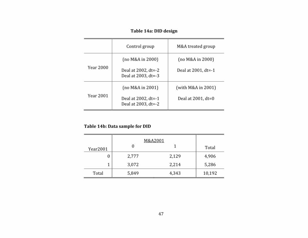
47
Table14a:DIDdesign
Controlgroup M&Atreatedgroup
Year2000
(noM&Ain2000)
Dealat2002,dt=‐2Dealat2003,dt=‐3
(noM&Ain2000)
Dealat2001,dt=‐1
Year2001
(noM&Ain2001)
Dealat2002,dt=‐1Dealat2003,dt=‐2
(withM&Ain2001)
Dealat2001,dt=0
Table14b:DatasampleforDID
M&A2001
Year20010 1 Total
0 2,777 2,129 4,906
1 3,072 2,214 5,286
Total 5,849 4,343 10,192
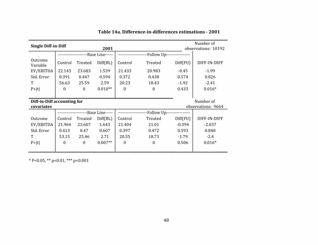
48
Table14a.Difference‐in‐differencesestimations‐2001
SingleDiff‐in‐Diff 2001 Numberof
observations:10192 ‐‐‐‐‐‐‐‐‐‐‐‐‐‐‐‐‐‐‐‐BaseLine‐‐‐‐‐ ‐‐‐‐‐‐‐‐‐‐‐‐‐‐‐‐‐‐‐‐FollowUp‐‐‐‐‐‐‐‐‐‐‐‐‐‐‐‐OutcomeVariable
Control Treated Diff(BL) Control Treated Diff(FU) DIFF‐IN‐DIFF
EV/EBITDA 22.143 23.683 1.539 21.433 20.983 ‐0.45 ‐1.99Std.Error 0.391 0.447 0.594 0.372 0.438 0.574 0.826T 56.63 25.59 2.59 20.23 18.43 ‐1.92 ‐2.41P>|t| 0 0 0.010** 0 0 0.433 0.016* Diff‐in‐Diffaccountingforcovariates Numberof
observations:9664 ‐‐‐‐‐‐‐‐‐‐‐‐‐‐‐‐‐‐‐‐BaseLine‐‐‐‐‐ ‐‐‐‐‐‐‐‐‐‐‐‐‐‐‐‐‐‐‐‐FollowUp‐‐‐‐‐‐‐‐‐‐‐‐‐‐‐‐ Outcome Control Treated Diff(BL) Control Treated Diff(FU) DIFF‐IN‐DIFFEV/EBITDA 21.964 23.607 1.643 21.404 21.01 ‐0.394 ‐2.037Std.Error 0.413 0.47 0.607 0.397 0.472 0.593 0.848T 53.15 25.46 2.71 20.55 18.73 ‐1.79 ‐2.4P>|t| 0 0 0.007** 0 0 0.506 0.016*
*P<0.05,**p<0.01,***p<0.001
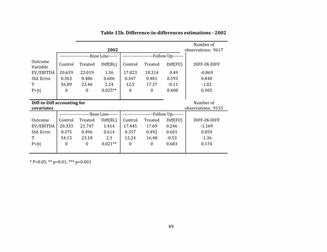
49
Table15b.Difference‐in‐differencesestimations‐2002
2002 Numberof
observations:9617 ‐‐‐‐‐‐‐‐‐‐‐‐‐‐‐‐‐‐‐‐BaseLine‐‐‐‐‐‐ ‐‐‐‐‐‐‐‐‐‐‐‐‐‐‐‐‐‐‐‐FollowUp‐‐‐‐‐‐‐OutcomeVariable
Control Treated Diff(BL) Control Treated Diff(FU) DIFF‐IN‐DIFF
EV/EBITDA 20.659 22.019 1.36 17.823 18.314 0.49 ‐0.869Std.Error 0.363 0.486 0.606 0.347 0.481 0.593 0.848T 56.89 23.46 2.24 12.5 17.37 ‐0.11 ‐1.02P>|t| 0 0 0.025** 0 0 0.408 0.305 Diff‐in‐Diffaccountingforcovariates Numberof
observations:9153 ‐‐‐‐‐‐‐‐‐‐‐‐‐‐‐‐‐‐‐‐BaseLine‐‐‐‐‐‐ ‐‐‐‐‐‐‐‐‐‐‐‐‐‐‐‐‐‐‐‐FollowUp‐‐‐‐‐‐‐ Outcome Control Treated Diff(BL) Control Treated Diff(FU) DIFF‐IN‐DIFFEV/EBITDA 20.333 21.747 1.414 17.445 17.69 0.246 ‐1.169Std.Error 0.375 0.496 0.614 0.357 0.492 0.601 0.859T 54.15 23.18 2.3 12.24 16.48 ‐0.53 ‐1.36P>|t| 0 0 0.021** 0 0 0.683 0.174 *P<0.05,**p<0.01,***p<0.001
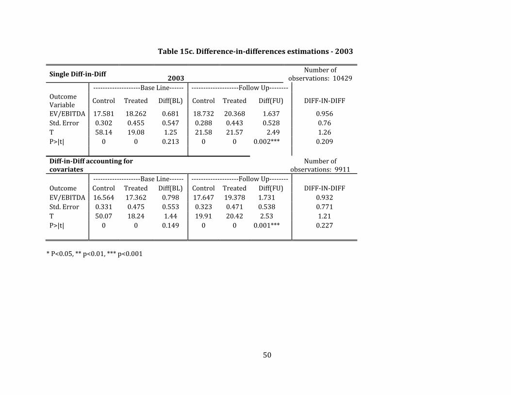
50
Table15c.Difference‐in‐differencesestimations‐2003
SingleDiff‐in‐Diff 2003 Numberof
observations:10429 ‐‐‐‐‐‐‐‐‐‐‐‐‐‐‐‐‐‐‐‐BaseLine‐‐‐‐‐‐ ‐‐‐‐‐‐‐‐‐‐‐‐‐‐‐‐‐‐‐‐FollowUp‐‐‐‐‐‐‐‐OutcomeVariable
Control Treated Diff(BL) Control Treated Diff(FU) DIFF‐IN‐DIFF
EV/EBITDA 17.581 18.262 0.681 18.732 20.368 1.637 0.956Std.Error 0.302 0.455 0.547 0.288 0.443 0.528 0.76T 58.14 19.08 1.25 21.58 21.57 2.49 1.26P>|t| 0 0 0.213 0 0 0.002*** 0.209 Diff‐in‐Diffaccountingforcovariates Numberof
observations:9911 ‐‐‐‐‐‐‐‐‐‐‐‐‐‐‐‐‐‐‐‐BaseLine‐‐‐‐‐‐ ‐‐‐‐‐‐‐‐‐‐‐‐‐‐‐‐‐‐‐‐FollowUp‐‐‐‐‐‐‐‐ Outcome Control Treated Diff(BL) Control Treated Diff(FU) DIFF‐IN‐DIFFEV/EBITDA 16.564 17.362 0.798 17.647 19.378 1.731 0.932Std.Error 0.331 0.475 0.553 0.323 0.471 0.538 0.771T 50.07 18.24 1.44 19.91 20.42 2.53 1.21P>|t| 0 0 0.149 0 0 0.001*** 0.227 *P<0.05,**p<0.01,***p<0.001
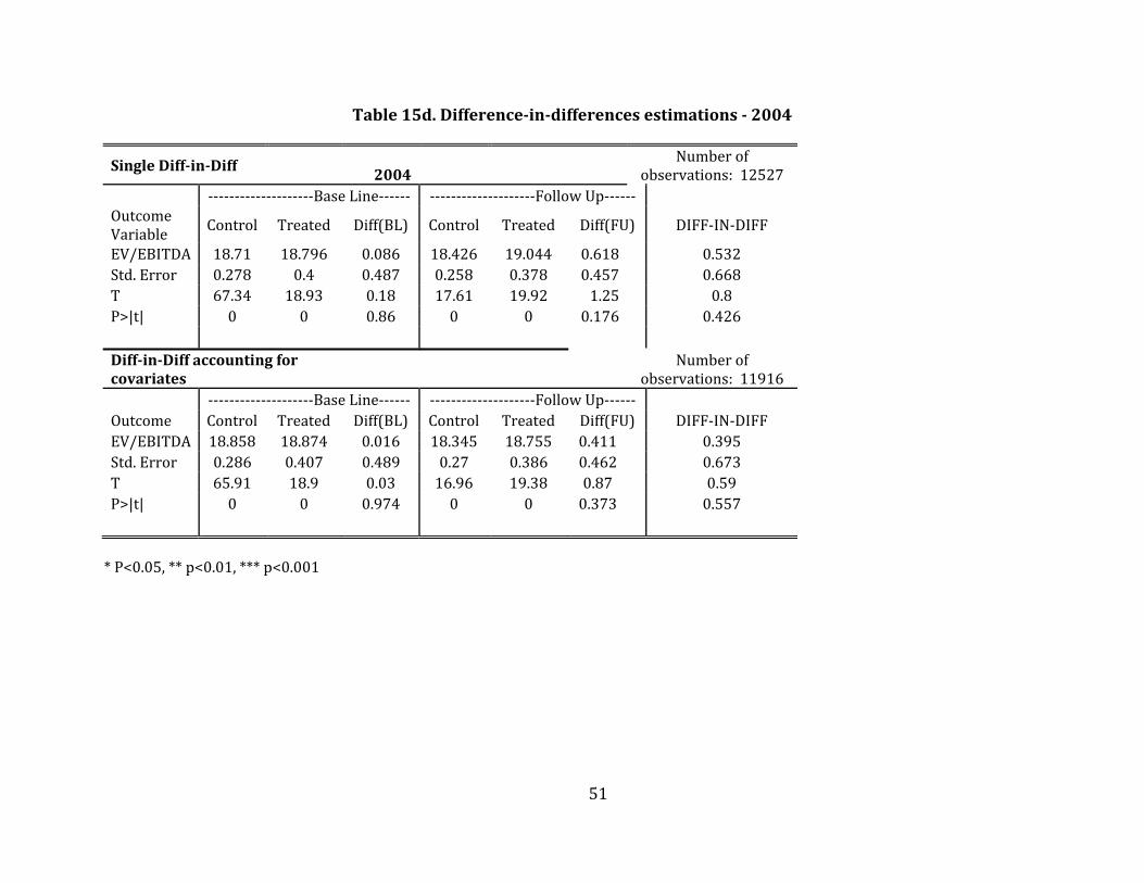
51
Table15d.Difference‐in‐differencesestimations‐2004
SingleDiff‐in‐Diff 2004 Numberof
observations:12527 ‐‐‐‐‐‐‐‐‐‐‐‐‐‐‐‐‐‐‐‐BaseLine‐‐‐‐‐‐ ‐‐‐‐‐‐‐‐‐‐‐‐‐‐‐‐‐‐‐‐FollowUp‐‐‐‐‐‐OutcomeVariable
Control Treated Diff(BL) Control Treated Diff(FU) DIFF‐IN‐DIFF
EV/EBITDA 18.71 18.796 0.086 18.426 19.044 0.618 0.532Std.Error 0.278 0.4 0.487 0.258 0.378 0.457 0.668T 67.34 18.93 0.18 17.61 19.92 1.25 0.8P>|t| 0 0 0.86 0 0 0.176 0.426 Diff‐in‐Diffaccountingforcovariates Numberof
observations:11916 ‐‐‐‐‐‐‐‐‐‐‐‐‐‐‐‐‐‐‐‐BaseLine‐‐‐‐‐‐ ‐‐‐‐‐‐‐‐‐‐‐‐‐‐‐‐‐‐‐‐FollowUp‐‐‐‐‐‐ Outcome Control Treated Diff(BL) Control Treated Diff(FU) DIFF‐IN‐DIFFEV/EBITDA 18.858 18.874 0.016 18.345 18.755 0.411 0.395Std.Error 0.286 0.407 0.489 0.27 0.386 0.462 0.673T 65.91 18.9 0.03 16.96 19.38 0.87 0.59P>|t| 0 0 0.974 0 0 0.373 0.557 *P<0.05,**p<0.01,***p<0.001
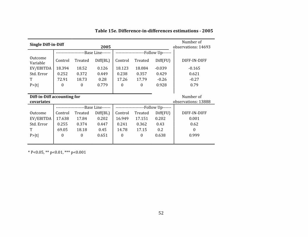
52
Table15e.Difference‐in‐differencesestimations‐2005
SingleDiff‐in‐Diff 2005 Numberof
observations:14693 ‐‐‐‐‐‐‐‐‐‐‐‐‐‐‐‐‐‐‐‐BaseLine‐‐‐‐‐‐ ‐‐‐‐‐‐‐‐‐‐‐‐‐‐‐‐‐‐‐‐FollowUp‐‐‐‐‐‐OutcomeVariable
Control Treated Diff(BL) Control Treated Diff(FU) DIFF‐IN‐DIFF
EV/EBITDA 18.394 18.52 0.126 18.123 18.084 ‐0.039 ‐0.165Std.Error 0.252 0.372 0.449 0.238 0.357 0.429 0.621T 72.91 18.73 0.28 17.26 17.79 ‐0.26 ‐0.27P>|t| 0 0 0.779 0 0 0.928 0.79 Diff‐in‐Diffaccountingforcovariates Numberof
observations:13888 ‐‐‐‐‐‐‐‐‐‐‐‐‐‐‐‐‐‐‐‐BaseLine‐‐‐‐‐‐ ‐‐‐‐‐‐‐‐‐‐‐‐‐‐‐‐‐‐‐‐FollowUp‐‐‐‐‐‐ Outcome Control Treated Diff(BL) Control Treated Diff(FU) DIFF‐IN‐DIFFEV/EBITDA 17.638 17.84 0.202 16.949 17.151 0.202 0.001Std.Error 0.255 0.374 0.447 0.241 0.362 0.43 0.62T 69.05 18.18 0.45 14.78 17.15 0.2 0P>|t| 0 0 0.651 0 0 0.638 0.999 *P<0.05,**p<0.01,***p<0.001

53
Table15f.Difference‐in‐differencesestimations‐2006
SingleDiff‐in‐Diff 2006 Numberof
observations:16097 ‐‐‐‐‐‐‐‐‐‐‐‐‐‐‐‐‐‐‐‐BaseLine‐‐‐‐‐‐ ‐‐‐‐‐‐‐‐‐‐‐‐‐‐‐‐‐‐‐‐FollowUp‐‐‐‐‐‐OutcomeVariable
Control Treated Diff(BL) Control Treated Diff(FU) DIFF‐IN‐DIFF
EV/EBITDA 17.381 18.557 1.176 18.884 19.472 0.588 ‐0.588Std.Error 0.247 0.339 0.419 0.233 0.327 0.401 0.58T 70.49 20.85 2.8 23.85 18.26 ‐0.29 ‐1.01P>|t| 0 0 0.005*** 0 0 0.143 0.311 Diff‐in‐Diffaccountingforcovariates Numberof
observations:15247 ‐‐‐‐‐‐‐‐‐‐‐‐‐‐‐‐‐‐‐‐BaseLine‐‐‐‐‐‐ ‐‐‐‐‐‐‐‐‐‐‐‐‐‐‐‐‐‐‐‐FollowUp‐‐‐‐‐‐ Outcome Control Treated Diff(BL) Control Treated Diff(FU) DIFF‐IN‐DIFFEV/EBITDA 16.686 17.811 1.124 18.442 18.911 0.469 ‐0.655Std.Error 0.249 0.342 0.419 0.237 0.332 0.403 0.581T 66.96 19.97 2.68 24.11 17.59 ‐0.5 ‐1.13P>|t| 0 0 0.007*** 0 0 0.245 0.259 *P<0.05,**p<0.01,***p<0.001
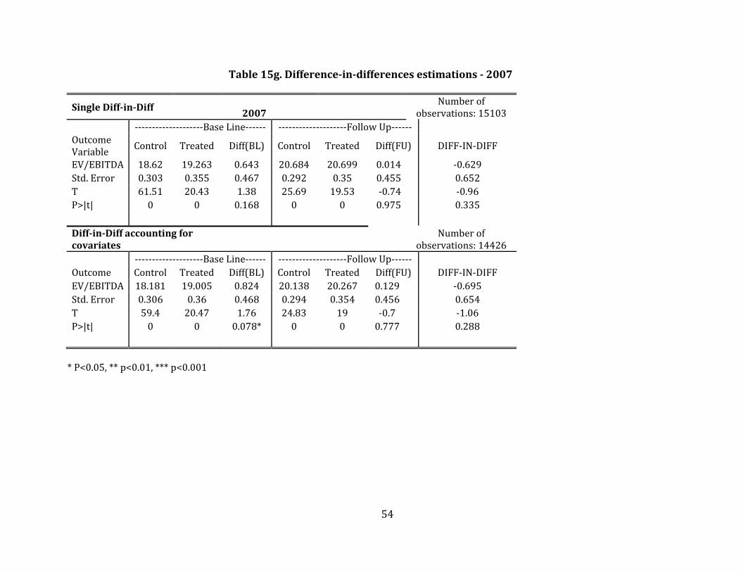
54
Table15g.Difference‐in‐differencesestimations‐2007
SingleDiff‐in‐Diff 2007 Numberof
observations:15103 ‐‐‐‐‐‐‐‐‐‐‐‐‐‐‐‐‐‐‐‐BaseLine‐‐‐‐‐‐ ‐‐‐‐‐‐‐‐‐‐‐‐‐‐‐‐‐‐‐‐FollowUp‐‐‐‐‐‐OutcomeVariable
Control Treated Diff(BL) Control Treated Diff(FU) DIFF‐IN‐DIFF
EV/EBITDA 18.62 19.263 0.643 20.684 20.699 0.014 ‐0.629Std.Error 0.303 0.355 0.467 0.292 0.35 0.455 0.652T 61.51 20.43 1.38 25.69 19.53 ‐0.74 ‐0.96P>|t| 0 0 0.168 0 0 0.975 0.335 Diff‐in‐Diffaccountingforcovariates Numberof
observations:14426 ‐‐‐‐‐‐‐‐‐‐‐‐‐‐‐‐‐‐‐‐BaseLine‐‐‐‐‐‐ ‐‐‐‐‐‐‐‐‐‐‐‐‐‐‐‐‐‐‐‐FollowUp‐‐‐‐‐‐ Outcome Control Treated Diff(BL) Control Treated Diff(FU) DIFF‐IN‐DIFFEV/EBITDA 18.181 19.005 0.824 20.138 20.267 0.129 ‐0.695Std.Error 0.306 0.36 0.468 0.294 0.354 0.456 0.654T 59.4 20.47 1.76 24.83 19 ‐0.7 ‐1.06P>|t| 0 0 0.078* 0 0 0.777 0.288 *P<0.05,**p<0.01,***p<0.001
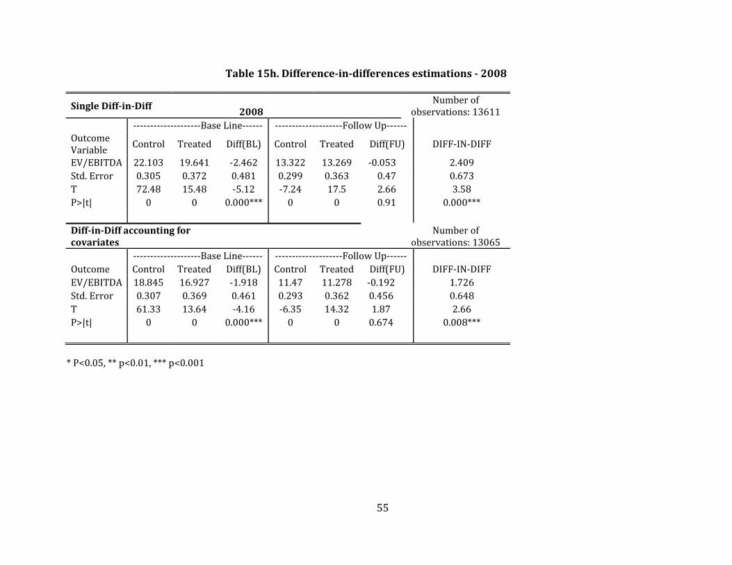
55
Table15h.Difference‐in‐differencesestimations‐2008
SingleDiff‐in‐Diff 2008 Numberof
observations:13611 ‐‐‐‐‐‐‐‐‐‐‐‐‐‐‐‐‐‐‐‐BaseLine‐‐‐‐‐‐ ‐‐‐‐‐‐‐‐‐‐‐‐‐‐‐‐‐‐‐‐FollowUp‐‐‐‐‐‐OutcomeVariable
Control Treated Diff(BL) Control Treated Diff(FU) DIFF‐IN‐DIFF
EV/EBITDA 22.103 19.641 ‐2.462 13.322 13.269 ‐0.053 2.409Std.Error 0.305 0.372 0.481 0.299 0.363 0.47 0.673T 72.48 15.48 ‐5.12 ‐7.24 17.5 2.66 3.58P>|t| 0 0 0.000*** 0 0 0.91 0.000*** Diff‐in‐Diffaccountingforcovariates Numberof
observations:13065 ‐‐‐‐‐‐‐‐‐‐‐‐‐‐‐‐‐‐‐‐BaseLine‐‐‐‐‐‐ ‐‐‐‐‐‐‐‐‐‐‐‐‐‐‐‐‐‐‐‐FollowUp‐‐‐‐‐‐ Outcome Control Treated Diff(BL) Control Treated Diff(FU) DIFF‐IN‐DIFFEV/EBITDA 18.845 16.927 ‐1.918 11.47 11.278 ‐0.192 1.726Std.Error 0.307 0.369 0.461 0.293 0.362 0.456 0.648T 61.33 13.64 ‐4.16 ‐6.35 14.32 1.87 2.66P>|t| 0 0 0.000*** 0 0 0.674 0.008*** *P<0.05,**p<0.01,***p<0.001

56
Table15i.Difference‐in‐differencesestimations‐2009
SingleDiff‐in‐Diff 2009 Numberof
observations:8416 ‐‐‐‐‐‐‐‐‐‐‐‐‐‐‐‐‐‐‐‐BaseLine‐‐‐‐‐‐ ‐‐‐‐‐‐‐‐‐‐‐‐‐‐‐‐‐‐‐‐FollowUp‐‐‐‐‐‐‐OutcomeVariable
Control Treated Diff(BL) Control Treated Diff(FU) DIFF‐IN‐DIFF
EV/EBITDA 12.97 13.718 0.748 16.682 17.737 1.056 0.308Std.Error 0.365 0.387 0.532 0.354 0.386 0.524 0.747T 35.55 14.9 1.41 23.45 18.23 1.34 0.41P>|t| 0 0 0.16 0 0 0.044** 0.68 Diff‐in‐Diffaccountingforcovariates Numberof
observations:8145 ‐‐‐‐‐‐‐‐‐‐‐‐‐‐‐‐‐‐‐‐BaseLine‐‐‐‐‐ ‐‐‐‐‐‐‐‐‐‐‐‐‐‐‐‐‐‐‐‐FollowUp‐‐‐‐‐‐‐ Outcome Control Treated Diff(BL) Control Treated Diff(FU) DIFF‐IN‐DIFFEV/EBITDA 11.536 12.151 0.615 14.76 15.981 1.221 0.606Std.Error 0.384 0.405 0.522 0.382 0.409 0.515 0.733T 30.02 13.05 1.18 19.98 16.86 1.79 0.83P>|t| 0 0 0.239 0 0 0.018** 0.408 *P<0.05,**p<0.01,***p<0.001

57
Figure3.Trendofenterprisemultiplebysector
15
18
21
‐3 ‐2 ‐1 0 1 2 3
EV/EBITD
A
dt
Communication Energy Technology Utilities
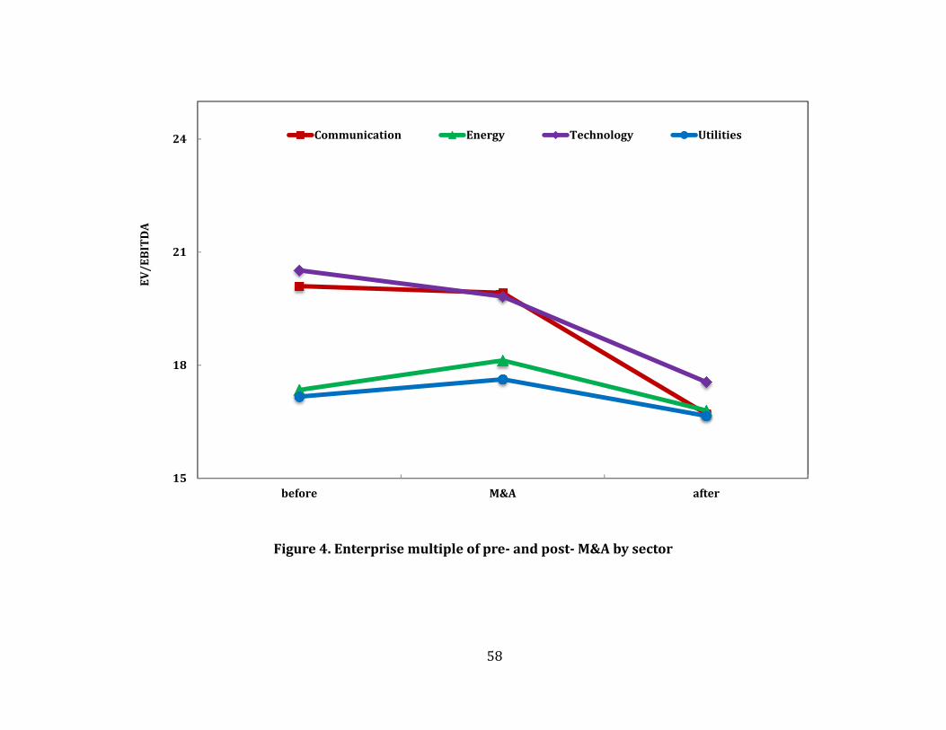
58
Figure4.Enterprisemultipleofpre‐andpost‐M&Abysector
15
18
21
24
before M&A after
EV/EBITD
ACommunication Energy Technology Utilities

59